Automatic Generation of Probabilistic Programming from Time Series Data

Anh Tong and Jaesik ChoiUlsan National Institute of Science and Technology

Ulsan, 44919 Korea{anhth,jaesik}@unist.ac.kr

AbstractProbabilistic programming languages represent com-plex data with intermingled models in a few lines ofcode. Efficient inference algorithms in probabilisticprogramming languages make possible to build unifiedframeworks to compute interesting probabilities of var-ious large, real-world problems. When the structure ofmodel is given, constructing a probabilistic program israther straightforward. Thus, main focus have been tolearn the best model parameters and compute marginalprobabilities. In this paper, we provide a new perspec-tive to build expressive probabilistic program from con-tinue time series data when the structure of model isnot given. The intuition behind of our method is tofind a descriptive covariance structure of time seriesdata in nonparametric Gaussian process regression. Wereport that such descriptive covariance structure effi-ciently derives a probabilistic programming descriptionaccurately.

IntroductionProbabilistic programming has potential impacts on vari-ous works in artificial intelligence, machine learning, statis-tics, robotics (Lebeltel et al. (2004)), vision (Kulkarni etal. (2015)), neuroscience (Lake, Salakhutdinov, and Tenen-baum (2015)), and cognitive science (Freer, Roy, and Tenen-baum (2012)). Many different approaches and probabilis-tic programming languages are introduced, for example,Church (Goodman et al., 2012), Problog (De Raedt, Kim-mig, and Toivonen, 2007), BUGS (Lunn et al., 2000), Stan(Carpenter, 2015). Although each probabilistic program-ming language has its own strength and domain, we chooseStan to present our work in this paper since it is suitablefor modeling continuous signal.

The Automatic Bayesian Covariance Discovery (ABCD)system which is so-called automatic statistician system, isproposed (Lloyd et al., 2014) with the aim of automat-ing the process of statistical modeling. It focuses on re-gression problems. Specifically, it takes time series as in-put, searches and then produces a learned Gaussian processmodel which has interpretable properties (smoothness, pe-riodicity, changepoints) and is summarized with a report.With the same purpose, (Hwang, Tong, and Choi, 2016) pro-posed a relational approach to handle multiple data. How-ever, such kinds of modeling usually require a body of work

and efforts to make build a new model. One of the advan-tages of probabilistic programming which helps in this situ-ation is the ease of creating generative models with severallines of code (Kulkarni et al., 2015). In order to facilitate theprocess of building new ABCD-based models, we proposea method generating Stan probabilistic programming fromABCD results. Time series are stored in the compact rep-resentation of encoded ABCD probabilistic programmingswhich potentially allow construct a complex model fromheterogeneous models.

This paper is organized as follows. We briefly introducethe background of Gaussian Processes (GP) , the ABCD sys-tem and its relational version for multiple data. Then, wepresent our main contribution on how a probabilistic pro-gramming is generated from time series data; Next is theexperiment section; Finally, we conclude our work.

BackgroundAutomatic Statistician SystemAutomatic Bayesian Covariance Discovery (ABCD) ex-plains data without requiring expert input for regressionproblems. Here the approach is to use Gaussian processesto model regression functions.

Let us take a brief overview about Gaussian Pro-cesses (GPs). GPs are distributions over functions suchthat any finite set of function evaluations, f(x) =(f(x1), f(x2), . . . , f(xN )) form a multivariate Gaussiandistribution (Rasmussen and Williams, 2006). It is specifiedby a mean function µ(x) = E[f(x)] and a covariance kernelfunction k(x, x′) = Cov(f(x), f(x’)). Evaluations of the twofunctions on a finite set of points correspond to the meanvector and the covariance matrix for the multivariate Gaus-sian distribution, like µi=µ(xi) and Σij=k(xi, xj). Whena function or evaluations of the function f are drawn from aGaussian Process (GP) specified by its mean function µ(x)and covariance kernel function k(x, x′),

f ∼ GP(µ(x), k(x, x′))

Covariance kernel function plays a crucial role in a GP, asit conveys our assumptions about the function. Duvenaud etal. (2013) proposed a compositional kernel learning method.It constructs and find richer kernel which are composed ofserver base kernels and operation. In theory, any positivedefinite kernels are closed under addition and multiplication.

arX

iv:1

607.

0071

0v2

[st

at.M

L]

14

Jul 2

016

Five base kernels are used for making composi-tional kernels. Each kernel encodes different charac-teristics of functions, which further enables the gen-eralization of structure and inference given new data.

Base Kernels Encoding FunctionWhite Noise (WN) Uncorrelated noise

Constant (C) Constant functionsLinear (LIN) Linear functions

Squared Exponential (SE) Smooth functionsPeriodic (PER) Periodic functions

The first operation is addition which sums multiple kernelfunctions and makes a new kernel function.

k′(x, x′) = k1(x, x′) + k2(x, x′).

ABCD assumes zero mean for GPs, since marginalizingover an unknown mean function can be equivalently ex-pressed as a zero-mean GP with a new kernel (Lloyd et al.,2014). Under this assumption, the following multiplicationoperation is also applicable.

k′(x, x′) = k1(x, x′)× k2(x, x′).

The third operation is the change-point (CP) operation.Given two kernel functions, k1 and k2, the new kernel func-tion is represented as follows:

k′(x, x′) = σ(x)k1(x, x′)σ(x′)

+ (1− σ(x))k2(x, x′)(1− σ(x′))

where σ(x) is a sigmoidal function which lies between 0 and1, and ` is the change-point. The change-point operation di-vides function domain (i.e., time) into two sides and appliesdifferent kernel function on each side.

Finally, the change-window (CW) operation applies theCP operation twice with two different change points `1 and`2. Given two sigmoidal functions σ1(x; `1) and σ2(x; `2)where `1 < `2, the new function will be f := σ1(x)f1(1 −σ2(x))+(1−σ1(x))f2σ2(x), which applies the function f1to the window (`1, `2). A composite kernel expression afterthe change-window operation will be as follows:

k′(x, x′) = σ1(x)(1− σ2(x))k1(x, x′)σ1(x′)(1− σ2(x′))

+ (1− σ1(x))σ2(x)k2(x, x′)(1− σ1(x′))σ2(x′).

ABCD searches a composite kernel based on the searchgrammar. The search grammar specifies how to develop thecurrent kernel expression by applying the operations withthe base kernels. The following rules are examples of typicalsearch grammar:

S → S + B S → S × BS → CP(S,S) S → CW(S,S)

S → B S → C

where S represents any kernel subexpression, B and B′ arebase kernels.

Given data and a maximum search depth, the algorithmgives a compositional kernel k(x, x′; θ). Starting from theWN kernel, the algorithm expands the kernel expressionbased on the search grammar, optimizes hyperparameters forthe expanded kernels, evaluates those kernels given the data

yififGPσj

kdj (x, x′)

kS(x, x′)µ(x)

0 kS θ

G

i ∈ 1...N

j ∈ 1...M

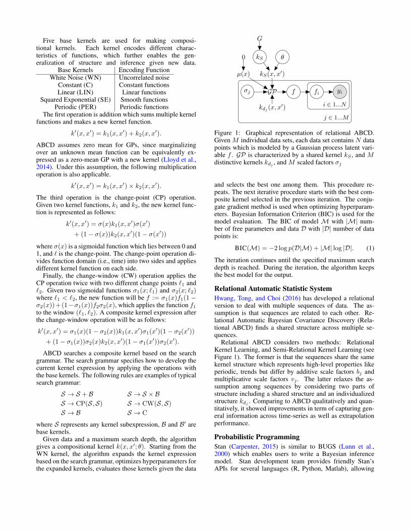
Figure 1: Graphical representation of relational ABCD.Given M individual data sets, each data set contains N datapoints which is modeled by a Gaussian process latent vari-able f . GP is characterized by a shared kernel kS , and Mdistinctive kernels kdj , and M scaled factors σj

and selects the best one among them. This procedure re-peats. The next iterative procedure starts with the best com-posite kernel selected in the previous iteration. The conju-gate gradient method is used when optimizing hyperparam-eters. Bayesian Information Criterion (BIC) is used for themodel evaluation. The BIC of model M with |M| num-ber of free parameters and data D with |D| number of datapoints is:

BIC(M) = −2 log p(D|M) + |M| log |D|. (1)

The iteration continues until the specified maximum searchdepth is reached. During the iteration, the algorithm keepsthe best model for the output.

Relational Automatic Statistic SystemHwang, Tong, and Choi (2016) has developed a relationalversion to deal with multiple sequences of data. The as-sumption is that sequences are related to each other. Re-lational Automatic Bayesian Covariance Discovery (Rela-tional ABCD) finds a shared structure across multiple se-quences.

Relational ABCD considers two methods: RelationalKernel Learning, and Semi-Relational Kernel Learning (seeFigure 1). The former is that the sequences share the samekernel structure which represents high-level properties likeperiodic, trends but differ by additive scale factors bj andmultiplicative scale factors vj . The latter relaxes the as-sumption among sequences by considering two parts ofstructure including a shared structure and an individualizedstructure kdj . Comparing to ABCD qualitatively and quan-titatively, it showed improvements in term of capturing gen-eral information across time-series as well as extrapolationperformance.

Probabilistic ProgrammingStan (Carpenter, 2015) is similar to BUGS (Lunn et al.,2000) which enables users to write a Bayesian inferencemodel. Stan development team provides friendly Stan’sAPIs for several languages (R, Python, Matlab), allowing

access to many type of users. The fundamental concept usedin Stan is the No U-Turn (NUTS) sampler (Homan and Gel-man, 2014) which builds a tree of possible samples by ran-domly simulating Hamiltonian dynamics both forwards andbackwards in time until the combined trajectory turns backon itself.

data {// N >= 0int<lower=0> N;// y[n] in { 0, 1 }int<lower=0,upper=1> y[N];

}parameters {

// theta in [0, 1]real<lower=0,upper=1> theta;

}model {

// priortheta ˜ beta(1,1);// likelihoodfor (n in 1:N)

y[n] ˜ bernoulli(theta);}

Figure 2: A sample Stan code for estimating a Bernoulliparameter

A sample Stan code is showed in Figure 2 which con-siders estimating the chance of success parameter for aBernoulli distribution based on a sequence of observer bi-nary outcomes. Here the assumption is that N binarydata y[1],..., y[N] is independent and identically dis-tributed, with success probability theta. The model makesthe prior assumption beta(1,1) on theta. Then, thedata is fitted in the loop for (n in 1:N)

The followings are concentrated on how a Stan programis structured and executed.

• Data block Data block declares the data to fit the model.In the Figure 2, the data block declares an integer valueN which is the number of observed data. The array y hassize N, containing information of success outcomes. It isable to set constraints of data with an upper bound upperand a lower bound lower.

• Transformed data block A transformed data block is usedto define a new auxiliary variables which is computedfrom data, containing mediate information. Figure 2 doesnot include the transformed data block.Parameter block In Figure 2, the program has only one pa-rameter theta defined in the parameter block. We alsocan set constraints on parameters.

• Transformed parameter block The transformed parameterblock defines transforms of parameters for a model. It isoptional, and does not appear in Figure 2.

• Model block The model block defines the log probabilityfunction on the parameter space. In the program, by pro-viding the prior on theta, the likelihood is evaluated.

• Generated quantities block The (optional) generatedquantities allows values that depend on parameters anddata. It may be used to calculate predictive inferences. Itcan carry out forward simulation for predictive posteriorchecks.

Automatic Generation of ProbabilisticProgramming

Generating probabilistic programming from ABCD and/orrelational ABCD is a crucial component in the system weaim to build (see Figure 3). Prior to this component, one canchoose either ABCD or relational ABCD based on whetherthe preference is for a single time series or for global infor-mation in multiple time series. Both ABCD and relationalABCD play as producers which output compositional ker-nels from data (Step 1 and 2). Step 4 and 5 are an exampleapplication. We will discuss what is inside Step 3 in thissection.

From now on, we use the notation StanABCD to indi-cate the Stan probabilistic programs generated automati-cally from ABCD.

Base kernelsAn ABCD’s result is represented by a compositional struc-ture which is a sum of products of base kernels. This sum-mation is the outcome of simplifications: the multiplicationof two SE kernel produces another SE with different param-eter values. The product of WN and any stationary ker-nel including C, PER, WN, SE results a new WN kernel.Multiplying C with any kernel does not change the kernelbut changes the scale parameter of that kernel (Lloyd et al.,2014). Hence, let G be a set of all possible kernel expres-sions, written as

G = {∑

k∏m

LIN(m)σ(n)}

where σ is the sigmoid function, k is in

K = {WN,C,∏k

PER(k),SE∏k

PER(k)}

For example, a learned compositional kernel is describedas

SE× LIN (2)

Here, the square exponential kernel and linear kernel arewritten respectively as

SE(x, x′) = σ2 exp

(− (x− x′)2

2l2

),

LIN(x, x′) = σ2(x− l)(x′ − l).The kernel (2) can be understood linguistically as ’a smoothfunction with linearly (LIN) increasing amplitude’.

Another real-world example is a chosen currency ex-change data set (see Figure 5). The data set containsexchange value of Indonesian Rupiad from 2015-06-28to 2015-12-30 acquired from Yahoo Finance (Yahoo Inc.,

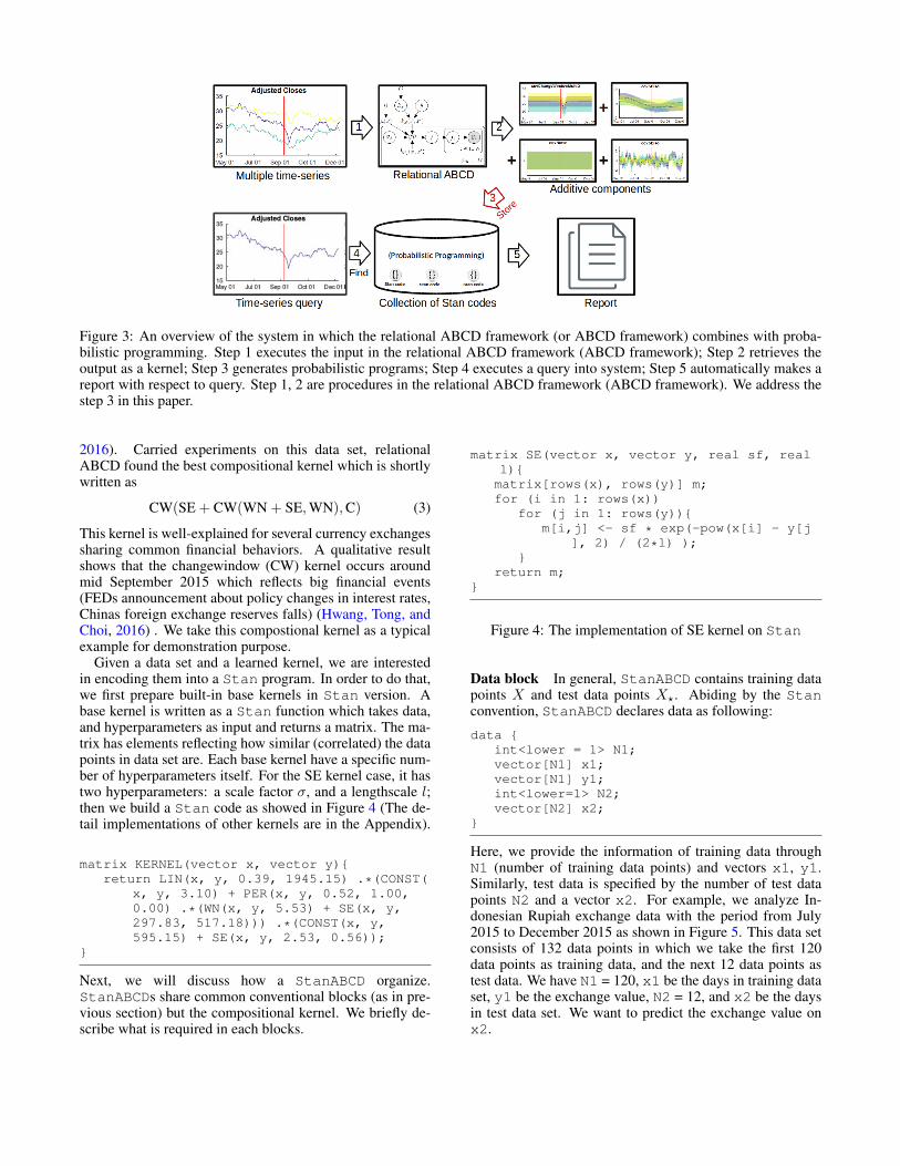
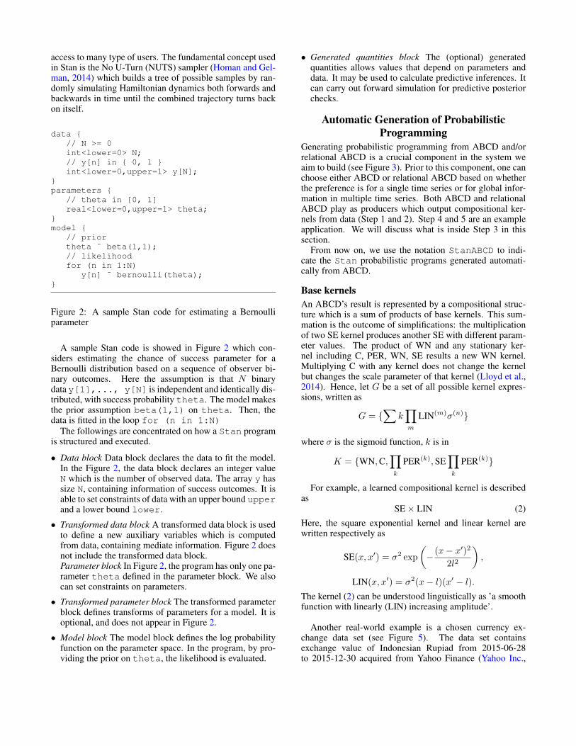
Figure 3: An overview of the system in which the relational ABCD framework (or ABCD framework) combines with proba-bilistic programming. Step 1 executes the input in the relational ABCD framework (ABCD framework); Step 2 retrieves theoutput as a kernel; Step 3 generates probabilistic programs; Step 4 executes a query into system; Step 5 automatically makes areport with respect to query. Step 1, 2 are procedures in the relational ABCD framework (ABCD framework). We address thestep 3 in this paper.

2016). Carried experiments on this data set, relationalABCD found the best compositional kernel which is shortlywritten as

CW(SE + CW(WN + SE,WN),C) (3)

This kernel is well-explained for several currency exchangessharing common financial behaviors. A qualitative resultshows that the changewindow (CW) kernel occurs aroundmid September 2015 which reflects big financial events(FEDs announcement about policy changes in interest rates,Chinas foreign exchange reserves falls) (Hwang, Tong, andChoi, 2016) . We take this compostional kernel as a typicalexample for demonstration purpose.

Given a data set and a learned kernel, we are interestedin encoding them into a Stan program. In order to do that,we first prepare built-in base kernels in Stan version. Abase kernel is written as a Stan function which takes data,and hyperparameters as input and returns a matrix. The ma-trix has elements reflecting how similar (correlated) the datapoints in data set are. Each base kernel have a specific num-ber of hyperparameters itself. For the SE kernel case, it hastwo hyperparameters: a scale factor σ, and a lengthscale l;then we build a Stan code as showed in Figure 4 (The de-tail implementations of other kernels are in the Appendix).

matrix KERNEL(vector x, vector y){return LIN(x, y, 0.39, 1945.15) .*(CONST(

x, y, 3.10) + PER(x, y, 0.52, 1.00,0.00) .*(WN(x, y, 5.53) + SE(x, y,297.83, 517.18))) .*(CONST(x, y,595.15) + SE(x, y, 2.53, 0.56));

}

Next, we will discuss how a StanABCD organize.StanABCDs share common conventional blocks (as in pre-vious section) but the compositional kernel. We briefly de-scribe what is required in each blocks.

matrix SE(vector x, vector y, real sf, reall){matrix[rows(x), rows(y)] m;for (i in 1: rows(x))

for (j in 1: rows(y)){m[i,j] <- sf * exp(-pow(x[i] - y[j

], 2) / (2*l) );}

return m;}

Figure 4: The implementation of SE kernel on Stan

Data block In general, StanABCD contains training datapoints X and test data points X?. Abiding by the Stanconvention, StanABCD declares data as following:

data {int<lower = 1> N1;vector[N1] x1;vector[N1] y1;int<lower=1> N2;vector[N2] x2;

}

Here, we provide the information of training data throughN1 (number of training data points) and vectors x1, y1.Similarly, test data is specified by the number of test datapoints N2 and a vector x2. For example, we analyze In-donesian Rupiah exchange data with the period from July2015 to December 2015 as shown in Figure 5. This data setconsists of 132 data points in which we take the first 120data points as training data, and the next 12 data points astest data. We have N1 = 120, x1 be the days in training dataset, y1 be the exchange value, N2 = 12, and x2 be the daysin test data set. We want to predict the exchange value onx2.

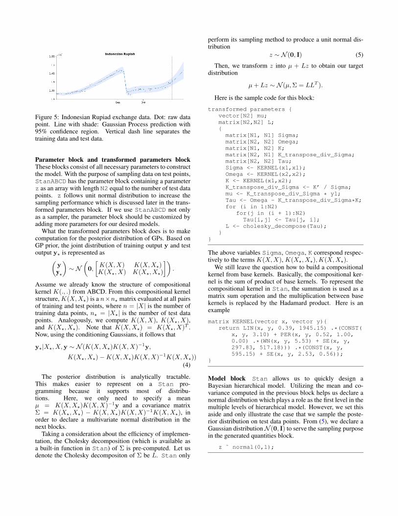
Figure 5: Indonesian Rupiad exchange data. Dot: raw datapoint. Line with shade: Gaussian Process prediction with95% confidence region. Vertical dash line separates thetraining data and test data.

Parameter block and transformed parameters blockThese blocks consist of all necessary parameters to constructthe model. With the purpose of sampling data on test points,StanABCD has the parameter block containing a parameterz as an array with length N2 equal to the number of test datapoints. z follows unit normal distribution to increase thesampling performance which is discussed later in the trans-formed parameters block. If we use StanABCD not onlyas a sampler, the parameter block should be customized byadding more parameters for our desired models.

What the transformed parameters block does is to makecomputation for the posterior distribution of GPs. Based onGP prior, the joint distribution of training output y and testoutput y? is represented as(

yy?

)∼ N

(0,

[K(X,X) K(X,X?)K(X?, X) K(X?, X?)

]).

Assume we already know the structure of compositionalkernel K(., .) from ABCD. From this compositional kernelstructure, K(X,X?) is a n×n? matrix evaluated at all pairsof training and test points, where n = |X| is the number oftraining data points, n? = |X?| is the number of test datapoints. Analogously, we compute K(X,X), K(X?, X),and K(X?, X?). Note that K(X,X?) = K(X?, X)T .Now, using the conditioning Gaussians, it follows that

y?|X?, X,y ∼ N (K(X,X?)K(X,X)−1y,

K(X?, X?)−K(X,X?)K(X,X)−1K(X,X?))(4)

The posterior distribution is analytically tractable.This makes easier to represent on a Stan pro-gramming because it supports most of distribu-tions. Here, we only need to specify a meanµ = K(X,X?)K(X,X)−1y and a covariance matrixΣ = K(X?, X?) − K(X,X?)K(X,X)−1K(X,X?), inorder to declare a multivariate normal distribution in thenext blocks.

Taking a consideration about the efficiency of implemen-tation, the Cholesky decomposition (which is available asa built-in function in Stan) of Σ is pre-computed. Let usdenote the Cholesky decompositon of Σ be L. Stan only

perform its sampling method to produce a unit normal dis-tribution

z ∼ N (0, I) (5)

Then, we transform z into µ + Lz to obtain our targetdistribution

µ+ Lz ∼ N (µ,Σ = LLT ).

Here is the sample code for this block:

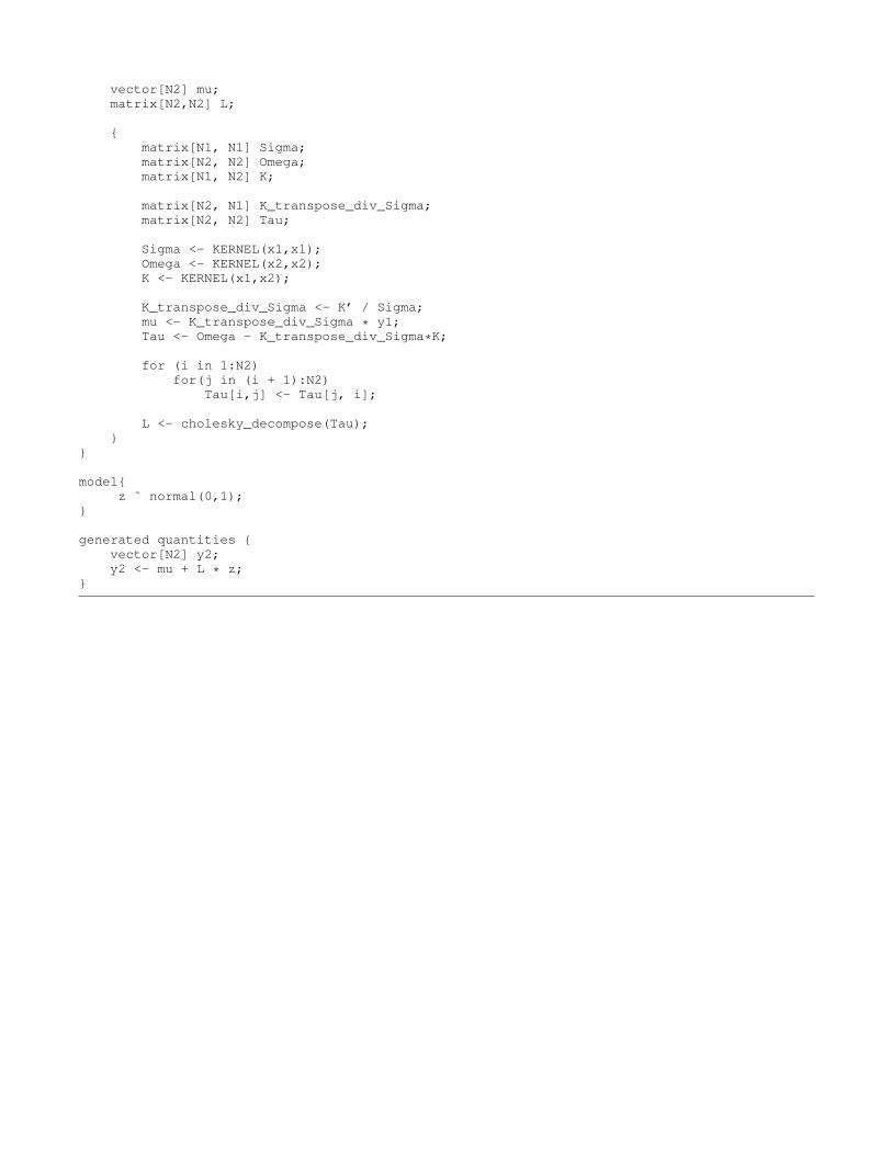
transformed parameters {vector[N2] mu;matrix[N2,N2] L;{

matrix[N1, N1] Sigma;matrix[N2, N2] Omega;matrix[N1, N2] K;matrix[N2, N1] K_transpose_div_Sigma;matrix[N2, N2] Tau;Sigma <- KERNEL(x1,x1);Omega <- KERNEL(x2,x2);K <- KERNEL(x1,x2);K_transpose_div_Sigma <- K’ / Sigma;mu <- K_transpose_div_Sigma * y1;Tau <- Omega - K_transpose_div_Sigma*K;for (i in 1:N2)

for(j in (i + 1):N2)Tau[i,j] <- Tau[j, i];

L <- cholesky_decompose(Tau);}

}

The above variables Sigma, Omega, K correspond respec-tively to the terms K(X,X), K(X?, X?),K(X,X?).

We still leave the question how to build a compositionalkernel from base kernels. Basically, the compositional ker-nel is the sum of product of base kernels. To represent thecompositional kernel in Stan, the summation is used as amatrix sum operation and the multiplication between basekernels is replaced by the Hadamard product. Here is anexample

matrix KERNEL(vector x, vector y){return LIN(x, y, 0.39, 1945.15) .*(CONST(

x, y, 3.10) + PER(x, y, 0.52, 1.00,0.00) .*(WN(x, y, 5.53) + SE(x, y,297.83, 517.18))) .*(CONST(x, y,595.15) + SE(x, y, 2.53, 0.56));

}

Model block Stan allows us to quickly design aBayesian hierarchical model. Utilizing the mean and co-variance computed in the previous block helps us declare anormal distribution which plays a role as the first level in themultiple levels of hierarchical model. However, we set thisaside and only illustrate the case that we sample the poste-rior distribution on test data points. From (5), we declare aGaussian distributionN (0, I) to serve the sampling purposein the generated quantities block.

z ˜ normal(0,1);

(a)

(b)

Figure 6: A comparison of ABCD result and StanABCD’ssample extrapolation (from dash line). a) Extraplation ofairline data from ABCD (Lloyd et al., 2014). b) Generatedsample from StanABCD

Generated quantities block For purpose of generatingsample extrapolation value, the normal distribution declaredin the model block will be called one time.

generated quantities {vector[N2] y2;y2 <- mu + L * z;

}

In order to get the sample of test output y2, the above Stancode performs the linear transformation on sample valuesgenerated from z (N (0, I)) as we explained in the trans-formed parameters block.

ExperimentData set Beside the Indonesian Rupiah exchange datamentioned in previous section, we select a airline data setto perform experiments on. The data set describes monthlyinternational airline passenger numbers for the period be-tween January 1949 and December 1960 (George E. P. Box(2013)). The number of passengers was periodic with a typ-ical period 1 year. The total number of passengers per yearincreased monotonically. ABCD captures this informationwell, and explain the data set by a compositional kernel: LIN+ SE × PER × LIN + SE + WN × LIN.

Sampling data We provide a complete sample Stan codein the appendix. We want to get extrapolation sample valueson test points (from January 1961) of airline data set. Dur-ing the experiment, we use Python to retrieve data set thenpass to Stan compiler through PyStan (Stan DevelopmentTeam, 2016). Figure 6 and 7 show that StanABCD pro-vides similar results as ABCD in the view of extrapolationperformance. Our generating method guarantees a reliableway to perform one-to-one mapping from ABCD result intoa probabilistic programming.

Figure 7: The extrapolation sampling (from vertical dashline) from StanABCD for Indonesian Rupiah data set.Comparing to ABCD result (see Figure 5), it can achievea similar result.

ConclusionWe propose a beautiful blend between the automatic statis-tician and probabilistic programming. As the result, itopens a broad direction to explore on encoded Stan pro-grams because of their potentiality to make further infer-ence or perform statistical relational learning. On the otherhand, StanABCD provides a promising way to acceleratethe learning kernel in ABCD framework which requires anexhaustive search procedure. A database of StanABCDs isone of the possible solutions.

AcknowledgmentsThis work is supported by Basic Science Research Programthrough the National Research Foundation of Korea (NRF)grant funded by the Ministry of Science, ICT & FuturePlanning (MSIP) (NRF- 2014R1A1A1002662) and the NRFgrant funded by the MSIP (NRF-2014M2A8A2074096).

ReferencesCarpenter, B. 2015. Stan: A probabilistic programming

language. Journal of Statistical Software.

De Raedt, L.; Kimmig, A.; and Toivonen, H. 2007. Problog:A probabilistic prolog and its application in link discov-ery. In Proceedings of the 20th International Joint Con-ference on Artifical Intelligence, IJCAI’07, 2468–2473.

Duvenaud, D. K.; Lloyd, J. R.; Grosse, R. B.; Tenenbaum,J. B.; and Ghahramani, Z. 2013. Structure discoveryin nonparametric regression through compositional kernelsearch. In Proceedings of the 30th International Confer-ence on Machine Learning (ICML), 1166–1174.

Freer, C. E.; Roy, D. M.; and Tenenbaum, J. B. 2012.Towards common-sense reasoning via conditional simu-lation: legacies of Turing in Artificial Intelligence. InDowney, R., ed., Turing’s Legacy, ASL Lecture Notes inLogic. Cambridge University Press.

George E. P. Box, Gwilym M. Jenkins, G. C. 2013. TimeSeries Analysis, Forecasting and Control.

Goodman, N. D.; Mansinghka, V. K.; Roy, D. M.; Bonawitz,K.; and Tenenbaum, J. B. 2012. Church: a language forgenerative models. CoRR abs/1206.3255.

Homan, M. D., and Gelman, A. 2014. The no-u-turnsampler: Adaptively setting path lengths in hamiltonianmonte carlo. J. Mach. Learn. Res. 15(1):1593–1623.

Hwang, Y.; Tong, A.; and Choi, J. 2016. Automatic con-struction of nonparametric relational regression modelsfor multiple time series. In Proceedings of the 33rd Inter-national Conference on Machine Learning, ICML 2016.

Kulkarni, T. D.; Kohli, P.; Tenenbaum, J. B.; and Mans-inghka, V. 2015. Picture: A probabilistic programminglanguage for scene perception. In The IEEE Conferenceon Computer Vision and Pattern Recognition (CVPR).

Lake, B. M.; Salakhutdinov, R.; and Tenenbaum, J. B. 2015.Human-level concept learning through probabilistic pro-gram induction. Science 350(6266):1332–1338.

Lebeltel, O.; Bessiere, P.; Diard, J.; and Mazer, E.2004. Bayesian robot programming. Advanced Robotics16(1):49–79.

Lloyd, J. R.; Duvenaud, D. K.; Grosse, R. B.; Tenenbaum,J. B.; and Ghahramani, Z. 2014. Automatic constructionand natural-language description of nonparametric regres-sion models. In Proceedings of the Twenty-Eighth AAAIConference on Artificial Intelligence (AAAI), 1242–1250.

Lunn, D. J.; Thomas, A.; Best, N.; and Spiegelhalter, D.2000. WinBUGSA Bayesian modelling framework: Concepts, structure,and extensibility. Statistics and Computing 10(4):325–337.

Rasmussen, C. E., and Williams, C. K. I. 2006. GaussianProcesses for Machine Learning (Adaptive Computationand Machine Learning). The MIT Press.

Stan Development Team. 2016. Pystan: the python interfaceto stan. http://mc-stan.org.

Yahoo Inc. 2016. Yahoo finance - business finance, stockmarket, quotes, news. http://finance.yahoo.com/. Accessed: 2016-02-05.

AppendixBase kernelsWhite noise kernel A white noise kernel is written as

WN(x, x′) = σ2δx,x′

We implement this kernel in

matrix WN(vector x, vector y, real scale){matrix[rows(x), rows(y)] m;for (i in 1: rows(x))

for (j in 1: rows(y)){m[i,j] <- if_else(i == j, scale,

0.0);}

return m;}

Constant kernel A constant kernel is written as

C(x, x′) = σ2

matrix CONST(vector x, vector y, realconstant){matrix[rows(x), rows(y)] m;for (i in 1: rows(x))

for (j in 1: rows(y)){m[i,j] <- constant;

}return m;

}

Linear kernel A linear kernel is written as

LIN(x, x′) = σ2(x− l)(x′ − l)

matrix LIN(vector x, vector y, real sf, reallocation){

matrix[rows(x), rows(y)] m;for (i in 1: rows(x))

for (j in 1: rows(y)){m[i,j] <- sf *(x[i] - location) * (

y[j] - location);}

return m;}

Squared exponential kernel A squared exponential is de-fined as follows:

SE(x, x′) = σ2 exp

(− (x− x′)2

2l2

)

matrix SE(vector x, vector y, real sf, reall){matrix[rows(x), rows(y)] m;for (i in 1: rows(x))

for (j in 1: rows(y)){m[i,j] <- sf * exp(-pow(x[i] - y[j

], 2) / (2*l) );}

return m;}

Periodic kernel A periodic kernel is defined as

PER(x, x′) = σ2

exp

(cos

2π(x−x′)p

l2

)− I0( 1

l2 )

exp( 1l2 )− I0( 1

l2 ),

where I0 is the modified Bessel function of the first kind oforder zero

real covD(real d, real ell2){real c;real temp;real b0;if (sqrt(ell2) > 10000){

c <- cos(d);}else if (1.0 /ell2 < 3.75){

temp <- exp(cos(d)/ell2);b0 <- bessel_first_kind(0, 1/ell2);c <- (temp - b0) /(exp(1/ell2) - b0);

}else {temp <- exp((cos(d) - 1)/ell2);b0 <- embi0(1/ell2);c <- (temp - b0)/(1 - b0);

}return c;

}matrix PER(vector x, vector y, real

lengthscale, real period, real sf){real d;matrix[rows(x), rows(y)] m;for (i in 1: rows(x))

for (j in 1: rows(y)){d <- 2 * pi()*(x[i] - y[j])/period;m[i,j] <- sf * covD(d, lengthscale)

;}

return m;}

Changepoint operator A changepoint operator on ker-nels k1 and k2 is defined as

CP(k1, k2)(x, x′) =σ(x)k1(x, x′)σ(x′)+

(1− σ(x))k2(x, x′)(1− σ(x′))

where σ(x) = 12 (1 + tanh( l−x

s ))

matrix CP(vector x, vector y, real location,real steepness, matrix kernel1, matrix

kernel2){matrix[rows(x), rows(y)] m;matrix[rows(x), 1] sigmoid_x;matrix[rows(y), 1] sigmoid_y;sigmoid_x <- sigmoid(x, location,

steepness);sigmoid_y <- sigmoid(y, location,

steepness);for (i in 1: rows(x)){

for(j in 1: rows(y)){m[i,j] <- sigmoid_x[i, 1]*kernel1[i

,j]*sigmoid_y[j,1] + (1 -sigmoid_x[i,1])*kernel2[i,j]*(1-sigmoid_y[j,1]);

}}return m;

}

A sample code

functions {matrix CONST(vector x, vector y, real constant){

matrix[rows(x), rows(y)] m;for (i in 1: rows(x))

for (j in 1: rows(y)){m[i,j] <- constant;

}return m;

}

matrix LIN(vector x, vector y, real sf, real location){

matrix[rows(x), rows(y)] m;for (i in 1: rows(x))

for (j in 1: rows(y)){m[i,j] <- sf *(x[i] - location) * (y[j] - location);

}

return m;}

real embi0(real x){ #= exp(-x)*besseli(0,x) => 9.8.2 Abramowitz & Stegunreal y;y <- 3.75/x;y <- 0.39894228 + 0.01328592*y + 0.00225319*yˆ2 - 0.00157565*yˆ3

+ 0.00916281*yˆ4 - 0.02057706*yˆ5 + 0.02635537*yˆ6 - 0.01647633*yˆ7+ 0.00392377*yˆ8;

y <- y/sqrt(x);

return y;}

real covD(real d, real ell2){real c;real temp;real b0;

if (sqrt(ell2) > 10000){c <- cos(d);

}else if (1.0 /ell2 < 3.75){temp <- exp(cos(d)/ell2);b0 <- bessel_first_kind(0, 1/ell2);c <- (temp - b0) /(exp(1/ell2) - b0);

}else {temp <- exp((cos(d) - 1)/ell2);b0 <- embi0(1/ell2);c <- (temp - b0)/(1 - b0);

}return c;

}

matrix PER(vector x, vector y, real lengthscale, real period, real sf){real d;

matrix[rows(x), rows(y)] m;for (i in 1: rows(x))

for (j in 1: rows(y)){d <- 2 * pi()*(x[i] - y[j])/period;m[i,j] <- sf * covD(d, lengthscale);

}return m;

}

matrix SE(vector x, vector y, real sf, real lengthscale){

matrix[rows(x), rows(y)] m;for (i in 1: rows(x))

for (j in 1: rows(y)){m[i,j] <- sf * exp(-pow(x[i] - y[j], 2) / (2*lengthscale) );

}

return m;}

matrix WN(vector x, vector y, real scale){

matrix[rows(x), rows(y)] m;

for (i in 1: rows(x))for (j in 1: rows(y)){

m[i,j] <- if_else(i == j, scale, 0.0);}

return m;}

matrix sigmoid(vector x, real l, real s) {matrix[rows(x), 1] sig;for (i in 1: rows(x)){

sig[i, 1] <- 0.5 *(1.0 + tanh((l - x[i])*s)); #reference to matlab code}return sig;

}

matrix sigmoid_cw(vector x, real l, real s, real w) {matrix[rows(x), 1] sig;for (i in 1: rows(x)){

sig[i, 1] <- 0.25 *(1.0 + tanh((x[i] - (l - 0.5*w))*s))*(1.0 + tanh(-(x[i] - (l +0.5*w))*s)); #reference to matlab code

}return sig;

}

matrix ones(int rows){matrix[rows, 1] m;for(i in 1:rows)

m[i, 1] <- 1.0;

return m;}

matrix CP(vector x, vector y, real location, real steepness, matrix kernel1, matrixkernel2){

matrix[rows(x), rows(y)] m;matrix[rows(x), 1] sigmoid_x;matrix[rows(y), 1] sigmoid_y;sigmoid_x <- sigmoid(x, location, steepness);sigmoid_y <- sigmoid(y, location, steepness);

for (i in 1: rows(x)){for(j in 1: rows(y)){

m[i,j] <- sigmoid_x[i, 1]*kernel1[i,j]*sigmoid_y[j,1] + (1 - sigmoid_x[i,1])*kernel2[i,j]*(1-sigmoid_y[j,1]);

}}return m;

}

matrix CW(vector x, vector y, real location, real steepness, real width, matrix kernel1,matrix kernel2){

matrix[rows(x), rows(y)] m;matrix[rows(x), 1] sigmoid_x;matrix[rows(y), 1] sigmoid_y;sigmoid_x <- sigmoid_cw(x, location,steepness, width);sigmoid_y <- sigmoid_cw(y, location,steepness, width);

for (i in 1: rows(x)){for(j in 1: rows(y)){

m[i,j] <- sigmoid_x[i, 1]*kernel1[i,j]*sigmoid_y[j,1] + (1 - sigmoid_x[i,1])*kernel2[i,j]*(1-sigmoid_y[j,1]);

#print(i, " ", sigmoid_x[i, 1], "---", j, " ", sigmoid_y[j,1]);}

}

#m <- (sigmoid_x* sigmoid_y’) .* kernel1 + ((ones(rows(x)) - sigmoid_x)*(ones(rows(y))-sigmoid_y)’).*kernel2;

return m;}

matrix RQ(vector x, vector y, real sf, real lengthscale, real alpha){

matrix[rows(x), rows(y)] m;for (i in 1: rows(x))

for (j in 1: rows(y)){m[i,j] <- sf * pow(1 + pow(x[i] - y[j],2)/(2*lengthscale*alpha), -alpha);

}

return m;}

matrix KERNEL(vector x, vector y){return LIN(x, y, 0.394302019493, 1945.14751497) .*(CONST(x, y, 3.09970709195)

+ PER(x, y, 0.518041024808, 1.00227799156, 0.000288003211837) .*(WN(x, y, 5.53246245772) + SE(x, y, 297.831942207, 517.179707302))) .*(CONST(x, y, 595.14997953) + SE(x, y, 2.53149893027, 0.555234284261));

}}

data {int<lower = 1> N1;vector[N1] x1;vector[N1] y1;int<lower=1> N2;vector[N2] x2;

}

parameters {vector[N2] z;

}

transformed parameters {

vector[N2] mu;matrix[N2,N2] L;

{matrix[N1, N1] Sigma;matrix[N2, N2] Omega;matrix[N1, N2] K;

matrix[N2, N1] K_transpose_div_Sigma;matrix[N2, N2] Tau;

Sigma <- KERNEL(x1,x1);Omega <- KERNEL(x2,x2);K <- KERNEL(x1,x2);

K_transpose_div_Sigma <- K’ / Sigma;mu <- K_transpose_div_Sigma * y1;Tau <- Omega - K_transpose_div_Sigma*K;

for (i in 1:N2)for(j in (i + 1):N2)

Tau[i,j] <- Tau[j, i];

L <- cholesky_decompose(Tau);}

}

model{z ˜ normal(0,1);

}

generated quantities {vector[N2] y2;y2 <- mu + L * z;

}