Automatic feature learning for vulnerabilityprediction

Hoa Khanh Dam∗, Truyen Tran†, Trang Pham†, Shien Wee Ng∗, John Grundy† and Aditya Ghose∗∗University of Wollongong, Australia

Email: {hoa,swn881,aditya}@uow.edu.au†Deakin University, Australia

Email: {truyen.tran,phtra,j.grundy}@deakin.edu.au

Abstract—Code flaws or vulnerabilities are prevalent in soft-ware systems and can potentially cause a variety of problems in-cluding deadlock, information loss, or system failure. A variety ofapproaches have been developed to try and detect the most likelylocations of such code vulnerabilities in large code bases. Most ofthem rely on manually designing features (e.g. complexity metricsor frequencies of code tokens) that represent the characteristicsof the code. However, all suffer from challenges in sufficientlycapturing both semantic and syntactic representation of sourcecode, an important capability for building accurate predictionmodels. In this paper, we describe a new approach, built uponthe powerful deep learning Long Short Term Memory model,to automatically learn both semantic and syntactic features incode. Our evaluation on 18 Android applications demonstratesthat the prediction power obtained from our learned featuresis equal or even superior to what is achieved by state of theart vulnerability prediction models: 3%–58% improvement forwithin-project prediction and 85% for cross-project prediction.

I. INTRODUCTION

A software vulnerability – a security flaw, glitch, or weak-ness found in software systems – can potentially cause signifi-cant damages to businesses and people’s lives, especially withthe increasing reliance on software in all areas of our society.For instance, the Heartbleed vulnerability in OpenSSL exposedin 2014 has affected billions of Internet users [1]. Cyberattacksare constant threats to businesses, governments and consumers.The rate and cost of a cyber breach is increasing rapidly withannual cost to the global economy from cybercrime beingestimated at $400 billion [2]. In 2017, it is estimated that theglobal security market is worth $120 billion [3]. Central tosecurity protection is the ability to detect and mitigate softwarevulnerabilities early, especially before software release toeffectively prevent attackers from exploit them.

Software has significantly increased in both size and com-plexity. Identifying security vulnerabilities in software code ishighly difficult since they are rare compared to other typesof software defects. For example, the infamous Heartbleedvulnerability was caused only by two missing lines of code [4].Finding software vulnerabilities is commonly referred to as“searching for a needle in a haystack” [5]. Static analysis toolshave been routinely used as part of the security testing processbut they commonly generate a large number of false positives[6, 7]. Dynamic analysis tools rely on detailed monitoringof run-time properties including log files and memory, andrequire a wide range of representative test cases to exercise

the application. Hence, standard practice still relies heavily ondomain knowledge to identify the most vulnerable part of asoftware system for intensive security inspection.

Software engineers can be supported by automated toolsthat explore remaining parts of the code base more likelyto contain vulnerabilities and raise an alert on these. Suchpredictive models and tools can help prioritize effort andoptimize inspection and testing costs. They aim to increasethe likelihood of finding vulnerabilities and reduce the timerequired by software engineers to discover vulnerabilities.In addition, a predictive capability that identifies vulnerablecomponents early in the software lifecycle is a significantachievement since the cost of finding and fixing errors in-creases dramatically as the software lifecycle progresses.

A common approach to build vulnerability prediction mod-els is by using machine learning techniques. A number offeatures representing software code are selected for use as pre-dictors for vulnerability. The most commonly used features inprevious work (e.g. [8]) are software metrics (e.g. size of code,number of dependencies, and cyclomatic complexity), codechurn metrics (e.g. the number of code lines changed), anddeveloper activity. Those features cannot however distinguishcode regions of different semantics. In many cases, two piecesof code may have the same complexity metrics but they behavedifferently and and thus have different likelihood of vulnera-bility to attack. Furthermore, the choice of which features areselected as predictors is manually chosen by knowledgeabledomain experts, and may thus carry outdated experience andunderlying biases. In addition, in many situations handcraftedfeatures normally do not generalize well: features that workwell in a certain software project may not perform well inother projects [9].

An emerging approach is treating software code as a formof text and leveraging Natural Language Processing (NLP)techniques to automatically extract features. Previous work(e.g. [10]) has used Bag-of-Words (BoW) to represent asource code file as a collection of code tokens associated withfrequencies. The terms are the features which are used as thepredictors for their vulnerability prediction model. Their set offeatures are thus not fixed or pre-determined (as seen in thesoftware metric model), but rather depend on the vocabularyused by developers. However, the BoW approach has twomajor weaknesses. Firstly, it ignores the semantics of code

arX

iv:1

708.

0236

8v1

[cs

.SE

] 8

Aug

201

7

tokens, e.g. fails to recognize the semantic relations between“for” and “while”. Secondly, a bag of code tokens does notnecessarily capture the semantic structure of code, especiallyits sequential nature.

The recent advances of deep learning models [11] inmachine learning offer a powerful alternative to softwaremetrics and BoW in representing software code. One ofthe most widely-used deep learning models is Long Short-Term Memory (LSTM) [12], a special kind of recurrentneural networks that is highly effective in learning long-term dependencies in sequential data such as text and speech.LSTMs have demonstrated ground-breaking performance inmany applications such as machine translation, video analysis,and speed recognition [11] .

This paper presents a novel deep learning-based approachto automatically learn features for predicting vulnerabilities insoftware code. We leverage LSTM to capture the long contextrelationships in source code where dependent code elementsare scattered far apart. For example, pairs of code tokens thatare required to appear together due to programming languagespecification (e.g. try and catch in Java) or due to API usagespecification (e.g. lock() and unlock()), but do not imme-diately follow each other. The learned features sufficientlyrepresent both the semantics of code tokens (semantic features)and the sequential structure of source code (syntactic features).Our automatic feature learning approach eliminates the needfor manual feature engineering which occupies most of theeffort in traditional approaches. Results from our experimentson 18 Java applications for the Android OS platform from apublic dataset [10] demonstrate that our approach is highlyeffective in predicting vulnerabilities in code.

The outline of this paper is as follows. In the next section,we provide a motivation example. Section III provides abrief background on vulnerability prediction and the neuralnetworks used in our model. We then present our approachin Section IV, its implementation in Section V, report theexperiments to evaluate it in Section VI, and discuss the threatsto validity in Section VII. In Section VIII, we discuss relatedwork before summarizing the contributions of the paper andoutlines future work in Section IX.

II. MOTIVATION

Figure 1 shows two code listings in Java which was adaptedfrom [13]. Both pieces of code aim to avoid data corruptionin multi-threaded Java programs by protecting shared datafrom concurrent modifications and accesses (e.g. file f thisexample). They do so by using a reentrant mutual exclusionlock l to enforce exclusive access to the file f . Here, a threadexecuting this code means to acquire the lock before readingfile f , and then release the lock when it is done with the fileto allow other threads to access the file.

The use of such locking can however result in deadlocks.Listing 1 in Figure 1 demonstrates an example of deadlockvulnerabilities. While it reads file f , an exception (e.g. filenot found) may occur and control transfers to the catch block.Hence, the call to unlock() never gets executed, and thus it

1 t r y {2 l . l o c k ( )3 r e a d F i l e ( f ) ;4 l . u n l oc k ( ) ;5 }6 c a t c h ( E x c e p t i o n e ) {7 / / Do some th ing8 }9 f i n a l l y {

10 c l o s e F i l e ( f ) ;11 }

Listing 1: File1.java

1 l . l o c k ( )2 t r y {3 r e a d F i l e ( f ) ;4 }5 c a t c h ( E x c e p t i o n e ) {6 / / Do some th ing7 }8 f i n a l l y {9 l . un l oc k ( ) ;

10 c l o s e F i l e ( f ) ;11 }

Listing 2: File2.java

Fig. 1: A motivating example

fails to release the lock. An unreleased lock in a thread willprevent other threads from acquiring the same lock, leadingto a deadlock situation. Deadlock is a serious vulnerability,which can be exploited by attackers to organise Denial ofService (DoS) attacks. This type of attack can slow or preventlegitimate users from accessing a software system.

Listing 2 in Figure 1 rectifies this vulnerability. It fixes theproblem of the lock not being released by calling unlock()in the finally block. Hence, it guarantees that the lock isreleased regardless of whether or not an exception occurs.In addition, the code ensures that the lock is held when thefinally block executes by acquiring the lock (calling lock())immediately before the try block.

The two code listings are identical with respect to bothsoftware metric and Bag-of-Words measures used by mostcurrent predictive and machine learning approaches. The num-ber of code lines, the number of conditions, variables, andbranches are the same in both listings. The code tokens andtheir frequencies are also identical in both pieces of code.Hence, the two code listings are indistinguishable if eithersoftware metrics or BoW are used as features. Existing workwhich relies on those features would fail to recognize that theleft-hand side listing contains a vulnerability while the right-hand side does not.

III. BACKGROUND

A. Vulnerability prediction

Vulnerability prediction typically involves determiningwhether a source code file is likely to be vulnerable. The goalis to alert software engineers with parts of the code base thatdeserve particular attention, rather than pinpointing exactly thecode line where a vulnerability is resided. Hence, we alsochoose to work at the level of files since this is also the scopeof existing work (e.g. [8, 10]) which we would like to compareour approach against.

Determining if a source file is vulnerable can be consideredas a function vuln(x) which takes as input a file x and returnsa boolean value: true indicates that the file is vulnerable,while false indicates that the file is clean. Machine learningtechniques have been widely used to learn function vuln(x).To make it mathematically and computationally convenient for

machine learning algorithms, file x needs to be representedas a n-dimensional vector where each dimension represents afeature (or predictor).

B. Recurrent Neural Network and Long Short Term MemoryA Recurrent Neural Network (RNN) [14] is a single-

hidden-layer neural network repeated multiple times. Whilea feedforward neural network maps an input vector into anoutput vector, an RNN maps a sequence into a sequence(see Figure 2). Let w1, ...,wn be the input sequence (e.g.code tokens) and y1, ...,yn be the sequence of correspondinglabels (e.g. the next code tokens). At each step t, a standardRNN model reads the input wt and the previous output statest−1 to compute the output state st as follows.

st = σ (b+Wtranst−1 +Winwt) (1)

where σ is a nonlinear element-wise transform function, andb, Wtran and Win are referred to as model parameters. Theoutput state is used to predict the output (e.g. the next codetoken based on the previous ones) at each step t.

LSTM LSTM LSTM ...

w1 w2 w3

s1 s2 s3

s1 s2 LSTM

w4

s4

try { l .

LSTM

wn

sn

... }

{ l . ...lock <eos>

Fig. 2: A recurrent neural network

An RNN shares the same parameters across all steps sincethe same task is performed at each step, just with differentinputs. Hence, using an RNN significantly reduces the totalnumber of model parameters which we need to learn. TheRNN model is trained using many input sequences with knowntrue output sequences. The errors between the true outputsand the predicted outputs are passed backwards through thenetwork during training to adjust the model parameters suchthat the errors are minimized.

*

ct

ft

ct-1 *

it

ot*

st

wt

st-1

wt

st-1

wt

st-1

wt st-1

output gate

input gate

forget gate

memory cell

Fig. 3: The internal structure of an LSTM unit

A Long Short-Term Memory (LSTM) [12, 15] architectureis a special variant of RNN, which is capable of learning

long-term dependencies. Due to space limitations, we brieflydescribe LSTM here and refer the readers to the seminalpaper [12] for more details. It has a memory cell ct whichstores accumulated memory of the context. The amount ofinformation flowing through the memory cell is controlled bythree gates (an input gate it, a forget gate ft, and an outputgate ot), each of which returns a value between 0 (i.e. completeblockage) and 1 (full passing through). All those gates arelearnable, i.e. being trained with the whole code corpus. It isimportant to note here that LSTM computes the output statebased on not just only the current input wt and the previousouput state ht−1 (as done in standard RNNs) but also thecurrent memory cell state ct, which is linear with the previousmemory ct−1. This is the key feature allowing an LSTM modelto learn long-term dependencies.

IV. APPROACH

A. Overview

Our process of automatically learning and extracts bothsyntactic and semantic features goes through multiple steps(see Figure 4). These features used to build a classifier forvulnerability prediction. We consider each Java source file asconsisting of a header (which contains a declaration of classvariables) and a set of methods. We treat a header as a specialmethod (method 0). We parse the code within each method intoa sequence of code tokens, which is fed into into a Long Short-Term Memory (LSTM) system to learn a vector representationof the method (i.e. method features). This important steptransforms a variable-size sequence of code tokens into a fixed-size feature vector in a multi-dimensional space. In addition,for each input code token, the trained LSTM system also givesus a so-called token state, which captures the distributionalsemantics of the code token in its context of use.

Header (Method 0)

Method 1

Method 2

Method N

.

.

.

LSTM

Statistical Pooling

Token sequence

Vulnerability outcome

.

.

.

Source code file

LSTM

Prediction

Token sequence

Syntactic features

Tokenize

Tokenize

Classifier

CodebookBag of token states

Semantic pooling

Semantic features

Method features

Method features

Fig. 4: Overview of our approach for automatic feature learn-ing for vulnerability prediction based on LSTM. The codebookis constructed from all bags of token states in all projects, andthe process is detailed in Fig. 6

After this step, we obtain a set of method feature vectors,one for each method in a file. The next step is aggregatingthose feature vectors into a single feature vector. The aggrega-tion operation is known as pooling. For example, the simpleststatistical pooling method is mean-pooling where we take thesum of the method vectors and divide it by the number of

methods in a file. More complex pooling methods can be usedand we will discuss it in more detail. This step produces a setof syntactic features for a file.

Those learned syntactic features are however local to aproject. For example, method names and variables are typicallyproject-specific. Hence, using only those features alone maybe effective for within-project prediction but may not be suffi-cient for cross-project settings. Our approach therefore learnsanother set of features to address this generalization issue. Todo so, we build up a universal bag of token states from all filesacross all the studied projects. We then automatically groupthose code token states into a number of clusters based ontheir semantic closeness. The centroids in those clusters forma so-called “codebook”, which is used for generating a set ofsemantic features for a file through a semantic pooling process.We will now describe each of these steps in details.

B. Parsing source code

We use Java Abstract Syntax Tree (AST) to extract syntacticinformation from source code. To do so, we utilize JavaParser[16] to lexically analyze each source file and obtain an AST.Each source file is parsed into a set of methods and eachmethod is parsed into a sequence of code tokens. All classattributes (i.e. the header) are grouped into a sequence oftokens. Comments and blank lines are ignored. Followingstandard practice (e.g. as done in [17]), we replace integers,real numbers, exponential notation, and hexadecimal numberswith a generic 〈num〉 token, and replace constant strings witha generic 〈str〉 token. We also replace less popular tokens (e.g.occurring only once in the corpus) and tokens which exist intest sets but do not exist in the training set with a special token〈unk〉. A fixed-size vocabulary V is constructed based ontop N popular tokens, and rare tokens are assigned to 〈unk〉.Doing this makes our corpus compact but still provides partialsemantic information.

C. Learning code token semantics

After the parsing and tokenizing process, each method isnow a sequence of code tokens 〈w1, w2, ..., wn〉. The files intraining set give us a large number sequences of code tokens,which are input to an LSTM system. An LSTM unit takes asinput a vector representing a code token. Hence, we need toconvert each code token into a fixed-length continuous vector.This process is known as code token embedding. We do so bymaintaining a token embedding matrix M ∈ Rd×|V | whered is the size of a code token vector and |V | is the size ofvocabulary V . Each code token has an index in the vocabulary,and this embedding matrix acts as a look-up table: eachcolumn ith in the embedding matrix is an embedded vectorfor the token ith. We denote xt as a vector representation ofcode token wt. For example, token “try” is converted in vector[0.1, 0.3, -0.2] in the example in Figure 5.

The code sequence vectors that make up each method arethen input to a sequence of LSTM units. Specifically, eachtoken vector xt in a sequence 〈x1,x2, ...,xn〉 is input intoan LSTM unit (see Figure 5). As LSTM is a recurrent net,

LSTM

try

[0.1 0.3 ‐0.2]

{

[‐1 ‐2.1 0.5]

l

[1.5 0.5 ‐1.2]

{ l .

[1 ‐0.5 ‐3] [‐1.3 0 2] [‐0.5 ‐0.5 ‐1]

[‐0.27 ‐0.33 ‐0.67]

LSTMLSTMSequence embedding

Code token embedding

Output token statesStatistical Pooling

Fig. 5: An example of how a vector representation is obtainedfor a code sequence

all the LSTM units share the same model parameters. Eachunit computes the output state st for an input token xt. Forexample in Figure 5, the output state vector for code token“try” is [0.1, 0.3, -0.2]. The size of this vector can be differentfrom the size of the input token vector (i.e. d 6= d′), but forsimplicity in training the model we assume they are the same.The state vectors are used to predict the next tokens usinganother token weight matrix denoted as U ∈ Rd′×|V |.

LSTM automatically learns both model parameters, thetoken weight matrix U and the code token embedding matrixM by maximizing the likelihood of predicting the next codetoken in the training data. Specifically, we use the output statevector of code token wt to predict the next code token wt+1

from a context of earlier code tokens w1:t by computing aposterior distribution:

P (wt+1 = k | w1:t) =exp

(U>k st

)∑k′

exp(U>k′st

) (2)

where k is the index of token wt+1 in the vocabulary, U>is the transpose of matrix U , and U>k indicates the vector incolumn kth of U>, and k′ runs through all the indices inthe vocabulary, i.e. k′ ∈ {1, 2, ..., |V |}. This learning styleessentially estimates a language model of code. Thus theLSTM automatically learns a grammar of code [18].

1) Model training: LSTM can automatically train itselfusing code sequences in all the methods extracted fromour dataset. During training, for every token in a sequence〈w1, w2, ..., wn〉, we know the true next token. For example,the true next token after “try” is “{” in the example Figure5. We use this information to learn the model parameterswhich maximize the accuracy of our next token predictions.To measure the accuracy, we use the log-loss (i.e. the crossentropy) of each true next token, i.e. − logP (w1) for tokenw1, − logP (w2 | w1) for token w2, ..., − logP (wn | w1:n−1)for token wn. The model is then trained using many knownsequences of code tokens in a dataset by minimizing thefollowing sum log-loss in each sequence:

L(P) = − logP (w1)−n−1∑t=1

logP (wt+1 | w1:t) (3)

which is essentially − logP (w1, w2, ..., wn).

Learning involves computing the gradient of L(P) duringthe back propagation phase, and updating the model param-eters P , which consists of M, U and other internal LSTMparameters, via stochastic gradient descent.

2) Generating output token states: Once the training phasehas been completed we use the learned LSTM to compute acode token state vector st for every code token wt extractedin our dataset. The use of LSTM ensures that a code tokenstate contains information from other code tokens that comebefore it. Thus, a code token state captures the distributionalsemantics, a Natural Language Processing concept whichdictates that the meaning of a word (code token) is defined byits context of use [19]. The same lexical token can theoreticallybe realized in infinite number of usage contexts. Hence atoken semantics is a point in the semantic space defined byall possible token usages. The token states are then used forgenerating two distinct sets of features for a file.

D. Generating syntactic features

Generating syntactic features for a file involves two steps.First, we generate a set of features for each method in thefile. To do so, we first extract a sequence of code tokens〈w1, w2, ..., wn〉 from a method, feed it into the trainedLSTM system, and obtain an output sequence of token states〈s1, s2, ..., sn〉 (see Section IV-C2). We then compute themethod feature vector by aggregating all the token statesin the same sequence so that all information from the startto the end of a method is accumulated (see Figure 5).This process is known as pooling and there are multipleways to perform pooling, but the main requirement is thatpooling must be length invariant, that is, pooling is notsensitive to variable method lengths. We employ a numberof simple but often effective statistical pooling methods: (1)

Mean pooling, i.e. s = 1n

n∑t=1st; (2) Variance pooling, i.e.,

σ =

√1n

n∑t=1

(st − s) ∗ (st − s), where ∗ denotes element-

wise multiplication; and (3) A concatenation of both meanpooling and variance pooling, i.e. [s,σ].

Since a file contains multiple methods, the next step involvesaggregating all these method vectors a single vector for file.We employ again another statistical pooling mechanism togenerate a set of syntactic features for the file.

E. Generating semantic features

Syntactic features are useful for within-project vulnerabilityprediction since they are local to a method and thus tend to beproject-specific. To enable effective cross-project prediction,we need another set of features for a file which reflect howthe file positions in a semantic space across all projects. Weview a file as a set of code token states (generated from theLSTM system), each of which captures the semantic structureof the token usage contexts. This is different from viewingthe file as a Bag-of-Words where a code token is nothingbut an index in the vocabulary, regardless of its usage. Wepartition this set of token states into subsets, each of which

corresponds to a distinct region in the semantic space. Supposethere are k regions, each file is then represented as a vectorof k dimensions. Each dimension is the number of token statevectors that fall into the respective region.

The next question is how to partition the semantic spaceinto a number of regions. To do so, we borrow the conceptfrom computer vision by considering each token in a file asan analogy for a salient point (i.e. the most informative pointin an image). The token states are akin to the set of pointdescriptors such as SIFT [20]. The main difference here is thatin vision, visual descriptors are calculated manually, whereasin our setting token states are learnt automatically throughLSTM. In vision, descriptors are clustered into a set of pointscalled codebook (not to be confused with the software sourcecode), which is essentially the descriptor centroids.

1

3

2

Codebook = {centroids}

1

3

2

(C) A new file

(D) Centroid assignment

[3,2,5](E) File semantic features

(B) Codebook construction (k=3)

All token states in training set

Token states

(A) Training files

Fig. 6: An example of using “codebook” to automatically learnand generate file semantic features

Similarly, we can build a codebook that summarizes alltoken states, i.e. the semantic space, across all projects inour dataset. Each “code” in the codebook represents a distinctregion in the semantic space. We construct a codebook byusing k-means to cluster all state vectors in the training set,where k is the pre-defined number of centroids, and hencethe size of the codebook (see Part A in Figure 6, each smallcircle representing a token state in the space). The examplein Figure 6 uses k = 3 to produce three state clusters. Foreach new file, we obtain all the state vectors (Part B in Figure6) and assign each of them to the closest centroids (Part Cin Figure 6). The file is represented as a vector of length k,whose elements are the number of centroid occurrences. Forexample, the new file in Figure 6 has 10 token vectors. Wethen compute the distances between those vectors to the threecentroids established in the training set. We find that 3 of themare closest to centroid #1, 2 to centroid #2 and 5 to centroid#3. Hence, the feature vector for the new file is [3, 2, 5].

This technique provides a powerful abstraction over a num-ber of tokens in a file. The intuition here is that the number oftokens in an entire dataset could be large but the number ofusage context types (i.e. the token state clusters) can be small.

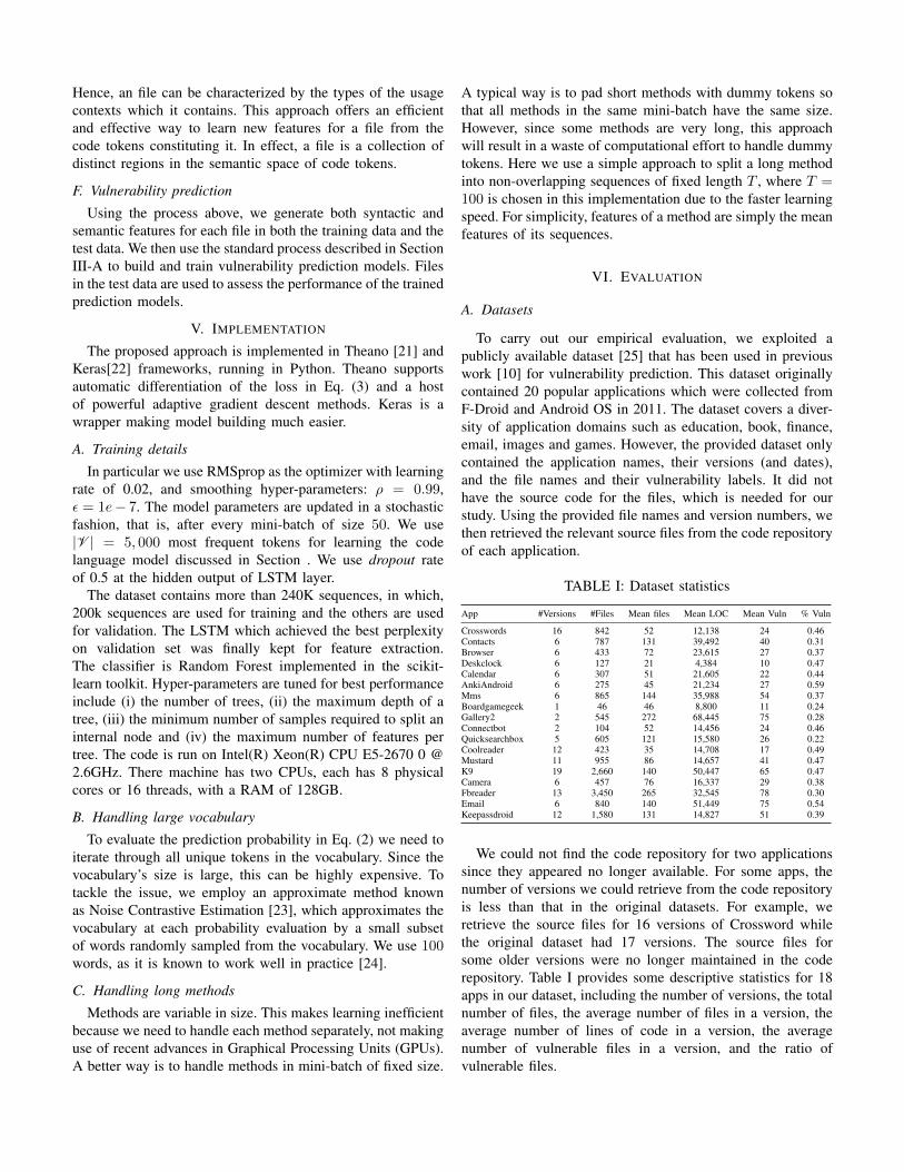
Hence, an file can be characterized by the types of the usagecontexts which it contains. This approach offers an efficientand effective way to learn new features for a file from thecode tokens constituting it. In effect, a file is a collection ofdistinct regions in the semantic space of code tokens.

F. Vulnerability prediction

Using the process above, we generate both syntactic andsemantic features for each file in both the training data and thetest data. We then use the standard process described in SectionIII-A to build and train vulnerability prediction models. Filesin the test data are used to assess the performance of the trainedprediction models.

V. IMPLEMENTATION

The proposed approach is implemented in Theano [21] andKeras[22] frameworks, running in Python. Theano supportsautomatic differentiation of the loss in Eq. (3) and a hostof powerful adaptive gradient descent methods. Keras is awrapper making model building much easier.

A. Training details

In particular we use RMSprop as the optimizer with learningrate of 0.02, and smoothing hyper-parameters: ρ = 0.99,ε = 1e− 7. The model parameters are updated in a stochasticfashion, that is, after every mini-batch of size 50. We use|V | = 5, 000 most frequent tokens for learning the codelanguage model discussed in Section . We use dropout rateof 0.5 at the hidden output of LSTM layer.

The dataset contains more than 240K sequences, in which,200k sequences are used for training and the others are usedfor validation. The LSTM which achieved the best perplexityon validation set was finally kept for feature extraction.The classifier is Random Forest implemented in the scikit-learn toolkit. Hyper-parameters are tuned for best performanceinclude (i) the number of trees, (ii) the maximum depth of atree, (iii) the minimum number of samples required to split aninternal node and (iv) the maximum number of features pertree. The code is run on Intel(R) Xeon(R) CPU E5-2670 0 @2.6GHz. There machine has two CPUs, each has 8 physicalcores or 16 threads, with a RAM of 128GB.

B. Handling large vocabulary

To evaluate the prediction probability in Eq. (2) we need toiterate through all unique tokens in the vocabulary. Since thevocabulary’s size is large, this can be highly expensive. Totackle the issue, we employ an approximate method knownas Noise Contrastive Estimation [23], which approximates thevocabulary at each probability evaluation by a small subsetof words randomly sampled from the vocabulary. We use 100words, as it is known to work well in practice [24].

C. Handling long methods

Methods are variable in size. This makes learning inefficientbecause we need to handle each method separately, not makinguse of recent advances in Graphical Processing Units (GPUs).A better way is to handle methods in mini-batch of fixed size.

A typical way is to pad short methods with dummy tokens sothat all methods in the same mini-batch have the same size.However, since some methods are very long, this approachwill result in a waste of computational effort to handle dummytokens. Here we use a simple approach to split a long methodinto non-overlapping sequences of fixed length T , where T =100 is chosen in this implementation due to the faster learningspeed. For simplicity, features of a method are simply the meanfeatures of its sequences.

VI. EVALUATION

A. Datasets

To carry out our empirical evaluation, we exploited apublicly available dataset [25] that has been used in previouswork [10] for vulnerability prediction. This dataset originallycontained 20 popular applications which were collected fromF-Droid and Android OS in 2011. The dataset covers a diver-sity of application domains such as education, book, finance,email, images and games. However, the provided dataset onlycontained the application names, their versions (and dates),and the file names and their vulnerability labels. It did nothave the source code for the files, which is needed for ourstudy. Using the provided file names and version numbers, wethen retrieved the relevant source files from the code repositoryof each application.

TABLE I: Dataset statistics

App #Versions #Files Mean files Mean LOC Mean Vuln % Vuln

Crosswords 16 842 52 12,138 24 0.46Contacts 6 787 131 39,492 40 0.31Browser 6 433 72 23,615 27 0.37Deskclock 6 127 21 4,384 10 0.47Calendar 6 307 51 21,605 22 0.44AnkiAndroid 6 275 45 21,234 27 0.59Mms 6 865 144 35,988 54 0.37Boardgamegeek 1 46 46 8,800 11 0.24Gallery2 2 545 272 68,445 75 0.28Connectbot 2 104 52 14,456 24 0.46Quicksearchbox 5 605 121 15,580 26 0.22Coolreader 12 423 35 14,708 17 0.49Mustard 11 955 86 14,657 41 0.47K9 19 2,660 140 50,447 65 0.47Camera 6 457 76 16,337 29 0.38Fbreader 13 3,450 265 32,545 78 0.30Email 6 840 140 51,449 75 0.54Keepassdroid 12 1,580 131 14,827 51 0.39

We could not find the code repository for two applicationssince they appeared no longer available. For some apps, thenumber of versions we could retrieve from the code repositoryis less than that in the original datasets. For example, weretrieve the source files for 16 versions of Crossword whilethe original dataset had 17 versions. The source files forsome older versions were no longer maintained in the coderepository. Table I provides some descriptive statistics for 18apps in our dataset, including the number of versions, the totalnumber of files, the average number of files in a version, theaverage number of lines of code in a version, the averagenumber of vulnerable files in a version, and the ratio ofvulnerable files.

B. Research questionsWe followed previous work in vulnerability prediction [10]

and aimed to answer the following standard research questions:1) RQ1. Within-project prediction: Are the automatically

learned features using LSTM suitable for building avulnerability prediction model?To answer this question, we focused on one version (thefirst one) in each application in our dataset. We ran across-fold validation experiments by dividing the filesin each application into 10 folds, each of which havethe approximately same ratio between vulnerable filesand clean files. Each fold is used as the test set and theremaining folds are used for training. As a result, webuilt 10 different prediction models and the performanceindicators are averaged out of the 10 folds.

2) RQ2. Cross-version prediction: How does our pro-posed approach perform in predicting future releases,i.e. when the model is trained using an older version inapplication and tested on a newer version in the sameapplication?In this second experiment, all the files in the first versionof each application are used to train a prediction model,which is then used to predict vulnerability of the files ofall subsequent versions. For example, the first version inthe Crosswords app is used to training and each of theremaining 15 versions is used as a test set.

3) RQ3. Cross-project prediction: Is our approach suit-able for cross-project predictions where the model istrained using a source application and tested on adifferent application?In the third experiment, we used all the files in the firstversion of each project for training a prediction model.This model is then tested on the first version of theremaining applications.

C. BenchmarksWe compare the performance of our approach against the

following benchmarks:Software metrics: Complexity metrics have been exten-

sively used for defect prediction (e.g. [26]) and vulnerabilityprediction (e.g. [8, 27, 28]). This is resulted from the intuitionthat complex code is difficult to understand, maintain and test,and thus has a higher chance of having vulnerabilities thansimple code. We have implemented a vulnerability predictionmodels based on 60 metrics. These features are commonlyused in existing vulnerability prediction models. They covers7 categories: cohesion metrics, complexity metrics, couplingmetrics, documentation metrics, inheritance metrics, code du-plication metrics, and size metrics.

Bag of Words: This technique has been used in previouswork [10], which also consider source code as a special formof text. Hence, it treats a source file as a collection of termsassociated with frequencies. The term frequencies are thefeatures which are used as the predictors for a vulnerabilityprediction model. Lexical analysis is done to source code tobreak it into a vector of code tokens and the frequency of

each token in the file is counted. We also followed previouswork [10] by discretizing the BoW features since they foundthat this method significantly improved the performance ofthe vulnerability prediction models. The discretization processinvolves transforming the numerical BoW features into twobins. If a code token occurs more than a certain threshold(e.g. 5 times) than it is mapped to one bin, otherwise it ismapped to another bin.

Deep Belief Network: Recent work [29] has demonstratedthat Deep Belief Network (DBN) [30] worked well for defectprediction. DBN is a family of stochastic deep neural networkswhich extract multiple layers of data representation. In ourimplementation, DBN takes the word counts per file as inputand produces a latent posterior as output, which is then usedas a new file representation. Since the standard DBN acceptsonly input in the range [0,1], we normalize the word countsby dividing each dimension to its maximum value accrossthe entire training data. The DBN is then built in a stage-wise fashion as follows. At the bottom layer, a RestrictedBoltzmann Machine (RBM) is trained on the normalizedword count. An RBM is a special two-layer neural networkwith binary neurons. Following the standard practice in theliterature, the RBM is trained using Contrastive Divergence[30]. After the first RBM is trained, its posterior is used as theinput for the next RBM, and the training is repeated. Finally,the two RBMs are stacked on top of each other to form a DBNwith two hidden layers. The posterior of the second RBM isused as the new file representation. In our implementation, thetwo hidden layers have the size of 500 and 128, respectively.

To enable a fair comparison, we used the same classifierfor our prediction models and all the benchmarks. We choseRandom Forests (RF), an ensemble method which combinesthe estimates from multiple estimators since it is one ofthe most effective classifier for vulnerability prediction [10].We employed the standard Precision, Recall, and F-measure,which has been widely-used in the literature (e.g. [5, 8, 10,28]) for evaluating the predictive performance of vulnerabilityprediction models built using the three above benchmarks andour approach.

D. Results

1) Learned code token semantics: An important part ofour approach is learning the semantics of code tokens usingthe context of its usage through LSTM. Figure 7 show thetop 2,000 frequent code tokens used in our dataset. Theywere automatically grouped in 10 clusters (using K-meansclustering) based on their token states learned through LSTM.Recall that these clusters are the basis for us to construct acodebook (discussed in Section IV-E). We used t-distributedstochastic neighbor embedding (t-SNE) [31] to display high-dimensional vectors in two dimensions. We show here somerepresentative code tokens from some clusters for a briefillustration. Code tokens that are semantically related aregrouped in the same cluster. For example, code tokens relatedto exceptions such as IllegalArgumentException, FileNot-FoundException, and NoSuchMethodException are grouped

TABLE II: Within-project results (RQ1) for the three benchmarks and three variations of our approach. “Joint features” indicatesthe use of both syntactic features and semantic features.

Application Software metrics Bag-of-Words Deep Belief Network Syntactic features Semantic features Joint featuresP R F P R F P R F P R F P R F P R F

AnkiAndroid 0.62 0.65 0.61 1.00 0.94 0.96 1.00 0.94 0.96 1.00 1.00 1.00 1.00 0.94 0.96 1.00 0.94 0.96Boardgamegeek 0.18 0.35 0.23 0.95 1.00 0.97 0.95 1.00 0.97 0.95 0.95 0.93 0.90 0.90 0.90 0.90 0.90 0.90Browser 0.65 0.60 0.62 0.96 1.00 0.98 0.96 1.00 0.98 1.00 1.00 1.00 0.96 1.00 0.98 0.96 1.00 0.98Calendar 0.52 0.43 0.45 0.89 0.80 0.83 1.00 0.91 0.94 1.00 1.00 1.00 0.96 0.94 0.94 1.00 1.00 1.00Camera 0.72 0.81 0.73 0.82 0.92 0.86 0.83 0.93 0.87 0.88 1.00 0.93 0.92 0.98 0.94 0.92 0.98 0.94Connectbot 0.65 0.73 0.64 0.97 0.90 0.91 0.92 0.90 0.88 1.00 0.97 0.98 0.93 0.93 0.93 0.97 0.93 0.93Contacts 0.72 0.72 0.71 0.94 0.88 0.89 0.92 0.81 0.83 0.96 0.94 0.95 0.89 0.94 0.89 0.87 0.97 0.90Coolreader 0.55 0.70 0.60 1.00 1.00 1.00 1.00 1.00 1.00 1.00 0.94 0.96 1.00 0.94 0.96 1.00 0.94 0.96Crosswords 0.55 0.57 0.55 0.89 0.89 0.89 0.89 0.89 0.89 0.89 0.89 0.89 0.89 0.83 0.85 0.89 0.83 0.85Deskclock 0.30 0.20 0.23 0.92 0.92 0.89 0.83 0.92 0.83 1.00 1.00 1.00 1.00 0.92 0.94 1.00 0.92 0.94Email 0.83 0.84 0.82 0.92 0.93 0.92 0.96 0.94 0.94 0.93 0.95 0.93 0.95 0.90 0.92 0.94 0.93 0.93Fbreader 0.60 0.52 0.55 0.78 0.88 0.81 0.81 0.85 0.82 0.83 0.82 0.82 0.85 0.83 0.84 0.82 0.86 0.83Gallery2 0.62 0.60 0.57 0.80 0.91 0.84 0.75 0.87 0.78 0.83 0.88 0.84 0.83 0.87 0.84 0.80 0.89 0.83K9 0.73 0.82 0.76 0.94 0.88 0.89 0.96 0.87 0.90 0.89 1.00 0.94 0.88 0.97 0.91 0.88 0.98 0.92Keepassdroid 0.69 0.75 0.71 0.91 0.88 0.88 0.85 0.90 0.87 0.93 0.97 0.94 0.90 0.91 0.89 0.88 0.89 0.88Mms 0.78 0.60 0.67 0.86 0.85 0.85 0.84 0.85 0.84 0.87 0.85 0.85 0.87 0.88 0.87 0.87 0.92 0.89Mustard 0.81 0.68 0.72 0.94 0.93 0.93 0.94 0.87 0.89 0.96 0.99 0.97 0.97 0.93 0.94 0.95 0.99 0.96Quicksearchbox 0.60 0.42 0.43 0.84 0.90 0.83 0.83 0.90 0.84 0.93 0.90 0.88 0.89 0.77 0.82 0.89 0.79 0.82

Average 0.62 0.61 0.59 0.91 0.91 0.90 0.90 0.91 0.89 0.94 0.95 0.93 0.92 0.91 0.91 0.92 0.93 0.91

in one cluster. This indicates, to some extent, that the learnedtoken states effectively capture the semantic relations betweencode tokens, which is useful for us to learn both syntactic andsemantic features later.

20 15 10 5 0 5 10 15 2020

15

10

5

0

5

10

15

20onCreate

(

SQLException

.about

openDatabasenull

TAG

queryScalar

Cursor

longscalar

trythrow

finally

>queryColumn

,

String

do

int

Exception

KEY_CHECK_URI

Editor

Intent

File

MODE_READ_ONLY

FileNotFoundException getTypeinsert

queryupdate

onCheckedChanged

onClick

case

ease1

VIBRATOR_SERVICE

ease2ease3ease4

AnkidroidApp

>=

<NUM>

-

DECK_LOADED

DECK_NOT_LOADED

DECK_EMPTY

OPT_DB

IOException

MENU_PREFERENCES

MENU_DECKOPTS

MENU_SUSPEND

MENU_EDIT

RESULT_OK

/:

Fact

<STR>

spaceUntilabsPath

FINISHED

trueEQUALJSONException

NoSuchMethodException

IllegalArgumentException

IllegalAccessException

Fig. 7: Top 2,000 frequent code tokens were automaticallygrouped into clusters (each cluster has a distinct color)

2) Within-project prediction (RQ1): We experimented witha number of variations of our approach by varying the poolingtechniques (mean pooling and standard deviation pooling) andthe use of syntactic and semantic features. Table II reportsthe precision, recall and F-measure for the three benchmarks(software metrics, Bag-of-Words, and Deep Belief Network)and three variations of our approach: using only syntacticfeatures, using only semantic features, and using a joint setof both features types. Note that both the syntactic featureoption and and the joint feature option we reported here usedmean pooling for generating method features and standarddeviation pooling for generating syntactic file features. The fullreport which contains the results for all variations of poolingis available at https://goo.gl/OnRnPp.

Our approach obtained a strong result: in all 18 applications,they all achieved more than 80% in precision, recall, andF-measure (see Table II). Among the three variation of ourapproach, using only syntactic features appeared to be thebest option for vulnerable prediction within one version ofa project. This option delivered the highest precision, recalland F-measure averaging across 18 applications. This result isconsistent with our underlying theory that syntactic featuresare project-specific and are thus useful for within-projectprediction. Our approach outperforms the three benchmarksto varying extents. The syntactic feature option offered 58%F-measure improvement over the software metrics approach.Both Bag-of-Words (BoW) and Deep Belief Network ap-proaches also achieved very good results (on average 89–90%F-measure) – which is consistent with the findings in previouswork [10] in case of BoW. Hence, comparing against thesetwo benchmarks, the improvement brought by our approach issmall (approximately 3% in F-measure).

3) Cross-version prediction (RQ2): Table III reports theresults in a cross-version setting where a prediction modelwas trained using the first version of an application andtested using the subsequent versions of the same applica-tions. Our approach again slightly outperforms the BoW andDBN benchmarks. Among the three variations, using semanticfeatures (alone or joint with syntactic features) becomes thebest options. This is because semantic measures improvethe generalization of the prediction models, which becomesslightly more useful in cross-version settings.

4) Cross-project prediction (RQ3): This experiment fol-lowed the setup in previous work [10]. We first built 18prediction models, each of which use the first version of eachapplication for training. Each model was then tested usingthe first version of the other 17 applications. We ran thisexperiment with the three benchmarks and variations of ourapproach. We used the same baseline as in previous work

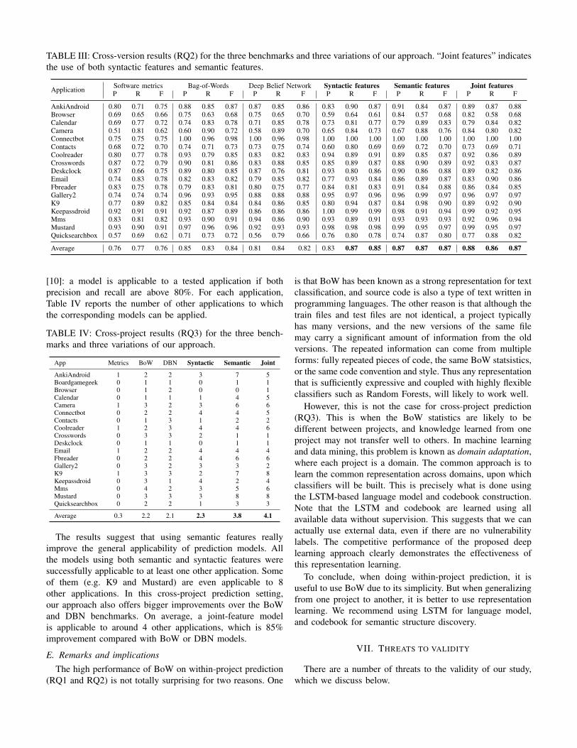
TABLE III: Cross-version results (RQ2) for the three benchmarks and three variations of our approach. “Joint features” indicatesthe use of both syntactic features and semantic features.

Application Software metrics Bag-of-Words Deep Belief Network Syntactic features Semantic features Joint featuresP R F P R F P R F P R F P R F P R F

AnkiAndroid 0.80 0.71 0.75 0.88 0.85 0.87 0.87 0.85 0.86 0.83 0.90 0.87 0.91 0.84 0.87 0.89 0.87 0.88Browser 0.69 0.65 0.66 0.75 0.63 0.68 0.75 0.65 0.70 0.59 0.64 0.61 0.84 0.57 0.68 0.82 0.58 0.68Calendar 0.69 0.77 0.72 0.74 0.83 0.78 0.71 0.85 0.78 0.73 0.81 0.77 0.79 0.89 0.83 0.79 0.84 0.82Camera 0.51 0.81 0.62 0.60 0.90 0.72 0.58 0.89 0.70 0.65 0.84 0.73 0.67 0.88 0.76 0.84 0.80 0.82Connectbot 0.75 0.75 0.75 1.00 0.96 0.98 1.00 0.96 0.98 1.00 1.00 1.00 1.00 1.00 1.00 1.00 1.00 1.00Contacts 0.68 0.72 0.70 0.74 0.71 0.73 0.73 0.75 0.74 0.60 0.80 0.69 0.69 0.72 0.70 0.73 0.69 0.71Coolreader 0.80 0.77 0.78 0.93 0.79 0.85 0.83 0.82 0.83 0.94 0.89 0.91 0.89 0.85 0.87 0.92 0.86 0.89Crosswords 0.87 0.72 0.79 0.90 0.81 0.86 0.83 0.88 0.85 0.85 0.89 0.87 0.88 0.90 0.89 0.92 0.83 0.87Deskclock 0.87 0.66 0.75 0.89 0.80 0.85 0.87 0.76 0.81 0.93 0.80 0.86 0.90 0.86 0.88 0.89 0.82 0.86Email 0.74 0.83 0.78 0.82 0.83 0.82 0.79 0.85 0.82 0.77 0.93 0.84 0.86 0.89 0.87 0.83 0.90 0.86Fbreader 0.83 0.75 0.78 0.79 0.83 0.81 0.80 0.75 0.77 0.84 0.81 0.83 0.91 0.84 0.88 0.86 0.84 0.85Gallery2 0.74 0.74 0.74 0.96 0.93 0.95 0.88 0.88 0.88 0.95 0.97 0.96 0.96 0.99 0.97 0.96 0.97 0.97K9 0.77 0.89 0.82 0.85 0.84 0.84 0.84 0.86 0.85 0.80 0.94 0.87 0.84 0.98 0.90 0.89 0.92 0.90Keepassdroid 0.92 0.91 0.91 0.92 0.87 0.89 0.86 0.86 0.86 1.00 0.99 0.99 0.98 0.91 0.94 0.99 0.92 0.95Mms 0.83 0.81 0.82 0.93 0.90 0.91 0.94 0.86 0.90 0.93 0.89 0.91 0.93 0.93 0.93 0.92 0.96 0.94Mustard 0.93 0.90 0.91 0.97 0.96 0.96 0.92 0.93 0.93 0.98 0.98 0.98 0.99 0.95 0.97 0.99 0.95 0.97Quicksearchbox 0.57 0.69 0.62 0.71 0.73 0.72 0.56 0.79 0.66 0.76 0.80 0.78 0.74 0.87 0.80 0.77 0.88 0.82

Average 0.76 0.77 0.76 0.85 0.83 0.84 0.81 0.84 0.82 0.83 0.87 0.85 0.87 0.87 0.87 0.88 0.86 0.87

[10]: a model is applicable to a tested application if bothprecision and recall are above 80%. For each application,Table IV reports the number of other applications to whichthe corresponding models can be applied.

TABLE IV: Cross-project results (RQ3) for the three bench-marks and three variations of our approach.

App Metrics BoW DBN Syntactic Semantic Joint

AnkiAndroid 1 2 2 3 7 5Boardgamegeek 0 1 1 0 1 1Browser 0 1 2 0 0 1Calendar 0 1 1 1 4 5Camera 1 3 2 3 6 6Connectbot 0 2 2 4 4 5Contacts 0 1 3 1 2 2Coolreader 1 2 3 4 4 6Crosswords 0 3 3 2 1 1Deskclock 0 1 1 0 1 1Email 1 2 2 4 4 4Fbreader 0 2 2 4 6 6Gallery2 0 3 2 3 3 2K9 1 3 3 2 7 8Keepassdroid 0 3 1 4 2 4Mms 0 4 2 3 5 6Mustard 0 3 3 3 8 8Quicksearchbox 0 2 2 1 3 3

Average 0.3 2.2 2.1 2.3 3.8 4.1

The results suggest that using semantic features reallyimprove the general applicability of prediction models. Allthe models using both semantic and syntactic features weresuccessfully applicable to at least one other application. Someof them (e.g. K9 and Mustard) are even applicable to 8other applications. In this cross-project prediction setting,our approach also offers bigger improvements over the BoWand DBN benchmarks. On average, a joint-feature modelis applicable to around 4 other applications, which is 85%improvement compared with BoW or DBN models.

E. Remarks and implicationsThe high performance of BoW on within-project prediction

(RQ1 and RQ2) is not totally surprising for two reasons. One

is that BoW has been known as a strong representation for textclassification, and source code is also a type of text written inprogramming languages. The other reason is that although thetrain files and test files are not identical, a project typicallyhas many versions, and the new versions of the same filemay carry a significant amount of information from the oldversions. The repeated information can come from multipleforms: fully repeated pieces of code, the same BoW statsistics,or the same code convention and style. Thus any representationthat is sufficiently expressive and coupled with highly flexibleclassifiers such as Random Forests, will likely to work well.

However, this is not the case for cross-project prediction(RQ3). This is when the BoW statistics are likely to bedifferent between projects, and knowledge learned from oneproject may not transfer well to others. In machine learningand data mining, this problem is known as domain adaptation,where each project is a domain. The common approach is tolearn the common representation across domains, upon whichclassifiers will be built. This is precisely what is done usingthe LSTM-based language model and codebook construction.Note that the LSTM and codebook are learned using allavailable data without supervision. This suggests that we canactually use external data, even if there are no vulnerabilitylabels. The competitive performance of the proposed deeplearning approach clearly demonstrates the effectiveness ofthis representation learning.

To conclude, when doing within-project prediction, it isuseful to use BoW due to its simplicity. But when generalizingfrom one project to another, it is better to use representationlearning. We recommend using LSTM for language model,and codebook for semantic structure discovery.

VII. THREATS TO VALIDITY

There are a number of threats to the validity of our study,which we discuss below.

Construct validity: We mitigated the construct validityconcerns by using a publicly available dataset that has beenused in previous work [10]. The dataset contains real Androidapplications and vulnerability labels of the files in those appli-cations. The original dataset did not unfortunately contain thesource files. However, we have carefully used the information(e.g. application details, version numbers and date) providedwith the dataset to retrieve the relevant source files from thecode repository of those applications.

Conclusion validity: We tried to minimize threats to con-clusion validity by using standard performance measures forvulnerability prediction [8, 10, 28, 32]. We however acknowl-edge that a number of statistical tests [33] can be applied toverify the statistical significance of our conclusions. Althoughwe have not seen those statistical tests being used in previouswork in vulnerability prediction, we plan to do this investiga-tion in our future work.

Internal validity: The dataset we used contains vulnerabil-ity labels only for Java source files. In practice, other files (e.g.XML manifest files) may contain security information suchas access rights. Another threat concerns the cross-versionprediction where we replicated the experiment done in [10]and allowed that the exactly same files might be presentbetween versions. This might have inflated the results, butall the prediction models which we compared against in ourexperiment benefit from this.

External validity: We have considered a large numberof applications which differ significantly in size, complexity,domain, popularity and revision history. We however acknowl-edge that our data set may not be representative of all kindsof Android applications. Further investigation to confirm ourfindings for other Android applications as well as other typesof applications such as web applications and applicationswritten in other programming languages such as PhP and C++.

VIII. RELATED WORK

Machine learning techniques have been widely used tobuild vulnerability prediction models. Early approaches (e.g.[27]) employed complexity metrics such as (e.g. McCabe’scyclomatic complexity, nesting complexity, and size) as thepredictors. Later approaches enriched this software metricfeature set with coupling and cohesion metrics (e.g. [28]),code churn and developer activity metrics (e.g. [8])), anddependencies and organizational measures (e.g. [5]). Those ap-proaches require knowledgeable domain experts to determinethe metrics that are used as predictors for vulnerability.

Recent approaches treat source code as another form of textand leverage text mining techniques to extract the featuresfor building vulnerability prediction models. The work in [10]used the Bag-of-Words representation in which a source codefile is viewed as a set of terms with associated frequen-cies. They then used the term-frequencies as the features forpredicting vulnerability. The BoW approach eliminates theneed for manually designing the features. BoW models alsoproduced higher recall than software metric models for PHPapplications [32]. However, the BoW approaches carries the

inherent limitation of BoW in which syntactic informationsuch as code order is disregarded.

Predicting vulnerabilities is related to software defect pre-diction. The study in [34] found that some defect predictionmodels can be adapted for vulnerability prediction. While codemetrics were commonly used as features for building defectprediction models [26], various other metrics have also beenemployed such as change-related metrics [35, 36], developer-related metrics [37], organization metrics [38], and changeprocess metrics [39]. Recently, a number of approaches (e.g.[29, 40]) have leveraged a deep learning model called DeepBelief Network [41] to automatically learn features for defectprediction.

Deep learning has recently attracted increasing interests insoftware engineering. The work in [42] proposes generic deeplearning framework based on LSTM for modeling softwareand its development process. The work in [17] demonstratedthe effectiveness of using recurrent neural networks (RNN)to model source code. Their later work [43] extended theseRNN models for detecting code clones. The work in [44] usesa special RNN Encoder–Decoder, which consists of an encoderRNN to process the input sequence and a decoder RNN withattention to generate the output sequence, to generate APIusage sequences for a given API-related natural languagequery. The work in [45] also uses RNN Encoder–Decoderbut for fixing common errors in C programs. The work [24]showed that LSTM is even more effective in code modeling,which inspired us to use it for learning vulnerability features.The work in [46] uses Convolutional Neural Networks (CNN)[47] for bug localization.

IX. CONCLUSIONS AND FUTURE WORK

This paper proposes to leverage Long-Short Term Memory,a representation deep learning model, to automatically learnfeatures directly from source code for vulnerability prediction.The learned syntactic features capture the sequential struc-ture in code at the method level, while semantic featurescharacterize a source code file by usage contexts of its codetokens. We performed an evaluation on 18 Android applica-tions from a public dataset provided in previous work [10].The results for within-project prediction demonstrate that theautomatically learned features significantly outperforms thetraditional software metrics approach (58% improvement onaverage), and offers a small improvement (3% on average)over the Bag-of-Word approach and another deep learningapproach (Deep Belief Network). For cross-project prediction,the results suggest that our approach is clearly superior to thesestate-of-the-art techniques (85% improvement on average).

Our future work involves applying the proposed approachto other types of applications (e.g. Web applications) andprogramming languages (e.g. PHP or C++) where vulnerabilitydatasets are available. We also aim to leverage our approachto learn features for predicting vulnerabilities at the methodand code change levels. In addition, we plan to explore howour approach can be extended to predicting general defects andsafety-critical hazards in code. Finally, our future investigation

involves building a fully end-to-end prediction system fromraw input data (code tokens) to vulnerability outcomes.

ACKNOWLEDGEMENT

The paper is supported by Samsung 2016 Global ResearchOutreach Program (GRO) entitled “Predicting hazardous soft-ware components using deep learning”.

REFERENCES

[1] R. Hackett, “On Heartbleed’s anniversary, 3 of 4 big companiesare still vulnerable,” Fortunue, http://fortune.com/2015/04/07/heartbleed-anniversary-vulnerable, April 2015.

[2] McAfee, C. for Strategic, and I. Studies, “Net Losses: Estimating theGlobal Cost of Cybercrime,” June 2014.

[3] C. Ventures, “Cybersecurity market report,”http://cybersecurityventures.com/cybersecurity-market-report, Accessedon 01 May 2017, March 2017.

[4] C. Williams, “Anatomy of OpenSSL’s Heartbleed:Just four bytes trigger horror bug,” The Register,http://www.theregister.co.uk/2014/04/09/heartbleed explained,Accessed on 01 May 2017, April 2014.

[5] T. Zimmermann, N. Nagappan, and L. Williams, “Searching for aneedle in a haystack: Predicting security vulnerabilities for windowsvista,” in Proceedings of the 2010 Third International Conferenceon Software Testing, Verification and Validation, ser. ICST ’10.Washington, DC, USA: IEEE Computer Society, 2010, pp. 421–428.[Online]. Available: http://dx.doi.org/10.1109/ICST.2010.32

[6] A. Austin and L. Williams, “One technique is not enough: Acomparison of vulnerability discovery techniques,” in Proceedings ofthe 2011 International Symposium on Empirical Software Engineeringand Measurement, ser. ESEM ’11. Washington, DC, USA: IEEEComputer Society, 2011, pp. 97–106. [Online]. Available: http://dx.doi.org/10.1109/ESEM.2011.18

[7] M. Ceccato and R. Scandariato, “Static analysis and penetrationtesting from the perspective of maintenance teams,” in Proceedingsof the 10th ACM/IEEE International Symposium on EmpiricalSoftware Engineering and Measurement, ser. ESEM ’16. NewYork, NY, USA: ACM, 2016, pp. 25:1–25:6. [Online]. Available:http://doi.acm.org/10.1145/2961111.2962611

[8] Y. Shin, A. Meneely, L. Williams, and J. A. Osborne, “Evaluatingcomplexity, code churn, and developer activity metrics as indicatorsof software vulnerabilities,” IEEE Trans. Softw. Eng., vol. 37, no. 6,pp. 772–787, Nov. 2011. [Online]. Available: http://dx.doi.org/10.1109/TSE.2010.81

[9] T. Zimmermann, N. Nagappan, H. Gall, E. Giger, and B. Murphy,“Cross-project defect prediction: A large scale experiment on data vs.domain vs. process,” in Proceedings of the the 7th Joint Meeting ofthe European Software Engineering Conference and the ACM SIGSOFTSymposium on The Foundations of Software Engineering, ser. ESEC/FSE’09. New York, NY, USA: ACM, 2009, pp. 91–100.

[10] R. Scandariato, J. Walden, A. Hovsepyan, and W. Joosen, “Predictingvulnerable software components via text mining.” IEEE Trans. SoftwareEng., vol. 40, no. 10, pp. 993–1006, 2014. [Online]. Available:http://dblp.uni-trier.de/db/journals/tse/tse40.html#ScandariatoWHJ14

[11] Y. LeCun, Y. Bengio, and G. Hinton, “Deep learning,” Nature, vol. 521,no. 7553, pp. 436–444, 2015.

[12] S. Hochreiter and J. Schmidhuber, “Long short-term memory,” Neuralcomputation, vol. 9, no. 8, pp. 1735–1780, 1997.

[13] D. Mohindra, “SEI CERT Oracle Coding Standard for Java,”https://www.securecoding.cert.org/confluence/display/java/LCK08-J.+Ensure+actively+held+locks+are+released+on+exceptional+conditions,Accessed on 01 May 2017.

[14] S. Hochreiter, Y. Bengio, P. Frasconi, and J. Schmidhuber, “Gradientflow in recurrent nets: the difficulty of learning long-term dependencies,”2001.

[15] F. A. Gers, J. Schmidhuber, and F. Cummins, “Learning to forget:Continual prediction with lstm,” Neural computation, vol. 12, no. 10,pp. 2451–2471, 2000.

[16] JavaParser, “JavaParser,” http://javaparser.org, Accessed on 01 Feb 2017.

[17] M. White, C. Vendome, M. Linares-Vasquez, and D. Poshyvanyk,“Toward deep learning software repositories,” in Proceedings of the 12thWorking Conference on Mining Software Repositories, ser. MSR ’15.Piscataway, NJ, USA: IEEE Press, 2015, pp. 334–345.

[18] C. L. Giles, S. Lawrence, and A. C. Tsoi, “Noisy time series predictionusing recurrent neural networks and grammatical inference,” Machinelearning, vol. 44, no. 1, pp. 161–183, 2001.

[19] M. Baroni, G. Dinu, and G. Kruszewski, “Don’t count, predict! a sys-tematic comparison of context-counting vs. context-predicting semanticvectors.” in ACL (1), 2014, pp. 238–247.

[20] D. G. Lowe, “Object recognition from local scale-invariant features,” inComputer vision, 1999. The proceedings of the seventh IEEE interna-tional conference on, vol. 2. Ieee, 1999, pp. 1150–1157.

[21] Theano, “Theano,” http://deeplearning.net/software/theano/, Accessedon 01 May 2017.

[22] Keras, “Keras: Deep Learning library for Theano and TensorFlow,”https://keras.io/, Accessed on 01 May 2017.

[23] M. U. Gutmann and A. Hyvarinen, “Noise-contrastive estimation ofunnormalized statistical models, with applications to natural imagestatistics,” Journal of Machine Learning Research, vol. 13, no. Feb,pp. 307–361, 2012.

[24] H. K. Dam, T. Tran, and T. Pham, “A deep language model forsoftware code,” in Workshop on Naturalness of Software (NL+SE), co-located with the 24th ACM SIGSOFT International Symposium on theFoundations of Software Engineering (FSE), 2016.

[25] R. Scandariato, J. Walden, A. Hovsepyan, and W. Joosen, “Android studydataset,” https://sites.google.com/site/textminingandroid, Accessed on 15Jan 2017, 2014.

[26] T. Hall, S. Beecham, D. Bowes, D. Gray, and S. Counsell, “Asystematic literature review on fault prediction performance in softwareengineering,” IEEE Trans. Softw. Eng., vol. 38, no. 6, pp. 1276–1304,Nov. 2012. [Online]. Available: http://dx.doi.org/10.1109/TSE.2011.103

[27] Y. Shin and L. Williams, “An empirical model to predict securityvulnerabilities using code complexity metrics,” in Proceedingsof the Second ACM-IEEE International Symposium on EmpiricalSoftware Engineering and Measurement, ser. ESEM ’08. NewYork, NY, USA: ACM, 2008, pp. 315–317. [Online]. Available:http://doi.acm.org/10.1145/1414004.1414065

[28] I. Chowdhury and M. Zulkernine, “Using complexity, coupling, andcohesion metrics as early indicators of vulnerabilities,” J. Syst.Archit., vol. 57, no. 3, pp. 294–313, Mar. 2011. [Online]. Available:http://dx.doi.org/10.1016/j.sysarc.2010.06.003

[29] S. Wang, T. Liu, and L. Tan, “Automatically learning semanticfeatures for defect prediction,” in Proceedings of the 38th InternationalConference on Software Engineering, ser. ICSE ’16. New York,NY, USA: ACM, 2016, pp. 297–308. [Online]. Available: http://doi.acm.org/10.1145/2884781.2884804

[30] G. Hinton and R. Salakhutdinov, “Reducing the dimensionality of datawith neural networks,” Science, vol. 313, no. 5786, pp. 504–507, 2006.

[31] L. van der Maaten and G. Hinton, “Visualizing data using t-SNE,”Journal of Machine Learning Research, vol. 9, no. 2579-2605, p. 85,2008.

[32] J. Walden, J. Stuckman, and R. Scandariato, “Predicting vulnerablecomponents: Software metrics vs text mining,” in Proceedingsof the 2014 IEEE 25th International Symposium on SoftwareReliability Engineering, ser. ISSRE ’14. Washington, DC, USA:IEEE Computer Society, 2014, pp. 23–33. [Online]. Available:http://dx.doi.org/10.1109/ISSRE.2014.32

[33] A. Arcuri and L. Briand, “A Hitchhiker’s guide to statistical tests forassessing randomized algorithms in software engineering,” SoftwareTesting, Verification and Reliability, vol. 24, no. 3, pp. 219–250, 2014.[Online]. Available: http://dx.doi.org/10.1002/stvr.1486

[34] Y. Shin and L. Williams, “Can traditional fault prediction models beused for vulnerability prediction?” Empirical Software Engineering,vol. 18, no. 1, pp. 25–59, 2013. [Online]. Available: http://dx.doi.org/10.1007/s10664-011-9190-8

[35] R. Moser, W. Pedrycz, and G. Succi, “A comparative analysisof the efficiency of change metrics and static code attributesfor defect prediction,” in Proceedings of the 30th InternationalConference on Software Engineering, ser. ICSE ’08. New York,NY, USA: ACM, 2008, pp. 181–190. [Online]. Available: http://doi.acm.org/10.1145/1368088.1368114

[36] N. Nagappan and T. Ball, “Use of relative code churn measuresto predict system defect density,” in Proceedings of the 27th

International Conference on Software Engineering, ser. ICSE ’05.New York, NY, USA: ACM, 2005, pp. 284–292. [Online]. Available:http://doi.acm.org/10.1145/1062455.1062514

[37] M. Pinzger, N. Nagappan, and B. Murphy, “Can developer-modulenetworks predict failures?” in Proceedings of the 16th ACM SIGSOFTInternational Symposium on Foundations of Software Engineering, ser.SIGSOFT ’08/FSE-16. New York, NY, USA: ACM, 2008, pp. 2–12.[Online]. Available: http://doi.acm.org/10.1145/1453101.1453105

[38] N. Nagappan, B. Murphy, and V. Basili, “The influence of organizationalstructure on software quality: An empirical case study,” in Proceedingsof the 30th International Conference on Software Engineering, ser.ICSE ’08. New York, NY, USA: ACM, 2008, pp. 521–530. [Online].Available: http://doi.acm.org/10.1145/1368088.1368160

[39] A. E. Hassan, “Predicting faults using the complexity of codechanges,” in Proceedings of the 31st International Conference onSoftware Engineering, ser. ICSE ’09. Washington, DC, USA:IEEE Computer Society, 2009, pp. 78–88. [Online]. Available:http://dx.doi.org/10.1109/ICSE.2009.5070510

[40] X. Yang, D. Lo, X. Xia, Y. Zhang, and J. Sun, “Deep learningfor just-in-time defect prediction,” in Proceedings of the 2015 IEEEInternational Conference on Software Quality, Reliability and Security,ser. QRS ’15. Washington, DC, USA: IEEE Computer Society, 2015,pp. 17–26. [Online]. Available: http://dx.doi.org/10.1109/QRS.2015.14

[41] G. Hinton and R. Salakhutdinov, “Reducing the dimensionality of datawith neural networks,” Science, vol. 313, no. 5786, pp. 504 – 507, 2006.

[42] H. K. Dam, T. Tran, J. Grundy, and A. Ghose, “DeepSoft: A vision fora deep model of software,” in Proceedings of the 24th ACM SIGSOFTInternational Symposium on Foundations of Software Engineering, ser.FSE ’16. ACM, To Appear., 2016.

[43] M. White, M. Tufano, C. Vendome, and D. Poshyvanyk, “Deeplearning code fragments for code clone detection,” in Proceedings ofthe 31st IEEE/ACM International Conference on Automated SoftwareEngineering, ser. ASE 2016. New York, NY, USA: ACM, 2016, pp. 87–98. [Online]. Available: http://doi.acm.org/10.1145/2970276.2970326

[44] X. Gu, H. Zhang, D. Zhang, and S. Kim, “Deep api learning,” inProceedings of the 2016 24th ACM SIGSOFT International Symposiumon Foundations of Software Engineering, ser. FSE 2016. NewYork, NY, USA: ACM, 2016, pp. 631–642. [Online]. Available:http://doi.acm.org/10.1145/2950290.2950334

[45] R. Gupta, S. Pal, A. Kanade, and S. Shevade, “Deepfix: Fixing commonC language errors by deep learning,” in Proceedings of the Thirty-FirstAAAI Conference on Artificial Intelligence, February 4-9, 2017, SanFrancisco, California, USA. AAAI Press, 2017, pp. 1345–1351.[Online]. Available: http://aaai.org/ocs/index.php/AAAI/AAAI17/paper/view/14603

[46] X. Huo, M. Li, and Z.-H. Zhou, “Learning unified features fromnatural and programming languages for locating buggy source code,”in Proceedings of the Twenty-Fifth International Joint Conference onArtificial Intelligence, ser. IJCAI’16. AAAI Press, 2016, pp. 1606–1612. [Online]. Available: http://dl.acm.org/citation.cfm?id=3060832.3060845

[47] Y. L. Cun, B. Boser, J. S. Denker, R. E. Howard, W. Habbard, L. D.Jackel, and D. Henderson, “Advances in neural information processingsystems 2,” D. S. Touretzky, Ed. San Francisco, CA, USA: MorganKaufmann Publishers Inc., 1990, ch. Handwritten Digit Recognitionwith a Back-propagation Network, pp. 396–404. [Online]. Available:

http://dl.acm.org/citation.cfm?id=109230.109279