Embed Size (px)
Citation preview

UNIVERSITÉ DE MONTRÉAL
AUTOMATIC DATA GENERATION FOR MC/DC
TEST CRITERION USING METAHEURISTIC
ALGORITHMS
ZEINA AWEDIKIAN
DÉPARTEMENT DE GÉNIE INFORMATIQUE ET GÉNIE LOGICIEL
ÉCOLE POLYTECHNIQUE DE MONTRÉAL
MÉMOIRE PRÉSENTÉ EN VUE DE L‟OBTENTION
DU DIPLÔME DE MAÎTRISE ÈS SCIENCES APPLIQUÉES
(GÉNIE INFORMATIQUE)
AVRIL 2009
© Zeina Awedikian, 2009.
UNIVERSITÉ DE MONTRÉAL
ÉCOLE POLYTECHNIQUE DE MONTRÉAL
Ce mémoire intitulé :
AUTOMATIC DATA GENERATION FOR MC/DC TEST CRITERION USING
METAHEURISTIC ALGORITHMS
présenté par : AWEDIKIAN Zeina
en vue de l‟obtention du diplôme de : Maîtrise ès sciences appliquées
a été dûment accepté par le jury d‟examen constitué de :
M. SAMUEL Pierre, Ph.D., président
M. ANTONIOL Giuliano, Ph.D., membre et directeur de recherche
M. GUÉHÉNEUC Yann-Gaêl, Doct., membre

iii
To my parents, Souraya et Avedis, Thank you.

iv
Acknowledgment
I thank Dr. Giuliano Antoniol for his infinite help throughout my masters. It is
due to his continual presence, his perseverance and his encouragement that I was able to
successfully complete my degree. I am also grateful to him to have me introduced to the
vast world of software testing.

v
Résumé
Le test de logiciel a traditionnellement été l'une des principales techniques
contribuant à la haute fiabilité et à la qualité des logiciels. Les activités de test
consomment environ 50% des ressources de développement de logiciel, ainsi toute
technique visant à réduire les coûts du test est susceptible de réduire le coût total de
développement du logiciel. Le test complet d‟un logiciel est souvent impossible à
réaliser à cause des exécutions infinies nécessaires pour effectuer le test et le prix élevé
par rapport aux limitations du budget.
Les systèmes informatiques de fiabilité élevée sont souvent des systèmes
appartenant aux domaines réglementés tels que le domaine aérospatial et le domaine
médical. Dans de tels domaines, l‟assurance de la qualité et les activités de test de
logiciel sont imposées par la loi ou exigées par des normes obligatoires, telles que le
DO-178B, DO-254, EN-50128, IEEE/EIA 12207, ou ISO/IEC i2207. Ces normes et
règlements imposent normalement des activités de vérification et de validation, ainsi
qu‟ils spécifient les critères de test exigés.
Proposé par la NASA en 1994, la couverture modifiée des décisions et des
conditions (MC/DC) est une stratégie de test requise, entre autres, par le RTCA DO-
178B. MC/DC est un critère de test en boîte blanche qui vise à prouver que chacune des
clauses (expression booléenne ne contenant aucun opérateur logique tel que le z < x +
y) impliquée dans une décision influence correctement la valeur de cette décision. Le
critère MC/DC englobe d'autres critères structurels bien connus tels que la couverture
des instructions et des décisions.
Le travail présenté dans se mémoire applique des techniques d‟optimisation de la
recherche au problème du test. Nous explorons la façon d‟intégrer la distance des
branches, les dépendances de contrôles et les dépendances de données dans la recherche
pour mieux la guider. Le but serait la génération automatique des données de test pour
le critère MC/DC appliqué au niveau des méthodes.

vi
Notre approche est organisée en deux étapes. D'abord, pour chacune des
décisions dans le code à tester, nous calculons les ensembles des cas de test nécessaire
pour couvrir le critère MC/DC pour cette décision. Cet ensemble de cas de test formera
alors un ensemble d‟objectifs pour la recherche. Dans la deuxième étape, nous
appliquons des stratégies de recherche méta-heuristiques pour produire des données de
test, assignant des valeurs booléennes vraies et fausses aux clauses des décisions de
sorte qu'un objectif de test calculé dans la première étape soit satisfait.
Nous proposons une nouvelle fonction de coût qui sert à guider efficacement la
recherche pour la génération des données test pour le critère MC/DC. En particulier
nous nous inspirons de la méthode d‟enchaînement qui intègre les dépendances de
données dans la fonction coût. Nous avons étendu l'algorithme proposé par McMinn
pour la fonction de la distance des branches, en l'adaptant au critère MC/DC.
Afin d‟évaluer la faisabilité de notre approche, nous avons implémenté un
prototype d'un outil d'automatisation des tests pour du code écrit en Java. Nous avons
utilisé deux programmes bien connus, Triangle et NextDate. Nous rapportons des
preuves de la supériorité de la nouvelle fonction coût proposée dans ce travail. En effet,
cette fonction a permis d‟éviter les plateaux menant à la dégradation de la technique de
recherche en une recherche aléatoire comme dans le cas des fonctions traditionnelles
utilisées dans le test structurel. Les contributions principales de ce travail peuvent alors
être récapitulées comme suit :
• Nous proposons d‟utiliser une technique de recherche afin de générer les
données de test pour le critère MC/DC ; Nous appliquons la technique des
problèmes de logiciel basée sur l‟optimisation de la recherche au problème
de la génération des donnes de test.
• Nous proposons une nouvelle fonction coût dans laquelle nous intégrons des
dépendances de données par l' intermédiaire des dépendances de contrôles
afin de l‟adapter au critère MC/DC.

vii
• Nous poussons plus loin l'algorithme de détection des dépendances afin de
s‟assurer que la nouvelle fonction coût prend en considération l‟interaction
mutuelle possible entre les dépendances de données et les dépendances de
contrôles.

viii
Abstract
Testing has traditionally been one of the main techniques contributing to high
software dependability and quality. Testing activity consumes about 50% of software
development resources, so any technique aiming at reducing software-testing costs is
likely to reduce software development costs. Indeed, exhaustive and thorough testing is
often unfeasible because of the possibly infinite execution space or high cost with
respect to tight budget limitations. High dependability computerized systems are often
software intensive systems belonging to regulated domains such as aerospace and
medical application domain. In such domains, quality assurance and testing activities
are enforced by law or required by mandatory standards, such as DO-178B, DO-254,
EN-50128, IEEE/EIA 12207, or ISO/IEC i2207. These standards and regulations
enforce verification and validation activities and they specify the required testing
coverage criteria.
Proposed by NASA in 1994, the Modified Condition/Decision Coverage
(MC/DC) criterion is a testing strategy required, among other practices, by the RTCA
DO-178B. MC/DC is a white box testing criterion aiming at proving evidence that all
clauses (Boolean expression not containing any logical operator such as z > x + y)
involved in a predicate can influence the predicate value in the required way. It
subsumes other well-known coverage criteria such as statement and decision coverage.
This work explores the way search techniques can be integrated with branch
distance, control and data dependencies to generate MC/DC test input data at method
level. Our approach is organized in two steps. First, for any given predicate, we
compute the sets of test cases that would cover the MC/DC criterion for this predicate.
In the second step, we apply meta-heuristic search strategies to generate test input data
assigning true and false Boolean values to clauses so that one of the MC/DC test case
computed in step one is satisfied.
We propose a novel fitness function to efficiently generate test input data
satisfying the MC/DC criterion. In particular we draw inspiration from the Chaining

ix
approach integrating data dependencies in the fitness design and evaluation. We
extended the algorithm proposed by McMinn for the branch distance fitness adapting it
to MC/DC.
To assess the feasibility of our approach we implemented a prototype of a test
automation tool for code written in Java and applied it to the well-known „Triangle‟ and
„NextDate‟ programs. We report evidence of the superiority of the new fitness function
that is able to avoid plateau leading to the degradation of the optimisation search
techniques to a random search as in the case of traditional white box fitness functions.
The primary contribution of this work can be summarized as follows:
• We propose a search based approach to generate MC/DC test input data;
applying the Search Based Software Engineering problem techniques to
testing.
• We propose a novel fitness function in which we integrate data dependencies
via control dependencies in a new fitness function tailored for MC/DC.
• We extend the algorithm to define the fitness function to cope with mutually
interacting data and control dependencies.

x
Condensé en Français
Le logiciel est au cœur des infrastructures informatiques et de communication
modernes, ainsi la confiance dans l' intégrité de l' infrastructure exige la confiance dans
son logiciel. Le logiciel est sujet habituellement à plusieurs types de méthodes de
vérification et de test. Toutefois , chaque année des défauts de logiciel sont rapportés.
En Août 2008, plus de 600 vols d‟une ligne aérienne américaine ont été sensiblement
retardés en raison d'une incohérence dans une base de données causant un problème de
logiciel dans le système de contrôle du trafic aérien des États-Unis. Dans un système de
sûreté critique, les erreurs ne peuvent pas être tolérées parce que soit les vies de
personnes dépendent du système, soit les erreurs peuvent avoir des conséquences très
néfastes. L'échec d'Ariane 5, une fusée lancée en 1996 par l'agence spatiale européenne
en Kourou, Guyane, est un exemple d‟échec d‟un logiciel dans un system critique qui a
amené une fusée de 7 millions de dollars à exploser juste quelques secondes après son
lancement. La cause de l'échec était une erreur de logiciel. Un débordement dans une
conversion d'une virgule flottante de 64 bits en nombre entier de 16 bits a amené
l‟ordinateur de la fusée à s‟arrêter pendant quelque secondes et donc à perdre tout
contact avec la station de base.
L'assurance qualité (QA) a été introduite comme une étape important dans le
cycle de vie d‟un logiciel; tout logiciel critique (ou pas) doit être validé avant d'être mis
sur le marché. Dans les domaines réglementés, tel que le domaine Aérospatiale, le
logiciel doit être conforme aux normes du document RTCA/DO-178B intitulé «
Les considérations de logiciel dans les systèmes aéroportés et la certification
d'équipement », qui traite de l'évaluation de la sécurité des systèmes. Le document
fournit un ensemble obligatoire d'activités de vérification et de test pour chaque niveau
de criticité d‟un logiciel. Ne pas se conformer aux normes du DO-178B mène à un déni
de l'approbation de l'Administration Fédérale de l‟Aviation des États-Unis et par
conséquent le logiciel ne peut pas être utilisé sur le marché aérospatiale. La couverture

xi
modifiée de condition et de décision (MC/DC) auquel on s‟intéresse est un des critères
de test requis par le DO-178B pour les systèmes de haute criticité.
Le but de l'assurance qualité est de s'assurer que le projet sera complété selon les
spécifications, les normes et les fonctionnalités décrites dans la documentation du
projet, sans aucun défaut. L‟QA présente plusieurs avantages, dont l‟augmentat ion de la
fiabilité du logiciel, la diminution du taux d‟échec, la diminution du coût de la
maintenance, parfois très élevé, une meilleure satisfaction des clients et une meilleure
réputation de l'entreprise et du produit.
Le contrôle de la qualité (CQ) est un processus de l‟assurance qualité qui débute
après que le code soit fini. Les activités du CQ visent à détecter les erreurs dans le code
et à les corriger; Le CQ est donc orienté vers la „détection‟ (Quality Assurance and
Software Testing, 2008). En général, le contrôle de la qualité se compose de la
vérification, de la validation et des tests de logiciels. Le test de logiciel a toujours été
l'une des principales techniques contribuant à la haute fiabilité et qualité des logiciels.
Le test exécute un système dans des conditions contrôlées et compare les résultats
obtenus avec ceux attendus. Nous pouvons principalement diviser les stratégies de test
en deux familles : test boîte noire ou fonctionnel et test boîte blanche ou structurel.
Dans le cas du test boîte noire, les tests effectués sont basés sur les exigences
fonctionnelles du logiciel, sans aucune visibilité du code du logiciel ou de sa structure
interne. Cette famille englobe le test fonctionnel, le test système, le test d‟acceptation et
le test d‟installation. La stratégie de test boite blanche est basée sur la connaissance de
la logique interne du code et la structure interne du logiciel. Cette famille comporte
plusieurs critères de couvertures telles que la couverture d‟instructions, la couverture
des branches, la couverture de conditions et la couverture modifiée de conditions et de
décisions (MC/DC).
Alors que le test logiciel est très important pour s'assurer que le logiciel est prêt
à être mis sur le marché, les activités de test peuvent être très longues. En fait, 40 à 50%
de l'effort de développement logiciel est alloué aux tests (Saha, 2008) et il est demandé
à 91% de développeurs d‟enlever des fonctionnalités principales tard dans le cycle de

xii
développement afin d‟allouer du temps pour tester les fonctionnalités déjà développées
et respecter la date de livraison du logiciel (Dustin, Rashka & Paul, 1999).
Une solution pour réduire le temps de test est l'automatisation des tests, qui peut
être réalisée de deux façons. La première est d‟écrire des scripts qui peuvent être
exécutés en parallèle sur plusieurs machines et plusieurs environnements (Geras, Smith,
& Miller, 2004). Cette méthode peut sauver beaucoup de temps de test manuel mais
nécessite toujours l‟écriture manuelle des suites de tests.
Une méthode plus poussée d'automatisation est de générer les cas de test et les
données de test pour un certain critère de couverture de façon automatique. Des scripts
peuvent ensuite exécuter les tests sur le logiciel. Un tel outil d'automatisation est
complexe et nécessite un cycle de vie en lui-même, mais il peut permettre un énorme
gain de temps une fois fini. En fait, puisqu'un logiciel est habituellement examiné
plusieurs fois avant qu'il ne soit livré, le coût de développement de l‟outil
d‟automatisation est parfois regagné avant même que le logiciel ne soit livré (Volokh,
1990). De plus, un outil d'automatisation est généralement développé indépendamment
du logiciel ou du système à tester et, donc, il peut être utilisé pour différents systèmes.
En d'autres termes, la longue durée de vie d'un outil d'automatisation compense en
général son coût initial et résulte en une grande diminution du coût de test de logiciel
dans le futur.
Un des critères structurels non automatisé aujourd‟hui dans l‟industrie est le
critère MC/DC. Ce critère documenté dans la norme DO-178B est obligatoire pour les
logiciels de niveau A dans le domaine aérospatial. Un logiciel de niveau A est décrit par
la NASA comme étant un logiciel où un échec peut provoquer ou contribuer à une
panne catastrophique du système de contrôle de vol de l‟avion (Hayhurts & al, 2001).
Aucun outil d’automatisation des tests pour le MC/DC n’existe aujourd’hui dans
l’industrie avionique (ou autres) qui est capable de générer automatiquement les
cas de test et les données de test pour ce critère, cela forme alors notre objectif et
motivation principale dans ce travail de recherche.
La génération des données de test est un travail complexe et parfois impossible
à faire manuellement. Couvrir un critère de test consiste à trouver les données

xiii
appropriées pour satisfaire les cas de tests pour ce critère. Le testeur peut normalement
manipuler les paramètres x et y par exemple du logiciel à tester et non pas les variables
locales qui pourraient être utilisées dans la condition à tester. De plus, si x et y peuvent
prendre n‟importe quelle valeur entière, alors le testeur doit „deviner‟ la combinaison
gagnante de x et y entre 232
x 232
possibilités, ce qui est impossible à faire
manuellement. Par conséquence, un outil de recherche est utile dans ce cas-là.
Les problèmes du génie logiciel basés sur les techniques d‟optimisation dans des
espaces de recherche (Search Based Software Engineering, SBSE) visent à appliquer
des algorithmes d'optimisation à des problèmes issus du génie logiciel, tel que la
génération de données de test. Les algorithmes d‟optimisation utilisés sont des
techniques méta-heuristiques telles que l‟algorithme génétique, la recherche locale et
d‟autres. Ces algorithmes utilisent une fonction de coût pour guider leur recherche,
généralement dans un espace large de solutions possibles. L‟application des techniques
SBSE dans le domaine du test de logiciel est référée par le terme SBST. Puisque les
algorithmes méta-heuristiques ont besoin d'une fonction de coût représentant le
problème combinatoire pour guider la recherche, le critère de test est alors transformé
en une fonction de coût. Pour la couverture d‟un nouveau critère de test, il suffit de le
transformer en une nouvelle fonction de coût pour que l‟algorithme méta-heuristique
soit adapté à ce nouveau problème (Lakhotia, Harman, & McMinn, 2008).
Pour chaque problème résolu en utilisant des techniques méta-heuristiques, il
existe généralement deux principales décisions de mise en œuvre. La première décision
est le codage de la solution, par exemple sa structure, et la deuxième décision est la
transformation du critère de test en une fonction de coût. Deux types de recherche méta-
heuristiques ont été utilisés dans la littérature pour le problème d‟automatisation des
tests structurels, la recherche locale et les algorithmes évolutionnaires.
La fonction de coût utilisée dans la plupart des méthodes de recherche méta-
heuristiques pour la couverture des critères de test structurel est composée de deux
éléments : la fonction d‟approchement et la fonction de distance des branches. La
fonction d‟approchement mesure la proximité avec la cible en termes structurels pour la
donnée de test générée. La fonction est donc le compte du nombre de nœuds critiques

xiv
dans le graphe de flot de contrôle entre la cible et le nœud où l'exécution a divergé
(Baresel, Sthamer, & Schmidt, 2002). Cette fonction se base sur les dépendances de
contrôles dans un code. La fonction de distance de branche est la proximité de la donnée
de test générée de satisfaire soit la cible soit la branche où l‟exécution a divergé. Elle
permet alors de guider la recherche vers des données qui satisferont la branche ou la
cible en général à tester (McMinn, 2004).
La fonction de coût traditionnelle telle que présentée a une limitation majeure
quand des variables booléennes sont présentes dans les conditions ou quand des
variables utilisées dans les conditions dépendent d‟autres variables dans le code, le cas
de dépendance de donnée. Alors, la génération de données de test avec cette fonction
de coût se dégénère en une génération aléatoire.
En 2005, Liu et al. ont essayé de résoudre le problème des variables booléennes
utilisées dans les conditions. L‟approche propose d‟intégrer un coût pour la dépendance
de données des variables booléennes dans la fonction de distance de branche
traditionnelle (Liu, Liu, Wang, Chen, & Cai, 2005). Cette approche aide la recherche
pour les données de test dans ce cas. Le désavantage de cette approche est qu‟elle se
limite au problème de variables booléennes et ne résout pas le problème de variables
locales ayant des dépendances de données. Une autre approche consiste à éliminer les
variables booléennes dans un code à l‟aide des techniques de transformation de code
(Harman, Hu, Hierons, Baresel, & Sthamer, 2002). Bien que les résultats de cette
approche soient prometteurs, on ne peut effectuer une transfomation de code pour la
couverture du critère MC/DC qui se basent essentiellemnt sur la structure des conditions
dans le code. De plus, une transformation de code doit être certifié par le FAA avant
d‟être effectué sur le code.
Le travail le plus influent dans notre domaine de recherche est la méthode
d‟enchainement proposée par McMinn en 2006, qui est en fait une extension du travail
de Korel de 1990. L‟approche propose d‟utiliser les dépendances de données dans la
fonction d‟approchement au lieu des dépendances de control pour résoudre le problème
de dégénération de la génération de données de test en une génération aléatoire. La
méthode génère des séquences d‟événements contenant les chemins possibles à exécuter

xv
afin de satisfaire une cible, chaque chemin modifiant essentiellement les variables
critiques du code d‟une façon différente. Une variable critique est définit comme un
nœud problème pour lequel la recherche n‟arrive pas à trouver des données de test
appropriées. Cette méthode permet d‟atteindre une couverture de 95% pour le critère
des branches et 0% avec la fonction de coût traditionnelle. Toutefois, cette méthode
présente une limitation quand des variables critiques contrôlent structurellement les
dépendances de données. On propose alors d‟intégrer mutuellement les dépendances de
contrôle et de données dans la fonction de rapprochement, permettant de résoudre ce
problème.
Dans notre travail de recherche, nous appliquons deux techniques de recherche
méta-heuristiques à la génération de données de tests automatique pour le critère
MC/DC, la recherche évolutionnaire et la recherche locale. En SBST, une solution est
une donnée de test et la fonction de coût est la fonction d‟évaluation du but de test. Pour
chaque condition dans le code, il y a plusieurs cas de tests MC/DC et chacun a une
fonction coût appropriée. Par conséquent, pour chaque objectif de test, une fonction
coût différente doit être évaluée pour les données générées lors de la recherche. Cette
fonction est utilisée pour comparer les solutions générées par rapport au but global de la
recherche.
Les algorithmes évolutionnaires consistent principalement à évoluer toute une
population de solutions possibles. Un tel algorithme choisit aléatoirement sa première
population, ensuite choisit les n meilleurs individus pour produire une nouvelle
génération. Deux opérations principales sont effectuées par la suite sur les paires de
parents choisis, le croisement et la mutation. Le croisement, également appelé
recombinaison, consiste à combiner les parties des parents pour générer les enfants, et la
mutation modifie légèrement une partie des enfants. La nouvelle population des enfants
remplace alors la population précédente. En général, les parents ayant les meilleures
fonctions coûts ont plus de chance d‟être choisis pour la reproduction. L‟algorithme
itère ainsi jusqu'à ce que l'un de ses critères d'arrêt soit atteint. Si la recherche génère
une solution qui satisfait le but du test, dans ce cas la fonction coût est zéro, la recherche
est arrêtée. Sinon, si après un nombre maximal d‟itérations la recherche n‟a toujours

xvi
pas trouvé une bonne solution pour le but du test, l‟algorithme est forcé de s‟arrêter et
un échec est reporté. Nous avons implémenté l‟algorithme génétique (AG) de la famille
évolutionnaire, vu qu‟il est le plus utilisé dans la littérature. L‟AG est surtout utile
lorsque l'espace de recherche est vaste et aucune analyse mathématique n‟est disponible
pour le problème. Afin d‟appliquer AG à notre problème, nous devons modifier
légèrement son critère d‟arrêt. En fait, chaque condition dans le code a plusieurs cas de
tests et donc plusieurs fonctions coûts. Par conséquence, AG selecte un premier but de
test comme but de recherche et commence ses itérations. Lorsqu‟un des critères d‟arrêts
est atteint, GA selecte un nouveau but de test et recommence les itérations. De plus, lors
de l‟évaluation de la fonction de coût pour une solution, le programme à tester est
effectivement exécuté avec la donnée de test générée et les résultats du programme sont
utilisés pour l‟évaluation de la fonction coût. Notre GA est élitiste et implémente un
croisement arithmétique approprié aux solutions de valeurs réelles et une mutation
uniforme.
La deuxième famille méta-heuristique utilisée dans notre travail de recherche est
la recherche locale. Nous avons implémenté une méthode de descente stricte (HC) avec
relance aléatoire. Elle est basée sur la notion de voisinage de la solution courante. Un
algorithme de recherche locale crée une solution et l‟évolue à chaque itération, essayant
de l‟optimiser. HC génère une solution initiale aléatoire, ensuite génère pendant un
nombre d‟itérations des voisins de la solution courante, le premier voisin trouvé ayant
une meilleure fonction de coût remplace la solution courante et la recherche
recommence. Si par contre après un certain nombre d‟itérations la recherche converge
vers une solution optimale ayant une fonction coût différente de zéro, donc qui ne
satisfait pas le but de la recherche, une relance aléatoire est effectuée. Cela empêche la
recherche de bloquer et permet d‟explorer différentes régions de l‟espace de recherche.
Vu qu‟une solution est une donnée de test, elle est alors formée des paramètres du
programme à tester. Dans notre méthode de voisinage, on sélectionne au hasard un
premier paramètre, on le modifie avec un pas ϵ, généré uniformément avec une
moyenne nulle et un écart type σ. Le paramètre est modifié n fois, ensuite un second
paramètre est choisit et son voisinage est exploré , etc. Lorsqu‟un critère d‟arrêt est

xvii
atteint pour le présent but de recherche, un second cas de test MC/DC est sélectionné et
ainsi un nouveau but de recherche est établi.
Selon le critère MC/DC, une condition est une expression booléenne ne
contenant aucun opérateur booléen. Une décision est une expression booléenne
composée d‟une ou de plusieurs conditions connectées par des opérateurs booléens, par
exemple un „if‟. Une clause majeure est la condition dont le test vise à démontrer qu'elle
affecte correctement le résultat de la décision, tandis que les clauses mineures sont
toutes les autres conditions dans la décision. Ainsi, pour générer les cas de test pour la
couverture du MC/DC, la clause majeure prend les deux valeurs possible, vrai et faux,
alors que les clauses mineures restent fixes, et le résultat de toute la décision varie en
fonction de la clause majeure. Par exemple, les cas de test d‟une décision (A && B)
seront VV, FV et VF (ou V = vrai et F = faux).
Afin d‟automatiser la génération des données de test pour MC/DC, une analyse
de code est nécessaire. Nous nous basons alors sur le graphe de flux de contrôle (CFG).
Le CFG est un graphe représentant la structure du programme à tester et il sert à
détecter le flux d‟exécution dans le programme. Notre approche comporte alors les
étapes suivantes. Premièrement, une analyse du code est effectuée. Une analyse
syntaxique extrait les décisions du code, ensuite un analyseur syntaxique transformera la
structure de chaque décision en un arbre abstrait de la décision (ADT). La deuxième
étape utilise des ADT pour générer pour chacun, le set des cas de tests nécessaires pour
couvrir le critère MC/DC. La couverture de ces cas de test sert comme but de recherche
des outils méta-heuristiques. La troisième étape de notre approche consiste à formuler
les fonctions coûts pour chaque décision. Notre fonction coût se compose de la fonction
d‟approchement et de la fonction de distance des branches. La fonction d‟approchement
intègre les dépendances de contrôles et de données dans sa formule. Les dépendances de
contrôles sont extraites du code à l‟aide du CFG. Les décisions qui peuvent modifier le
flux d‟exécution du programme pour le diverger de la décision visée par le test sont
dites critiques par rapport à la décision visée. On dit que la décision visée a une
dépendance de contrôle sur ses décisions critiques. Si la couverture de la décision visée
dépend des valeurs de variables ultérieurement modifiées dans le code, alors la décision

xviii
visée a une dépendance de donnée sur ces variables. Pour intégrer les deux dépendances
ensemble, un algorithme commence par la décision visée, trouve ses dépendances de
contrôles C1 et les variables utilisées V1 dans cette décision. Ensuite, l‟algorithme
remonte dans le code pour collecter de nouveau les dépendances de contrôles et de
données pour C1 et pour V1. L‟algorithme itère jusqu‟à ce que toutes les dépendances
soient trouvées. Le résultat est plusieurs séquences de dépendances, chacune comportant
un chemin critique dans le code qui déterminera le flux d‟exécution et les modifications
apportées aux variables critiques utilisées dans la décision visée. La dernière étape de
notre approche consiste à instrumenter le code afin de pouvoir tracer son exécution pour
chaque donnée de test.
Des tests sont effectués sur deux programmes écrits en Java. Des résultats
préliminaires montrent la supériorité de la nouvelle fonction coût, qui est en mesure
d'éviter le plateau menant à un comportement proche de la recherche aléatoire de la
fonction traditionnelle du test structurel. Le premier programme testé est un programme
de classification de triangle (Triangle). C‟est un problème bien connu et utilisé comme
référence dans de nombreux travaux de test. Ce programme prend trois réels en entrée
représentant les longueurs des côtés du triangle et décide si le triangle est irrégulier,
scalène, isocèle ou équilatéral. Il compte 80 lignes de code. Le second programme,
NextDate, prend une date en entrée, la valide et détermine la date de la prochaine
journée. L'entrée est donc formée de trois entiers, un jour, un mois et une année.
L‟espace de recherche est tout le domaine admissible des paramètres, le domaine des
entiers. Deux expériences ont été menées sur les deux programmes dans le but de
générer des données de test pour couvrir le critère MC/DC pour toutes les décisions
dans les deux programmes. La fonction coût utilisée dans la première expérience est la
fonction traditionnelle se basant sur les dépendances de contrôles seulement, alors que
la nouvelle fonction coût proposée dans notre travail est utilisée dans la deuxième
expérience. Dans les deux expériences, nous avons aussi conduit deux essais,
premièrement nous avons limité le nombre maximal d‟évaluations de la fonction coût à
5 000 évaluations par cas de test, ensuite nous avons remonté ce nombre à 10 000. Le
but est de vérifier si la couverture augmente avec le nombre d‟itérations. La population

xix
du AG comprend 100 individus et 400 générations peuvent être produites au maximum.
La probabilité de croisement est 0.7 et la probabilité de mutation est 0.05. Pour HC, le
nombre maximal de relances aléatoires est 16, avant chaque relance, 100 itérations sont
faites, et pendant chacune de ces itérations, 100 autres itérations par paramètre de la
solution sont effectuées pour la limite d‟évaluation de la fonction coût de 5 000 et 200
itérations par paramètre de la solution pour la limite d‟évaluations de la fonction coût de
10 000. L‟écart type de la fonction de voisinage est définit à 400 pour les trois
paramètres du programme Triangle, et à 5, 10 et 50 pour les trois paramètres jour, mois
et année du programme NextDate.
Nous comparons nos résultats à un générateur aléatoire de données (RND). Il
génère de façon aléatoire un triplet de nombres entiers et l'évaluation de la fonction coût
pour ce triplet se fait en utilisant le même ensemble de but de recherche. Si la valeur de
la fonction coût est zéro, la donnée de test générée a atteint le but, cette donnée est alors
retournée et un nouveau but de test est sélectionné. Si la valeur de la fonction coût n'est
pas nulle, l'algorithme ne profite en aucune manière de cette valeur pour guider la
recherche, plutôt il génère un nouveau triplé de manière aléatoire. Le nombre maximal
d'itérations est le même fixé pour HC et AG.
Les résultats obtenus montrent premièrement que la couverture de test atteinte
en utilisant la nouvelle fonction coût est meilleure que celle atteinte en utilisant la
fonction traditionnelle. En effet pour une limite de 5 000 évaluations, AG couvre 81%
des tests avec la nouvelle fonction de coût contre 55% avec la fonction traditionne lle,
environ 30% d‟amélioration, HC couvre 47% contre 39% avec la nouvelle et
traditionnelle fonction de coût respectivement, 8% d‟amélioration. Le générateur
aléatoire atteint une couverture de 40%. Il est à noter qu‟AG et HC atteignent 55% et
39% avec la fonction traditionnelle, qui est a peu près le même pourcentage de
couverture du générateur aléatoire qui couvre 40%. Cela montre l‟effet des dépendances
de données qui mène la recherche méta-heuristique à se dégrader en une recherche
aléatoire quand elles ne sont pas prises en considération pour guider la recherche. Avec
la nouvelle fonction, AG performe le mieux entre les trois algorithmes. En fait, HC

xx
n‟arrive pas à atteindre un pourcentage de couverture élevé qui peut être reporté à sa
fonction de voisinage.
Les résultats obtenus pour une limite maximale de 10 000 évaluations de la
fonction coût sont similaires. Nous concluons alors que 5 000 évaluations sont
suffisantes pour atteindre la couverture maximale.
D‟autre part, NextDate ne contient pas de dépendances de donnée entre ses
décisions. Notre fonction coût est toujours performante. Les résultats obtenus montrent
que plus le nombre d‟évaluations de la fonction coût est élevé, plus le pourcentage de
couverture est élevé. Avec 5 000 évaluations, GA atteint 85% de couverture, HC atteint
78% et RND atteint 73%. GA encore a la meilleure couverture.
Des travaux futurs pourront se consacrer à mieux définir un voisinage pour HC
vu que celui mis en œuvre actuellement ne semble pas bien adaptée à profiter de
l' intégration des dépendances de données dans la fonction coût lorsque les paramètres
d'entrée du programme Triangle sont sélectionnés sur tout le domaine des valeurs
entiers.
xxi
Table of Content
Dedication ................................................................................................................ iii
Acknowledgment ..................................................................................................... iv
Résumé ..................................................................................................................... v
Abstract ................................................................................................................. viii
Condensé en Français ............................................................................................... x
List of Tables ........................................................................................................ xxv
List of Figures ...................................................................................................... xxvi
Initials and Abbreviation................................................................................... xxviii
List of Appendices ............................................................................................... xxix
Chapter 1: Introduction ....................................................................................... 1
1.1. Quality Assurance ........................................................................................ 3
1.1.1. Software Development Process ................................................................................................. 3
1.1.2. Quality Assurance Activities ..................................................................................................... 5
1.1.2.1. Quality Control ................................................................................................................. 6
1.1.3. What Causes a Software Failure?.............................................................................................. 7
1.1.4. Software Testing......................................................................................................................... 8
1.1.5. Testing Techniques..................................................................................................................... 9
1.2. Problem Definition ..................................................................................... 13
1.2.1. Automating Testing ..................................................................................................................13
1.2.2. Modified Condition/Decision Coverage Criterion .................................................................15
1.2.3. Test Data Generation................................................................................................................17
1.2.4. Extracting Code Dependencies................................................................................................17
1.2.5. Meta-heuristic Algorithms .......................................................................................................18
1.2.6. Objectives and Contributions ..................................................................................................19
Chapter 2: Related work .................................................................................... 20
2.1. Search Based Search Engineering................................................................ 20
2.1.1. Search Based Software Testing ...............................................................................................20

xxii
2.1.2. Structural Testing .....................................................................................................................22
2.2. Meta-heuristic Used To Automate Test Data Generation............................... 24
2.2.1. Simulated Annealing ................................................................................................................25
2.2.2. Genetic Algorithm ....................................................................................................................26
2.2.2.1. Real Time Testing ..........................................................................................................26
2.2.2.2. Data Flow Testing ..........................................................................................................27
2.2.2.3. Class Testing...................................................................................................................29
2.3. Search Fitness Function .............................................................................. 30
2.3.1. Traditional Fitness Function ....................................................................................................30
2.3.2. Fitness Function For Flag Conditions .....................................................................................32
2.3.3. Chaining Approach Integrating Data Dependencies ..............................................................37
Chapter 3: SBST and Meta-heuristic algorithms ............................................... 43
3.1. Search Based Software Testing.................................................................... 43
3.1.1. Solution .....................................................................................................................................43
3.1.2. Fitness Function........................................................................................................................44
3.2. Evolutionary Testing Techniques ................................................................ 44
3.2.1. Evolutionary Algorithms Overview ........................................................................................45
3.2.1.1. Selection of the Fittest Parents ......................................................................................46
3.2.1.2. Stopping Criteria.............................................................................................................46
3.2.1.3. Evolutionary Algorithms Applied to the Testing Problem ..........................................46
3.2.2. Genetic Algorithm ....................................................................................................................47
3.2.2.1. Pseudo-Code of GA........................................................................................................50
3.2.2.2. Selection of Fittest ..........................................................................................................53
3.2.2.3. Elitism .............................................................................................................................54
3.2.2.4. Fitness Evaluation ..........................................................................................................54
3.2.2.5. Crossover Operator.........................................................................................................54
3.2.2.6. Mutation Operator ..........................................................................................................56
3.3. Local Search Techniques ............................................................................ 57
3.3.1. Local Search Algorithms Overview ........................................................................................57
3.3.1.1. Local Search Applied to the Testing Problem ..............................................................59
3.3.1.2. Stopping Criteria.............................................................................................................60
3.3.2. Hill Climbing Algorithm..........................................................................................................60
3.3.2.1. HC Restart Algorithm ....................................................................................................61

xxiii
3.3.2.2. Pseudo-Code of HC........................................................................................................62
3.3.2.3. Neighbour Selection .......................................................................................................64
3.3.2.4. Fitness Evaluation ..........................................................................................................64
3.3.2.5. Iterations per Parameter .................................................................................................65
Chapter 4: Our MC/DC Test Automation Approach ........................................ 66
4.1. MC/DC Criterion ....................................................................................... 66
4.1.1. Definitions.................................................................................................................................66
4.1.2. Goal ...........................................................................................................................................66
4.1.3. MC/DC Test Cases ...................................................................................................................67
4.2. The Approach Steps ................................................................................... 70
4.2.1. Control Flow Graph..................................................................................................................70
4.2.2. Decision Coverage and MC/DC Coverage .............................................................................72
4.2.3. Steps to Automate the Approach .............................................................................................74
4.3. Code Parsing and Expression Analysis......................................................... 74
4.3.1. Building the Parse Tree ............................................................................................................74
4.3.2. Building the Abstract Syntax Tree ..........................................................................................76
4.3.3. Building the Abstract Decision Tree .......................................................................................77
4.4. MC/DC Test Cases Generator Module ......................................................... 78
4.4.1. Pseudo-Algorithm of the MC/DC Test Cases Generator.......................................................78
4.4.2. Resulting Set of MC/DC Test Cases .......................................................................................79
4.5. Proposed Fitness Function .......................................................................... 80
4.5.1. Control Dependency Fitness Function ....................................................................................80
4.5.2. Data Dependency Fitness Function .........................................................................................82
3.5.2.1. The Pseudo-Code of the Extended Dependencies Algorithm .....................................83
4.5.3. Branch Fitness Function...........................................................................................................87
4.5.3.1. Example of the Branch Fitness Calculation..................................................................89
4.6. Code Instrumentation Module .................................................................... 90
4.7. Overall Fitness Function Evaluation ............................................................ 92
4.7.1. Preliminary Phase Activities....................................................................................................92
4.7.2. Calculations on the Fly.............................................................................................................93
Chapter 5: Experimental Study and Results ...................................................... 95

xxiv
5.1. Subject Programs....................................................................................... 95
5.1. The Approach Steps ................................................................................... 96
5.2. Algorithmic Settings ................................................................................... 97
5.3.1. Common Settings .....................................................................................................................97
5.3.1.1. Stopping Criterion ..........................................................................................................97
5.3.1.2. A Solution .......................................................................................................................97
5.3.2. Genetic Algorithm ....................................................................................................................97
5.3.3. Hill Climbing ............................................................................................................................98
5.3.4. Random Generator....................................................................................................................98
5.4. Results for the Triangle Program ................................................................ 99
5.4.1. Results Without Integrating Data Dependencies....................................................................99
5.4.1.1. Impact of the Parameters‟ Domain Space.....................................................................99
5.4.1.2. Impact of the number of Search Iterations..................................................................102
5.4.2. Results with Integrating Data Dependencies ........................................................................105
5.4.2.1. Impact of the Number of Search Iterations.................................................................107
5.5. Results for the NextDate Program ..............................................................108
5.6. Results Discussion .....................................................................................110
Chapter 6: Conclusion...................................................................................... 111
Appendices............................................................................................................ 117

xxv
List of Tables
Table 3.1: Pseudo-code of implemented GA ........................................................... 50
Table 3.2: Local search schema .............................................................................. 58
Table 3.3: Pseudo-code of HC ................................................................................ 62
Table 4.1: Truth table of decision at line 16 of the Calc method............................... 69
Table 4.2: Conventional cost functions for relational predicates (Bottaci, 2001) ....... 88
Table 4.3: Modified relational predicate cost functions (Bottacci, 2003) .................. 88
Table 4.4: Our extended branch fitness ................................................................... 88
Table 4.5: Calc line 16 branch fitness computation ................................................. 89
Table 4.6: Instrumentation of a decision ................................................................. 90
Table 4.7: Instrumentation of variables at decision nodes ........................................ 91
Table 5.1: Results for Triangle program without integrating data dependencies
in the fitness function (maximum of 5000 fitness evaluation) ................ 100
Table 5.2: Coverage per program decision for the entire integer domain
(maximum of 5000 fitness evaluation) .................................................. 101
Table 5.3: Results for Triangle program without integrating data dependencies
in the fitness function (maximum of 10000 fitness evaluation) .............. 103
Table 5.4: Results for Triangle program with data dependencies integrated in
the fitness function (maximum of 5000 fitness evaluation) .................... 106
Table 5.5: a) Input domain -16000 to 16000 b) Entire integer domain ................... 106
Table 5.6: Coverage % per fitness evaluations for NextDate program .................... 109
xxvi
List of Figures
Figure 1.1: The waterfall model (Pfleeger, 1998) .................................................... 3
Figure 1.2: Testing activities (Pfleeger, 1998) ......................................................... 9
Figure 2.1: Block diagram of the genetic algorithm (Wegener & al., 1997) ............ 27
Figure 2.2: Automation of test cases generation using ET (Tonella, 2004) ............. 29
Figure 2.3: Example of code under test ................................................................. 31
Figure 2.4: A simple example of flag conditions (Liu et al. , 2005) ......................... 32
Figure 2.5: Results of flag problem approach (Liu et al., 2005) .............................. 34
Figure 2.6: Flag removal example (Harman et al. , 2002) ....................................... 35
Figure 2.7: Flag removal example 2 (Harman et al., 2002) .................................... 35
Figure 2.8: Flag removal for function (Wappler, Baresel, & Wegener, 2007) ......... 36
Figure 2.9: Code with one problem node (McMinn & Holcombe, 2006) ................ 37
Figure 2.10: Code with multiple problem nodes (McMinn & Holcombe, 2006) ....... 40
Figure 2.11: Calc method with data and control dependencies needed ..................... 42
Figure 3.1: An evolutionary algorithm generation ................................................. 45
Figure 3.2: Search evolution in GA (Harman, ICSE FoSE talk, May 2007) ............ 48
Figure 3.3: Search evolution in GA applied to testing problems (Wegener, 97) ...... 49
Figure 3.4: 1-point crossover................................................................................ 55
Figure 3.5: n-point crossover................................................................................ 55
Figure 3.6: Uniform crossover.............................................................................. 55
Figure 3.7: Whole arithmetic crossover, α= 0.2..................................................... 55
Figure 3.8: Mutation operator............................................................................... 56
Figure 3.9: Local optima problem in local search .................................................. 59
Figure 3.10: Local minimum illustration................................................................. 61
Figure 3.11: mutli-dimentional solution .................................................................. 64
Figure 4.1: Representations for Elementary Logical Gates (Hayhurst, 2001) .......... 68
Figure 4.2: Calc method ....................................................................................... 69
Figure 4.3: Calc method ....................................................................................... 72

xxvii
Figure 4.4: CFG for the Calc method .................................................................... 72
Figure 4.5: GetResult method............................................................................... 75
Figure 4.6: AST for the GetResult method ............................................................ 76
Figure 4.7: a) Parse tree b) AST of the statement 10 of the GetResult method ........ 77
Figure 4.8: ADTs of the GetResult method ........................................................... 78
Figure 4.9: Steps of the MC/DC test set generation algorithm................................ 79
Figure 4.10: Example of an MC/DC test set............................................................ 80
Figure 4.11: Algorithm to calculate the sets of dependencies given a problem
statement............................................................................................ 83
Figure 4.12: Algorithm to calculate the sets of dependencies given a problem
statement............................................................................................ 84
Figure 4.13: Example of multiple flags ................................................................... 85
Figure 5.1: Fragment of the Triangle program....................................................... 95
Figure 5.2: Approach steps................................................................................... 96
Figure 5.3: Results for Triangle program without integrating data dependencies in
the fitness function (maximum of 5000 fitness evaluation) ................... 99
Figure 5.4: Results for Triangle program without integrating data dependencies in
the fitness function (maximum of 10000 fitness evaluation) ............... 102
Figure 5.5: Impact of fitness evaluation on GA - without data dependency .......... 103
Figure 5.6: Impact of fitness evaluation on HC - without data dependency........... 104
Figure 5.7: Impact of fitness evaluation on RND................................................. 104
Figure 5.8: Results for Triangle program with data dependencies in the fitness
function (maximum of 5000 fitness evaluation) ................................. 105
Figure 5.9: Impact of fitness evaluations on GA - with data dependency .............. 108
Figure 5.10: Impact of fitness evaluations on HC - with data dependency .............. 108
Figure 5.11: Results for the NextDate program ..................................................... 109

xxviii
Initials and Abbreviation
QA Quality assurance
QC Quality control
MC/DC Modified Condition / Decision Coverage
SBSE Search Based Software Engineering
SBST Search Based Software Testing
ET Evolutionary testing
GA Genetic algorithm
HC Hill climbing
SA Simulated annealing
RND Random generator
CFG Control flow graph
AST Abstract syntax tree
ADT Abstract decision tree
σ Standard deviation
FAA Federal Aviation Administration

xxix
List of Appendices
Appendix 1: Code of tested Programs.....................................................121
Appendix 2: Published Article in GECCO 2009.....................................125

1
Chapter 1: Introduction
Software is at the heart of modern information and communication
infrastructures. Trust in the integrity of the infrastructure requires trust in the underlying
software; in other words, users must trust that the software meets its requirements and is
available, reliable, secure, and robust. Quality assurance is a process used to help assess
the correctness, completeness, security, and quality of the developed computer software.
The importance of software correctness and robustness varies with the criticality
of the system used, from systems where failures generated can be repaired with no
damage i.e. a website showing games results, to critical applications where failures can
cause serious damage. Software is usually subject to several types and cycles of
verification and test. Nevertheless, defects still occur sometimes in released products
leading to serious consequences; indeed every year, software defects are reported. In
January 2009, a large health insurance company was banned by regulators from selling
certain types of insurance policies due to problems in its computer system resulting in
denial of coverage for needed medications and spurious overcharging or cancelation of
benefits. The regulatory agency stated that the problems were posing "a serious threat to
the health and safety" of beneficiaries (Hower, 2009). In August 2008, more than 600
U.S. airline flights were significantly delayed because of a database mismatch resulting
in a software glitch in the U.S. FAA air traffic control system (Hower, 2009). In August
2006, a software defect in a US Government student loan service made public the
personal data of as many as 21,000 borrowers on its web site. The government
department subsequently offered to arrange for free the credit monitoring services for
those affected. Two months earlier, June 2006, 11,000 customers of a major
telecommunication company were over-billed up to several thousand dollars each, due
to a software bug. The bug was fixed within days but correcting the billing errors took
much longer (Hower, 2009).

2
Moreover, in a safety-critical system, errors cannot be tolerated as people‟s lives
depend on it. The Therac-25 is a computerized radiation therapy used in the late 80s; its
built-in software monitored the safety of the machine. Between 1985 and 1987, six
accidents involved massive overdoses given to patients causing death and sever injuries.
The cause of the problem was an unanticipated, non-standard user inputs (Leveson &
Turner, 1993). Another example is the failure of Ariane 5, the rocket launched in 1996
by the European Space Agency that exploded just forty seconds after its lift-off from
Kourou, French Guiana. The rocket was on its first voyage, and its development cost $7
billion. The cause of the failure was an overflow in a conversion from a 64 bit floating
point to a 16 bit integer. The overflow caused the rocket computer to shut down for few
seconds and loose all contact with the ground station.
Quality assurance is therefore a major component in the software development
life cycle. Software should be validated before it is released into the market. The level of
validation is however proportional to the system criticality and dependability and
requires different levels of software validation and testing. For example, in regulated
domains such as the Aerospatiale domain, software should be compliant with the
RTCA/DO-178B standard document entitled “Software Considerations in Airborne
Systems and Equipment Certification”, which treats system safety assessment. The
document categorises software based on its safety criticality and provides an obligatory
set of verification and testing activities for each software level. Failing to comply with
the DO-178B standard leads to a denial of the Federal Aviation Administration approval
and the software cannot be released in the Aerospatiale market. In our work, we will
focus on one of this document‟s criteria that we will discuss later.
It is important to note that quality assurance is not a one stage activity; instead, it
is involved in the project from the beginning till the end and consists of means of
monitoring the entire software engineering process and methods used throughout the
software life cycle to ensure quality. We will start by describing briefly the different
activities involved in a software development cycle, and then we will describe how
quality assurance integrates in this cycle to ensure expected software quality.
3
1.1. Quality Assurance
1.1.1. Software Development Process
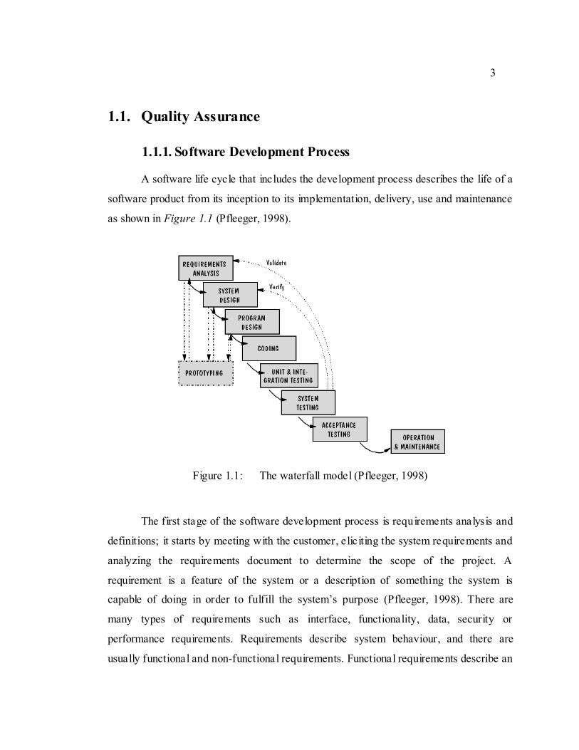
A software life cycle that includes the development process describes the life of a
software product from its inception to its implementation, delivery, use and maintenance
as shown in Figure 1.1 (Pfleeger, 1998).
Figure 1.1: The waterfall model (Pfleeger, 1998)
The first stage of the software development process is requirements analysis and
definitions; it starts by meeting with the customer, eliciting the system requirements and
analyzing the requirements document to determine the scope of the project. A
requirement is a feature of the system or a description of something the system is
capable of doing in order to fulfill the system‟s purpose (Pfleeger, 1998). There are
many types of requirements such as interface, functionality, data, security or
performance requirements. Requirements describe system behaviour, and there are
usually functional and non-functional requirements. Functional requirements describe an

4
interaction between the system and its environment, while non-functional requirements
or constraints describe a restriction on the system that limits our choices for constructing
a solution for the problem. Both types are elicited from the customer in a more or less
formal, careful way (Pfleeger, 1998). Even though requirements documents are done at
the first stage of the development cycle, they can be redefined and updated as the
development project progresses, with the consent of the client.
The next step in the software life cycle is to write a precise and detailed software
specifications document for the project, which is the system design. The specifications
document restates the requirements definition in technical terms appropriate for the
development of a system design; it is the technical counterpart to the requirements
definition document, and it is written by requirements analysts. Specifications can be
presented using different techniques such as use cases, data flow diagrams, event tables,
decision tables, UML flow charts, patterns, drawings, etc. There are also different types
of written specifications such as system or software requirements specificat ion, software
design specification, software test specification, software integration specification, etc.
The third step in a software life cycle involves the program design. It consists of
planning for a software solution, where software engineers develop a plan for a solution
for the project. The plan includes an architectural view of the software, low-level
components as well as any possible algorithm implementation issues.
At this point, the software requirements, specifications and design documentation
are done and thus in general the software is ready for the actual implementation stage.
One or more software engineers develop the code following the documentation.
The code will then be subject to a quality control procedure including validation
and testing, encapsulating the stages unit and integration testing, system testing and
acceptance testing. The quality control might include code inspection, formal method
validation and/or several types and levels of testing. An important quality assurance
activity is to present a plan to identify the types of validation and-or testing, the features
to be validated, the personnel and the schedule to do it (Software Testing Life Cycle,
2006).

5
At this stage, the software is ready for deployment on the client side and testing
of the installation. The cycle then extends to software maintenance as new discovered
problems might emerge and need to be fixed or new functionalities are required to be
added to the original system (Software Testing Life Cycle, 2006).
1.1.2. Quality Assurance Activities
In order to ensure the good quality of a product, quality assurance is all about
making sure that the project will be completed accordingly to the agreed upon
specifications, standards and functionalities required without any defects. For this
reason, quality assurance (referred to as QA) should be involved in the project from its
earlier stages. QA refers to the planned processes continuously monitoring the software
life cycle activities. It helps the teams communicating and understanding problems and
concerns, and plan, ahead of time, the testing environment required. It is mainly said to
be oriented to “prevention” (Quality Assurance and Software Testing, 2008).
In QA, records are kept concerning identified problems, which is an advantage
since steps can be taken in the future to avoid the same problems for the same or
different projects. This reduces significantly the total cost of a project as problems can
be eliminated in earlier stage, when the software is still under construction, and even
before the actual testing phase (Ruso, 2008).
Software verification and validation increase the reliability and dependability of
the product resulting also in decreased failure rates. It also decreases the maintenance
cost of the software that represents sometimes a large percentage of the total cost, due to
necessary corrective patches, software updates and service packs. In 2003, it was
reported that the relative cost for maintaining software and managing its evolution
represent more than 90% of its total cost (Seacord, Plakosh, & Lewis, 2003).
Another advantage of QA is an improved customer satisfaction. Because the
process of QA is designed to prevent defects, customers will be better satisfied with their
products leading to positive customer testimonials and thus a better company or product

6
reputation. In fact, the quality of the final software product can be a very decisive factor
in the market success or failure of a company.
QA activities start at the earlier stage of writing the requirements document. In
fact, most of the problems encountered in a software development are due to incomplete
requirements, lack of user involvement and unrealistic expectations (Pfleeger, 1998).
Thus, the first quality assurance process is to review the requirements document and
detect any possible problems, errors, inconsistency or ambiguity, anticipating and
deleting this way a large amount of possible software defects (Ruso, 2008). This QA
activity will also lead to success in accurately validating the resulting software to correct
user requirements.
Another QA main task is Process and Product Quality Assurance audits (PPQA),
which is an objective audit of each step of the software development to make sure it is
compliant with relative standards and process description. The QA team would
document any inconsistencies or problems and report it to the project staff (CMMI
Product Team, 2007). Audits are usually backed by standards as the ISO 9000 (a
standard that concerns quality systems that are assessed by outside auditors), CMMI (a
model of 5 levels of process maturity that determine effectiveness in delivering quality
software) or others.
QA activities include also monitoring the quality of the processes such as the
software design, the coding standards, code reviews, release management and any
change management that might be needed in the software platform. QA also
encompasses the quality control stage in the software life cycle. It consists of planning,
documenting and following the quality control outputs.
1.1.2.1. Quality Control
Quality control is a set of activities designed to evaluate the project output with
respect to its specifications. It starts after the code is done and it aims at proving that the
code is correct and error free. It is thus oriented to “detection” (Quality Assurance and
Software Testing, 2008). In general, quality control consists of verification, validation ,

7
and software testing; it includes activities such as walkthroughs, reviews, code and
document inspections, formal method verification, several types of testing, etc. It is the
responsibility of QA people to plan and document all these steps, to determine where the
interdependencies are and reduce the information into standard patterns for future use.
Software validation ensures that the final product has implemented all of the
requirements, so that each system function can be traced back to a particular requirement
in the specification (Pfleeger, 1998).
Software verification ensures that each function works correctly. Validation
makes sure the developer is building the right product and verification checks the quality
of the implementation (Pfleeger, 1998). Verification typically involves testing and code
evaluations through walkthroughs, inspections, checklists, etc. (Hower, 2009).
Testing is a process of executing a system with several input values with the
intent of finding errors and correcting them. In this master‟s thesis, we focus on software
testing as a mean for quality control, which is part of the quality assurance process. In
the following section, we will explain briefly what might cause failures in software, and
we will define some errors terminology. Then, we will discuss in details the different
types of software testing.
1.1.3. What Causes a Software Failure?
There are several possible causes for a software failure that we will discuss in
this section. But first we will define the used terminology for a better understanding of
the problem:
An error is committed by people, developers.
A fault is the result of such an error in software documentation, code, etc.
A failure in the system occurs when a fault is executed.
An incident is the consequence of a failure, but may or may not be visible to the
user.
A test case is an input and its expected software output.
Testing is executing test cases to find faults.

8
There are several possible reasons for software failures, the first one being a
miscommunication between customers and developers, especially in the presence of a
poorly elicited system requirements and specifications. In this case, the system is
delivered based on a wrong understanding of the requirements, thus generating lot of
failures from the user point of view.
Another possible reason for software failure is the software complexity. As the
complexity of current software applications increases, it becomes more difficult for non-
experienced developers to manage complex software development tools. Multi-tier
distributed systems, system applications utilizing multiple remote Web services,
enormous relational databases, security complexities, and large systems have all
contributed to the exponential growth in software/system complexity.
A third possible reason for software failure is of course development errors.
Programmers are humans and can make errors while coding. While some of these errors
are detected fast by the developer‟s test, some of them can stay hidden and require more
advanced testing techniques.
Another and very important possible cause can be the continuously changing
requirements or evolution of software. It is specially the case in poorly documented
software where, under time pressures, developers are required to do lot of guesswork
regarding an implemented feature when they are asked to modify, maintain, or add to it.
For this reason, QA is a key element to detect as much as possible of software errors
and prevent software failures. Companies that fail to implement QA standards and
adequately define the software testing plan for an application can destroy brand
credibility, sabotage the overall project, and create a cost blowout. We will discuss in the
next section the different testing strategies and types.
1.1.4. Software Testing
Software testing has traditionally been one of the main techniques contributing to
high software dependability and quality. It provides confidence in the system developed

9
and establishes the extent that the requirements have been met, i.e., what the users asked
for is what is delivered to them. Testing involves execution of a system under controlled
conditions and comparing the results with expected ones. The controlled conditions
should include both normal and abnormal conditions to determine any software failure
under non expected situations (Hower, 2009).
1.1.5. Testing Techniques
In a conventional program testing situation, a program P is executed on a set of
input values X and then the correctness of the output Y is examined. In the life cycle of
software though, there are several stages of testing, each having a different kind of input
values X and different goals or parts of P to test.
Figure 1.2: Testing activities (Pfleeger, 1998)
The testing stages illustrated in Figure 1.2 are:
Unit testing is the most „micro‟ scale of testing; it consists of testing functions or
code modules. It is based on module specifications and has complete visibility on
the code details.
Integration testing tests the modules or classes combined to determine if they
function correctly together. It is based on interface specifications representing how

10
a whole set of classes should interact together and thus it has visibility of the
integration structure.
System testing is based on the overall requirements of the whole system brought
together and it has no visibility of the code. It is based on the requirements and
functionalities of the system. It can be divided into two sub-testing types:
o The functional testing of the whole system to make sure the system
matches the system functional specifications.
o The performance testing of the software final measurable performance
characteristics.
Next, the system should be tested from a user perspective. Acceptation testing is
usually done by the customer or buyer of the system. It is based on the end-user
requirements to make sure the software answers the users‟ specifications and
requirements.
Finally installation testing is performed to test the software in the user‟s
environment. In some cases, an initial release of the software is provided to an
intended audience to secure a wider range of feedback. This is commonly calle d
beta testing.
Another kind of testing is the regression testing that consists of re-testing after
fixes or modifications of the software or its environment.
We can mainly divide testing strategies into two families: black box testing and
white box testing. The main difference between black box and white box testing is that
the underlying code of the software is used to determine the test-data in white box
testing. In contrast, in black-box testing, the test inputs and expected outputs are derived
solely from the functional specifications.
Black box testing is also known as functional, behavioural, opaque-box, or
closed-box testing; the tests done are based on the functional requirements of an
application and there is no visibility of the application code or internal structure. This
kind of testing is usually performed by a testing team different from the development

11
team. The types of testing under this strategy focus on testing functionalities of the
product. The base of the black box testing strategy lies in the selection of appropriate
data as per functionality and testing it against the functional specifications to check for
normal and abnormal behaviour of the system.
The testing stages usually done using the black box family techniques include
functional testing, system testing, user acceptance testing, sanity or smoke testing, beta
testing etc.
The main advantage of black box testing is that it allows checking the
conformance of the system with the specifications and thus it allows detecting missing
functionalities. It also scales up in the sense that it is used for different types of testing at
different granularity levels. However, the disadvantage of this strategy is that it depends
on the specifications and, thus, on the degree of details in the specifications. In other
words, poorly documented specifications can lead to poor functional testing. The other
weakness of black box is that it does not detect unexpected functionalities. If the system
performs unwanted behaviour for non specified input, the black box testing will not be
able to detect it because it selects test data based on the wanted behaviour in the
documentation.
The other testing strategy is white box testing. It is also known as structural,
glass-box, and clear-box testing. It is based on knowledge of the internal logic of the
code as well as its internal structure. Thus, tests are based on the code structure; there
are several white box coverage criteria:
Statement coverage: every statement in the code should be executed at least once,
since errors cannot be discovered if the parts containing them are not executed.
The problem with this criterion is that it doesn‟t ensure high dependability; for
instance it does not test the false outcome of an “if” statement with no else branch.
Branch coverage: all branches in the code are tested at least once. Branches are
basically parts of code under an “if”, “else”, “while”, “for” loops, etc.
Representing the code as a control flow graph, branch testing, or what is also
called edge testing, is generating test data to ensure each edge in the graph is

12
executed at least once. The problem is that while a certain input can make an “if”
true and thus traverse its branch, we will not be sure that this decision is 100%
correct. Other input might lead this decision to give unwanted result, and such
error will not be detected using this coverage.
Condition coverage: it is a strengthened branch testing. Each edge in a control
flow graph should be executed at least once, but also, if a decision is a compound
of several conditions, all possible values of the constituents conditions are
exercised at least once.
Modified Condition / Decision coverage: this criterion is in turn a strengthening of
the condition coverage. It consists of proving that every condition in a decision
affects the result of the decision in the desired way. Such criterion is able to prove
that a decision is correct and if an error exists, it is able to detect which part of the
decision generated the error. The focus of this Master‟s thesis is the automation of
this criterion that we will describe in details in the following sections.
The main advantage of white box testing is that it allows developers to be
confident about code coverage. It is also based on data and control flow and thus can
rigorously test every detail in the code. However, the main disadvantage of white box
testing is that it can miss cases omitted in the code; testing the code, developers cannot
detect required functionalities that were not included in the code.
In general, an understanding of the software lifecycle and the testing process in
the quality control stage is essential to any commercial software company.
Implementing best practice standards is part of the ongoing commitment of industry
professionals to the continual improvement paradigm. Still, no absolute certainty can be
gained from testing. Malicious errors can still go undetected. For this, testing should be
integrated with other verification activities, e.g., code inspection, formal verification ,
and other possible techniques.

13
1.2. Problem Definition
1.2.1. Automating Testing
While software testing is very important to make sure the developed software is
ready to be released on the market, testing can be very time consuming. It is reported
that 40 to 50% of software development effort is allocated for testing (Saha, 2008). A
survey done in 2002 by InformationWeek revealed that software testing consumes up to
50% of the total cost of the software development; this survey was followed by a second
one in 2002 in the province of Alberta, Canada, showing that only up to 30% of test
automation is done on the unit level, and the percentage drops even more for system and
integration level (Geras, Smith, & Miller, 2004).
There are several reasons why testing is time consuming. Let us consider an
application counting millions line of codes; the white box testing techniques alone
require lot of time to cover all the selected test criteria, which can cause a problem for
competing companies on the market. In fact, today, software managers and developers
are often asked to deliver complex software with ever-shrinking schedules and with
minimal resources. As a result, 90% of developers miss the deadlines and 91% are asked
to remove key functionalities late in the development cycle, allowing time to test the
functionalities already developed and release it on time. The reason is that often getting
a product to the market as early as possible can make the difference between the product
survival and death (Dustin, Rashka & Paul, 1999).
A solution to this problem is the automation of testing. Automating software
testing can be done mainly in two ways. The first way would be to create scripts with all
the required test cases embedded in them. This is extremely advantageous in the
regression testing, which consists of redoing all tests on the entire system after every
small change to make sure that the change didn‟t affect other working functionalities in
the system. In this case, it is extremely costly to redo manually the same tests over and
over again, when the scripts can be re-launched and the system is tested automatically. A
second advantage of automating testing with scripts is that it provides proof that the

14
tester did all the tests and no test was forgotten (Geras, Smith, & Miller, 2004). Another
advantage is the ability to run the scripts in parallel on different machines instead of
doing manual testing sequentially on one machine and thus to save lot of time, or even
let the scripts run all the tests all night long and report errors found without the need to
be supervised (Crestech Software Systems, 2008). Moreover, if the software is
environment-dependent, such as operating systems dependent, but has the same external
behaviour, then the tests should be performed on all the different possible environments,
which is of course very costly when done manually.
There are test automating tools in industry today that will create automated
scripts to test a system; the test cases should be provided to automate them. One
example is the TestComplete tool from Automated QA, promoted as “a tool designed to
free developers and QA departments from the massive drain on time and energy required
by manual testing”. The advantage is to run nightly scripts and collect the tests later
(AutomatedQA, 2009). Another example is the Test Plant tool that uses a scripting
language to automate the tests as well (TestPlant Ltd., 2008).
The second test automation method is to develop a tool that would automatically
generate test cases and run them on the application or system to be tested. Such a tool is
required to analyse the code under test, generate the test cases for a certain test criterion
and then generate the test data (Crestech Software Systems, 2008). Scripts can then
execute the application with the test data and check the output against expected results.
Such an automation tool is complex to develop and requires a software life cycle by
itself; however it can provide a huge time saving once it is done. In fact, since a program
is usually tested several times before it is released, the cost of writing the test suite is
sometimes regained before the program is even released (Volokh, 1990). More
importantly, an automation tool is usually done independently of the application or
system to test, and thus it can be used for different applications and systems. In other
words, the long life of an automation tool usually compensates its initial cost and results
in a big decrease in the software testing cost on the long run.

15
In general, automating test is easier to implement on white box testing
techniques than black box techniques. In white box techniques, the test cases to be
generated rely on the code itself, and thus it is possible to use code analysis techniques
to extract the necessary information needed to generate the test cases and the test data. In
most black box techniques, the test cases should be generated based on functionalities
written in natural language such as English or French. It is more difficult to create
techniques with the ability to analyse such languages and to extract the necessary
information required to generate the adequate test cases.
It is important to have automation tools engineered in an independent way of
the application to be tested. With the growing demand for rapidly developed and
deployed Web applications, we cannot afford to do and redo all the tests manually on the
applications, nor can we afford to reengineer automation frameworks for each and every
new application. Thus, it is an advantage to have a single tool for each test criterion that
will grow and continuously improve with each application and every diverse project that
challenges us; which is what we aim in this masters‟ thesis, developing an automation
tool for the MC/DC test criterion that would be applicable on Java programs; such a tool
does not exist in industry today.
1.2.2. Modified Condition/Decision Coverage Criterion
As stated above, avionic regulated domains should be compliant with the DO-
178B safety assessment document to get the approval of the Federal Avionic
Administration (FAA) for any software before its release in the avionic market. Because
of the importance and criticality of software in this domain, failures are non-affordable.
One testing criterion stated in the DO-178B document is the Modified
Condition/Decision Coverage criterion (MC/DC) for level A software. The document
divides the software into four levels, from level A to D, in a decreasing order of safety
criticality; level A being defined as “Where a software/hardware failure would cause
and-or contribute to a catastrophic failure of the aircraft flight control systems” by the
FAA (Hayhurts & al., 2001). No test automation tool exists currently for the MC/DC

16
criterion; for this reason we choose to develop such a tool for the test data generation for
MC/DC.
The goal of MC/DC testing is to make sure that each condition in a decision in
the application code affects correctly the outcome of this decision. This way, not only
the developers will test all the decisions in a code, but also every part of these decisions.
Later, we will describe in details how to generate test cases to cover this testing
criterion.
The MC/DC criterion is detailed in the report published by NASA, entitled “A
Practical Tutorial on Modified Condition/Decision Coverage” (Hayhurts & al., 2001),
but no implementation is provided. To the best of our knowledge, no automatic tool
exists today in the avionic industry (or other industries) that is able to automatically
generate test cases and test data for this criterion. This forms our main motivation to
develop a tool that would automatically test applications to cover the MC/DC criterion,
first by analysing the code under test, second by generating the appropriate test cases,
and third and most importantly by generating the appropriate test data for each test case.
For instance, if a program contains the decision “if (speed > 100 && force < 200)”, the
MC/DC criterion requires to prove that each part of the decision (speed > 100) and
(force < 200), called conditions, will affect correctly the outcome of this decision; i.e.,
the outcome of the decision is as expected. Thus, the MC/DC test cases to generate
would make the first condition (speed > 100) once true and once false while (force <
200) is fixed to true to show the effect of the first condition on the entire decision. The
same way, the second condition should be once true and once false while the first
condition is fixed to true. These test cases are generated automatically for the decision.
The next step would be to automatically generate the appropriate values of the variables
“speed” and “force” to satisfy the test cases, i.e., for the test case (speed > 100) false and
(force < 200) true, the tool should find a value for “speed” less than 100 and a value for
“force” less than 200.

17
1.2.3. Test Data Generation
Generating test data is a complex task. Let us consider that we want to test a
program that has two integer parameters x and y, and let us consider for now that we are
trying to generate the test data manually, the tester has usually a set of test cases to write
to cover the MC/DC or any other testing criterion. Covering a test criterion consists of
finding the appropriate test data, x and y, that would satisfy the criterion. If a test case
consists of making a condition in the middle of a code true, the tester can only
manipulate the parameters x and y of the program under test, and not any local variables
that might be used in the condition to be tested and their possible relationship with x and
y. Moreover, the admissible range for x and y in this case is the entire integer range, and
thus the tester has to guess the appropriate values for x and y from a 232
x232
possibilities.
As a result, searching for the test data manually can sometimes be impossible; an
automated code analysis technique is needed to extract the dependencies in the code and
then an automated search technique such as the meta-heuristic algorithms is needed to
search iteratively for the data in large search spaces.
In the following section, we summarize the activities required to attain the
MC/DC automation.
1.2.4. Extracting Code Dependencies
MC/DC criterion consists of testing every decision in the code. Thus we need to
locate the decisions in the code and extract their structure to generate the appropriate test
cases for them. We developed a parser to extract the decisions structure, as well as a
code instrumentation tool to trace the execution of the program for each test datum. A
third tool is needed to extract the dependencies in the code between the decisions.
Dependencies can be in two forms:
Control dependencies between nested decisions. In this case, if a decision is
nested into the true branch of an earlier decision, we say that the first decision
has control dependency on the second decision.

18
Data dependencies on the other hand are between the variables used in the
decision and prior variables in the code or with the program parameters.
Most suggested techniques for structural testing consider control dependencies , ignoring
data dependencies. This can cause a serious lack of guidance for the search in some
cases. On the other hand, a work done by McMinn in 2004 suggests data dependencies
as the appropriate tool to guide the search for data. This technique alone may lead to
incompleteness of guidance, and thus we worked to fully integrate both control and data
dependencies in the code analysis and be able to come up with an improved technique to
guide much more effectively the search for automatic test input data generation. As a
result, we propose a new and improved guidance function, also called fitness function,
for the generation of test cases and test data for the MC/DC criterion.
1.2.5. Meta-heuristic Algorithms
In today‟s literature, several works use meta-heuristic algorithms as search tools
to automate the data generation. Due to the computational complexity of the search
problem, exact techniques like linear programming are mostly impractical for large scale
software engineering problems and manual search is mostly impossible. Thus, Search-
based software engineering (SBSE) is an approach to apply meta-heuristic search
techniques like genetic algorithms, simulated annealing, and taboo search to seek
solutions for combinatorial problems at a reasonable computational cost. In SBSE, we
apply search techniques to search large search spaces, guided by a fitness function that
compare solutions with respect to the search goal and determine which is the better
solution and thus to direct the automated search into potentially promising areas of the
search space (McMinn, 2004).
For test data generation, this involves the transformation of test criteria to
objective functions. For each test criterion, a family of different objective functions is
needed. The algorithm iterates then to generate the appropriate data to make the fitness
function as close as possible to zero, meaning the algorithm found the data for the test
case.

19
1.2.6. Objectives and Contributions
SBSE are used in literature to automate the data generation for structural testing
such as statement testing and branch testing, however none explored the problem of
generating test input data for the MC/DC criterion. We use two meta-heuristics
algorithms, the genetic algorithm and the hill climbing algorithm, to automate the test
data generation, and we propose an improved cost function to better guide the search.
We test the automatic test and data generation on two benchmarks. We also use a
random generator that tries randomly selected data from the entire search space. The test
data generation is performed with the new cost function with integrated data
dependencies and with the traditional cost function relying solely on control
dependencies. Results show the superiority of the new fitness function. For the first
program, we are able to achieve 81% vs. 55% coverage with the genetic algorithm with
data dependencies and without respectively, 47% vs. 39% coverage with the hill
climbing and 40% coverage with the random (in this case nor data or control
dependencies influence the random generation of the data).
Overall, we are able to develop a testing automation tool that would first analyse
the code under test and collect all necessary information about control and data
dependencies of the code, second, generate a new improved fitness function for each
decision in the code, and third, use the fitness function as a guide to meta-heuristic
search algorithms to automate the test data generation for the MC/DC testing criterion.
We published our work at the 2009 Genetic and Evolutionary Computation
Conference. The article published is entitled ‘MC/DC Automatic Test Input Data
Generation’, by Zeina Awedikian, Kamel Ayari and Guiliano Antoniol.
20
Chapter 2: Related work
2.1. Search Based Search Engineering
Search Based Software Engineering (SBSE) applies search based optimization
algorithms to problems drawn from software engineering. The optimization algorithms
are used to identify optimal solutions and to yield insight. SBSE techniques can be used
for multiple objectives and-or constraints where the potential solution space is large and
complex (Harman, 2007). Such situations are common in software engineering, leading
to an increasing interest in SBSE.
The search based optimization algorithms used in SBSE are meta-heuristic
algorithms such as Genetic Algorithms, Hill climbing, Simulated Annealing , Random,
Taboo Search, Estimation of Distribution Algorithms, Particle Swarm Optimization, Ant
Colonies, LP, Genetic programming, Greedy algorithms. The search mechanism of
these algorithms in large search spaces is guided by a fitness function that captures
properties of the acceptable software artefacts we seek.
In the past five years, SBSE techniques were used for several applications such
as Regression testing (Li, Harman, & Hierons, 2007), model checking (Ferreira &al.
2008), maintenance (Antoniol, Di Pentan & Harman, 2007), test generation (McMinn &
Holcombe, 2006), etc. We are mostly interested in the application of SBSE to software
testing.
2.1.1. Search Based Software Testing
We use the term Search Based Software Testing (SBST) throughout our work to
indicate the application of SBSE to the testing problem. A major issue in software
testing is the automatic generation of the testing inputs to be applied to the program
under test.
21
To cover a test criterion, a set of test cases should be met. For each test case, the
parameters of the application or the system under test should be generated in a specific
way to satisfy the test case, which is called test data generation. One way to generate the
data is to explore the entire parameter‟s space in order to find the appropriate
combination of values. However, for applications with several parameters, exploring the
entire parameter‟s space can increase exponentially, and an exhaustive search becomes
impossible. For instance, aerospatiale applications can take up to 10 or more parameters;
in such cases, if the parameters are integers, the parameter‟s space is 2(10*32
). A solution
to this problem is to use a heuristic technique which is use an approximation algorithm
to search for the data. Such a technique risk to either not find a solution, when there
exists one, or to find a non optimal solution. However, it allows searching for the data in
a reduced search space and in a reduced search time.
A number of approaches based on heuristic search methods have been
developed; in general SBST uses search based optimization techniques to formulate the
test data generation problem as a search problem (Lakhotia, Harman, & McMinn, 2008).
This problem is then addressed using search methods; it can also be formulated as a
constraint optimisation problem or a constraint satisfaction problem (Sagarna & Yao,
2008).
The meta-heuristic search techniques used in SBST are high-level frameworks
that use heuristics to find solutions to combinatorial problems at a reasonable
computational cost. Since meta-heuristic algorithms need a fitness function representing
the combinatorial problem to guide the search; the testing criterion is transformed into
the fitness function. The search space is the space of possible inputs to the program
under test.
SBST has proved to be effective partly because it has a wealth of optimization
techniques upon which to draw and because the generic nature of the approach allows it
to be adapted to a wide range of test data generation problems; in principle, all that is
required to adapt a search based technique to a different test adequacy criterion is a new
fitness function (Lakhotia, Harman, & McMinn, 2008).

22
Works on search based approaches to software engineering testing problems date
back to as early as 1976, when Miller and Spooner used optimisation techniques for test
data generation (Miller & Spooner, 1976). In 1992, Xanthakis et al. were the first to
apply meta-heuristic optimization search for test data generation (Xanthakis et al. ,
1992). In recent years, several approaches that use meta-heuristic search techniques to
automatically obtain the test inputs for a given test criterion have been proposed. We are
mainly interested in works done on structural testing since the MC/DC is a structural
testing criterion.
In the following section, we present two main works done in this field, the first
one is by Miller and Spooner, as it was the first work to use search based optimisation
techniques for test data generation (Miller & Spooner, 1976). The second work done by
Korel is the first to use data analysis to help the heuristic search (Korel, 1990). In the
next section entitled Meta-heuristic search algorithms, we will present more recent work
that use different search approaches for SBST problems.
2.1.2. Structural Testing
Automation of structural coverage criteria and structural testing has been the
most widely investigated subjects. The first strategy used to automate the test data
generation for structural testing is a local search used by Miller and Spooner back in
1976 (Miller & Spooner, 1976). Their goal was to automate the generation of input data
to cover particular paths in a program. They formulated the problem as a numerical
maximization problem and they used a “heuristic” approach to solve it. However, they
were only interested in generating floating point data to cover the test cases of the
branch testing criterion. The used approach fixes any integer parameters in the program,
and tries to generate values for the remaining floating point parameters for each possible
path in the program. Since each program execution takes the form of a straight line
program, it is possible to collect any path constraints for a given execution. The
collected constraints form the search fitness function. Then, starting from an initial
random point, the approach applies numerical techniques for constraint maximization.
The search iterates until the fitness function become positive. Since the goal here is to

23
make the fitness function positive, and any point with positive fitness is equivalent, there
was no need to consider the cases of local optima (Miller & Spooner, 1976).
This approach has two drawbacks. First it only targets floating points parameters;
second, often infeasible paths are selected; as a result, significant computational effort is
wasted analyzing these paths and trying to find data covering them.
This work was later extended by Korel in 1990 (Korel, 1990). While the first
work relies on the static constraints in the program execution to form the fitness function
guiding the search, Korel uses a dynamic technique that relies on the actual execution of
the program with input data. The goal is again to cover the branch testing criterion.
Initially the program is executed with arbitrary input. During each execution for a
targeted branch, a search procedure determines whether the execution should continue
through the current branch or an alternative branch should be taken. This decision is
made based on the control flow graph of the program, determined prior to the execution
of the program. Branches are classified into categories, critical branches, required
branches, semi-required branches, and non-required branches. These categories
represent the control dependencies between branches. Thus, if the execution flow is
diverging from the targeted branch, a real valued function is associated with this branch;
the fitness value. A minimisation search algorithm is then used to automatically generate
data to change the flow of execution at this branch. In order to speed up the search,
Korel uses a data flow analysis technique to determine input variables that are
responsible for the undesirable program behaviour. The technique is used for programs
with a high number of parameters such as big size arrays, and it aims at detecting which
of the input influences more the targeted branch. Thus, if T=<nkl,nk2,...,n > is a path
traversed on a program input x, where x can be an array of 30 elements, the technique
determines the influence of the elements of x on the nodes in the path in terms of used
variables, and the influence of each node nk on the node following it until the targeted
branch is reached. This way, for a certain target branch, the author only considers the
influential input variables (elements of the array in our example) in the search procedure
(Korel, 1990).

24
Though this approach presents improvements on the previous work (Miller &
Spooner, 1976), it does not present an implementation of the data flow analysis. On the
other hand, the data flow analysis is used only to select the input variables influencing
the branch to test and thus starting the search of required data for these variables.
However, the author does not take advantage of dependencies to actually guide the
search using the data flow analysis information. This is what we call data dependencies
between the nodes of the program, and it can actually help the search converge faster to
the required solution.
The local search used to find the test data can lead to local optimum solutions in
the search space when trying to minimize the fitness function. In order to overcome this
problem, researchers investigated more sophisticated search techniques such as the
simulated annealing, hill climbing, and evolutionary search algorithms. We will discuss
the work done on these algorithms in the following section.
2.2. Meta-heuristic Used To Automate Test Data
Generation
For each problem solved using meta-heuristic techniques, there are usually two
main decisions of implementation. The first one being the encoding of the solution, i.e.,
the structure (e.g., array, tree), how many variables it has, their types, etc, and the second
main decision is the transformation of the test criteria into a fitness function. The fitness
function, models the closeness of the input data to cover the criterion tested. It is usually
calculated at the end of each algorithm iteration and it compares and contrasts the
solutions with respect to the overall search goal to guide the search into a promising
neighbourhood of the search space.
There are several types of meta-heuristic algorithms that were used in literature to
automate the data generation. We will describe here works based on the simulated
annealing algorithm and the evolutionary techniques, such as the genetic algorithm.

25
2.2.1. Simulated Annealing
To overcome the limitations associated with local search optimum, Simulated
Annealing (SA) was used as another type of meta-heuristic search algorithms. Tracey et
al. proposed in 1998 an optimisation-based framework to be applied to a number of
structural testing problems (Tracey et al., 1998). Tracey‟s work focuses on branch
coverage. Their goal is to search for program input which forces execution of the desired
part of the software under test. For the search to succeed, a fitness function is needed to
guide the search, relating a program input to a measure of how “good” the input is to
achieve a certain test target. The fitness function returns good values for test-data that
nearly executes the desired statement and bad values for test-data that is a long way from
executing the desired statement. In general, the input domain of most programs is likely
to be very large, and given the complexities of systems it is extremely unlikely that the
fitness surface would be linear or continuous. The size and complexity of the search
space therefore limits the effectiveness of simple gradient-descent or neighbourhood
searches as they are likely to get stuck in locally optimal solutions and hence fail to find
the desired test-data (Tracey et al., 1998). Thus a more sophisticated approach is needed
such as the SA. SA allows movements which worsen the value of the fitness function
based on a control parameter known as the temperature. At the early stage of the search
iterations, inferior solutions are accepted with relative freedom, but as the search
progresses, accepting inferior solutions becomes more and more restricted. The aim of
accepting these inferior solutions is to accept a short term penalty in the hope of longer
term rewards.
The fitness function designed by Tracey et al. evaluates to zero if the branch
predicate evaluates to the desired condition and positive otherwise. It is designed based
on the structure of the system under test; for each predicate controlling the target node, if
the target node is only reachable if the branch predicate is true then the fitness of the
branch predicate is added to the overall fitness for the current test-data otherwise the
fitness of ¬(branch predicate) is used. For loop predicates, the desired number of
iterations determines whether the fitness of the loop predicate or ¬(loop predicate) is
26
used. The simulated annealing search uses this to guide its generation of test-data until
either it has successfully found test-data or until the search freezes and no further
progress can be made (Tracey et al., 1998).
The automation framework was tested on small Ada 95 programs to cover the
branch coverage criterion. The programs ranged from 20 to 200 lines of codes. The
reported coverage percentage is 100% for all but one case; the failing case achieved
100% branch coverage in 40 out of the 50 trials. The search time of SA is 2 to 35
seconds. Unfortunately, the programs tested are not available and thus we were unable to
verify their structural complexity. Moreover, no comparison with other search
techniques performance is presented. Still, this work provides an automated platform for
structural testing. We aim in our work to build a similar platform, however achieving the
MC/DC coverage and not the branch coverage.
2.2.2. Genetic Algorithm
Evolutionary approaches are search algorithms tailored to automate and support
testing activities, i.e., to generate test input data. They are often referred to as
evolutionary based software testing or simply Evolutionary Testing (ET). Genetic
algorithm (GA) is an ET algorithm.
2.2.2.1. Real Time Testing
In 1997, GA was used by Wegener & al. to test real-time systems for functional
correctness. A common definition of a real-time system is that it must deliver the result
within a specified time interval and this adds an extra constraint to the validation of such
systems, namely that their temporal correctness must be checked (Wegener, Sthamer,
Jones, & Eyres, 1997). The standard technique for real-time testing is the classification-
tree method; it was used to generate the test cases forming the objective of the search.
The genetic algorithm aimed to find the longest execution time, and then the shortest of
the real system response time. Wegener et al. concluded from their work that genetic
algorithms are able to check large programs and they show considerable promise in

27
establishing the validity of the temporal behaviour of real-time software (Wegener,
Sthamer, Jones, & Eyres, 1997).
Figure 2.1: Block diagram of the genetic algorithm (Wegener & al., 1997)
The used GA‟s block diagram is illustrated in Figure 2.1; the algorithm iterates
with a population of candidate solutions. It initialises with a randomly generated
population then it evolves by combining and mutating the current generation in order to
generate possible solutions. An evaluation is performed on the newly generated
solutions and a selection technique is then used to transmit only the fittest individuals
into the next generation. The algorithm iterates until a solution is found to satisfy the
optimisation criteria.
2.2.2.2. Data Flow Testing
A recent work by Ghiduk et al. in 2007 applies GA to search for test data to
satisfy the data-flow coverage criteria; which is a structural criterion, by generating a
test suite to cover the all-uses coverage criterion. Data flow analysis determines the
definitions of every variable (statement where the variable is defined) in the program
and the uses (statement where the variable value is used) that might be affected by these

28
definitions. Thus, the all-uses criterion consists of generating a set of test cases T, such
that for every variable v in the program, T contains at least one definition clear path
from every definition of v to every reachable use of v. The genetic algorithm used is fed
with one test goal t T at a time and generates the test data satisfying this test goal. To
generate the appropriate fitness function for each test goal, the technique uses the control
flow graph of the code under test. The control flow graph is mostly used to detect the
nodes where variables are defined and used, and then the genetic algorithm tries to find
input data to cover the pairs of (definition, use) for each variable v. The program under
test is executed for each test data and the path of the execution is recorded. The path is
then used to calculate the closeness of the input data to the clear path sought; a clear path
being a path with no modification applied on the variable between its definition and its
use. In the search process, parameters are encoded into binary values and the crossover
and mutation is applied on binary values. The resulted individuals are decoded back into
the real parameters types (Ghiduk, Harrold, & Girgis, 2007).
The technique was tested on nine programs ranging between 20 and 60 lines of
code, and between 11 and 88 def-use pairs. The results of the work can be summed as
follows:
On average the genetic algorithm needs 79 seconds, 628.56 iterations, and
4112.56 test cases to satisfy 93.25% of the test requirements of all programs to
cover all-uses criterion
A random search technique needs 180.22 seconds, 1251.56 iterations, and
6879.11 test cases to satisfy 79.81% of the test requirements of all programs.
The results show the superiority of the GA search. However, two important threats to
validity can be summarized as follows, first, the programs tested are small and do not
represent a random selection over the population of programs as a whole. The second
threat to validity is that results are compared to a random data generator that is usually
not sufficient to evaluate the reliability of the technique (Ghiduk, Harrold, & Girgis,
2007).

29
2.2.2.3. Class Testing
A recent contribution by Tonella in 2004 has demonstrated ET applicability to
the problem of object-oriented testing, more precisely to unit testing of classes. Unit
testing is a white box technique that considers one class at a time, executing the class
with different input values and verifying the expected results. The class is isolated from
the rest of the software and required classes are made available using stubs. The
complexity of class testing in an object oriented environment is caused by the object
state, the many possible usage scenarios of an object and the large search space.
Figure 2.2: Automation of test cases generation using ET (Tonella, 2004)
In Tonella‟s approach, the functionalities of classes are tested first by testing the
total outcome of the methods, then code coverage is targeted, using structural coverage,
and data flow coverage. Thus, the fitness function is build based on the state of the
objects in a class, each object‟s parameter, action and value, as well as each method
signature, call and parameter contribute to form a chromosome reprensenting the fitness

30
function. ET is then used to automate the test case generation. The mutation used in the
genetic algorithm is a one-point mutation, where either a parameter value is changed, or
a method signature, or a method call insertion, etc (Tonella, 2004).
The algorithm was tested on seven classes taken from the java.util library with
the number of line of codes ranging from 100 to 1,000 approximately and having
between 6 and 26 public methods. Artificial errors were inserted in the classes. The
results showed an average test coverage of 95% and the tests were able to find an
average of 77% of the inserted errors. The method was able to find powerful and
compact test suites, however it was not fully automated. It needed manual tweaking and
annotation, and no oracle was available to use as a comparison tool (Tonella, 2004).
2.3. Search Fitness Function
2.3.1. Traditional Fitness Function
ET has proved its effectiveness in searching for test data (Wegener, Baresel, &
Sthamer, 2001). In most evolutionary approaches for structural testing, the traditional
fitness function is composed of two components:
f(x) = approach level + branch distance
The first component accounts for control dependencies and it is often referred to
as the approach level, or approximation level. It measures how close in structural terms
the input is from reaching the target. Thus, it is usually the count of critical nodes in the
control flow graph between the target and the node where the execution diverged
(Baresel, Sthamer, & Schmidt, 2002).
For example, Figure 2.3 presents a simple code for the Calc method. The
statement at line 17 depends on the ‟if‟ statements at lines 12, 13 and 16: the ‟if‟
statements at lines 12, 13 and 16 control the execution of line 17. Control flow nodes in
the program Control Flow Graph (CFG) corresponding to those ‟if‟ statements are called
the critical branches because they can cause the flow to diverge to unwanted code
regions. The approach level for a test input datum is computed by subtracting one from
the distance in critical branches. Going back to the target line 17, if the flow diverges at

31
line 13 (two control nodes in between), the approach level assign a fitness value of one.
Thus, approach level measures how close we are to line 16 “if”, the last controlling
statement (McMinn, 2004).
Figure 2.3: Example of code under test
The second component of the fitness function is the branch distance. It is
computed either at the branch where the input diverged (Baresel, Sthamer, & Schmidt,
2002), or at the target node if the input x did not achieve the test case at this node. It is
used to overcome the limitation of the first fitness component; if the search generates
input data leading to the target without satisfying the test case at the target, all critical
branches are satisfied and thus the approach level fitness is zero, also if two input values
diverge at the same critical node, the approach level is the same for both of them. In
these two cases, the approach level is no longer effective in guiding the search and the
branch distance is needed. The later calculates how close the input is from satisfying
either the target or the branch where it diverged (McMinn, 2004). A work presented by

32
Bottaci in 2003 explores how to calculate effective branch distance functions (Bottacci,
2003).
This fitness function has a limitation when the code under test contains flag
conditions or data dependencies between the variables of the code. In this case, the
fitness function fails to guide the search, leading to a random search. We will discuss
this issue in details in the next two sections.
2.3.2. Fitness Function For Flag Conditions
In 2005, Liu and al. addressed the problem of flag conditions in the code under
test. While ET proved its effectiveness in automatically generating test data, the
presence of flag variables makes the search degenerates into a random search for
structural testing. The problem in such techniques is that they rely on a fitness function
solely derived from the control dependencies between nodes based on the control flow
graph. When the target statement is controlled by an “if” containing flags and these
having data dependencies from prior statements not contained in the control
dependencies predicates of the target, the fitness function is no more effective in guiding
the search.
Figure 2.4: A simple example of flag conditions (Liu et al. , 2005)
For example a flag variable use is illustrated in Figure 2.4 at line 10. While the
“if” at line 10 contains the “flag” variable, and the value of “flag” depends on its
modification in prior statement, there is no mean to make its value true based on the
control dependencies that the “if” has (in this example it has none).
33
In general, flag variables only hold two values, either true or false; thus the
fitness function can no more differentiate the degree of closeness and the fitness
landscape becomes plateaux (Liu, Liu, Wang, Chen, & Cai, 2005). Liu and al. presented
a new fitness function composed of two parts, the f irst is the same approach level and
the second is flag cost function related to the flag definition statements. Since the flag
value is defined by its definition statements (example flag = true at line 9 in Figure 2.4),
it is required to consider the data dependence relationship between the use of the flag
and its definitions, to calculate the branch distance. Each flag has a definition set
Df=<d1,d2,...,dm>, where each node in this set is a definit ion statement of the flag. Also,
each feasible path to the target has a conditional statement set C f=<C1,C2,...,Cm>. When
Ci is true, an assignment statement of f will be executed, whereas, when Ci is false, the
assignment statement fails to be executed. Generally, at the ith
conditional statement Ci ,
if branch di assigns true to the flag, the condition Si which keeps the flag true at Ci+1 is
Si−1 ∨ Ci. For example, in Figure 2.4, in order to make flag true at the conditional
statement of line 10, S(1) = x > 4, S(2) = S(1) ∧ ¬ (x= =2), S(3) = S(2) ∨ (y > 6) (Liu,
Liu, Wang, Chen, & Cai, 2005).
An empirical study was conducted on different programs with flag. The approach
uses a genetic algorithm with a population size of 49, crossover probability of 0.2 and
mutation probability of 0.02. The algorithm stops when the test data are found or after
10,000 iterations. The algorithm runs using the traditional fitness function, then using
the new fitness function. Also, the authors compare their approach to the flag avoid
approach that we will present next. In the later approach, the code under test is modified
in a way to avoid the flag use. For example, the code: if (a == 0) {flag = true} is
replaced by: flag = (a[i] == 0). The results show a tremendous decrease in the number of
fitness evaluations with the use of the new fitness function, Figure 2.5 sums the results.

34
Figure 2.5: Results of flag problem approach (Liu et al., 2005)
Even though this approach presents a large improvement in the data generation
for code with flag problems, it is specialized to flags and does not scale to the problem
of data dependency between any types of critical nodes. For instance, a local variable
can be modified several times in a code and then used in a predicate (for example at line
8 of Figure 6 instead of y>6), the traditional fitness function leads to a random search,
because the new fitness function proposed by Liu does not apply the data dependence
analysis on non flags variables.
Another approach to solve the flag problem is the flag avoid approach that
transforms code with flags into flag free codes (Harman, Hu, Hierons, Baresel, &
Sthamer, 2002). The purpose of this approach is to also overcome the problem of
flattened fitness landscape. Evolutionary testing is used to generate test data to cover
certain structural criteria. An example of a transformation is illustrated in Figure 2.6.

35
Figure 2.6: Flag removal example (Harman et al. , 2002)
Column (d) is equivalent to the original code in column (a) but easier to test
because the flag is replaced by an expression that denotes its value at the point of use.
Columns (b) and (c) are intermediate transformation steps introducing a temporary
variable to capture the value of the variable “n”. The approach also treats the cases
where there is no clear definition path between the flag definition and its use in the
condition as illustrated in Figure 2.7.
Figure 2.7: Flag removal example 2 (Harman et al., 2002)
Results were presented for experiments conducted on two flag-based programs to
generate test data before and after the transformation, the Triangle program used as
benchmark in our work as well, and a Calendar program. For the Triangle program,
40,000 fitness evaluations were not able to attain coverage of 86%, w here 25,000 fitness
evaluations were enough to attain the 86% on the transformed code. Also the maximum
coverage is attained only on the flag-free code. For the Calendar program as well, the
maximum achieved coverage is attained on the transformed program.
This work was extended in 2007 to cover the issue of function-assigned flags
(Wappler, Baresel, & Wegener, 2007). A new approach is used, injecting a distance
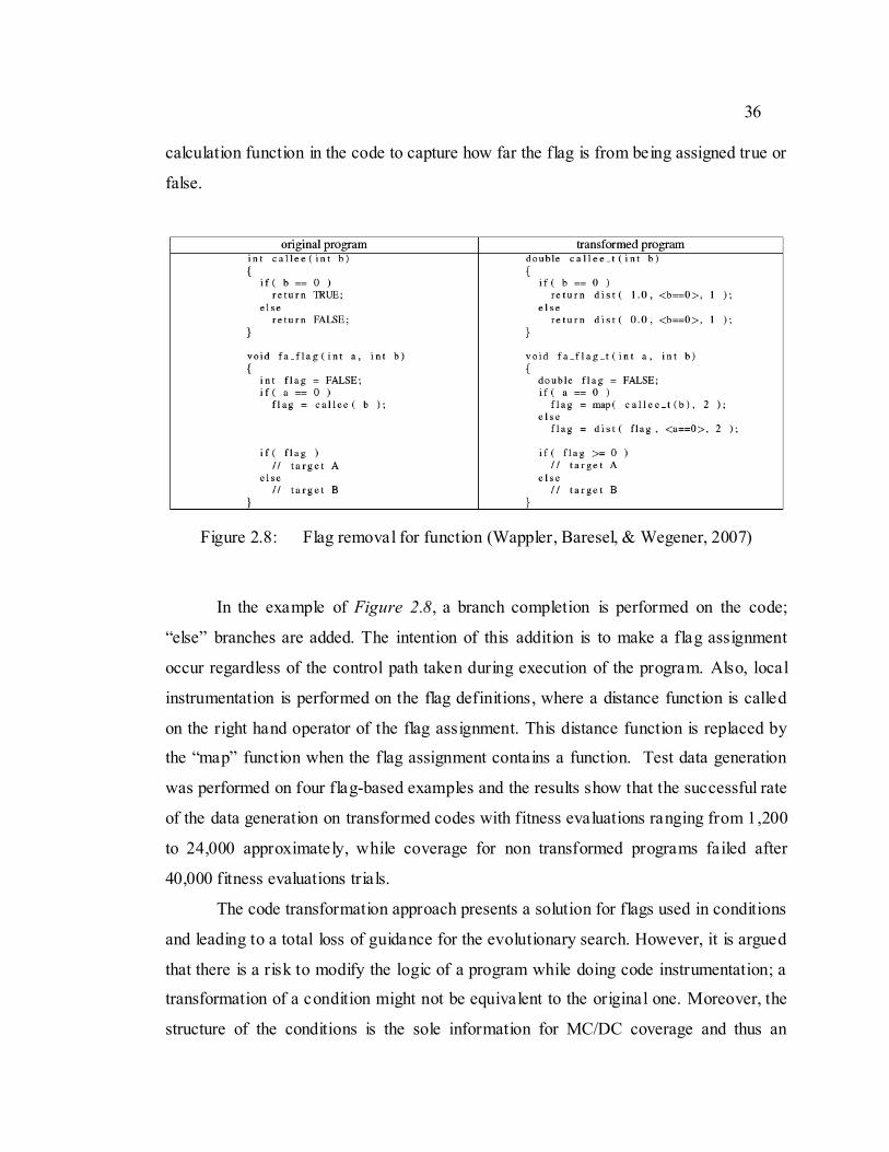
36
calculation function in the code to capture how far the flag is from being assigned true or
false.
Figure 2.8: Flag removal for function (Wappler, Baresel, & Wegener, 2007)
In the example of Figure 2.8, a branch completion is performed on the code;
“else” branches are added. The intention of this addition is to make a flag assignment
occur regardless of the control path taken during execution of the program. Also, local
instrumentation is performed on the flag definitions, where a distance function is called
on the right hand operator of the flag assignment. This distance function is replaced by
the “map” function when the flag assignment contains a function. Test data generation
was performed on four flag-based examples and the results show that the successful rate
of the data generation on transformed codes with fitness evaluations ranging from 1,200
to 24,000 approximately, while coverage for non transformed programs failed after
40,000 fitness evaluations trials.
The code transformation approach presents a solution for flags used in conditions
and leading to a total loss of guidance for the evolutionary search. However, it is argued
that there is a risk to modify the logic of a program while doing code instrumentation; a
transformation of a condition might not be equivalent to the original one. Moreover, the
structure of the conditions is the sole information for MC/DC coverage and thus an

37
approach relying on the transformation of the conditions to logically equivalent ones but
structurally different cannot be used for MC/DC. The generated test cases would not
satisfy the coverage criterion.
2.3.3. Chaining Approach Integrating Data Dependencies
As stated above, the search algorithms can degrade to a random search due to a
lack of guidance to the required test goal. Often this happens because the traditional
fitness function does not take into account data dependencies within the program under
test, and because certain program statements need to have been executed first in order to
reach the target statement (McMinn & Holcombe, 2006).
Figure 2.9: Code with one problem node (McMinn & Holcombe, 2006)
Figure 2.9 is an example of a code where the target in line 7 relies on a flag
variable “flag” that was modified in prior statements. The traditional fitness function,
relying solely on the control dependencies of predicate at line 6, fails to guide the search
as the predicate has no control dependencies.
To overcome this problem, McMinn proposed in 2004 and 2006 to integrate data
dependencies in test data generation to improve the search process, extending the
chaining approach of Korel (Korel, 1990). If the search fails to find test data that directly
executes the target, the Chaining Approach performs data flow analysis to identify

38
intermediate statements that may determine whether the target will be reached or not.
By incorporating data dependencies into ET, the evolutionary search can be directed into
potentially unexplored, yet promising areas of the test object‟s input domain (McMinn &
Holcombe, 2006).
In the chaining approach, an event sequence is a sequence of events, < e1, e2, ...
ek >, where each event is a tuple ei = (ni, Ci) where ni is a program node and Ci is a set of
variables referred to as a constraint set (Ferguson and Korel, 1996). The constraint set is
a set of variables that must not be modified until the next event in the sequence. That is
to say, a definition-clear path must be executed between two events e i and ei+1 with
respect to each variable v in Ci.
McMinn defines a problem node as a branching node for which the search cannot
find inputs. The set of nodes that can have an immediate effect on a problem node is the
set of last definitions of variables used at that problem node. A last definition i is a
program node that assigns a value to a variable v which may potentially be used by a
node j. For the node to qualify as a last definition, a definition-clear path must exist
between node i and node j with respect to v. In the example of Figure 2.9, the path < 4, 6
> is definition-clear with respect to the variable flag, but < 4, 5, 6 > is not, bacause flag
is defined at node 5.
The Chaining Approach first introduced by Korel begins with an initial sequence
E0 = < (s, φ), (t, φ) > that contains the start node s and the target node. Both events have
empty constraint sets. The test data search may fail to find inputs to execute the event
sequence, with the flow of execution diverging down an unintended branch at some
node p1. In our example, input data may not be found to take the true branch from node
6 so that node 7 is executed, due to the existence of a flag variable in the predicate at
node 6. Therefore, node 6 is declared as a problem node. Node p1 (node 6) is then
inserted into the event sequence: < (s, φ), (p1, φ), (t, φ) >. For the problem node p1, the
set of last definition nodes lastdef(p1) are found for the set of variables used at p1. For
each last definition di ϵ lastdef(p1), a new event sequence is generated containing an
event associated with that last definition:
E1 = < (s, φ), (d1, {def(d1)}), (p1, φ), (t, φ) >

39
E2 = < (s, φ), (d2, {def(d2)}), (p1, φ), (t, φ) >
. . .
EN = < (s, φ), (dN, {def(dN)}), (p1, φ), (t, φ) >
The addition of the last definition variable into the constraint set specifies that it
will not be modified again until the problem node is encountered; ensuring the effect of
that last definition on the problem node is not destroyed (Korel, 1990).
In Figure 2.9, the last definition nodes for node 6 are identified as nodes 1, 3 and 5
and the three new generated event sequences are:
E1 = < (s, φ), (1, {flag}), (6, φ), (7, φ) >
E2 = < (s, φ), (3, {flag}), (6, φ), (7, φ) >
E3 = < (s, φ), (5, {flag}), (6, φ), (7, φ) >.
The constraint set contains the variable “flag”. In event sequence E1, this means
that the false branch must be taken from nodes 2 and 4 to prevent flag being redefined
before node 6. E2 requires flag to be set to true at node 3. This requires node 2 to be
executed as true and so the search can use the branch distance information at this node to
find a value of “a” for this to happen. This branch distance information explicitly directs
the search to the zero value of the “a” variable. Such guidance was not available from
the branching condition at node 6, which depends only on the flag variable (McMinn &
Holcombe, 2006).
The Chaining Approach selects one of the event sequences and tries to find
inputs for which it is successfully executed. If such an input is found, then test data to
execute the test goal has been found. If not, new event sequences need to be generated.
In the original approach proposed by Korel, the new sequences are generated based on
the same problem node, tracing back in the last definitions of this node. This approach
then has limitations when more than one problem node is encountered in a feasible path,
i.e., when the last definition of the current problem node depends on the use of another
problem node. To overcome this limitation, McMinn extended the chaining approach to
generate new event sequences based on newly found problem nodes.

40
Figure 2.10: Code with multiple problem nodes (McMinn & Holcombe, 2006)
Based on the initial chaining approach, the event sequences generated are:
E1 = < (s, φ), (3, {shutdown}), (9, φ), (10, φ) >
E2 = < (s, φ), (8, {shutdown}), (9, φ), (10, φ) >
E1 is infeasible, E2 on the other hand is feasible, but node 9 remains problematic,
because it requires node 8 to be executed. This node is always executed, but no new
information is added to the fitness function, whose landscape is still flat. To handle this
problem, an extension is made to the event sequence generation algorithm, using the
concept of influencing sets. An influencing set consists of all variables that could
potentially affect the outcome at the problem node. Thus, the event sequence generation
process is forced to consider definitions for all variables that can potentially affect the
problem node. For a newly identified problem node, the influencing set is simply the set
of variables involved in evaluated, but unsatisfied conditions, at the problem node.
Beginning with the current problem node sn, the initial influencing set I, and the event
prior to the problem node event in the event sequence e = (n, C), the algorithm traces its
way backwards through the nodes of the program. Returning to E2 =< (s, φ), (8,
{shutdown}), (9, φ), (10, φ) >, node 9 is still problematic. In event sequence generation,
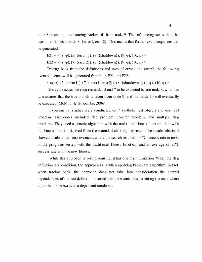
41
node 8 is encountered tracing backwards from node 9. The influencing set is then the
uses of variables at node 8: {error1, error2}. This means that further event sequences can
be generated:
E21 = < (s, φ), (5, {error1}), (8, {shutdown}), (9, φ), (10, φ) >
E22 = < (s, φ), (7, {error2}), (8, {shutdown}), (9, φ), (10, φ) >
Tracing back from the definitions and uses of error1 and error2, the following
event sequence will be generated from both E21 and E22:
< (s, φ), (5, {error1}), (7, {error1, error2}), (8, {shutdown}), (9, φ), (10, φ) >
This event sequence requires nodes 5 and 7 to be executed before node 8, which in
turn assures that the true branch is taken from node 9, and that node 10 will eventually
be executed (McMinn & Holcombe, 2006).
Experimental studies were conducted on 7 synthetic test objects and one real
program. The codes included flag problem, counter problem, and multiple flag
problems. They used a genetic algorithm with the traditional fitness function, then with
the fitness function derived from the extended chaining approach. The results obtained
showed a substantial improvement, where the search resulted in 0% success rate in most
of the programs tested with the traditional fitness function, and an average of 95%
success rate with the new fitness.
While this approach is very promising, it has one main limitation. When the flag
definition is a condition, the approach fails when applying backward algorithm. In fact,
when tracing back, the approach does not take into consideration the control
dependencies of the last definition inserted into the events, thus omitting the case where
a problem node exists in a dependent condition.

42
Figure 2.11: Calc method with data and control dependencies needed
In Figure 2.11, following the extended chain approach, “result” data
dependencies is included in the fitness evaluation. However, “result” definition at Calc
line 10 is controlled by the “if” at line 8; much in the same way, “Fail” definitions (lines
5 and line 7) are controlled by the “if” at line 4. Because the approach does not take into
consideration the control dependencies of the last definitions of the problem nodes,
control node 8 and 4 are not considered in the event sequences. As a result, we have a
lack of information regarding how to make the flag “Fail” false and the whole
evolutionary search will stagnate and degrades again into a random search.
For this reason, in our work, we will extend the chaining approach to incorporate
control nodes such as nodes 8 and 4 into the approach level fitness.
The second disadvantage of McMinn‟s approach is the high number of fitness
evaluations needed to achieve the test coverage. The example codes tested required a
minimum of 55,000 and a maximum of 300,000 fitness evaluations because the
approach works sequentially; it starts with one event sequence, and if test data is not
found, a new event sequence is generated and the search starts all over. To overcome
this time consuming drawback, we propose to generate all possible data dependencies
sequences, and run them in parallel, each in its own execution thread.
43
Chapter 3: SBST and Meta-heuristic algorithms
We present in this chapter the general concepts in Search Based Software
Testing. Detailed implementation will be explained in next chapters.
3.1. Search Based Software Testing
Search based software engineering (SBSE) aims at solving software problems by
applying search techniques to explore large search spaces, guided by a fitness function
that captures properties of the acceptable software artefacts we seek.
We are mostly interested in the application of SBSE in testing, more precisely
the automation of test data generation. The generation of input data can be modeled as a
search problem in a large search space that we aim to optimize. Thus, we can easily
apply the SBSE techniques to our problem. We use the term Search Based Software
Testing (SBST) throughout our work to indicate the application of SBSE to the testing
problem.
The meta-heuristic search techniques used in SBST are high-level frameworks
which utilise heuristics in order to find solutions to combinatorial problems at a
reasonable computational cost. For each problem, there are usually two main decisions
of implementation, the first one being the encoding of the solution, i.e. how many
variables a solution has, their types, etc, and the second main decision is the
transformation of the test criteria into an fitness function.
3.1.1. Solution
In SBST, a solution is a test input data generated in order to achieve a testing
goal. In MC/DC unit testing, one method is tested at a time. The input data is the set of
the method‟s parameters, and the objective is to achieve w ith these input parameters one
MC/DC test case at a time for each decision in the code. If we want to generate test data
for the Calc method in Figure 2.3, for example, the method‟s parameters are three

44
integers x, y and z. Thus, an input data is a triplet of integers, forming a solution drawn
from a 3-dimensional search space.
3.1.2. Fitness Function
The fitness function of a meta-heuristic algorithm aims at guiding the search
effectively into a promising neighbourhood of the search space, seeking the optimum
solution. For the testing problem, the testing criterion objective is translated into a
fitness function. The fitness function formulas are generated offline, before the actual
search for the data is started. When the search starts by the mean of a meta-heuristic
algorithm, the fitness is calculated for each solution generated and its value is used to
compare and contrast the solutions with respect to the overall search goal.
In SBST, the test objectives need to be defined numerically and transformed into
a fitness function. The search space is the system under test input domain and the fitness
is computed by monitoring program execution results.
In this chapter, we apply the genetic algorithm as an example of evolutionary
techniques and the hill climbing as an example of local search techniques to automate
the test data generation. The rest of the sections of this chapter will detail the
specifications of each algorithm, its implementation and its application to our search
problem.
3.2. Evolutionary Testing Techniques
The evolutionary technique is a meta-heuristic family that consists mainly of
evolving a whole population of possible solutions, instead of just one a time, such as in
the case of local search meta-heuristic algorithms. There are three types of evolutionary
algorithms, the evolutionary strategies, the evolutionary programming and the genetic
algorithms, the latest type being the most used technique today. The first genetic
algorithm was introduced in 1975 by Holland and Goldberg and it was inspired by the
Darwin theory of species‟ evolution.

45
3.2.1. Evolutionary Algorithms Overview
An evolutionary algorithm starts with a population of μ solutions. Between the μ
individuals of the current population, the algorithm chooses λ individuals that are called
parents. These parents will reproduce to generate a new population of descendents. The
new generated population has the same number of individuals as the initial one. In
general, two main operations are performed on the pairs of chosen parents. The first
operation is crossover, it is a technique used to combine parts of the two parents into a
child and thus the resulting one or two children are a recombination of their parents. The
second operation is mutation; it consists of slightly modifying part of the generated
child. There are several types of crossover and mutation; we will describe in details our
implementation of the two operators in the following sections. Once the new population
replaces the old one, a fitness evaluation is performed on each of the newly generated
individuals in the new population. Figure 3.1 summarizes the steps of an evolutionary
algorithm.
Figure 3.1: An evolutionary algorithm generation
The evolutionary techniques consist of evolving its population by keeping at
each new generated population the fittest individuals only.

46
The technique of selection of the fittest individuals can differ largely with the
different types of evolutionary algorithms. Most of the techniques however consist of
selecting the fittest parents, hoping they would generate the fittest offspring. While this
assumption may not work all the time, and bad offspring may be generated, it is in the
nature of the evolutionary techniques to diversify the solutions generated, to better
explore the search space.
3.2.1.1. Selection of the Fittest Parents
The main characteristic of the fittest selection technique is the number λ of
parents selected for reproduction and the criteria of selection. For instance, in some
algorithms, λ is less than μ, and the λ individuals are selected based on the quality of
their fitness function. In this case, either the remaining (μ - λ) individuals are copied
without reproduction in the new population, or the λ parents are reproduced in different
pairs several times, and thus the overall reproduction generates μ new solutions.
3.2.1.2. Stopping Criteria
Evolutionary algorithms evolve their population in iterations, and when used to
solve an optimisation problem, they usually converge after a certain number of iterations
to the optimal solution they found. In such cases, the search converges to a small area in
the search space and the new individuals formed tend to resemble a lot to their parents.
This can constitute a stopping criterion for the algorithm. In constraint solving problem,
the algorithm stops whenever a solution verifies all the constraints. However, in some
cases, the search fails to converge and no solution to the studied problem is found. Thus,
a maximum number of iterations or a maximum execution time should be set as a
stopping criterion, so that the algorithm does not run indefinitely.
3.2.1.3. Evolutionary Algorithms Applied to the Testing Problem
Evolutionary algorithms were used as a search technique for testing problems,
called Evolutionary Testing. ET has proved its effectiveness in searching for test data
(Wegener, Baresel, & Sthamer, 2001). The population of individuals in an ET is a

47
population of input test data. The objective function of the ET for a specific target in the
program under test is the fitness function generated for each test case. Thus, applying ET
to the MC/DC data generation problem, the algorithm evolves a population of test input
data as possible solutions. The evaluation of the individuals consists of the evaluation of
the fitness function of the MC/DC test cases at the target decision in the code.
In this case however, the testing problem is not a pure optimization problem
where the algorithm can stop when it converges to an optimal solution. Of course the
goal is to minimize the fitness function, but the stopping criterion in this case is either
the fitness function of an individual is found equal to zero (the test data achieved the test
case) or a maximum allowed number of iterations is reached.
The genetic algorithm being the most used evolutionary testing technique, we
will present in details its implementation in the following section and how we
customised it to fit our problem.
3.2.2. Genetic Algorithm
The Genetic algorithm (GA) is the most used ET technique in SBST. It is mostly
useful when the search space is large and no mathematical analysis is available for the
problem.

48
Figure 3.2: Search evolution in GA (Harman, ICSE FoSE talk, May 2007)
Figure 3.2 presents the steps performed in each GA iteration. Applying GA to a
testing problem, the main customisation needed is in the fitness evaluation. In the
MC/DC testing, and generally in most of the testing techniques, a set of test goals is
available and the search is required to generate test data to cover all the members of the
set. Since each test goal has a mapped fitness function, then the search should iterate for
each test goal. The customised GA is presented in Figure 3.3 (Wegener, Sthamer, Jones,
& Eyres, 1997).

49
Figure 3.3: Search evolution in GA applied to testing problems (Wegener, 97)
GA starts with the first test case as a test goal, and it iterates the same way as
previously. However, in the fitness evaluation phase, the algorithm performs test
executions by executing each individual in the population on the program under test.
The collected information contains the nodes executed as well as the values of the
variables at the target decision and is then fed into the evaluation module of GA. Then,
the algorithm evaluates the fitness function of the current individual for the selected test
goal with the collected information.
For each test goal, the algorithm iterates until either it finds a test data achieving
the currently selected test goal (in this case the fitness function of an individual is zero),
or the maximum number of iterations is reached. In either case, the algorithm shouldn‟t
stop the search, rather a second test goal is selected and the search either restarts the
iterations with a new initial random population or continues with the current population
with a new objective. In our implementation of GA, we restart the search with the same
current population. We believe that this technique can speed up the search considering

50
that the search might be at this point in a better space area than a randomly selected one.
It is mostly because for the same target decision, the search to reach the target for
different test cases is the same and thus we can take advantage of the previous iterations.
At the same time, if the current population is not a good starting point, the newly
evaluated individuals would have very bad fitness function and the algorithm will
redirect the search in a new search area. In this case, we do not have the possibility to
get stuck in a local optimum; for a new goal, the entire fitness landscape is modified and
local optima are redefined for the new test goal.
3.2.2.1. Pseudo-Code of GA
Table 3.1: Pseudo-code of implemented GA
GA_evolve(max_number_of_evaluations, CrossoverProb,MutationProb) {
Initialize randomly population P[0];
Fitness_evaluation=0;
generation = 0;
Test_acheived = false;
for each test_case in MC/DC test set
while(Fitness_evaluation < max_number_of_evaluations)
generation = generation + 1;
Test_acheived = Evaluate (P[generation-1],test_case);
If (Test_acheived)
Break;
Crossover (P[generation]);
Mutate (P[generation]);
end while
Fitness_evaluation=0;
Generation = 0;
Reinitialise(P[generation]); //set fitness to not evaluated
end for
}

51
Evaluate (P[generation],test_case) {
For each test_data in P[generation]
If ( NotEvaluated(test_data) ) //a parent copied without modification
{
RunProgram (test_data)
[Test_data.AF, Test_data.BF] = EvaluateFitness (test_case,
decisions_executed, variables_values)
if (Test_data.AF== 0 && Test_data.BF == 0)
return true;
Fitness_evaluation++;
}
End for
NormaliseBranchFitness(P[generation]);
For each test_data in P[generation]
Test_data.fitness = Test_data .AF + normalized(Test_data.BF) ;
End for
Return false;
}
EvaluateFitness (test_case, decisions_executed, variables_values) {
[ApproachLevelFitness,diverged_decision]=ApproachLevel(target,
decisions_executed);
If (ApproachLevelFitness == 0)
BranchFitness(target,test_case, variables_values);
Else
BranchFitness(diverged_decision, variables_values);
Return [ApproachLevelFitness , BranchFitness];
}
Crossover (P[generation]) {
Rank(P[generation]); //rank individuals in their reverse order of fitness function
P’.Add(fittestIndividual); //1-point elitism

52
iCnt ++;
do
[parent1,parent2] = Select2Parents();
If (random(1.0) < CrossoverProb)
{
[Offspring1,offspring2] = PerformCrossover(parent1,parent2);
P’.Add(offspring1,offspring2)
}
Else //no crossover performed, copy the parents to the new population
P’.Add(parent1,parent2);
iCnt = iCnt + 2;
While iCnt < generation_dimension
P = P’;
}
Mutate (P[generation]) {
For each individual in P[generation]
If (Not isTheFittest(individual) )
If (random(1.0) < MutationProb || isWorst(individual) )
doRandomMutation(individual);
End for
}
Select2Parents(){
While (not found1) {
Individual = getRandom(populationDim);
if (individual.fitnessRank > getRandom(populationDim)) {
parent1 = individual;
found1 = true;
}
}

53
While (not found2) {
Individual = getRandom(populationDim);
if (individual.fitnessRank > getRandom(populationDim) && individual !=
parent1) {
parent2 = individual;
found2 = true;
}
}
Return [parent1, parent2];
}
3.2.2.2. Selection of Fittest
In our implemented algorithm, we select all the individuals as parents, thus μ = λ.
However, in the crossover step, we perform the crossover only on a portion of the
parents, following a crossover probability, and the rest of the parents are copied as they
are to the next generation. As well, in the mutation step, the mutation is performed on
each offspring following the mutation probability. In general, the mutation probability is
very low, about 5%, to lower the effect of randomness in the search. Thus, a small
number of offspring are affected by the mutation.
The selection of the pairs of parents for the crossover is done based on a fittest
selection criterion. In fact, we rank the population in a decreasing order of fitness value,
the last individual being the fittest. Then, the selection is done using a caster skews, with
a probability proportional to the rank of the individual. Thus, the greater the rank of an
individual, the higher its probability of being selected to reproduce. This technique,
called ranking, is useful when the fitness function values of several individuals are too
close to each other; it reduces the effect of the fitness variance on the selection. In this
case, it is the rank of the individual that affects the probability of its selection and not the
value of the fitness itself.

54
3.2.2.3. Elitism
An evolutionary algorithm is called elitist if it guaranties the survival of the
fittest individual from one generation to the next one. Elitism is thus the technique
guaranteeing the survival; an n-point elitism guaranties that the n best individuals are
transferred to the next generation. In our algorithm, we used 1-point elitism where only
the best individual, with the lowest fitness function, is copied to the next generation with
no modification. Thus, in the crossover step, we first copy the best individual directly in
the next generation, before any crossover is performed. The fittest individual is not
removed from the current population, thus it can be selected again for crossover. As
well, the best individual will not be mutated in the mutation step, guaranteeing thus that
it is copied intact to the next generation.
3.2.2.4. Fitness Evaluation
The fitness evaluation is performed for each individual in the population. Details
on the evaluation will be presented in the next chapter. Since some individuals might
end up travelling from one generation to another without being affected by the crossover
or the mutation, it is a waste of time to re-evaluate their fitness function for the same test
goal; the fitness evaluation including test execution on the code, information collecting
and mathematical calculations. Thus, for each individual, we verify if it already has a
fitness calculated, thus it is a travelling parent and we skip to the next individual.
However, when the algorithm restarts the iterations for a new test goal, all the fitness
functions of the current population are reinitialised, because for a new test goal, a new
objective, the fitness values differ (Reinitialise(P[generation]) method).
3.2.2.5. Crossover Operator
There exist several types of crossover operators: 1-point, n-point, uniform, whole
arithmetic, etc.

55
Figure 3.4: 1-point crossover
Figure 3.5: n-point crossover
Figure 3.6: Uniform crossover
Figure 3.7: Whole arithmetic crossover, α= 0.2
The 1-point crossover, illustrated in Figure 3.4, consists of choosing a random
point on the two parents, split the parents at this crossover point, and then create children
by exchanging tails.
The n-point crossover, illustrated in Figure 3.5, is a generalisation of the 1-point
crossover. It consists of choosing n random crossover points, split along those points and
glue parts, alternating between parents.
The uniform crossover, illustrated in Figure 3.6, assigns 'heads' to one parent,
'tails' to the other, flips a coin for each gene of the first child to decide which gene parent
it will inherit, and makes an inverse copy of the inherited gene for the second child.
For real valued individuals, a more suitable crossover operator applies arithmetic
operations on the parents as illustrated in Figure 3.7. The arithmetic recombination

56
exploits the idea of creating children “between” parents. The acting formula is: z = α x +
(1- α) y; where x and y are the parents, z is the child, 0 < α < 1. When α is fixed, it is
called a uniform arithmetical crossover, otherwise α is randomly picked between 0 and 1
every time.
The arithmetic crossover can be either a single arithmetic crossover where the
formula is applied only on one part of the individual or a whole arithmetic crossover
where the formula is applied on the entire individual.
We will use non-uniform whole arithmetic recombination on the test data
solutions because we use GA to test programs with real-valued parameters.
3.2.2.6. Mutation Operator
The mutation operation consists of altering each gene of the individual
independently with a probability pm as illustrated in Figure 3.8. Typically, pm is small,
around 5%, to lower the effect on randomness on the search.
Figure 3.8: Mutation operator
When the crossover is performed, offspring are created and replace their parents
in the population. The mutation is then performed on each individual in the population
with the probability pm.
There are also several types of mutation. The uniform mutation consists of
drawing a random number with a uniform distribution between two boundaries. For
instance, for bit mutation, the random number can be either 0 or 1. For an integer
representing the days of the week, the boundaries would be 1 and 7.

57
The non-uniform mutation, mostly used for floating points, consists of drawing a
random number with a Gaussian distribution, and then modifies it a bit for each gene
separately.
In the program tested in our work, we perform uniform mutation; starting from
restrain input boundaries and then we expand them to the entire parameter space, for
example the integer space.
3.3. Local Search Techniques
Local search is a family of meta-heuristic algorithms based on the concept of
neighbourhood of the current configuration (solution). There are mainly two types of
local search, the descent techniques and more advanced techniques such as simulated
annealing and taboo. The main idea of local search is to start with one initial solution
and modify it iteratively.
3.3.1. Local Search Algorithms Overview
Local search algorithms rely on the neighbourhood of the current solution. To
solve an optimisation problem using local search algorithms, we need first to define the
solution space S, i.e. , the search space of possible solutions, and the objective function f
that evaluates a real value in R for each solution s Є S such that:
Moreover, the definition of a neighbourhood is very crucial for any local search
algorithm; a function N is usually defined that associates a subset N(S) of all possible
solutions P(S) as neighbours of the current solution S such that:
Each iteration, the algorithm defines the set of neighbours of the current solution,
selects one of the neighbours and makes it the new current solution.
We call a local minimum in the solution neighbourhood N(S), a solution S such
that:

58
Alternatively, we call a local maximum in the solution neighbourhood N(S), a
solution S such that:
A typical schema of a local search algorithm is shown in Table 3.2.
Table 3.2: Local search schema
1 Build initial configuration S
2 Best_S = S
3 Iterate
4 Select S’ from N(S)
5 S = S’ //not obligatory
6 If (S > Best_S)
7 Best_S = S
8 Return Best_S
There are different strategies for the choice of a neighbour solution S‟ from the
possible neighbours N(S) of S at line 4 in Table 3.2. Each local search meta-heuristic
algorithm applies a different neighbour selection strategy.
The affectation of the current solution by the neighbour solution at line 5 in
Table 3.2 is not mandatory. In fact, in some local search algorithms, such as the descent
algorithm, the neighbour solution becomes the current solution only if its fitness is better
than the current solution. The disadvantage is that the algorithm can converge quickly to
a local optimum and the search is stopped when the search space is similar to Figure 3.9.

59
Figure 3.9: Local optima problem in local search
To solve this problem, several solutions were proposed. One technique consists
of performing a random restart when an optimum is reached. The algorithm restarts the
search several times, each time with a new randomly generated initial solution. This
approach allows exploring different regions of the search space, however its
inconvenience relies in the fact that the algorithm does not benefit from the knowledge
acquired during the previous search. A second approach is to add a bit of randomness in
the local search, thus, the algorithm can accept some of the degrading solutions on the
short term, which might lead to a better optimum on the long run. An example of such
algorithms is the simulated annealing. A third approach is to memorize the solutions
already visited and ban them in the future, so that the algorithm is forced to try
unexplored neighbours, this is the case of the taboo search.
3.3.1.1. Local Search Applied to the Testing Problem
The first strategy used to automate the test data generation for structural testing
was local search used by Miller and Spooner in 1976. A solution in a testing problem is
an input test data. The objective function for a specific target in the program under test is
the fitness function generated for each test case. Thus, applying local search to the
MC/DC data generation problem, the algorithm evolves one test input data as a possible
solution, improving it in iterations, aiming to reach a test data that would achieve the
MC/DC test goal selected.

60
3.3.1.2. Stopping Criteria
The goal of the local search being to minimize the fitness function, the first
stopping criterion is the fitness function of an individual found equal to zero; in this case
the test data achieved the test goal. The algorithm selects another test goal and restarts
the search, until all MC/DC test goals for the target are reached. If after a maximum
allowed number of iterations, the algorithm fails to find a test data with a zero fitness
function, the search is forced to stop so that it does not loop forever. In this case, it is
either that the test goal is impossible to achieve or that the algorithm just failed in its
search. Either way, the test goal is reported as failed.
The hill climbing being a well known local search technique, we will present in
details its implementation in the following section and how we customised it to fit our
problem.
3.3.2. Hill Climbing Algorithm
Hill climbing (HC) is a well known and simple to implement local search
algorithm. It starts with a random solution and tries to improve it. At each iteration, the
neighbouring of the current solution is investigated and if a better solution is found, it
replaces the current solution. In a “steepest ascent" climbing strategy, all neighbours are
evaluated, with the neighbour offering the greatest improvement chosen to replace the
current solution. In a “random ascent" strategy (sometimes referred to as “first ascent"),
neighbours are examined at random and the first neighbour to offer an improvement is
chosen (McMinn, 2004).
In our implementation of HC, we chose the random ascent strategy, where
neighbours are generated based on a step λ drawn from a uniform distribution N [0, σ],
the variance being a parameter to the algorithm. The fitness function of the generated
neighbour is evaluated, if it improves the fitness function, the neighbour becomes the
new current solution, otherwise a new neighbour is generated with a new step λ.

61
3.3.2.1. HC Restart Algorithm
HC being a strict local search algorithm, it has the problem of convergence to
local optimum. Figure 3.10 shows a possible solution space for a search problem, where
the x-axis represents the possible solutions, and the y-axis represents the fitness function
for each solution.
Figure 3.10: Local minimum illustration
Assume that the global minimum in the figure has a fitness value equal to zero,
and the local minima have a low fitness value slightly higher than zero. The current
solution being at S, HC selects a solution S‟ in the neighbourhood of S, such that the
fitness of S‟ is less than the fitness of S. HC is thus most likely driving the search
towards Min1, a local minima. When S is equal to Min1, no neighbour solution will
have a fitness value lower than S and the search is stuck, not able to reach the zero-
fitness solution. In the case where the neighbourhood selection is set to be wide enough,
the search might find an S‟ with a lower fitness, however this is unlikely because the
idea of local search is to explore thoroughly the close neighbourhood of a solution and
thus improving the fitness by small steps at a time.
To solve the problem, we perform random restarts of the algorithm after a
maximum number of iterations. Since we already know that the optimal value to reach is
zero, when a local optimum is reached being different from zero, the algorithm restarts

62
from a totally random solution. We set a maximum number of restarts, if the algorithm
fails to find a zero-fitness solution after all the restarts; the test goal is reported as failed.
However, if the local optimum reached is in fact zero, a test case is achieved and the
search stops for this test case. Another test case is selected and the search is launched
again with a new starting initial solution.
3.3.2.2. Pseudo-Code of HC
Table 3.3: Pseudo-code of HC
HC_evolve(Fitness_eval_max, max_restart_allowed) {
Test_acheived = false;
for each test_case in MC/DC test set
Fitness_evaluation_per_param =(Fitness_eval_max / max_restart_allowed) /nb_param;
while restart < {
Initialize randomly Solution S;
Best_ S = S;
Fitness_evaluation_per_param=0;
for each parameter in S
while(Fitness_evaluation_per_param < max_ evaluation_per_param)
{
S’ = Neighbour(S,parameter);
Test_acheived = Evaluate (S’,test_case);
If (Test_acheived)
Return S’;
If(S’ > Best_S) {
Best_S = S’;
S = S’;
}
Else If(S’ > S) {
S = S’;
}
end while;
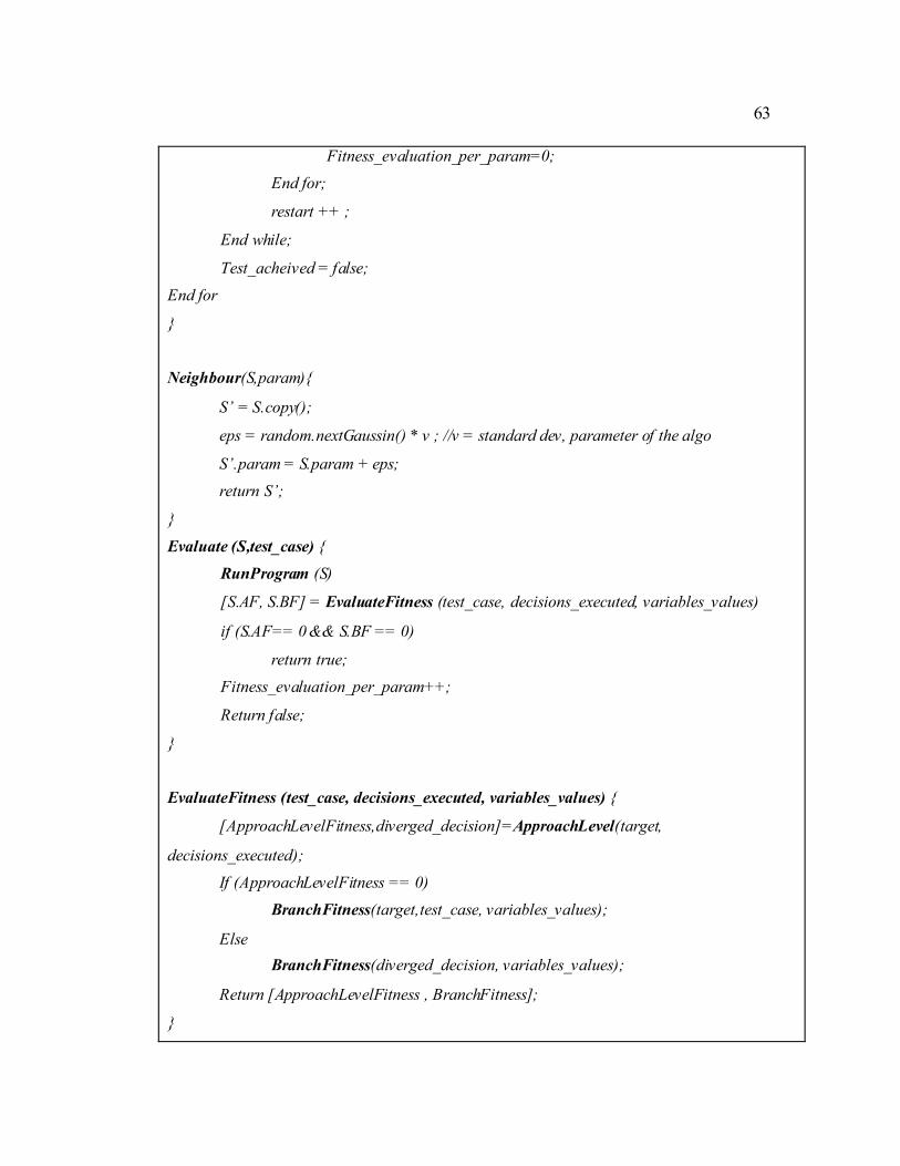
63
Fitness_evaluation_per_param=0;
End for;
restart ++ ;
End while;
Test_acheived = false;
End for
}
Neighbour(S,param){
S’ = S.copy();
eps = random.nextGaussin() * v ; //v = standard dev, parameter of the algo
S’.param = S.param + eps;
return S’;
}
Evaluate (S,test_case) {
RunProgram (S)
[S.AF, S.BF] = EvaluateFitness (test_case, decisions_executed, variables_values)
if (S.AF== 0 && S.BF == 0)
return true;
Fitness_evaluation_per_param++;
Return false;
}
EvaluateFitness (test_case, decisions_executed, variables_values) {
[ApproachLevelFitness,diverged_decision]=ApproachLevel(target,
decisions_executed);
If (ApproachLevelFitness == 0)
BranchFitness(target,test_case, variables_values);
Else
BranchFitness(diverged_decision, variables_values);
Return [ApproachLevelFitness , BranchFitness];
}

64
3.3.2.3. Neighbour Selection
A uniformly generated Є is drawn from a Gaussian distribution with 0 mean and
σ standard deviation. σ is a parameter for the algorithm, thus for different solution space,
the value of σ can differ. A solution can be made of several method parameters; thus its
neighbourhood space can be multi-dimensional. Our neighbour selection technique
would modify one parameter at a time, keeping the others fixed. This way, we make sure
the neighbourhood of each dimension is explored. Thus, we pass the parameter index
param to the Neighbour method, a neighbour S‟ is created as a copy of the current S
solution, then the value of param is modified by Є and updated in S‟.
Figure 3.11: Mutli-dimentional solution
3.3.2.4. Fitness Evaluation
HC evaluates the fitness function for each generated neighbour. Details on the
calculations will be presented in the next chapter. The fitness function of each neighbour
is compared to the fitness of the current solution. If it improved, than the neighbour
replaces the current solution, otherwise the neighbour is dropped and another neighbour
is selected.

65
3.3.2.5. Iterations per Parameter
The search can run up to a maximum number of iterations, after which the search
for the test case is reported as failed if no test datum is found to zero the fitness function.
For a multi-dimensional solution, we explore the neighbourhood of the solution
per parameter at a time. The algorithm is fed with two parameters:
A maximum number fitness_eval_max of allowed fitness evaluation per test case.
A maximum number of restarts max_restart_allowed
Thus, fitness_eval_max is divided by max_restart_allowed to know how many fitness
evaluations can be done in one search iterations before a restart is done. Since we are
searching the neighbourhood of the solution by parameter, then we divide again this
number by the number of the solution‟s parameters to get the maximum allowed fitness
evaluation per parameter Fitness_evaluation_per_param, in other words the maximum
allowed neighbour selection for the current solution.

66
Chapter 4: Our MC/DC Test Automation Approach
4.1. MC/DC Criterion
The MC/DC criterion was developed to provide many of the benefits of
exhaustive testing of Boolean expressions without requiring exhaustive testing
(Hayhurst, 2001).
4.1.1. Definitions
For sake of completeness we report in the following the basic definitions needed
to understand MC/DC and MC/DC test data generation.
A condition is “A Boolean expression containing no Boolean operators”, for
example (a < b).
A decision is “A Boolean expression composed of conditions connected by
Boolean operators. A decision without a Boolean operator is a condition. If a
condition appears more than once in a decision, each occurrence is a distinct
condition” (Hayhurst, 2001). For example, (a < b && a < c) is a decision
composed of two conditions. “&&” is the Boolean operator AND.
Each “if” statement in a code is a decision statement and it contains one or more
conditions.
Other terms that need to be defined are a predicate, major clause and minor clause. A
predicate is a synonym used for condition. Major clause is the condition the test aims to
prove that it affects correctly the outcome of the decision, while the minor clauses are all
other conditions in the decision.
4.1.2. Goal
MC/DC is intended to assure, with a high degree of confidence, that
requirements-based testing has demonstrated that each condition in each decision in the

67
source code has the proper effect on the outcome of the decision (Hayhurst, 2001). The
goal of MC/DC criterion is thus to prove that:
every decision in the program under test has taken all possible outcomes at least
once,
every condition in a decision has taken all possible outcomes at least once,
more importantly that each condition in a decision affects independently and
correctly the outcome of this decision.
A side effect is also that the tester is able to locate where exactly the error is in a
decision, if any.
4.1.3. MC/DC Test Cases
There are two MC/DC variants. In the first one, also referred to as the unique
cause MC/DC, minor clauses must hold the same Boolean value for the two values of
the major clause. The second interpretation of MC/DC, a weaker criterion known as the
masking MC/DC, allows minor clauses to be different (Ammann, Offutt, & Huang,
2003). In this work, we will consider the strongest interpretation, the unique cause
MC/DC, as it is the criterion required by the standard DO-178B.
In order to generate the test suite to cover the MC/DC criterion for one decision,
the major clause value should vary while the minor clauses outcomes are fixed , to show
the effects of the major clause on the entire decision.
Boolean conditions such as a < b are denoted by capital letters representing the condition
outcome (A ,B, C, etc.) and the Boolean outcomes are denoted true (T) or false (F).
To help understanding a decision such as (A and B), logical operators (or, and, etc.) are
presented schematically by logical gates, and a truth table is built for the entire logical
circuit. This truth table represents the truth table for the decision under test.

68
Figure 4.1: Representations for Elementary Logical Gates (Hayhurst, 2001)
Figure 4.1 illustrates the logical “and” and “or” Boolean operators represented by
logical gates. It also provides the truth table for these gates. Each row in the truth table
presents a possible test case, thus in the truth table of the “and” gate for example, we
have four possible test cases for the decision “A and B”. However, when developing test
sets, we want also to minimize the number of test cases required to cover the MC/DC
criterion. Thus, for each major clause, we search for a pair of rows where the condition
outcome varies, the minor clauses outcomes are fixed and the outcome of the entire
decision varies. For the “A and B” truth table, the pairs of rows for each major clause
are:
A: {(TT→T),(FT→F)}
B: {(TT→T),(TF→F)}
Thus the final test set is {(TT), (FT), (TF)}.
As a general rule, a set of n+l test cases is needed to provide coverage for an n-
input decision.

69
Figure 4.2: Calc method
Consider the Java code in Figure 4.2; suppose we are interested in generating
input data to satisfy the MC/DC for the decision at line 16 (z > x && z > y || z > x + y).
We denote the conditions (z > x) by Z1, (z > y) by Z2 and (z > x + y) by Z3, thus the
decision is denoted as (Z1 && Z2 || Z3). We build the truth table of the correspondent
logical circuit.
Table 4.1: Truth table of decision at line 16 of the Calc method
# Z1 Z2 Z3
0 F F F F
1 F F T T
2 F T F F
3 F T T T
4 T F F F
5 T F T T
6 T T F T
7 T T T T

70
Searching the truth table for the pairs of rows for each major clause, we obtain:
Z1: (2,6)
Z2: (4,6)
Z3: (0,1), (2,3), (4,5)
To save space test cases were represented by a decimal coding thus for example
the number 3 stands for FTTT in the truth table. We have two minimal sets to cover the
MC/DC criterion: {2,6,4,3} and {2,6,4,5}. We can choose any one of the two sets.
4.2. The Approach Steps
Results of a 1999 survey of the aviation software industry showed that more than
75% of the survey respondents stated that meeting the MC/DC requirement in DO- 178B
was difficult, and 74% of the respondents said the cost was either substantial or nearly
prohibitive (Hayhurst & Veerhusen, 2001). In fact, the main challenge when trying to
achieve the MC/DC coverage is to overcome the complexity of the code under test; it is
not sufficient to generate test data for a program‟s decisions isolated, rather test data
should be appropriately chosen in order to reach the targeted decisions and to achieve
the relative test cases.
The most common approach to analyse the structure of the code under test is to
extract its control flow graph (CFG). In fact, most of the structural testing approaches
rely on the CFG to measure coverage and guide the search for the test input data. We
can cite as examples the work of Korel in 1990 on branch coverage, the work of Baresel
in 2002 on structural testing using evolutionary testing relying on the CFG to build the
fitness function and the work of McMinn in 2004 also using the CFG to build the fitness
function for branch testing.
4.2.1. Control Flow Graph
A CFG is a graph representing the program structure. The CFG nodes represent
computations. While in some CFG forms, a node represents one statement of code, in
other CFG forms, a node can represent a code segment depending on the convention
used; a segment being one or more lexically contiguous statements with no conditionally

71
executed statements in it (Binder, 2000). Nodes can be named or numbered by any
useful convention.
The edges (also called branches) represent the flow of control, which is usually a
conditional transfer of control between a node and another one. An edge connects two
nodes, representing the entry into and the exit from the statement.
The entry point of a program is represented by an entry node with no incoming
edges. The exit point of a program on the other hand is represented by the exit node with
no outbound edges (Binder, 2000).
The CFG is a essential for the MC/DC testing because the flow of control is
directed by the conditional nodes in the CFG; these nodes being predicate expressions
such as an “if”, “while”, do until”, etc. The CFG of a program is the fundamental
structure required to guide the input data into the correct path to reach a targeted
decision.

72
Figure 4.3: Calc method
Figure 4.4: CFG for the Calc method
The CFG of the Calc() method is shown in Figure4.4. To reach the node 14 for
example, nodes 1 to 3 are traversed, then either the true edge or the false edge of both
decisions nodes 4 and 8 can be traversed. However, the true edges of nodes 12 and 13
must be traversed to reach 14.
4.2.2. Decision Coverage and MC/DC Coverage
Decision coverage, also known as branch coverage, is achieved when each edge
in a CFG is covered, and thus every edge from a decision node is traversed at least once.
Ensuring that all decisions in the CFG are tested at least once implies the necessity to
reach the decisions first. Let us assume that we want to test the decision at line 16 in the
Calc method in Figure 4.4. At a first look at the CFG, we can deduce that the input data
generated must traverse the true branch of the decision at line 12 and the else branch of

73
the decision at line 13 to reach the target decision. We can deduce that our target
decision at line 16 is dependent on the flow of control through the decisions 12 and 13.
We call such dependencies control dependencies. Moreover, a test data diverging away
from the target at line 13 would be closer to the target from a test data diverging at line
12. In general, to automate the search for test data reaching a target statement, we need a
cost function that determines which test data is closer to reach the target node. The cost
function verifies for each test data how many controlling nodes were traversed in the
required manner. The more traversed controlling nodes the better the cost function. This
cost function is the Control Dependencies fitness function.
The problem with the search relying solely on the control dependencies between
nodes is that it ignores prior statements that need to be executed first to make the path
feasible to reach the target. Going back to our targeted decision at line 16, even though
this decision does not appear to depend on decisions at lines 4 and 8, following the CFG,
the outcome of these decisions play a decisive role in reaching our target. In fact, the
variable “result” used at line 12 depends on the true branch of the decision at line 8. In
turn, the decision at line 8 depends on the variable “Fail”, which is modified in the else
branch of the decision at line 4. In general, we say that our target decision has data
dependencies on prior nodes in the program, and thus a cost function for the data
dependencies should also be defined. Such a cost function is called Data Dependencies
fitness function.
As proposed by (McMinn & Holcombe, 2006) for branch coverage, we will
integrate both cost functions for MC/DC coverage. The integrated fitness functions form
the Approach level.
Assuming now that we reach the target decision with a test data xi, then we need
to verify if xi achieves one of the MC/DC test goals. Moreover, if two test data xi and yi
reach the target decision, but none of them achieve an MC/DC condition, a new cost
function is needed to measure which of two test data is closer to achieve the test goal at
the condition. In this case, the evaluation function relies on the structure of the target
decision and the test case at hand. Such an evaluation function is called Branch fitness
function.
74
4.2.3. Steps to Automate the Approach
The rest of the chapter describes the main steps needed to achieve the MC/DC
coverage. In the next section, we expla in the code analysis, how we extract the decisions
and analyse their structure to generate the MC/DC test cases. In the first step, we
perform code analysis via code parsing and expression analysis. In the second step, we
extract the control and data dependencies between the program nodes. In the following,
we discuss in details each step and the three components of our fitness function. In the
third step, we present our code instrumentation module. Code instrumentation is a tool
used to inject tracing information into the code in a way to trace the flow of control for
each input data, as well as collecting variables values at chosen locations in the code.
This module helps us evaluate the fitness function at run time with the generated test
data. In the last section of this chapter, we apply each step on a real program.
4.3. Code Parsing and Expression Analysis
Our code parsing and analysis module assumes code has been developed in Java
and implements expression analysis in several steps. First, code is parsed and an
Abstract Syntax Tree (AST) is constructed. Second, the AST is revisited and sub-trees of
decisions are transformed into a reduced representation, Abstract Decision Tree (ADT).
We discuss these steps in details in the following sections.
4.3.1. Building the Parse Tree
In order to generate test cases and test data for the code under test, we need to
perform lexical analysis and syntax analysis on the code. Lexical analysis reads the
characters in a source program and groups them into a stream of tokens in which each
token represents a logically cohesive sequence of characters, such as identifier, a
keyword (if, while, etc.), a punctuation character or a multi-character operator like :=.
The character sequence forming a token is called the lexeme for the token (Aho, Sethi,
& Ullman, 2000). On top of the lexical analysis, syntax analysis involves grouping the
tokens formed into grammatical phrases that are used by the compiler to synthesize

75
output (Aho, Sethi, & Ullman, 2000). The syntax structure of the output is presented by
a parse tree.
The lexical and syntax analysis is performed in our code parsing module via
JavaCC and JJTree on top of Java 1.5 grammar. First, we generate a top-down parser
using javacc on top on the Java 1.5 grammar. Second, we construct the parse tree of the
code using jjtree. JJTree is a pre-processor for JavaCC that inserts parse tree building
actions at various places in the JavaCC source. The output of JJTree is run through
JavaCC to generate the parser code (Sun Microsystems, Inc., 2007). Next, the parser is
compiled and run on the code to generate the parse tree.
The parse tree is a tree representation of the syntax of the code, where each node
in the tree represents a program node. The most basic class within the tree design is the
Node class. Each element of the syntax is represented by a node. The basic node class
provides a group of constructors and several member functions. Two data members are
provided for the Node object: a pointer to a list of nodes, usually the node‟s children,
and a string, which is generally used to hold the name of the derived class, and thus
usually considered as the node‟s type. As a result, in the parse tree, each node is
identified by its type and linked to its children.
Figure 4.5: GetResult method

76
Figure 4.6: AST for the GetResult method
The generic parse tree of the GetResult method (Figure 4.5) is represented in
Figure 4.6. The “if statment” node represents a decision and its block in the code, the
“Conditional Expression” represents the conditional part (exemple if (result== 0) ), the
“Relational Expression” represents the conditions forming the decision and the
“Statement” node represents the statement “true” or “else” block of the decision.
4.3.2. Building the Abstract Syntax Tree
The parse tree is a generic tree containing all the nodes of the program, and
generated based on the grammar parser. Each node in the tree can have up to n direct
children (If statment id: 4) read from left to right. Since the generation of the test cases
for MC/DC requires a clear division of the decisions structure, we need to transform the
parse tree into a more adequate structure. A useful starting point is a translation into an
Abstract Syntax Tree (AST) in which each node represents an operator (i.e. , boolean
operators) and the children of the nodes represents the operands (i.e. , relational
expressions). AST differs from parse trees because superficial distinctions of for m,

77
unimportant for the problem at hand, do not appear in AST (Aho, Sethi, & Ullman,
2000). An example of the translation is shown in Figure 4.7.
Figure 4.7: a) Parse tree b) AST of statement 10 of the GetResult method
4.3.3. Building the Abstract Decision Tree
The resulting AST still contains all the program nodes of the code under test.
However, we are only interested in extracting the decisions logical structure, in fact
logical structure is the sole information required to generate MC/DC sets. Thus, we write
an AST visitor that collects only the subtrees of the decisions such as “if”, “while, “for”,
etc. For example in Figure 4.6, the visitor collects the children of the Condtional Exp.
nodes of the “if” statement, and drops the subtrees of the Statements nodes. Moreover,
Boolean conditions such as x < y are denoted by capital letters representing the
condition outcome and the relational expressions nodes are also denoted by capital
letters representing their outcome. The new generated subtrees are called Abstract
Decision Trees (ADT). Each decision has an ADT representing its logical structure. The
ADTs of the GetResult method are shown in Figure 4.8.

78
Figure 4.8: ADTs of the GetResult method
4.4. MC/DC Test Cases Generator Module
4.4.1. Pseudo-Algorithm of the MC/DC Test Cases Generator
The ADTs form the input for an MC/DC generator and a grammar is used to
analyse the syntax of the trees. Each node in the ADTs is assigned a Boolean value
(either 1 or 0) and a Boolean variable Evaluated, to verify if the node value has already
been computed. A high level pseudo-code of the algorithm is represented in the
following:
Extract the conditions from the trees. The conditions form the leaves of the
ADTs. Let N be the number of extracted variables.
Construct a truth table (TT) of size (N, 2N), since for N variables, we have 2
N
possible combinations.
Populate the TT by alternating for each column the True and False values each
2column
rows.
For each TT row:
o Reset the trees nodes values to 0.
o Assign the current row values to the leaf variables.
o Evaluate recursively bottom up the values of the nodes till reaching the top
of the tree. This value represents the output of the decision being evaluated.
o Update the truth table output column with the resulting value.
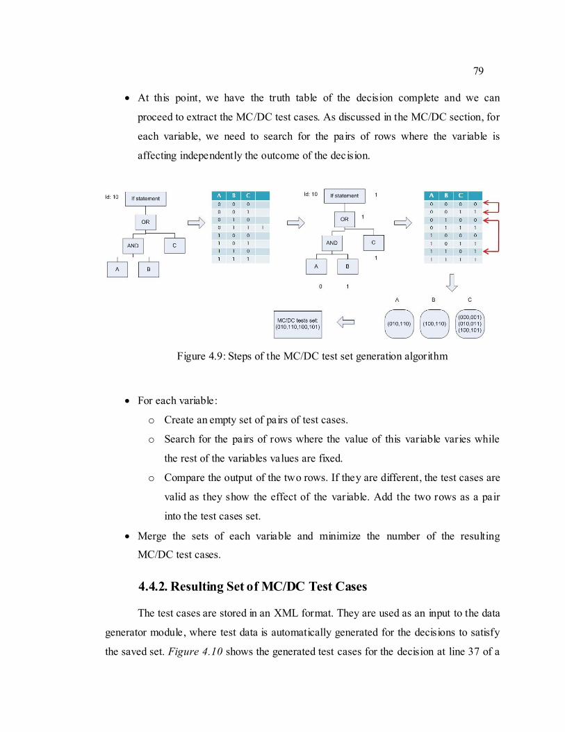
79
At this point, we have the truth table of the decision complete and we can
proceed to extract the MC/DC test cases. As discussed in the MC/DC section, for
each variable, we need to search for the pairs of rows where the variable is
affecting independently the outcome of the decision.
Figure 4.9: Steps of the MC/DC test set generation algorithm
For each variable:
o Create an empty set of pairs of test cases.
o Search for the pairs of rows where the value of this variable varies while
the rest of the variables values are fixed.
o Compare the output of the two rows. If they are different, the test cases are
valid as they show the effect of the variable. Add the two rows as a pair
into the test cases set.
Merge the sets of each variable and minimize the number of the resulting
MC/DC test cases.
4.4.2. Resulting Set of MC/DC Test Cases
The test cases are stored in an XML format. They are used as an input to the data
generator module, where test data is automatically generated for the decisions to satisfy
the saved set. Figure 4.10 shows the generated test cases for the decision at line 37 of a
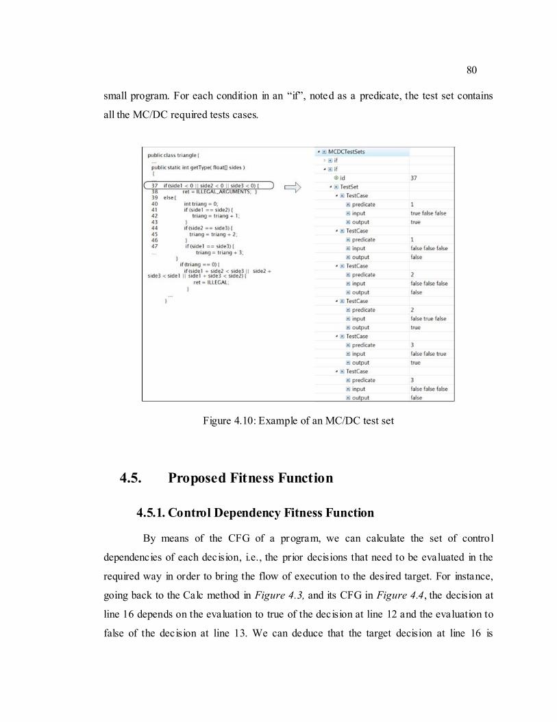
80
small program. For each condition in an “if”, noted as a predicate, the test set contains
all the MC/DC required tests cases.
Figure 4.10: Example of an MC/DC test set
4.5. Proposed Fitness Function
4.5.1. Control Dependency Fitness Function
By means of the CFG of a program, we can calculate the set of control
dependencies of each decision, i.e., the prior decisions that need to be evaluated in the
required way in order to bring the flow of execution to the desired target. For instance,
going back to the Calc method in Figure 4.3, and its CFG in Figure 4.4, the decision at
line 16 depends on the evaluation to true of the decision at line 12 and the evaluation to
false of the decision at line 13. We can deduce that the target decision at line 16 is

81
dependent on the flow of control through the decisions 12 and 13. These nodes are
called critical branches as they determine the flow of control towards or away from the
target (Korel, 1990). Consequently the set of control dependencies for the decision at
line 16 includes the decisions of line 12 and 13, i.e., these are the branching nodes that
must be executed with a specific outcome in order for the target to be reached. We write
ControlDep(16) = {12,-13}; where ControlDep is the set of control dependencies for the
decision at line 16, and it includes a dependency on the true branch of 12 and a
dependency on the false branch of 13.
In general, the term control dependency is used to describe the reliance of a node
execution on the outcome at previous branching nodes (Ferrante, Ottenstein, & Warren,
1987). More formally, a node z is post-dominated by a node y in G if and only if every
path from y to the exit node e contains z. Node z post-dominates a branch (y, x) if and
only if every path from y to the exit node e through (y, x) contains z. The node z is
control dependent on y if and only if z post-dominates one of the branches of y, and z
does not post-dominate y (McMinn, 2004).
Once the control dependencies set is formed, the search needs to reward test
data that execute the greatest number of controlling decisions. For instance, a test data
diverging away from the target at line 13 would be closer to the target than a test data
diverging at line 12. In general, we need an evaluation function that would evaluate
which test data is closer to reach the target. Such an evaluation function is called Control
Dependencies fitness function.
The Control Dependencies fitness function is an objective function that
considers the branching nodes included in the control dependencies set. Let
dependentdecisions be the number of nodes in the ControlDep set of our target, and let
executeddecisions be the number of nodes in the ControlDep set that is actually executed in
the required manner with the current input data. Thus, the control dependency fitness
function to minimize is defined as:
ControlDepFittestdata = dependentdecision - executeddecisions
If the function is zero, the test data reached the target decision. However, if the

82
function is greater than 0, the test data is known to have diverged at a critical branch
away from the target, exactly at the node preceding the target by the amount of the
fitness function. We will call this node divergednode. For instance, in the Calc method,
the input diverging at node 12 (nodes 12 and 13 both not executed as required) will have
the fitness evaluation to 2 - 0 = 2, however the input diverging at node 13 (node 12 being
true as required), will have the fitness equal to 2 - 1 = 1. In this case, the algorithm is
able to distinguish different test input data based on their level of approach from the
target, and the search is guided into the closer input data.
4.5.2. Data Dependency Fitness Function
Going back to our targeted decision at line 16 in the Calc method, even though
this decision does not appear to depend on decisions at lines 4 and 8, according to the
CFG, the outcome of these decisions play a decisive role in reaching our target. In fact,
the variable “result” used at line 12 depends on the true branch of the decision at line 8
which in turn depends on the flag “Fail” modified in the else branch of the decision at
line 4. In this case, the Control Dependency Fitness function provides no guidance at all
on how to make the “Fail” flag false and how to make the “result” variable equal to zero;
the search landscape is completely flat.
This fact is at the basis of the Korel chaining approach (Korel, 1990) and the
McMinn extension (McMinn & Holcombe, 2006). In the later work terminology, line 12
is called a problem node; in a similar way we call “result” a problem variable because
the lacking of knowledge on “result” can cause the search to behave as a random search.
In such cases, we say that our target decision has data dependencies on prior nodes in the
program.
To avoid random search, McMinn and Holcombe in 2004 and 2006 suggest
including “result” data dependencies in the fitness evaluation (McMinn & Holcombe,
2006), ignoring however the control dependencies that the data dependency nodes might
in turn have. For instance, “result” definition at Calc line 10 is controlled by the decision
at line 8; much in the same way, “Fail” definitions (lines 5 and line 7) are controlled by
the decision at line 4. Because dependencies determination presented in the work of

83
McMinn and Holcombe focuses only on data dependencies, control nodes 8 and 4 are
not considered. We believe that explicitly incorporating control nodes such as nodes 8
and 4 into the approach level fitness leads to an easier implementation and an improved
performance.
3.5.2.1. The Pseudo-Code of the Extended Dependencies
Algorithm
Figures 4.11 and Figure 4.12 report our extension of the algorithm of McMinn.
In our approach we aim at collecting control nodes either directly or indirectly (i.e., via
data dependencies) affecting the traversal of the problem node.
Figure 4.11: Algorithm to calculate the sets of dependencies given a problem statement

84
Figure 4.12: Algorithm to calculate the sets of dependencies given a problem statement
The functions getControlDep and getUsedVariable return the set of reverse
control dependencies (nodes controlling the current node) and used variables
respectively. S and DepSets are initialized as empty sets. DepSets stores the set of
dependencies for a given problem node. At algorithm termination, these sets of
dependencies are merged by algorithm in Figure 4.12 to build the sets of dependencies
used in defining fitness functions.
There are two main differences with the Chaining approach of (McMinn &
Holcombe, 2006). First, our test data generation code is written in Java and thus we can
take advantage of Java multi-threading nature: for each last definition of variables
involved in the problem node we store its dependencies (line 14 in Figure 4.11); the
algorithm in Figure 4.12 merges the sets of dependencies and each merged set leads to a
different fitness function run in parallel into its own thread. More conceptual is the
difference in computing dependencies. We perform a closure similar to the Chaining
approach but we are interested in extending the level approach by interleaving control
dependencies and data dependencies to improve the guidance provided by the approach
level fitness.
Again in the Calc method, consider for example line 12 (problem node); “result”
last definition at line 10 causes line 10 control dependence, line 8, to be added to S. At
the algorithm termination, both lines 8 and 4 will be in S.

85
Figure 4.13: Example of multiple flags
More in details consider the part of the program presented in Figure 4.13. We
assume that global variables such as “errno” are modeled as extra parameters. We will
go through the getDependencies algorithm (Figure 4.11) for this piece of program.
The function getControlDep returns the empty set when the method declaration
first line (line 0) is passed. getUsedVariables called on the same line also returns
the empty set.
Suppose that line 10 in the program is the target statement; the problem node
(line 9) uses flag variables “error1” and “error2”.
When called with parameters 12 and φ, the function getDependencies, first
identifies used variables (“error1” and “error2” at line 3) and then computes for
each used variables the last definition set. For example, for “error1” last
definition is line 6.
Last definition is controlled by the decision at line 5 and thus line 5 is added to S
(line 7 in the algorithm).
The decision at line 5 uses the variable “r1” that is added to newPV (new
problem variables). “r1” has two definitions points either at line 2 (then branch)
or line 4 (else branch).

86
getDependencis recursion called over node 5 and S = {5} generates a last
definition set for “r1” of {2, 4}.
The cycle at line 6 in the algorithm iterates over {2, 4}.
Suppose that line 2 (then branch) is selected (line 6 in the algorithm) then line 7
adds line 1 to S.
Notice that in the case of an else branch (e.g., last definition at line 4 in the
program), getControlDep returns minus the control node number; negative
values encode last definitions in the else branch. In essence, we encode with
positive numbers the control flows going into then branches while negative
values stand for else branches.
Recursion of getDependencis with parameters 1, {5, 1}, will check “b” last
definition leading to line zero, method definition first line. Line zero in our
model has no control dependencies and uses no variables.
Both newPV and getControlDeps(0) are the empty sets and set {5, 1} is added to
DepSets, line 14 in the algorithm.
The same way, the set {5,−1} is added to DepSets.
Finally, when getDependencies computes “errno” induced dependencies, the set
{7} is added to DepSets.
Overall, the call to the function getControlDeps(9, φ) generate the sets: {{5, 1},
{5,−1}, {7}}.
At this point, DepSets is now the input to the algorithm in Figure 4.12 that generates
the actual new set of dependencies for fitness definition. The function
thenElseConflicts(si, sj) returns true if a set contains both the then and the else branch of
the same decision. Therefore when the algorithm is executed over the set {{5, 1},
{5,−1}, {7}} it generates the sets of dependencies: {φ, {5, 1}, {5,−1}, {7}, {5, 1, 7},
{5,−1, 7}}. Overall, six fitness functions one for each set in DepFit are defined and six
threads will be started probing various combination of control flow to cover line 9
MC/DC. For example, the set {5,−1, 7} is interpreted as: we need to enter the “else”
branch of line 1, and the “then” branch of line 5 and line 7.

87
We believe that this extending of the approach level, which includes the data
dependencies, improves the guidance of the search towards more promising search area
for test data. The new extended approach is intended to overcome the problem of lack of
guidance and flat search when flag variables are used at predicates or when strong data
dependencies exist between the predicates of the code.
4.5.3. Branch Fitness Function
Once the test data reaches the target, it needs to satisfy one of the MC/DC test
cases. However, for individuals not satisfying any of the MC/DC test cases, no guidance
is given as to how to descend down the landscape to solutions that are closer to
achieving one of the test cases (McMinn P. , 2004). Along these horizontal planes, the
search becomes random. Thus, we need another measurement to verify if the test data
satisfied a test case, and if not, how close it is from satisfying it. The value obtained is
called “branch distance”.
For a given program, every test data diverging away from the target at node x
receives the same approach level value. However, a branch distance calculation is
performed at the diverging node, to evaluate which of the test data is closer to satisfy it
(make it true or false according to the control dependency set). If every test data reaches
the target decision but none achieves one of the MC/DC test cases, every test data will
have a zero approach level. However, a branch distance calculation is performed at the
target decision to evaluate which of the test data is closer to satisfy one of the test cases
at this node. Of course, if a test data reaches the target and achieves one of the MC/DC
test cases, then its branch fitness as well as its approach fitness would evaluate to zero.

88
Table 4.2: Conventional cost functions for relational predicates (Bottaci, 2001)
Table 4.3: Modified relational predicate cost functions (Bottacci, 2003)
Table 4.4: Our extended branch fitness
The branch distance at a decision is calculated based on the structure of this
decision. A work done by Bottacci in 2001 provides fitness formula for all possible
logical operations in a decision. In Table 4.2 (P small positive number and L very large
positive number), the initial functions are only applicable for the true branch of a
decision. In 2003, Bottacci extended these formulas to cover the else branch as well. The
extension used an arbitrary value R, being a minimum absolute cost for any predicate, to
differentiate the “then” and the “else” branch, R is added to the value of the fitness for
the “then” branch, and subtracted from the value of the fitness for the “else” branch,

89
shown in Table 4.3 (Bottacci, 2003). We believe that a ternary operator representing the
conditional expressions would better extend the initial functions as no arbitrary values
are added. The extended branch fitness formulas are shown in Table 4.4.
Branch fitness is always a positive value. When trying to achieve a test case, we
compare the closeness of the test data to achieve the test case, rather than the value of
the test data itself. Thus, a negative value of the fitness function would not add any
valuable information to the search. Thus, an absolute value is applied to the value of the
branch fitness before it is returned.
4.5.3.1. Example of the Branch Fitness Calculation
Considering the Calc method again in Figure 4.2, suppose our goal is to generate
test cases to satisfy MC/DC for line 16: if (z > x && z > y || z > x + y). Suppose also that
we want to satisfy the test case (TFF), which means the condition z > x should be true,
and the two conditions z > y and z > x + y should be false. Numbers 0 and 1 are used to
represent false and true; they are interpreted as real values simplifying fitness evaluation
i.e., distance from the sought value assignments. If two different test cases reach line 16,
we need to decide which one of them is the most promising one to obtain (100). Thus,
we need to evaluate the branch fitness for each test data, using the “then” branch fitness
for z > x and the “else” branch fitness for z > y and z > x + y, the formulas being
presented in Table 4.5. The overall branch fitness function is then computed based on
the addition of the branch fitness functions of each condition in the decision. We show
in the last section in this chapter a detailed calculation for real test data.
Table 4.5: Calc line 16 branch fitness computation
Expression Then branch Else branch
fit(z > x) abs(z > x?0 : z − x + k) abs(z > x?z − x + k : 0)
fit(z > y) abs(z > y?0 : z − y + k) abs(z > y?z − y + k : 0)
fit(z > x + y) abs(z > x + y?0 : z − x − y + k) abs(z > x + y?z − x − y + k : 0)

90
4.6. Code Instrumentation Module
The code instrumentation module is a parsing tool used to instrument the code
under test and extract relevant information. In the reverse engineering terms, code
instrumentation relies on “unparsing” techniques. At a first step, the code is parsed using
the parsing technique presented in section 4.3.1 (building the parse tree), preserving all
comments and white space. Then, the parse tree generated is annotated with
instrumentation; the required nodes to be instrumentation are located in the tree, and the
printing of the node is modified to inject tracing information in the code. The
instrumented tree is then unparsed and the initial code is regenerated with the new
tracing information injected in it.
The Approach Level fitness requires the collection of the executed decisions in
the code for each test data. Thus, when the program is executed for an input test data xi ,
the instrumentation module should be able to analyse the flow of execution of the
program and collect the decisions that were executed. Without this information, it is
impossible to evaluate the Approach Level Fitness.
Table 4.6: Instrumentation of a decision
If (node.Is(ASTIFStatement) )
If (node.child.Is(ASTElseBranch) )
Print (- node.line);
Else
Print (node.line);
End if
For this reason, in the code unparsing, every time a decision node is encountered,
a printout needs to be inserted in the “then” and “else” branch of the decision as shown
in Table 4.6. If the “then” branch is executed, a number representing the line of the
decision is printed and the decision is known to have been executed to true. If the “else”
branch is executed; a negative number representing the line of the decision is printed.

91
This kind of collected information helps building the ExecutedDecisions set and thus
evaluating the Approach Level.
The branch fitness function needs to be evaluating either at the diverging
decision or at the target decision, we call either of the decision dt. As discussed above,
the branch fitness formula is dependent on the structure of dt. Once the fitness formula is
built, it needs to be evaluated with the current variables values at dt. However, for
different test input data, the program might have different flow of execution and thus the
variables used at dt might be evaluated much differently. The code instrumentation tool
provides the technique to extract the values of the variables at run time for each test data
executed on the program.
Table 4.7: Instrumentation of variables at decision nodes
If (node.Is(ASTVar) )
If (node.parent.Is(ASTIFstatment) )
Print (getValue(node.name, node.data , node.line) );
End if
If(node.Is(ASTClassOrInterfaceBodyDeclaration) )
Print (“getValue(node_name, node_value, node_line) {
Print (<decision id: node_line>
<variable name:node_name>node_value</variable>
</decision> )
End if
Table 4.7 shows the pseudo-code for the instrumentation. If a variable in a decision
is encountered during the parsing, it is reprinted with an injected getValue() method. The
getValue() method is also inserted in the body of the program, it prints the name of the
variable, the decision line in which it occurred and more importantly the value of the
variable at run time.

92
4.7. Overall Fitness Function Evaluation
To evaluate the fitness function for a test input data, the instrumented program
under test is executed with the test data. The information collected for each execution is
the set of decisionExecuted and the set of variablesValues at the target decision or at the
diverged node. These two sets are fed into an evaluation method that will start by
calculating the ApproachLevelFitness function. If the ApproachLevelFitness is zero,
then the test data reached the target and thus the BranchFitness is calculated at the target
decision with the set of variablesvalues. If the ApproachLevelFitness is greater than
zero, then the test data did not reach the target and the BranchFitness is calculated at the
diverging node. If the ApproachLevelFitness and the BranchFitness are both zero, then
the test data achieved an MC/DC test goal. Otherwise, the fitness function of the test
data will be equal to ApproachLevelFitness + normalized(BranchFitness), normalization
of BranchFitness to make it between 0 and 1.
We present in the following an example of fitness function calculations for the
Calc method in figure 4.2. We assume that our target decision is at line 16.
4.7.1. Preliminary Phase Activities
The control depedency set of this decision is: {12,-13}.
The sets of data dependencies for this decision are: {φ,{2},{2,3,4,8},{2,3,-4,8}}.
The sets of dependencies are thus: {φ,{2,12,-13},{2,3,4,8,12,-13},{2,3,-4,8,12,-
13}}. The fitness function for each set runs in parallel threads. In this example,
we consider the thread of the dependency set {2,3,-4,8,12,-13}.
The MC/DC test cases extracted from the MC/DC test cases generator in section
4.1.3 for the target decision at line 16 in the Calc method were:
{(010,110,100,011}. In this example, we will aim to achieve the test case (010).
The target decision is: if (z > x && z > y || z > x + y).

93
4.7.2. Calculations on the Fly
Assume now that at run time the test data generator outputs two test data (12,-
2,3) and (1,2,0) for the parameters x, y and z of the Calc method. The approach needs to
evaluate the fitness function for these two test data in order to verify if one of them
satisfies or is close to satisfy the MC/DC test case (010).
Test input data T1=(12,-2,3):
Because the goal is to traverse to the else branch of the decision at line 4, we applied
the else branch formulas to the branch distance. Also, the branch fitness is always
positive.
Test input data T2 = (1,2,0):
Because the goal is to traverse to the else branch of the decision at line 13, we
applied the else branch formula for the equality. We choose k =0.1 in this case.
Normalisation of the branch fitness
Comparison of the test data

94
→ T2 is closer to reach the decision target.
Assume now that the data generator outputs the test data (4,7,3) alone.
Test input data T3 = (4,7,3)
The ApproachLevelFitness is zero; the test data reached the target. Since there is
only one test data, that there is no need to normalize the BranchFitness. The test case to
achieve is 010, thus we want (z < x) to be false, (z > y) to be true and (z > x+y) to be
false.

95
Chapter 5: Experimental Study and Results
In this chapter, we report results from a preliminary experimental study carried
out to evaluate the performance of our approach for MC/DC automatic test input data
generation using GA. The GA based approach is compared to two other searching
strategies: random search (RND) and HC. In the next subsections, we briefly describe
two Java programs used as test beds, the hypotheses, and the main experimental steps,
details about the algorithmic settings, and finally, we present results and their
interpretation.
5.1. Subject Programs
The first program is a triangle classification program (Triangle) which is a well-
known problem used as a benchmark in many testing works.
Figure 5.1: Fragment of the Triangle program
This program takes three real inputs representing the lengths of triangle sides and
decides whether the triangle is irregular, scalene, isosceles or equilateral. It counts 80
lines of code; the complete program code is presented in the Annexe of the thesis.
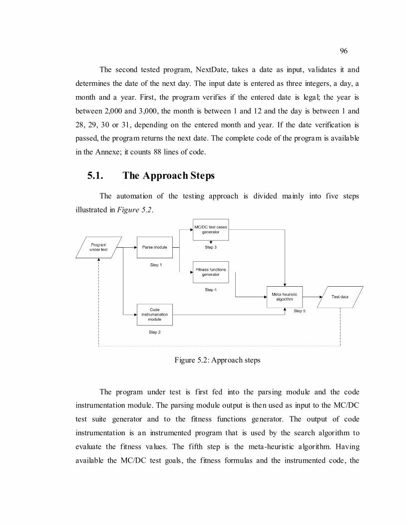
96
The second tested program, NextDate, takes a date as input, validates it and
determines the date of the next day. The input date is entered as three integers, a day, a
month and a year. First, the program verifies if the entered date is legal; the year is
between 2,000 and 3,000, the month is between 1 and 12 and the day is between 1 and
28, 29, 30 or 31, depending on the entered month and year. If the date verification is
passed, the program returns the next date. The complete code of the program is available
in the Annexe; it counts 88 lines of code.
5.1. The Approach Steps
The automation of the testing approach is divided mainly into five steps
illustrated in Figure 5.2.
Figure 5.2: Approach steps
The program under test is first fed into the parsing module and the code
instrumentation module. The parsing module output is then used as input to the MC/DC
test suite generator and to the fitness functions generator. The output of code
instrumentation is an instrumented program that is used by the search algorithm to
evaluate the fitness values. The fifth step is the meta-heuristic algorithm. Having
available the MC/DC test goals, the fitness formulas and the instrumented code, the
97
algorithm starts its search for the test data to achieve the set of test cases for each goal
and each decision in the tested code.
5.2. Algorithmic Settings
We present in the following sections the algorithmic settings for each of the GA,
HC, and the RND algorithms. The first section presents the common settings of the three
algorithms and the following sections detail the specific sections of each algorithm.
5.3.1. Common Settings
5.3.1.1. Stopping Criterion
The sole common parameter between RND, HC and GA is the termination
criterion MaxNbrEvaluation. Based on several runs, we observed that 5,000 fitness
evaluations were usually sufficient to decide if the MC/DC coverage was attainable
given the predicate and the algorithm initialization (single point for HC, initial
population for GA). However, we were also interested to see the effect of the fitness
evaluations on the coverage attained for each algorithm. Thus, MaxNbrEvaluation was
set to 5,000 fitness evaluation per test case for a first experiment, and then it was
increased to 10,000 maximum fitness evaluations for a second experiment.
5.3.1.2. A Solution
For both tested programs, a solution is a three integer input data. Thus the three
algorithms, GA, HC, and RND, generate a triplet of integers as evolving solutions each
iteration. This is a special case, however the three algorithms supports integers and
floats.
5.3.2. Genetic Algorithm
For GA, the elitist strategy was used; each iteration the entire population was
replaced, except for the fittest individual (i.e., test data). The number of individuals in a
generation is set to 100. We set an overall maximum number of GA generations of 400;

98
this is to say that either the computation is halted after the maximum allowed number of
fitness evaluations or after 400 generations per test case.
The values of pc (crossover probability) and pm (mutation probability) are set to
0.70 and 0.05 respectively. We use a whole-arithmetic crossover technique with an α
uniformly drawn from a normal distribution with zero mean and standard deviation
equal to 1. The mutation technique used is a uniform mutation.
5.3.3. Hill Climbing
To select a neighbour, a parameter is incremented and decremented by a step
uniformly drawn from a Gaussian distribution with zero mean and standard deviation σ.
We set 100 total iterations for HC. For the fitness evaluation limit of 5,000, each
iteration, 100 neighbours of each parameter are explored. For the fitness evaluation limit
of 10,000, 200 neighbours of each parameter are explored. This allows us to perform 16
random restarts of the search in no input data is found to achieve the test goal.
The standard deviation σ is changed for different input domain. For the triangle
program, it is set to 400 for the entire integer domain. For the NextDate program, σ is set
to 5 for the days, 10 for the month and 50 for the years, since the domain space for days,
months and years is set to 50, 500 and 4,000 respectively. The domain space in this case
is bigger than the acceptable input domain (12 month, 30 days and 2000 years);
however, we wanted to test the program with non acceptable parameters to verify its
behaviour.
5.3.4. Random Generator
We compare our results to the most trivial data generator, the random generator
RND. It randomly generates a triplet of integers and evaluates the fitness value for this
triplet using the same set of test cases and fitness functions. If the fitness value is zero,
the generated data achieved a test goal, it is returned and a new test goal is selected. If
the fitness value is not zero, the algorithm does not use this value to guide its search;
rather it just generates randomly a new triplet. The maximum number of iterations is set
to the same used for HC and GA.

99
5.4. Results for the Triangle Program
For each of the two exemplary programs, each algorithm computation was
repeated 30 times using the traditional fitness function (without integrating data
dependencies into the fitness function) and using the proposed fitness function (with
integrating data dependencies into the fitness function) for GA and HC. The goal is to
show the MC/DC coverage for the two programs under test for both fitness functions.
5.4.1. Results Without Integrating Data Dependencies
Several experiments were conducted on the MC/DC coverage for the Triangle
program. First, we studied the impact of the parameters domain space on the automation
of the search for the test data. Then, we studied the impact of the number of search
iterations on the data generation as well. The data generation measurement is reported
by the percentage of MC/DC test cases that were achieved by the generated test data.
5.4.1.1. Impact of the Parameters’ Domain Space
The fitness evaluation is set to a maximum to 5,000 evaluation per test case for
this experiment.
Figure 5.3: Results for Triangle program without integrating data dependencies in the
fitness function (maximum of 5,000 fitness evaluation)

100
Table 5.1: Results for Triangle program without integrating data dependencies in the
fitness function (maximum of 5,000 fitness evaluation)
Input domain GA (%) HC (%) RND (%)
-100,+100 95.0 95.0 90.0
-1000,+1000 83.0 95.0 68.0
-2000,+2000 81.0 86.0 63.0
-4000,+4000 75.0 80.9 54.0
-8000,+8000 69.9 76.7 47.1
-16000,+16000 64.2 60.1 44.7
-32000,+32000 56.8 47.4 43.1
Integer domain 54.7 39.0 40.0
Figure 5.3 reports the performance of RND, HC and GA for various dimension
of the search space. Triangle takes three integers and decides the kind of corresponding
triangle. The results show that the larger the input parameter domains the lower the
attained average MC/DC coverage. As shown in Table 5.1, when the parameters range
between plus or minus 100, even a simple random search attains an average of 90 % of
MC/DC coverage. The reason is that the number of fitness evaluation is high (i.e., 5,000
per test case) and the entire search space is explored.
However, as the dimension of the search space increases (up to the integer
range), the coverage for the three searching strategies decreases. For example, GA drops
to 55 % and HC to 39%, performing as a random search. RND drops quickly to 68% for
an input domain of -1000 to 1000, and gets as low as 40% for the integer domain. HC
performs better for small input domain, attaining a better coverage percentage than GA
for input domain lower than |8,000|, but then degrades to perform as a random search for
higher inputs.

101
Table 5.2: Coverage per program decision for the entire integer domain (maximum of
5,000 fitness evaluation)
Decision GA (%) HC (%) RND (%)
37 100.0 96.6 100.0
41 100.0 53.5 50.0
44 98.3 53.5 50.0
47 98.3 55.7 50.0
50 50.0 53.5 50.0
51 100.0 72.4 100.0
57 0.0 0.0 0.0
60 0.0 0.0 0.0
63 0.0 0.0 0.0
66 0.0 0.0 0.0
Total 54.7 38.5 40.0
The reason for such performance degradation is in the equilateral and isosceles
triangle types. First and foremost, equilaterals and isosceles triangles imposes hard
constraint and, sampling out of the entire integer space, the probability to obtain the
same number repeated two or three time is very low.
A second reason is related to the structure of control and data dependencies of
the Triangle program. Table 5.2 reports the details of average MC/DC coverage for the
decisions in the Triangle program shown in the excerpt of Figure 5.1 for the entire
integer input domain. The traditional fitness function has zero coverage for the critical
nodes at lines 50, 51, 57, 60, 63 and 66. As shown in the Triangle code excerpt, the
decision at line 57 has a reverse control dependency from the “if” at line 50, and both
have data dependencies on lines 42, 45 and 48. These lines in turn are controlled by the
“if” at lines 41, 44 and 47 respectively. In other words, a fitness function based on the
standard approach level and branch distance has no guidance to reach the line 57 and
thus the three “if” controlled by line 57, for example, the “if” at line 60. Thus the code

102
section deciding if the triangle is equilateral or isosceles is extremely difficult to reach if
the search space is large and not entirely explored by the search algorithm. Indeed, these
three “if” are not reached by RND, HC or GA within 5,000 fitness generations searching
into the 32 bits integer range. This is the reason why in Figure 5.3 we observe the drop
in MC/DC coverage.
5.4.1.2. Impact of the number of Search Iterations
The same experiment is conducted again with a maximum number of allowed
fitness evaluations of 10,000. Again, the data dependencies are not included in the
fitness function. The results of the experiment are shown in Figure 5.4. The performance
of the three algorithms GA, HC, and RND is then compared with the results of the first
experiments in Figure 5.5, 5.6, and 5.7.
Figure 5.4: Results for Triangle program without integrating data dependencies in the
fitness function (maximum of 10,000 fitness evaluation)

103
Table 5.3: Results for Triangle program without integrating data dependencies in the
fitness function (maximum of 10,000 fitness evaluation)
Input domain GA (%) HC (%) RND (%)
-100,+100 99.7 96.7 96.0
-1000,+1000 88.7 93.4 88.4
-2000,+2000 85.8 90.1 67.0
-4000,+4000 85.1 86.3 60.1
-8000,+8000 82.8 85.4 58.4
-16000,+16000 80.4 64.6 51.6
-32000,+32000 77.6 63.2 46.7
Integer domain 54.9 37.3 40.0
Figure 5.5: Impact of fitness evaluation on GA - without data dependency

104
Figure 5.6: Impact of fitness evaluation on HC - without data dependency
Figure 5.7: Impact of fitness evaluation on RND
Results in Figure 5.5, 5.6 and 5.7 show that for small input domain, the three
algorithms perform better with a higher number of fitness evaluations. Moreover, with
higher input domain, the impact of the evaluations becomes bigger in the case of GA

105
and HC. For example, GA covers 77% vs. 57% for an input domain of 32,000; for the
same domain, HC covers 63.2 % vs. 47.4%. Still, we can see that when the input domain
becomes the entire integer space, even with a fitness evaluation of 10,000, the search
degrades to the coverage of a random search; GA covers 54.9%, HC covers 37.3% and
RND covers 40%.
5.4.2. Results with Integrating Data Dependencies
We run again both experiments with maximum fitness evaluation 5,000 then
10,000, however this time using our new fitness function having the data dependencies
integrated in it. We present first the results of the first experiment and we compare its
results with the previous results without data dependencies.
Figure 5.8: Results for Triangle program with data dependencies in the fitness function
(maximum of 5,000 fitness evaluation)

106
Table 5.4: Results for Triangle program with data dependencies integrated in the fitness
function (maximum of 5,000 fitness evaluation)
Input domain GA (%) HC (%) RND (%)
-100,+100 95.0 96.0 90.0
-1000,+1000 93.0 96.0 68.0
-2000,+2000 91.0 96.0 63.0
-4000,+4000 90.0 93.0 54.0
-8000,+8000 86.6 86.0 47.1
-16000,+16000 85.0 72.0 44.7
-32000,+32000 83.6 59.0 43.1
Integer domain 81.0 48.4 40.0
Figure 5.8 summarizes the results obtained for the Triangle program with the
new fitness function including data dependencies for a maximum fitness evaluation of
5000. Though HC performs best for small input domain, GA largely outperforms HC for
larger domains; this is likely due to the neighbourhood definition that needs to be
improved to cope with large search spaces. Overall, data dependencies have a lower
impact on HC attained coverage.
Table 5.5: a) Input domain -16000 to 16000 b) Entire integer domain
Decision
GA
(%)
Old
GA
(%)
HC
(%)
Old
HC
(%)
RN
D (%
)
37 100.0 100.0 100.0 100.0 100.0
41 100.0 100.0 91.4 82.8 51.7
44 100.0 100.0 87.9 89.7 50.0
47 100.0 100.0 89.7 91.4 51.7
50 86.2 86.2 55.2 60.3 56.9
51 100.0 100.0 100.0 100.0 100.0
57 82.8 46.6 27.6 15.5 10.3
60 79.3 51.7 59.8 24.1 11.5
Decision
GA
(%)
Old
GA
(%)
HC
(%)
Old
HC
(%)
RN
D (%
)
37 96.6 100.0 94.0 96.6 100.0
41 100.0 100.0 53.0 53.5 50.0
44 94.8 98.3 53.5 53.5 50.0
47 100.0 98.3 55.5 55.7 50.0
50 60.3 50.0 55.0 53.5 50.0
51 100.0 100.0 73.3 72.4 100.0
57 86.2 0.0 100.0 0.0 0.0
60 57.7 0.0 0.0 0.0 0.0

107
63 85.1 49.4 52.9 21.8 5.7
66 66.7 33.3 57.5 14.9 9.2
Total 90.0 76.7 72.2 60.1 44.7
63 56.3 0.0 0.0 0.0 0.0
66 55.2 0.0 0.0 0.0 0.0
Total 81.0 54.7 48.4 38.5 40.0
On the other hand, GA with integrated data dependencies performs substantially
better than approach level and branch distance alone. In fact, GA covers 81% vs. 54%
for the entire integer domain, which is a 30% gain, obtained due to data dependencies.
Indeed, the new fitness outperforms the old one in the code region controlled by the
statement 57 as shown in Table 5.5 a) and b). Table 5.5 a) shows a comparison in the
results of the three algorithms with the old and new fitness function for an input domain
of -16,000 to 16,000, while Table 5.5 b) shows the results for the entire integer input
domain. Table 5 shows the improvement in the coverage for both GA and HC with the
new fitness function. In Table 5.5 b) however, the impact of the new function is lower
for HC on the decisions in lines 60, 63, and 66, while the new coverage percentage of
the decision at line 57 is 100% vs. 0% for the traditional function. An analysis of the
evolution of the solutions in HC show that for large search space as the entire integer
domain, the neighbourhood step is too small and the hill climbing is stuck at local
minima. An increase of the neighbourhood step or a more sophisticated neighbourhood
selection should be explored in future work. Overall, on Triangle and the entire 32 bits
range, the new fitness with GA attains an 81 % MC/DC coverage substantially
increasing the coverage obtained with the previous fitness function relying solely on
approach level and branch distance.
5.4.2.1. Impact of the Number of Search Iterations
Again, the same experiment is conducted, this time with 10,000 as maximum
number of fitness evaluations.

108
Figure 5.9: Impact of fitness evaluations on GA - with data dependency
Figure 5.10: Impact of fitness evaluations on HC - with data dependency
Figure 5.9 and 5.10 shows that while a higher number of fitness evaluations can
increase the coverage percentage for small input domains, it has no impact on large
domains.
5.5. Results for the NextDate Program
The test data generation for NextDate were tried for several fitness evaluations
limits. We recorded the coverage percentage for each limit; the results are reported in
Figure 5.11.

109
Figure 5.11: Results for the NextDate program
Table 5.6:Coverage % per fitness evaluations for NextDate program
Maximum allowed
fitness computation
GA (%) HC (%) RND (%)
1000 76 68 67
2000 78 70 68
3000 82 74 70
4000 83 76 73
5000 85 78 73
As shown in the figure, the higher the fitness evaluation limit, the higher the
coverage achieved. GA outperforms the other two algorithms. The program tested does
not have interaction between data dependencies and control dependencies as the
Triangle program; in fact it has no data dependencies between the decisions of the
program, thus there was no need to repeat the experiments using the different fitness
functions. Indeed, since no data dependencies exist in the code affecting the MC/DC
coverage, the search was able to obtain very good results. This validates our new fitness

110
function, since it has no negative effects on data dependency-free programs. Again for
this program, GA outperformed HC and RND, even if by smaller percentages of MC/DC
coverage.
5.6. Results Discussion
Our preliminary results prove the superiority of the new proposed fitness
function. In the case of the first test program, Triangle, the coverage attained with
integrated data dependencies is greater than the one attained with the traditional fitness
function for both algorithms GA and HC. The impact is mostly shown in GA, as the new
coverage outperforms the old one by 30%. The impact on the results of HC is less
significant though on the entire input range, which we believe is a result of a poor
neighbourhood selection criterion for large input search space. The same observation
can be shown when the limit of the fitness evaluations is pushed to 10,000. Introducing
the data dependencies in the fitness function doubled the coverage for GA, even with
5,000 fitness evaluations.
Overall, we were able to obtain a MC/DC coverage percentage of 81% using the
novel fitness function in GA with 5,000 fitness evaluations and on the entire integer
domain, between -232
and 232
and a 85% coverage for 5,000 fitness evaluations and a
domain space -15,000 to 15,000.
The Chaining approach presented by McMinn presents a coverage percentage of
99% for the branch coverage criterion on input domain -15,000 to 15,000. However, the
MC/DC criterion is a more complex and sophisticated structural criteria to cover than
the branch coverage. Moreover, we were able to achieve 85% coverage for the same
domain space with a 5,000 fitness evaluation limit, while the Chaining approach requires
between 20,000 and 290,000 fitness evaluations. However, we do not have the subject
programs tested by this approach; thus we can not know the structural complexity of the
code.

111
Chapter 6: Conclusion
Testing is a widely adopted quality assurance practice; in regulated domains,
such as in aerospace, or in safety critical applications testing activities must comply with
standard and regulations. In this work, we have presented a new approach and a novel
fitness function to generate test input data for the MC/DC coverage criterion. MC/DC is
a mandatory testing practice for the aerospace industry according to DO-178B. Software
that fails to be tested by this criter ion is denied the approval of the Federal Avionic
Administration and thus cannot be used in avionic systems.
The MC/DC criterion is a structural test that aims to prove that every condition in
a decision affects correctly the outcome of the decision. Even though some automation
tools exist for structural testing such as the branch coverage, no tool is known of today
to automatically generate the test data for the MC/DC coverage. Thus, in our work, we
built a tool that automatically analyses the code under test, detects its decisions structure ,
and generates the test cases and the test data for this criterion with our new proposed
fitness function.
The search for the test data is an exhaustive search in large search space. A
search optimization technique is therefore useful to automate the search. We used the
search based software engineering applied to testing to solve our testing search problem.
SBST uses meta-heuristic techniques to optimise the search in large search domains. The
testing criterion is thus transformed into an objective function that was used to guide the
search. We used in our work one evolutionary technique, the genetic algorithm, and one
local search technique, the hill climbing, to search for the test data. We applied these
techniques to our testing problem, by formulating the MC/DC criterion test cases as test
goals for the search, and we build the solutions from the parameters of the program
under test.
The traditional fitness function used in literature for structural testing relies on
branch distance and control dependencies between the program nodes. This function has
a limitation when flag variables exist in decisions in the code, or when used variables in
112
decisions have data dependencies on prior nodes in the program. In these two scenarios,
the landscape of the fitness function becomes flat, the fitness is unable to guide
effectively the search relying solely on control dependencies, and thus the meta-heuristic
search will degrades into a random search.
Several approaches were proposed in literature to solve this problem for
structural testing, however the proposed approaches either were limited to the flag
problem only or they integrated data dependencies in their fitness function but they
failed to account for its control dependencies as well, leading to the same problem.
In our proposed fitness function, we fully integrated data and control
dependencies together to better guide the search and avoid the plateau caused by
problematic nodes. We extended McMinn hybrid approach inspired by Korel chaining
dependencies computation. We also adapted the branch coverage fitness function to deal
with predicate clauses extending Bottaci rules for branch distance computation.
Preliminary data obtained on two Java programs used as a test bed, Triangle and
NextDate, showed that the GA with our novel fitness function integrating data
dependencies, control dependencies, and branch distance outperformed random data
generation, hill climbing, and GA without the dependencies on large search spaces, i.e.,
when the Triangle input parameters are selected over the entire integer range. In
particular, our novel fitness implementation substantially improved MC/DC coverage on
the Triangle program (from 55 % to 81 %).
To extend this work, the neighbourhood for hill climbing should be better
defined as the current implementation seems not well suited to take advantage of the
data dependencies integration into the fitness function when the Triangle input
parameters are selected over the integer range.
Finally, we published our work at the 2009 Genetic and Evolutionary
Computation Conference. The article published is entitled ‘MC/DC Automatic Test
Input Data Generation’, by Zeina Awedikian, Kamel Ayari and Guiliano Antoniol.
113
Bibliography
Ammann, P., Offutt, J., & Huang, H. (2003). Coverage Criteria for Logical Expressions.
14th International Symposium on Software Reliability Engineering , (pp. 99- 107).
Baresel, A., Sthamer, H., & Schmidt, M. (2002). Fitness function design to improve
evolutionary structural testing. Proceedings of the Genetic and Evolutionary
Computation Conference, (pp. 1329–1336).
Binder, R. V. (2000). Testing Object-Oriented Systems Models, Patterns, And Tools.
Addison-Wesley.
Bottacci, L. (2003). Predicate Expression Cost Functions to Guide Evolutionary Search
for Test Data. GECCO (pp. 2455–2464). Berlin Heidelberg: Springer-Verlag.
Bottaci, L. (2001). A Genetic Algorithm Fitness Function for Mutation Testing.
CMMI Product Team. (2007). CMMI for Acquisition version 1.2. Software Engineering
Institute. Carnegie Mellon University.
Crestech Software Systems. (2008). Automated Testing - Manual Vs Automation.
Retrieved February 22, 2009, from Crestech:
http://crestech.wordpress.com/automated-testing-manual-vs-automation/
Dustin, E., Rashka, J., & Paul, J. (1999). Automated Software Testing. Addison-Wesley.
Ferrante, J., Ottenstein, K. J., & Warren, J. D. (1987). The program dependence graph
and its use in optimization. ACM Transactions on Programming, (pp. 319-349).
Food and Drug Administration. (2002). General Principles of Software Validation;
Final Guidance for Industry and FDA Staff. U.S. Department Of Health and
Human Services.
Geras, A. M., Smith, M., & Miller, J. (2004). A survey of software testing practices in
Alberta. Canadian Journal of Electrical and Computer Engineering, 29 (3), 183 -
191.
114
Ghiduk, A. S., Harrold, M. J., & Girgis, M. R. (2007). Using Genetic Algorithms to Aid
Test-Data Generation for Data-Flow Coverage. Proceedings of the 14th Asia-
Pacific Software Engineering Conference (pp. 41-48 ). IEEE Computer Society.
Harman, M. (2007). Search Based Software Engineering for Program Comprehension.
15th IEEE International Conference on Program Comprehension. IEEE
Computer Society.
Harman, M., Hu, L., Hierons, R. M., Baresel, A., & Sthamer, H. (2002). Improving
Evolutionary Testing By Flag Removal. Proceedings of the Genetic and
Evolutionary Computation Conference (pp. 1359 - 1366). Morgan Kaufmann
Publishers Inc. San Francisco, CA, USA.
Hayhurst, K., & al. (2001). A practical Tutorial on Modified Condition / Decision
Coverage. National Aeronautics and Space Administration. Hampton, Virginia :
Nasa.
Hayhurst, K. J., & Veerhusen, D. (2001). A practical approach to modified
condition/decision coverage. The 20th Conference for Digital Avionics Systems.
Virginia: NASA Langley Research Center.
Hower, R. (2009). Software QA and Testing Frequently-Asked-Questions, Part 1.
Retrieved February 6, 2009, from Software QA and Testing Resource Center:
http://www.softwareqatest.com/qatfaq1.html
IEEE Computer Society. (2006). IEEE Standard for Developing a Software Project Life
Cycle Process. New York: The Institute of Electrical and Electronics Engineers,
Inc.
Jones, B., Sthamer, H., & Eyres, D. (1996). Automatic structural testing using genetic
algorithms. Software Engineering Journal , 299-306.
Korel, B. (1990). A Dynamic approach of test generation. Conference on Software
Maintenance, (pp. 311-317).

115
Lakhotia, K., Harman, M., & McMinn, P. (2008). Handling Dynamic Data Structures in
Search Based Testing. GECCO. ACM.
Leveson, N., & Turner, C. (1993, July). An investigation of the Therac-25 accidents.
Computer , 26 (7), pp. 18-41.
Li, Z., Harman, M., & Hierons, R. M. (2007). Search Algorithms for Regression Test
Case Prioritization. IEEE Transactions on Software Engineering , 33 (4), 225-237.
Liu, X., Liu, H., Wang, B., Chen, P., & Cai, X. (2005). A Unified Fitness Function
Calculation Rule for Flag Conditions to Improve Evolutionary Testing.
Proceedings of the 20th IEEE/ACM international Conference on Automated
Software Engineering (pp. 337-341). Long Beach, CA, USA: ACM.
McMinn, P. (2004). Search-based software test data generation: a survey: Research
Articles. Software Testing, Verification & Reliability , 14 (2), 105-156.
McMinn, P., & Holcombe, M. (2006). Evolutionary testing using an extended chaining
approach. Evol. Comput. , 14 (1), 41–64.
Miller, W., & Spooner, D. L. (1976). Automatic Generation of Floating-Point Test Data.
IEEE Transactions on Software Engineering , 2 (3), 223–226.
Pan, J. (1999). Dependable Embedded Systems. CMU.
Quality Assurance and Software Testing. (2008). Retrieved February 21, 2009, from
AskNumbers.com: http://asknumbers.com/QualityAssuranceandTesting.aspx
Ruso, E. (2008, May 14). Quality Assurance vs. Testing. Microsoft Corporat ion.
Saha, G. K. (2008, February 12). Understanding Software Testing Concepts. ACM
Ubiquity, 9 (6), p. 5.
Sagarna, R., & Yao, X. (2008). Handling Constraints for Search Based Software Test
Data Generation. 2008 IEEE International Conference on Software Testing
Verification and Validation Workshop (ICSTW'08). IEEE Computer Society.

116
Seacord, R., P lakosh, D., & Lewis, G. (2003). Modernizing Legacy Systems: Software
Technologies, Engineering Processes, and Business Practices (SEI Series in
Software Engineering). Addison-Wesley.
Software development process. (2009, February 19). Retrieved February 21, 2009, from
Wikipedia: http://en.wikipedia.org/wiki/Software_development_process
Software Testing Life Cycle. (2006). Retrieved February 21, 2009, from editorial.co. in:
http://www.editorial.co.in/software/software-testing-life-cycle.php
Sun Microsystems, Inc. (2007). JavaCC [tm]: JJTree Reference Documentation .
Retrieved March 7, 2009, from java.net :
https://javacc.dev.java.net/doc/JJTree.html
Tonella, P. (2004). Evolutionary testing of classes. Procedure of the International
Symposium on Software (pp. 119 - 128 ). New York: ACM .
Tracey, N., Clark, J., Mander, K., & Mcdermid, J. (1998). An automated framework for
structural test-data generation. Proceedings of the 13th IEEE Conference on
Automated Software Engineering . IEEE.
Volokh, E. (1990). Automated Testing -- Why and how. INTEREX Conference. Boston,
MA, USA: INTERACT Magazine.
Wappler, S., Baresel, A., & Wegener, J. (2007, September). Improving Evolutionary
Testing in the Presence of Function-Assigned Flags. IEEE Computer Society (10-
14), pp. 23 - 34.
Wegener, J. (2001). Overview of Evolutionary Testing. IEEE Seminal Workshop.
Toronto: DaimlerChrysler.
Wegener, J. , Baresel, A., & Sthamer, H. (2001). Evolutionary test environment for
automatic structural testing. Information & Software Technology , 43 (14), 841–
854.

117
Appendices
Appendix 1: Tested programs
- Triangle.java
package triangle;
import java.io.*;
public class triangle {
static final int ILLEGAL_ARGUMENTS = -2;
static final int ILLEGAL = -3;
static final int SCALENE = 1;
static final int EQUILATERAL = 2;
static final int ISOCELES = 3;
// La fonction main joue ici le role d'un driver est ne doit pas
etre sujet à des test
public static void main( java.lang.String[] args )
{
float[] s;
s = new float[args.length];
for(int i = 0 ; i< args.length; i++)
{
s[i] = new java.lang.Float(args[i]);
}
System.out.println( getType( s ) );
}
public static int getType( float[] sides )
{
int ret = 0;
float side1 = sides[0];
float side2 = sides[1];
float side3 = sides[2];
if (sides.length != 3) {
ret = ILLEGAL_ARGUMENTS;
} else {
if (side1 < 0 || side2 < 0 || side3 < 0) {
ret = ILLEGAL_ARGUMENTS;
} else {
int triang = 0;
if (side1 == side2) {
triang = triang + 1;
}
if (side2 == side3) {

118
triang = triang + 2;
}
if (side1 == side3) {
triang = triang + 3;
}
if (triang == 0) {
if (side1 + side2 < side3 || side2 + side3 < side1
|| side1 + side3 < side2) {
ret = ILLEGAL;
} else {
ret = SCALENE;
}
} else {
if (triang > 3) {
ret = EQUILATERAL;
} else {
if (triang == 1 && side1 + side2 > side3) {
ret = ISOCELES;
} else {
if (triang == 2 && side2 + side3 > side1) {
ret = ISOCELES;
} else {
if (triang == 3 && side1 + side3 >
side2) {
ret = ISOCELES;
} else {
ret = ILLEGAL;
}
}
}
}
}
}
}
return ret;
}
}
- NextDate.java
package NextDate;
public class NextDate
{
final static int ILLEGALYEAR = -3;
final static int ILLEGALMOUNTH = -2;
final static int ILLEGALDAY = -1;
static int daysinmounth=0;
public static void main(String[] args)
{
int day = new Integer(args[0]);

119
int month = new Integer(args[1]);
int year = new Integer(args[2]);
nexDate(day, month, year);
System.exit(0);
}
public static void nexDate(int day, int month, int year)
{
int daysinmonth = 0;
String message = "";
if ((year < 2000 || year >= 2999 )||(year >3500))
{
message = "Annee Invalide";
}
else
{
if (month < 1 || month > 12)
{
message = "Mois Invalide";
}
else
{
switch (month)
{
case 1:
case 3:
case 5:
case 7:
case 8:
case 10:
case 12:
daysinmonth = 31;
break;
case 2:
{
if (((year % 3 == 0) && (year
% 100 != 0)) || (year % 400 == 0))
daysinmonth = 29;
else
daysinmonth = 28;
break;
}
default:
daysinmonth = 30;
}
if (day < 1 || day > daysinmonth)
{
message = "Jour Invalide";
}
else
{
if (day == daysinmonth)
{
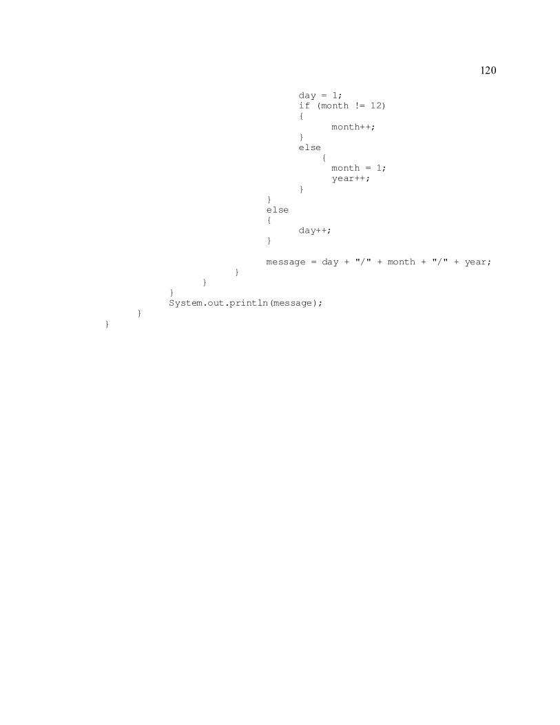
120
day = 1;
if (month != 12)
{
month++;
}
else
{
month = 1;
year++;
}
}
else
{
day++;
}
message = day + "/" + month + "/" + year;
}
}
}
System.out.println(message);
}
}
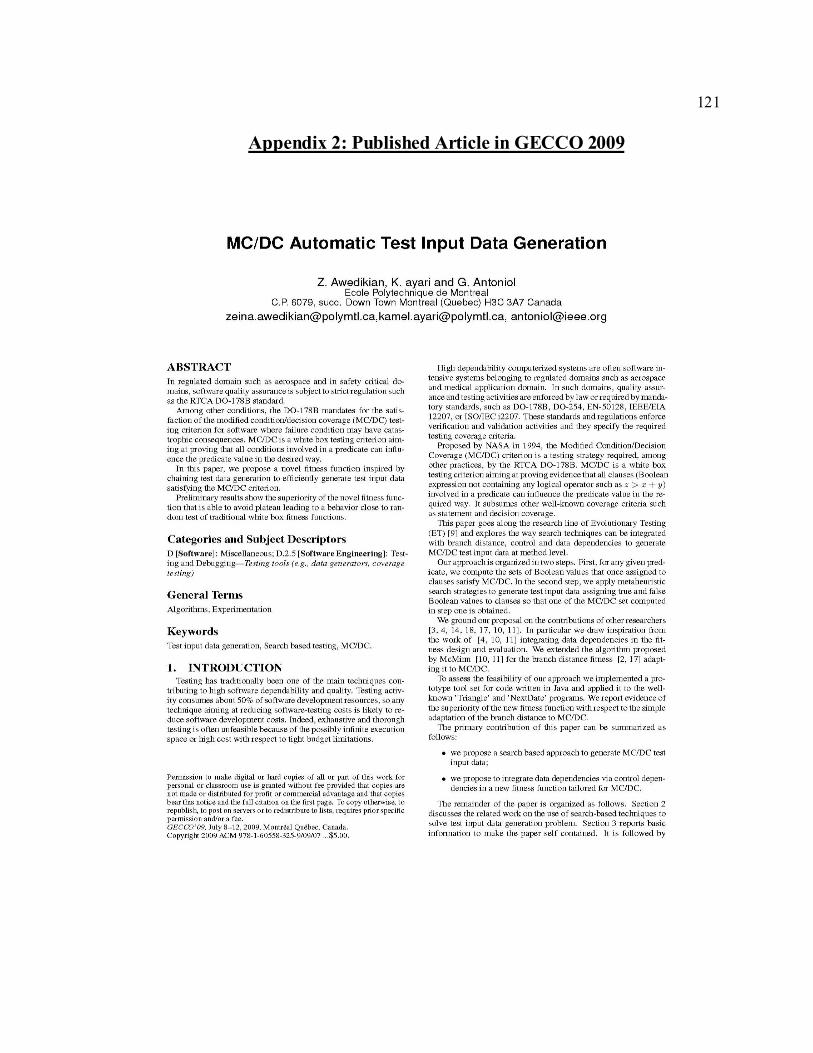
121
Appendix 2: Published Article in GECCO 2009
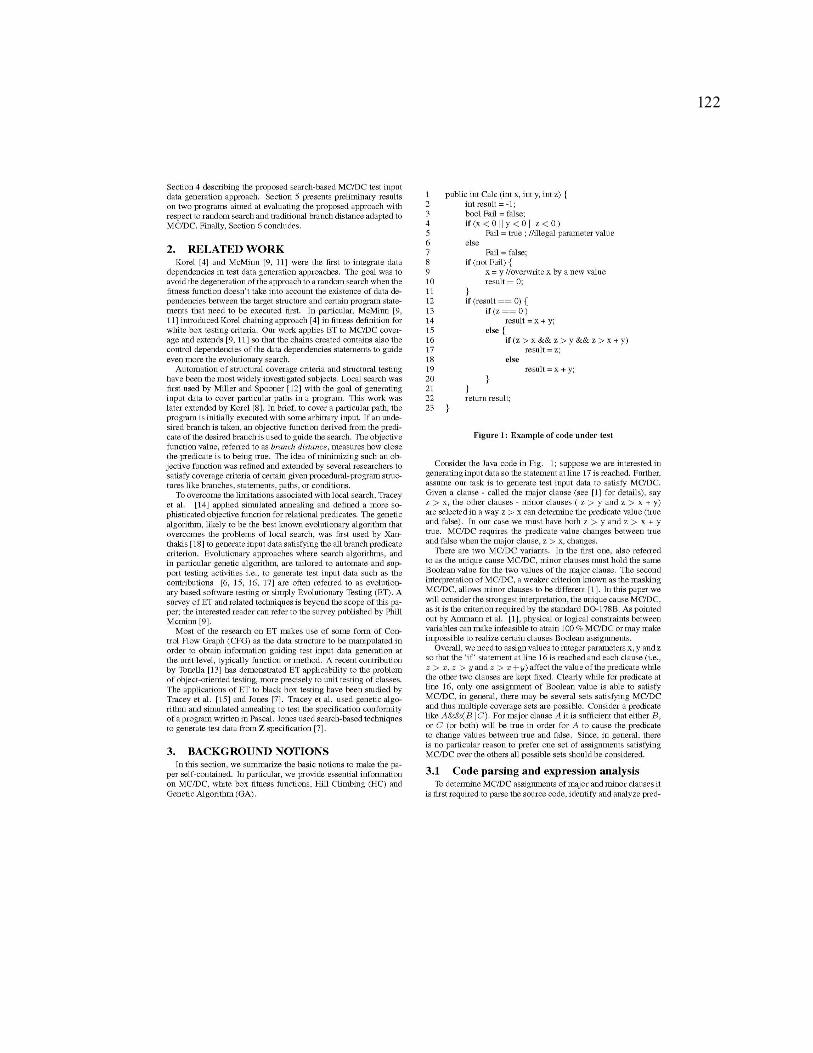
122

123

124

125

126

127

128