Embed Size (px)
Citation preview

CSE302 Automatic Control Engineering
Lecture 2: Mathematical Modeling of Control Systems
Asst. Prof. Dr.Ing.
Mohammed Nour A. [email protected]
https://mnourgwad.github.io
Copyright ©2018 Dr.Ing. Mohammed Nour AbdelgwadAhmed as part of the course work and learning material.All Rights Reserved.Where otherwise noted, this work is licensed under a Cre-ative Commons Attribution-NonCommercial-ShareAlike4.0 International License.
Zagazig University | Faculty of Engineering | Computer and Systems Engineering Department |Zagazig, Egypt

Lecture: 2
Mathematical Modeling of Control Systems
Mathematical Models
Differential Equation Model
Block Diagram Representation
Mohammed Ahmed (Asst. Prof. Dr.Ing.) Automatic Control Engineering 2 / 29

Mathematical Models
Mathematical Model
A set of mathematical equations (e.g., differential equations) that describes the input-outputbehavior of a system.
These models are useful for simulation, prediction/forecasting, design/performanceevaluation, and analysis and design of control systems.
Lumped vs. Distributed Systems
lumped system has a finite number of state variables
distributed system has an infinite number of state variables
state variables
a set of variables whose values at any moment completely characterize the system
Mohammed Ahmed (Asst. Prof. Dr.Ing.) Automatic Control Engineering 3 / 29

Mathematical Models
There are different types of lumped-parameter models. The mostly used:
Differential equation model (for linear and nonlinear systems)
Transfer function model (for linear time invariant systems)
State space model (for linear and nonlinear, SISO, and MIMO systems)
Model TypeSystem Type
Input-output
differential
equation
State equations
Transfer function
Nonlinear
Linear
Linear Time Invariant
Mohammed Ahmed (Asst. Prof. Dr.Ing.) Automatic Control Engineering 4 / 29

Differential Equation Model
a time domain mathematical model of control systems.
For linear systems, we can often represent the system dynamics through an nth orderordinary differential equation (ODE):
y (n)(t) + a1y(n−1)(t) + a2y
(n−2)(t) + · · ·+ an−1y(t) + any(t) =
b0u(m)(t) + b1u
(n−1)(t) + b2u(b − 2)(t) + · · ·+ bn−1u(t) + bmu(t)
Input: u(t); Output: y(t), system parameters: a1, · · · , an; b0, · · · , bm
The y (k) notation means we’re taking the k th derivative of y(t)
system order is the order of the ODE
Typically, m > n
Mohammed Ahmed (Asst. Prof. Dr.Ing.) Automatic Control Engineering 5 / 29

Differential Equation Model
Example
Derive the model of the following series RLC circuitwith input voltage applied to circuit vi and voltageacross the capacitor,vo as output.
Mesh equation: vi = Ri + L didt + vo
Substituting with capacitor current i = c dvodt
vi = RCdvodt
+ LCd2vodt2
+ vo ⇒d2vodt2
+
(
R
L
)
dvodt
+
(
1
LC
)
vo =
(
1
LC
)
vi
The above equation is a second order differential equation.
Mohammed Ahmed (Asst. Prof. Dr.Ing.) Automatic Control Engineering 6 / 29

Transfer Function
Transfer Function
the ratio of Laplace transform of output and Laplace transform of input by assuming all theinitial conditions are zero.
L{u(t)} = U(s), L{y(t)} = Y (s), L : is the Laplace operator
Transfer Function =L{y(t)}
L{x(t)}
∣
∣
∣
∣
IC=0
=Y (s)
X (s)
Given that ODE description, we can take the Laplace Transform:
H(s) =Y (s)
U(s)=
sm + bm−1sm−1 + · · ·+ b0
sn + an−1sn−1 + · · ·+ a0
denominator polynomial order > numerator polynomial order, transfer function is said tobe proper. Otherwise improper
Mohammed Ahmed (Asst. Prof. Dr.Ing.) Automatic Control Engineering 7 / 29
Transfer Function
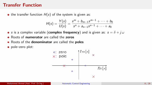
the transfer function H(s) of the system is given as:
H(s) =Y (s)
U(s)=
sm + bm−1sm−1 + · · ·+ b0
sn + an−1sn−1 + · · ·+ a0
s is a complex variable (complex frequency) and is given as: s = δ + j ω
Roots of numerator are called the zeros
Roots of the denominator are called the poles
pole–zero plot:
Mohammed Ahmed (Asst. Prof. Dr.Ing.) Automatic Control Engineering 8 / 29

Transfer FunctionExample
Given: H(s) =2s + 1
s3 − 4s2 + 6s − 4Zeros: z1 = -0.5
Poles: solve s3 -4s2 +6s -4 = 0,
use MATLAB roots command:
1 > poles = roots [1 -4 6 -4]
2 poles =
3 2,
4 1 + j, 1 - j
Factored form:
H(s) =2s + 0.5
(s − 2)(s − 1− j)(s − 1 + j)
Mohammed Ahmed (Asst. Prof. Dr.Ing.) Automatic Control Engineering 9 / 29

Analyzing Generic Physical Systems
Seven-step algorithm:
1 Identify dynamic variables, inputs (u), and system outputs (y)2 Focus on one component, analyze the dynamics (physics) of this component
◮ How? Use Newton’s Equations, KVL, or thermodynamics laws, etc.
3 After that, obtain an nth order ODE:
n∑
i=1
αi y(i)(t) =
m∑
j=1
βj u(j)(t)
4 Take the Laplace transform of that ODE
5 Combine the equations to eliminate internal variables
6 Write the transfer function from input to output
7 For a certain control U(s), find Y (s), then y(t) = L −1{Y (s)}
Mohammed Ahmed (Asst. Prof. Dr.Ing.) Automatic Control Engineering 10 / 29
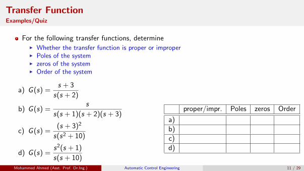
Transfer FunctionExamples/Quiz
For the following transfer functions, determine◮ Whether the transfer function is proper or improper◮ Poles of the system◮ zeros of the system◮ Order of the system
G (s) =s + 3
s(s + 2)a)
G (s) =s
s(s + 1)(s + 2)(s + 3)b)
G (s) =(s + 3)2
s(s2 + 10)c)
G (s) =s2(s + 1)
s(s + 10)d)
proper/impr. Poles zeros Order
a)
b)
c)
d)
Mohammed Ahmed (Asst. Prof. Dr.Ing.) Automatic Control Engineering 11 / 29

Block DiagramRepresentation of Control Systems
Mohammed Ahmed (Asst. Prof. Dr.Ing.) Automatic Control Engineering 12 / 29

Introduction
Block Diagram
a shorthand pictorial representation of the cause-and-effect relationship of a system.
the block usually contains a description of or the name of the element, gain, or thesymbol for the mathematical operation to be performed on the input to yield the output.The arrows represent the direction of information or signal flow.
Mohammed Ahmed (Asst. Prof. Dr.Ing.) Automatic Control Engineering 13 / 29

Examples of Block DiagramsTemperature Control System
Mohammed Ahmed (Asst. Prof. Dr.Ing.) Automatic Control Engineering 14 / 29

Importance of Block Diagrams
Graphical representation of interconnected systems are important
A system may consist of multiple subsystems: the output of one may be the input toanother, and so on
Each subsystem is represented by a functional block, labeled with the correspondingtransfer function
Blocks are connected by arrows to indicate signal flow directions
Advantages:
Easy for visualization purpose
Can represent a class of similar systems
Most importantly: can infer overall relationship between inputs and outputs, and henceanalyze the system stability and performance
Mohammed Ahmed (Asst. Prof. Dr.Ing.) Automatic Control Engineering 15 / 29

Block Diagram Building BlocksSumming Point
indicates the operations of addition and subtraction
represents by a circle (with or without X inside) with the appropriate plus or minus signassociated with arrows into the circle.
The output is the algebraic sum of the inputs.
Any number of inputs may enter a summing point.
Mohammed Ahmed (Asst. Prof. Dr.Ing.) Automatic Control Engineering 16 / 29

Block Diagram Building BlocksTakeoff Point
used for signal branching to have the same signal or variable as input to other blocks
This permits the signal to proceed unaltered along several different paths to severaldestinations.
Mohammed Ahmed (Asst. Prof. Dr.Ing.) Automatic Control Engineering 17 / 29

Block Diagram Building BlocksExample
Consider the following block diagram in which x1, x2, x3 , are variables, and a1, a2 aretransfer functions:
The output x3 is calculated as:x3 = a1 x1 + a2 x2 + 5
Mohammed Ahmed (Asst. Prof. Dr.Ing.) Automatic Control Engineering 18 / 29

Block Diagram Building BlocksExample/Quiz
Draw the Block Diagrams of the following equations.
x2 = a1dx1
dt+
1
b
∫
x1dt
x3 = a1d2x1
dt2+ 3
dx1
dt− bx1
Mohammed Ahmed (Asst. Prof. Dr.Ing.) Automatic Control Engineering 19 / 29
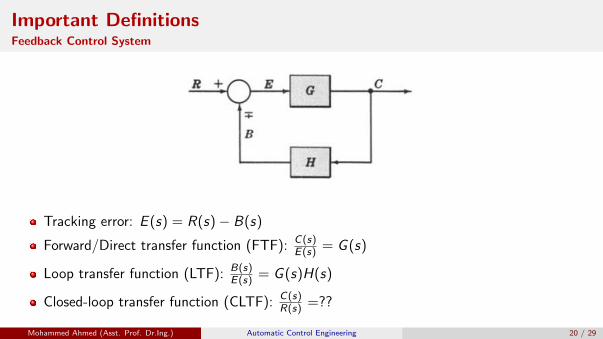
Important DefinitionsFeedback Control System
Tracking error: E (s) = R(s)− B(s)
Forward/Direct transfer function (FTF): C(s)E(s) = G (s)
Loop transfer function (LTF): B(s)E(s) = G (s)H(s)
Closed-loop transfer function (CLTF): C(s)R(s) =??
Mohammed Ahmed (Asst. Prof. Dr.Ing.) Automatic Control Engineering 20 / 29

Important DefinitionsCharacteristic Equation
The control ratio is the closed loop transfer function of the system.
The denominator of closed loop transfer function determines the system characteristicequation as:
C (s)
R(s)=
G (s)
1± G (s)H(s)
1± G (s)H(s) = 0
Mohammed Ahmed (Asst. Prof. Dr.Ing.) Automatic Control Engineering 21 / 29

Block Diagram AlgebraReduction techniques
Mohammed Ahmed (Asst. Prof. Dr.Ing.) Automatic Control Engineering 22 / 29

Block Diagram AlgebraReduction techniques
Mohammed Ahmed (Asst. Prof. Dr.Ing.) Automatic Control Engineering 23 / 29

Block Diagram AlgebraExamples
Find the CLTF utilizing the previous transformations
Hint: use property 4 (see previous slide)
Property 4: sliding a branch point past a function block
Mohammed Ahmed (Asst. Prof. Dr.Ing.) Automatic Control Engineering 24 / 29

Block Diagram AlgebraExamples
Mohammed Ahmed (Asst. Prof. Dr.Ing.) Automatic Control Engineering 25 / 29

Block Diagram AlgebraExamples
Can we use another property?
Yes, we can use Property 5 (moving a summing point ahead of a block)
Mohammed Ahmed (Asst. Prof. Dr.Ing.) Automatic Control Engineering 26 / 29

Block Diagram AlgebraExamples
Mohammed Ahmed (Asst. Prof. Dr.Ing.) Automatic Control Engineering 27 / 29

Block Diagram AlgebraExamples
Solution: First, let’s move H2 behind block G4 so that we can isolate theG3 − G4 − H1 feedback loop
Again, we use Property 4 to get:
Mohammed Ahmed (Asst. Prof. Dr.Ing.) Automatic Control Engineering 28 / 29
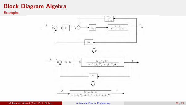
Block Diagram AlgebraExamples
Mohammed Ahmed (Asst. Prof. Dr.Ing.) Automatic Control Engineering 29 / 29

Thanks for your attention.
Questions?
Asst. Prof. Dr.Ing.
Mohammed Nour A. [email protected]
https://mnourgwad.github.ioRobotics Research Interest Group (zuR2IG)Zagazig University | Faculty of Engineering |
Computer and Systems Engineering Department| Zagazig, Egypt
Copyright ©2018 Dr.Ing. Mohammed Nour Abdelgwad Ahmed as part of the course work and learning material. All Rights Reserved.Where otherwise noted, this work is licensed under a Creative Commons Attribution-NonCommercial-ShareAlike 4.0 International License.
Mohammed Ahmed (Asst. Prof. Dr.Ing.) Automatic Control Engineering 30 / 29