Embed Size (px)
Citation preview

AC&ST
C. Melchiorri (DEI) Automatic Control & System Theory 1
AUTOMATIC CONTROL AND SYSTEM THEORY
SYSTEMS AND MODELS
Claudio Melchiorri
Dipartimento di Ingegneria dell’Energia Elettrica e dell’Informazione (DEI) Università di Bologna
Email: [email protected]

AC&ST
C. Melchiorri (DEI) Automatic Control & System Theory 2
Systems and Models
The terms: • “System” • “System theory” • “System engineering” • …
are frequently used in many –different– areas: process control, data elaboration, biology, economy, ecology, management, traffic control, … System: common “element” in this terminology Need of defining and analysing their structural properties

AC&ST
C. Melchiorri (DEI) Automatic Control & System Theory 3
Systems and Models
System: • A set, artificially isolated from the context, possibly made by more
(internal) interacting parts, • It is desired to study its “dynamic” behaviour
2
1 3
4
1 – 4: connections
External environment

AC&ST
C. Melchiorri (DEI) Automatic Control & System Theory 4
Systems and Models
• System: The time-evolution of a system is observable by means of a set of measurable attributes or variables that change in time
• Measurable attribute: Feature of the system that can be related to one or more integer, real or complex numbers, or in any case to a set of symbols
• Mathematical model: Expression by mathematical equations of the relationship between the measurable attributes
2
1 3
4

AC&ST
C. Melchiorri (DEI) Automatic Control & System Theory 5
Systems and Models
• The study of a system and of its properties is based on a mathematical model (although other models can be used as well) that describes, with a given approximation, the relationships among the system variables.
• Different models can be associated with a given system, and the chosen model depends on the desired representation level, precision, and complexity.
• The goal of the System Theory is to mathematically describe/represent a system in order to • understand its main physical properties and • design a proper control system.

AC&ST
C. Melchiorri (DEI) Automatic Control & System Theory 6
Systems and Models
• A system is graphically represented with a block, • Its variables are indicated by links to the external environment
or other systems.
S
S1 S2

AC&ST
C. Melchiorri (DEI) Automatic Control & System Theory 7
Systems and Models
• In an oriented system, it is possible to consider • Input variables (causes) • Output variables (effects)
• The separation between input and output variables is neither unique
nor clear
S
u1(t)
u2(t)
u3(t)
y(t)
input
output
Ra La c(t), ω(t)
Le va(t)
ia(t)
ve(t)
ie(t)

AC&ST
C. Melchiorri (DEI) Automatic Control & System Theory 8
Systems and Models
Distributed Parameters
Lumped Parameters
Stochastic Deterministic
Continuous time
Discrete time
Nonlinear Linear
Time Varying
Constant coefficients
Non homogeneous Homogeneous
Systems

AC&ST
C. Melchiorri (DEI) Automatic Control & System Theory 9
Systems and Models
Distributed Parameters
Lumped Parameters
Stochastic Deterministic
Continuous time
Discrete time
Nonlinear Linear
Time Varying
Constant coefficients
Non homogeneous Homogeneous
Systems

AC&ST
C. Melchiorri (DEI) Automatic Control & System Theory 10
Systems and Models: Static and Dynamic Systems
Two types of systems are considered: 1. Static systems (memory-less)
Mathematical model of static systems: • Algebraic equations – in a given instant, the output depends only
on the input value in that instant (e.g. the relation between the tension and the current in a resistance)
2. Dynamic systems (with memory) Mathematical model of dynamic systems (lumped parameters): • Differential equations – in a given instant, the output does not
depends only on the value of the input variables in that instant, but also on the previous values (e.g. the relation between the tension and the current in a capacitor)
Concept of state

AC&ST
C. Melchiorri (DEI) Automatic Control & System Theory 11
Lumped parameters models
• Physical properties are usually distributed in the systems: • Mass • Elasticity • Resistance • ...
• In their mathematical description, when possible it is better to introduce
approximations that allow to concentrate in one (or few) points those properties: Relevant simplifications can then be achieved in the mathematical descriptions.
• Lumped parameters models are obtained.
• In the practice, although it is evident that all the physical properties of systems are distributed, whenever possible it is advisable to use lumped parameter models.
Concentrated elasticity
Concentrated mass

AC&ST
C. Melchiorri (DEI) Automatic Control & System Theory 12
Lumped parameters models
Lumped parameters models are expressed by Ordinary Differential Equations, ODE, (continuous time) or Difference Equation (discrete time), that are function of time only:
When it is not possible to consider as concentrated (some of) the parameters of the system, it is necessary to use Partial Difference Equations, PDE. In this case, the dynamics is not only a function of time, but ALSO e.g. of space:

AC&ST
C. Melchiorri (DEI) Automatic Control & System Theory 13
Systems and Models
• Static system (algebraic)
• Dynamic system
i(t)
v(t) R
i(t)
v(t) R
C
0 50 100 150 200 250 300 0 10 20 30 40 50 60
Time (s)
V, I
0 0.5 1 1.5 2 0
0.2
0.4
0.6
0.8
1
q
v
v(t) = R i(t)
AC&ST
C. Melchiorri (DEI) Automatic Control & System Theory 14
Systems and Models – Static systems
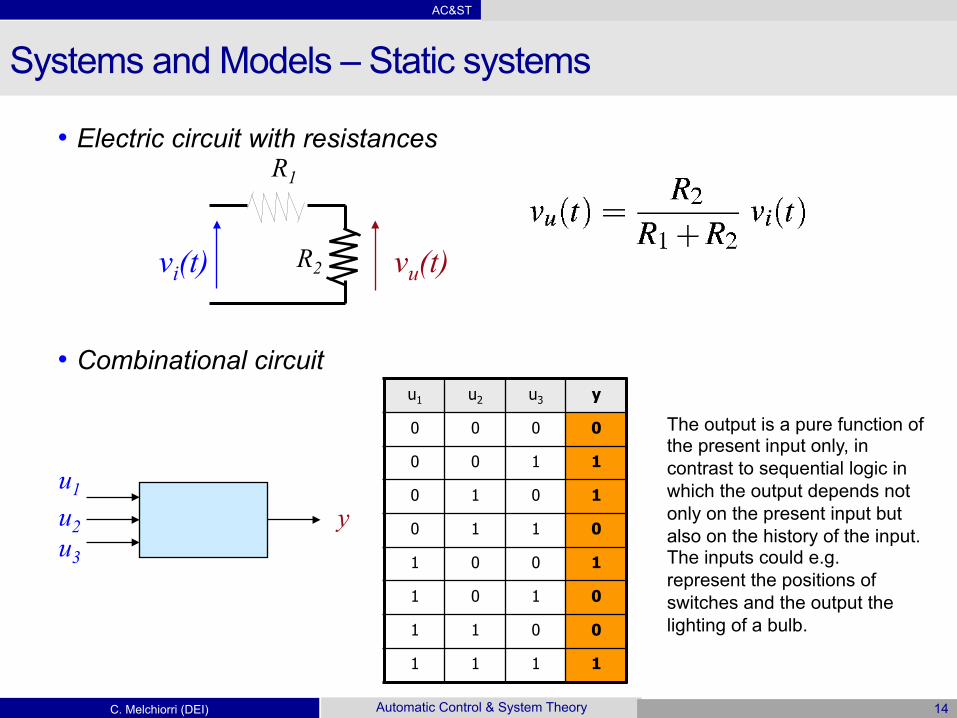
• Electric circuit with resistances
• Combinational circuit
vi(t)
R1
R2 vu(t)
u1
u2 u3
y
u1 u2 u3 y
0 0 0 0
0 0 1 1
0 1 0 1
0 1 1 0
1 0 0 1
1 0 1 0
1 1 0 0
1 1 1 1
The output is a pure function of the present input only, in contrast to sequential logic in which the output depends not only on the present input but also on the history of the input. The inputs could e.g. represent the positions of switches and the output the lighting of a bulb.
AC&ST
C. Melchiorri (DEI) Automatic Control & System Theory 15
Systems and Models – Dynamic systems
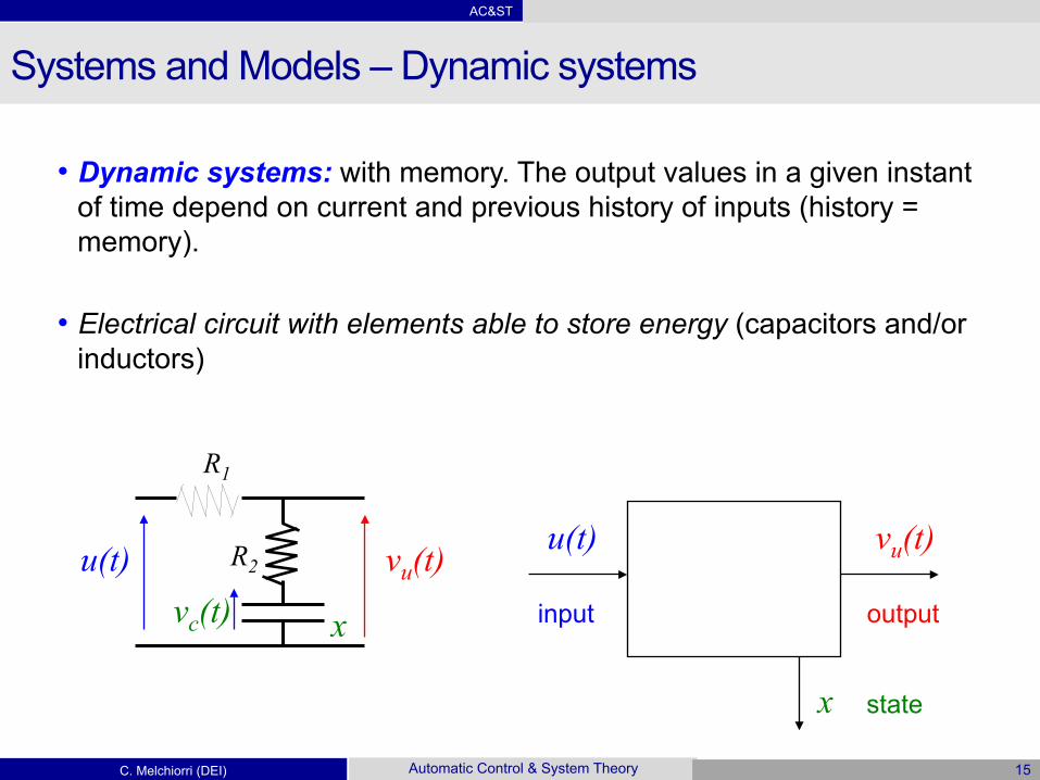
• Dynamic systems: with memory. The output values in a given instant of time depend on current and previous history of inputs (history = memory).
• Electrical circuit with elements able to store energy (capacitors and/or inductors)
R1
u(t) R2 vu(t) vc(t) x
u(t) vu(t)
x
input output
state

AC&ST
C. Melchiorri (DEI) Automatic Control & System Theory 16
Systems and Models – Dynamic systems
• Electrical circuit with elements able to store energy (capacitors and/or inductors)
• One obtains
R1
u(t) R2 vu(t) vc(t) x
u(t) vu(t)
x
input output
state

AC&ST
C. Melchiorri (DEI) Automatic Control & System Theory 17
Systems and Models
• The description of the system is made with two equations, a differential and an algebraic one:
u x y
State differential equation
Output equation

AC&ST
C. Melchiorri (DEI) Automatic Control & System Theory 18
Systems and Models
• The description of the system is made with two equations, a differential and an algebraic one:
• In general, it is difficult to solve the state differential equation. However, for a given class of systems (i.e. linear, continuous time, lumped systems) and given the initial state x(0) = x0 (value of the state at t = 0), one obtains:
State transition equation
State differential equation
Output equation
Similar equations hold also in the discrete time case.

AC&ST
C. Melchiorri (DEI) Automatic Control & System Theory 19
Systems and Models
• The equation valid also for the vector case, is the so-called Lagrange’s formula
• It is computed from the derivative of an integral (fundamental theorem of calculus)
with

AC&ST
C. Melchiorri (DEI) Automatic Control & System Theory 20
Systems and Models
Main analysis problems in System Theory are:
• Motion analysis – Output analysis: computation of the motion of the state (time evolution of x) or of the output function y(t), given the initial state x(0) = x0 and the input function u(t)
• Controllability analysis: how to affect the state motion or the output function acting on the input variable
• Observability analysis: computation of the state of the system in a given instant t, given the input and output values over the course of time period
• Sensitivity analysis: study of the influence on the state/output evolution of changes in the initial state, of the input function, of the system’s parameters
• Stability analysis: in a stable system, limited variations of the initial state or of the input function generate limited variations of the state evolution or of the output

AC&ST
C. Melchiorri (DEI) Automatic Control & System Theory 21
Systems and Models
Main synthesis problems in System Theory are:
• Input synthesis: definition of an input function that generates, given an initial state, a desired state evolution or a desired output function
• Synthesis of the input and of initial state: determination of an input function and of an initial state that generate a desired state evolution or a desired output function
• Control synthesis: design and implementation of a device that, properly connected to the system, allows achieving desired properties and behaviors in terms of stability, disturbance rejection, output properties, …

AC&ST
C. Melchiorri (DEI) Automatic Control & System Theory 22
Systems and Models
• Concept of state for a dynamic system The “state” is the information on the “internal condition” of a dynamic system that is needed in each instant in order to predict the effect of the previous history of the system itself on its future behavior
• In physical systems, the “internal condition” is typically determined by an
energy storage (also momentum or mass)
• It is advisable, in the definition of the state variables, to choose variables related to these storages (e.g. the voltage of a capacitor or of an inductor in an electrical circuit, the velocity of a mass in a mechanical system, …)
• The state variables and the state equations are NOT defined uniquely!

AC&ST
C. Melchiorri (DEI) Automatic Control & System Theory 23
Systems and Models
Considerations related to storage/transmission of energy In each physical domain of interest, excluding the thermal one, there are two “components” that are able to store energy:
• Electrical • Capacitor (C) and Inductor (L)
• Mechanical (linear) • Mass (M) and compliance (1/K)
• Mechanical (rotational) • Inertia (J) and rotational compliance (1/K)
• Fluid flow (hydraulic/pneumatic) • Fluid Capacitor (Cf) and Fluid Inductor (Lf)
• Thermal • Thermal Capacitor (Ct)

AC&ST
C. Melchiorri (DEI) Automatic Control & System Theory 24
Considerations related to storage/transmission of energy The two basic elements to store energy:
Systems and Models
Effort variables are computed as “differences”
Domain “capacitive” storage “inductive” storage
E Cv=12
2 E Li=12
2electrical
mechanical (linear) E Mv=
12
2 EKf=
121 2
mechanical (rotational)
E J=12
2ω EKc=
121 2
hydraulic/pneumatic E C pf=12
2 E L qf=12
2
thermic E C Tt= Non present
Flow variables Effort variables The stored energy depends on the

AC&ST
C. Melchiorri (DEI) Automatic Control & System Theory 25
Systems and Models
Definition • The state of a dynamic system Σ:
• Is an element of the state set X • It may change in time,
• The state x(t0) at the instant t0, together with the segment of the input function u|[t0,t1], uniquely defines the output function y|[t0,t1]

AC&ST
C. Melchiorri (DEI) Automatic Control & System Theory 26
Systems and Models - Examples
• RLC circuit
Choice of the state variables Quantities related to energy storage:
i vc
R
vu(t)
L
C vi(t) i

AC&ST
C. Melchiorri (DEI) Automatic Control & System Theory 27
Systems and Models - Examples
R
vu(t)
L
C vi(t) i
2 states 1 output
• RLC circuit

AC&ST
C. Melchiorri (DEI) Automatic Control & System Theory 28
Systems and Models - Examples
• Electric circuit with more loops
R1 R2
R3 C2
C1
vi(t) vu(t) v2
v1
i1 i2 i3
i5
i4

AC&ST
C. Melchiorri (DEI) Automatic Control & System Theory 29
Systems and Models - Examples
• Electric circuit with more loops
R1 R2
R3 C2
C1
vi(t) vu(t) v2
v1
i1 i2 i3
i5
i4
2 states 1 output

AC&ST
C. Melchiorri (DEI) Automatic Control & System Theory 30
Systems and Models - Examples
Output discontinuity due to the presence of the term D in the output equation
0 0.5 1 1.5 2 -0.8 -0.6 -0.4 -0.2
0 0.2 0.4 0.6 0.8
1 1.2 States x1 and x2
0 0.5 1 1.5 2 -0.8 -0.6 -0.4 -0.2
0 0.2 0.4 0.6 0.8
1 1.2 Input and output
• Electric circuit with more loops
R1 R2
R3 C2
C1
vi(t) vu(t) v2
v1
i1 i2 i3
i5
i4
The time-evolution of the state is a continuous function!
AC&ST
C. Melchiorri (DEI) Automatic Control & System Theory 31
Systems and Models - Examples
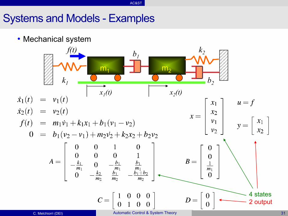
• Mechanical system f(t) k2
m1
x1(t)
m2
x2(t) k1
b1
b2
4 states 2 output

AC&ST
C. Melchiorri (DEI) Automatic Control & System Theory 32
Systems and Models - Examples
0 5 10 15 20 25 30 35 40 45 50 -1
-0.5
0
0.5
1
1.5
2
Tempo
Position of the two masses
x1
x2
f
m1 = 10; m2 = 5; k1 = 100; k2 = 50;
b1 = 10; b2 = 20;
0 10 20 30 40 50 -1
-0.5
0
0.5
1
1.5
2
Tempo
Position of the two masses
x1
x2
f
b1 = 50; b2 = 20;
f = 100 N
f(t) k2
m1
x1(t)
m2
x2(t) k1
b1
b2
• Mechanical system

AC&ST
C. Melchiorri (DEI) Automatic Control & System Theory 33
Systems and Models - Examples
• DC electric motor
Ra La Cm(t), ω(t)
Le
va(t)
ia(t)
ve(t)
ie(t)
vc(t)
Cr(t)
u y
x
3 states 2 input 1 output
if ve = const
AC&ST
C. Melchiorri (DEI) Automatic Control & System Theory 34
Systems and Models - Examples
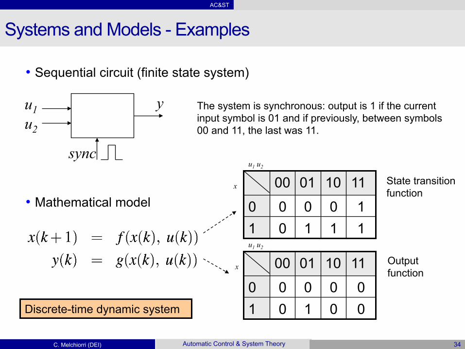
• Sequential circuit (finite state system)
• Mathematical model
u1
sync
y u2
The system is synchronous: output is 1 if the current input symbol is 01 and if previously, between symbols 00 and 11, the last was 11.
1 1 1 0 1 1 0 0 0 0
11 10 01 00
0 0 1 0 1 0 0 0 0 0
11 10 01 00
u1 u2
u1 u2
x
x
State transition function
Output function
Discrete-time dynamic system

AC&ST
C. Melchiorri (DEI) Automatic Control & System Theory 35
Systems and Models - Examples
• Another case of discrete time systems is obtained e.g. when a continuous time system is controlled by a digital computer: sampled data
u(k)
y(k) T
T
R1
u(t) R2 vu(t) vc(t) x

AC&ST
C. Melchiorri (DEI) Automatic Control & System Theory 36
Systems and Models - Examples
• Another case of discrete time systems is obtained e.g. when a continuous time system is controlled by a digital computer: sampled data
R1
u(t) R2 vu(t) vc(t) x
u
t
u(0) u(1)
u(2)
u(3) u(4)
0 T 2T 3T 4T
• If the input is a piecewise constant signal, and if the output is sampled at the same instants of time kT in which the input changes, then:

AC&ST
C. Melchiorri (DEI) Automatic Control & System Theory 37
Systems and Models - Examples
• The state transition function in this case is given by
AC&ST
C. Melchiorri (DEI) Automatic Control & System Theory 38
Systems and Models - Definitions
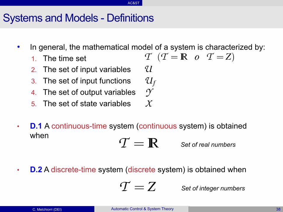
• In general, the mathematical model of a system is characterized by: 1. The time set 2. The set of input variables 3. The set of input functions 4. The set of output variables 5. The set of state variables
• D.1 A continuous-time system (continuous system) is obtained when
• D.2 A discrete-time system (discrete system) is obtained when
Set of real numbers
Set of integer numbers

AC&ST
C. Melchiorri (DEI) Automatic Control & System Theory 39
Systems and Models - Definitions
Definition:
• A model (system) is causal (nonanticipative or physical) when the output depends only on past and current values of the input
• A non-causal model (system) is called anticipative or acausal.
• An anticipative model does not correspond to any physical system • It is not conceivable a system reacting to an input before it is applied.

AC&ST
C. Melchiorri (DEI) Automatic Control & System Theory 40
Systems and Models - Definitions
is not causal if x is the input and y is the output of the system. The derivative function is defined as ⇒ it is necessary to know the future value of the function!
It is not possible to implement an ideal derivative function
The model
The model is causal if y is the input and x the output
Non causal models are used sometimes for analysis and algebraic manipulation purposes.
y(t) = a d x(t)d t

AC&ST
C. Melchiorri (DEI) Automatic Control & System Theory 41
Causal systems and models
• Example (non physical system):
• The amplitude (then the energy) of the output signal y(t) would increase (to infinite) if
the frequency ω of the input is increased!
0 2 4 6 8 10 -4 -2 0 2 4 A = 1, ω = 2 rad/sec
0 2 4 6 8 10 -4 -2 0 2 4 A = 1, ω = 4 rad/sec
Tempo (sec)
x(t) y(t)
limh!0
x(t+ h)! x(t)
h
d x(t)
d t
1
x(t) = A sinωt
y(t) =d x(t)
d t= A ω cosωt

AC&ST
C. Melchiorri (DEI) Automatic Control & System Theory 42
Systems and Models - Definitions
• D.3 A system is called memory-less (or purely algebraic) if it is composed by the sets and by an input/output function
• D.4 A system is called continuous-time dynamic system if it is composed by the sets , by a state differential equation
which admits a unique solution for each initial state and for each admissible input function, and by an output function

AC&ST
C. Melchiorri (DEI) Automatic Control & System Theory 43
Systems and Models - Definitions
• D.5 A system is called discrete-time dynamic system if it is composed by the sets , by a future state equation
and by an output function • D.6 A system is purely dynamic if its output function is
expressed as
i.e. it does not depend directly on the input

AC&ST
C. Melchiorri (DEI) Automatic Control & System Theory 44
Systems and Models - Definitions
u z
y
Purely dynamic system
Purely algebraic system
Non present in purely dynamic systems
n Separation principle: dynamic part (with state) algebraic part
n D.7 A system is called time-invariant or stationary if the time variable does not appear explicitly in the equations of its mathematical model. Otherwise, it is called non-stationary or time-varying.

AC&ST
C. Melchiorri (DEI) Automatic Control & System Theory 45
Time invariant models
• If the properties of a system do not depend on the time (i.e. they are time invariant), then the corresponding parameters are constant. The models of these systems are called stationary or time-invariant.
• In these cases, experiments are repeatable: the output obtained by applying a given input at time t0 with a given initial state x0 is the same (except a translation in time) obtained by applying, with the same initial state x0, the same input at time t0-δ.
0 0.5 1 1.5 2 2.5 3 3.5 4-1.5
-1
-0.5
0
0.5
1
1.5
2
2.5
Tempo (s)
x, y
0 0.5 1 1.5 2 2.5 3 3.5 4-1.5
-1
-0.5
0
0.5
1
1.5
2
2.5
Tempo (s)
x, y

AC&ST
C. Melchiorri (DEI) Automatic Control & System Theory 46
Time invariant models • From a practical point of view, usually the parameters of physical
systems change in time!
• On the other hand, it is sufficient that they do not change in a significant manner in a time period comparable with the `experiment’ duration.
• In time-invariant models, the initial time t0 is not important, and therefore the value t0 = 0 is usually considered.

AC&ST
C. Melchiorri (DEI) Automatic Control & System Theory 47
Systems and Models - Definitions
• D.8 A system is linear if 1. The sets U, Uf , X, and Y are vector space (defined on the
same field T ) 2. The functions defining its mathematical model are linear in x, u
for all the admissible t. Otherwise, a system is non-linear.
Commonly, a system is defined in mathematical term by:
Linear systems Non linear systems

AC&ST
C. Melchiorri (DEI) Automatic Control & System Theory 48
Systems and Models - Definitions
Purely algebraic system
Continuous-time dynamic system
Discrete-time dynamic system

AC&ST
C. Melchiorri (DEI) Automatic Control & System Theory 49
Systems and Models - Definitions
In order to take into account the physical limitation of the variables, the input set U is often considered limited
Examples:
• Input voltage for an electric motor -Va < v < Va
• Input flow in a tank 0 < u < U • …
u1
u2

AC&ST
C. Melchiorri (DEI) Automatic Control & System Theory 50
Systems and Models - Definitions
Classification of the systems on basis of the state
D.9 It is then possible to define: • Finite-State systems (state set: finite set)
• Finite-Dimensional systems (state set: finite-dimensional vector space)
• Infinite-Dimensional systems (state set: infinite-dimensional vector space)
= set of the states
Finite set
Vector space with Finite dimension
Infinite dimension
AC&ST
C. Melchiorri (DEI) Automatic Control & System Theory 51
Systems and Models - Definitions
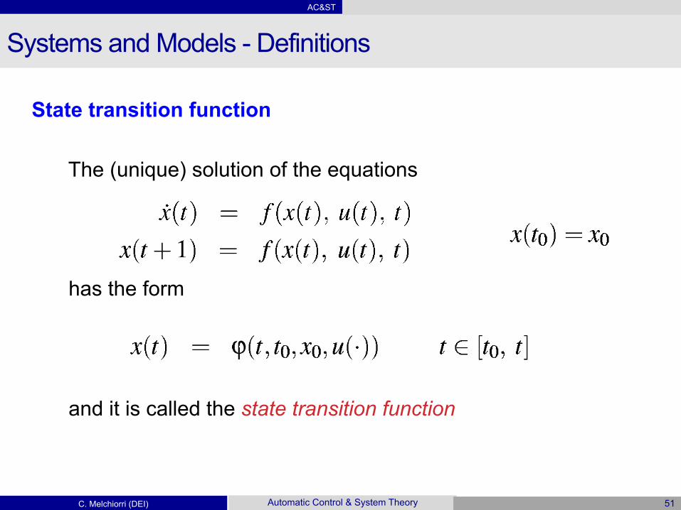
State transition function
The (unique) solution of the equations has the form
and it is called the state transition function

AC&ST
C. Melchiorri (DEI) Automatic Control & System Theory 52
Systems and Models - Definitions
Properties of the state transition function 1) Time orientation: it is defined for t ≥ t0, but not necessarily for t < t0
2) Causality: its dependence on the input function is restricted to the time interval [t0, t]:
ϕ(t, t0, x0, u1(.)) = ϕ(t, t0, x0, u2(.)) if u1|[t0,t] = u2|[t0,t]
3) Consistency: x = ϕ (t, t, x, u(.))
4) Composition: consecutive state transitions are congruent. i.e.,
ϕ(t, t0, x0, u(.)) = ϕ(t, t1, x1, u(.)) provided that
x1 = ϕ(t1 , t0 , x0 , u(.)) t0 ≤ t ≤ t1

AC&ST
C. Melchiorri (DEI) Automatic Control & System Theory 53
Systems and Models - Definitions
The last property (composition) means that
AC&ST
C. Melchiorri (DEI) Automatic Control & System Theory 54
Systems and Models - Definitions
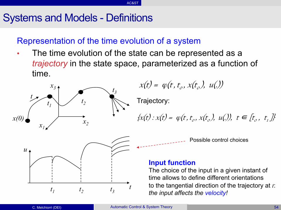
Representation of the time evolution of a system • The time evolution of the state can be represented as a
trajectory in the state space, parameterized as a function of time.
x2 x1
x3
x(0)
t t1
t2
t3
t
u
t1 t2 t3
Trajectory: {x(t) : x(t) = ϕ(t , t0 , x(t0 ), u(.)), t ∈ [t0 , t1 ]}
Input function The choice of the input in a given instant of time allows to define different orientations to the tangential direction of the trajectory at t: the input affects the velocity!
Possible control choices
x(t) = ϕ(t , t0 , x(t0 ), u(.))

AC&ST
C. Melchiorri (DEI) Automatic Control & System Theory 55
Systems and Models - Definitions
• Event: pair {t, x(t)} ∈ T x X • Motion or Movement for t ∈ [t0, t1] is the set of events defined by the
transition function
The motion is defined in the space T x X
• Trajectory: image in X of the transition function for t ∈ [t0, t1]
The trajectory is defined in X
0 2 4 6 8 10
0 1
2 3 0
0.5 1
1.5 2
t x1"
x 2"
Trajectory
Motion

AC&ST
C. Melchiorri (DEI) Automatic Control & System Theory 56
Systems and Models - Definitions
• For any given initial state, different input functions cause different trajectories, all initiating at the same point of the state space;
• Selecting input at a particular instant of time (for instance, t3) allows different orientations in space of the tangent to the trajectory at t3, namely of the state velocity
x2 x1
x3
x(0)
t t1
t2
t3
t
u
t1 t2 t3
x1, x2, x3
AC&ST
C. Melchiorri (DEI) Automatic Control & System Theory 57
Systems and Models - Definitions
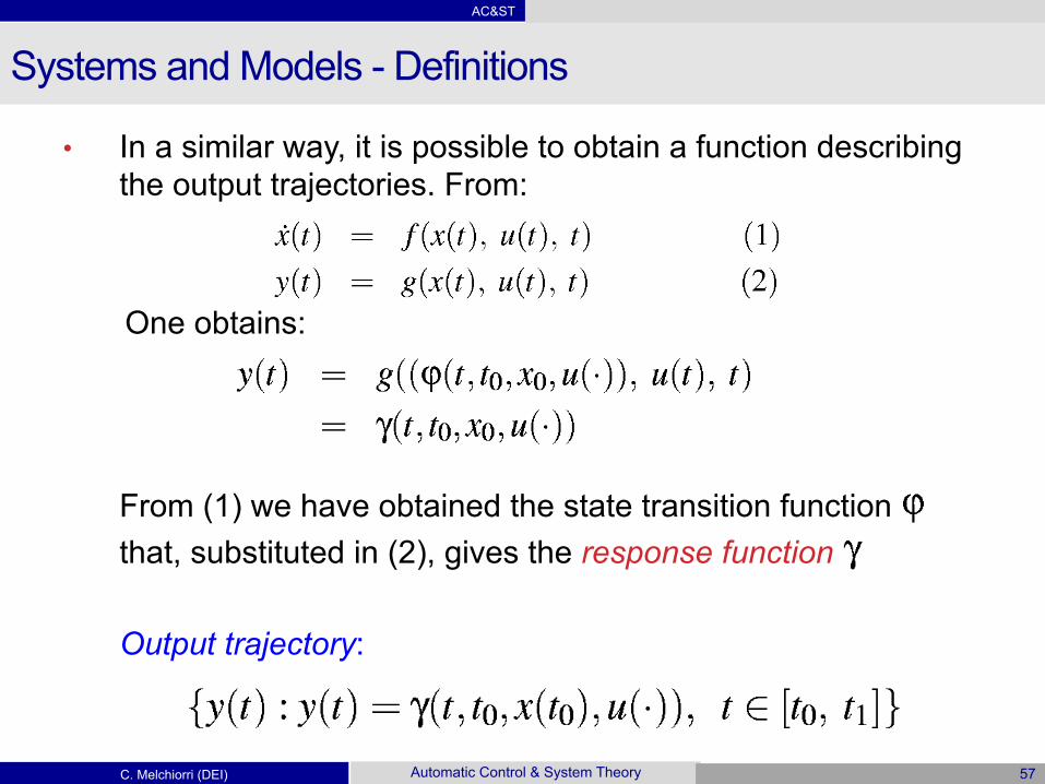
• In a similar way, it is possible to obtain a function describing the output trajectories. From:
One obtains:
From (1) we have obtained the state transition function that, substituted in (2), gives the response function
Output trajectory:

AC&ST
C. Melchiorri (DEI) Automatic Control & System Theory 58
Systems and Models - Definitions
In conclusion: • A system, once the differential equation of its
mathematical model has been solved, is characterized by a state transition function
• and by a response function

AC&ST
C. Melchiorri (DEI) Automatic Control & System Theory 59
Systems and Models - Definitions
• D.10 Indistinguishable states in [t0, t1] : the states x1 , x2 ∈ X are indistinguishable if
• D.11 Equivalent states: the states x1 , x2 ∈ X are equivalent if they are indistinguishable for each pair of instants
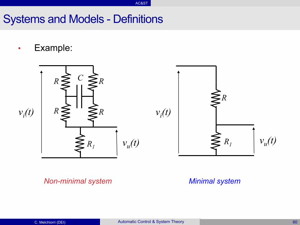
• D.12 Minimal system: is a dynamic system without equivalent states
A non-minimal system can be put in minimal form by defining a new state set in which each state corresponds to a class of equivalent old states.
AC&ST
C. Melchiorri (DEI) Automatic Control & System Theory 60
Systems and Models - Definitions
• Example:
vu(t)
vi(t)
R R
R R
R1
C
vu(t)
vi(t) R
R1
Non-minimal system Minimal system

AC&ST
C. Melchiorri (DEI) Automatic Control & System Theory 61
Systems and Models - Definitions
• Example:
θ(t), ω(t) va(t)
cr(t)
q(t)
z
Motor
Pump
Pump: cr = kp ω, q = kq ω Tank: dz / dt = ks q
When the two models are considered together, two equivalent states are identified (θ, z). One of them can be ignored: in this case θ since we want to control the liquid level only.

AC&ST
C. Melchiorri (DEI) Automatic Control & System Theory 62
Systems and Models - Definitions
• D.13 Equivalent systems: the systems Σ1 and Σ2 are equivalent if they are compatible, i.e.
and if to any state x1 ∈ X (x2 ∈ X) of Σ1 it is possible to associate a state x2 ∈ X (x1 ∈ X) of Σ2 (and vice versa) such that
Σ1
Σ2
u(.)
x1
x2
y1
y2
limh!0
x(t+ h)" x(t)
h
d x(t)
d t
!(t, t0, x0, u1(·)) = !(t, t0, x0, u2(·)) if u1|[t0,t] = u2|[t0,t]
T1 = T2 = TU1 = U2 = UUf1 = Uf2 = Uf
Y1 = Y2 = Y
1

AC&ST
C. Melchiorri (DEI) Automatic Control & System Theory 63
Systems and Models - Definitions
• Example:
• The two systems are equivalent if
• The initial states must be such that
R1 vu(t)
L
vi(t) i0
R2
C
vi(t) vu(t) vc

AC&ST
C. Melchiorri (DEI) Automatic Control & System Theory 64
Systems and Models - Definitions
• As a matter of fact:
R1 vu(t)
L
vi(t) i0
R2
C vi(t) vu(t) vc
The two systems are equivalent if
The evolution of the states is such that
1
limh!0
x(t+ h)! x(t)
h
d x(t)
d t
!(t, t0, x0, u1(·)) = !(t, t0, x0, u2(·)) if u1|[t0,t] = u2|[t0,t]
T1 = T2 = TU1 = U2 = UUf1 = Uf2 = Uf
Y1 = Y2 = Y
!
x1 = !R1
Lx1 + 1
Lu
y = R1x1
!
x2 = ! 1CR2
x2 + 1CR2
u
y = x2
1
limh!0
x(t+ h)! x(t)
h
d x(t)
d t
!(t, t0, x0, u1(·)) = !(t, t0, x0, u2(·)) if u1|[t0,t] = u2|[t0,t]
T1 = T2 = TU1 = U2 = UUf1 = Uf2 = Uf
Y1 = Y2 = Y
!
x1 = !R1
Lx1 + 1
Lu
y = R1x1
!
x2 = ! 1CR2
x2 + 1CR2
u
y = x2

AC&ST
C. Melchiorri (DEI) Automatic Control & System Theory 65
Systems and Models - Definitions
• D.14 Temporary equilibrium state. In a dynamic system Σ , a state is a temporary equilibrium state in [t0, t1] if there exists an input function
such that
Among all the possible motions, particular and important motions are those constant. The corresponding trajectory results in a unique state, called equilibrium state.
f
m
s
s0
input
M = M0 + m t Mass 0 ≤ f ≤ F Force
Notice: equilibrium depends on the input!!

AC&ST
C. Melchiorri (DEI) Automatic Control & System Theory 66
Systems and Models - Definitions
• D.15 Equilibrium state: it is a temporary equilibrium state in [t0, t1] for any pair t0, t1 in T
• Example:
f s
s0
input
M = M0 Mass 0 ≤ f ≤ F Force
N.B. It may happen that not all the states s can be equilibrium states, because f is limited

AC&ST
C. Melchiorri (DEI) Automatic Control & System Theory 67
Systems and Models - Definitions
• Mathematical models:
• Particular cases: stationary models, linear models, linear stationary models
Input-state-output Differential model
Input-state-output Difference model
Input-state-output Global model
External Global model

AC&ST
C. Melchiorri (DEI) Automatic Control & System Theory 68
Systems and Models - Definitions
Time invariant systems (time-shifting of causes and effects) Time invariant systems satisfy the time-shifting of causes and effects property.
In time-invariant systems, the transition function and the response function verify the following equations:
t τ 0
u(t) uΔ(t)
uΔ(t) = u(t-τ) Shifted input function
Assume that

AC&ST
C. Melchiorri (DEI) Automatic Control & System Theory 69
Systems and Models - Definitions
In particular, if τ = -t0, one otains
Therefore, for time invariant systems: 1. It is always possible to consider as initial istant of time t0 = 0 2. The transition and the response functions depend in a linear
fashion on the difference t - t0 , not on t and t0 separately

AC&ST
C. Melchiorri (DEI) Automatic Control & System Theory 70
Systems and Models - Definitions
Linear systems
• Functions ϕ and γ are linear with respect to initial state and input function
Let consider two scalars α and β, and
In the particular case α = β = 1, these equations correspond to the so-called property of superposition of the effects.

AC&ST
C. Melchiorri (DEI) Automatic Control & System Theory 71
Systems and Models - Definitions
• Important consequence: for linear systems, the property of decomposability of state transition and response functions holds.
• Moreover: 1. Indistinguishable states in [t0, t1] generate the same free
response in [t0, t1] 2. A Linear System is in minimal form iff for any initial instant of
time t0 no different states generate the same free response
Free motion Forced motion
Free response Forced response

AC&ST
C. Melchiorri (DEI) Automatic Control & System Theory 72
Systems and Models - Definitions
Controllability and Reachability The term controllability denotes the possibility of influencing the motion x(.) or the response y(.) of a dynamical system Σ by means of the input function (or control function) u(.)∈Uf . It might be required to steer a system from a state x0 to x1 or from an event (t0, x0) to (t1, x1): if this is possible, the system is said to be controllable from x0 to x1 or from (t0, x0) to (t1, x1). Equivalent statements: • “the state x0 (or the event (t0, x0)) is controllable to x1 (or to (t1, x1))” and • “the state x1 (or the event (t1, x1)) is reachable from x0 (or from (t0, x0))”
AC&ST
C. Melchiorri (DEI) Automatic Control & System Theory 73
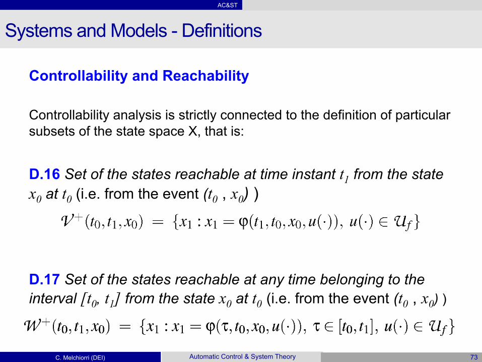
Systems and Models - Definitions
Controllability and Reachability Controllability analysis is strictly connected to the definition of particular subsets of the state space X, that is: D.16 Set of the states reachable at time instant t1 from the state x0 at t0 (i.e. from the event (t0 , x0) ) D.17 Set of the states reachable at any time belonging to the interval [t0, t1] from the state x0 at t0 (i.e. from the event (t0 , x0) )

AC&ST
C. Melchiorri (DEI) Automatic Control & System Theory 74
Systems and Models - Definitions
D.18 Set of the states controllable at the event (t1 , x1) from the initial time t0
D.19 Set of the states controllable at the event (t1 , x1) from any time in [t0, t1]
A property:

AC&ST
C. Melchiorri (DEI) Automatic Control & System Theory 75
Systems and Models - Definitions
Representation in X = R2 Set of the events (t, x)
t t0 t1
x(t1)
Events (t,x) corresponding to time t0, t1
x(t0)
Trajectory x(t) corresponding to [t0 t1]
x’(t0)
x”(t0) x’(t1)
x”(t1)

AC&ST
C. Melchiorri (DEI) Automatic Control & System Theory 76
Systems and Models - Definitions
t
These are the set of all the admissible motions with (t1, x1) or (t0, x0) as final or initial event.
t0 t1
x0
x1
Representation in X = R2 Set of the events (t, x)
Events (t,x) corresponding to time t0, t1

AC&ST
C. Melchiorri (DEI) Automatic Control & System Theory 77
Systems and Models - Definitions
Let’s define:
Then
Moreover:
Projection along t on P0 of
Projection along t on P1 of

AC&ST
C. Melchiorri (DEI) Automatic Control & System Theory 78
Systems and Models - Definitions
D.20 The state set of a dynamic system Σ or, by extension, system Σ itself, is said to be completely reachable from the event (t0, x) in the
time interval [t0, t1] if
D.21 The state set of a dynamic system Σ or, by extension, system Σ itself, is said to be completely controllable to the event (t1, x) in the time interval [t0, t1] if
t t0 t1 x
t t0 t1
AC&ST
C. Melchiorri (DEI) Automatic Control & System Theory 79
Systems and Models - Definitions
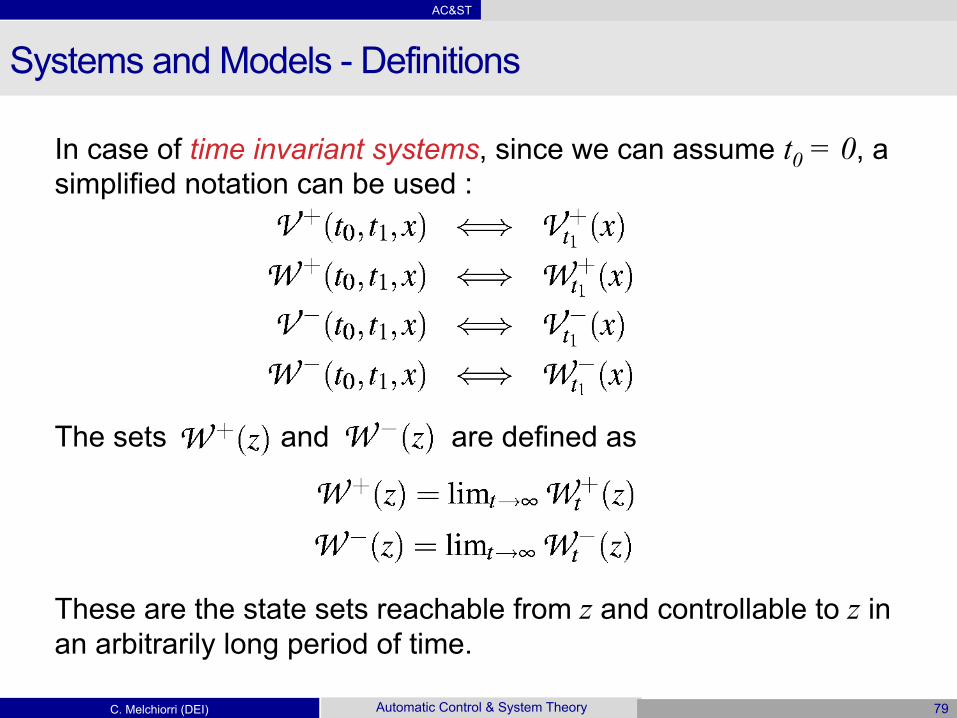
In case of time invariant systems, since we can assume t0 = 0, a simplified notation can be used :
The sets and are defined as These are the state sets reachable from z and controllable to z in an arbitrarily long period of time.

AC&ST
C. Melchiorri (DEI) Automatic Control & System Theory 80
Systems and Models - Definitions
• D.22 A time-invariant system is completely controllable (or connected) if it is possible to reach any state from any other state, so that W+(x)=W−(x)=X for all x∈X.
t t0 t1 x0
x1 x0

AC&ST
C. Melchiorri (DEI) Automatic Control & System Theory 81
Systems and Models - Definitions
Observability (and Reconstructability) The term observability denotes the possibility of deriving the initial state x(t0) or the final state x(t1) of a dynamic system Σ when the time evolutions of input and output in the time interval [t0, t1] are known. Final state observability is denoted also with the term reconstructability. The state observation and reconstruction problems may not always admit a solution: this happens, in particular, for observation when the initial state belongs to a class whose elements are indistinguishable in[t0, t1].

AC&ST
C. Melchiorri (DEI) Automatic Control & System Theory 82
Systems and Models - Definitions
Observability (and Reconstructability) Let’s define: • The set of all the initial states consistent with the functions u(.), y(.) in
the time interval [t0, t1]
• The set of all the final states consistent with the functions u(.), y(.) in the time interval [t0, t1]
where y(.) is not arbitrary, but constrained to the set of all the output functions admissible with respect to the initial state and the input function. This set is defined by

AC&ST
C. Melchiorri (DEI) Automatic Control & System Theory 83
Systems and Models - Definitions
The state set of a dynamic system Σ or, by extension, system Σ itself, is • Observable in [t0, t1] by a suitable experiment (called
diagnosis) if there exists at least one input function u(.)∈Uf such that reduces to a single element for all y(.) ∈ Yf (t0, u(.));
• Reconstructable in [t0, t1] by a suitable experiment (called homing) if there exists at least one input function u(.)∈ Uf such that reduces to a single element for all y(.)∈Yf (t0, u(.)).

AC&ST
C. Melchiorri (DEI) Automatic Control & System Theory 84
Systems and Models - Definitions
The state set of a dynamic system Σ or, by extension, system Σ itself, is • Fully observable in [t0, t1] if it is observable in [t0, t1] with any
input function u(.)∈Uf;
• Fully reconstructable in [t0, t1] ] if it is reconstructable in [t0, t1] with any input function u(.)∈Uf;

AC&ST
C. Melchiorri (DEI) Automatic Control & System Theory 85
Systems and Models - Definitions
• With time invariant system, we can adopt the notation
• Then:
Observable system
Reconstructable system
Fully reconstructable
system
Fully observable
system

AC&ST
C. Melchiorri (DEI) Automatic Control & System Theory 86
Systems and Models
The above sets are often considered in solving problems related to system control and observation. The most significant of these problems are:
1. Control between two given states: given two states x0 and x1 at two instants of time t0 and t1, where t1 > t0, determine an input function u(.) such that x1 =ϕ(t1, t0, x0, u(.)).
2. Control to a given output: given an initial state x0, an output value y1 at two instants of time t0, t1, where t1 > t0, determine an input u(.) such that y1 =γ(t1, t0, x0, u(.)).
3. Control for a given output function: given an initial state x0, an admissible output function y(.) at two instants of time t0, t1, where t1 > t0, determine an input u(.) such that y(t)=γ(t, t0, x0, u(.)) for all t∈[t0, t1].

AC&ST
C. Melchiorri (DEI) Automatic Control & System Theory 87
Systems and Models
4. State observation: given corresponding input and output functions u(.), y(-) at two instants of t0, t1, where t1 > t0, determine an initial state x0 (or the whole set of initial states) consistent with them, i.e., such that y(t)=γ(t, t0, x0, u(.)) for all t∈[t0, t1].
5. State reconstruction: given corresponding input and output functions u(.), y(.) at two instants of time t0, t1, where t1 > t0, determine a final state x1 (or the whole set of final states) consistent with them, i.e., corresponding to an initial state x0 such that x1 =ϕ(t1, t0, x0, u(.)), y(t)=γ(t, t0, x0, u(.)) for all t∈[t0, t1].
6. Diagnosis: like 4, except solution also includes the choice of a suitable input function.
7. Homing: like 5, except solution also includes the choice of a suitable input function.


