Automatic cartographic feature extraction has been Road ...code.eng.buffalo.edu/jrnl/Road_Estimation.pdf · Road Network Identification by means of the Hough Transform with Uncertainty

Road Network Identificationby means of the HoughTransform with UncertaintyAnalysis

ERIC SALERNONAGAVENKAT ADURTHITARUNRAJ SINGHPUNEET SINGLAADNAN BUBALOMARIA CORNACCHIAMARK ALFORDERIC JONES

The focus of this paper is on the use of ground target kinematics

to estimate the underlying road network on which the vehicles

are assumed to be travelling. Assuming that the road network

can be represented as an amalgamation of straight line segments,

a Hough transform approach is used to identify portion of road

which correspond to straight line segments. Since multiple tracks

can be associated with one segment of the road and since the

track estimates are inherently uncertain, an iterative approach

is presented to identify a parametric representation of the line

segments of the roads using the total least squares cost function.

Cramer-Rao bounds are identified to characterize the bounds on

the uncertainty associated with the proposed approach. A complex

dataset which include multiple tracks is used to illustrate the ability

of the proposed algorithm to identify the underlying road network

and characterize the uncertainty associated with the parametric

estimate of the road.

Manuscript received December 11, 2013; revised November 4, 2014and February 24, 2015; released for publication March 1, 2015.

Refereeing of this contribution was handled by Robert Lynch.

Authors’ addresses: E. Salerno, N. Adurthi, T. Singh, P. Singla,Dept. of Mech. & Aero. Eng., University of Buffalo, Buffalo,NY 14260 (e-mail: [email protected], [email protected], [email protected], [email protected]). A. Bubalo, M. Cornacchia,M. Alford, E. Jones, Information Directorate, Air Force Research Lab-oratory, Rome, NY 13441 (e-mail: [email protected]).

1557-6418/15/$17.00 c° 2015 JAIF

1 INTRODUCTION

Automatic cartographic feature extraction has beenthe goal for road network identification given thetremendous growth in automobiles with navigation sys-tems, and the interest in driverless cars. In post hurri-cane disaster scenarios when bridges and roads mightbe washed out, there is a need to rapidly update roadnetwork databases for logistics. In regions of conflict ordeserts, there is a need to develop road maps to iden-tify safe travel routes. Precise road networks can alsobe used to enhance the performance of ground vehicletrackers by restricting the motion of the target to theroad network.Synthetic Aperture Radar (SAR) and Ground Mov-

ing Target Indicator (GMTI) data is often processed andanalyzed to produce such networks. SAR produces im-ages of varying intensity which can be processed toseparate buildings, roads, and terrain. However, SARis only able to detect prominent existing features [1].For example, SAR will only detect a road if there is adistinct outline of such a path. GMTI on the other handtracks moving targets and relays the latitude and longi-tude coordinates as well as the kinematic information.The disadvantage of GMTI, however, is the necessity ofa moving target. Should the target stop or be obstructedin any way from the sensors, the tracker will lose thetarget for the duration of the obstructions [2]. Many ofthe currently available algorithms rely on informationfrom pre-existing road maps, however, in many scenar-ios the availability of this a priori information is limitedand inaccurate. In some situations there are no exist-ing road maps, such as in times of conflict in desertregions. Therefore the need for an algorithm which canaccurately estimate road networks in a timely manneris of great importance. Furthermore, there is a lack ofa real quantifiable measure of the accuracy of the ex-tracted road estimates. Several available algorithms usea “completeness” and “correctness” measure, which isa comparison of the extracted road network and the ac-tual network [3, 4, 5, 6]. However, as previously statedin many situations there are no available true networks(i.e., desert regions) so the metrics used to evaluate theperformance of algorithms are not relevant.Hu, Razdan, Femiani, Cui, and Wonka use a spoke

and wheel method in order to determine the foot-prints [5]. These footprints or polygons, are road seg-ments which span in any direction and terminate whenthe intensity of the spoke or line segment falls belowa threshold. Then a toe-finding algorithm is used todetermine the number of branches in the footprint. Inthis portion of the algorithm, if the angle between twobranches is less than 45 degrees they are merged, insome cases this will eliminate Y-shaped intersectionsand parallel roads. Instead of using centerlines to ap-proximate the road network they utilize inscribed linesto define the road structure. Finally the road network

58 JOURNAL OF ADVANCES IN INFORMATION FUSION VOL. 10, NO. 1 JUNE 2015

is trimmed to eliminate noisy data which might con-tribute to false roads, and also possible gaps betweenroads due to obstructions. This algorithm relies heavilyon pre-existing information pertaining to roads such asthe possible shapes of intersections, road widths, andangle of roads at these intersections.Tupin, Maitre, Mangin, Nicolas, and Pechersky first

identify linear features in the data and then separatethe true segments by using a Markov random field(MRF) [1]. Two different line detectors are used toidentify candidate road segments and then the resultsof these two detectors are fused together. With theidentification of the candidates, the MRF-based modelfills in large gaps and removes the false detections. ThisMRF-based model relies on a priori information of theroad network being developed. The assumption is madethat all roads lead to an initial starting point which canlimit the accuracy of the overall algorithm.Shackelford and Davis use a pixel-based fuzzy clas-

sifier and an object based classification approach toidentify the road networks [6]. Skeletonization is an ap-proach in which the image is thinned or eroded away un-til only the essential lines remain. This method producesa large amount of false positives in the road network.The second approach utilized is an iterative approachin which the longest roads are initially identified andthen shorter and shorter segments are added throughoutthe algorithm. The second algorithm proves to be muchbetter than skeletonization, however, the “completeness”measure of the road network has decreased in both theurban and suburban scenarios for the second algorithmwhen compared with the first.Sklarz, Novoselsky, and Dorfan focus on the fusion

of linear segments and curves based on a unified entityapproach rather than a single pixel based approach [7].The road network can either begin as a blank slate oralready contain roads. As new tracks become availablethe curve is associated with an existing curve if oneexists otherwise a new segment of road is added to theexisting network. Should a track already exist, the newtrack is cropped into segments to match with the rel-ative endpoints of the pre-existing road segments. Theoptimization of the curve fusion’s computational com-plexity increases drastically as the curves are discretizedinto more finite segments thus limiting the potential ofthe algorithm.Koch, Koller, and Ulmke utilize a Multiple Hypoth-

esis Tracking (MHT) algorithm, which consists of tar-get track extraction, prediction, filtering, track mainte-nance, and retrodiction [2]. It is assumed that the pos-terior probability density function is Gaussian, thus theKalman filter is utilized since the algorithm breaks theroad up into linear segments. The pruning removes anysegments, which have a weight smaller than a threshold,depending on the threshold this could cause some issueswith removing actual tracks. The merging depends onsegments having similar state vectors and covariances.

Fig. 1. Algorithm flow chart.

In this paper, a method for developing road networksand characterizing the uncertainty in these estimates isdeveloped. It is assumed that road networks can be bro-ken down into piecewise linear segments. Figure 1 il-lustrates the sequence of processing of data to generatea parameterization of the road network with the asso-ciated uncertainties. The initial processing of the datais done by creating a binary image of the track dataand extracting possible line segments using the Houghtransform. This is followed by the clustering of the dataassociated with the identified straight lines. Since theHough transform does not provide a measure of un-certainty, the Total Least Squares approach is imple-mented and the Cramer Rao lower bounds is derivedfrom this maximum likelihood estimate. The Total LeastSquares solution allows for an iterative estimate, whichis updated in time as additional measurements becomeavailable. The Least Squares solution will be used asan initial estimate for the recursive Total Least Squaresalgorithm. Once the data collection has been terminatedthe individual line segments can be merged, extendedor trimmed, and blended to produce a more completeroad network.Section 2 details the derivation of the Hough trans-

form for identifying straight line edges in an image.The recursive Total Least Squares solution is presentedin Section 3 along with the corresponding uncertaintyanalysis and derivations. In Section 4 the results of thealgorithms outlined are applied to a data set and weconclude the paper with suggestions for future researchin Section 5.

2 HOUGH TRANSFORM

The Hough transform is a well studied feature ex-traction technique that has been used extensively in

ROAD NETWORK IDENTIFICATION BY MEANS OF THE HOUGH TRANSFORM WITH UNCERTAINTY ANALYSIS 59

Fig. 2. Parameter identification.

image analysis [9]. This transform requires the imageto be binary in nature, where white pixels correspond toones and black pixels correspond to zeros. The deriva-tion of the Hough transform requires basic trigonomet-ric identities. Suppose we have a line oriented as shownin Figure 2 then by defining the parameters ½ andwe can derive the Hough transform. The perpendiculardistance from the origin to a line is denoted by ½. Theangle that this distance vector makes with the x-axis is .We note the definitions of the cosine and sine functions:

cos =x

½sin =

y

½: (1)

Algebraic substitution of a single cosine and sine termin the Pythagorean trigonometric identity leads to theequation:

x

½cos +

y

½sin = 1: (2)

It is now a simple matter to rearrange Equation (2) toobtain the conventional form of the Hough transform asgiven by the equation:

½= xcos + y sin : (3)

Now if Equation (3) is rearranged into a slope-intercept form

y =¡cossin

x+½

sin(4)

we can infer that when approaches zero degrees,corresponding to a vertical line, the slope tends to

Fig. 3. Collinear points.

infinity, resulting in an poor parameterization of the line.However, using Equation (3), we avoid this problem.The principle concept of the Hough transform in the

line identification algorithm can be stated as the follow-ing: if two points are collinear then they share a pair(½, ) of commonality in the Hough space. However, inorder to determine this common pair, a Hough matrixmust be constructed, this is done by iterating over arange of ¡90 to 90 degrees for each white pixel, whichcorresponds to the (x,y) coordinates, in the image. Re-call that is the angle the ½ vector makes with the x-axis.We can imagine that an arbitrary number of lines (blacksolid lines) pass through each coordinate shown by thesolid black lines in Figure 3, which are associated witha (½, ) given by the normal lines passing through theorigin shown by the dashed lines. The solid blue lineis the line of interest and Figure 3 illustrates two pointswhich lie on this line. Note that both these points illus-trated by the solid circle have a coincident (½, ) pair,which parameterize the dashed blue line.For each white pixel of the binary image with a

coordinate xi,yi determine the parameter

½( ) = xi cos( )+ yi sin( ) (5)

which corresponds to a sinusoid in the (½, ) space.Determine the (½, ) pair for every white pixel of thebinary images, round it to the closest discretized valueof (½, ), and augment the appropriate indices of anarray called the accumulator. Since every point on aline will share a unique (½, ) pair which correspondsto a line normal to the line of interest passing throughthe origin, the accumulator bin with the highest countwill correspond to parameters of a straight line. Figure 4illustrates the mapping of the Hough accumulator withthe white pixels indicating a higher count compared tothe black pixels. The point highlighted by the squarecorresponds to the (½, ) combination associated with astraight line.Matlab’s image processing toolbox is used to de-

termine the Hough transform, identify the peaks whichcorresponds to the straight lines, identify the points onthe images corresponding to the identified line segmentswhich are subsequently used to characterize the uncer-tainty of the identified lines.


Fig. 4. Hough transform.

3 MAXIMUM LIKELIHOOD ESTIMATORSIn this section we will derive the solutions for the

Total Least Squares (TLS) to estimate the parametersof a straight line. In this formulation, the measurementnoise covariance matrix is allowed to be populated, i.e.,the dependent and independent variables are noisy andcan be correlated. The Hough transform presented inSection 2 will be utilized to identify groups of nearlycollinear points in an image. A best fit line can beobtained using the TLS solution since there is noisein both the x and y directions. The TLS solution,which will be derived, does not have a closed formsolution and therefore requires an initial estimate toinitiate the solver which minimizes the normal distanceof the measurements from the line. This initial estimatecan be given by a transformed version of the Houghcoefficients (i.e., transform from ½ and to slope, mand intercept b), however if is zero degrees thenwe would obtain an infinite slope, which forces theTLS solution to diverge. Therefore, rather than usethe Hough transform coefficients transformed to theappropriate slope and intercept we will simply utilize aLeast Squares estimate as the initial guess for the TLSalgorithm.

3.1 Total Least SquaresConsider the problem of a straight line fit where the

true model is given by the equation:

yi =mxi+ c (6)

where yi and xi are the true dependent and indepen-dent coordinates. m and c correspond to the slope andordinate intercept of the line. Assuming that the mea-surement of both yi and xi are noisy, the measurementequations and the corresponding pdf of the noise aregiven by the equations:

xi = xi+ ºx (7)

yi = yi+ ºy (8)

p(º1,º2) =NÃ·º1

º2

¸:·0

0

¸,

"¾2xx ¾xy

¾xy ¾2yy

#!(9)

permitting the measurement noise in xi and yi to becorrelated. Note that ¾2xx and ¾

2yy denote the variance

of ºx and ºy respectively and ¾xy represent the cross-covariance of ºx and ºy. The notation N (º : ¹,§) is aGaussian probability density function(pdf) for the ran-dom vector º with mean ¹ and covariance §. Identifyingthe parameters of a line when provided with n measure-ments, the likelihood function for the measurements isgiven by the equation:

p=nYi=1

pi (10)

pi = p·xi

yi

¸jm,c,x1,x2, : : : ,xn

¶

=NÃ·xi¡ xiyi¡ yi

¸:·0

0

¸,

"¾2xx ¾xy

¾xy ¾2yy

#!(11)

=NÃ·

xi¡ xiyi¡mxi¡ c

¸:·0

0

¸,

"¾2xx ¾xy

¾xy ¾2yy

#!(12)

=NÃ·xi

yi

¸:·

xi

mxi+ c

¸,

"¾2xx ¾xy

¾xy ¾2yy

#!: (13)

The Log-Likelihood to be maximized with respect tothe free variables m, c and xi where i= 1,2, : : : ,n is

ln(p) =¡n ln³2¼q¾2xx¾

2yy ¡¾2xy

´¡ 12(¾2xx¾2yy ¡¾2xy)

nXi=1

(¾2yy(xi¡ xi)2

¡ 2¾xy(xi¡ xi)(yi¡mxi¡ c)+¾2xx(yi¡mxi¡ c)2): (14)

There are n+2 variables: m, c, and all the n abscissasxi. Differentiate the log-likelihood with respect to thevariables and solve the n+2 equations:

@ ln(p)@m

=¡ 12(¾2xx¾

2yy ¡¾2xy)

£nXi=1

(2¾xy(xi¡ xi)xi¡ 2¾2xx(yi¡mxi ¡ c)xi) = 0

(15)

@ ln(p)@c

=¡ 12(¾2xx¾

2yy ¡¾2xy)

£nXi=1

(2¾xy(xi¡ xi)¡ 2¾2xx(yi¡mxi ¡ c)) = 0

(16)


@ ln(p)@xi

=¡ 12(¾2xx¾

2yy ¡¾2xy)

£ (¡2¾2yy(xi ¡ xi) +2¾xy(yi¡mxi¡ c)+2¾xy(xi¡ xi)m¡ 2¾2xx(yi ¡mxi¡ c)m) = 0:

(17)

Solving for the xi from equation (17) leads to theequation:

xi =c(¡m¾2xx+¾xy)¡m¾xyxi+¾2yyxi+m¾2xxyi¡¾xyyi

¾2yy +¾2xxm2¡ 2¾xym:

(18)Substituting the expression for xi back into the log like-lihood function ln(p) of equation (14) and on simplifi-cation, the final cost function in terms of m and c is:

ln(p) =¡n ln³2¼q¾2xx¾

2yy ¡¾2xy

´¡ 12

nXi=1

(yi¡mxi¡ c)2¾2yy +¾2xxm2¡ 2¾xym

(19)

or the problem can be stated as

minm,c

nXi=1

(yi¡mxi¡ c)2¾2yy +¾2xxm2¡2¾xym

: (20)

Additionally, the noise covariance parameters can bespecific to each measurement, i.e., ¾xx,¾yy, and ¾xy canbe ¾(i)xx ,¾

(i)yy and ¾

(i)xy respectively corresponding to the

measurement (xi, yi). It can be observed that, when thenoise in the variables is uncorrelated (¾xy = 0) and ofequal variance(¾xx = ¾yy = ¾), the standard Total leastsquare problem is recovered, which can be identifiedas the perpendicular distance of (xi, yi) to the line y =mx+ c, and

minm,c

nXi=1

(yi¡mxi¡ c)21+m2

is the resulting cost function to be minimized.

3.2 Alternate Equivalent Formulation

The algebraic manipulation involved in arriving atthe cost function of (20) can be avoided altogether.Consider the truth model where we represent the truth(xi,yi) in terms of the noisy measurement (xi, yi) as:

yi =mxi+ c (21)

xi = xi¡ ºx (22)

yi = yi¡ ºy: (23)

Substituting (22) and (23) into (21) results in the equa-tion:

yi¡mxi¡ c= ºy ¡mºx: (24)

Define º 0 as:

º 0 =ºy ¡mºxq

¾2yy +¾2xxm2¡ 2m¾xy(25)

whose mean and variance of random variable º 0 condi-tioned on m are given by the equations:

E[º 0] = E

24 ºy ¡mºxq¾2yy +¾2xxm2¡ 2m¾xy

35=

E[ºy]¡mE[ºx]q¾2yy +¾2xxm2¡ 2m¾xy

= 0 (26)

E[º 02] = E

"(ºy ¡mºx)2

¾2yy +¾2xxm2¡ 2m¾xy

#

=E[º2y ] +m

2E[º2x ]¡ 2mE[ºxºy]¾2yy +¾2xxm2¡2m¾xy

= 1:

(27)

The random variable º 0 has a Gaussian distributiongiven by the equation:

p(º 0 jm) =N (º 0 : 0,1): (28)

But from equations (24) and (25), one has

º 0 =yi¡mxi¡ cq

¾2yy +¾2xxm2¡2m¾xy:

Hence, for a set of measurements (xi, yi), the MaximumLikelihood Estimator (MLE) requires maximizing thefunction given by Equation (10), which can be rewrit-ten as:

pi =N0@ yi¡mxi¡ cq

¾2yy +¾2xxm2¡ 2m¾xy: 0,1

1A : (29)

The negative of the Log-Likelihood to be minimizedwith respect to the free variables m and c is

J =¡ ln(p) =nXi=1

(yi¡mxi¡ c)2¾2yy +¾2xxm2¡2m¾xy

: (30)

Notice that there are no xi variables in the cost func-tion. Differentiating the cost function J only with thevariables m and c, we arrive at the gradient constraintequations:

@J

@m=

nXi=1

Ã2(yi¡mxi¡ c)(¡xi)¾2yy +¾2xxm2¡ 2m¾xy

¡ (yi¡mxi¡ c)2(2¾2xxm¡ 2¾xy)

(¾2yy +¾2xxm2¡ 2m¾xy)2!= 0

(31)

@J

@c=

nXi=1

(¡2(yi¡mxi¡ c)) = 0 (32)

which is nonlinear in m and c and can be solved nu-merically. One can use the solution of the least squaresproblem to initialize the nonlinear solver. One can also


estimate the most likely value of the variable xi usingthe equation:

xi =c(¡m¾2xx+¾xy)¡m¾xyxi+¾2yyxi+m¾2xxyi¡¾xyyi

¾2yy +¾2xxm2¡ 2¾xym(33)

from the resulting solution for the slope m and inter-cept c.

3.3 Geometric Interpretation

Consider the case of estimating the parameters ofa straight line where the xi and yi measurements arecontaminated by isotropic noise. Figure 5 illustrates thetrue xi and yi and the corresponding contaminated xiand yi data. Assuming the parameters ¾xx = ¾yy = 1 and¾xy=0, the MLE cost function given by Equation (30)reduces to:

J =nXi=1

(yi¡mxi¡ c)21+m2

(34)

which is referred to as geometric distance which is agradient weighted algebraic distance. This error referredto as the Sampson error is the first order approximationof the geometric distance of the point from the curve.In Figure 5, one can easily illustrate the line connect-

ing the points (xi, yi) along the normal to the true linehas a length given by equation (yi¡mxi¡ c)2=(1+m2),illustrating that the total least squares cost function cor-responds to minimizing the geometric distance. Notethat the least squares problem minimizes the distance(yi¡mxi¡ c)2 which is referred to as the algebraic dis-tance and corresponds to the distance along an obliqueprojection.

3.4 Least Squares

The least squares problem is a special case of thetotal least squares where the independent variable xi isnot random, i.e., ¾xx = 0. This results in the cost functiongiven by Equation (30) reducing to:

J =¡ ln(p) =nXi=1

(yi¡mxi¡ c)2¾2yy

(35)

which has a closed form solution for m and c:½m

c

¾=½Pn

i=1 x2i

Pni=1 xiPn

i=1 xi n

¾¡1½Pni=1 xiyiPni=1 yi

¾: (36)

3.5 Uncertainty Analysis

In this section, we will present the derivation for theCramer Rao lower bounds which provides a measureof uncertainty in the coefficients of the linear fit. Thederivation is based on a fully populated covariancematrix and the bounds are estimated by the inverseof the Fisher Information matrix. The derivations areaccompanied by a Monte Carlo simulation to verify theconvergence properties of the solutions. For the straight

Fig. 5. Total least squares minimization.

line we have a total of 2+n unknown parameters, theslope m, the intercept c, and the true values of x : xt.After solving for the optimal estimates for the slope

m and y-intercept c, the optimal estimate for xi is givenby Equation (33). Assuming the parameters ¾xx = ¾yy =1 and ¾xy=0, Equation (33) reduces to:

xi =¡cm+ xi+ myi

1+ m2(37)

) xi =¡cm+ xi+ xim2¡ xim2 + myi

1+ m2(38)

) xi = xi+mei1+ m2

(39)

whereei = yi¡ mxi¡ c (40)

is the error associated with the measurement yi and theestimate yi at the measured x coordinate xi. Figure 6illustrates the optimal estimates (xi, yi), which results inthe equation:

yi =yi¡ ei¡ m(xi¡ xi) (41)

yi =yi¡ei

1+ m2: (42)

It can be shown that the generalized solutions forthe estimated values for xti and yti are:

x2i = xi+(m¾2xixi ¡¾xiyi)ei

m2¾2xixi ¡ 2m¾xiyi +¾2yiyi(43)

y2i = yi+(m¾xiyi ¡¾2yiyi)ei

m2¾2xixi ¡ 2m¾xiyi +¾2yiyi(44)

based on Equation (33).Recall that ei is the error in the measurement with

the appropriate estimates ei =¡mxi¡ c+ yi. Note that in


Fig. 6. Optimal estimates of coordinates.

Equations (43) and (44), the estimate for the slope andintercept must be known in order to calculate x2i andy2i . In our scenario these initial estimates are given bythe basic Least Squares solution rather than the solutionof the Hough transform. This is to preclude singularestimates for the slope and intercept:

m=¡cossin

(45)

c=½

sin(46)

if the Hough transform returns a line estimate withexactly zero. Note that the Hough transform is used toidentify the measurements which are associated with theline which is being estimated.With the initial estimates for the slope and intercept,

one can update the estimate of the true value xi usingEquation (43). In addition to the estimated true valueof x, the line’s coefficients are updated using the TotalLeast Squares solution. The next step is to determine theuncertainty in these estimates. The probability densityfunction for (xi,yi), given the estimates [m, c, xi] is:

p(xi, yi j m, c, xi)

=1

2¼pjQij exp

"¡12

·yi

xi

¸¡·mxi+ c

xi

¸¶T£Q¡1i

·yi

xi

¸¡·mxi+ c

xi

¸¶¸:

(47)

The inverse of the covariance matrix Qi is easily definedfor a 2£ 2 matrix:

Q¡1i =1

¾2xi xi¾2yi yi¡¾2

xi yi

"¾2yi yi ¡¾xiyi¡¾xiyi ¾2xi xi

#: (48)

We expand the exponential term in Equation (47) andwrite it as a product of two variables ®i and Ki which

are defined in Equations (49) and (50), respectively:

®i =¡1

2(¾2xi xi¾2yi yi¡¾2

xi yi)

(49)

Ki = ¾2xi xi(yi¡ mxi¡ c)2¡ 2¾xiyi (yi¡ mxi¡ c)(xi¡ xi)

+¾2yi yi (xi¡ xi)2: (50)

With ®i and Ki defined for each measurement we canthen rewrite the likelihood function in a more contractedform as:

p(xi, yi j m, c, xi) =1

2¼pjQije®iKi : (51)

For each measurement, there is a corresponding (xi,yi),independent of one another. Therefore if we assumethere are a total of M measurements, the probabilitydensity function for the matrix of measurements, [x, y],given the parameter estimates, [m, c, x], where x is nowa vector of estimated x values, is given by the productof each measurement’s probability density function:

p(x, y j m, c, x) =MYi=1

1

2¼q(¾2xi xi¾2yi yi¡¾2

xi yi)e®iKi (52)

The Fisher Information matrix is defined as the nega-tive expected value of the Hessian of the log-likelihoodfunction with respect to the estimated parameters. Wedefine the log-likelihood function as, f = ln[p(x, y jm, c, x)], therefore the Fisher Information matrix is de-fined as:

F =¡E

266666664

@f

@m@m

@f

@m@c

@f

@m@x

¶T@f

@c@m

@f

@c@c

@f

@c@x

¶T@f

@x@m@f

@x@c@f

@x@x

377777775(53)

where

@f

@m@x=

@f

@x@m=·@f

@m@x1,@f

@m@x2, : : : ,

@f

@m@xM

¸Tand similarly @f=@c@x= @f=@x@c. The sub-block@f=@x@x of the Fisher Information matrix is a M £Mdiagonal matrix with diagonal elements:

@f

@x@x=Diag

·@f

@x1@x1,@f

@x2@x2, : : : ,

@f

@xM@xM

¸¶:

First the partial derivatives of f are taken with re-spect to the estimated parameters. Recall that the prob-ability density function is a product of the individualmeasurement’s and with the properties that the log of


the product becomes a summation over the M measure-ments. Thus the partial derivatives are:

@f

@m=

MXi=1

®i[¡2¾xiyi (¡xixi+ x2i )+¾2xi xi (¡2yix+i 2mx2i +2xic)] (54)

@f

@c=

MXi=1

®i[¡2¾xiyi (¡xi+ xi)+¾2xi xi (¡2yi+2mxi+2c)] (55)

@f

@xti= ®i[¾

2yi yi(¡2xi+2xi)

¡2¾xiyi (¡yi¡ xim+2mxi+ c)+¾2xi xi (¡2yim+2m2xi+2mc)]: (56)

Then the second derivatives, which compose the FisherInformation matrix, can easily be determined using theequations:

E

·@2f

@m@m

¸=

MXi=1

®i(2¾2xixix2i ) (57)

E

·@2f

@m@c

¸=

MXi=1

®i(2¾2xixixi) (58)

E

·@2f

@m@xti

¸= E

h®i(¡2¾xiyi (¡xi+2xi)+¾2xixi(¡2yi+4mxi+2c))

i= ®i(¡2¾xiyi xi+2¾2xixi mxi) (59)

E

·@2f

@c@c

¸=

MXi=1

2®i¾xixi (60)

E

·@2f

@xti@c

¸= ®i(¡2¾xiyi +2¾2xixi m),

i= 1,2, : : : ,M (61)

E

·@2f

@xti@xti

¸= ®i(2¾

2yiyi¡ 4¾xiyi m+2¾2xixi m2),

i= 1,2, : : : ,M (62)

E

"@2f

@xti@xtj

#= E

"@2f

@xtj @xti

#= 0, i 6= j: (63)

These equations then give us an estimate of the uncer-tainty in the estimated parameters. The next step is toperform a Monte Carlo simulation to show the conver-gence characteristics of this estimate. We begin the sim-ulation by choosing a slope, intercept, and range of xvalues. These will be the true simulation parameters andare specified as:

m=¡0:4326 c=¡1:6656 x=¡3 : 0:1 : 3: (64)

Fig. 7. Truth, measurements, TLS line fit.

Furthermore the covariance matrix, Q for all measure-ments is equal and given to be:

Q=

"¾2yy ¾xy

¾yx ¾2xx

#=·0:5 0:0

0:0 0:5

¸: (65)

Since this simulation is to determine the convergencecharacteristics and not the capabilities of the Houghtransform, we will use the Least Squares solution fromEquation (36) where the covariance matrix R is ¾2yyIM£Mand M is the number of measurements, which in thissimulation is 61. Since the x truth was already estab-lished the y truth can be calculated using the givenvalues for the true slope and intercept. Gaussian whitenoise is then added to the truth, which was specified inQ and finally the estimated values of x and y can beobtained via Equations (43) and (44) respectively.A single simulation’s results are shown in Figure 7.

Here the truth is shown by the solid blue line, themeasurements (truth with added noise) are black dots,and the Total Least Squares line fit is represented bythe dashed red line. The estimated values of the slopeand intercept from the Total Least Squares algorithm,for this single simulation run are:

m=¡0:3775 c=¡1:5871: (66)

We perform 10,000 simulations to determine the conver-gence characteristics of the Fisher Information matrix.The measure used for convergence is the determinant ofthe difference of the Monte Carlo covariance and the in-verse of the Fisher Information matrix. The Monte Carlocovariance is calculated as a difference of the truth andthe averaged estimates. We will denote this covarianceas MCcov and is calculated as:

MCcov =1N

NXi=1

·m

c

¸¡·mi

ci

¸¶ ·m

c

¸¡·mi

ci

¸¶T(67)


Fig. 8. Monte Carlo simulation.

Fig. 9. Sigma ellipses.

where N is the number of Monte Carlo runs and the esti-mated values mi, ci, are used to estimate the covariance.Then the convergence measure is given by the equation:

convergence= jMCcov ¡F¡1j: (68)

The Fisher Information matrix is also averaged overeach simulation. Figure 8 shows the value of this con-vergence measure after each simulation.Figure 8 shows only a portion of the total number of

simulations and in addition the value of the convergenceparameter has been normalized. The estimated boundson the parameters, the inverse of the negative of theFisher Information matrix after 10,000 simulations isgiven to be:

F¡1 = 1e¡4·0:14577 0:00065

0:00065 0:59065

¸:

Next we examine the estimates and their statisticalproperties. Each of the estimated values of m and c areplotted in Figure 9 along with the sigma ellipses.Finally we select all combinations of m and c which

fall within one sigma of the average values of therespective estimates and plot them, where the range is

Fig. 10. One sigma slopes/intercepts.

given as:

m=¡0:4326§ 0:00382 (69)

c=¡1:6648§ 0:0077: (70)

The lines defined by all such coefficients are plotted,in blue, along with the true fit of the line, in red,in Figure 10 and we can see the uncertainty in theestimates. As we diverge from the relative midpointof the data range the uncertainty grows. This is to beexpected since the variance in the y direction dependson the variance of the slope, intercept, and estimatedx value. To prove that the variance in the y directionis dependent on the variance of the slope, intercept,and estimated x value we can transform the FisherInformation matrix from the model parameters into avariance in terms of x and y. This can be done usingthe Jacobian transformation. In this transformation theFisher Information matrix is left and right multiplied bythe Jacobian of the measurement functions with respectto the estimated parameters. The Jacobian takes theform of:

A=

264dy

dm

dy

dc

dy

dx2idx

dm

dx

dc

dx

dx

375= · xi 1 m

0 0 1

¸: (71)

Therefore we perform the matrix multiplication to un-derstand the growing variance in the y direction:"

¾2yyi ¾xyi

¾xyi ¾2xxi

#= AiF

¡1ATi

=·xi 1 m

0 0 1

¸264¾2mm ¾mc ¾mxt

¾cm ¾2cc ¾cxt

¾xtm ¾xtc ¾2xtxt

375264 xi 0

1 0

m 0

375 :(72)


Fig. 11. Data set #2 original measurements and extracted roadnetwork.

This results in the covariances taking the form of Equa-tions (73) through (76)

¾2yyi = x2i ¾2mm+2xi¾mc+2mxi¾mx+¾

2cc+2m¾xc

+ m2¾2xx (73)

¾xyi = xi¾mx+¾cx+ m¾2xx (74)

¾yxi = ¾xyi (75)

¾2xxi = ¾2xx: (76)

From the above equations we can see that the variancein the y direction depends on the varying value of xi, sotherefore as we diverge from xi = 0 in either directionthe variance in y grows.

4 RESULTS

A Graphical User Interface (GUI) was developed,which allows the user to easily manipulate the processeddata. The automated phase of this process consists ofthe Hough transform and the extraction of the linearfeatures. Several additional operations are allowed bymanual interaction, which include merging, trimming,extending, blending, removal, and ellipse identification.The merging option allows the user to select two lineswhich identify the same road segment. This is possibledue to the threshold placed on the distance from apoint to the line segment. The trimming and extendingfeatures allow a user to smooth out the road networkand connect each and every segment with another. A3rd order polynomial is used as the blending functionbetween two lines which are selected by the user. Thisupdates the road network with curves which are definedby the last xx% of each of the two line segmentsselected (percentage decided by the user). The finalfeature, the ellipse identification, is left up to the userdue to the computational complexity correlated withautomatic identification of an ellipse in an image. The

ellipse identification only requires the user to definethe number of line segments that are associated withthe ellipse and then select each of these segments. Thisallows for a fast and simple identification of an ellipse.The data which has been supplied consists of simu-

lated GMTI tracks generated by the Air Force ResearchLabs in Rome, NY. Each track varies in the number ofmeasurements it contains, however, the structure of eachtrack is consistent. The data structure is broken down asfollows:

² tracks–main field of the structure.–tracks(#).loc–N£ 2 matrix of latitude and longi-tude coordinates.

–tracks(#).cov–4£ 4£N covariance matrices cor-responding to each measurement of the form.266664

¾2xixi ¾xiyi ¾xi _xi ¾xi _yi

¾yixi ¾2yiyi ¾yi _xi ¾yi _yi

¾ _xixi ¾ _xiyi ¾2_xi _xi ¾ _xi _yi

¾ _yixi ¾ _yiyi ¾ _yi _xi ¾2_yi _yi

377775–tracks(#).vel–N£ 2 matrix of component veloci-ties at the same time the measurement is taken.

–tracks(#).update–unix time representation of mea-surement time (seconds since January 1, 1970).

The data set that was used to test the proposedalgorithm includes 1,675 tracks, where every track haddiffering numbers of kinematic data.The data set was completely processed without man-

ual intervention (i.e., merging or ellipse finding). Thisdata set contained several areas of interest which maycreate issues which include sectors with no track data.Primarily we expect there to be a significant increase inthe number of extracted segments.The line extraction portion of the algorithm took ap-

proximately 25 minutes to complete. The extracted linesegment data structure was stored before any additionalfunctions were implemented. Prior to any removal ormerging of line segments, the data structure contains150 individual line segments. The merging, blending,and trimming/extending was complete in approximately3 hours. This data set consisted of 1,675 tracks with atotal of 88,685 measurements.The extracted network was converted back to the

latitude longitude coordinate system and the results ofthe extracted network plotted on top of the original mea-surements is shown in Figure 11. Although it appearsthat there is a low association due to the lack of identi-fied segments in certain regions, there are actually veryfew data points in these areas, 99.8% of the data hasbeen associated with geometric features in the image(88,508/88,685). The final data structure consists of 0ellipses, 72 third order polynomials, and 131 line seg-ments. We note that some areas are lacking extractedfeatures which is due to either the lack of data or theuser removed a feature due to inaccuracy.


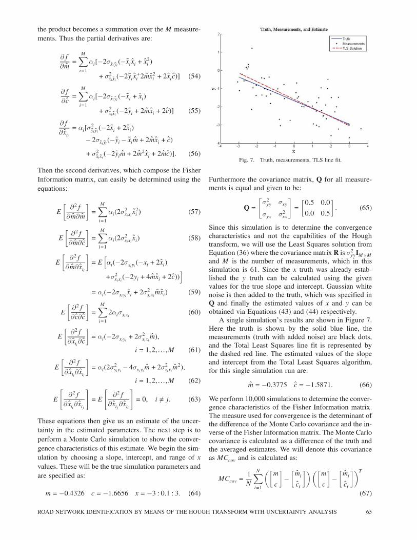
Fig. 12. Data set #2 line CRLB.

First we present the results for the estimated CRLBmatrix corresponding to the line estimate’s parameters.Figure 12 shows the three sigma bounded region forthe lines, which again due to the number of measure-ments associated with each of the lines, converges tosmall values for most lines. For a few straight line seg-ments which have very few associated measurements,the bounds are very lax.We supplement Figure 12 with an example of a

line’s CRLB estimate. Equation (77) refers to a linewhich has 1,034 measurements associated with it:264¾

2mm ¾mc ¾mx

¾cm ¾2cc ¾cx

¾xm ¾xc ¾2xx

375

=

264 2:2541e¡05 3:5129e¡ 09 ¡1:7855e¡ 093:5129e¡09 3:6176e¡ 10 ¡1:2573e¡ 10¡1:7855e¡ 09 ¡1:2573e¡10 1:4242e¡10

375(77)

which illustrates a high degree of confidence in theestimated model parameters. We must then use theJacobian transformation to obtain the covariance interms of x and y. A single measurement’s covariancematrix is given by the equation:"

¾2xx ¾xy

¾yx ¾2yy

#= 1:0e¡ 06£

·0:3850 ¡0:4209¡0:4209 0:8059

¸:

(78)

The Jacobian transformed CRLB is then added tothe measurement covariance defined in Equation (78)to produce the final covariance in the measurement in-

Fig. 13. Data set #2 error ellipses one sigma.

Fig. 14. Data set #2 mean line uncertainty.

cluding the covariance in the estimate given by Equa-tion (79):"

¾2xx ¾xy

¾yx ¾2yy

#= 1:0e¡06£

·0:3852 ¡0:4209¡0:4209 0:8089

¸:

(79)Figure 13 shows a few measurement’s one sigma el-lipses with the line estimate.Using the error ellipses we once again compute the

mean covariance in x and y. This covariance is thenused to represent a mean error in the line using onesigma we can see from Figure 14 that this encompassesthe majority of the data associated with each of the lineestimates.There are no ellipses identified in this data set but

there are a significant number of polynomial blends. Apolynomial blend in this data set typical contains from400 to 1,000 measurements. We present the results for apolynomial, which contains 1,032 associated measure-ments in Equation (80):

26664¾2AA ¾AB ¾AC ¾AD

¾BA ¾2BB ¾BC ¾BD

¾CA ¾CB ¾2CC ¾CD

¾DA ¾DB ¾DC ¾2DD

37775=266643:9162e¡ 12 2:9909e¡10 ¡2:0009e¡ 08 ¡1:5304e¡ 062:9909e¡ 10 2:2842e¡08 ¡1:5281e¡ 06 ¡0:0001¡2:0009e¡08 ¡1:5281e¡ 06 0:0001 0:0078

¡1:5304e¡06 ¡0:0001 0:0078 0:5980

37775 : (80)


5 CONCLUSION

This paper presents a systematic approach for theestimation of the road network from ground movingtarget data assuming the vehicles to be road based ve-hicles. The position locations of the multiple groundvehicles are used to generate a binary images, whichpermits using the Hough transform to identify straightline segments. Having identified the Hough parametersassociated with various straight line segments, the po-sition data associated with each of these straight linesegments is identified and used by a least squares algo-rithm to identify the parameters of a straight line, i.e.,slope and intercept. Since the two dimensional positiondata is contaminated with noise in both the dimensions,the total least squares is deemed the appropriate ap-proach for the estimation of the slope and intercept ofthe straight line segments. A detailed exposition of thetotal least squares approach for the estimation of themodel parameters is followed by the determination ofthe Cramer-Rao bounds on the estimated parameters. Amulti road network with numerous intersections is usedas a test case to illustrate the potential of the proposedapproach to estimate the road network and character-ize the associated uncertainty. Currently the proposedapproach is being extended to estimating curved sec-tion of roads which are assumed to be representable byarcs of ellipses. This will permit a parsimonious repre-sentation of the road-network by eliminating numerousstraight line segments which are necessary to representcurved sections of roads. A graphical user interface wasalso developed to permit a seamless estimation of road-network from ground vehicle kinematic data.

ACKNOWLEDGEMENT

This material is based upon work supported by theAFRL under Cooperative Agreement No. FA 8750-11-2-0082.

REFERENCES

[1] Tupin, Florence, Henri Maitre, Jean-Francois Mangin, Jean-Marie Nicolas, and Eugene PecherskyDetection of Linear Features in SAR Images: Applicationto Road Network Extraction.IEEE Transactions on Geoscience and Remote Sensing 36.2(1998).

[2] Koch, W., J. Koller, and M. UlmkeGround Target Tracking and Road Map Extraction.ISPRS Journal of Photogrammetry and Remote Sensing 61.3—4 (2006): 197—208.

[3] P. Gamba, F. Dell’Acqua, and G. LisiniImproving urban road extraction in high-resolution imagesexploiting directional filtering, perceptual grouping, andsimple topological concepts,IEEE Geosci. Remote Sens. Lett., vol. 3, no. 3, pp. 387—391,Jul. 2006.

[4] V. Amberg, M. Coulon, P. Marthon, and M. SpigaiStructure extraction from high resolution SAR data onurban areas,in Proc. IEEE Geosci. Remote Sens. Symp., 2004, vol. 3, pp.1784—1787.

[5] Hu, Jiuxiang, Anshuman Razdan, John C. Femiani, Ming Cui,and Peter WonkaRoad Network Extraction and Intersection Detection FromAerial Images by Tracking Road Footprints.IEEE Transactions on Geoscience and Remote Sensing 45.12(2007): 4144—4157.

[6] Aaron, Shackelford K., and Curt H. DavisUrban Road Network Extraction from High-ResolutionMultispectral Data.2nd GRSS/ISPRS Joint Workshop on Remote Sensing andData Fusion over Urban Areas, 2003, p. 142—146.

[7] Sklarz, S. E., Novoselsky A., and Dorfan M.Incremental Fusion of GMTI Tracks for Road Map Esti-mation.2008 11th International Conference on Information Fusion,Cologne, Germany, pp. 1—7.

[8] Halir, R. and Flusser, J.Numerically stable direct least squares fitting of ellipses.The Sixth International Conference in Central Europe. 1998.

[9] Duda, R. O. and P. E. HartUse of the Hough Transformation to Detect Lines andCurves in Pictures,Comm. ACM, Vol. 15, pp. 11—15 (January, 1972).

[10] Guil, N., and E. L. ZapataLower Order Circle and Ellipse Hough Transform.Pattern Recognition 30.10 (1997): 1729—1744.

[11] Tsuji, Saburo, and Fumio MatsumotoDetection of Ellipses by a Modified Hough Transformation.IEEE Transactions on Computers C-27.8 (1978): 777—781.

[12] Aguado, A. S., and M. S. Nixon“A New Hough Transform Mapping for Ellipse Detection.”Technical Report, University of Southampton, 1995.

[13] Crassidis, John L., and Yang ChengError-Covariance Analysis of the Total Least Square Prob-lem.Proceedings of the AIAA Guidance, Navigation and ControlConference, Portland, Oregon, August 8—11, 2011.

[14] Fitzgibbon, A. W. and Fischer, R. B.A buyer’s guide to conic fitting.Proc. of the British Machine Vision Conference. pp. 265—271.1995.

[15] Weisstein, Eric W.“Ellipse.”From MathWorld–A Wolfram Web Resource.http://mathworld.wolfram.com/Ellipse.html, Web. 18 Nov.2014.


Eric Salerno received his Masters of Science in Mechanical Engineering from theState University of New York at Buffalo (Buffalo, New York) in 2013 where hefocused his studies on estimation and control systems. He completed two internshipswith the Air Force Research Laboratory in Rome, New York where he worked ontest bedding Natural Language Processing algorithms and developing a Bayesianmodel for the estimation of remaining useable life for cellular devices in combatzones. He is currently pursuing a second Master's of Science in Computer Sciencefrom the State University of New York Polytechnic Institute (Utica, New York) aswell as his Certified Information Systems Security Professional certification andcurrently works at the Department of Defense.

Nagavenkat Adurthi is a graduate student at the University at Buffalo, pursuing aPh.D. degree. He has received his Bachelors from the Indian Institute of Technologyat Guwahati in 2010 and a Master's degree from the University at Buffalo in2013. He was recognized with the NAGS Distinguished Master's Thesis Awardfor the work on “The Conjugate Unscented Transform–An Approach to EvaluateMultidimensional Integrals.” His research interests include the fields of UncertaintyQuantification, Information Theory and State Estimation.

Tarunraj Singh is a fellow of ASME and AAAS. He received his B.E. degree fromBangalore University, Bangalore, India, a M.E. degree from the Indian Institute ofScience, Bangalore, and his Ph.D. degree from the University of Waterloo, Waterloo,ON, Canada, all in mechanical engineering. He was a Postdoctoral Fellow withthe Aerospace Engineering Department, Texas A&M University, College Station.Since 1993, he has been with the University at Buffalo, Buffalo, NY, wherehe is currently a Professor with the Department of Mechanical and AerospaceEngineering. He was a von Humboldt Fellow and spent his sabbatical at the IBMAlmaden Research Center in 2000{2001 and at RWTH Aachen in 2011. He was aNational Aeronautics and Space Administration Summer Faculty Fellow with theGoddard Space Flight Center in 2003. His research has been supported by theNational Science Foundation, Air Force Office of Scientific Research, NationalSecurity Agency, Office of Naval Research, and various industries, includingMOOG Inc. Praxair and Delphi Thermal Systems. He has published more than 200refereed journal and conference papers and has presented over 50 invited seminarsat various universities and research laboratories. His research interests are in robustvibration control, estimation, and intelligent transportation.


Puneet Singla (Ph.D., 2006, Texas A&M University) is an Associate Professorand director of graduate studies of Mechanical & Aerospace engineering at theUniversity at Buffalo. He has developed a vigorous research program in the generalarea of estimation and control with specific focus on uncertainty quantificationand characterization at University at Buffalo. He has authored over 100 papersto-date including one book and 27 journal articles covering a wide array ofproblems. He has received competitive NSF CAREER award for his work onUncertainty Propagation and Data Assimilation for Toxic Cloud Prediction andthe AFOSR Young Investigator Award for his work on Information Collection andFusion for Space Situational Awareness. He is a senior member of the AmericanInstitute of Aeronautics and Astronautics (AIAA), and member of the AmericanAstronautical Society (AAS), the American Society for Mechanical Engineers(ASME), the Institute of Electrical and Electronics Engineers (IEEE) and the Societyfor Industrial and Applied Mathematics (SIAM).

Adnan Bubalo received his M.S. degree in Computer and Information Science fromthe State University of New York Institute of Technology in 2009. He is presentlya Computer Scientist with the Air Force Research Laboratory (AFRL) InformationDirectorate in Rome, NY. Adnan is the Deputy Lead for the AFRL Processingand Exploitation (PEX) Core Technical Competency (CTC). His research interestsinclude target tracking, information fusion, and clustering.

Maria Cornacchia received her M.S. degree in Computer and Information Sciencefrom Syracuse University in 2009. Mrs. Cornacchia is also currently pursuing aPh.D. in Computer Information Science and Engineering from Syracuse University.She is a Computer Scientist with the Air Force Research Laboratory (AFRL)Information Directorate in Rome, NY. Her research interests include target tracking,information fusion, data mining, and computer vision.

Mark Alford received his M.S. degree in Electrical and Computer Engineering fromSyracuse University in 1988. He is presently an Electronics Engineer with the AirForce Research Laboratory (AFRL) Information Directorate in Rome, NY. Mark isthe primary in-house program manager for the Activity Based Analysis branch. Hehas a strong background in fusion and tracking and his research interests includeboth quantitative and qualitative intelligence analysis and reporting: primarily fromchat, video and images.


Eric Jones received his M.S. degree in Electrical Engineering from SyracuseUniversity in 1989. He is presently an Electronics Engineer with the Air ForceResearch Laboratory (AFRL) Information Directorate in Rome, NY. His researchinterests include multiple target tracking, nonlinear filtering, and image analysis.


Documents

Automatic cartographic feature extraction has been Road ...code.eng.buffalo.edu/jrnl/Road_Estimation.pdf · Road Network Identification by means of the Hough Transform with Uncertainty