Automatic Calibration of Storm Water Management Model (SWMM) with Multi-objective Optimization

by

Mina Shahed Behrouz

August 1, 2018

A thesis submitted to the

Faculty of the Graduate School of

the University at Buffalo, State University ofNew York

in partial fulfillment of the requirements for

the degree of

Master of Science

Department of Civil, Structural, and Environmental Engineering

Acknowledgements

I would like to take this opportunity to express my sincere appreciation to my MS advisor Dr. Zhu

for guiding me throughout my graduate school career. His guidance and patience over the last two

years have helped me to grow academically, professionally, and personally.

Next I would like to thank Dr. Rabideau and Dr. Matott for serving as my committee members. I

am extremely grateful for their assistance and suggestions throughout my MS thesis .

I would also like to thank my parents for their motivation and unconditional support that they have

always provided me with. Without their support, this journey would not have been possible.

In addition, I thank the Department of Civil, Structural, and Environmental Engineering at the

University at Buffalo for providing me with a tuition scholarship as well as a full time assistantship

for my master' s studies.

ii

Table of Contents

Abstract ........................................................................................................................................ viii

1. Introduction and background ................................................................................................... 1

2. Literature review ...................................................................................................................... 4

2.1. SWMM Process Models ................................................................................................... 4

2.1.1. External forcing data ................................................................................................. 4

2.1.2. Land-surface runoff component.. .............................................................................. 5

2.1.3. Subsurface groundwater component.. ....................................................................... 6

2.1.4. Conveyance system component ................................................................................ 7

2.2. Sensitivity analysis ........................................................................................................... 9

2.3. Calibration ...................................................................................................................... 16

3. Methodology.......................................................................................................................... 18

3.1. OSTRICH-SWMM ........................................................................................................ 18

4..................................................................................................................................................... 20

4.1. Objectives and Algorithms ............................................................................................. 20

4.1.1. ObjectiveFunction used in OSTRICH ............................................................................ 20

4.1.2. Algorithms implemented in OSTRICH ......................................................................... 21

4.1.3. Objective Functions ........................................................................................................ 22

5. Study Area ............................................................................................................................. 24

5.1. Catchment Description ................................................................................................... 24

5.2. Flow and rainfall monitoring data .................................................................................. 26 iii

5.2.1. Rainfall data ............................................................................................................ 26

5.2.2. Flow data ................................................................................................................. 26

5.3. Base SWMM model ....................................................................................................... 27

5.4. Sensitivity analysis and variables ................................................................................... 29

6. Results ................................................................................................................................... 31

6.1. Sensitivity Analysis ........................................................................................................ 31

6.2. Range of calibrated parameters ...................................................................................... 31

6.3. Single objective calibration ............................................................................................ 33

6.4. Multi-objective calibration including peak flow and average flow ............................... 35

6.5. Multi-objective calibration with consideration of time series of flow data ................... 38

6.6. Goodness of fit measures ............................................................................................... 43

7. Discussion.............................................................................................................................. 46

8. Summary and Conclusion ...................................................................................................... 48

9. References ............................................................................................................................. 49

iv

List of Figures

Figure 1 - SWMM processes and input parameters ....................................................................... 8

Figure 5 - Observed and simulated flow data from manually calibrated base SWMM model for

Figure 6 - Sensitivity analysis of study domain with respect to a) peak flow and b) average flow

Figure 7- set of Pareto optimal solutions for a two-objective calibration including, peak flow and

Figure 8 - set of Pareto optimal solutions for a two-objective calibration including, peak flow and

Figure 9 - set of Pareto optimal solutions for a two-objective calibration including, average flow

and RMSE. The single objective solution with respect to average flow and peak flow were

Figure 10 - predicted versus observed flow for a) base model, calibration considering b) Obj_l ,

Figure 2 - OSTRICH-SWMM linkage ......................................................................................... 20

Figure 3 - Sub-model location map .............................................................................................. 25

Figure 4 - Mean and standard deviation of seven rain gauges located in the study domain ........ 27

calibration and validation time periods ......................................................................................... 28

....................................................................................................................................................... 32

average flow. The single objective solutions were also shown by pink and orange points .......... 38

RMSE. The single objective solution with respect to peak flow and average flow were shown by

pink and orange points, respectively ............................................................................................. 39

shown by orange and pink points, respectively ............................................................................ 39

c) Obj_2, d) Obj_l and Obj_2, e) Obj_l and Obj_3 , f) Obj_2 and Obj_3 , g) Obj_l , Obj_2, and

Obj_3. Line of equality is shown by dot in each one.................................................................... 45

Figure 11 - An example to highlight the importance of time delay analysis .............................. 47

V

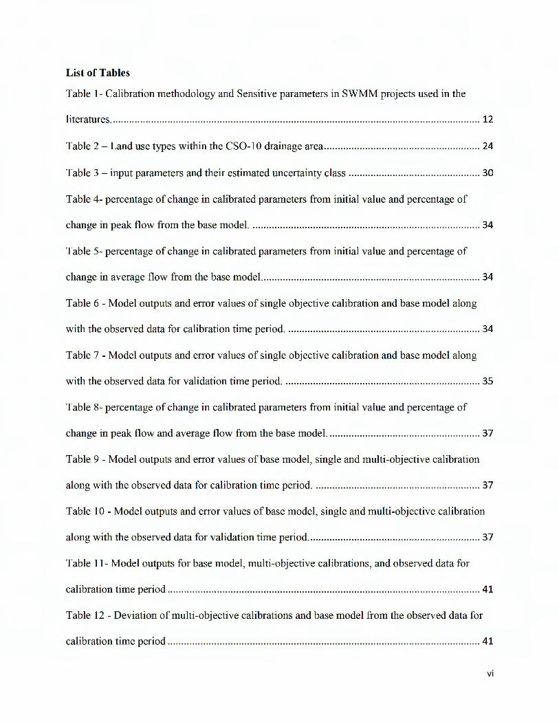
List of Tables

Table 1- Calibration methodology and Sensitive parameters in SWMM projects used in the

literatures....................................................................................................................................... 12

Table 4- percentage of change in calibrated parameters from initial value and percentage of

Table 5- percentage of change in calibrated parameters from initial value and percentage of

Table 6 - Model outputs and error values of single objective calibration and base model along

Table 7 - Model outputs and error values of single objective calibration and base model along

Table 8- percentage of change in calibrated parameters from initial value and percentage of

Table 9 - Model outputs and error values of base model, single and multi-objective calibration

Table 10 - Model outputs and error values of base model, single and multi-objective calibration

Table 11- Model outputs for base model, multi-objective calibrations, and observed data for

Table 12 - Deviation of multi-objective calibrations and base model from the observed data for

Table 2 - Land use types within the CSO-10 drainage area ......................................................... 24

Table 3 - input parameters and their estimated uncertainty class ................................................ 30

change in peak flow from the base model. ................................................................................... 34

change in average flow from the base model.. .............................................................................. 34

with the observed data for calibration time period . ...................................................................... 34

with the observed data for validation time period ........................................................................ 35

change in peak flow and average flow from the base model. ....................................................... 37

along with the observed data for calibration time period . ............................................................ 37

along with the observed data for validation time period ............................................................... 37

calibration time period .................................................................................................................. 41

calibration time period .................................................................................................................. 41

vi

Table 13 - Model outputs for base model, multi-objective calibrations, and observed data for

validation time period ................................................................................................................... 41

Table 14 - Deviation of multi-objective calibrations and base model from the observed data for

validation time period ................................................................................................................... 42

vii

Abstract

Among various hydrologic models that are available to simulate urban runoff, the Storm Water

Management Model (SWMM) is the most widely used numerical model. A typical SWMM project

has about hundreds or thousands of sub-catchments and for each sub-catchment, there are more

than 20 parameters associated with six different physical processes. Estimating all of these

parameters are practically impossible, so model calibration is a challenging task. Manual

calibration is used mostly but requires significant efforts and stops once simulation results are

"satisfactory". Some studies have adopted automatic calibration using a single objective

optimization. However, an optimal parameter set obtained for one objective (e.g. peak flow) may

perform poorly for another objective (e.g. average or low flow). In this study, SWMM was

integrated with OSTRICH (Optimization Software Tool for Research Involving Computational

Heuristics) to perform automatic multi-objective calibration. A sub-catchment within Buffalo, NY

was selected as a case study. Automatic calibration using single and multiple objectives were

conducted and compared. OSTRICH-SWMM is proved to be a useful tool for calibrating SWMM

models. This study shows multi-objective calibration provides a more robust parameter set than

any single objectives. A Pareto front is obtained in multi-objective calibration so an optimal

solution can be selected according to trade-off Moreover, this study highlights the importance of

determining and considering time delay between simulated and observed values in model

calibration.

viii

1. Introduction and background

Urbanization is associated with continuous mcreases m impervious area. Increasing

impervious area leads to the increase of total runoff volume and peak flow that detrimentally

impact the drainage and waterway systems. Nowadays, various hydrologic models are available

to simulate the urban runoff, including HEC-1 (U.S. Army Corps of Engineers 1985), TR-20 and

TR-55 (Soil Conservation Service 1983, 1986), MOUSE (Danish Hydraulic Institute 1995),

HydroWorks (HR Wallingford Ltd. 1997), and Storm Water Management Model (SWMM)

(Huber and Dickinson 1988). Among the available models, SWMM, a public domain software

developed by United States Environmental Protection Agency (U.S. EPA), is the most widely used

and popular numerical model for managing the urban runoff quantity and quality in the world

(Obropta and Kardos 2007). SWMM can be implemented for both single-event and long-term

precipitation time series on catchments that have storm drains, combined sewer systems, sanitary

sewer systems, and other drainage systems in urban areas.

SWMM requires a large number of variables and parameters to sufficiently express the

complex relationship between rainfall, runoff, and watershed characteristics. Estimation of all of

the parameters is a hard task since detailed information about structure and geometrical properties

of a drainage network is often unavailable or incomplete (Cooper et al. 2007) Hence, model

calibration needs to be adopted in order to optimize the parameters ofthe SWMM model by getting

a good fit between the field-measured observations and model-computed predictions. Prior to

performing calibration, sensitivity analysis needs to be implemented to narrow the number of

parameters from the large number ofparameters in the model. The results ofthe sensitivity analysis

identify the relative impact of each model input parameter on the model outputs and adequately

find and rank the most sensitive parameters (Niazi et al. 2017). Sensitivity analysis is typically

1

carried out manually by changing the value of each input parameter while keeping all other

parameters constant (van der Sterren et al. 2014; James et al. 2002). There are more complex

methods available to perform sensitivity analysis such as artificial neural network (Zaghloul and

Abu Kiefa 2001 ), Generalized Likelihood Uncertainty Estimation (Sun et al. 2014b), and Multi­

objective Generalized Sensitivity Analysis (Knighton et al. 2016).

The key parameters identified during the sensitivity analysis are then used to calibrate the

model. The calibration process can be either done manually or automatically. Manual calibration

is a process made by a manual trial and error approach which is a common practice in industry and

performed by changing the value of one parameter at a time and comparing the SWMM simulated

with observed runoff in the outlets. However, there is no guarantee that the optimal parameter

values will be found since the calibration is stopped when the results are satisfactory based on the

defined criteria. Model verification criteria for total flow volume, peak flow, and time to peak have

been provided in Shamsi and Koran (2017).

Automatic calibration exists to overcome the shortcomings of manual calibration by taking

advantage of optimization algorithms as well as improving the accuracy and reliability of the

models. Automatic calibration has the ability to optimize a user-defined objective function in

which the linked software to SWMM perturbs model parameters and runs the SWMM model until

the defined objective function is satisfied. Different automatic calibration algorithms are based on

gradient-based methods (e.g. , steepest descent, conjugate gradient), combinatorial methods (e.g. ,

the simplex method), and heuristic methods (e.g. , genetic algorithms (GA), shuffled complex

evolution algorithms). Gradient-based methods require a smaller number ofmodel runs to find the

optimal values of the parameters; however, they may get trapped in local minimal if the initial

estimate of the parameter is not chosen properly (Abrishamchi et al. 2010; Mancipe-Munoz et al.

2

2014). Combinatorial methods aims to find the optimal value of parameters from a finite set of

values and therefore there is no guarantee to find an optimal solution. Heuristic methods are better

capable of finding the global minimal, although it require a larger number of model runs (Duan et

al. 1994; Liong et al. 1993).

According to literature review of 22 studies that performed automatic calibration (refer to

Table 1 ), 17 studies adopted single objective calibration. Although the obtained parameters set

performs well for the objective function considered in the optimization, it may not perform well

for other objective functions . Multi-objective calibration can work better by considering two or

more objectives. Furthermore, often the developed research code is not available to public domain,

is time-consuming to be used for complex drainage systems, cannot be run in parallel, and only

includes one type of optimization algorithm.

An open source calibration and optimization tool named OSTRICH (Optimization Software

Tool for Research Involving Computational Heuristics) was linked to SWMM which provides

possibility of dozens of algorithms, many of which are parallelized. It is a useful tool to be applied

to real and complex drainage systems. By implementing OSTRICH-SWMM for a case study in

Buffalo, New York, automatic single and multi-objective calibrations were performed and

assessed. Single objective calibrations can be performed using objective functions based on peak

flow, average flow which is equivalent to total flow volume, or time series of flow data separately.

Multi-objective calibration includes two or more of the aforementioned aspects of flow. The

simulation period was split into a four-month calibration period (9/15/2016 to 1/15/2017) and a

three-month validation period (3/15/2017 to 6/15/2017). Each calibration effort was done on the

calibration time period and the resulted calibrated parameters were used for the validation time

period.

3

2. Literature review

2.1. SWMM Process Models

SWMM simulates runoff quantity and quality from urban and suburban areas. There are six

primary environmental components within SWMM that are (Huber et al. 1988; Rossman 2015):

2.1.1 External forcing data including precipitation, temperature, evaporation, and wind speed

2.1.2 Land surface runoff component

2.1.3 A subsurface groundwater component

2.1.4 A conveyance system of pipes, channels, flow regulators, and storage units

2.1.5 Contaminant buildup, wash-off, and treatment

2.1.6 LID controls

Not all of the mentioned processes need to be included in a project. In most of the projects,

only precipitation, land-surface runoff, groundwater component, and conveyance system are

included. Four of the SWMM processes that are used the most in SWMM projects are elaborated

on hereunder.

2.1.1. External forcing data

SWMM is capable of simulating either single-event or long-term precipitation time series. Air

temperature data are imported when modeling snowfall and snowmelt processes. A certain

temperature threshold, specified by user, is needed to consider precipitation in the form of snow.

Evaporation data can be provided into the SWMM as a single constant value, average monthly

values, or time-series daily data. Wind speeds are used for simulating snowmelt and can be

imported as average monthly values or as daily time series.

4

2.1.2. Land-surface runoff component

2.1.2.1. Surface runoff:

SWMM divides the area to be modeled into one or several subcatchments. Each subcatchment

is treated as a nonlinear reservoir with a uniform slope (Shubinski et al. 1973). By considering

each subcatchment as a nonlinear reservoir, a water balance equation is employed over each

subcatchment. The change in depth of water over the subcatchment as a function of time is the

difference between the inflows; sum of precipitation and flow from upstream subcatchments; and

outflows; sum of evaporation, infiltration, and surface runoff

Each subcatchment in SWMM can be divided into two subareas; pervious area and two

impervious subareas. Surface runoff can infiltrate into the upper soil layer of the pervious subarea,

but not into the impervious subarea. Impervious areas are also divided into two subareas; one with

and one without depression storage. Runoff flow from each of the subareas can be routed

independently to the other subareas or drained to the subcatchment outlet.

2.1.2.2. Infiltration:

Infiltration is the process of rainfall penetrating the ground surface into the unsaturated soil

zone of pervious subcatchment. There are several ways to estimate the volume and/or the rate of

infiltration into a soil, including Horton's method (Horton 1940), modified Horton method, Green­

Ampt method (Green and Ampt 1911 ), modified Green-Ampt method, and Curve number method

(Akan and Houghtalen 2003).

Horton's method is based on an empirical approach that assumes infiltration decreases

exponentially from an initial maximum infiltration rate and decreases to a minimum infiltration

rate over time. Input parameters required by this method include the maximum and minimum

infiltration rates (MaxRate and MinRate) and a decay coefficient (Decay) which determines how

5

fast the rate decreases over time. As this method is valid only when the rainfall intensity at all

times exceeds the infiltration rate, modified Horton method was introduced that presents a more

accurate prediction of infiltration when rainfall intensity is low.

Green and Ampt method predicts cumulative infiltration as a function of time and soil

properties. This method assumes that a wetting front exists in the soil column and separates the

soil into two layers. The soil above the wetting front is assumed to be uniformly saturated and the

soil below the wetting front has some initial moisture content. Wetting front advances at the same

rate as water infiltrates into the soil and the volumetric water contents below the advancing wetting

front is assumed to be constant. The input parameters are initial moisture deficit (InitDef), the

soil's hydraulic conductivity (Conduct), and the suction head at the wetting front (Suction).

Curve number method is based on an empirical equation that relates cumulative infiltration to

cumulative precipitation by taking advantage of Soil Conservation Service (SCS) curve number

that has been tabulate and is available for different soil groups and land uses.

2.1.3. Subsurface groundwater component

The groundwater component receives water penetrating into the soil as a result of infiltration

from the land surface component that affects the groundwater table. Subsurface flow is simulated

by dividing the soil beneath each subcatchment into two zones: the upper and lower zone. The

upper zone is unsaturated and its moisture content assumed to be uniformly distributed. The lower

zone is assumed to be fully saturated. Water penetrating into the soil, flows from the upper zone

to the lower zone. The water in the lower zone can be either directed into the conveyance system

of pipes or percolate downward. To model the groundwater component, a water balance 1s

performed on the two layers to simulate the dynamics of storage and flow from each layer.

6

2.1.4. Conveyance system component

There are two ways to model flow routing in SWMM: kinematic wave routing and dynamic

wave routing. The two methods implement the Manning equation to relate flow rate to flow depth

and bed slope. The kinematic wave routing method implements the continuity equation with the

simplified assumption that the water surface slope is equal to the bottom slope of the conduit in

each conduit. This method is unable to present backwater effects, entrance/exit losses, or

pressurized flow. However, the dynamic wave model overcomes the mentioned limitations by

solving the complete one-dimensional Saint Venant equations that implements continuity and

momentum equations for conduits and mass equations for nodes.

7

I I

Precipitation Surface Runoff

\..

DS_imperv, DS_perv, N_imperv, N_perv,

%Imperv, %Slope, Area, Width, %Zero_imperv

____________ ,.

-----------...~------1

Overland flow

Height, Thick, V_ratio, K_sat --------------•

, Ir

LID Controls .~ ~

/

\.

, r

Evaporation/ Infiltration

'I

~

\.

14------------

, Ir 1 r

Buildup Washoff Groundwater ,

InitSat, MaxRate, MinRate,

Decay, Suction,

Conduct, InitDef, CurveNo

...,,

FC, UMC,

Ps, Ks,

CET, DP

/

[ Rough, Length, Width_C ]----------• ------------------ l I I I I I 1 .. I

I ,,,--------"----- I I I

Sanitary Flows l ~

~ Channel, Pipe & Storage Routing

, "'

,l

\.

Treatment/ Rainfall- Dependent Inflow Diversion and Infiltration

\.

Figure J - SWMMprocesses and input parameters

8

2.2. Sensitivity analysis

SWMM has four principle hydrologic/hydraulic processes that have been described in section

2.1. The hydrologic processes are precipitation, evaporation, surface runoff, infiltration,

groundwater flow, snow packs and snow melts. The hydraulic processes are the drainage system

network of pipes, channel, storage/treatment units and diversion structures.

It is necessary to perform a detailed sensitivity analysis of a SWMM project to identify the

main parameters of the SWMM which would be the most effective in the simulation of a rainfall­

runoff-routing model (Rossman 2009). Sensitivity analysis has been characterized as an integrated

part in building and evaluating the performance of models (Jakeman et al. 2006). Identified

sensitive parameters in a project are considered during the calibration process.

Generally speaking, there are two main groups of sensitivity analysis: local and global

approaches (Saltelli et al. 1999). Local sensitivity analysis evaluates how the outputs change by

varying one input parameter at a time. On the contrary, the global sensitivity analysis (GSA)

considers a variation of all parameters simultaneously and evaluates their contribution to the

uncertainty of outputs. Common used GSA methods include variance-based methods (Sobol

1990), sampling-based methods such as Latin hypercube sampling with partial rank correlation

coefficient index (LHS-PRCC) (Helton and Davis 2002), global screening methods (Morris 1991),

regression-based methods and others (Freni and Mannina 2012).

SWMM often reports the output results in the form of various time senes, including

(hydrographs or pullutographs). Aggregate values can then be extracted from the time series,

including peak discharge, peak discharge time, total volume, and total depth. One approach to do

sensitivity analysis is to compare calculated aggregate quantities before and after performing

perturbing the targeted parameter (Niazi et al. 2017).

9

Niazi et al. (2017) reviewed previous studies and reported the sensitive parameters by

considering the runoff quantity as the output variable. Table 1 shows the sensitive parameters

reported in each paper along with the method subsequently used for calibration. Figure 1 shows

the processes that SWMM was built upon, their interactions, and the sensitive parameters for each

process. Despite the fact that the sensitiveness of input parameters are greatly project-specific, the

most common sensitive parameters, reported at least 10 times in 50 papers, are: Rough, ¾Imperv,

DS_imperv, N_imperv, N_perv, DS_perv, Width, and infiltration parameters. These parameters

are bolded in Figure 1.

The abbreviation of sensitive parameters are as follows (the numbers in parenthesizes state how

many times each parameter appears out of 42 papers):

► Impervious surfaces characteristics, including:

o Dstore-Imperv, depth of depression storage on the impervious portion of the subcatchment

(18)

o N-Imperv, Manning' s n for overland flow over the impervious portion of the

subcatchment (26)

o % Imperv, percent ofland area that is impervious (19)

o ¾Zero-Imperv, percent of the impervious area with no depression storage (2)

► Pervious surfaces characteristics, including:

o N-Perv, Manning ' s n for overland flow over the pervious portion of the subcatchment (19)

o Dstore-perv, depth ofdepression storage on the pervious portion of the subcatchment (15)

► Soil infiltration parameters, including:

o InitSat, percent to which the LID unit's soil layer or storage layer is initially filled with

water (2)

10

o MaxRate, maximum infiltration rate on Horton infiltration (9)

o MinRate, minimum infiltration rate on Horton infiltration (10)

o Decay, decay rate constant of Horton infiltration (7)

o Suction, soil capillary suction in Green-Ampt infiltration ( 4)

o Conduct, soil saturated hydraulic conductivity in Green-Ampt infiltration (8)

o InitDef, initial soil moisture deficit in Green-Ampt infiltration (6)

o CurveNo, SCS curve number (1)

► Subcatchment characteristics, including:

o Width, characteristic width of the overland flow path for the sheet flow runoff (19)

o %Slope, average percent slope of the subcatchment (10)

o Area, area of subcatchment ( 4)

► LID parameters, including:

o Height, thickness of storage layer ( 1)

o Thick, thickness of soil layer/permeable pavement (1)

o Vratio, void ratio (1)

o Ksat, soil ' s saturated hydraulic conductivity, initial concentration (1)

► Conduit parameters, including:

o Rough, Manning's n for conduit/open channel (15)

o Length, length of conduit/open channel (3)

o Width-C, width of conduit/open channel (2)

► Groundwater parameters, including:

o FC, soil field capacity (2)

o UMC, unsaturated zone moisture content at start of simulation (2)

o Ps, slope of soil tension versus moisture content curve (1)

11

o Ks, slope of the logarithm of hydraulic conductivity versus moisture deficit (2)

o CET, maximum evapotranspiration rate assigned to the upper zone (1)

o DP, coefficient for unquantified losses (1)

o Al , groundwater flow coefficient (1)

o B 1, groundwater flow exponent ( 1)

o PR, porosity (1)

o WP, wilting point ( 1)

o DET, transpiration depth (1)

Table 1- Calibration methodology and Sensitive parameters in SWMMprojects used in the literatures.

Reference

Alamdari (2016)

Baek et al. (2015)

Balascio et al. (1998)

Barco et al. (2008)

Beling et al. (2011)

Blumensaat(2012)

Borris et al. (2014)

Burszta-Adamiak and

Mrowiec (2013)

Carvalho et al. (2011)

Method*

NSGAII

LH-OAT

GA

Complex

method

Manually

Manually

Manually

Manually

NSGAII

Sensitive parameters

Width, ¾Imperv

N-Perv, N-Imperv, Rough

¾Imperv, Dstore-Imperv, % Zero-Imperv,

Width, % Slope, N-Imperv, N-Perv, Dstore­

perv, MaxRate, MinRate, Decay

Dstore-Imperv, Dstore-Perv

¾Imperv, N-Imperv, N-Perv, Dstore-Perv,

Dstore-Imperv, MaxRate, MinRate, Decay

Width

Dstore-Imperv, Dstore-Perv

InitSat

N-Imperv, N-Perv, ¾Imperv, MaxRate,

MinRate

12

Table 1. (Continued)

Cermola et al. (1979)

Chen and Adams (2006)

Chow et al. (2012)

Chung et al. (2011)

Dent et al. (2004)

Fang and Ball (2007)

Fioretti et al. (2010)

Giilbaz and Kazezy1lmaz-

Alhan (2013)

Herrera et al. (2006)

Hsu et al. (2000)

James et al. (2002)

James and Kuch (1998)

Krebs et al. (2013)

Krebs et al. (2014)

Lei and Schilling (1994)

Manually

Manually

Manually

Manually

GA

GA

Manually

Manually

NSGAII

Manually

GA

PEST

NSGAII

NSGAII

Manually

¾Imperv, Width

Area; % Slope, Dstore-Imperv, Dstore-Perv,

N-Imperv, N-Perv, MinRate, MaxRate

¾Imperv, Width, Dstore-Imperv, N-Imperv

N-Perv, N-Imperv, Dstore- Imperv, Dstore-

Perv, Rough, Conduct, FC, UMC, Ks, Ps,

CET, DP

Area

¾Imperv, Width, N-Imperv, Dstore-Imperv

Dstore-Imperv, N-Imperv

Rough,N-Imperv,N-Perv, N-Conduct,

Conduct, InitSat, InitDef, Dstore-Imperv,

Dstore-Perv

Suction, Conduct, InitDef, N-Perv, Dstore-

Perv, Width, FC, UMC, Ks, Al , Bl , PR,

WP, DET

N-Imperv

Area, %Imp, Width, N-Imperv, N-Perv, %

Slope

% Zero-Imperv, Dstore-Imperv, Width, %

Slope, Dstore-Perv, N-Perv, MaxRate,

MinRate, Decay

Dstore-Imperv, Rough

¾Imperv, Dstore-Imperv, Dstore-Perv, N-

Imperv, N-Perv, Rough, Suction, Conduct,

InitDef

¾Imperv

13

Table 1. (Continued)

Li et al. (2014)

Liong et al. ( 199 5)

Mancipe-Munoz et al. (2014)

Peterson and Wicks (2006)

Qin et al. (2013)

Rosa et al. (2015)

Shinma and Reis (2011)

Shinma and Reis (2014)

Sun et al. (2014a)

Sun et al. (2014b)

Tan et al. (2008)

Temprano et al. (2006)

Tsihrintzis and Hamid (1998)

Tsihrintzis et al. (2007)

Warwick et al. (1991)

LH

GA

PEST

Manually

Manually

OAT± 50%

NSGAII

NSGAII

GLUE

GLUE

PEST

Manually

Manually

Manually

Manually

Rough, Area, Width, N-Imperv, N-Perv,

MinRate, % Slope

N-Perv, Dstore-Perv, MaxRate, MinRate,

Decay, Width, ¾Imperv, % Slope

¾Imperv, Width, % Slope, N-Imperv,

Dstore-Imperv, N-Perv, Dstore-Perv; If

imperviousness <20%:

Suction, Conduct, InitDef

Rough, Length, Width-C

Height, Vratio, Thick, Ksat

With LID: Conduct, N-swales, InitDef

Without LID: Conduct, InitDef, N-Imperv

¾Imperv, N-Perv, Rough, MaxRate,

MinRate, Decay

N-Imperv, N-Perv, MaxRate, MinRate,

Decay, Rough

N-Imperv, N-Perv, Dstore-Imperv, Dstore-

Perv; Width, Rough

Dstore-Imperv, N-Imperv, Rough, width,

Dstore-Imperv, Dstore-tree, N-tree

Width, ¾Imperv, % Slope, N-Imperv

¾Imperv, % Slope, Width, N-Imperv, N-

Perv

Dstore-Imperv, Rough, N-Imperv, N-Perv,

Dstore-Perv, Suction, Conduct, InitDef

Rough

¾Imperv

14

Table 1. (Continued)

Wu et al. (2008) Manually % Slope, Dstore-Imperv, Dstore-Perv, rough,

Length, Width-C, CurveNo

Zaghloul (1983) Manually ¾Imperv, Width, Dstore-Imperv, Dstore­

Perv, N-Imperv, N-Perv, % Slope, Length,

Rough, MaxRate, MinRate, Decay

Zaghloul and Al-Shurbaji Manually Dstore-Imperv, Width, N-Imperv

(1990)

Zahmatkesh et al. (2015) DREAM CurveNo

Zhao et al. (2008) GLUE Des-Imperv; ¾Imperv, N-Imperv, Width

*OAT: One-factor-At-a-Time; GA: Genetic Algorithm; LH: Latin Hypercube; NSGA: Non­

dominating Sorted Genetic Algorithm; PEST: Parameter Estimation Tool; GLUE: Generalized

Likelihood Uncertainty Estimation; DREAM: DiffeRential Evolution Adaptive Metropolis, an

adaption of the shuffled complex evolution Metropolis

15

2.3. Calibration

Calibration is typically performed by adjusting model parameters within reasonable ranges

until a reasonable agreement is achieved between the observed data and model-simulated values.

The parameters such as geometric watershed characteristics, length of the channels, bottom slope

of the channels, and width of the channels that can be defined with good accuracy were considered

as a fixed value and therefore were excluded from the calibration process. The only parameters

being adjusted in the calibration are the sensitive model parameters that either cannot be easily

measured or cannot be measured with certainty.

Two approaches have been used for calibration of SWMM models: manual calibration and

automatic calibration. Manual calibration is performed by changing the value of each parameter

within a range that has been identified based on experience, previous studies, or combination of

both and comparing the field-measured data with simulated results. The process is continued until

a satisfactory match is achieved between the field-measured data and simulated results. This

method is labor intensive and time-consuming, especially when the catchment is large and

complex. Furthermore, it requires extensive familiarity with model operation and structure.

Moreover, there is no guarantee that the optimal solution will result. Automatic parameter

estimation and calibration methods have been implemented to overcome these difficulties and is

becoming increasingly used for calibration of rainfall-runoff models . Automatic calibration is

performed by a computer algorithm that perturbs the model parameters and examines the SWMM

model outputs with observed data until the user defined objective function is satisfied.

Some of the optimization algorithms/methods that were coupled with SWMM and used in

automatic calibration have been provided in Table 1. Optimization algorithms are based on

gradient-based method, combinatorial methods, heuristics approaches, or evolutionary algorithms.

16

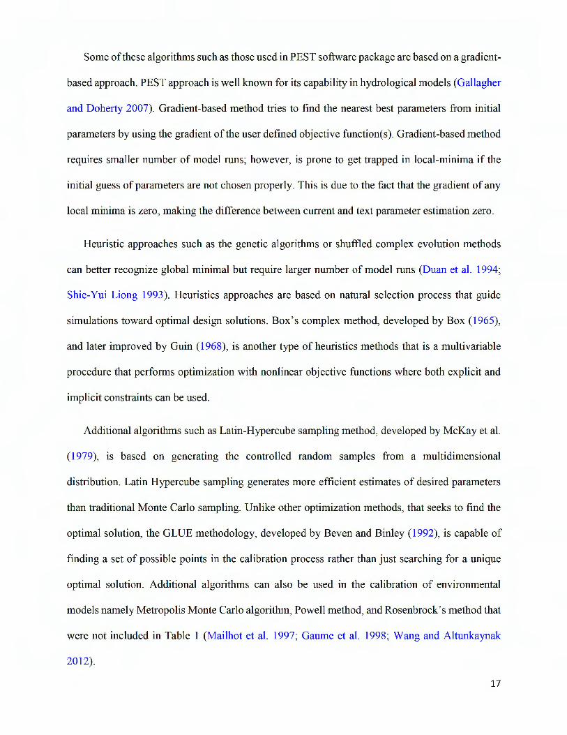
Some ofthese algorithms such as those used in PEST software package are based on a gradient­

based approach. PEST approach is well known for its capability in hydrological models (Gallagher

and Doherty 2007). Gradient-based method tries to find the nearest best parameters from initial

parameters by using the gradient of the user defined objective function( s ). Gradient-based method

requires smaller number of model runs; however, is prone to get trapped in local-minima if the

initial guess of parameters are not chosen properly. This is due to the fact that the gradient of any

local minima is zero, making the difference between current and text parameter estimation zero.

Heuristic approaches such as the genetic algorithms or shuffled complex evolution methods

can better recognize global minimal but require larger number of model runs (Duan et al. 1994;

Shie-Yui Liong 1993). Heuristics approaches are based on natural selection process that guide

simulations toward optimal design solutions. Box's complex method, developed by Box (1965),

and later improved by Guin (1968), is another type of heuristics methods that is a multivariable

procedure that performs optimization with nonlinear objective functions where both explicit and

implicit constraints can be used.

Additional algorithms such as Latin-Hypercube sampling method, developed by McKay et al.

(1979), is based on generating the controlled random samples from a multidimensional

distribution. Latin Hypercube sampling generates more efficient estimates of desired parameters

than traditional Monte Carlo sampling. Unlike other optimization methods, that seeks to find the

optimal solution, the GLUE methodology, developed by Beven and Binley (1992), is capable of

finding a set of possible points in the calibration process rather than just searching for a unique

optimal solution. Additional algorithms can also be used in the calibration of environmental

models namely Metropolis Monte Carlo algorithm, Powell method, and Rosenbrock's method that

were not included in Table 1 (Mailhot et al. 1997; Gaume et al. 1998; Wang and Altunkaynak

2012).

17

3. Methodology

3.1. OSTRICH-SWMM

OSTRICH is an open source model independent optimization and calibration tool that can be used

for calibration of model parameters and downloaded from

(www.eng.buffalo.edu/-lsmatott/software.html). OSTRICH contains a wide variety of

optimization algorithms applicable for automated calibration. The diverse set of algorithms

includes, but not limited to Genetic Algorithms (Goldberg 1989), Dynamically Dimensioned

Search (Tolson and Shoemaker 2007), Particle Swarm Optimization (Kennedy et al. 2001 ), and

Powell ' s Algorithm (Powell 1977). Most of these algorithms are parallelized, which allows the

user to take advantage of computing resources available at the Center for Computational Research

(CCR) at the University at Buffalo (UB). Previously, OSTRICH has been successfully

implemented in calibration and optimization of water resources engineering, groundwater

remediation (Bartelt-Hunt et al. 2006; Matott et al. 2009; Matott et al. 2006a; Matott et al. 2011 ;

Matott et al. 2006b; Matott et al. 2012), and environmental modeling systems such as FRAMES

(Johnston et al. 2011 ) and MESH (Haghnegahdar et al. 2014). In this research, OSTRICH was

linked with SWMM, the most widely used software in application of urban water management, to

perform automated calibration of SWMM models.

OSTRICH requires the modeling program with which it is linked to utilize text-based input

and output file format. As SWMM outputs are in binary file format, a python script named

SWMMtoolbox (https://pypi.python.org/pypi/swmmtoolbox) was used to conduct post-processing

and convert the binary output files to text-based format that is readable to OSTRICH.

OSTRICH is driven by a configuration file and a set of model template files. In OSTRICH

configuration file , user can select the type of optimization algorithm to be used, specify the model

executable file , select objective function, include template files and required model input files,

18

define the calibration parameters along with their initial values, upper, and lower bounds for each

of them, include observation variables, and identify response variables to be extracted from

SWMM binary output files through SWMMtoolbox. SWMM binary output files contain flow,

depth, and velocity at each node and link.

The structure of the template files should be identical to the corresponding model input file

except that the value of each calibration parameters is replaced with a unique mnemonic defined

in the configuration file. By implementing OSTRICH-SWMM for calibration, OSTRICH uses the

template files to generate different model input files with perturbed model parameters. For each of

the input files , OSTRICH runs the defined executable model program, uses observation variables

to read and extract the simulated observations from model output files , and compute the objective

function. This process continues until the objective function converges to a value identified by

user or completes a user-defined number of iterations. Figure 2 illustrates this process. For more

information of OSTRI CH and its features refer to OSTRI CH user manual (Matott 2017).

19

OSTRICH Model Templates

Confi2.

Result Model Input Model Output

SWMM5.exe

Figure 2 - OSTRICH-SWMM linkage

4.

4.1. Objectives and Algorithms

4.1.1. ObjectiveFunction used in OSTRICH

There are two types of ObjectiveFunction available within OSTRICH; WSSE (Weighted Sum

of Squared Error) and GCOP (General-purpose Constrained Optimization Platform).

When ObjectiveFunction is set to WSSE, OSTRICH will report only one set of model

parameters in which the value ofthe WSSE is the minimum. Different types offlow measurements,

e.g., flow depth, flow velocity, and flow discharge, can be included in WSSE and the weight factors

20

in WSSE account for different weights assigned to each measurements. WSSE can be used for

both single and multi-objective calibration purposes. On the other hand, GCOP ObjectiveFunction

is suitable for only multi-objective optimization or calibration problems, where the objective is to

generate the Pareto front curve. If the objectives are conflicting, the Pareto front represents a

tradeoff curve between the conflicting objectives. Based on the defined criteria, any point on the

Pareto front curve can be selected. Ifthe objectives are not conflicting, then there exists an optimal

point on the Pareto front curve in which the same set ofparameters is best for all of the objectives.

In current study, WSSE was used for performing single and multi-objective calibration

problems and GCOP was used to generate the Pareto front curve. Since the objectives might be

conflicting with each other, WSSE was set as the defined criteria to choose a point on the Pareto

front curve.

4.1.2. Algorithms implemented in OSTRICH

OSTRICH has 28 optimization algorithms including, Deterministic (local search) Algorithms,

Heuristic (Global Search) Algorithms, Hybrid algorithms, Multi-objective Optimization and

Multi-criteria Calibration algorithms, and sampling algorithms. Out of 28 algorithms, 16 can be

run in parallel. Parallelized versions can be used for higher performance computing which means

the job can be run in multiple processors and multiple nodes. In current study, higher performance

computing was provided by UB CCR and 4 nodes and 2 tasks per nodes were used. Among the

various optimization algorithms embedded in OSTRICH, Dynamically Dimensioned Search

(DDS) was chosen for calibration, since it is unique relative to other optimization algorithms in

the way that it is more computationally efficient and robust in avoiding getting trapped in local

optimums and converging to good global solutions (Tolson and Shoemaker 2007). Pareto Archived

DDS (PADDS) was chosen to be used for multi-objective calibrations.

21

By taking advantage of the parallel versions of the aforementioned two algorithms and the

parallel environment available at UB CCR, Parallel DDS and Parallel P ADDS (ParaP ADDS)

algorithms were used for single and multi-objective calibrations in this study.

4.1.3. Objective Functions

Three objective functions including, minimizing peak error (Obj_ 1 ), average flow error

(Obj_2), and root mean squares of flow deviations (Obj_3) were utilized to quantify the results of

the calibration and validation processes. The three selected objective functions can be calculated

from the equations 1, 2, and 3, respectively.

Obj_ 1 = minimizing peak flow error = lmax Qobs - max Qsim I (1)

Obj_ 2 = minimizing average flow error = I Qobs - Q sim I (2)

Obj_3 = minimizing root mean squares of flow errors= If=i (Qfbs - Qtm) 2 (3)

where max Qobs is the observed peak flow, max Qsim is the simulated peak flow, Qfbs is the

observed discharge at time ti ; Qtm is the simulated discharge at the same time; N is the number

of observations; Qobs and Q51m are the observed and simulated average flows, respectively.

In single objective calibration, only one of the three objective functions was considered and as

mentioned in the section 1, single objective calibration efforts are often poor to capture all the

characteristics of the modeled system. Multi-objective model fitting process exists to solve the

shortcomings of single objective processes by simultaneously considering two or more of the

objectives in the model calibration process. In this study, multi-objective calibration was

implemented using objective functions based on peak flow and average flow, peak flow and time

series of flow data, average flow and time series of flow data, and peak flow, average flow, and

time series of flow data. The three equations were also used to determine the performance ofmulti-

22

objective calibration for both calibration and validation time periods. A time period other than the

calibration time period, validation time period, is used in order to verify the accuracy of calibrated

model.

23

5. Study Area

5.1. Catchment Description

In order to evaluate the performance of the developed tool, OSTRICH-SWMM, a study

domain, located in the Western New York, Buffalo, was used as a case study (see Figure 3). The

combined sewer overflow (CSO) basin named CSO-10 was selected to conduct this research since

there is only one flow monitoring location, SJD _FM32t, within the study domain. Combined sewer

overflows are caused by wet weather events, when the combined volume of wastewater and storm

water exceeds the capacity of the combined sewer system. Discharge of untreated wastewater into

water bodies not only impacts the city in which the CSO is located, but also impacts the

communities located downstream of it. CSO-10 drainage area is mainly urbanized and relatively

flat. The total contributing area to CSO-10 is 104 .1 acres, with a total percentage of imperviousness

equal to 69%. Different land uses within the CSO-10 drainage area are shown in Table 2.

Table 2 - Land use types within the CSO-10 drainage area

Land use type Area (acres) Percent of area (%)

Residential 48 .5 46.6

Transportation 30.1 28 .9

Commercial 16.9 16.2

Vacant 6.8 6.5

Community Service 1.1 1

Industrial 0.3 0.3

Public Service 0.3 0.3

No Data 0.1 0.1

24

0

London Hamilton 0

0 w,M>o,

Tolodo ".□ ClevelandO ..._ 0

Legends

A Outfalls

Junctions □ Storages

=::1= Conduits

Figure 3 - Sub-model location map

25

5.2. Flow and rainfall monitoring data

Measurements of flow and rainfall are required to characterize the flow regimes and the

hydrology of the combined sewer system. The two data sets have been collected by BSA. Rainfall

data was used when building the SWMM model and was one of the required input data while flow

measurements were used to calibrate and validate the rainfall-runoff models.

5.2.1. Rainfall data

Previous model calibration have indicated that due to the wide spatial variability in rainfall

across the BSA's service area, the rain gauge network must be robust. Ignoring rainfall variability

introduces error into the modeling process and can adversely impact the calibration process. There

are seven rain gages located throughout the study domain which have recorded the rainfall data

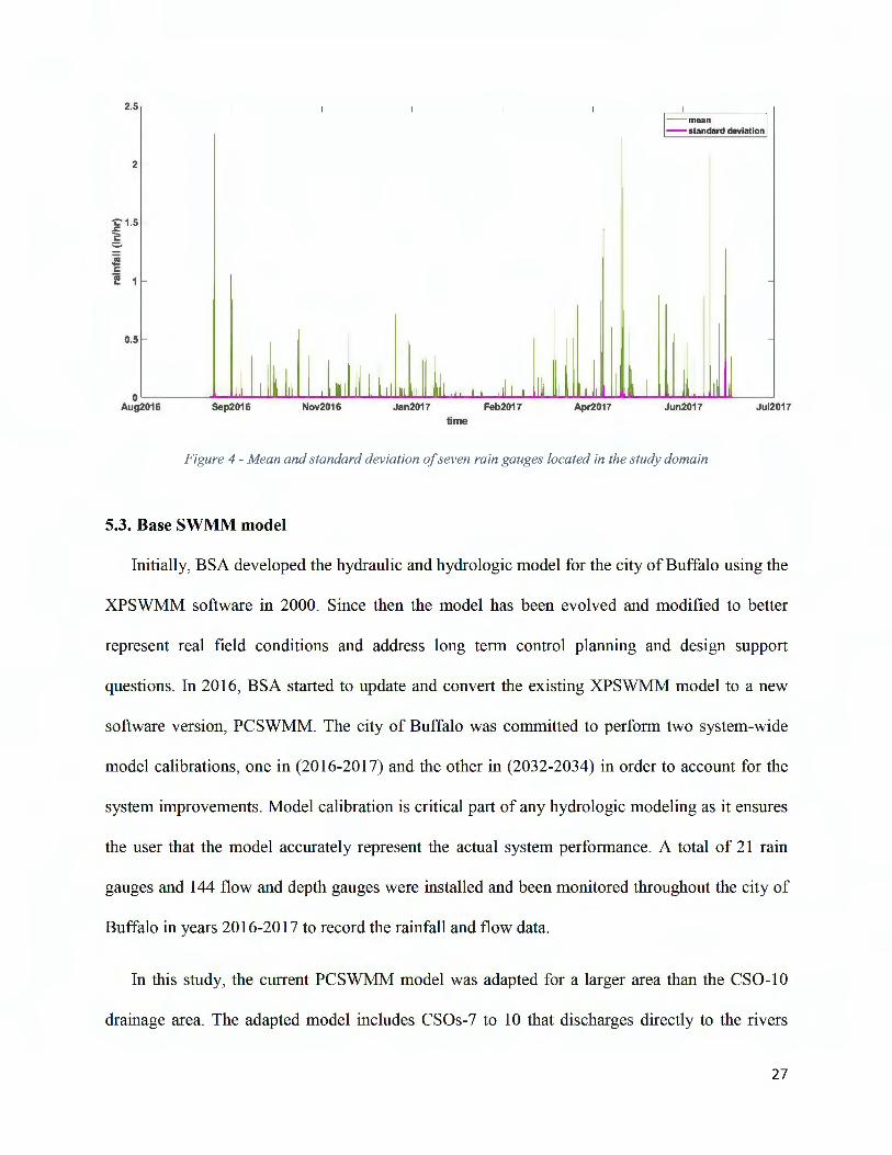
every 5-minutes from 9/15/2016 to 7/1/2017.

The precision of the rain gauges was set at 0.01 inch of rain. Figure 4 shows the mean and

standard deviation of seven rain gauges located in the study domain. As it is shown in this figure,

within the time period of9/15/2016 to 7/1/2017, spatial variation was quite small in this area except

for 6/27/2017. More frequent storms occurred in the second half of the period than the first half

5.2.2. Flow data

Flow meters were installed and collected depth and velocity of flows during both dry and wet

weather at different locations within the BSA system. Flow measurements were taken at 5-minute

intervals. For the CSO-10, data from flow meter named SJD _FM32t was used which is located at

the Breckenridge west of Niagara and monitored the inflow of SPP21 , where excess flow is

diverted to CSO-10 outfall (see figure 3). Figure 5 shows the observed flow data.

26

- mean - standard deviation

2

0.5

o~--- ~--~-~----- - - -~-~--- ---~~---- -~ Aug2016 Sep2016 Nov2016 Jan2017 Feb2017 Apr2017 Jun2017 Jul2017

time

Figure 4 - Mean and standard deviation ofseven rain gauges located in the study domain

5.3. Base SWMM model

Initially, BSA developed the hydraulic and hydro logic model for the city of Buffalo using the

XPSWMM software in 2000. Since then the model has been evolved and modified to better

represent real field conditions and address long term control planning and design support

questions. In 2016, BSA started to update and convert the existing XPSWMM model to a new

software version, PCSWMM. The city of Buffalo was committed to perform two system-wide

model calibrations, one in (2016-2017) and the other in (2032-2034) in order to account for the

system improvements. Model calibration is critical part of any hydrologic modeling as it ensures

the user that the model accurately represent the actual system performance. A total of 21 rain

gauges and 144 flow and depth gauges were installed and been monitored throughout the city of

Buffalo in years 2016-2017 to record the rainfall and flow data.

In this study, the current PCSWMM model was adapted for a larger area than the CSO-10

drainage area. The adapted model includes CSOs-7 to 10 that discharges directly to the rivers

27

during wet weather events and is divided into 686 different sub-catchments to represent the

catchments ' spatially distributed characteristics. The total number of conduits and nodes are 76

and 75 , respectively. Conduits can be in form of either pipes or channels that connect the drainage

system nodes to one another. Junction nodes and outfall nodes are part of the drainage network

that represent the confluence of surface channels, manholes, and terminal nodes of the drainage

system.

Three SWMM processes including Rainfall/Runoff, Groundwater, and Flow Routing were

applied in current research. The Green-Ampt method was used for infiltration estimates and flow

routing computations were based on the dynamic wave method. Daily evaporation values and

measured rainfall data were imported as input data to the SWMM model.

The base model has been manually calibrated, see figure 5. As shown in this figure, predictions

of the base model are in satisfactory agreement with the observed data. In current study, it was

assessed that whether the developed tool could further improve the performance of the manually

calibrated SWMM model.

45 Validation

40

35--Calibration

A 30 c., ~ 25-f:=.: 20

,S 15 i;..

• •

-

Observation

Base model

10

5

0 Aug-16 Oct-16 Nov-16 Jan-17 Mar-17 Api·-17 Jun-17 Aug-17

Time

Figure 5 - Observed and simulated flow data from manually calibrated base SWMM model for calibration and validation time periods.

28

5.4. Sensitivity analysis and variables

Prior to performing calibration, a sensitivity analysis was performed. In this study, Width,

Suction, Conduct, InitDef, Nperv, Nimperv, DSperv, Dsimperv, %Slope, Rough, %Imp,

¾Zerolmp were included in the sensitivity analysis as they are the most frequently reported

sensitive parameters in the literature (see Figure 1 ).

Manual sensitivity analysis was performed by changing the value of one parameter at a time

and comparing the changes in the simulated peak flow and average flow from the outputs. In order

to perform the sensitivity analysis, the limit or the range of the parameters should be identified

within which the parameters are perturbed. The indicated SWMM input parameters can be

categorized into four different groups based on uncertainty in estimating them (James 2003).

Categorization of the four different uncertainty classes 1s described hereunder:

Uncertainty class 1: Parameters can be measured and estimated with almost total certainty.

Uncertainty class 2: Parameters can be estimated with a high degree of certainty in the field or

laboratory.

Uncertainty class 3: Parameters cannot be easily measured in the field or laboratory.

Uncertainty class 4: Parameters cannot be measured with any certainty at all.

For the mentioned uncertainty classes, the recommended range of perturbation are (James

2003):

Uncertainty class 1: ± 5-10% Uncertainty class 2: ± 10-25%

Uncertainty class 3: ± 25-50% Uncertainty class 4: ± 50-100%

For each of the parameters included in the sensitivity analysis, the associated estimated

uncertainty class and the recommended range is shown in Table 3.

29

Table 3 - input parameters and their estimated uncertainty class

Input Estimated

parameter uncertainty class

Suction 3

Conduct 4

InitDef 4

Nperv 4

Nimperv 2

DSperv 4

Dsimperv 3

%Slope 2

Rough 2

%Imp 3

¾Zeroimp 2

Width 4

Recommended

perturbation range

±50%

±50%

±75%

±75%

±25%

±75%

±50%

±25%

±25%

±50%

±25%

±50%

peak flow

Max% change

0.007

3.160

1.610

0.006

2.230

8.570

0.010

1.480

9.470

11 .240

0.003

4.300

Rank

10

5

7

11

6

3

9

8

2

1

12

4

average flow

Max% change Rank

0.004 10

0.021 5

0.015 7

0.005 9

0.035 4

0.013 8

0.001 11

0.016 6

0.050 3

1.400 1

0.001 11

0.060 2

30

6. Results

6.1. Sensitivity Analysis

Assessment of the importance of the indicated 12 SWMM parameters on model outputs was

done by performing one-at-a-time sensitivity analysis. The maximum percent change in peak flow

and average flow for each parameter were identified and ranked, refer to Table 3, and the results

of the sensitivity analysis with respect to peak flow and average flow are presented in figure 6.

Figure 6 and table 3 show that the percent changes in peak flow are most sensitive to Rough,

DSperv, Nimperv, Width, Conduct, Nperv, and InitDef. The percent changes in average flow are

most sensitive to Nimperv, %Imp, Rough, and Width. Although %Slope was the sixth most

sensitive parameter in prediction of average flow, it was excluded from model calibration as the

study area was flat and it was assumed that the provided SWMM model by BSA could estimate

the %Slope with almost total certainty. Changes in all model parameters including, ¾Zeroimp,

Dsimperv, Nperv, and Suction were very small and insignificant; hence, theses parameters were

specified with a fixed value and excluded from model calibration.

6.2. Range of calibrated parameters

Initial results of automatic calibration have shown that the calibrated values for Nimperv and

%Imp were very close to the upper bounds of the parameters as defined in the section 4.3. As a

result, the bounds of the two parameters were modified in order to cover a broader range. The

modified bounds ofNimperv and %Imp were taken from Rossman, (2009) and Barco et al. (2008),

respectively. The perturbation range ofNimperv was from 0.01 mm to 0.2 mm (-33% to 1200%

of the initial value) and the perturbation range of %Imp was from 5% to 30% (-50% to 180% of

the initial value). ). It was assumed that each of the seven parameters were changing with the same

ratio for each subcatchment.

31

10 --<>- Suction --<>-Conduct -<>- I nitDef --<>- Nperv

5 --<>- Nimperv --<>- DSperv :;:

0 --<>- DSim perv .;::::

-<>-Width-"'-(1l 0 Q) -<>-%Slope a. -<>- Rough C

-<>-%ImpQ) CJ) -<>-%ZeroImpC (1l -5 .c u ~ 0

-10

-15 ~---~---~---~---~---~---~---~---~---~---~ -100 -60 -40 -20 0 20 40 60 80 100

% change in indicated parameters

a)

--<>- Suction 0.1 --<>- Conduct

--<>- lnitDef 0.05

__,,__ Nperv

0 --<>- Nimperv --osperv

:;: -0.05 --<>- DSimperv 0

__,,__ Width ~ -0.1 CJ) -<>- %Slope m -0 15 --Roughai .

-<>-%Imp/ti -0.2 C -<>- %Zero Imp

Q)

g> -1.2 (1l

-5 -1 .25 ~ 0

-1.3

-1.35

-1.4

-1.45

-1.5 ~---~----~---~----~----~---~----~----~---~ -80 -60 -40 -20 0 20 40 60 80 100

% Change in indicated parameters

b)

Figure 6 - Sensitivity analysis ofstudy domain with respect to a) peakflow and b) average flow

32

6.3. Single objective calibration

In single objective calibration, OSTRICH-SWMM was used to calibrate the SWMM model

using objective functions based on peak flow and average flow, Obj_ 1 and Obj_ 2, respectively.

The results of single automatic calibrations are shown in tables 4 and 5, respectively. As shown in

these tables, %Imp was a major calibrated parameter in calibration process using Obj_ 2; however,

it did not change in the calibration process using Obj_ 1. Nimperv was a major calibrated parameter

in calibrating using Obj_ 1 and the value of Nimperv increased; however, Nimperv value went to

the opposite direction and decreased in calibration using Obj_ 2. The value of InitDef also went to

different directions in both calibrations.

Tables 6 shows the results of single objective calibrations along with the observed flow and

the outputs of base model for the calibration time period. As expected, using the calibrated

parameters from the calibration process using Obj_ 1 yielded a better estimation ofpeak flow than

using the calibrated parameters from the calibration process using Obj_ 2. In addition, using the

calibrated parameters from the calibration process using Obj_ 2 yielded in better estimation of

average flow than using the calibrated parameters from the calibration process suing Obj_ 1.

For the validation time period, SWMM predictions were generated using the calibrated

models and are shown in Table 7. The base model performed better in terms of peak flow. Using

the calibrated parameters from the calibration using Obj_ 2 yielded in better estimation of average

flow; however, using the calibrated parameters from the calibration using Obj_ 1 yielded in the

worse estimation ofpeak flow. This indicates if automatic calibration tool is used but only includes

single objective, it may not work well. This is the limitation of single objective calibration and

shows automatic single objective calibration is not always good. This is due to the fact that there

are different combinations of parameters that result in the same value of output if only one

objective is evaluated.

33

Table 4- percentage ofchange in calibrated parameters from initial value andpercentage ofchange in peakflow from the base model.

Input parameter Percent change from initial value Percent change in peak flow

Rough -4.5% +0.6%

Nimperv +130% -9%

%Imp +4% 0

Conduct -25% 0

DSperv +75% 0

InitDef -65% +1%

Width +40% +2 .3%

Table 5- percentage ofchange in calibrated parameters from initial value and percentage ofchange in average flow from the base model.

Input parameter Percent change from initial value Percent change in average flow

Rough -10% +0.02%

Nimperv -20% +0.028%

%Imp +200% +0.384%

Conduct +25% +0.009%

DSperv +20% -0.006%

InitDef +75% +0.011%

Width +45% +0.04%

Table 6 - Model outputs and error values ofsingle objective calibration and base model along with the observed data for calibration time period.

Model outputs Errors

Peak flow Average flow Peak flow Average flow

value (MGD) value (MGD) error (MGD) error (MGD)

Observed value 28 .9 1.250

Base SWMM model 30.4 1.225 1.5 -0.025

Peak flow 28.9 1.224 0.0 -0.026

Average flow 32.9 1.232 4.0 -0.018

34

Table 7 - Model outputs and error values ofsingle objective calibration and base model along with the observed data for validation time period.

Model outputs Errors

Peak flow Average flow Peak flow Average flow

value (MGD) value (MGD) error (MGD) error (MGD)

Observed value 37.9 1.477

Base SWMM model 37.8 1.396 -0.1 -0.081

Peak flow 35.2 1.394 -2 .7 -0.083

Average flow 39.4 1.402 1.5 -0.075

6.4. Multi-objective calibration including peak flow and average flow

Due to the limitation of single objective calibrations, multi-objective calibration was

performed by considering both Obj_ 1 and Obj_ 2. First, ObjectiveFunction was set to GCOP and

the resulted Pareto front curve as well as the results of single objective calibrations are shown in

figure 7. The best solution for each objective was obtained when only one objective function was

considered for calibration. The best solutions for peak flow and average flow are shown in figure

7 by pink and orange points, respectively. In the calibration process using Obj_ 1, average flow

gets worse and in the calibration process using Obj_ 2, peak flow gets worse, see table 6 and figure

7. According to figure 7, the solutions to the multi-objective problem consists of the sets of

solutions with trade-offs between the conflicting objective functions considered in the calibration

process and there is no single solution that satisfies both objectives. , there exists a number of

Pareto optimal solutions, also called non-dominated solutions, in which one objective function

improves with degradation of the other objective function. The set of Pareto optimal solutions is

often called the Pareto front that consists of the set of optimal solutions. Without additional

subjective preferences, all Pareto optimal solutions are considered equally good.

In order to select a point from the Pareto front, a criterion must be defined. In current study,

ObjectiveFunction was set to WSSE which results in only one set of parameter. The results of

35

multi-objective automatic calibrations by using WSSE are shown in table 8. As shown in this table,

Nimperv increased by+125% from its initial value since it was the most important parameter in

calibration using Obj_ 1. The percent change was less than + 130% as it was in calibration using

Obj_1. This is due to the fact that Nimperv was decreasing when calibrating using Obj_2.

Increasing Nimperv had a negative impact on average flow. The value of %Imp was the same as

it was in single objective calibration using objective function based on average flow because it is

not an important parameter in single objective calibration using objective function based on peak

flow.

Tables 9 and 10 show the results of single and multi-objective calibrations as well as the

observed flow and the outputs of base model for the calibration and validation time periods,

respectively. As shown in tables 9 and 10, the values of the outputs from the multi-objective

function are generally within the range of the outputs from the single objective calibrations and

multi-objective calibrations performed better than the base model and any of the two single

objective calibrations.

Single objective calibration emphasize certain aspects of flow ( e.g. , peak flow or average

flow) and simulate the other aspects of flow with less accuracy. This is due to the fact that there

exist conflicts between the different objective functions , improvements in either one of the

objectives deteriorated the model performance in terms of the others. No single calibration can

meet the needs of all modeling applications. When more objective functions were included in the

calibration process, the sets of optimal solutions and the performance of the calibrated model also

differed. Compared to the observed flow data, all of the multi-objective functions performed better

than the single objective calibrations as they take into account two or more aspects of flow.

36

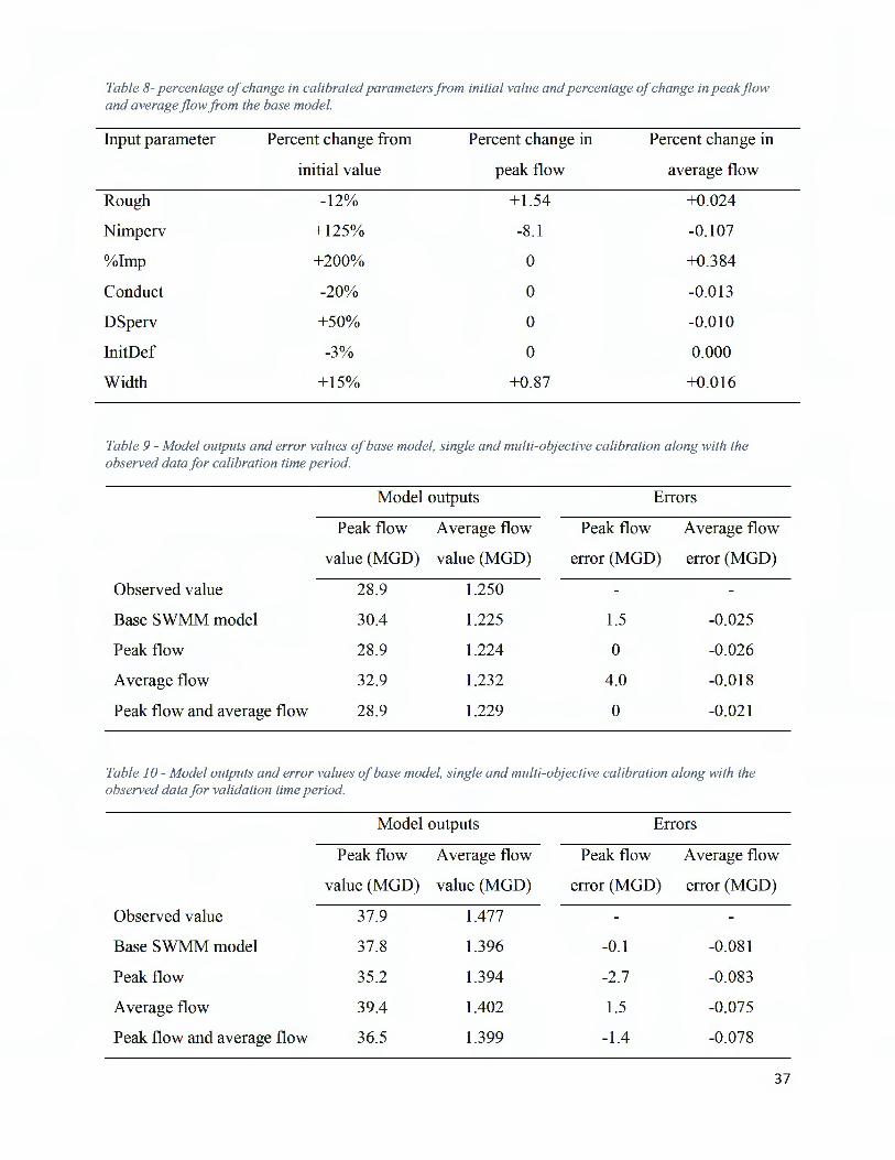
Table 8- percentage ofchange in calibrated parameters from initial value and percentage ofchange in peakflow and average flow from the base model.

Input parameter Percent change from Percent change in Percent change in

initial value peak flow average flow

Rough -12% +1.54 +0.024

Nimperv +125% -8 .1 -0.107

%Imp +200% 0 +0.384

Conduct -20% 0 -0.013

DSperv +50% 0 -0.010

InitDef -3% 0 0.000

Width +15% +0.87 +0.016

Table 9 - Model outputs and error values ofbase model, single and multi-objective calibration along with the observed data for calibration time period.

Model outputs Errors

Peak flow Average flow Peak flow Average flow

value (MGD) value (MGD) error (MGD) error (MGD)

Observed value 28 .9 1.250

Base SWMM model 30.4 1.225 1.5 -0.025

Peak flow 28.9 1.224 0 -0.026

Average flow 32.9 1.232 4.0 -0.018

Peak flow and average flow 28 .9 1.229 0 -0.021

Table 10 - Model outputs and error values ofbase model, single and multi-objective calibration along with the observed data for validation time period.

Model outputs Errors

Peak flow Average flow Peak flow Average flow

value (MGD) value (MGD) error (MGD) error (MGD)

Observed value 37.9 1.477

Base SWMM model 37.8 1.396 -0.1 -0.081

Peak flow 35 .2 1.394 -2 .7 -0.083

Average flow 39.4 1.402 1.5 -0.075

Peak flow and average flow 36.5 1.399 -1.4 -0.078

37

10 o dominated solutions

9 _._ non-dominated solutions

- + solution of single objective with respect to average fl ow + solution of single objective with respect to peak fl ow0 8

(!) 0

0 0 00 ~ 07 0 0:s: 0

0-= ~ 6

0

0 0

Q) 0 Ctl

<l) 0 a. 5 0C:

0 0 L. 000

0 0L. 4 0 0

Q) 0 L.

Q) 0 0

0 0 0:J 3 0 0

0 00 0CJ) ..Cl 8 'b O 0

Ctl 02 0 8 ,l ~

00Ooo o 0 0

06) 0 O 0 0 O 0 0 0 O O 0

0 00 '--------------------'-----ll......- - - - - --~--------'--------------------'

0.015 0.02 0.025 0.03

absolute error in average flow (MGD)

Figure 7- set ofPareto optimal solutions for a two-objective calibration including, peakflow and average flow. The single objective solutions were also shown by pink and orange points.

6.5. Multi-objective calibration with consideration of time series of flow data

Objective functions considered in previous sections, Obj_ 1 and Obj_ 2, do not take advantage

of all of the observation data that are available. Furthermore, two totally different hydro graphs can

result in the same values of peak flow or average flow. Hence, Obj_3 was added as one of the

objective functions that takes into account all of the observations in time series of flow data.

Two multi-objective calibrations were performed. The first one considered Obj_ 1 and Obj_3

as objectives and later considered Obj_ 2 and Obj_3 as objectives. The non-dominated and

dominated solutions for corresponding multi-objective calibration were shown in figures 8 and 9,

respectively. These figures show that model predictions using the calibrated parameters of single

objective calibration could result in estimations of other objectives with less accuracy.

38

The size and shape of the Pareto surfaces obtained indicate the correlation between different

objectives (Khu and Madsen 2005). According to this statement, Obj_ 1 and Obj_3 are more

correlated with each other than both Obj_l and Obj_2, and Obj_2 and Obj_3 (see figures 7, 8, 9).

0.33 I I I I I

0 dominated solutions ...... non-dominated solutions

co 0.32 + solution of single objective with respect to average flow -

ro -0

0 0 + solution of single objective with respect to peak flow -:!:2 0.31 -- ' 0

@ ♦ 0

-

0 CJ) Q)

-~ -0.3

0 0

0 -

CJ) 0 0 0 0

Q)

.§ 0.29 -Q)

£ 0

0

0

6'

0

00 0

0

0

0

0 0

0 0

-

.£ 0.28 -0

0 -w

◄(/)

~ p!j c::: 0.27 - 4

0

0 ~ 0 0

~ j'~ cf] 'boif> o

0

0

o

0

0 It,

0

-

I I I I I I I I I0.26

0 2 3 4 5 6 7 8 9 10

absolute error in peak flow (MGD)

Figure 8 - set ofPareto optimal solutions for a two-objective calibration including, peakflow and RMSE. The single objective solution with respect to peakflow and average flow were shown by pink and orange points, respectively.

0 o dominated solutions ...... non-dominated solutions

0.33 co + solution of single objective with respect to peak flow ro + solution of single objective with respect to average flow-0

:!: 0.32 0

0 0.;:::- 0 0 0

Q) ~ 0.31 ♦ (b

0 -~ 0

0~ 0.3 0 0

0E 0

.:,

£Q)

0.29 0 0 0

0 L.

$ 0 0

0 ~ 0.28 0

O O O O O 0 ♦0~ 0 ~ 0 oo O 0

0c::: 0 ~ Oo Oc900 oO ~ 0.27

0.26 ~--~---~--~---~--~---~---~--~---~--~--~ 0.017 0.018 0.019 0.02 0.021 0.022 0.023 0.024 0.025 0.026 0.027 0.028

absolute error in average flow (MGD)

Figure 9 - set ofPareto optimal solutions for a two-objective calibration including, average flow and RMSE. The single objective solution with respect to average flow and peak flow were shown by orange and pink points, respectively.

39

Table 11 shows the model outputs of all combinations of multi-objective automatic

calibrations as well as the base SWMM model and observed data. Table 12 also shows the

deviation of all multi-objective calibration and base model from the observations for calibration

time period. As shown in this table, among the multi-objective calibrations, the one including

Obj_ 1 and Obj_ 2 performed better compared to others.

For the validation time period, model outputs ofmulti-objective calibrations including, Obj_ 1

and Obj_2 and Obj_l , Obj_2, and Obj_3 were shown in table 13 and their deviations from

observation are shown in table 14. As shown in these tables, multi-objective calibration including

the three objectives performed better. This indicates that by including more aspects of flow as

objective functions, the simulated SWMM model is steadier and more reliable.

These findings indicate that although single objective calibration performs better for

calibration time period when only one objective is considered, multi-objective calibration performs

better for validation time period.

Model validation is a necessary and integral part of any calibration effort since calibrated

models are normally used in forecasting. So implementing multi-objective calibration is

recommended for calibration as it takes into account more aspects of flow compared to single

objective calibration that only considers one. Multi-objective calibration minimizes the possibility

of equifinality which is a drawback in single objective calibration and provides a model which is

closer to the reality.

40

Table 11- Model outputs for base model, multi-objective calibrations, and observed data for calibration time period

Peak flow Average flow RMSE

(MGD) (MGD)

Observed value 28 .9 1.250

Base SWMM model 30.4 1.225 0.283

Peak flow and average flow 28 .9 1.229 0.278

Peak flow and time series of flow data 28 .6 1.226 0.286

Average flow and time series of flow data 28 .3 1.228 0.273

Peak flow, average flow, and time series of flow data 26.9 1.229 0.272

Table 12 - Deviation ofmulti-objective calibrations and base model from the observed data for calibration time period

Peak flow Average flow RMSE

error error (MGD)

(MGD)

Base SWMM model 1.5 -0.025 0.283

Peak flow and average flow 0.0 -0.021 0.278

Peak flow and time series of flow data 0.3 -0.024 0.286

Average flow and time series of flow data 0.6 -0.022 0.273

Peak flow, average flow, and time series of flow data 1.1 -0.026 0.272

Table 13 - Model outputs for base model, multi-objective calibrations, and observed data for validation time period

Peak flow Average RMSE

(MGD) flow (MGD)

Observed value 37.9 1.477

Base SWMM model 37.8 1.396 0.458

Peak flow and average flow 36.5 1.399 0.456

Peak flow, average flow, and time series of flow data 38.9 1.393 0.445

41

Table 14 - Deviation ofmulti-objective calibrations and base model from the observed data for validation time period

Peak flow Average RMSE

error flow error

(MGD) (MGD)

Base SWMM model -0.1 -0.081 0.458

Peak flow and average flow -1.4 -0.078 0.456

Peak flow, average flow, and time series of flow data 1.0 -0.084 0.445

42

6.6. Goodness of fit measures

Besides RMSE, other goodness of fit measures can also be used to evaluate the performance

of single and multi-objective calibrations. Therefore, three other goodness of fit statistics

parameters including, Nash-Sutcliffe Efficiency (NSE), Percent Bias (PBIAS), and ratio of the

root mean square error to the standard deviation of measured data (RSR) were used which have

been recommended by Moriasi et al. (2007). For each calibration included in table 9 and 11 ,

predicted flow was plotted versus observed flow and NSE, PBIAS, and RSR were calculated, see

figure 10. The line ofequality, where predicted and observed flow are exactly the same was shown

by dashed line in each plot. This is a line through passes through the origin at 45 degrees to the

axes.

In figure 10, all PBIAS values are positive that indicates the calibrated models were

underestimating the flow which is consistent with the results shown in tables 9 and 11. In these

tables, all of the simulated average flow is less than the observed average flow. Calibrated model

including Obj_ 2, (b) in figure 10, has the smallest PBIAS value as expected compared to other

calibrated models. RSR is calculated as the ratio of the RMSE and standard deviation ofmeasured

data and it is the smallest when one of the objectives is Obj_23 , (f) and (g).

43

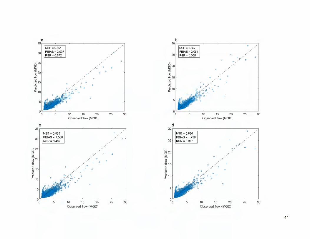
a 35 1 /

NSE = 0.861 / /

PBIAS = 2.007 ;>/ /

30 RSR = 0.372 /

/

11 / /

/ 0

025 / /

CJ / /

/ 0 8 ~ / 0

---;20 /

,4' 0

0 /0:: / 0/-a

0 0 / ~ 15 /

/ 0

'o 0 // 0 0

e! 0 / O 0

o_ 10 9 / ic& O Oo

~o 0

5

0 0 5 10 15 20 25 30

Observed flow (MGD)

C 35 ~--~--~--~---~--~--~

/

NSE = 0.835 0 /

/

30 PBIAS = 1.568 /

/ / 0

RSR = 0.407 / /

/ /

/ /~25

/0 CJ

/ /

/ 0 0

~ / / 0~20

/

0~ / /

0 0

0:: // 0-a 0

02 15 // /

00u 'o / 0

0 o ,,, / a e! o_ 10 0 8.,. ~ ,,, o go o o o

00 06' O 0 0

0 0

0 §5

o ~--~--~--~---~--~--~ 0 5 10 15 20 25 30

Observed flow (MGD)

b 30~--~ --~ ---~ --~ --~ --~

NSE = 0.867 0

/ /

/

PBIAS = 2.064 / /

25 RSR = 0.365 / /

0 / 0

0 :/

0 / §

/0 /

/

CJ 20 / /

/ /

/

~ / 0

o:: 15 0 / /

~ 0

-a 0 // 0 0

<l)

ti 0 /

'o 0 / / 0

0 / 0£ 10 / 0 c.i 0

0

6' 0 0

00 0

5

o~--~ --~ ---~ --~ --~ --~ 0 5 10 15 20 25 30

Observed flow (MGD)

d 30 ~--~--~---~--~--~--~

/0

NSE = 0.866 / /

/ /PBIAS = 1.750

0 /25 RSR = 0.366 /

/

? / 0 ~ 0

0 / 0 /0 /CJ 20 /

~ / 0 /

/

~ /

/ 02 15 0 /

/

/-a / 0

~ 0 0 // 0

'o 08 4' 0e! 10 0 / 0 o_ / O r.i 0

<>' 0 0

00 0

5

0 0 5 10 15 20 25 30

Observed flow (MGD)

44

0

e f 30 ~--~--~---~--~--~--~30 1,--

/ /NSE = 0.858 0

0 /

/

NSE = 0.871 0 /

/

0

PBIAS = 1.956 0 0 /

/

PBIAS = 1.774 / /

0 / /

25 1 RSR = 0.376 / / 25 RSR = 0.360 /

/

1 / 0 /

/ 0 /0 / 0 / 0 0 0

0 / /

0 6' o820 / / 0

0 20 /

/

~ / /

~ /

~ / / / /0 0

/ ~ / 0_g 15 /

/

0 s::: 15 /

/

-c, 0 / 0 -c, 0 / Q) / / 0

t5 / /

0 /

0 -~ 0 0 ,,,,,, 0 0 / 0 -c,

o ,,,o o0 / /0 Oo 0

'6 ~ 10 ct 10 o o_,,,,, o o o a.. / 0 Cf'l

0 $ 0 <:.i 0 &'. 0 - \, 0

@.:, 00

5 5

0 o------~---~-----~---0 5 10 15 20 25 30 o 5 10 15 20 25 30

Observed flow (MGD) Observed flow (MGD)

g 30

/

NSE = 0.871 0 / /

PBIAS = 2.153 /

/

25 1 RSR = 0.358 / /

/

~ 'o1/

0 / !l 0 /

/820 / 0 /~ /

/ 0 /~ /

/s::: 0

15 / 0 -c, / Q) 0 / 0

0t5 0 /

/

'6 0 // o

~ 10 a..

5

5 10 15 20 25 30 Observed flow (MGD)

Figure JO - predicted versus observedflow for a) base model, calibration considering b) Obj_], c) Obj_2, d) Obj_] and Obj_2, e) Obj_] and Obj_3, j) Obj_2 and Obj_3, g) Obj_], Obj_2, and Obj_3. Line ofequality is shown by dot in each one.

45

7. Discussion

In current study, sensitivity analysis was performed manually and OSTRICH-SWMM was

used for automated calibration. In fact, OSTRICH can also be used for automated sensitivity

analysis by implementing three parameter sensitivity measures including Dimensionless Scaled

Sensitivities (DSS), Composite Scaled Sensitivities (CSS), and One-percent Scaled Sensitivities

(1 ¾SS) which is not the focus of this study. Future work can focus on using OSTRICH-SWMM

for sensitivity analysis and compare the results with this study.

There are two different algorithms available within OSTRICH that are suited for multi­

objective calibration purposes including, P ADDS and SMOOTH. In this case study, parallelized

version of the P ADDS algorithm (ParaP ADDS) was faster and more efficient in reaching the

optimal point compared to SMOOTH. Adding other types of algorithms, such as NSGAII which

was used most often in literature, and implementing them for automated calibration will help to

propose the best optimization algorithm for calibration of SWMM models.

In this study, multi-response modes were used in multi-objective calibration. Multi-variable

measurements, such as flow and depth, and multi-site measurements can also be implemented in

multi-objective calibration to further improve the SWMM models.

Our observation values were taken every 5-min, if they were taken at other time steps, the

calibrated model would behave differently since the value of the observations (e.g. , peak flow)

may change.

To Authors ' best ofknowledge, none ofthe previous studies have included time delay analysis

in their studies. Without considering time lag in calibration process, calibration may result in a

parameter set that perfectly capture every aspect of flow such as peak flow or average flow except

RMSE. Figure 11 shows an example of such situation. As shown in this figure, the simulated peak

46

flow and average flow are close to the observed values; however, there is a time lag between

simulated and observed flow. Future work will focus on using the statistics measures such as cross­

correlation to consider time lag in multi-objective calibrations.

Last but not least, OSTRICH-SWMM should be used for different types ofland uses and rain

patterns to conclude about in which cases, modeling conflicts between peak flow, average flow,

and time series of flow data exist.

40 ~-------~~-------~--------~--------~ - - single objective calibration with respect to peak flow - observed - - base model 35 - - multi-objective calibration

30

15

10

5 ~--------~--------~---------~-------~ 17:00 17:30 18:00 18:30 19:00

Time Apr20 , 2017

Figure 11 - An example to highlight the importance oftime delay analysis.

47

8. Summary and Conclusion

• The results of sensitivity analysis reveals that the percent changes in peak flow are most

sensitive to Rough, DSperv, Nimperv, Width, Conduct, Nperv, and InitDef. The percent

changes in average flow are most sensitive to Nimperv, %Imp, Rough, and Width. Changes in

all model parameters including ¾Zerolmp, %Slope, Dsimperv, Nperv, and Suction were very

small and insignificant; hence, were assumed to be constant.

• OSTRICH-SWMM is an open source tool that proved to be useful for automatic calibration of

SWMM models. It is capable of being used not only for event based calibrations but also for

continuous calibrations which is not often considered in literature.

• Model validation is a necessary and integral part of any calibration effort since calibrated

models are normally used in forecasting. A comparison of single and multi-objective

calibration performance indicates multi-objective calibration results in a more robust

parameter set than any single objectives.

• Multi-objective calibration is recommended for calibration of hydrological models.

• Due to the existence of conflicts between different objectives, a Pareto front was obtained that

provides optimal solutions. Based on the defined criteria, an optimal solution can be selected

from the obtained Pareto front.

• This study highlight the importance of determining and considering time delay between

simulated and observed values in model calibration problems.

48

9. References

1. Abrishamchi, A. , A. Massoudieh, and M. Kayhanian (2010). "Probabilistic modeling of

detention basins for highway storm water runoff pollutant removal efficiency." Urban

Water Journal 7(6): 357-366.

2. Akan, A. 0. , and R. J. Houghtalen (2003). "Urban hydrology, hydraulics, and stormwater

quality: Engineering applications and computer modeling." Wiley, Hoboken, NJ.

3. Alamdari, N . (2016). "Development of a robust automated tool for calibrating a SWMM

watershed model." In Proceedings of the World Environmental and Water Resources

Congress, West Palm Beach, FL, 221-228 .

4. Aubert, D. , C. Loumagne, and L. Oudin (2003). "Sequential assimilation of soil moisture

and streamflow data in a conceptual rainfall-runoff model." Journal of Hydrology 280:

145-161.

5. Baek, S.-S ., D.-H. Choi, J.-W. Jung, H.-J. Lee, H. Lee, K.-S. Yoon and K. H. Cho (2015).

"Optimizing low impact development (LID) for stormwater runoff treatment in urban area,

Korea: Experimental and modeling approach." Water Research 86: 122-131.

6. Balascio, C. C., D. J. Palmeri and H. Gao (1998). "Use of a genetic algorithm and multi­

objective programming for calibration of a hydrologic model." Transactions of the ASAE

41(3): 615-619.

7. Barco, J. , K. M. Wong and M. K. Stenstrom (2008). "Automatic calibration of the U.S.

EPA SWMM model for a large urban catchment." Journal of Hydraulic Engineering

134(4): 466-474.

8. Bartelt-Hunt, S. L. , T. B. Culver, J. A. Smith, L. S. Matott, A. J. Rabideau (2006). "Optimal

Design of a Compacted Soil Liner Containing Sorptive Amendments." Journal of

Environmental Engineering 132: 769-776.

9. Beling, F. A. , J. I. B. Garcia, E. M. C. D. Paiva, G. A. P. Bastos, and J.B. D. Paiva (2011).

"Analysis of the SWMM model parameters for runoff evaluation in Periurban basins from

Southern Brazil." 12nd International Conference on Urban Drainage, Porto Alegre/ Brazil,

11-16.

10. Beven, K. , and A. Binley (1992). "The future of distributed models: Model calibration and

uncertainty prediction." Hydrological Processes 6(3): 279-298.

11. Blumensaat, F. , M. Wolfram and P. Krebs (2012). "Sewer model development under

minimum data requirements ." Environmental Earth Sciences 65(5): 1427-1437.

49

12. Borris, M. , G. Leonhardt, J. Marsalek, H. Osterlund and M. Viklander (2016). "Source­

based modeling of urban stormwater quality response to the selected scenarios combining

future changes in climate and socio-economic factors ." Environmental Management 58(2):

223-237.

13 . Box, M.J. (1965). "A new method ofconstrained optimization and a comparison with other

method." Computer Journal 8(1) : 42-52.

14. Brocca, L., F. Melone, T. Moramarco, W. Wagner, V . Naeimi, Z. Bartalis, and S.

Hasenauer (2010). "Improving runoff prediction through the assimilation of the ASCAT

soil moisture product" Hydrology and Earth System Sciences 14(10): 1881-1893.

15 . Burszta-Adamiak, E. and M. Mrowiec (2013) . "Modelling of green roofs hydrologic

performance using EPA's SWMM." Water Science and Technology 68(1): 36.

16. Carvalho, M., K. M. T. Formiga, and E. Q. Siqueira (2011). "Calibration ofUrban Drainage

12thModels with Multiobjective Evolutionary Algorithms." Proceedings of the

International Conference on Urban Drainage, Porto Alegre, Brazil, 11-16.

17. Cermola, J. A., H. M. El-Baroudi, D. R. Sachdev and S. DeCarli (1979) . "SWMM

Application to Combined Sewerage in New Haven." Journal of the Environmental

Engineering Division 105(6): 1035 - 1048.

18. Chen, J., and BJ. Adams (2006) . "Analytical urban storm water quality models based on

pollutant buildup and washoffprocesses ." Journal of Environmental Engineering 132(10):

1314-1330.

19. Chow, M. F., Z. Yusop and M. E. Toriman (2012) . "Modelling runoff quantity and quality

in tropical urban catchments using Storm Water Management Model." International

Journal of Environmental Science and Technology 9(4): 737-748 .

20. Chung, E.-S ., W.-P. Hong, K. S. Lee and S. J. Burian (2011). "Integrated use of a

continuous simulation model and multi-attribute decision-making for ranking urban

watershed management alternatives." Water Resources Management 25(2): 641-659.

21. Cooper, V.A. , V . T.V. Nguyen and J.A. Nicell (2007). "Calibration of conceptual rainfall­

runoffmodels using global optimization methods with hydro logic process-based parameter

constraints ." Journal of Hydrology 334: 455-466.

22 . Danish Hydraulic Institute (1995) . Mouse: User's manual and tutorial, Horsholm,

Denmark.

50

23. Del Giudice, G. and R. Padulano (2016). "Sensitivity analysis and calibration of a rainfall­

runoff model with the combined Use of EPA-SWMM and genetic algorithm." Acta

Geophysica 64(5): 1755-1778.

24. Dent, S. , R. B. Hanna, and L. Wright (2004). "Automated calibration using optimization

techniques with SWMM RUNOFF". Innovative modeling of urban storm water systems,

W. James, ed. , CHI, Inc. , Guelph, ON, Canada, 385-408.

25. Duan, Q. , S. Sorooshian, and V. K. Gupta (1994). "Optimal use of the SCE-UA global

optimization method for calibrating watershed models ." Journal of Hydrology 158 (3-4) :

265-284.

26. Fang, T. and J. Ball (2007). "Evaluation of spatially variable control parameters in a

complex catchment modelling system: a genetic algorithm application." Joumal of

Hydroinformatics 9(3): 163-173.

27. Fioretti, R. , A. Palla, L. G. Lanza and P. Principi (2010). "Green roof energy and water

related performance in the Mediterranean climate." Building and Environment 45(8):

1890-1904.

28. Freni, G. and G. Mannina (2012). "The identifiability analysis for setting up measuring

campaigns in integrated water quality modelling." Physics and Chemistry of the Earth 42 :

52-60.

29. Gallagher, M. , and J. Doherty (2007). "Parameter estimation and uncertainty analysis for

a watershed model." Environmental Modelling Software 22(7): 1000-1020.

30. Gaume, E. , J.-P. Villeneuve, and M. Desbordes (1998). "Uncertainty assessment and

analysis of the calibrated parameter values of an urban storm water quality model." J oumal

of Hydrology 210 (1-4): 38-50.

31. Goldberg, D. E. (1989). "Genetic Algorithms m Search, Optimization and Machine

Leaming." Addison-Wesley, Reading, MA.

32. Green, W. H. , and G. Ampt (1911). "Studies on soil physics. 1: The flow of air and water

through soils." Journal of Agricultural Science 4(1 ): 1-24.

33. Guin J. A. (1968). "Modification of the Complex method of constraint optimization"

Computer Journal 10: 416-417.

34. Giilbaz, S. and C. M. Kazezy1lmaz-Alhan (2013). "Calibrated hydrodynamic model for

sazlidere watershed in Istanbul and investigation of urbanization Effects." Journal of

Hydrologic Engineering 18(1): 75-84.

51

35. Haghnegahdar, A. , B. Tolson, B. Davison, F. Seglenieks, E. Klyszejko, E. D. Soulis, V.

Fortin, L. S. Matott (2014). "Calibrating Environment Canada' s MESH Modelling System

over the Great Lakes Basin." Atmosphere-Ocean 52(4): 281-293.

36. Helton, J.C. and F.J. Davis (2002). "Illustration of sampling-based methods for uncertainty

and sensitivity analysis." Risk Analysis 22: 591-622.

37. Herrera, M. , I. Heathcote, W. James and A. Bradford (2006). "Multi-Objective Calibration

of SWMM for Improved Simulation of the Hydrologic Regime." Journal of Water

Management Modeling R225-15. doi: 10.14796/JWMM.R225-15 (Formerly in Intelligent

Modeling of Urban Water Systems. ISBN: 0-9736716-2-9).

38. Horton, R. E. (1940). "The infiltration-theory of surface-runoff" Eos Transactions

American Geophysical Union 21(2): 541.

39. HR Wallingford Ltd (1997). Hydro Works on-line manual, Wallingford, U.K.

40. Hsu, M. H. , S. H. Chen and T. J. Chang (2000). "Inundation simulation for urban drainage

basin with storm sewer system." Journal of Hydrology 234(1): 21-37.

41. Huber, W. C. and R.E. Dickinson (1988). "Storm water management model user 's

manual" , version 4, EPA/600/3-88/00la (NTIS PB88- 236641/AS), Environmental

Protection Agency, Athens, Ga.

42. Jakeman, A.J. , R.A. Letcher, and J.P. Norton (2006). "Ten iterative steps in development

and evaluation of environmental models." Environmental Modeling Software 21 ( 5): 602-

614.

43. James, W. and A. Kuch (1998). "Sensitivity-calibration decision-support tools for

continuous SWMM modeling: a fuzzy-logic approach." Journal of Water Management

Modeling R200-09. doi: 10.14 796/JWMM.R200-09.

44. James, W. (2002). Rules for Responsible Modeling. Third Edition. CHI Publications.

45. James, W. , C. Robert, B. Wan, and W. James (2002). "Implementation in PCSWMM using

genetic algorithms for auto calibration and design-optimization." Proceedings of the 9th

International Conference on Urban Drainage - Global Solutions for Urban Drainage,

ASCE, Reston, VA, 1-10.

46. Johnston, J.M. , D. J. McGarvey, M. C. Barber, G. Laniak, J. Babendreier, R. Parmar, K.

Wolfe, S. R. Kraemer, M. Cyterski, C. Knightes, B. Rashleigh, L. Suarez, R. Ambrose

(2011). "An integrated modeling framework for performing environmental assessments:

52

Application to ecosystem services in the Albemarle-Pamlico basins (NC and VA, USA)."

Ecological Modelling 222(14): 2471-2484.

47. Kennedy, J., R. C. Eberhardt, Y. Shi (2001). "Swarm Intelligence." Morgan Kaufmann,

San Francisco (CA).

48 . Khu, S.T., and H. Madsen (2005). "Multi-objective calibration with Pareto preference

ordening: An application rainfall-runoff model calibration." Water Resources Research 41 .

W03004, doi: 10.1029/2004WR003041.

49. Knighton, J., E. Lennon, L. Bastidas, and E. White (2016). "Stormwater Detention System

Parameter Sensitivity and Uncertainty Analysis Using SWMM." Journal of Hydrologic

Engineering 21(8): 05016014.

50. Krebs, G., T. Kokkonen, M. Valtanen, H. Koivusalo and H. Setala (2013). "A high

resolution application of a stormwater management model (SWMM) using genetic

parameter optimization." Urban Water Joumal 10(6): 394-410.

51. Krebs, G., T. Kokkonen, M. Valtanen, H. Setala and H. Koivusalo (2014). "Spatial

resolution considerations for urban hydrological modelling." Journal of Hydrology 512:

482-497.

52. Lei, J. and W. Schilling (1994) . "Parameter uncertainty propagation analysis for urban

rainfall runoff modelling." Water Science and Technology 29(1-2): 145 .

53 . Li, C., W. Wang, J. Xiong, and P. Chen (2014). "Sensitivity analysis for urban drainage

modeling using mutual information." Entropy 16: 5738-5752.

54. Liong, S-Y. , W. T. Chan, and C. L. Law (1993) . "Computer-aided catchment-calibration

model." Advances in Engineering Software 17(3): 147-154.

55 . Liong, S-Y. , W. T. Chan, and J. ShreeRam (1995) . "Peak-flow forecasting with genetic

algorithm and SWMM." Journal of Hydraulic Engineering 121(8): 613-617.

56. Mailhot, A. , E. Gaume, and J. P. Villeneuve (1997). "Uncertainty analysis of calibrated

parameter values of an urban storm water quality model using metropolic Monte Carlo

algorithm." Water Science and Technology 36(5): 141-148.

57. Mancipe-Munoz, N .A. , S.G. Buchberger, and M.T. Suidan (2011). "Calibration of

distributed rainfall-runoff model in Hamilton County, Ohio." In: On Modeling Urban

Water Systems, CHI Press, Toronto, 177-191.

53

58. Mancipe-Munoz, N. A. , S. G. Buchberger, M. T. Suidan and T. Lu (2014). "Calibration of

rainfall-runoff model in urban watersheds for stormwater management assessment."

Journal of Water Resources Planning and Management 140(6): 05014001.

59. Matott, L. S., S. L. Bartelt-Hunt, A. J. Rabideau, and K. R. Fowler (2006a) . "Application

of Heuristic Optimization Techniques and Algorithm Tuning to Multilayered Sorptive

Barrier Design." Environmental Science & Technology 40(20): 6354-6360 .

60. Matott, L. S., A. J. Rabideau, and J. R. Craig (2006b ). "Pump-and-treat optimization using

analytic element method flow models." Advances in Water Resources 29: 760-775 .

61. Matott, L. S. , K. Leung, and J. Sim (2011). "Application of MATLAB and Python

optimizers to two case studies involving groundwater flow and contaminant transport

modeling." Computers & Geosciences 37(11): 1894-1899.

62 . Matott, L. S., B. A. Tolson, and M. Asadzadeh (2012). "A benchmarking framework for

simulation-based optimization of environmental models." Environmental Modelling &

Software 35 : 19-30.

63 . Matott L. S. (2016). "OSTRICH - An Optimization Software Toolkit for Research

Involving Computational Heuristics: Documentation and User 's Guide."

64. Matott, L. S. (2017). "Ostrich: an Optimization Software Tool, Documentation and User 's

Guide" , Version 17.10.18. University at Buffalo, Center for Computational Research,

Buffalo, NY.

65 . McKay, M., R. Beckman, and W. Conover (1979). "A comparison of three methods for

selecting values of input variables in the analysis of output from a computer code."

Technometrics 21(2) : 239-245 .

66. Metcalf and Eddy (1971). "Storm water management model." Univ. of Florida, Water

Resources Engineers, U.S. EPA, U.S . Government Printing Office, Washington, DC.

67. D. Moriasi, J. Arnold, M. Van Liew, R. Bingner, R. Harmel, and T. Veith (2007) "Model

evaluation guidelines for systematic quantification of accuracy in watershed simulations."

Transactions of the ASABE 50: 885-900.

68 . Morris, M.D (1991). "Factorial sampling plans for preliminary computational

experiments." Technometrics 33(2): 161-174.

69. Niazi, M., C. Nietch, M. Maghrebi, N . Jackson, R. Bennett Brittany, M. Tryby and A.

Massoudieh (2017). "Storm Water Management Model: Performance review and gap

Analysis." Journal of Sustainable Water in the Built Environment 3(2): 04017002 .

54

70. Obropta, C. C. , and J. S. Kardos (2007). "Review of urban stormwater quality models :

Deterministic, stochastic, and hybrid approaches." Journal of American Water Resources

Association 43(6): 1508-1523.

71. Peterson, E.W. and C. M. Wicks (2006). "Assessing the importance of conduit geometry

and physical parameters in karst systems using the storm water management model

(SWMM)." Journal of Hydrology 329(1): 294-305.

72. Powell, M. J. D. (1977). "Restart Procedures for the Conjugate Gradient Method."

Mathematical Programming 12 : 241-254.

73. Qin, H.-p. , Z.-x. Li and G. Fu (2013). "The effects of low impact development on urban

flooding under different rainfall characteristics." Journal of Environmental Management

129: 577-585.

74. Rosa, D. J. , J.C. Clausen and M. E. Dietz (2015). "Calibration and verification of SWMM

for low impact development." Journal of the American Water Resources Association 51 (3):

746-757.

75. Rossman, L.A (2009). "Storm Water Management Model User's Manual" Version

5.0.EPA/600/R-05/040, National Risk Management Research Laboratory; United States

Environmental Protection Agency: Cincinnati, OH, USA.

76. Saltelli, A. , S. Torantola, K.P.S. Chan (1999). "A quantitative model-independent method

for global sensitivity analysis of model output." Technometrics 41(1): 39-56.

77. Schreider, S.Y., P.C. Young, and A.J. Jakeman (2001). "An application of the Kalman

filtering technique for streamflow forecasting in the Upper Murray Basin." Mathematical

and Computer Modelling 33 (6-7): 733-743.

78. Shamsi, U. , and J. Koran (2017). "Continuous Calibration." Journal ofWater Management

Modeling 25:C414. https://doi.org/10.14796/JWMM.C414

79. Shinma, T. A. and L.F.R. Reis (2011). "Multiobjective automatic calibration of the Storm

Water Management Model (SWMM) using Non-dominated Sorting Genetic Algorithm

(NSGAII)." In Proceedings of the World Environmental and Water Resources Congress,

Palm Springs, CA, 356-360.

80. Shinma, T. A. and L.F.R. Reis (2014). "Incorporating multi-event and multi-site data in the

calibration of SWMM." Procedia Engineering 70 : 75-84.

81. Sobol, I.M. (1990). "On sensitivity estimation for nonlinear mathematical models."

Mathematical Modelling." 2(1): 112-118.

55

82. Soil Conservation Service (1983). "TR-20: Computer programs for projects formulations­

hydrology." Tech. Release 20, U.S. Department of Agriculture, Washington, D.C.

83 . Stisen, S., and I. Sandholt (2010) "Evaluation of remote-sensing-based rainfall products

through predictive capability in hydrological runoff modelling." Hydrological Processes

24(7): 879-891.

84. Sun, N. , M. Hall, B. Hong and L. Zhang (2014a). "Impact of SWMM catchment

discretization: Case study in Syracuse, New York." Journal of Hydrologic Engineering

19(1): 223-234.

85. Sun, N. , B. Hong and M. Hall (2014b). "Assessment of the SWMM model uncertainties

within the generalized likelihood uncertainty estimation (GLUE) framework for a high­

resolution urban sewershed." Hydrological Processes 28(6): 3018-3034.

86. Tan, S. B. , L. H. Chua, E. B. Shuy, E. Y.-M. Lo and L. W. Lim (2008). "Performances of

rainfall-runoff models calibrated over single and continuous storm flow events." Journal

of Hydrologic Engineering 13(7): 597-607.

87. Temprano, J., 6. Arango, J. Cagiao, J. Suarez and I. Tejero (2005) . "Stormwater quality

calibration by SWMM: A case study in Northern Spain." Water SA 32(1): 55-63 .

88. Tolson, B. A. , and C. A. Shoemaker (2007). "Dynamically dimensioned search algorithm

for computationally efficient watershed model calibration." Water Resources Research

43(1): W01413 , doi:10.1029/2005WR004723 .

89. Tsihrintzis, V. A. , and R. Hamid (1998) . "Runoff quality prediction from small urban

catchments using SWMM." Hydrological Processes 12(2): 311-329.

90. Tsihrintzis, V. A. , G. K. Sylaios, M. Sidiropoulou and E. T. Koutrakis (2007) .

"Hydrodynamic modeling and management alternatives in a Mediterranean, fishery

exploited, coastal lagoon." Aquacultural Engineering 36(3): 310-324.

91. U.S. Army Corp. of Engineers (1985). "HEC-1: Flood hydrograph package." Hydrologic

Engineering Center, Davis, Calif

92 . Van der Sterren, M., A. Rahman, and G. Ryan (2014). "Modeling of a lot scale rainwater

tank system in XP-SWMM: A case study in Western Sydney, Australia." Journal of

environmental Management 141 : 177-189.

93 . Wang, K.-H., and A. Altunkaynak (2012). "Comparative case study of rainfall-runoff

modeling between SWMM and fuzzy logic approach." Journal ofHydrologic Engineering

17 (2): 283-291.

56

94. Warwick, J. J. and P. Tadepalli (1991). "Efficacy ofSWMM application." Journal ofWater

Resources Planning and Management 117(3): 352-366.

95 . Wu, Y. , Y. Jiang, D. Yuan and L. Li (2008). "Modeling hydrological responses of karst

spring to storm events: example of the Shuifang spring (Jinfo Mt. , Chongqing, China)."

Environmental Geology 55(7): 1545-1553.

96. Zaghloul, N. A. (1983). "Sensitivity analysis of the SWMM Runoff-Transport parameters

and the effects of catchment discretization." Advances in Water Resources 6( 4): 214-223 .

97. Zaghloul, N. A. and A.-R. M. Al-Shurbaji (1990). "A storm water management model for

urban areas in Kuwait." Journal of the American Water Resources Association 26(4): 563-

575 .

98 . Zahmatkesh, Z., M . Karamouz, and S. Nazif (2015) . "Unceratinty based modeling of

rainfall-runoff: combined DiffeRential Evolution Adaptive Metropolis (DREAM) and K­

means clustering." Advances in Water Resources 83 : 405-420.

99. Zhao, D., J . Chen, H. Wang and Q. Tong (2013) . "Application of a sampling based on the

combined objectives of parameter identification and uncertainty analysis of an urban

rainfall-runoff model." Journal oflrrigation and Drainage Engineering 139(1 ): 66-74.

57