Automatic Analysis of Voting Procedures · For this thesis we compared a selection of voting procedures in two ways. Firstly ... One could also consider that the voting system the

Automatic Analysis of Voting Procedures

Nadya PeekBSc project in Artificial Intelligence

supervised by Ulle [email protected]

Universiteit van Amsterdam

August 7, 2008

Since the majority of me

Philip Larkin

Since the majority of meRejects the majority of you,Debating ends forwith, and weDivide. And sure of what to do

We disinfect new blocks of daysFor our majorities to rentWith unshared friends and unwalked ways.But silence is eloquent:

A silence of minoritiesThat, unopposed at last, returnEach night with cancelled promisesThey want renewed. They never learn.

Abstract

There are many different ways to elect a winner from a group of candidates.The best known method is the plurality rule, for which each voter selects onecandidate to vote for and the candidate receiving the most votes wins. Somerules require the voters to rank the candidates, after which points are assignedto the candidates depending on their ranking position, again with the candidatewith the most points winning. An example of a positional scoring rule like thisis the Borda count. There are many other voting procedures in use as well, suchas approval voting, where voters can select an acceptable set of candidates, orthe single transferrable vote, where votes for the most unpopular candidates areredistributed until one candidate has an absolute majority. Other voting pro-cedures considered here are Copeland and Dodgson’s procedures. Each votingprocedure may satisfy its own set of criteria, such as always electing the candi-date who is first-ranked by an absolute majority of the votes if this candidateexists (majority criterion), or always electing the candidate who would win in apairwise comparison to all other candidates (Condorcet criterion). Each votingprocedure also may make it more or less difficult for a voter to manipulate theoutcome of the election by not voting according to his true preferences. Fur-thermore, for some voting rules it can be very difficult to find the winner, forsome rules finding the winner is even NP-hard.

For this thesis we compared a selection of voting procedures in two ways. Firstlywe found the smallest election instances in which the different procedures wouldelect different candidates. Secondly we generated many elections with randomsets of voters to check how often different procedures coincide, how often dif-ferent procedures elect the Condorcet winner, or candidate who would win in apairwise comparison with all other candidates, and how often different proce-dures elect the Condorcet loser, or the candidate who would lose in a pairwisecomparison with all other candidates.

Contents

1 Introduction 3

2 Background Theory 5

2.1 Individual Preference Representation . . . . . . . . . . . . . . . . 5

2.1.1 Rankings . . . . . . . . . . . . . . . . . . . . . . . . . . . 6

2.1.2 Other Preference Representations . . . . . . . . . . . . . . 6

2.1.3 Dealing With Incomplete Information . . . . . . . . . . . 6

2.2 Voting Procedures . . . . . . . . . . . . . . . . . . . . . . . . . . 7

2.2.1 Positional Scoring Procedures . . . . . . . . . . . . . . . . 7

2.2.2 Approval Voting and Variants . . . . . . . . . . . . . . . . 8

2.2.3 Run-off and Single Transferrable Vote . . . . . . . . . . . 9

2.2.4 Condorcet Criterion Consistent Voting Procedures . . . . 11

2.2.5 Various Other Criteria for Voting Systems . . . . . . . . . 12

2.2.6 Electing More Than One Candidate . . . . . . . . . . . . 15

2.3 Eliciting Sincere Voter Behaviour . . . . . . . . . . . . . . . . . . 15

3 Dodgson’s Procedure 17

3.1 Finding the Dodgson Winner . . . . . . . . . . . . . . . . . . . . 17

3.2 The A* Algorithm . . . . . . . . . . . . . . . . . . . . . . . . . . 20

3.2.1 A* States . . . . . . . . . . . . . . . . . . . . . . . . . . . 20

3.2.2 A* Moves . . . . . . . . . . . . . . . . . . . . . . . . . . . 21

3.2.3 A* Heuristics . . . . . . . . . . . . . . . . . . . . . . . . . 21

3.3 An Admissible A* Heuristic for Dodgson’s Procedure . . . . . . . 21

4 Automatic Voter Generation 22

4.1 Impartial Culture Condition . . . . . . . . . . . . . . . . . . . . . 22

4.2 Single Peaked Preferences . . . . . . . . . . . . . . . . . . . . . . 23

1

4.3 Other Outcome Spaces . . . . . . . . . . . . . . . . . . . . . . . . 23

4.4 Generating Approval Sets . . . . . . . . . . . . . . . . . . . . . . 24

4.5 Voter Estimation . . . . . . . . . . . . . . . . . . . . . . . . . . . 24

5 Voting Machinery 26

5.1 Voting procedures implemented . . . . . . . . . . . . . . . . . . . 27

5.2 Creating an Election . . . . . . . . . . . . . . . . . . . . . . . . . 27

5.3 Ballot Representation . . . . . . . . . . . . . . . . . . . . . . . . 28

5.4 Representing Outcomes . . . . . . . . . . . . . . . . . . . . . . . 28

6 Exhaustive search for smallest election instances for which vot-ing procedures elect different candidates 30

6.1 Generating all possible election instances . . . . . . . . . . . . . . 30

6.1.1 Pairwise Comparison . . . . . . . . . . . . . . . . . . . . . 31

6.2 Results . . . . . . . . . . . . . . . . . . . . . . . . . . . . . . . . . 32

7 Statistical analysis of characteristics of voting procedures 39

7.1 Probability of the Existence of a Condorcet Winner and the Ex-istence of a Condorcet Loser . . . . . . . . . . . . . . . . . . . . . 39

7.2 Probability of Not Electing a Cordorcet Winner . . . . . . . . . . 42

7.3 Probability of Electing a Condorcet Loser . . . . . . . . . . . . . 44

7.4 How often do voting rules elect the same candidates? . . . . . . . 45

7.5 From Plurality to Borda to Antiplurality . . . . . . . . . . . . . . 46

7.6 From classic approval to even and equal . . . . . . . . . . . . . . 47

8 Discussion 49

8.1 Approving of all candidates . . . . . . . . . . . . . . . . . . . . . 49

8.2 Selection of candidate to eliminate in Hare’s method . . . . . . . 50

9 Conclusion and Future Work 51

2

Chapter 1

Introduction

In the US presidential elections of 2000, Florida was a swing state. After thecontroversial recount, George W. Bush received 48.850% of the popular vote,and Al Gore received 48.841%, making Bush the winner by a 0.009% margin [6].1.633% of the voters voted for Ralph Nader, an independent. In the preferencesof the voters, it seems pretty clear that the voters who would most like for Naderto be president will not have Bush as their second choice. If they had not giventheir vote to their most preferred candidate but instead to Gore, their likelysecond choice, Gore would have won Florida.

Here one might be inclined to blame the voters who made the futile decisionto vote for Ralph Nader. However, those voters are merely truthfully statingtheir preferences, without regard to how their preferences will be taken intoaccount in the election. One could also consider that the voting system the USpresidential election uses poorly represents its voters.

Plurality voting, as is used in the US presidential elections, is the most commonvoting system. Each voter may cast one vote, and the candidate with the mostvotes wins the election. The system is so simple, it may seem strange thatthere is any study in the field of voting theory at all. However, plurality votingalso does not take the preferences of its voters beyond their most preferredcandidate into account. Many other voting systems have been developed withthe aim to make a more representative aggregate of the individual preferences.Each system has its own benefits and deficiencies.

This work is about the comparison of voting systems. Chapter 2 is dedicatedto summarising the different voting systems in use and explaining exactly howthey elect a winner. It is examined which criteria each voting rule satisfies: dopositional scoring rules always elect a majority winner? Do two small approvalelections who both elect the same candidate also elect this candidate whenthey are combined? If a candidate is more popular than each other candidateseparately, does he win— i.e. does the voting rule always elect the Condorcetwinner?

Comparing only the procedures of the different voting systems is not enough tobe able to understand how the rules represent different voter populations. To beable to better understand this phenomenon, we developed several experiments to

3

rigorously illustrate the differences in the voting systems. First we exhaustivelysearched through all possible elections, starting from the smallest possible. Thisway we found the smallest election for which two or three voting rules all electa different winner. Second, we randomly generated a large amount of electionsto do some statistical analysis. With these elections, we analyse how often in anelection a Cordorcet winner exists, and also how often a Condorcet loser exists.For each voting procedure we also analysed how likely it would be for the ruleto elect a Condorcet winner or a Condorcet loser.

To be able to run these experiments we have developed a framework with severalimplementations of different voting procedures. Within this framework we canrandomly generate elections and use the data to compare the voting systems.We can also read in user specified ballots in our particular balloting language.

One of the voting procedures we implemented for our comparative frameworkis notoriously difficult to calculate a winner for. It is the procedure that wassuggested by Charles Dodgson, better known under his pseudonym Lewis Car-roll. Finding the winner under his voting procedure is NP-hard, and our imple-mentation cannot calculate the winner for anything larger than a small election.Because of these difficulties, we propose a different method for finding the Dodg-son winner in chapter 3. We propose to use a heuristic guided search to findthe winner.

An overview of this thesis is as follows: the background theory and explanationof the different voting systems is done in the next chapter. It is followed by ourdiscussion of Dodgson’s procedure in chapter 3. In chapter 4 we discuss the dif-ferent ways we can automatically generate pools of voters and thus elections, inchapter 5 we explain how we can use these voter pools in our comparative frame-work. Chapter 6 is dedicated to the results from our smallest different electioninstance experiments, and chapter 7 is dedicated to the statistical analysis of thevoting procedures. In chapter 8 we will discuss some of the interesting thingswe noticed through the course of this research, and finally we will conclude inchapter 9.

The framework we used, as well as this report, can be downloaded from

http://voting.infosyncratic.nl

4

http://voting.infosyncratic.nl

Chapter 2

Background Theory

In this chapter, we will define different sets of voting procedures. To do this, wewill first compare the different ways that we can represent individual preferencesin a single voter’s ballot. Then we will consider the different voting procedureswhich each take a particular individual preference representation. We will be-gin with voting procedures which use positional scoring vectors to assign pointsto candidates. We then will consider approval voting and some variants, fol-lowed by voting procedures which transfer votes from less popular candidatesto more popular candidates during the election. Finally we will consider votingprocedures which satisfy Condorcet’s criterion.

Besides the comparison of the winner election algorithms, it is interesting toconsider how susceptible each voting procedure is to manipulation and dishonestvoters. We will consider this in section 2.3.

2.1 Individual Preference Representation

Quantifying an individual’s preferences towards a set of candidates is not atrivial task. It might be possible for an individual to say that he likes candidate abetter than candidate b, and also that he likes candidate b better than candidatec, and therefore we might be able to conclude that in his preferences a > b > c.However, it does not show how much the voter prefers a to b or c. Perhaps thevoter agrees with candidate a’s views on almost all issues, except for one issuein which she regards candidate b to have a much better approach. It is alsostill possible that she prefers a as a candidate for all issues. If the voter onlyprefers a to b for 50% of the issues, we might say that the voter is indifferentbetween a and b. In this section, we will consider different forms of rankingsfor the candidates, other preferences representations which can represent anindividual’s preferences, and finally we will discuss how feasible it is to elicit fullinformation on the preferences of a voter.

5

2.1.1 Rankings

One of the most intuitive ways of comparing candidates is for a voter to list themin order of preference. This allows voters to express preferences over multipleor all candidates .

There are two different kinds of rankings: a strict ranking, and a weak ranking.In a strict ranking, the voter must always necessarily prefer one of the candidatesin a pairwise comparison. Because the ranking is complete over all participatingcandidates, there is a full sequence denoting the preferability of a candidate, i.e.a > b > c. Formally speaking, strict rankings are irreflexive, asymmetric,transitive and its members are all unequal.

In a weak ranking, it is allowed for the voter to be indifferent between some ofthe pairs of candidates, creating ties within the ranking, i.e. a ≥ b ≥ c > d. Ina weak ranking therefore some of the candidates may be considered as equal.

2.1.2 Other Preference Representations

Another way of creating an individual preference representation would be toassign points to each candidate. A voter could for instance distribute some 100points over 10 candidates, giving the candidates he much preferred many morepoints that the candidates he did not like at all. This kind of structure can ofcourse be mapped to a weak order, albeit with loss of some of the informationgiven by how many more points a candidate was assigned than another.

A method called Approval Voting introduced in the 70s [5], which has votersapprove of certain candidates and disapprove of all others, uses an approvedset of candidates to represent the voters’ preferences. These sets can also betranslated into a weak order of the form a1 ≥ ... ≥ an > d1 ≥ ... ≥ dm. This isa simpler ballot, which could be desirable if one believes voters might not careto fill out a full ranking of candidates.

2.1.3 Dealing With Incomplete Information

Especially in elections with many candidates, not all voters may have formedan opinion on all candidates. It may be useful to not always demand that allvoters give a full ranking of all candidates− they might not know, and then theirfilling in of the ballot could become arbitrary. Being able to deal with incompleteinformation becomes a very desirable characteristic of a voting system. Pluralityvoting has very simple ballots, each listing only one candidate. Approval votingallows a voter to only fill in the candidates she approves of, possibly ignoringunknown candidates. It might however also be interesting to allow the partialranking of candidates, i.e. if a voter knows he prefers a to b and c to d, but isunsure if he prefers d to b.

6

2.2 Voting Procedures

Now that we have considered the various types of individual preference repre-sentation, we will continue with the consideration of different voting systems.We will start out with the methods which take the ordinal ranking of a voterand assign points to the candidates according to where they are located on theordinal ranking. Next we will consider approval voting and its variants. Thenwe will consider run-off elections, where the winner is determined after a seriesof competitions. Specifically we will consider (instant) run-off elections such asthe Single Transferrable Vote method. Finally we will consider methods whichsatisfy the Condorcet criterion, i.e. that the winner of the election should alsowin in any election with only one of the other candidates.

2.2.1 Positional Scoring Procedures

After all voters have given a strict ordinal ranking to all of the candidates, thesecandidates may be assigned points, the number of which then depends on theirlocation in the ranking. This can be done by creating a scoring vector, withat the 0th position the amount of points for the most preferred candidate, atthe 1st position the amount of points for the second most preferred candidate,etc. Not all positions on the candidate ranking need to be assigned points, apositional scoring vector may also have the form 〈3, 2, 1, 0, 0, ..., 0〉, where afterthe 3rd position no candidates receive any points.

Plurality

Plurality voting elects a single candidate and is the most simple form of apositional scoring procedure, with only the most preferred candidates receivingpoints. The scoring vector is a 1 followed by n−1 0s, with n being the number ofcandidates. The candidate which then receives the most points is declared thewinner. Plurality voting does not require the voters to submit a full ranking as aballot, but merely needs one name per voter, as the remainder of the candidateswill not receive points anyway. This means that balloting for plurality voting issignificantly simpler than for other methods.

In plurality voting it may be the case that some candidate receives as manypoints as another. In this case there is a plurality tie. The resolution of tiesdepends heavily on the purpose of the election, and is not addressed in theprocedure itself.

Antiplurality

While plurality voting assigns only one point to the most popular candidate,antiplurality assigns points to all candidates except the least popular. Thescoring vector is then of the form 〈1, 1, ..., 1, 0〉. This method can also be seenas voting for your least favourite candidate, with the candidate with the leastamounts of votes winning [23].

7

Borda Count

In 1770 Jean-Charles de Borda introduced the Borda count as a single-winnerelection method for the members of the French Academy of Sciences [10]. Whenn is the number of candidates, Borda count awards n points the most preferredcandidate of a ballot, n−1 points to the second most preferred, etc., and finally1 point to the least preferred. This is equivalent to using the positional scoringvector 〈n− 1, n− 2, n− 3, ..., 0〉. The points assigned to each candidate in eachballot are summed, and the candidate with the most points is declared thewinner. Again it is possible for there to be multiple candidates with the sameamount of points, in which case there may be a tied winner.

Other Positional Scoring Rules

There are many unnamed procedures one might also like to use which can bedefined as a positional scoring rule. There are many steps between plurality〈1, 0, ..., 0〉, Borda 〈n − 1, n − 2, ..., 0〉 and antiplurality 〈1, 1, ..., 0〉. Testing atwhich point the winner of an election would change depending on the votingrule would be an interesting problem to investigate [12]. We have done this forelections with three candidates, the details of this experiment are described insection 7.5.

2.2.2 Approval Voting and Variants

Approval voting was introduced fairly late, in 1976 by Guy Ottewel and RobertJ. Weber [5]. Since then it has experienced some popularity as an alternativeto plurality voting. One of the strongest arguments for approval voting is thatvoters do not need to submit a full ranking of all candidates in the election.This makes the ballot significantly easier to fill out and collect than for instanceBorda count, but it remains more difficult than plurality, which only requiresone candidate on a ballot.

Approval

In classic approval voting, a ballot consists of two groupings of the candidates,the candidates which are approved by the voter and the candidates which arenot approved. The approved candidates all receive one point, whereas the non-approved candidates receive none [5]. Again, the candidate with the largestamount of points wins the election, and there is still the possibility of a tie.

Cumulative Voting

It may seem slightly unfair to allow a voter who approves for many candidatesto be able to give each of those candidates as many points as a voter who onlyapproves of one candidate. In a variation on classic approval voting, cumulativevoting distributes the points received by the candidates according to the numberof candidates that a voter approves [1]. In total, one point may be allocated to

8

all of the approved candidates, and this is distributed according to the voter’spreferences. If in total there are 3 approved candidates, each might receive13 point, or perhaps two will receive 1

4 point, and one will receive 12 . This

distribution of one point per voter helps distinguishing between voters who mayapprove of almost all candidates, and voters who may only approve of a few.

Size approval voting

Size approval voting is a form of cumulative voting where the weight of thevote is distributed according to how many candidates the voter has voted for.Weights are non-negative and decrease as the amount of approved candidatesincreases. Even and equal voting is a specific type of size approval, where theamount of points all approved candidates received is 1

k when k candidates areapproved [1]. In size approval voting, one voter will only approve of a set ofcandidates he values more or less equally.

2.2.3 Run-off and Single Transferrable Vote

If plurality voting already provides an overwhelming majority (i.e., more than51% of the voters vote for a certain candidate), then it might seem unnecessaryto use a voting procedure more complicated than plurality. However, when thereare more than 2 candidates, a majority is more often not the case. In countrieswhere there are many candidates for president such as France, a run-off electionfollows the initial election, where the two most popular candidates are selectedfor the follow up vote. This procedure known as plurality run-off was heavilycriticized in 2002 when it included Jean-Marie le Pen in the run-off presidentialelection in France. Although Jacques Chirac had 19.88% of the popular vote inthe initial election with Le Pen trailing with 16.86%, the final election betweenthe two resulted in a landslide victory of 82.21% for Chirac and a mere 17.79%of the vote for Le Pen [7]. This peculiar election led to questioning of the votingsystem applied, and whether instead a system should be used that considersmore than the two most popular candidates.

If the voters submitted a full ranking of candidates, the need to submit a ballotfor the second election would be made superfluous. Submitting a full rankingof candidates and using that in subsequent run-off elections is known as instantplurality run-off.

Hare’s Method - Single Transferrable Vote

Instead of holding a run-off election with the two candidates that received themost points in the initial plurality election, Thomas Hare proposed an alter-native system for the redistribution of votes not given to the most popularcandidates [15]. In the single transferrable vote procedure, voters submit a fullstrict ranking of candidates. A plurality election is held between the first-rankedcandidates. If one of the candidates has a majority already, she is declared thewinner. Otherwise, the candidate who has received the least amount of votes inthe first-ranked election is eliminated from all ballots, and the votes from the

9

voters who ranked that candidate first are proportionally redistributed to theirsecond-ranked candidates. If still no candidate has a majority, the process isrepeated, and the candidate which now has the least votes is eliminated.

In figure 2.1 we observe and example STV election with the candidates Jagger,Dylan, Cash and Gainsbourg. In round 0 we observe the plurality scores of thecandidates, where Jagger is the winner with 8 votes. However, because this isnot yet a majority, the candidate with the least amount of votes, Gainsbourg, iseliminated. In round 1 we see that the votes have been reallocated to all threeremaining candidates, and still no one candidate has a majority. Thereforeanother candidate will need to be eliminated. Now Cash has the least amountof votes. Once the Cash votes are reallocated, we see that voters who mostprefer Cash have Dylan more often as a second choice than Jagger. Therefore,Dylan overtakes Jagger in the last round and becomes the STV winner.

Figure 2.1:

Hare’s method is also used for elections in which more that one candidate iselected, for instance when electing a board. In that case, the quota whichdeclares a candidate a winner (in the case of one candidate this is more thanhalf, to have a majority) is adapted to the amount of candidates who are to beelected. If a candidate receives more than the quota necessary to be elected, thesurplus votes are proportionally redistributed to the candidates who are rankedafter the elected candidate.

STV is used in the Republic of Ireland, New Zealand, Australia and Malta forgovernmental elections.

Coombs’ Method

Coombs’ method is very similar to Hare’s method, and differs only in the se-lection of the candidate who is to be eliminated. Instead of the candidate wholoses in the current plurality election, the candidate who is ranked last by mostvoters is eliminated [14]. An alternative way to see this is that in Hare’s methodthe plurality loser is eliminated, whearas with Coombs’ method the antipluralityloser is eliminated.

10

2.2.4 Condorcet Criterion Consistent Voting Procedures

The Marquis de Condorcet developed the concept of the Condorcet method inthe 18th century. He worked simultaneously (and frequently disagreed) withJean-Charles de Borda, whose voting procedure involved positional scoring. In-stead, Condorcet proposed that the candidate who would win in all pairwiseelections to all other candidates should be the winner of the election. Subse-quently, this winner is known as the Condorcet winner.

Unfortunately, it is not always the case that a Condorcet winner exists. Forexample, in an election with three candidates and three voters, imagine thefollowing ballots:

a > b > c

b > c > a

c > a > b

Obviously, we have a tie between a, b and c. Suppose we would then arbitrarilyselect one of the tied winners, for instance a. In the remaining two ballots, cis preferred to a. However, if we would then switch to c as a better winner,we would notice that in the ballots who do not have c as the most preferredcandidate, b is preferred to c. The ballots which are individually transitive areaggregated to a cyclic election. This paradox is known as Condorcet’s paradox.

Voting procedures which always elect the Condorcet winner when a Condorcetwinner exists are said to satisfy the Condorcet criterion. Both positional scoringvoting methods and approval based methods violate this criterion, but severalother methods have been proposed which do adhere to this method. The dif-ferences between the methods which satisfy the Condorcet criterion lay in howthey deal when a Condorcet winner does not exist.

Copeland’s Method

Copeland proposed a point system where a point is assigned to a candidate eachtime he wins in a pairwise comparison to another candidate [8]. Wins and lossesof pairwise comparisons can be shown in a matrix like below:

a b ca 0 2 2b 3 0 4c 3 1 0

Here each number represents the number of victories the candidate in the columnhas over the candidate in the rows. In total for this election, there are 5 voters.The ijth entry plus the jith entry should always sum to the amount of votersthere are.

If the a candidate has more than 12m victories over another candidate, with m

being the number of voters, the candidate wins the pairwise comparison and

11

is awarded a Copeland point. In our example a receives 0 Copeland points, breceives 2 Copeland points and c receives 1 Copeland point.

If two candidates tie in a pairwise comparison because just as many people preferthe first candidate to the second as the second to the first, some portion of apoint is allocated, most often half a point. The Condorcet winner, if one exists,would receive the n − 1 Copeland points, n being the number of participatingcandidates, winning the election. In our example, this is candidate b. TheCondorcet loser would receive 0 Copeland points, always losing the election. Inour example, this is candidate a.

Dodgson’s Method

C.L. Dodgson, more famous under his pseudonym Lewis Carroll, proposed avoting procedure which when a Condorcet winner did not exist, would find thecandidate with maximally close resemblance to the Condorcet winner [4]. Heproposes to do this by examining how much the ballots submitted by the votersneed to be modified to make a candidate who is not a Condorcet winner intoone. The candidate needing the least amount of modification is then elected asthe Dodgson winner.

More specifically, Dodgson proposes to count the number of minimal modifi-cations in the rankings submitted by the voters, and elect the candidate withthe least of these minimal modifications. The modification is then seen as theflipping of two candidates in a ballot, changing the order of the voter’s ranking.It is however computationally very complex to find out which combination offlips in which combination of ballots is the minimum amount of flips to make acandidate who is not a Condorcet winner into one. Calculating the winner of aDodgson election is even an NP-hard problem [18].

We have attempted to provide an algorithm for calculating the Dodgson winnerusing a heuristic guided search algorithm. More on the exact algorithm, theheuristic and the results obtained can be found in chapter 3.

Black’s Method

When no Condorcet winner exists, it may be preferable to not attempt to findthe candidate who comes closest to being the Condorcet winner, but choosinga candidate who then does well in the election based on other criteria. Blackcombined both the theories of Condorcet and Borda in his method: if a Con-dorcet winner exists, he elects that candidate, otherwise he elects the Bordawinner [4]. Whether the Borda count winner or the Condorcet winner is betteris a much disputed point in voting theory, and Black’s proposal to combine thetwo has been well received although infrequently implemented.

2.2.5 Various Other Criteria for Voting Systems

There are many properties for which it seems intuitive that a voting systemshould satisfy them: if a voter abstains from voting for his favorite candidate,the candidate should not have increased chances of winning; if a candidate

12

wins a certain election, another candidate should win the same election if hewere to replace the first candidate on the ballot, and many other such criteria.We have already introduced the Condorcet winner criterion, which requires thecandidate who wins in all pairwise comparisons to win the election. There arehowever many more criteria defined which voting procedures may or may notsatisfy, which may make a certain voting procedure more or less attractive fora particular sort of election. We will explain some of these criteria here.

Condorcet Losers

If there is a candidate who loses in pairwise comparison to all other candidates,he is known as the Condorcet loser [20]. This is not the same thing as thecandidate who is not the Condorcet winner, unless there are only two candidates.If a voting procedure still allows the Condorcet loser to be elected, the procedureis said to violate the Condorcet loser criterion.

Plurality voting for instance does not satisfy the Condorcet loser criterion, ascan be seen in the following example:

4 voters: a > b > c

3 voters: b > c > a

2 voters: c > b > a

In this example, a is the plurality winner with the most first ranked votes.However, a loses 5 times to both b and c in the remaining votes, also making athe Condorcet loser.

Many voting procedures do not satisfy the Condorcet loser criterion, and thosewhich do not also include all forms of approval voting. Depending on how it isdecided which candidate to eliminate, STV might also elect the Condorcet loser.Borda count voting however does satisfy the Condorcet loser criterion [22], asdoes plurality run-off voting.

Majority

We know now that purality does not always elect the Condorcet winner. How-ever, if more than half of the voters have a particular candidate ranked as first,there is no longer a difference between the plurality winner and the Condorcetwinner. It is said that then the candidate is the majority winner. A voting ruleis said to satisfy the majority criterion if it always selects the majority winner ifit exists [22]. If a Condorcet winner exists, he is necessarily the majority winneras well. Therefore, if a voting procedure satisfies the Condorcet criterion, it alsosatisfies the majority criterion.

Plurality, STV, Coombs’ and Plurality run-off all also satisfy the majority crite-rion by definition, although these do not satisfy the Condorcet criterion. Bordacount however does not satisfy the majority criterion, which can be seen in thefollowing example:

2 voters: a > b > c > d

13

1 voter: b > c > d > a

The majority criterion places more importance with the first ranked candidates,whereas Borda count considers the full rankings by the voters.

Examples can be constructed as well which show that approval voting doesnot satisfy the majority criterion. However, constructing these examples doesrequire a ranking of the candidates, which is not inherent to the representationof the individual preferences given in approval.

Consistency

If we were to have two separate elections which both elect candidate a, then theelection formed by combining the two sets of voters should also elect candidatea. If this is not the case, the voting system is said to be inconsistent [22]. Incertain cases of run-off voting, combining two voter sets from smaller electionswhich both elect candidate a will not elect candidate a. Therefore STV is oneof the voting rules which does not satisfy consistency.

Monotonicity

If a candidate a loses an election, then lowering her in the ballots should notcause her to win. If this is the case, then the voting procedure does not satisfythe monotonicity criterion [22]. Again, STV and now also Coombs’ method donot satisfy monotonicity. The candidate with the least amount of votes playsa large role in determining the outcome, because it is by means of the secondpreferences of her voters that the remaining votes are redistributed. If the leastpopular candidate changes due to people lowering their votes, then the secondpreferences of the voters of the now least popular candidate matter more. It isclear that most run-off procedures will suffer from this.

Pareto Efficiency

For a voting system to satisfy Pareto efficiency, if every individual prefers can-didate a to candidate b then candidate a should receive more points than can-didate b for the election outcome [3]. Voting systems which do not satisfy theCondorcet criterion will also not satisfy the Pareto efficiency criterion, becausethen a candidate who is preferred by a majority of all voters will not win andtherefore also not reach the highest number of points.

Arrow’s Impossibility Theorem

One might be inclined to think that all the criteria listed above are so obviouslynecessary, that it would be silly to adopt any rule which does not satisfy all ofthem. However, it turns out that it is very difficult to find voting systems whicheach satisfy all of these criteria. In the 50s, Kenneth Arrow demonstrated theimpossibility to satisfy universality, non-imposition, non-dictatorship, Paretoefficiency and independence of irrelevant alternatives in one single system.

14

The universality criterion states that all ballots submitted must be taken intoaccount, and if the same ballots would be considered again (albeit presented ina different order) the outcome of the election should be the same. The non-imposition criterion states that any final ordering in the outcome of the electionshould be possible, i.e. the voters should always be able to vote in such a waythat any final ranking is possible. The non-dictatorship criterion states thatthe voting system may not simply take one voter’s preferences into account, itmust be an aggregation of multiple voters when multiple voters participate. Theindependence of irrelevant alternatives criterion states that if a is the winner ofan election, then changing the ballots with respect to losing candidates b and cbut not with respect to a should not change the outcome of the election. Eachof these criteria seems like they should be easy to satisfy, and yet Arrow provesthat they will never all occur together [3].

2.2.6 Electing More Than One Candidate

Some of the voting procedures detailed can also be used to elect more thanone candidate, for instance when electing a board or committee. A simple wayto make any voting procedure into a multiple winner method is to take the asmany of the top ranked candidates as is necessary to fill al the spaces available.However, often with elections which seek to elect groups of candidates, it is notonly the actual candidates which are important but specifically the proportionof a certain type of candidate with respect to the others. For this reason, manymultiple winner voting procedures will aim for proportional representation, orthat a party who receives 20% of the vote should also have 1

5 of the seats.

Our focus lays with single winner voting procedures, and therefore we will notgo into further detail on how multiple winner elections work.

2.3 Eliciting Sincere Voter Behaviour

Even if a voting procedures satisfies all the criteria mentioned above, it mightfail on account of being very easy to manipulate. An easily manipulatablevoting rule allows voters to change the outcome to something more preferableto them by not reporting their true preferences. In plurality voting, voters areencouraged not to necessarily vote for their most preferred candidate but to votefor the candidate who is most preferred by them and has a reasonable chanceat winning the popular vote. One might for instance conclude that in the USpresidential elections, it was useless to vote for Nader. However, this does meanthat we expect voters to vote strategically.

It is much easier to vote strategically in plurality voting that it is for instance inSTV. It is however also much more difficult to calculate the STV winner than itis to calculate the the plurality winner. In the best case, we would have a votingsystem for which it is easy to calculate the winner but difficult to manipulate.

In the 70s Gibbard and Satterthwaite indepently both published a result con-cerning the manipulability of tactical voting [13, 24]. It consists of three parts,namely that either

15

1. a voting rule is dictatorial, i.e. the winner is appointed by a single voter,

2. at least one of the candidates will never be able to win with the votingrule,

3. a voter who has full knowledge of the preferences of the other voters willhave an incentive not to vote with their true preferences.

This result is slightly unsettling, as it does shows that no voting procedurewill elicit a voter’s true preference. However, some voting procedures are verydifficult to manipulate, for some it is even NP-hard. Manipulability is not thefocus here, but can also be considered as an important characteristic to takeinto account when selecting a voting procedure.

16

Chapter 3

Dodgson’s Procedure

Although Charles Dodgson himself did not necessarily acknowledge the compu-tational complexity of determining the winner in the manner he described inhis 1876 pamphlet A Method For Taking Votes On More Than Two Issues [4],Dodgson’s Procedure has become renown for its intractability. In his pamphletDodgson describes a series of seemingly simple steps for determining the Dodg-son winner, but behind one of the steps innocuously formulated as When theissues to be further debated consisted of, or have been reduced to, a single cycle,the Chairman shall inform the meeting how many alterations of votes each issuerequries to give it a majority over every other separately lays a problem whichBartholdi et al. proved to be NP-hard in 1989 [18] and later Hemaspaandraet al. proved to be Θp

2-complete, i.e. not even in NP [17]. Despite the incon-venience caused by this computational difficulty, the Dodgson winner is verydesirable to compute for it is still considered to be able to provide a very ac-curate approximation of the Condorcet winner should a Condorcet winner notexist. Much work has been done to find a way to approximate the Dodgsonwinner [25, 21] should a brute force algorithm take too long to find the actualDodgson winner.

In this chapter, we first detail the Dodgson method as initially proposed byDodgson and as later interpreted by other voting theorists. Then we will de-scribe a brute force algorithm for finding the Dodgson winner, then propose amethod which uses the A* search algorithm to find the Dodgson winner withouthaving to visit the entire search space.

3.1 Finding the Dodgson Winner

The precise method as described by Dodgson in his pamphlet can be summarisedas follows:

1. Single votes for issues should be cast, with abstention as a pos-sibility.

2. If there is an absolute majority, this issue will be carried.

17

3. If no absolute majority is found, the voters should give a fullranking of the issues. If an issue is found to have majority overall other issues, it shall be carried.

4. If no pairwise majority is found, and there exists a cycle withinwhich all issues in the set beat the issues outside, the cycle isretained and the other issues removed.

5. It is determined how many alterations of the votes are necessaryto give an issue a majority over each other separately.

6. The electors may choose to alter their votes, thus assigning awinner.

In Dodgson’s method, the Condorcet winner is the Dodgson winner if she exists.In case the Condorcet winner does not exist, we should attempt to find thecandidate who requires the least amount of alterations in the voters’ ballotsto become the Condorcet winner. An alteration is then seen as flipping twocandidates in a ranking, and the number of alterations required to make acandidate into a Condorcet winner is called her Dodgson score.

All possible combinations of all possible alterations, or flips, between any twocandidates will be a very large number (( 1

2n(n − 1))m for n candidates and mvoters). However, if we do not flip the candidate that we are calculating theDodgson score for, it will not help her win more pairwise comparisons, andtherefore not help her become a Condorcet winner. Therefore instead we canconsider only combinations of flips where we are flipping the candidate we arecalculating the Dodgson score for up.

Let us consider the complexity of this task: in the worst case scenario, for eachcandidate we would have to consider all possible combinations of flips in allballots. In each ballot, in the worst case the candidate we are inspecting is allthe way at the bottom and it would require n− 1 flips to reach the top, wheren is the number of candidates. It is however not necessary to flip our candidateto the top in all cases, in fact we are looking for the minimum amount of flips.Unfortunately we are unsure in which ballots our flips are more effective, for apriori we are unsure of the exact placement of the other candidates in each ofthe ballots. So far, per candidate that means we will have to consider (n− 1)m

possibilities of combinations of flips, where m is the amount of voters. This isalready significantly better than (1

2n(n− 1))m.

A brute force method for finding the Dodgson winner could be done by firstgenerating all possible combinations of flips, ordering them least amount of flipsfirst, and iterating through them until a Condorcet winner is found. A precisespecification is given in Brute-Dodgson.

18

Brute-Dodgson(voters)1 if ∃c ∈ candidates : Condorcet-Winner(c)2 then return c

3 flips = Generate-flips(num-cands, num-voters)4 flips = Order-flips(flips)5 for c in candidates6 do7 score[c] = Minimum-Alterations(c, flips)

8 return candidate with the lowest score

It would of course be more effective to find a way to generate the flip combi-nations in such a way that they are already in increasing summed order. Thishas not been done here and would be interesting future work. The currentgeneration is specified in Generate-Flips.

Generate-Flips(num-cands, num-voters)1 list = [ ]

2 if num-voters = 13 then4 for i ∈ [0,num-cands]5 do6 list .append([i])7 return list

8 if num-voters > 19 then

10 sublist = Generate-Flips(num-cands, num-voters-1)11 for i ∈ [0,num-cands]12 do13 for j ∈ sublist14 do15 list .append([i] + j)16 return list

Another optimisation which we could consider is that not all flips are possible,for in most cases the candidate we are calculating the Dodgson score for willnot be all the way at the bottom of the ballot. Only taking the possible amountof flips into account decreases the amount of combinations we can generate, butagain makes the generation algorithm much more complicated and has not beendone here. Instead, a flip is performed only when it is possible within a ballot,as specified in Minimum-Alterations.

19

Minimum-Alterations(c,flips)1 for flip-combo ∈ flips2 do3 i = 04 for ballot in votes5 do6 ind = IndexOf(c,ballot)7 if ind ≥ flip-combo[i]8 then flip-up(c, flip-combo[i])9 if Condorcet-Winner(c)

10 then return Σflips flip-combo

Using the algorithms described in this section, we can calculate the Dodgsonwinner for up to 10 voters and 4 candidates. This is of course not sufficientfor any realistically sized election, and as long as we are not provided withendless computational resources, we will need to find a better way to calculatethe Dodgson winner.

3.2 The A* Algorithm

It is clear that especially in large elections with many voters, the number ofpossible flips will soon grow to be prohibitively large. In Dodgson’s case, therewould never be many voters, for he proposed his system to be used by the gov-erning body of the Christ Church Ordinances of 1867, which never consisted ofmore than 11 electors. Should we want to apply his Condorcet winner approxi-mation to larger instances, then we will have to intelligently search through thepossibilities.

A* is a search algorithm proposed in the 60s by Hart, Nilsson and Raphael [16].Instead of visiting all nodes possible in the tree, it uses a heuristic to exploremore promising nodes first. The nodes are scored by means of a cost function,which determines the cost spent so far, and a heuristic function, which estimateshow much cost would be necessary to reach a goal state from the current node.A* is guaranteed to find an optimal solution provided that the heuristic givesan underestimation of the costs.

Before we specify how we should use A* in this particular case however, it isinteresting to see if we can first shrink our search tree. If we are to first flipour candidate up in the first ballot, then flip her up in the second ballot, andthen flip her up in the first ballot again, this will result in the same amountof alterations as flipping her up twice in the first ballot and then flipping herup in the second ballot. We can avoid these equivalent combinations by neverreturning to a ballot we have already flipped.

3.2.1 A* States

We can describe any node within the search tree by means of the original ballotsand a vector with length m, m being the amount of voters, with at each index

20

a number representing the number of flips for the candidate in question.

3.2.2 A* Moves

The nodes accessible from each state are those that increase the flips of the lastballot we flipped or the next. If our current state is the original ballots and avector like 〈4, 5, 3, 0, 0, 0〉, then our next accessible states are the original ballotsand 〈4, 5, 4, 0, 0, 0〉, 〈4, 5, 3, 1, 0, 0〉, 〈4, 5, 3, 0, 1, 0〉 or 〈4, 5, 3, 0, 0, 1〉.

3.2.3 A* Heuristics

We can imagine many different heuristics which will underestimate the cost ofmaking our current candidate into the Condorcet winner. The most simple isto assume that no further flips are necessary, and that the estimated cost istherefore 0. This will however result in another exhaustive search, so it wouldbe good to find a better heuristic.

3.3 An Admissible A* Heuristic for Dodgson’sProcedure

In our implementation, we use Copeland’s method to determine whether a can-didate is a Condorcet winner. Recall that a Condorcet winner will have aCopeland score of n− 1, where n is the amount of candidates. Since we alreadyhave access to the Copeland scores of all candidates at any given state, we canuse the Copeland score to determine the candidate’s most fierce competitor− idest she with the highest Copeland score who is beating our candidate. If we flipour candidate over the fiercest competitor in enough ballots to make our candi-date win a pairwise competition, and we select the ballots in which we are closestto the competitor, then we are at least underestimating the amount of flips weneed to make, for we will need to win in a pairwise competition anyway, andwhile beating our fiercest competitor it is likely we might beat other candidatesas well. This heuristic can then be plugged into our A* implementation.

We have not yet implemented this particular heuristic for Dodgson’s procedure,but it is admissible and would be very interesting future work.

21

Chapter 4

Automatic VoterGeneration

For most historic elections we do not have access to the voters’ true preferences.Especially in the case of plurality voting, we only have their most preferredcandidate. Because of this lack of data it becomes interesting to automaticallygenerate pools of voters, which can be used in experiments and simulated elec-tions. The parameters which could be used when generating a pool of votersare discussed in this chapter. These include how the ranking is chosen, and es-pecially what probability any given ranking should be assigned, as well as howsets of approved candidates could be determined.

4.1 Impartial Culture Condition

For real life voters, not all rankings of candidates are equally likely. It is forinstance less likely for a voter who has a progressive liberal as her first choiceto list a conservative right wing candidate as her second. When automaticallygenerating voter preferences for a candidate pool which may be as distinctiveas C1, C2 etc, how to simulate these preferences is not so clear.

The impartial culture condition stipulates that any possible permutation of can-didates as a ranking is as likely as any other [19]. This means that any candidate,no matter how left or right winged, is as likely to follow another candidate ina ranking as any other. It is an unbiased way of generating voter sets whichhas been widely adapted, and with absence of real world data one of the betterways to go [22].

The impartial culture condition has however been highly criticised as a way ofrepresenting pools of voters [26]. There are obvious disparities with how reallife voters would behave, and Tsetlin, Regenwetter and Grofman assert thatin a society adhering to the impartial culture condition is the most likely tocreate the Condorcet paradox. When a society deviates from the impartialculture condition, the probability of a Condorcet paradox will always decrease[26]. According to Tsetlin et al, this changes the way in which we should be

22

considering voting procedures, especially ones designed to resolve the lack of aCondorcet winner, for the Condorcet winner will hardly ever be absent in anempirically observed election.

4.2 Single Peaked Preferences

If we do not want to adhere to the impartial culture condition, it would be bestto have some other formal definition which restrains the preference relationsthat voters can express over candidates. One of the most famous ones proposedis known as the single peaked preference relation [4].

To be able to have a single peaked preference relation, the candidates are definedin a one-dimensional space and therefore ordered along an imaginary line. Anexample of how this could be considered is the manner in which politicians aresituated from the political left to the political right. A voter would then have aparticular most preferred point on this space, and prefer the candidate who isclosest to this point the most. As other candidates are situated further away inthe candidate space, they are less preferred by the voter.

More formally, a single peaked preference relation R exists with peak ci if fora voter ci is the most preferred candidate and for any other cj 6= ci the voterprefers any c which is situated between ci and cj to cj .

Clearly the formality of the single peaked preference relation, specifically the re-quirement that preferences can be ordered on a one-dimensional line, dissociatesit from a real voter pool. In this way, single peaked preferences suffer the sameobjections that the impartial culture condition does. However, the benefit of asociety with only single peaked preferences is that there can be no top cycles,and therefore the Condorcet paradox need not be resolved [4].

4.3 Other Outcome Spaces

Besides allowing the candidates (or other issues which may be put to a vote)to be distributed over a one-dimensional space, we could imagine that the can-didates could be distributed over a multidimensional space, with each issue orcharacteristic of the candidates mapped out in their own dimension. The votersare also distributed in this multidimensional space and most prefer the candi-dates located closest to them. This spatial model was first introduced by Downsin 1957 [11], and has since been widely adopted as a general method for votergeneration [19, 9, 2].

Both the voters and candidates are distributed in this multidimensional space,but it can still be difficult to see which candidate is most suitable for the voter.To find the best candidate, the voter should look for the candidate who hasthe best summed utility, where the utility is defined by the Euclidean distancefrom the voter to the candidate and decreases linearly as the candidate is placedfurther away. A ranking is found by listing the candidates in decreasing orderof utility.

23

4.4 Generating Approval Sets

If we are not so much interested in rankings of the candidates by the voters,but want to generate sets of approved candidates, we might need to go aboutthe voter generation problem in a different manner. One way we could generateapproval sets is to take the rankings which exist under the impartial culturecondition and randomly insert a cut-off point somewhere after the first and be-fore the last candidate. Any candidate before the cut-off point is then approved.It is also still possible to use a spatial distribution of voters and candidates todetermine the utility per candidate, and select a cut-off amount of utility thata candidate needs to capture to be approved.

The first method however is more likely to generate approval sets which are ei-ther very short or very long. Under the impartial culture condition, a candidatec will have a probabilty of 1

n to be first and there is a probabilty of 1n−1 that a

cut-off point will be selected after the first candidate. Two candidates will havea probability of (2× 1

n ×1

n−1 )/(n− 1) of being first, and still have a probabilityof 1

n−1 of being approved. As the number of approved candidates approaches12n, this probability will decrease, and then again increase as the number ofapproved candidates approaches n. This is perhaps not ideal.

The second method depends entirely on how we select the cut-off utility amountwhich we should use to accept the candidates. In his 1984 paper, Merrill sug-gests accepting all candidates who are above a voter’s average utility for all thecandidates [19]. In this case, a voter would on average accept approximatelyhalf of the candidates. This seems to be an even less likely scenario.

Ideally, we should assign all proper subsets of the set of candidates the sameprobability. However, that requires a completely different type of voter genera-tion than that which we will use for voters who will participate in elections withvoting rules which take an ordinal ranking, making it unattractive for compar-ing different voting systems. For this reason, we will use the first method forour voter generation.

4.5 Voter Estimation

One of the most desirable data sources would still be actual voters’ preferencesregarding a past election. In the case of the US presidential election in 2000,we have assumed that the preferences of the voters who voted for Nader includeGore before Bush in their choices. If we had access to the true preferences ofthe voters, we could truly analyse how often governmental plurality electionshave elected candidates who would not have won under other voting procedures.Perhaps we are now wrong about the preferences we have assumed the Nadervoters have. Acquiring full ranking data from the voters would however be alogistically very involved task, and it is still difficult to say whether a voter couldprovide an informed ranking of candidates in a governmental election. There isa high chance that the rankings provided would be more or less arbitrary. If avoting system were in place that used rankings, it is very likely that the voterswould exhibit a lot of strategic voting behaviour.

24

It could still be interesting to analyse a historic election using a voter pool that isestimated using contextual data. Many citizens opposed to the current votingprocedure in their government publish analyses like these to show the inade-quacy of the current system. These estimated voter pools should be consideredas biased data, and therefore are not well suited to our purposes.

25

Chapter 5

Voting Machinery

To be able to practically compare voting procedures, we have implemented sev-eral of the procedures within a comparative framework. Besides being ableto read in user-specified ballots, we have also implemented the way of auto-matically generating ballots using the impartial culture assumption specified inthe previous chapter. This way, we can automatically generate ballots for aprespecified candidate set and use these sets of ballots to run elections.

In this chapter, we will first briefly detail which voting procedures we haveimplemented in section 5.1. The we will explain how a user might generate a newelection in section 5.2. In section 5.3 we will explain the ballot representationlanguage we use. Finally in section 5.4 we will explain the charts generated bythe elections. An overview fo the full voting machinery can be seen in figure5.1.

Figure 5.1:

26

5.1 Voting procedures implemented

Plurality

Plurality assigns one point to the first ranked candidate per voter and ignoresthe rest of the ballot.

Borda Count

Positional scoring rule using the scoring vector 〈n− 1, n− 2, ..., 0〉.

Classic Approval

Assigns one point to all candidates in the ballot before the cut-off point.

Size Approval Even and Equal

Evenly distributes one point amongst all approved candidates.

STV

Seeks a majority candidate. If none can be found, the plurality loser is re-moved from the ballots and a majority is sought again, this is iterated until amajority winner is found. If there is a tied plurality loser, they are removedsimultaneously.

Copeland’s Method

Assigns a point for each competition against another candidate won. If thereis a tie against another candidate, half a point is assigned. The tie breakingamount of points can be varied between 0 and 1 as well, but the default is setto half a point.

Dodgson’s Method

A Condorcet winner is sought, but if none exists the ballots are examined to findthe least amount of alterations necessary to make a candidate the Condorcetwinner. The candidate with the least amount of least alterations is declared theDodgson winner.

5.2 Creating an Election

An election first and foremost specified by the participating candidates. Thesemay be provided by the user, else the system will simply generate the number

27

of candidates specified by the user with the names C1, C2 etc. The election canbe run with ballots which are made through the web interface, or a specifiednumber of ballots can be generated using the method described in the previouschapter. Part of the ballots may also be provided by the user while the otherpart is automatically generated.

pp

5.3 Ballot Representation

A ballot contains a ranking of the candidates and a cut-off point. It is savedas one line in a file of ballots, where the first candidate mentioned is the mostpopular, and all candidates before the % are approved. An example would beC1,C0,%,C2.

5.4 Representing Outcomes

Finally, when the election is run the outcomes of the different procedures aredisplayed on another web page. After the winners have been calculated, theuser may still add more ballots and recalculate the outcomes, in which case theresults will automatically adapt.

Plurality, Borda count, approval and even and equal are represented by piecharts depicting the distribution of points. Copeland’s method is displayed in abar chart showing the Copeland points. STV is a line chart with as the verticalaxis the number of votes, and on the horizontal axis each round is displayed.See figure 5.2.

28

Figure 5.2: Example results web page for the most popular Glass family member

Chapter 6

Exhaustive search forsmallest election instancesfor which voting procedureselect different candidates

It can be difficult to come up with a short example for which different votingrules will elect different winners. If we would exhaustively search through allpossible elections, we could find the smallest instances for which this is the case.This provides a useful way for generating examples.

To do this, we loop through all possible distributions of a number of voters overthe amount of voter types there are to find the smallest elections where a cer-tain procedure would elect a different candidate than another voting procedure.We did this for both pairwise comparisons of voting rules and for threewaycomparisons of voting rules.

6.1 Generating all possible election instances

When there are n candidates, there are n! possible rankings a voters couldsubmit of those candidates and (n− 1)n! possible different ballots if one wouldalso allow the specification of a cut-off point for approval voting. We will referto all these possible ballots as the voter types. For three candidates and noapproval voting, this is for instance:

a > b > ca > c > bb > c > ab > a > cc > a > bc > b > a

30

As mentioned in chapter 4, it is not necessarily the case that all voter types areequally likely as all others, as this would require all candidates to be uniformlydifferent from each other. This is irrelevant for this experiment.

The smallest possible election would start with two candidates and two voters.In this case there are only 2 possible voter types (2−1)2!, so there are 3 differentdistributions possible of the voters over these voter types, namely either bothvoters prefer candidate a over candidate b, or both voters prefer candidate b overcandidate a or one voter prefers candidate a while the other prefers candidateb. As the number of voters and later the number of candidates increases, theamount of possible distributions over the voter types also increases. Specifically,the number of ways that one may distribute a number m of voters over a numberr of voter types is equal to

(m+r−1

m

). This can be explained as follows: imagine

our voters to be marbles, and the voter types to be separated by walls. Let ushave a space of slots, where we can place either marbles or walls. If we wouldhave 10 voters and 6 voter types, we would need a space of 15 slots. We canfirst select the ten places that we will place our voters, and then the remaining5 will automatically be filled by walls determining the voter types. Therefore,the combinations we can make are

(1510

).

To be able to exhaustively generate all possible distributions of voters over thevoter types, we employ the algorithm specified in Generate-Distributions.The algorithm will generate all distributions, first generating the vectors whichmost right-heavy distributions.

Generate-Distributions(num-voters, num-types)1 if num-types = 1:2 then return [num-voters]

3 if num-types > 1:4 then5 set ← [ ]6 for i ∈ [0,num-voters]7 do8 subset = Generate-Distribution(num-voters−i, num-types−1)9 for k ∈ subset

10 do11 set .append([i ]+k)12 return set

For approval voting, all voters still have a randomly generated full ranking ofthe candidates which is then paired with a cut-off anywhere between after thefirst candidate and before the last. We do not generate voters who approve ofall candidates or no candidates, because in an approval election, this would besimilar to abstaining.

6.1.1 Pairwise Comparison

Using the distributions as they are generated by Generate-Distributionsand a increasing number of voters and candidates, we perform an exhaustive

31

search for the election instances with differing winners. In this section we havelisted the comparisons between plurality, Borda count, classic approval, evenand equal size approval, Copeland’s method, STV and Dodgson’s method.

The exact search algorithm is detailed in Pairwise-Comparison. The numberof candidates is increased by one every time the number of voters reaches 7n!,with n being the number of candidates. The number of possible rankings is n!,and 7 is an arbitrarily chosen constant which should be sufficient for most ofthe possible rations of distributions over the different voter types.

Pairwise-Comparison

1 num-voters = 22 while rule1 .winner = rule2 .winner3 do4 candidates = Generate-Candidates(num-candidates)5 voter -types = Permutate(candidates)6 distributions =

Generate-Distributions(num-voters, num-candidates!)

7 for d in distributions8 do9 ballots = [ ]

10 for j ∈ [0,num-candidates!]11 do12 for i ∈ [0, d[j]]13 do14 ballots.append(voter -types[j])

15 Election(ballots)16 if rule1 .winner 6= rule2 .winner17 then break18 num-voters += 119 return ballots

6.2 Results

These results produce differing unique winners. We have not sought for differ-ing results including ties, because these do not show the differences in votingprocedures as well as the unique winners.

Comparing 2 voting rules

Plurality vs. STV

winner plurality: C1, winner STV: C2

2 voters: C0 > C2 > C1

32



Plurality vs. Borda

winner plurality: C1, winner Borda: C2

1 voter: C0 > C2 > C1

1 voter: C2 > C0 > C1


Plurality vs. Copeland and Dodgson

winner plurality: C1, Condorcet winner: C2

This example is the smallest example where plurality does not elect the Con-dorcet winner.

1 voter: C0 > C2 > C1

1 voter: C2 > C0 > C1


Borda vs. Copeland and Dodgson

winner Borda C2, Condorcet winner C1

This example is the smallest example where Borda count does not elect theCondorcet winner.



Borda vs. STV

winner Borda: C2, winner STV C1

1 voter: C0 > C2 > C1

1 voter: C2 > C0 > C1


STV vs. Copeland and Dodgson

winner STV: C1, Condorcet winner: C2

This example is the smallest example where STV does not elect the Condorcetwinner. This could be a disputed example however, because in our algorithmnow both C0 and C2 will be eliminated simultaneously, because they have a tiedlast place.

1 voter: C0 > C2 > C1

1 voter: C2 > C0 > C1


33

Approval vs. Plurality, Borda, STV, Dodgson and Copeland

winner approval: C2, winner other procedures: C1

An example of approval not satisfying the majority criterion, which is satisfiedby plurality, Borda, STV and any Condorcet criterion satisfying method.

2 voters: C1 > C2 | C0

1 voter: C2 | C1 > C0

Approval vs. Even and Equal

3 voters: C2, C0 | C1

2 voters: C1 | C2, C0

1 voter: C2, C1 | C0

Even and Equal Size vs. Plurality and STV

winner even and equal size approval: C2, winner plurality and STV: C1


1 voter: C2 | C1 > C0

Even and Equal Size vs. Dodgson, Borda and Copeland

winner even and equal size approval: C1, winner other procedures: C2

1 voter: C2 > C0 | C1

1 voter: C1 | C2 > C0

It would be very interesting to find the example in which Copeland and Dodgson,both being Condorcet criterion satisfying procedures, would elect a differentcandidate. As we are writing this, a computer has been trying to calculate thisfor the past 300 hours, and has of yet not come up with a solution.

Comparing 3 voting rules

The threeway comparison is identical to the pairwise comparison, only we arelooking for 3 different unique winners instead of 2. Because of this, the exampleswill get a bit larger to encompass all different voter rule characteristics. Not allof the comparisons have been run, for we are limited to elections with at most15 voters and 4 candidates with Dodgson. After that, calculating the winnerbecomes too complicated, so we have not found threeway comparisons for all ofthe rules and Dodgson.

Borda vs. STV/Plurality vs. Copeland

winner Borda: C2, winner STV/Plurality: C1, winner Copeland: C0



34




Plurality vs. STV. vs. Copeland/Borda

winner plurality: C1, winner STV: C2, winner Copeland/Borda: C0




1 voter: C1 > C2 > C0

Approval vs. STV vs Dodgson/Copeland

winner approval: C0, winner STV: C1, Condorcet winner: C2


1 voter: C1 > C0 | C2


2 voters: C1 | C2 > C0

Approval vs. Even and Equal vs. Copeland/Dodgson

winner approval: C0, winner even and equal: C1, Condorcet winner: C2

1 voter: C1 > C0 | C2



Plurality vs. Approval vs. Copeland/Dodgson

winner plurality: C1, winner approval: C0, Condorcet winner: C2

1 voter: C0 > C2 | C1

1 voter: C1 > C0 | C2



Plurality vs. Approval vs. Even and Equal

winner plurality: C1, winner approval: C0, winner even and equal: C2

1 voter: C0 > C2 | C1



Approval vs. STV vs. Even and Equal

winner approval: C0, winner STV: C1, winner even and equal: C2

35




Borda count vs. Approval vs STV

winner Borda: C0, winner approval: C2, winner STV: C1



1 voter: C2 | C1 > C0

Borda vs. Approval vs. Copeland/Dodgson

winner borda: C2, winner approval: C0 Condorcet winner: C1




1 voter: C1 > C2 | C0

Borda count vs. Approval vs. Even and equal

winner Borda: C2, winner approval: C0, winner even and equal: C1

1 voter: C1 > C0 | C2



Borda vs. Dodgson vs. Even and equal

winner Borda: C2, winner Dodgson: C1, winner even and equal: C0

1 voter: C1 > C0 | C2


1 voter: C1 | C2 > C0


Approval vs. Copeland vs. Even and Equal

winner approval: C0, winner Copeland: C2, winner even and equal: C1

1 voter: C1 > C0 | C2



Borda count vs. Approval vs. Even and equal

winner Borda: C2, winner approval: C0, winner even and equal C1

1 voter: C1 > C0 | C2



36

Plurality vs Borda count vs. Approval

winner plurality: C0, winner Borda: C2, winner approval: C1

1 voter: C0 > C1 | C2


1 voter: C1 > C2 | C0


Plurality vs. Approval vs. STV

winner plurality: C1, winner approval: C0, winner STV: C2


1 voter: C1 > C0 | C2



STV/Plurality vs. Dodgson/Copeland vs. Even and equal

winner plurality/STV: C2, Condorcet winner: C0, even and equal winner: C1

1 voter: C0 > C2 | C1



Plurality vs. STV. vs. Even and equal

winner plurality: C1, winner STV: C2, winner even and equal: C0




1 voter: C1 | C2 > C0

1 voter: C1 > C2 | C0

Plurality vs. Copeland vs. Even and Equal

winner plurality: C1, winner Copeland: C0, winner even and equal: C2

1 voter: C0 > C2 | C1



Borda count vs. Even and Equal vs. Copeland

winner Borda: C2, winner even and equal : C0, Copeland winner: C1



1 voter: C1 | C2 > C0


37

STV vs. Copeland vs. Even and equal

winner STV: C2, winner Copeland: C0, winner Even and equal: C1

1 voter: C0 > C2 | C1



It is more difficult to inspect the threeway comparison results, because morecharacteristics are at play. We can see that often there is somewhat of anembedding of the smaller pairwise result within the larger threeway results, butthis is not surprising.

38

Chapter 7

Statistical analysis ofcharacteristics of votingprocedures

Although we have many theoretical results on whether voting rules satisfy dif-ferent criteria, we don’t know how often it is statistically the case that the rulewill not be satisfied. For this reason, we would like to perform some statisticalanalysis on how often various criteria are satisfied and how often different votingrules agree or disagree with each other.

7.1 Probability of the Existence of a CondorcetWinner and the Existence of a CondorcetLoser

As we have shown in section 2.2.4, a Condorcet winner does not necessarilyalways exist. However, how often can we expect a Condorcet winner to existgiven a certain amount of voters m and a certain amount of candidates n? Thishas already to some extent been theoretically analysed by Gehrlein [12], but weseek statistical confirmation.

First of all we will inspect how the number of voters influences the number ofCondorcet winners and losers under the impartial culture condition. Next wewill inspect how the number of candidates influences the number of Condorcetwinners and losers under the impartial culture condition. Note that becauseeach ranking is equally likely to occur as its exact opposite, the likelihood ofthe Condorcet winner is mirrored by the likelihood of the Condorcet loser.

In figure 7.1 we see how often a Condorcet winner or loser exists as we increasethe number of voters. The graph shows the average existence based on 100 000elections each for 4 candidates and between 10 and 100 voters. The graph showshow increasing the number of voters also increases the percentage of existing

39

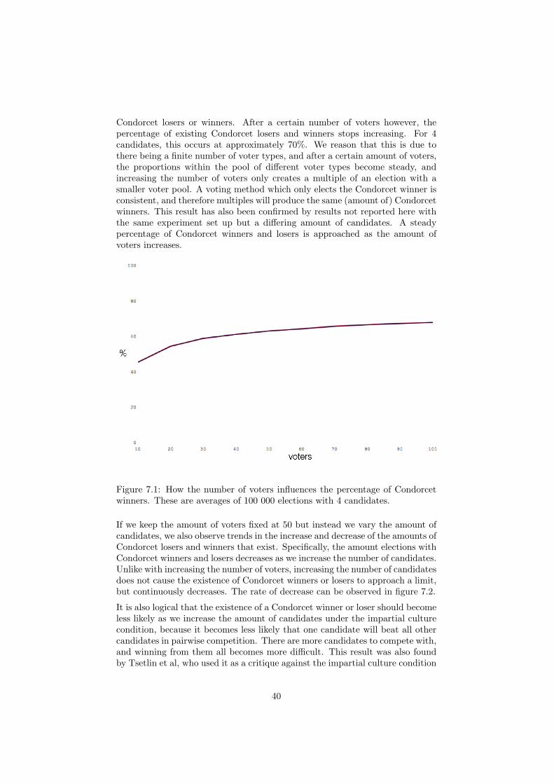
Condorcet losers or winners. After a certain number of voters however, thepercentage of existing Condorcet losers and winners stops increasing. For 4candidates, this occurs at approximately 70%. We reason that this is due tothere being a finite number of voter types, and after a certain amount of voters,the proportions within the pool of different voter types become steady, andincreasing the number of voters only creates a multiple of an election with asmaller voter pool. A voting method which only elects the Condorcet winner isconsistent, and therefore multiples will produce the same (amount of) Condorcetwinners. This result has also been confirmed by results not reported here withthe same experiment set up but a differing amount of candidates. A steadypercentage of Condorcet winners and losers is approached as the amount ofvoters increases.

Figure 7.1: How the number of voters influences the percentage of Condorcetwinners. These are averages of 100 000 elections with 4 candidates.

If we keep the amount of voters fixed at 50 but instead we vary the amount ofcandidates, we also observe trends in the increase and decrease of the amounts ofCondorcet losers and winners that exist. Specifically, the amount elections withCondorcet winners and losers decreases as we increase the number of candidates.Unlike with increasing the number of voters, increasing the number of candidatesdoes not cause the existence of Condorcet winners or losers to approach a limit,but continuously decreases. The rate of decrease can be observed in figure 7.2.

It is also logical that the existence of a Condorcet winner or loser should becomeless likely as we increase the amount of candidates under the impartial culturecondition, because it becomes less likely that one candidate will beat all othercandidates in pairwise competition. There are more candidates to compete with,and winning from them all becomes more difficult. This result was also foundby Tsetlin et al, who used it as a critique against the impartial culture condition

40

Figure 7.2: How the number of candidates influences the percentage of Con-dorcet winners. These are averages of 100 000 elections with 50 voters.

for voter generation [26].

41

7.2 Probability of Not Electing a Cordorcet Win-ner

The next experiment we ran involved the inspection of rules which do not satisfythe Condorcet criterion. Even though there are cases in which they will not electthe Condorcet winner, this only happens some of the time. Here we inspectexactly how often rules do not elect the Condorcet winner given the Condorcetwinner exists.

In figure 7.3 we can observe the increase in percentage of not electing the Con-dorcet winner. This graph has been generated from table 7.1, which shows theamount of times a Condorcet winner does get elected.

Figure 7.3: How often each rule does not elect the Condorcet winner. Averageof 100 000 elections.

We already know that Copeland will always elect the Condorcet winner whenone exists, and this is reflected in the graph. That approval and even and equalvery often do not elect the Condorcet winner is not that surprising, as theydo not take the ranking information which is crucial to the determination ofthe Condorcet winner into account. Similarly, although plurality does look atthe best ranked candidate, it ignores all other ballot information and thereforepredictably does very poorly as well.

The overall increase in the non-election of Condorcet winners can be explainedby the increased amount of candidates that a voting system might elect. Asthere are more candidates, any candidate a priori already has less chances ofbeing elected. If we were to assume a random voting method, which picks anycandidate from the candidates as a winner, we would also observe an increasein the amount of times a Condorcet winner is not elected. Voting methods suchas Copeland are specifically designed to deal with this trend, however, rules likeplurality are not.

42

no. cands 2 σ 3 σ 4 σ 5 σPlurality 100.0 0.0 79.19 4.79 68.09 5.69 59.55 6.46Borda 100.0 0.0 94.02 2.93 91.69 3.31 90.72 3.89Approval 100.0 0.0 76.32 4.95 67.64 5.78 62.06 6.70Even 100.0 0.0 74.57 4.90 66.31 5.72 59.23 6.56STV 100.0 0.0 96.80 2.04 93.73 2.97 90.62 3.98no. cands 6 σ 7 σ 8 σ 9 σPlurality 53.16 7.10 48.09 7.60 43.45 7.65 39.95 7.92Borda 90.20 4.21 89.69 4.54 89.944 4.49 90.26 5.16Approval 58.04 6.91 55.52 7.69 53.20 8.00 51.73 8.04Even 54.62 6.95 50.67 7.82 47.03 8.06 44.78 8.18STV 88.23 4.54 85.97 5.40 83.56 5.66 82.05 6.13

Table 7.1: How often do Condorcet winners get elected? In percent, average of100 000 elections with 50 voters.

Similar results have been obtained by Samuel Merrill III [19]. Under the impar-tial culture condition he ran 10 000 elections with 201 voters and 5 candidates,and determined that under these circumstances plurality would have a Con-dorcet efficiency of 60%, STV one of 88% and Borda one of 85% [19]. Here wefound 59.55%, 90.62% and 90.72% respectively. He also determined the Con-dorcet efficiency of approval voting to be 67%, but this is done with a votergeneration which differs from ours, which might explain the discrepancy fromour 62%.

43

7.3 Probability of Electing a Condorcet Loser

Another interesting criterion to analyse is the Condorcet loser criterion. Recallthat the Condorcet loser criterion requires the candidate who loses in pairwisecomparison to all other candidates must never be elected. Given that a ruledoes not satisfy the Condorcet loser criterion, how often is it the case that theCondorcet loser is elected by a given rule? Again we ran 100 000 elections witha varying amount of candidates to determine how well the different rules do.We collected the percentages of times that the rules would elect the Condorcetwinner when one existed. The results can be observed in figure 7.4, a graphgenerated from the data in table 7.2.

Figure 7.4: How often each rule elects the Condorcet Loser. Average of 100 000elections.

There is a very pronounced peak for most voting procedures at 3 candidates. Fortwo candidates it will never be the case for any voting rule that the Condorcetloser is elected, because all voting rules are then equal to plurality. Thereforeit is unsurprising there is a large difference between 2 and 3 candidates. Afterthe first 3 candidates, the amount of Condorcet losers elected decreases for allprocedures. Again, there is a larger a priori chance that any candidate wouldbe elected if there are less candidates, which explains why there is a decrease inthe election of Condorcet losers.

It has already been proven that Borda count will never elect the Condorcetloser [22], and this is reflected in our graph. Approval voting decreases fasterthan plurality and even and equal, which can be explained by the fact thatsecond, third, etc. ranked candidates still receive a large amount of points whenthey are approved in comparison to even and equal and plurality, which not onlypromotes them, but also helps in distinguishing from the last ranked candidates.

44

no. cands 2 σ 3 σ 4 σ 5 σPlurality 0.00 0.00 1.40 1.39 1.10 1.31 0.82 1.21Borda 0.00 0.00 0.00 0.00 0.00 0.00 0.00 0.00Approval 0.00 0.00 1.53 1.42 0.72 1.06 0.34 0.80Even 0.00 0.00 2.80 1.92 2.03 1.75 1.38 1.58STV 0.00 0.00 0.32 0.68 0.19 0.56 0.11 0.43no. cands 6 σ 7 σ 8 σ 9 σPlurality 0.67 1.11 0.53 1.12 0.49 1.11 0.37 1.03Borda 0.00 0.00 0.00 0.00 0.00 0.00 0.00 0.00Approval 0.21 0.63 0.12 0.50 0.05 0.36 0.02 0.21Even 1.09 1.47 0.76 1.31 0.63 1.26 0.54 1.21STV 0.07 0.38 0.04 0.31 0.011 0.17 0.01 0.17

Table 7.2: How often are Condorcet losers elected? In percent, average of 100000 elections and 50 voters.

7.4 How often do voting rules elect the samecandidates?

For groups of randomly generated candidates and voters adhering to the im-partial culture condition, we calculated the percentage of times that the votingrules would agree with each other. In all cases, we generated 10000 electionswith 50 voters, with respectively 3, 4 and 5 candidates. With 2 candidates thevoting rules all agree 100% of the time because then they all mirror plurality,but as the number of candidates increases this number diverges.

Plurality Borda Approval Even STV CopelandPlurality 100.0 70.5 59.6 63.72 70.96 66.23Borda 70.5 100.0 69.34 67.4 75.66 81.32Approval 59.6 69.34 100.0 79.85 62.65 64.0Even 63.72 67.4 79.85 100.0 62.56 62.52STV 70.96 75.66 62.65 62.56 100.0 85.62Copeland 66.23 81.32 64.0 62.52 85.62 100.0

Table 7.3: Average of 10000 elections with 3 candidates and 50 voters



45



7.5 From Plurality to Borda to Antiplurality

Recall that a positional scoring vector assigns points to candidates dependingon where they are in the ranking. Plurality: 〈1, 0, 0〉, Borda count: 〈1, 1

2 , 0〉,antiplurality: 〈1, 1, 0〉.For 3 candidates this could be generalized as: 〈1, λ, 0〉 for λ ∈ [0, 1], where allthe scoring vectors we create by varying λ represent different voting procedures.We know that Borda count does not elect the Condorcet loser [22], and we knowthat plurality does. When does this change? When we examine these unnamedvoting rules, how often do they elect the Condorcet winner and loser?

λ Condorcet winners not elected σ0.0 20.7569710672 4.693829935210.1 13.1364955705 3.889693204570.2 10.2866459258 3.501703502420.3 6.7884043218 2.904419926680.4 4.9678354044 2.507726747550.5 5.8773270604 2.730393702710.6 6.2252217648 2.827819655710.7 9.0160946185 3.325803274780.8 13.7318585388 3.991384764350.9 17.5088685503 4.435005790431.0 26.0178407320 5.11604112681

Table 7.6: Average of 1 000 000 elections with 3 candidates and 50 voters.

In both tables we can see that Borda count does the best in electing Condorcetwinners and not electing Condorcet losers, and the results monotonically worsenas we increase or decrease the λ from 0.5. These results more or less match theresults found by Gehrlein in his 1996 paper, where he ran the same experimentbut does not mention with how many voters or how many elections he averaged[12]. He also varies λ from 0 to 0.5, and we vary λ from 0 to 1 in step sizes of0.1.

46

λ Condorcet losers elected σ0.0 1.4145844893 1.368434300730.1 1.2165588940 1.268358256730.2 0.5421445603 0.845997604210.3 0.0681647892 0.298908637420.4 0.0008184719 0.033445562220.5 0.0000000000 0.000000000000.6 0.0009523477 0.035999498490.7 0.0938891876 0.354788747610.8 0.5935236318 0.881037906510.9 1.3747336139 1.335094563721.0 1.7763837257 1.52177847947


7.6 From classic approval to even and equal

Recall size approval voting, where the amount of points is dependent on theamount of approved candidates. All size approval voting rules can be definedby a weight vector. If k candidates are approved, they all receive the amount ofpoints specified in the kth position of the weight vector. For classic approval theweight vector is homogenous: 〈1, 1, 1〉, and for even and equal it decreases as 1

kdecreases. For three candidates, the weight vector for even and equal becomes〈1, 1

2 , 13 〉.

For 3 candidates, the weight vector could be generalized as: 〈1, λ〉 for λ ∈ [0, 1].Since at most n − 1 candidates can be approved, n being the total number ofcandidates, the weight vector also only needs to be n− 1 long.

There are now many unnamed voting rules between classic approval and evenand equal size approval voting for 3 candidates. When we examine these un-named voting rules, how often do they elect the Condorcet winner and loser?

λ Condorcet winners not elected σ0.0 41.4607972575 5.665616837190.1 32.4272765144 5.397818298750.2 29.8731661125 5.296642731810.3 26.9514371539 5.123692317050.4 24.8074485792 4.949411383710.5 25.0430820551 4.972247951270.6 21.6506186499 4.736602521820.7 20.5394122957 4.637645015620.8 20.0271627413 4.587105238930.9 19.6000146242 4.551792318531.0 23.2970908415 4.86697819586


λ = 0.0 is of course a bit of an odd case: if more than 1 candidate is approved, nopoints are assigned. This translates to half of the voters really abstaining from

47

the election, for their votes have no effect. The other half of the voters votingaccording to the plurality rule. Both λ = 1 and λ = 0.5 agree with previousresults we obtained when running experiments with named procedures, butλ = 0 is incomparable to the effects of half the voters abstaining.

λ Condorcet losers elected σ0.0 7.80094044005 3.085114529670.1 8.13535203584 3.161738587300.2 6.50226128269 2.861366495030.3 5.10938882109 2.541749033360.4 3.85881210210 2.235627673990.5 2.76132073023 1.889624619900.6 2.75264332602 1.885075809780.7 2.45252118512 1.787786279750.8 2.25656247742 1.715621949770.9 2.26258875927 1.721615123721.0 1.57445306300 1.43468100974


In the previous experiments we named procedures we also noticed that evenand equal performs more poorly than approval voting in electing the Condorcetloser. With this experiment we observe that this is a trend that increases as wedecrease λ. As λ decreases, the amount of Condorcet losers elected increases.We still think this is due 2nd and 3rd ranked candidates receiving less points,and therefore not distinguishing themselves significantly from the last rankedcandidates.

48

Chapter 8

Discussion

Some of the experiments we ran brought up certain issues and results that wefound surprising or interesting enough to bring up separately.

8.1 Approving of all candidates

In our implementation, we do not generate voters with a cut-off point whichis before the first or after the last candidate. Approving of all candidates orapproving of no candidates does not change the outcome of the approval oreven and equal election. However, when comparing the outcomes of differentelection systems, approving of all candidates can cause the outcome to differ.

Our smallest election for which Borda count and approval voting differ is asfollows:


1 voter: C2 | C1 > C0

However, one might notice that the same outcome could be achieved if weremoved candidate C0 entirely, and thus would provide us with an electioninstance with only two candidates.

2 voters: C1 > C2 |1 voter: C2 | C1

If we were to allow approval of all candidates, or really abstention in our searchfor the smallest elections, we might find even smaller election instances. How-ever, it is a theoretical situation which does not occur practically. For thisreason, we find our original results more interesting.

49

8.2 Selection of candidate to eliminate in Hare’smethod

One of the things which was surprising in the Condorcet loser election exper-iments (see section 7.3) is that STV also elects the Condorcet loser at times,while STV is commonly assumed to satisfy the Condorcet loser criterion. Afterinspection of the elections where this was the case, we found that it was due toour implementation of STV: if there is a tied last place in plurality, we removeboth last placed candidates simultaneously. However, when doing this we mightalso cause the Condorcet loser to be elected.

Imagine the following election between candidates A, B and C:

2 voters: A > B > C2 voters: B > A > C3 voters: C > A > B

Because A and B are both the least first ranked of the candidates, we removethem both. However, the only candidate who then remains is C, who is actuallythe Condorcet loser.

Coombs’ method avoids this problem by selecting the antiplurality loser, anddoes satisfy the Condorcet loser criterion.

Hare has not formally determined what to do in case of a tie for pluralityloser, and neither have other sources on how STV is used. This might beconsidered odd, because STV is used for many governmental elections, but thecase described above would only happen for very small amounts of voters andtherefore would hardly ever arise in real life.

50

Chapter 9

Conclusion and FutureWork

We have examined many different voting procedures. First we examined theirdefinitions and characteristics they are theoretically known to possess. Then weexamined how we can make the smallest election instances where different votingprocedures elect different candidates. To be able to do this, we implemented acomparative framework which can take the same ballots and run elections withmany different voting procedures.

Using our comparative framework, we also ran statistical experiments whichwould give an indication of how often certain rules fail certain criteria if they arealready theoretically known to at times do so. We checked how often differentnon-Condorcet criterion satisfying voting procedures would not elect the Con-dorcet winner when one exists. Similarly, we checked how often non-Condorcetloser criterion satisfying rules would actually elect the Condorcet loser. Wefound that this happens very infrequently, even for notoriously deviant rulessuch as approval voting.

We examined unnamed positional scoring voting procedures for 3 candidateelections, and found that as we deviate from Borda count towards pluralityor antiplurality, the amount of times the Condorcet winner is not elected orthe Condorcet loser is elected increases monotonically. We examined unnamedapproval voting procedures for 3 candidate elections as well, and found that forsize approval voting, assigning multiple approved candidates less points thansingle approved candidates causes it to be more likely that the Condorcet loseris elected as the amount of points decreases.

We compared how often different voting procedures would elect the same win-ners, and found that as we increase the number of participating candidates allvoting rules diverge more in electing different candidates. This divergence isvery sharp at the beginning, with very large drops from 2 to 3 candidates andfrom 3 to 4, but this the decrease slows and may approach some limit. It wouldbe interesting to continue work with this experiment to determine exactly whatthis limit is.

51

For the smallest election instances, we increased the amount of voters beforeincreasing the amount of candidates participating. It is possible that we couldhave found an example with 4 candidates and 2 voters where our examples have3 candidates and 3 voters. It would be interesting to continue finding theseinstances and comparing them to each other.

We were unable to find the smallest election instance where Copeland wouldelect a different candidate than Dodgson. To be able to do this and also runother larger elections with Dodgson, we would like to implement the heuristicproposed for finding the Dodgson winner in the future.

Many of the results we found had 3 or more variables to display, we would beinterested in finding a better way to display the data and perhaps be able tomanipulate which parameters are being shown in real time, to make the datamore easy to understand.

Finally, we would like to implement more voting procedures in our comparativeframework as well as different ways of automatic voter generation, to be able torun experiments with these as well.

52

Acknowledgements

This work was done as my bachelor’s thesis in AI at the University of Amster-dam. It was done in the context of the AI honours programme.

I would like to thank Ulle Endriss for being absolutely the best possible teacherand thesis advisor− from introducing me to the topic to poring over buggyresults. I would also like to thank him for coordinating the honours programmeand supervising my first research project, which is really the main reason I leftart school for AI.

I would also like to thank Marco Wessel for the constant influx of consumptableswithout which I would have long since withered away, and allowing me to usehis servers for experiment running and repository hosting. I think he might usethe word awesometastic.

Finally I would like to thank fellow honours students Gijs Kruitbosch and HylkeBuisman for giving random advice at random hours, and also all my classmatesfor all their help and coffee donations.

The poem at the beginning is taken entirely without permission from DamienHirst’s latest book Superstition.

53

Bibliography

[1] Jorge Alcalde-Unzu and Marc Vorsatz, Size approval voting, ResearchMemorandum 008, Maastricht : METEOR, Maastricht Research Schoolof Economics of Technology and Organization, 2007.

[2] John H. Aldrich, Before the convention, University of Chicago Press,Chicago, 1980.

[3] Kenneth Arrow, A difficulty in the concept of social welfare, Journal ofPolitical Economy 58 (1950), no. 4, 328–346.

[4] Duncan Black, The theory of committees and elections, Cambridge Univer-sity Press, 1958.

[5] Steven J. Brams and Peter C. Fishburn, Approval voting, The AmericanPolitical Science Review 72 (1978), no. 3, 831–847.

[6] US Federal Election Commission, 2000 presidential electoral and popularvote, 2000, http://www.fec.gov/pubrec/fe2000/elecpop.htm.

[7] Conseil Constitutionnel, Election presidentielle 2002, 2002, http://www.conseil-constitutionnel.fr/dossier/presidentielles/2002.

[8] Arthur H. Copeland, A ‘reasonable’ social welfare function, Seminar onmathematics in social sciences, University of Michigan, 1951.

[9] O. Davis, M. Hinich, and P. Ordeshook, An expository development ofa mathematical model of the electoral process, American Political ScienceReview 68 (1970), 426–448.

[10] Jean Charles de Borda, Memoire sur les elections au scrutin, Histoire del’Academie Royale des Sciences, 1781.

[11] Anthony Downs, An economic theory of democracy, Harper and Row, NewYork, 1957.

[12] William V. Gehrlein, The probability of electing the condorcet loser, Pro-ceedings of National Decision Sciences Institute 2 (1996), no. 111.

[13] Alan Gibbard, Manipulation of voting schemes: a general result, Econo-metrica 41 (1973), no. 4, 587–601.

54

http://www.fec.gov/pubrec/fe2000/elecpop.htm

http://www.conseil-constitutionnel.fr/dossier/presidentielles/2002

http://www.conseil-constitutionnel.fr/dossier/presidentielles/2002

[14] Bernard Grofman and Scott L. Feld, If you like the alternative vote (a.k.a.the instant runoff), then you ought to know about the Coombs rule, Elec-toral Studies 23 (2004), no. 4, 641–659.

[15] Thomas Hare, The machinery of representation, 1857.

[16] Peter E. Hart, Nils J. Nilsson, and Bertram Raphael, A formal basis forthe heuristic determination of minimum cost paths, IEEE Transactions onSystems Science and Cybernetics 4 (1968), no. 2, 100–107.

[17] Edith Hemaspaandra, Lane A. Hemaspaandra, and Jorg Rothe, Exact anal-ysis of Dodgson elections: Lewis Carroll’s 1876 voting system is completefor parallel access to NP, J. ACM 44 (1997), no. 6, 806–825.

[18] John J. Bartholdi III, Craig A. Tovey, and Michael A. Trick, Voting schemesfor which it can be difficult to tell who won the election, Social Choice andWelfare 6 (1989), no. 2, 157–165.

[19] Samuel Merrill III, A comparison of efficiency of multicandidate electoralsystems, American Journal of Political Science 28 (1984), no. 1, 23–48.

[20] Philip D. Straffin Jr., Topics in the theory of voting, Birkhauser, Boston,1980.

[21] John C. McCabe-Dansted, Geoffrey Pritchard, and Arkadii Slinko, Ap-proximability of Dodgsons rule, Social Choice and Welfare 31 (2008), no. 2,311–330.

[22] Hannu Nurmi, Comparing voting systems, D. Reidel Publishing, Dordrecht,the Netherlands, 1987.

[23] Michel Regenwetter and Ilia Tsetlin, Approval voting and positional votingmethods: Inference, relationship, examples, Social Choice and Welfare 22(2004), no. 3, 539–566.

[24] Mark A. Satterthwaite, Strategy-proofness and Arrow’s conditions: Exis-tence and correspondence theorems for voting procedures and social welfarefunctions, Journal of Economic Theory 10 (1975), no. 1, 187–217.

[25] T. N. Tideman, Independence of clones as a criterion for voting rules,Social Choice and Welfare 4 (1987), no. 3, 185–206.

[26] Ilia Tsetlin, Michel Regenwetter, and Bernard Grofman, The impartial cul-ture maximizes the probability of majority cycles, Social Choice and Welfare21 (2003), no. 3, 387–398.

55

Documents

Automatic Analysis of Voting Procedures · For this thesis we compared a selection of voting procedures in two ways. Firstly ... One could also consider that the voting system the