Embed Size (px)
Citation preview

University of Kentucky University of Kentucky
UKnowledge UKnowledge
Theses and Dissertations--Computer Science Computer Science
2018
AUTOMATED TREE-LEVEL FOREST QUANTIFICATION USING AUTOMATED TREE-LEVEL FOREST QUANTIFICATION USING
AIRBORNE LIDAR AIRBORNE LIDAR
Hamid Hamraz University of Kentucky, [email protected] Digital Object Identifier: https://doi.org/10.13023/etd.2018.239
Right click to open a feedback form in a new tab to let us know how this document benefits you. Right click to open a feedback form in a new tab to let us know how this document benefits you.
Recommended Citation Recommended Citation Hamraz, Hamid, "AUTOMATED TREE-LEVEL FOREST QUANTIFICATION USING AIRBORNE LIDAR" (2018). Theses and Dissertations--Computer Science. 69. https://uknowledge.uky.edu/cs_etds/69
This Doctoral Dissertation is brought to you for free and open access by the Computer Science at UKnowledge. It has been accepted for inclusion in Theses and Dissertations--Computer Science by an authorized administrator of UKnowledge. For more information, please contact [email protected].

STUDENT AGREEMENT: STUDENT AGREEMENT:
I represent that my thesis or dissertation and abstract are my original work. Proper attribution
has been given to all outside sources. I understand that I am solely responsible for obtaining
any needed copyright permissions. I have obtained needed written permission statement(s)
from the owner(s) of each third-party copyrighted matter to be included in my work, allowing
electronic distribution (if such use is not permitted by the fair use doctrine) which will be
submitted to UKnowledge as Additional File.
I hereby grant to The University of Kentucky and its agents the irrevocable, non-exclusive, and
royalty-free license to archive and make accessible my work in whole or in part in all forms of
media, now or hereafter known. I agree that the document mentioned above may be made
available immediately for worldwide access unless an embargo applies.
I retain all other ownership rights to the copyright of my work. I also retain the right to use in
future works (such as articles or books) all or part of my work. I understand that I am free to
register the copyright to my work.
REVIEW, APPROVAL AND ACCEPTANCE REVIEW, APPROVAL AND ACCEPTANCE
The document mentioned above has been reviewed and accepted by the student’s advisor, on
behalf of the advisory committee, and by the Director of Graduate Studies (DGS), on behalf of
the program; we verify that this is the final, approved version of the student’s thesis including all
changes required by the advisory committee. The undersigned agree to abide by the statements
above.
Hamid Hamraz, Student
Dr. Nathan Jacobs, Major Professor
Dr. Miroslaw Truszczynski, Director of Graduate Studies

AUTOMATED TREE-LEVEL FOREST QUANTIFICATION USING AIRBORNE LIDAR
DISSERTATION
A dissertation submitted in partial fulfillment of the requirement for the degree of Doctor of Philosophy in the College of Engineering at the University of Kentucky
By Hamid Hamraz
Lexington, Kentucky
Directors Dr. Nathan Jacobs, Professor of computer science And Dr. Marco Contreras, Professor of Forestry and Natural Resources
Lexington, Kentucky 2018
Copyright © Hamid Hamraz 2018

ABSTRACT OF DISSERTATION
AUTOMATED TREE-LEVEL FOREST QUANTIFICATION
USING AIRBORNE LIDAR
Traditional forest management relies on a small field sample and interpretation of aerial photography that not only are costly to execute but also yield inaccurate estimates of the entire forest in question. Airborne light detection and ranging (LiDAR) is a remote sensing technology that records point clouds representing the 3D structure of a forest canopy and the terrain underneath. We present a method for segmenting individual trees from the LiDAR point clouds without making prior assumptions about tree crown shapes and sizes. We then present a method that vertically stratifies the point cloud to an overstory and multiple understory tree canopy layers. Using the stratification method, we modeled the occlusion of higher canopy layers with respect to point density. We also present a distributed computing approach that enables processing the massive data of an arbitrarily large forest. Lastly, we investigated using deep learning for coniferous/deciduous classification of point cloud segments representing individual tree crowns. We applied the developed methods to the University of Kentucky Robinson Forest, a natural, majorly deciduous, closed-canopy forest. 90% of overstory and 47% of understory trees were detected with false positive rates of 14% and 2% respectively. Vertical stratification improved the detection rate of understory trees to 67% at the cost of increasing their false positive rate to 12%. According to our occlusion model, a point density of about 170 pt/m² is needed to segment understory trees located in the third layer as accurately as overstory trees. Using our distributed processing method, we segmented about two million trees within a 7400-ha forest in 2.5 hours using 192 processing cores, showing a speedup of ~170. Our deep learning experiments showed high classification accuracies (~82% coniferous and ~90% deciduous) without the need to manually assemble the features. In conclusion, the methods developed are steps forward to remote, accurate quantification of large natural forests at the individual tree level. Keywords: remote sensing, point cloud processing, horizontal/vertical segmentation, occlusion modeling, distributed computing, deep learning.
Hamid Hamraz April 9, 2018

AUTOMATED TREE-LEVEL FOREST QUANTIFICATION USING AIRBORNE LIDAR
By Hamid Hamraz
Nathan Jacobs Co-Director of Dissertation
Marco Contreras Co-Director of Dissertation
Miroslaw Truszczynski Director of Graduate Studies
April 9th, 2018 Date

iii
Acknowledgements
I would hereby like to express my gratitude to my advisors, Dr. Jacobs and Dr. Contreras,
for their helps, supports, advices, and the lessons taught to me throughout my Ph.D.
endeavor. I would also like to thank my Ph.D. committee members specially Dr.
Manivannan for their supports of my work. Moreover, I would also like to give
recognition to the advices and pointers offered by my previous advisor, Dr. Zhang, that
helped me identify the current dissertation project and to his support that helped me
establish and pursue my Ph.D. research. Special thanks goes to Dr. Goldsmith for her
initial support that enabled me start the Computer Science Ph.D. program at the
University of Kentucky. I would also like to appreciate the supports of Dr. Marek and Dr.
Calvert before I identified a research advisor and landed my Ph.D. research project. Dr.
Calvert has specially offered financial support for my research work multiple times
during the summers so as I could keep focused on my research work.
My wife, Mojdeh Nakhaei, has provided not only emotional support but also technical
help such as graphical designs several times throughout my Ph.D. endeavor and I would
like to express my sincere gratitude to her as well. Last but not least, I would also like to
show my appreciation to my parents for their unparalleled efforts throughout my life and
for their support of my education and academic growth both in my home country and in
the United States.
Funding-wise, my Ph.D. research project was supported by: i) the Department of Forestry
at the University of Kentucky and the McIntire-Stennis project KY009026 Accession
1001477, ii) the Kentucky Science and Engineering Foundation under the grant number
KSEF-3405-RDE-018, iii) the University of Kentucky Center for Computational
Sciences, iv) the Gartner Group Professorship in Network Engineering at the University
of Kentucky, and v) the National Science Foundation under Grant Number CCF-
1215985. I hereby would like to appreciate these agencies for their support that made this
work possible.

iv
Table of Contents Acknowledgements ......................................................................................................................... iii
Table of Contents ............................................................................................................................ iv
List of Tables ................................................................................................................................. vii
List of Figures ............................................................................................................................... viii
1 Introduction and Basics ............................................................................................................ 1
1.1 Forest management .............................................................................................. 1
1.2 LiDAR technology ............................................................................................... 1
1.3 Airborne LiDAR for forest management ............................................................. 2
1.4 Motivation and current dissertation...................................................................... 3
2 Individual Tree Segmentation .................................................................................................. 6
2.1 Literature review .................................................................................................. 6
2.2 Research materials................................................................................................ 8
2.2.1 Study site .................................................................................................................. 8
2.2.2 Recent field survey ................................................................................................ 10
2.2.3 LiDAR dataset ....................................................................................................... 11
2.3 Tree segmentation method ................................................................................. 12
2.3.1 Profile generation ................................................................................................... 16
2.3.2 Crown boundary identification .............................................................................. 17
2.3.2.1 Identification of inter-crown gaps ...................................................................... 17
2.3.2.2 Identifying local minima points as crown boundaries ....................................... 19
2.4 Evaluation........................................................................................................... 21
2.4.1 Ground truth field data ........................................................................................... 21
2.4.2 Evaluation procedure ............................................................................................. 23
2.5 Results and discussion ........................................................................................ 25
2.5.1 Segmentation accuracy .......................................................................................... 25
2.5.2 Applicability to different conditions ...................................................................... 28
2.6 Conclusion .......................................................................................................... 29
2.A. Expected slope of a spherical surface ................................................................ 31
3 Vertical Stratification ............................................................................................................. 32

v
3.1 Literature review ................................................................................................ 33
3.2 Methods .............................................................................................................. 34
3.2.1 Vertical stratification of canopy ............................................................................. 34
3.2.2 Canopy occlusion model ........................................................................................ 38
3.3 Results ................................................................................................................ 39
3.3.1 Segmentation accuracy .......................................................................................... 39
3.3.2 Stratified canopy layers .......................................................................................... 43
3.3.3 Canopy occlusion ................................................................................................... 45
3.4 Discussion .......................................................................................................... 47
3.5 Conclusion .......................................................................................................... 49
4 Processing Large-Scale LiDAR Data .................................................................................... 51
4.1 Literature review ................................................................................................ 51
4.2 Distributed computing ........................................................................................ 53
4.2.1 Big LiDAR data of Robinson Forest ...................................................................... 53
4.2.2 Distributed tree segmentation ................................................................................ 54
4.2.3 Theoretical runtime analysis .................................................................................. 58
4.3 Results and discussions ...................................................................................... 60
4.3.1 Runtime and scalability .......................................................................................... 60
4.3.2 Implementation and using Hadoop MapReduce .................................................... 63
4.3.3 Generalization to other spatial datasets .................................................................. 64
4.3.4 Global parameters of Robinson Forest ................................................................... 65
4.4 Conclusion .......................................................................................................... 70
4.A Implementation of segmentation algorithm and runtime analysis ..................... 72
5 Deep Learning for Predicting Tree Type ............................................................................... 75
5.1 Literature review ................................................................................................ 76
5.2 Data preparation ................................................................................................. 77
5.2.1 Intensity normalization .......................................................................................... 78
5.2.2 Registration with field data .................................................................................... 78
5.2.3 Discretization of crown point clouds and data augmentation ................................ 79

vi
5.3 Deep learning ..................................................................................................... 80
5.3.1 Convolutional neural network models ................................................................... 80
5.3.2 Mislabel correction via iterative resampling .......................................................... 81
5.3.3 Classification and evaluation ................................................................................. 83
5.4 Results and discussions ...................................................................................... 84
5.4.1 Mislabel correction ................................................................................................ 84
5.4.2 Classification accuracy .......................................................................................... 86
5.4.3 Effect of training data size ..................................................................................... 87
5.4.4 Effect of data augmentation ................................................................................... 88
5.4.5 Effect of domain data ............................................................................................. 89
5.4.6 Effects of crown class and point density ................................................................ 92
5.5 Conclusions ........................................................................................................ 93
6 Conclusions and Future Directions ........................................................................................ 95
6.1 Summary of technical contributions .................................................................. 95
6.2 Summary of results............................................................................................. 97
6.3 Potential improvements and future directions .................................................... 99
6.4 Implications for forest management and beyond ............................................. 102
References .................................................................................................................................... 105
Vita ............................................................................................................................................. 122

vii
List of Tables
Table 2.1. Summary of plot level data collected from the 271 plots in Robinson Forest. 11
Table 2.2. LiDAR data acquisition parameters used for both datasets collected over
Robinson Forest. ............................................................................................................... 12
Table 2.3. Summary of plot level data collected from the 23 accurately georeferenced
plots in Robinson Forest. .................................................................................................. 22
Table 2.4. Leaning and height difference thresholds with associated scores considered for
matching LiDAR-derived tree locations to stem map locations. ...................................... 23
Table 2.5. Summary of accuracy results of the tree segmentation approach on the 23
plots. .................................................................................................................................. 26
Table 3.1. Summary of two-tailed paired T-tests assessing the improvement of canopy
stratification for tree segmentation. .................................................................................. 42
Table 3.2. Summary statistics of canopy layers over the 50,911 sample plots regularly
distributed in Robinson Forest. ......................................................................................... 44
Table 4.1. Estimated number of trees categorized based on tree crown class. ................. 67
Table 5.1. Summary statistics of trees surveyed within 271 plots in Robinson Forest
categorized based on tree type. ......................................................................................... 77

viii
List of Figures
Figure 2.1. Terrain relief map of the University of Kentucky Robinson Forest and its
general location within Kentucky, USA. ............................................................................ 9
Figure 2.2. Aerial image of the camp and a glimpse over the canopy at Robinson Forest
in Clayhole, KY ccaptured in August 2016 (credit: Matt Barton, Agricultural
Communications Services – University of Kentucky). ..................................................... 10
Figure 2.3. Flowchart of the tree segmentation method used to identify tree locations and
segment tree crowns. ......................................................................................................... 14
Figure 2.4. Illustration of the preprocessing steps and the five routines within the tree
segmentation approach...................................................................................................... 15
Figure 2.5. Diagram illustrating the calculation of the chord height (x) formed by two
profiles of maximum crown radius (r) separated by the angular spacing (φ). .................. 16
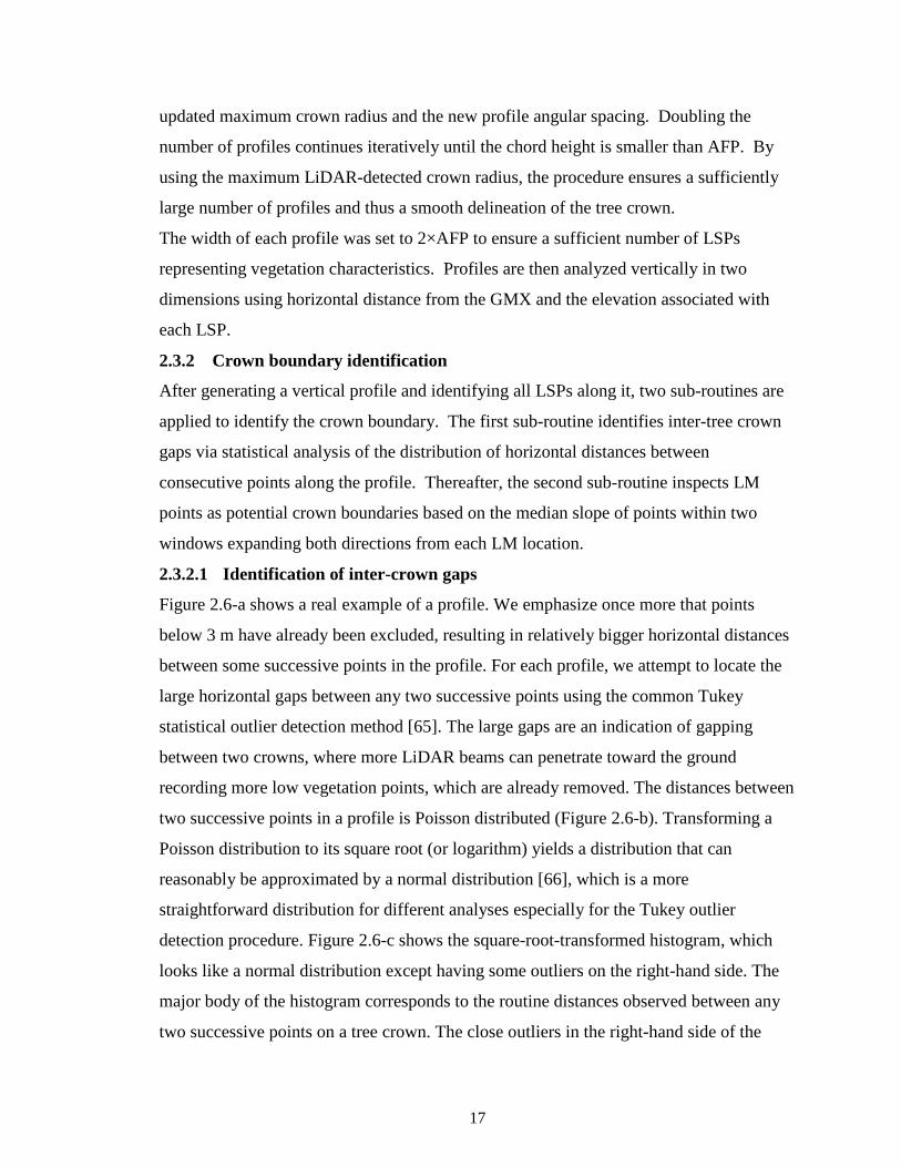
Figure 2.6. a) A real example of a profile (a potential inter-crown gap is highlighted); b)
Poisson distribution of the distances between any two successive point in the profile; c)
square root Transformed distribution of the distances looking like a normal distribution
for the major part (the outlier corresponding to the inter-crown gap is highlighted); d)
trimming the profile from the gaps on both sides of the GMX. ....................................... 18
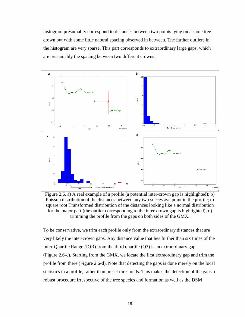
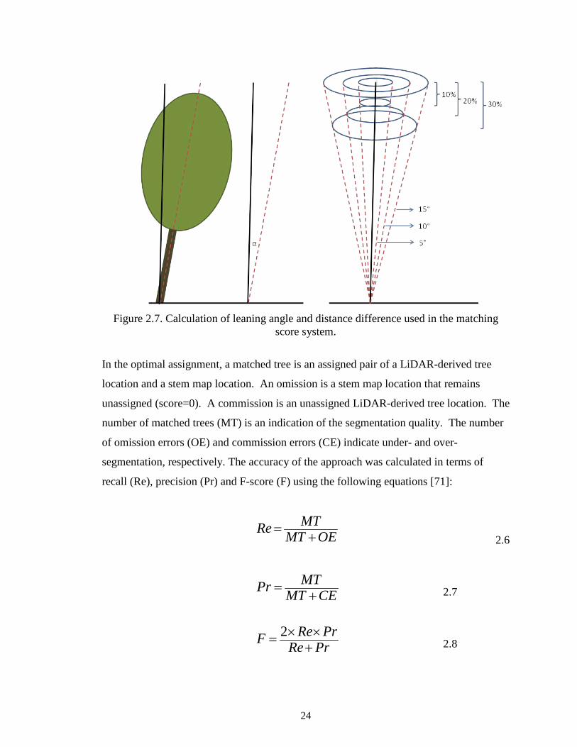
Figure 2.7. Calculation of leaning angle and distance difference used in the matching
score system. ..................................................................................................................... 24
Figure 2.8. Aerial visualization of the tree segmentation results in four plots within the
study area. Distinct colors represent matched tree crowns. .............................................. 28
Figure 2.9. The angle α representing the slope of the unit circle is a function of x. ......... 31
Figure 3.1. Height histogram of LiDAR points within a locale including over 100 points
used for determining the height threshold for removing the top canopy layer in a cell
location. ............................................................................................................................. 35
Figure 3.2. Illustration of the tree segmentation process in a multi-story stand by
stratifying one canopy layer at a time, removing it from the point cloud, and segmenting
crowns within each layer. ................................................................................................. 37
Figure 3.3. Average segmentation accuracies over the 271 sample plots grouped by
crown class. ....................................................................................................................... 41
Figure 3.4. Thickness of canopy layer according to starting height of the layer. ............. 44
ix
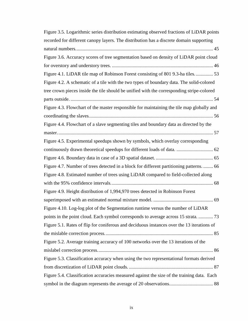
Figure 3.5. Logarithmic series distribution estimating observed fractions of LiDAR points
recorded for different canopy layers. The distribution has a discrete domain supporting
natural numbers. ................................................................................................................ 45
Figure 3.6. Accuracy scores of tree segmentation based on density of LiDAR point cloud
for overstory and understory trees. ................................................................................... 46
Figure 4.1. LiDAR tile map of Robinson Forest consisting of 801 9.3-ha tiles. .............. 53
Figure 4.2. A schematic of a tile with the two types of boundary data. The solid-colored
tree crown pieces inside the tile should be unified with the corresponding stripe-colored
parts outside. ..................................................................................................................... 54
Figure 4.3. Flowchart of the master responsible for maintaining the tile map globally and
coordinating the slaves. ..................................................................................................... 56
Figure 4.4. Flowchart of a slave segmenting tiles and boundary data as directed by the
master. ............................................................................................................................... 57
Figure 4.5. Experimental speedups shown by symbols, which overlay corresponding
continuously drawn theoretical speedups for different loads of data. .............................. 62
Figure 4.6. Boundary data in case of a 3D spatial dataset. ............................................... 65
Figure 4.7. Number of trees detected in a block for different partitioning patterns. ........ 66
Figure 4.8. Estimated number of trees using LiDAR compared to field-collected along
with the 95% confidence intervals. ................................................................................... 68
Figure 4.9. Height distribution of 1,994,970 trees detected in Robinson Forest
superimposed with an estimated normal mixture model. ................................................. 69
Figure 4.10. Log-log plot of the Segmentation runtime versus the number of LiDAR
points in the point cloud. Each symbol corresponds to average across 15 strata. ............ 73
Figure 5.1. Rates of flip for coniferous and deciduous instances over the 13 iterations of
the mislable correction process. ........................................................................................ 85
Figure 5.2. Average training accuracy of 100 networks over the 13 iterations of the
mislabel correction process. .............................................................................................. 86
Figure 5.3. Classification accuracy when using the two representational formats derived
from discretization of LiDAR point clouds. ..................................................................... 87
Figure 5.4. Classification accuracies measured against the size of the training data. Each
symbol in the diagram represents the average of 20 observations.................................... 88

x
Figure 5.5. Classification accuracies measured against the number of rotational
augmentations per instance. .............................................................................................. 89
Figure 5.6. Classification accuracies when excluding domain data. ................................ 91
Figure 5.7. Classification accuracy of overstory and understory trees. ............................ 93

1
1 Introduction and Basics
1.1 Forest management
Traditionally, decision making in forest management has been based on attributes of
stands, which are forested areas with similar vegetation characteristics. These attributes
are derived using a sample of field measurements and interpretation of aerial photography
[1-3]. Field measurements usually includes the number of trees, tree species, diameter at
breast height (DBH), tree height, and crown width that together with the aerial imagery
can provide estimates of global stand attributes. Because field-based inventory data are
expensive and labor-intensive to acquire, sampling of field measurements is limited and
adds up to a small fraction. This limited sampling results in rough estimates of stand
attributes and ignores large variability in terrain and vegetation structure within stands.
Recent advances in remote sensing, geographic information systems (GIS), and
information science technologies have the potential to bring dramatic changes to forest
data acquisition and management by providing inventory data at unprecedented spatial
and temporal resolutions [4-7]. For instance, high-resolution aerial images have been
processed to map forests and monitor their growth and regeneration [8-10]. However, 2D
images, as snapshots of the 3D world, lose depth information and are insufficient for
more detailed estimation tasks such as the derivation of vertical canopy structure and
biomass quantification. Airborne light detection and ranging (LiDAR) can record 3D
point clouds representing the forest canopy and the terrain underneath over large
geographical regions [11-14]. These LiDAR point clouds have been used to derive more
accurate stand attributes including tree locations, heights, and crown widths [15, 16].
1.2 LiDAR technology
LiDAR is an active remote sensing technology that emits pulses of energy that come into
contact with objects and then are reflected back toward the sensor. The time that elapses
when a pulse is emitted and its return to the LiDAR sensor is used to calculate the
distance, which is referred to as range. Given the global positioning system (GPS)
coordinates of the sensor and its orientation, the coordinates of the returning point can be
calculated. LiDAR pulses have the capability of penetrating beyond non-opaque surfaces
and thus can record multiple returns per a single emission. Depending on the surface

2
orientation, its reflective properties, as well as the atmospheric conditions, the intensity
values of the returns vary, which can also be recorded by the LiDAR sensors.
Airborne LiDAR sensors are designed for aerial surveys and emit multiple hundreds of
thousand pulses per second. Pulse emissions are linked with an on-board GPS receiver
and an inertial navigation unit to obtain the sensor coordinates and orientation with each
pulse in real time. The LiDAR sensors have an internal actuator mechanism that enables
oscillation of the emission orientation within an adjustable field of view. Given the
aircraft forward move and the LiDAR sensor facing toward the ground, an airborne
LiDAR system can scan a zigzag pattern, collecting 3D point clouds that represent the
objects and terrain over large areas [12, 17].
LiDAR 3D point clouds are commonly used to derive surface models [18] to represent
the elevation of objects (digital surface model, DSM) as well as the elevation of the bare
ground (digital elevation model, DEM). These surface models have a myriad of
applications in natural resources, flood modeling, mapping, urban planning, coastal
engineering, civil and transportation, etc. The surface models generated from airborne
LiDAR point clouds have successfully been used to identify features in urban landscapes
such as buildings and roads [19].
1.3 Airborne LiDAR for forest management
In forestry in particular, LiDAR-derived surface models and the raw 3D point clouds can
be used to obtain tree-level data, location and morphological attributes as well as tree
species. These data offer the basis to develop procedures to obtain continuous, detailed
tree-level remote forest inventories covering large areas. Remote inventories largely
increase the accuracy of forest stand estimates, and can be acquired at a fraction of the
cost and time required by traditional forest inventory practices. Nevertheless, modeling
natural environments is more challenging because features such as tree formations in a
forest do not conform to predefined geometric shapes, and their spatial distribution is not
uniform. Moreover, top forest surface captured via airborne LiDAR reveals less detail
compared to that of an urban landscape.
Several procedures have been developed to extract forest information based on LiDAR
data. Earlier studies, such as [4,15, 16], allow an entire forest to be mapped from LiDAR
data using a small field sample. LiDAR data is collected over a sample of the forest from

3
which a Canopy Height Model (CHM) is calculated by subtracting the DEM from the
DSM. Within the LiDAR coverage area, an appropriate number of field samples could be
collected to build the relationships between the CHM-derived variables and vegetation
attributes that could be extrapolated to the entire LiDAR sample and, in turn, to the forest
area in question. Although such methods can remarkably reduce the field work and
provide a greater precision in the prediction of the forest variables [20], they are
insufficient for detailed forest management planning, such as thinning, harvesting, and
planting trees, or for quantifying forest volume, biomass, and carbon absorption ability
[21]. Furthermore, single-tree-level forest information has been essential for various
forest applications, such as monitoring forest regeneration, forest inventory, and
evaluating forest damage [22]. In order to obtain single-tree-level information,
segmentation of individual trees within the LiDAR point cloud is the starting point.
1.4 Motivation and current dissertation
As mentioned, detailed tree-level forest management activities require individual trees to
be segmented from the LiDAR point clouds. Although numerous tree segmentation
methods have been developed, they have majorly focused on conifer forests or forests
with relatively open canopy where assumptions about size and shape of tree crowns are
made [23]. Deciduous forests present considerably more complex vegetation conditions
due to large variation in tree shapes and sizes, larger number of species, and denser
canopy where individual trees are considerably more challenging to segment [21]. In
addition, retrieval of understory trees using airborne LiDAR is much harder because of
the reduced amount of LiDAR points penetrating below the main cohort formed by
overstory trees [24]. Although understory trees provide limited financial value and a
minor proportion of total above ground biomass, they influence canopy succession and
stand development, form a heterogeneous and dynamic habitat for numerous wildlife
species, and are an essential component of ecosystem functioning [25]. Typically,
detection rate of overstory trees is above 90% and the detection rate of understory trees is
below 50%. Although variability in stand structure and terrain condition is the major
factor affecting tree segmentation quality [23, 26], a minimum point density is the basic
requirement for a reasonable segmentation of trees [27, 28]. This basic requirement is
typically not satisfied for understory trees in a dense forest.

4
Furthermore, LiDAR data covering an entire forest is much more voluminous than the
memory of a workstation and may also take an unreasonable time to be sequentially
processed using an external memory algorithm. Because large-scale LiDAR data is
typically arranged in several tiles for efficient management and delivery, distributed
processing of different tiles seems to be straightforward. However, the data representing
tree crowns located across tile boundaries are split into two or more pieces that need to be
processed by different computing units. Only few studies have considered distributed
processing of large geospatial data addressing the boundary problem [29] – specifically
there are no studies considering forest data. This is increasingly important when
obtaining tree-level information for areas other than small plots, which is often the ideal
objective. Moreover, continuous advancements of sensor technology and platforms [30]
is resulting in point clouds to be acquired with greater resolutions, increasing the need for
more efficient and scalable processing schemes. Lastly, using the segmented piece of
forest point cloud representing an individual tree crown, not only the tree crown
allometric properties such as height and crown width can be retrieved, but also non-
crown-geometric properties such as type (conifer/deciduous), species, and DBH can be
predicted. Previous work tried to predict tree type or species using machine learning
methods [31-33]. These traditional learning methods require crafting a set of useful
candidate features toward the target classification tasks by an expert, which may end up
being sub-optimal and eliminate non-trivially useful information.
This dissertation research is concerned with modeling forests at individual tree level
using airborne LiDAR technology and would become the foundation for more efficient
use, monitoring, and management of forest and natural resources. Motivated by the
aforementioned limitations, we developed a stack of automated methods that enable
processing an arbitrary forest airborne LiDAR point cloud toward actionable remote tree-
level quantification of the forest. In Chapter 2, we present a robust tree segmentation
method that does not make a priori assumptions about the crown shapes and sizes and can
be used for different forest types. A vertical stratification method is presented in Chapter
3 that stratifies the LiDAR point cloud of a forest to multiple canopy layers. Applying the
tree segmentation method independently to each canopy layer improves detection rate of
understory trees. Moreover, using the vertical stratification method, we model how the

5
point density of the canopy layers are decreased with proximity to the ground, thereby
estimating the optimal point density for better segmentation of understory trees. Chapter
4 presents a distributed computing approach that properly addresses the tile boundary
problem and enables accurate, efficient segmentation of an entire forest data in a
reasonably short time. Using deep learning in Chapter 5, we present classification of
segmented crown point clouds to conifer or deciduous without hand crafting the features.
Finally, Chapter 6 wraps up this dissertation by presenting a summary, concluding
remarks, and future directions.
Copyright © Hamid Hamraz 2018

6
2 Individual Tree Segmentation
As mentioned, segmentation of individual trees from forest LiDAR point clouds can
provide more accurate stand estimates, which makes forest management activities more
efficient and enables more detailed studies. Existing tree segmentation methods have
mostly focused on conifer forests or forests with relatively open canopy, where
assumptions about size and shape of tree crowns and/or spacing among trees are made
[23, 34]. These assumptions make the methods forest type specific and not easily
applicable to forests with different conditions [26]. Deciduous forests present
significantly more complex vegetation conditions due to large variation in tree shapes and
sizes, larger number of species and denser canopy, where individual trees are much
harder to detect [21, 34-36]. Studies report that performance of previous methods varies
drastically from 50% to over 90% of tree detection accuracy depending on the forest
conditions and types, species distribution, and stand structure [23, 26]. These results
suggest that there is no universally superior method and that these methods are custom
designed for specific vegetation conditions, which evidence the need to develop general
approaches that can be applied to multiple forest types while ensuring robust tree
detection results.
In this chapter, we present a robust method for segmenting trees within small-footprint
LiDAR data of an arbitrary forest [37]. The method is non-parametric and delineates
individual tree crowns based on the local information, the crown structure and the height
of the vegetation that are captured dynamically, rather than constraining presumptions. A
literature review of previous work for individual tree segmentation is presented in
Section 2.1. Section 2.2 is devoted to the description of the study forest site, the most
recent field survey conducted in the site, and the LiDAR dataset used throughout this
research. We present the detailed body of the proposed segmentation method in
Section 2.3. Evaluation strategy including the ground truth field data and the accuracy
assessment procedure are presented in Section 2.4. In Section 2.5, we present and discuss
the results. Finally, Section 2.6 concludes the chapter.
2.1 Literature review
Numerous methods have been developed to segment individual trees from LiDAR data.
Earlier methods used pre-processed data in the form of raster DSMs or CHMs and more
7
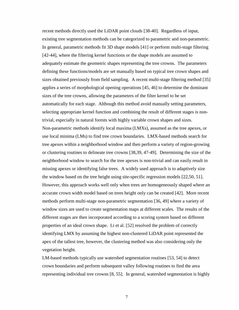
recent methods directly used the LiDAR point clouds [38-40]. Regardless of input,
existing tree segmentation methods can be categorized to parametric and non-parametric.
In general, parametric methods fit 3D shape models [41] or perform multi-stage filtering
[42-44], where the filtering kernel functions or the shape models are assumed to
adequately estimate the geometric shapes representing the tree crowns. The parameters
defining these functions/models are set manually based on typical tree crown shapes and
sizes obtained previously from field sampling. A recent multi-stage filtering method [35]
applies a series of morphological opening operations [45, 46] to determine the dominant
sizes of the tree crowns, allowing the parameters of the filter kernel to be set
automatically for each stage. Although this method avoid manually setting parameters,
selecting appropriate kernel function and combining the result of different stages is non-
trivial, especially in natural forests with highly variable crown shapes and sizes.
Non-parametric methods identify local maxima (LMXs), assumed as the tree apexes, or
use local minima (LMs) to find tree crown boundaries. LMX-based methods search for
tree apexes within a neighborhood window and then perform a variety of region-growing
or clustering routines to delineate tree crowns [38,39, 47-49]. Determining the size of the
neighborhood window to search for the tree apexes is non-trivial and can easily result in
missing apexes or identifying false trees. A widely used approach is to adaptively size
the window based on the tree height using site-specific regression models [22,50, 51].
However, this approach works well only when trees are homogeneously shaped where an
accurate crown width model based on trees height only can be created [42]. More recent
methods perform multi-stage non-parametric segmentation [36, 49] where a variety of
window sizes are used to create segmentation maps at different scales. The results of the
different stages are then incorporated according to a scoring system based on different
properties of an ideal crown shape. Li et al. [52] resolved the problem of correctly
identifying LMX by assuming the highest non-clustered LiDAR point represented the
apex of the tallest tree, however, the clustering method was also considering only the
vegetation height.
LM-based methods typically use watershed segmentation routines [53, 54] to detect
crown boundaries and perform subsequent valley following routines to find the area
representing individual tree crowns [8, 55]. In general, watershed segmentation is highly

8
prone to under/over-segmentation due to differences in tree heights and natural variability
of vegetation within tree crowns. To overcome this problem, studies use marker-
controlled watershed segmentation routines [56], where the basic idea is to mark the trees
and guide the watershed procedure to only delineate those marked trees. Marking
manually [22] is impractical for large-scale data. Automated approaches have generally
marked the tree apexes by performing morphological image analysis [57]. Similar to
LMX-based methods, these automated approaches are prone to missing tree apexes or
identifying false ones, especially when trees are not homogeneously shaped and sized.
Several methods have used a combination of apex identification (LMX-based) and
watershed segmentations (LM-based) to perform crown delineation and thus improve tree
detection rates [22,35,57,58].
2.2 Research materials
2.2.1 Study site
The study site of this dissertation research is the University of Kentucky Robinson Forest
(Lat. 37.4611, Long. -83.1555), a ~7,400 ha research forest located in the rugged eastern
section of the Cumberland Plateau region of southeastern Kentucky in Breathitt, Perry
and Knott counties (Figure 2.1). Terrain across Robinson Forest is characterized by a
branching drainage pattern, creating narrow ridges with sandstone and siltstone rock
formations, curving valleys and benched slopes. The slopes are dissected with many
intermittent streams [59], and are moderately steep ranging from 10 to over 100% facings
predominately northwest to south east and elevations ranging from 252 to 503 meters
above sea level (Figure 2.1).

9
Figure 2.1. Terrain relief map of the University of Kentucky Robinson Forest and its
general location within Kentucky, USA.
Vegetation in Robinson Forest features a diverse contiguous mixed mesophytic canopy,
which is made up of approximately 80 tree species with northern red oak (Quercus
rubra), white oak (Quercus alba), yellow-poplar (Liriodendron tulipifera), American
beech (Fagus grandifolia), eastern hemlock (Tsuga canadensis) and sugar maple (Acer
saccharum) as overstory species, while understory species include eastern redbud (Cercis
canadensis), flowering dogwood (Cornus florida), spicebush (Lindera benzoin), pawpaw
(Asimina triloba), umbrella magnolia (Magnolia tripetala), and bigleaf magnolia
(Magnolia macrophylla) [59, 60]. Average canopy cover across Robinson Forest is about
93% with small opening scattered throughout. Most areas exceed 97% canopy cover and
recently harvested areas have an average cover as low as 63% (Figure 2.2).

10
Figure 2.2. Aerial image of the camp and a glimpse over the canopy at Robinson Forest
in Clayhole, KY ccaptured in August 2016 (credit: Matt Barton, Agricultural Communications Services – University of Kentucky).
After being extensively logged in the 1920’s, Robinson Forest is considered second
growth forest ranging from 80-100 years old, and is now protected from commercial
logging and mining activities, typical of the area [61].
2.2.2 Recent field survey
Throughout the entire RF, 271 regularly distributed (grid-wise every 384 m) circular
plots of 0.04 ha in size, centers of which were georeferenced with 5 m accuracy, were
field surveyed during the summer of 2013. Within each plot, DBH (cm), tree height (m),
species, crown class (dominant, co-dominant, intermediate, overtopped), tree status (live,
dead), and stem class (single, multiple) were recorded for all trees with DBH > than 12.5
cm. In addition, horizontal distance and azimuth from plot center to the face of each tree
at breast height were collected to create a stem map. Site variables including slope,
11
aspect, and slope position were also recorded for each plot. Table 2.1 shows a plot level
summary.
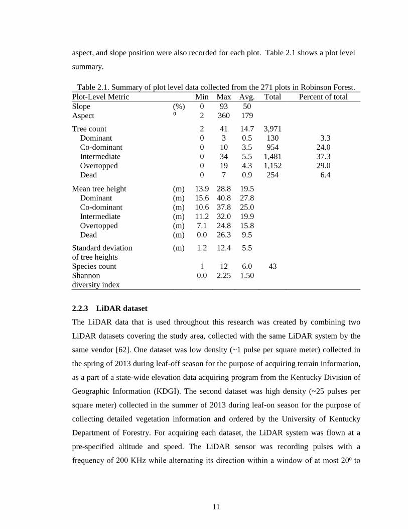
Table 2.1. Summary of plot level data collected from the 271 plots in Robinson Forest. Plot-Level Metric Min Max Avg. Total Percent of total Slope (%) 0 93 50 Aspect ⁰ 2 360 179
Tree count 2 41 14.7 3,971 Dominant 0 3 0.5 130 3.3 Co-dominant 0 10 3.5 954 24.0 Intermediate 0 34 5.5 1,481 37.3 Overtopped 0 19 4.3 1,152 29.0 Dead 0 7 0.9 254 6.4
Mean tree height (m) 13.9 28.8 19.5 Dominant (m) 15.6 40.8 27.8 Co-dominant (m) 10.6 37.8 25.0 Intermediate (m) 11.2 32.0 19.9 Overtopped (m) 7.1 24.8 15.8 Dead (m) 0.0 26.3 9.5
Standard deviation of tree heights
(m) 1.2 12.4 5.5
Species count 1 12 6.0 43 Shannon diversity index
0.0 2.25 1.50
2.2.3 LiDAR dataset
The LiDAR data that is used throughout this research was created by combining two
LiDAR datasets covering the study area, collected with the same LiDAR system by the
same vendor [62]. One dataset was low density (~1 pulse per square meter) collected in
the spring of 2013 during leaf-off season for the purpose of acquiring terrain information,
as a part of a state-wide elevation data acquiring program from the Kentucky Division of
Geographic Information (KDGI). The second dataset was high density (~25 pulses per
square meter) collected in the summer of 2013 during leaf-on season for the purpose of
collecting detailed vegetation information and ordered by the University of Kentucky
Department of Forestry. For acquiring each dataset, the LiDAR system was flown at a
pre-specified altitude and speed. The LiDAR sensor was recording pulses with a
frequency of 200 KHz while alternating its direction within a window of at most 20⁰ to

12
each side (40⁰ in total). The parameters of the LiDAR system and flight for both datasets
are presented in Table 2.2.
Table 2.2. LiDAR data acquisition parameters used for both datasets collected over
Robinson Forest. Leaf-Off Dataset Leaf-On Dataset Date of Acquisition April 23, 2013 May 28- 30, 2013 LiDAR System Leica ALS60 Leica ALS60 Average Flight Elevation above Ground 3,096 m 214 m Average Flight Speed 105 knots 105 knots Pulse Repetition Rate 200 KHz 200 KHz Field of View 40⁰ 40⁰ Swath Width 2,253.7 m 155.8 m Usable Center Portion of Swath 90% 95% Swath Overlap 50% 50% Maximum Returns per Pulse 3 4 Average Footprint 0.6 m 0.15 m Nominal Post Spacing 0.8 m 0.2 m
In addition to the 3D geographical coordinates of each point, the LiDAR system has
recorded the angle of the emitted pulse, the number of returns for each emission, the
return number and intensity of the returned pulse, which are also available in the datasets.
The vendor processed both raw LiDAR datasets using the TerraScan software [63] to
classify LiDAR points into ground and non-ground points. The LASTools extension [64]
in ArcMap 10.2 was used to create a combined LAS dataset file containing both LiDAR
datasets. Given the 50% swath overlap (doubling the total number of points within a
given area), multiple returns per pulse (slightly increasing the points), and using only 90–
95% of each swath (slightly reducing the number of points), the final density of the
combined dataset was at about 50 pt/m2. The vendor used the ground data points to create
a 1-meter resolution DEM using the nearest neighbor as the fill void method and the
average as the interpolation method.
2.3 Tree segmentation method
The proposed method is non-parametric and segments individual tree crowns based on
only the local information, crown shape and height of the vegetation, and does not require
a priori knowledge of either stand structure or typical tree attributes. A major

13
improvement of our approach, compared with existing approaches, is the dynamic
capture of local information about crown shape and its use to enhance crown
segmentation.
The main inputs of the tree segmentation method are the LiDAR point cloud and the
LiDAR-derived DEM. Independent of the point density, LiDAR point clouds have
variable, small-scale point spacing resulting from scan patterns (e.g., zig-zag) and flight
line overlap. Thus, a pre-processing routine is applied to homogenize point spacing.
This routine creates a grid with resolution equal to the average footprint (AFP), which
equals the reciprocal of square root of point density1, and filters the LiDAR point cloud
by selecting the highest elevation LiDAR point within each grid cell, hereafter called
LiDAR surface points (LSPs). Using the LiDAR-derived DEM, heights above ground
are calculated for all LSPs. Those LSPs below a minimum height, set here as 3 meter,
represent lower vegetation and are removed from further analysis. Based on the
vegetation structure (stem density and variability in tree heights), this creates several gaps
with no vegetation in the remaining LSP dataset, which is utilized later in the analysis.
The last pre-processing step smooths LSPs to reduce small variation in vegetation
elevation within tree crowns while maintaining important vegetation patterns. A Gaussian
smoothing filter with standard deviation equal to the AFP and a radius of 3×AFP was
used.
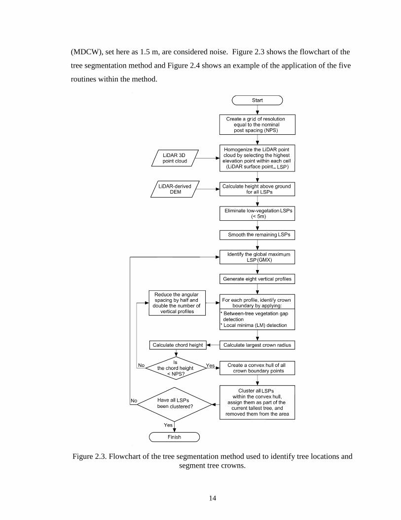
After the pre-processing steps, the tree segmentation method consists of the following
routines: 1) locate the global maximum elevation (GMX) amongst LSPs, which is
assumed to represent the apex of the tallest tree within a given area, 2) generate vertical
profiles originating from the GMX location and expanding outwards, 3) identify the
individual LSP along the profile that likely represents the crown boundary using
between-tree gap identification and LM identification for each profile, 4) create a convex
hull of boundary points, which delineates the tree crown, and 5) cluster all LSPs
encompassed within the convex hull and assign them as the current tallest tree crown.
This process is applied iteratively until all LSPs have been clustered into tree crowns.
Clusters representing crowns with diameter below a minimum detectable crown width
1 Number of points divided by the horizontal area covered by the points.
14
(MDCW), set here as 1.5 m, are considered noise. Figure 2.3 shows the flowchart of the
tree segmentation method and Figure 2.4 shows an example of the application of the five
routines within the method.
Figure 2.3. Flowchart of the tree segmentation method used to identify tree locations and
segment tree crowns.

15
Figure 2.4. Illustration of the preprocessing steps and the five routines within the tree
segmentation approach.

16
The most critical and non-trivial routines of the tree segmentation method are the
generation of an appropriate number of profiles and the identification of crown boundary
points to accurately segment tree crowns. The procedures developed for these two
routines form the basis for this novel tree segmentation method.
2.3.1 Profile generation
After identifying the GMX within a given area, vertical profiles originating from it and
expanding a maximum horizontal distance, set here to 15.24 m (50 feet), are generated.
The number of profiles required to smoothly represent tree crowns is determined
dynamically based on LiDAR-detected crown radii. The procedure starts with eight
uniformly spaced profiles (every 45°). After the crown boundary and thus radius is
determined for each profile (explained below), the maximum crown radius (r) is used to
determine the chord height (x) between two maximum crown radius profiles separated by
the angular spacing (φ) (Figure 2.5) as follows:
(1 ( / 2))x r cos ϕ= − 2.1
Figure 2.5. Diagram illustrating the calculation of the chord height (x) formed by two profiles of maximum crown radius (r) separated by the angular spacing (φ).
If the chord height is larger than AFP, the angular spacing is reduced by half and the
number of profiles is doubled. The new chord height is calculated again based on the
𝑟𝑟 𝑥𝑥 𝜑𝜑/2
𝑟𝑟
GMX
17
updated maximum crown radius and the new profile angular spacing. Doubling the
number of profiles continues iteratively until the chord height is smaller than AFP. By
using the maximum LiDAR-detected crown radius, the procedure ensures a sufficiently
large number of profiles and thus a smooth delineation of the tree crown.
The width of each profile was set to 2×AFP to ensure a sufficient number of LSPs
representing vegetation characteristics. Profiles are then analyzed vertically in two
dimensions using horizontal distance from the GMX and the elevation associated with
each LSP.
2.3.2 Crown boundary identification
After generating a vertical profile and identifying all LSPs along it, two sub-routines are
applied to identify the crown boundary. The first sub-routine identifies inter-tree crown
gaps via statistical analysis of the distribution of horizontal distances between
consecutive points along the profile. Thereafter, the second sub-routine inspects LM
points as potential crown boundaries based on the median slope of points within two
windows expanding both directions from each LM location.
2.3.2.1 Identification of inter-crown gaps
Figure 2.6-a shows a real example of a profile. We emphasize once more that points
below 3 m have already been excluded, resulting in relatively bigger horizontal distances
between some successive points in the profile. For each profile, we attempt to locate the
large horizontal gaps between any two successive points using the common Tukey
statistical outlier detection method [65]. The large gaps are an indication of gapping
between two crowns, where more LiDAR beams can penetrate toward the ground
recording more low vegetation points, which are already removed. The distances between
two successive points in a profile is Poisson distributed (Figure 2.6-b). Transforming a
Poisson distribution to its square root (or logarithm) yields a distribution that can
reasonably be approximated by a normal distribution [66], which is a more
straightforward distribution for different analyses especially for the Tukey outlier
detection procedure. Figure 2.6-c shows the square-root-transformed histogram, which
looks like a normal distribution except having some outliers on the right-hand side. The
major body of the histogram corresponds to the routine distances observed between any
two successive points on a tree crown. The close outliers in the right-hand side of the
18
histogram presumably correspond to distances between two points lying on a same tree
crown but with some little natural spacing observed in between. The farther outliers in
the histogram are very sparse. This part corresponds to extraordinary large gaps, which
are presumably the spacing between two different crowns.
Figure 2.6. a) A real example of a profile (a potential inter-crown gap is highlighted); b) Poisson distribution of the distances between any two successive point in the profile; c) square root Transformed distribution of the distances looking like a normal distribution for the major part (the outlier corresponding to the inter-crown gap is highlighted); d)
trimming the profile from the gaps on both sides of the GMX.
To be conservative, we trim each profile only from the extraordinary distances that are
very likely the inter-crown gaps. Any distance value that lies further than six times of the
Inter-Quartile Range (IQR) from the third quartile (Q3) is an extraordinary gap
(Figure 2.6-c). Starting from the GMX, we locate the first extraordinary gap and trim the
profile from there (Figure 2.6-d). Note that detecting the gaps is done merely on the local
statistics in a profile, rather than preset thresholds. This makes the detection of the gaps a
robust procedure irrespective of the tree species and formation as well as the DSM

19
attributes. However, looking for inter-crown gaps can only separate those crowns that
have a distinct gap in between, and is unable to separate tree crowns that are very close to
or overlap each other. However, trimming the profile from the first gap helps the analysis
of LMs be more straightforward, i.e., the sequence of points in a profile can hereafter be
assumed to correspond to adjacent tree crowns that are very close to each other or even
are overlapping. In other words, when considering an LM, we can now be fairly
confident that the sequences of points on both sides of the LM correspond to contiguous
high vegetation, whether they are from a single tree crown or from two immediate
crowns.
2.3.2.2 Identifying local minima points as crown boundaries
Starting from the GMX, this sub-routine identifies LM points defined as those with
elevations lower than their two adjacent neighbors. Once an LM point is found, the sub-
routine determines whether it represents the crown boundary or natural variation of
vegetation height within the crown. For this purpose, two windows expanding on both
sides of the LM are created. The left window considers all LSPs from the GMX to the
LM. The size of the right window is estimated based on the: i) steepness of consecutive
points within a distance equal to MDCW on the right of the LM, and ii) crown radii of
two hypothetical trees of equal height crowns of which represented by two distinctly
different shapes (a sphere and a narrow cone).
The steepness of LSPs on the right of the LM (Sright) is calculated as the median (in
degrees) of absolute slopes between consecutive points (i, i+1) within a distance of
MDCW from the LM (wMDCW):
( )1, 1 | , 1i iright rightS tan median slope i i MDCW−+
= + ∈∣
2.2
If the LM is in fact the crown boundary, the LSPs within wMDCW partially represent the
crown of an overlapping and shorter tree with a steepness that is approximated by Sright.
The value of Sright should range between the steepness of a sphere-shaped crown and the
steepness of a narrow cone-shaped crown (two ends of the spectrum). As the height of

20
the adjacent tree (had) is between the heights of the GMX and the LM point, its height is
reasonably approximated by the average of the GMX and the LM heights.
The steepness of a narrow cone-shaped crown can be expressed as 90°-ε, where ε (set
here as 5°) indicates a small deviation from vertical. The cone-shaped crown radius (crc)
can then be calculated as follows:
(90 )cad
c ch CLcr O
tan ε°×
= ×−
2.3
where CLc is the crown ratio, and Oc indicates the crown radius reduction due to the
overlap assuming the narrow cone-shaped tree is situated in a dense stand.
On the other hand, the slope of a sphere-shaped crown ranges from 0° to 90° with the
steepness (expected value) of 32.7° (see Appendix 2.A). Its crown radius (crs) can be
calculated as follows:
2sad
s sh CLcr O×
= ×
2.4
where, CLs and Os indicate the crown ratio and the crown radius reduction due to the
overlap within a dense stand for the sphere-shaped tree.
The size of the right window (wright) is then calculated by interpolating crc and crs with
respect to Sright, which should be bounded between 32.7° and 90°-ε, as follows:
(90 ) (90 )1
(90 ) 32.7 (90 ) 32.7right right
c srightS S
w cr crε εε ε
° °
° ° ° °
− − − −= + −
− − − −
2.5
Lastly, after determining both window sizes on either side of the LM, the median of
slopes between consecutive LSPs of each window is calculated. If the median slope of
the left-side window is negative (downwards from the apex to the crown boundary) and
the median slope of the right-side window is positive (upwards from the crown boundary

21
toward the apex of the adjacent tree crown), then the LM is considered a boundary point.
Otherwise, the current LM is considered to represent natural variation of vegetation
height within the current tallest tree crown and the next LM farther from the GMX along
the profile is evaluated. If none of the LMs found meet the crown boundary criterion
then the last LSP is considered as the crown boundary.
Crown ratio is highly variable among individual trees and species dependent with values
typically varying between 0.4 and 0.8 [67]. The crown ratio of a narrow cone-shaped tree
tends to be larger than that of a sphere-shaped one [68]. So, for the purpose of
illustrating the application of our method, we used 0.8 and 0.7 for CLc and CLs,
respectively. Similarly, crown radius reduction due to overlap is highly variable with a
value of less than 0.5 for a really dense stand. The radius of a narrow cone-shaped tree
tends to be reduced less than of a sphere-shaped tree because the crown of a narrow cone-
shaped tree is quite compact from the sides. So, we used two thirds for Oc and one third
for Os. Although the constant values set here can affect the final size determined for the
right window (Equation 2.5), the sign of the median slope would be the same as long as
the size is within a reasonable range. Still possible in practice, an excessively narrow
window might result in erroneously flipping the sign of the median slope and an LM
representing natural vegetation height within the crown to be misidentified as the crown
boundary and vice versa. However, when considering the multiple profiles generated for
each GMX, the effect of a single window size on the ability to delineate tree crown is
reduced.
Both sub-routines, to identify inter-tree gaps and crown boundaries respectively, are
completely based on the 3D positions of LSPs along a profile. This avoids prior
assumptions of tree crown shapes and dimensions, which makes the method robust
enough to be applied to different vegetation types.
2.4 Evaluation
In this section, we present the field data that is used to ground truth the proposed
segmentation method and then describe the evaluation procedure.
2.4.1 Ground truth field data
Within the Clemons Fork watershed (which covers an area of about 1,500 ha), 1.2×1.2
meter plywood boards, painted white to increase reflectance were installed prior to the

22
acquisition of LiDAR data at 103 of the 271 field plots. Boards were installed, leveled
with their centers placed at the exact location of the plot rebar markers, with the purpose
of more accurately geo-referencing the location of plot centers. After visually inspecting
LiDAR ground points and intensity values, boards (and thus plot centers) were clearly
identified for only 23 permanent plots, which were considered for the evaluation of the
tree-segmentation method. Although the location of the remaining plots could be
estimated by triangulation to clearly visible objects on the ground and the LiDAR data
(e.g., large trees, rock formations, vegetation gaps, road features), they were not
considered in the analysis to avoid mismatching exact plot locations and thus obscuring
comparisons between the tree-segmentation method and the field-collected data. Plots
were located on all aspect orientations and on slopes ranging from 10% to 70%. An
average of 13.2 trees were tallies per plot, with an average species diversity index [69] of
1.47 (Table 2.3). The LiDAR point cloud over each plot included a 5-m buffer for
capturing complete crowns of border trees.
Table 2.3. Summary of plot level data collected from the 23 accurately georeferenced plots in Robinson Forest.
Plot-Level Metric Min Max Average Total Percent of total Slope (%) 10 70 41 Aspect ⁰ 16 359 185 Tree count 6 27 13.2 303 Dominant 0 3 0.6 14 4.6 Co-dominant 0 10 3.4 78 25.7 Intermediate 2 10 5.5 126 41.6 Overtopped 0 15 3.1 72 23.8 Dead 0 5 0.6 13 4.3 Species count
3 9 5.6 33
Shannon diversity index
0.8 2.01 1.47
Median tree height
(m) 13.0 24.7 18.3
Interquartile range of tree heights
(m) 2.6 8.8 5.5
23
2.4.2 Evaluation procedure
To evaluate the performance of the tree segmentation method, we compared the location
of trees in the stem map created from field collected data with the location of LiDAR-
derived tree locations. As stump locations seldom coincide with the location of the
crown apexes (LiDAR-derived tree locations) due to leaning and irregular crown shape,
the exact coordinates from the stem map were not used in the evaluation. Instead, we
improved the tree detection evaluation procedure used by Kaartinen et al. [23]. A
LiDAR-derived tree location matches with a stem map location if: i) the angle between
the vertical projection of the 3D coordinates of the stump location and the 3D coordinates
of the LiDAR-detected apex is within a given leaning threshold, and ii) the height
difference is within a given threshold. If more than one LiDAR-derived tree location
match with a stem map location or vice versa, only the best one is used.
A scoring system was developed to match multiple LiDAR-derived tree locations with
the most appropriate stem map location. Three increasing leaning (5°, 10°, and 15°) and
height difference (10%, 20%, and 30%) threshold levels with decreasing scores (100, 70,
and 40) were considered (Table 2.4, Figure 2.7). A matrix with matching scores for all
possible pairs of LiDAR-derived tree locations (rows) and stem map locations (columns)
was then constructed. It was then processed by the Hungarian assignment algorithm [70]
to produce the optimal matching assignment with the greatest total matching score.
Table 2.4. Leaning and height difference thresholds with associated scores considered for matching LiDAR-derived tree locations to stem map locations.
Leaning threshold (⁰)
Height difference threshold (%)
Score
5 10 100 10 20 70 15 30 40 > > 0
24
Figure 2.7. Calculation of leaning angle and distance difference used in the matching
score system.
In the optimal assignment, a matched tree is an assigned pair of a LiDAR-derived tree
location and a stem map location. An omission is a stem map location that remains
unassigned (score=0). A commission is an unassigned LiDAR-derived tree location. The
number of matched trees (MT) is an indication of the segmentation quality. The number
of omission errors (OE) and commission errors (CE) indicate under- and over-
segmentation, respectively. The accuracy of the approach was calculated in terms of
recall (Re), precision (Pr) and F-score (F) using the following equations [71]:
MTRe MT OE=+
2.6
MTPr MT CE=+
2.7
2 Re PrF Re Pr× ×=
+
2.8

25
Recall is a measure of the tree detection rate, precision is a measure of correctness of
detected trees and the F-score indicates the overall accuracy taking omission and
commission errors into account.
2.5 Results and discussion
2.5.1 Segmentation accuracy
The accuracy of the tree-segmentation approach on trees in the 23 plots is presented in
Table 2.5. On average, the tree detection rate of the segmentation approach was 72%,
and 86% of detected trees were correctly detected. The overall accuracy in terms of the
F-score was 77%. Recall values ranged from 31% to 100% and precision values ranged
from 50% to 100%. In dense plots with a relatively large number of intermediate and
overtopped trees, several trees were under-segmented resulting in relatively low recall
values. For example, 6 of 19 and 0 of 11 intermediate and overtopped trees were
detected in plots 4 and 11, respectively. However, all dominant and co-dominant trees in
these two plots were detected. As expected, the three accuracy metrics were higher for
dominant and co-dominant trees compared with intermediate and overtopped trees
(Table 2.5). Recall increased to 94% for larger trees and decreased to 62% for smaller
trees. Precision was more stable; it changed slightly about 1% from the overall 86%,
87% for larger trees and 85% for smaller trees. When considering all trees, the tree-
segmentation approach was able to detect 100% of dominant, 92% of co-dominant, 74%
of intermediate, and 38% of overtopped trees in the 23 plots. In addition, the approach
was able to detect 39% of dead trees (Table 2.5).

Table 2.5. Summary of accuracy results of the tree segmentation approach on the 23 plots.
Plot
Number of Lidar detected / Field measured by tree class
Total number of matches and errors
Overall accuracy (%)
Accuracy by tree class group (%) D & C I, O, & Dead
D1 C2 I3 O4 Dead MT5 OE6 CE7 Re8 Pr9 F10 Re Pr F Re Pr F 1 0/0 3/3 6/10 1/3 0/0 10 6 3 62.5 76.9 69.0 100.0 75.0 85.7 53.8 77.8 63.6 2 1/1 3/3 4/4 2/6 0/0 10 4 1 71.4 90.9 80.0 100.0 100.0 100.0 60.0 85.7 70.6 3 0/0 3/3 4/4 0/5 0/1 7 6 1 53.8 87.5 66.6 100.0 75.0 85.7 40.0 100.0 57.1 4 1/1 4/4 ¾ 3/15 2/3 13 14 0 48.1 100.0 65.0 100.0 100.0 100.0 36.4 100.0 53.3 5 1/1 4/4 9/9 6/7 0/0 20 1 0 95.2 100.0 97.5 100.0 100.0 100.0 93.8 100.0 96.8 6 2/2 ½ 3/3 0/0 0/0 6 1 1 85.7 85.7 85.7 75.0 100.0 85.7 100.0 75.0 85.7 7 0/0 9/10 2/8 0/3 0/0 11 10 4 52.4 73.3 61.1 90.0 75.0 81.8 18.2 66.7 28.6 8 1/1 5/6 5/8 0/1 0/0 11 5 1 68.8 91.7 78.6 85.7 85.7 85.7 55.6 100.0 71.4 9 0/0 2/2 7/9 2/3 0/0 11 3 1 78.6 91.7 84.6 100.0 66.7 80.0 75.0 100.0 85.7
10 0/0 1/1 2/2 3/6 1/5 7 7 0 50.0 100.0 66.7 100.0 100.0 100.0 46.2 100.0 63.2 11 1/1 4/4 0/8 0/3 0/0 5 11 2 31.3 71.4 43.5 100.0 71.4 83.3 00.0 00.0 00.0 12 0/0 4/4 ¾ 2/3 0/0 9 2 4 81.8 69.2 75.0 100.0 57.1 72.7 71.4 83.3 76.9 13 0/0 3/3 7/7 0/0 0/0 10 0 1 100.0 90.9 95.2 100.0 100.0 100.0 100.0 87.5 93.3 14 0/0 2/2 3/3 1/1 0/0 6 0 0 100.0 100.0 100.0 100.0 100.0 100.0 100.0 100.0 100.0 15 0/0 9/9 3/3 0/0 0/1 12 1 2 92.3 85.7 88.9 100.0 81.8 90.0 75.0 100.0 85.7 16 1/1 ½ 5/8 3/6 0/0 10 7 0 58.8 100.0 74.1 66.7 100.0 80.0 57.1 100.0 72.7 17 0/0 4/4 6/6 2/2 1/1 13 0 4 100.0 76.5 86.7 100.0 66.7 80.0 100.0 81.8 90.0 18 3/3 0/0 1/3 0/0 0/0 4 2 1 66.7 80.0 72.7 100.0 100.0 100.0 33.3 50.0 40.0 19 2/2 0/2 2/4 0/1 0/0 4 5 4 44.4 50.0 47.0 50.0 66.7 57.1 40.0 40.0 40.0 20 0/0 2/2 4/6 0/0 0/0 6 2 2 75.0 75.0 75.0 100.0 100.0 100.0 66.7 66.7 66.7 21 0/0 2/2 4/5 2/4 1/1 9 3 0 75.0 100.0 85.7 100.0 100.0 100.0 70.0 100.0 82.4 22 1/1 1/1 6/6 0/1 0/1 8 2 0 80.0 100.0 88.9 100.0 100.0 100.0 75.0 100.0 85.7 23 0/0 5/5 2/2 0/2 0/0 7 2 3 77.8 70.0 73.7 100.0 83.3 90.9 50.0 50.0 50.0
Average detection
14/14 100%
72/78 92.3%
93/126 73.8%
27/72 37.5%
5/13 38.6%
206/303 68.0%
94/303 31.1%
35/303 11.6%
71.7 85.5 76.7 94.2 87.1 89.5 61.6 84.7 70.9
1 Dominant, 2 Co-dominant, 3 Intermediate, 4 Overtopped 5 Matched Trees, 6 Omission Errors, 7 Commission Errors, 8 Recall, 9 Precision, 10 F-score
26

27
As an example, Figure 2.8 shows the results of the tree segmentation performance for
plot 8, 14, 15, and 22. Empty areas close to plot boundaries represent crowns of non-
matched trees outside the plots (apex is outside of the boundary), which were removed
from the analysis. Omissions in these empty areas (i.e., lower right side of plot 8) are
intermediate and overtopped trees likely below dominant trees outside the plot boundary.
As the LiDAR point clouds include buffer areas, several matched tree crowns extend
beyond the plot boundary. Many crowns do not look circular because of the dense
canopies and the fact that the crowns may be undercover to some extent. Two
commissions can be observed in plot 15 where nine co-dominant trees are growing
tightly in a small area.

28
Figure 2.8. Aerial visualization of the tree segmentation results in four plots within the
study area. Distinct colors represent matched tree crowns.
2.5.2 Applicability to different conditions
We evaluated relationships between accuracy metrics for each tree group (precision,
recall, and F-score) and plot level attributes, i.e., average terrain slope, tree density,
species diversity index, percentage of dominant, co-dominant, intermediate, overtopped,
and dead trees, as well as median and interquartile range of tree heights (IQRH). None of
the relationships for dominant and co-dominant group of trees was statistically

29
significant. For the smaller group of trees, we observed negative correlations between
recall and IQRH (P=.004, R²=.33) and diversity index (P=.03, R²=.2). Similarly, there
was a negative correlation between F-score and IQRH (P=.03, R²=.21). Also, a negative
correlation between precision and percentage of dominant trees (P=.02, R²=.24) was
observed. These correlations verify that in multi-story plots with large dominant trees,
intermediate and overtopped trees are more difficult to detect. As the tree segmentation
method considers only LSPs, dominant and co-dominant trees can be easily detected. On
the other hand, the crowns of intermediate and overtopped trees are only partially visible
from above and in some cases completely underneath large tree crowns, making them
harder to be detected. The correlations we observed between accuracy metrics and plot
level attributes are weak and insignificant specially for larger group of trees, which likely
indicates that the accuracy of the tree-segmentation approach is not sensitive to
differences in stand and terrain structures of the study area. This demonstrates the
robustness of the approach and increases its potential applications.
Other tree-segmentation studies in closed-canopy deciduous forests have reported tree
detection accuracies of about 50% [21, 72], 65% [35], and 72% [58] using similar
evaluation metrics, which take both omissions and commissions into account.
Vauhkonen et al. [26] compared six different single tree detection methods on two
deciduous forest sites. Performances were similar across sites; the average F-score of all
methods was 57% where the maximum F-score was 64% and average recall and
precision were 47% and 74%, respectively. Also, Duncanson et al. [73] used a
multilayered crown delineation approach, which correctly identified 70% of dominant
trees, 58% of co-dominant trees, 35% of intermediate trees, and 21% of overtopped trees
in a deciduous forest. Tree-segmentation accuracies from these previous studies in
deciduous forests are slightly lower than the accuracy from our novel approach, which is
an indicator of potential applicability of our study to deciduous forests with complex
vegetation conditions.
2.6 Conclusion
Developing automated approaches to obtain tree-level information over large forested
areas is increasingly important for accurate assessment, monitoring and management.
Most of existing methods are forest type specific and applied to conifer forests. In this

30
chapter, we presented a generic tree segmentation method that uses small foot print
LiDAR data and applied it to natural deciduous forests with complex structures. A
significant advantage of our novel approach is that it does not require a priori knowledge
of tree shapes and sizes. The approach retrieves local information, crown steepness and
height of the vegetation, and uses it on-the-fly to enhance the crown segmentation.
Using an improved evaluation method, results showed that our approach was able to
detect 72% of trees, and 86% of detected trees were correctly identified, resulting in an
overall accuracy of 77%. Examining results by crown class, the method detected 94% of
dominant and co-dominant trees and 62% of intermediate and overtopped trees.
Statistical analysis revealed similar accuracy levels across plots with different structures,
which indicates the potential successful application of our method to other forest types.
The main research challenge of the proposed tree segmentation method was capturing
heterogeneously shaped trees, and detecting intermediate and overtopped trees that may
entirely be non-present within LSPs was not attempted explicitly. Next chapter will focus
on presentation of a vertical stratification method that decomposes the LiDAR point
cloud to an overstory and multiple understory canopy layers, thereby improving the
detection rate of understory trees.

31
2.A. Expected slope of a spherical surface
The slope of a spherical surface in degrees ranges between 0-90° (Figure 2.9). Assuming
the LiDAR surface points are uniformly distributed along the horizontal dimension, the
expected value of the slope (α) is calculated as follows.
1 10
. 1 32.72pisin x dxα − °= = − =∫
2.9
Figure 2.9. The angle α representing the slope of the unit circle is a function of x.
Copyright © Hamid Hamraz 2018

32
3 Vertical Stratification
Due to the ability to penetrate vegetation canopy, LiDAR 3D point clouds also contain
vertical information from which vegetation structural information can be retrieved [5, 74-
76]. This structural information may also include understory layers, which is of great
value for various forestry applications and ecological studies [77-80]. Although
understory trees provide limited financial value and form a minor proportion of total
above ground biomass, they influence canopy succession and stand development, create a
heterogeneous and dynamic habitat for numerous wildlife species, and are an essential
component of forest ecosystems [25, 81, 82]. However, to obtain individual tree
attributes (e.g., location, crown width, height, DBH, volume, biomass) from different
canopy layers, accurate and automated tree segmentation approaches that are able to
separate tree crowns both vertically and horizontally are required [40, 73, 83, 84].
Nevertheless, tree detection rate of understory trees (typically below 60%) is consistently
lower than overstory trees (typically around or above 90%) [36, 85]. The major reason of
this deficiency is the occlusion effect of higher vegetation layers that considerably
decrease the penetration of LiDAR pulses toward lower layers. This fact results in much
lower point density representing understory trees [24, 75, 76, 86, 87]. Although
variability in stand structure and terrain condition is the major factor affecting tree
segmentation quality [23, 88, 89], a minimum point density is the basic requirement for
reasonable segmentation of trees [27, 28, 90]. However, this basic requirement is
typically not satisfied for understory trees in a dense forest due to occlusion [85, 91].
To improve detection of understory trees, in this chapter, we present a method that
stratifies the LiDAR point cloud of a forest canopy to an overstory and multiple
understory canopy layers by analyzing vertical distributions of LiDAR points [92]. To
further investigate the subpar detection rate of understory trees, , we then present a
canopy occlusion model by inspecting how the point density of canopy layers decrease
with proximity to the ground [93]. In Section 3.1, we review the related literature.
Section 3.2 is devoted to description of the vertical stratification method and the canopy
occlusion model. In Section 3.3, we present the results where tree segmentation
accuracies with and without vertical stratification are compared, statistics of the stratified

33
canopy layers are summarized, and estimates using the occlusion model are provided.
We present discussions in Section 3.4 and lastly Section 3.5 concludes the chapter.
3.1 Literature review
Numerous methods for individual tree segmentation within LiDAR data have been
developed. Earlier methods use pre-processed data in the form of DSMs or CHMs to
segment individual trees [21, 35, 49, 51, 57]. These methods have an inherent drawback
of missing understory trees by considering only the surface data [37, 40]. More recent
methods process the raw point clouds in order to utilize all horizontal and vertical
information and, from the computational viewpoint, can be classified to volumetric or
profiler methods. Volumetric methods directly search the 3D volume for the individual
trees [36, 52, 83, 94-99]. For example, Ferraz et al. [83] used the mean shift clustering to
segment the point cloud and assigned each segment to overstory, understory, or ground
vegetation layer. Véga et al. [36] performed segmentations at different scales and used
criteria based on the shape of an ideal tree crown to dynamically select the best set of
apices. Sačkov et al. [99] developed a moving window analysis method to identify
potential apices and used several tree allometry rules to increase the likelihood of
detecting the actual tree profiles. However, volumetric methods are generally
computationally intensive and may be prone to suboptimal solutions due to the large
magnitude of the search space.
On the other hand, profiler methods reduce the computational load through a modular
process. They typically have a module for vertical segmentation (i.e., to strip the 3D
volume to multiple 2D horizontal profiles), a module for horizontal segmentation (i.e., to
search the trees within the profiles), and a module to ultimately aggregate the results
across the profiles [100]. However, these methods generally lose information about the
vertical crown geometry when processing a 2D profile. To minimize information loss
due to profiling, other profiler methods have analyzed vertical distribution of LiDAR
points to identify 2.5D profiles embodying more information about vertical crown
geometry. Wang et al. [40] searched trees within each profile and used a top-down
routine to unify any detected crowns that may be present in different profiles. They
analyzed vertical distribution of all LiDAR points globally within a given area to
determine the height levels for stripping profiles. However, depending on the vegetation

34
height variability, a globally derived height level may lead to under/over-segmenting tree
crowns across the profiles. Other approaches addressed this issue by identifying
constrained regions including one or more trees using a preliminary segmentation routine
and independently 2.5D profiling each region [73, 101, 102], yet the final result is
dependent on the preliminary segmentation.
Very few studies have analysed the occlusion effect because of the vegetation density.
Kükenbrink, Schneider [24] have recently quantified the occlusion effect of higher
canopy layer on lower layers and reported that at least 25% of canopy volume remain
uncovered even in small-footprint LiDAR acquisition campaigns. They suggested
increasing flight strip overlap, adding more observation angles and increasing point
density, to uncover more of the canopy, yet they did not considered the occlusion effect
on segmentation quality of individual trees.
3.2 Methods
3.2.1 Vertical stratification of canopy
The method vertically stratifies the point cloud to 2.5D profiles, hereafter referred to as
canopy layers, by iteratively removing the top canopy layer until the point cloud is
emptied. Each canopy layer is sensitive to stand height variability and includes a layer of
non-overtopping tree crowns within an unconstrained area. To stratify the top canopy
layer, the point cloud is binned into a horizontal grid with a cell width equal to the AFP
(as layers are removed from the point cloud, point density decreases and AFP increases).
The height threshold for removing the top layer is determined independently per each
grid cell by inspecting the height histogram of all points in a circular locale around the
cell. The locale should include sufficient number of points for building an empirical
multi-modal distribution but not extending very far to preserve locality. We fixed the
radius of the locale to 6×AFP (essentially containing about π×6² points) and lower
bounded it at 1.5 m to prohibit too small locales capturing insufficient spatial structure.
To process a locale, we create a height histogram (bins fixed at 25 cm) of the points in
the locale and smooth the histogram to remove variabilities pertaining to vertical
structure of a single crown. We used a Gaussian filter with a standard deviation fixed at
5 m for smoothing. Every salient curve in the smoothed histogram, corresponding to a
sequence of histogram bins throughout which the second derivative is negative,

35
represents a canopy layer [40, 101]. We choose the mid-point of the gap between the top
layer and the second top layer as the height threshold for removing the top canopy layer
within the cell location (Figure 3.1).
Figure 3.1. Height histogram of LiDAR points within a locale including over 100 points
used for determining the height threshold for removing the top canopy layer in a cell location.
The height thresholds for removing the top canopy layer are determined using
overlapping locales without a priori assumptions about tree crown shape or size. Hence,
the canopy layer smoothly adjusts to incorporate vertical variabilities of crowns within an
unconstrained area to minimize under/over-segmenting tree crowns. After vertical
stratification, individual tree crowns can be segmented by applying the method presented
in the previous chapter independently to each canopy layer. Because the segmentation
method also does not make a priori assumptions about the stand structure, the
combination is a robust tree segmentation approach for a multi-layered stand that can be
applied to different forest types. Figure 3.2 illustrates segmentation of a multistory stand using
the vertical stratification and the individual crown segmentation methods combined together. As

36
can be seen in Figure 3.2, a number of understory trees seem to be missed within the third
canopy layer, which is likely due to the much lower point density compared to the first
and second layers.
We evaluated the accuracy of the segmentation with and without canopy stratification
over the 271 field surveyed plots (Table 2.1) to assess the utility of the canopy
stratification procedure. We conducted two-tailed paired T-tests to compare the DSM-
based and the stratification-enabled approach over nine accuracy metrics, i.e., precision,
recall, and F-score (Equations 2.6, 2.7, and 2.8) for overstory (dominant and co-
dominant), understory (intermediate and overtopped), and all trees. Our sample of 271
plots is large enough to satisfy the assumptions of the T-test even if the data is not
normally distributed. We also inspected the Pearson correlations of the accuracy metrics
for the stratification-enabled approach with different plot level parameters. These
correlation relations help investigate how the performance of the approach is affected
according to the terrain and stand variability across Robinson Forest.
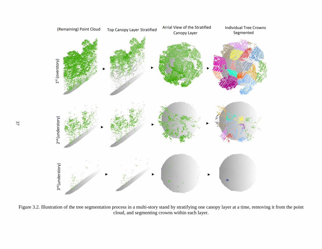
Figure 3.2. Illustration of the tree segmentation process in a multi-story stand by stratifying one canopy layer at a time, removing it from the point
cloud, and segmenting crowns within each layer.
37

38
3.2.2 Canopy occlusion model
Assuming all canopy layers cover the same area as the entire point cloud, the point
density of the entire cloud (PCD) equals the sum of point densities of constituting canopy
layers plus the density of the DEM representing the bare ground. Because the ground is
different from a canopy layer in interaction with LiDAR pulses, necessitating a different
density model for the DEM, we assume an infinite number of canopy layers were placed
instead of the ground to simplify the analysis. Point density of the DEM approximately
equals the total of point densities of the canopy layers in place of the ground. Hence
PCD can be calculated as the sum of point densities of an infinite number of canopy
layers (the actual ones plus those in place of the ground):
1 2 3 nPCD d d d d n= + + +…+ ∈ 3.1
where dn denotes the point density of the nth canopy layer, which converges to zero as n
increases because point density of individual canopy layers generally decreases with
proximity to ground level (Figure 3.2) [85, 103, 104]. To normalize point densities, we
divide both sides of Equation 3.1 by PCD:
1 2 31 np p p p n= + + +…+ ∈ 3.2
where pn denotes the fraction of LiDAR points at the nth layer that can be estimated using
a probability distribution function (bearing the property of summation to one).
We denote the required PCD of a point cloud for a reasonable segmentation of trees
forming the top canopy layer of the point cloud by PCDmin. The required PCD of a point
cloud for a reasonable segmentation of trees forming the nth canopy layer can then be
calculated using Equation 3.2. We hypothetically remove the n-1 top canopy layers of the
point cloud. The resulting point cloud would have a density fraction of 1 - (p1+p2+...+pn-
1) of the original point cloud. Assuming this density fraction yields a density of PCDmin
for the resulting point cloud, the point density of the original point cloud for a reasonable
segmentation of trees forming its nth top canopy layer (pcdmin(n)) by proportionality
becomes:

39
1 2 1( ) 1 ( )
minmin
n
PCDpcd n p p p −=
− + +…+
3.3
In order to estimate pn (Equation 3.3), we conducted a data-driven study. We created a
regularly distributed sample (40 m spacing) of 50,911 circular (radius = 15 m) plot point
clouds from the entire Robinson Forest data. We then vertically stratified each point
cloud to its canopy layers. Each layer completely below a minimum height of 3 m was
likely associated with ground level vegetation and was not regarded as a canopy layer. A
canopy layer may however extend below this minimum height and even touch the
ground. We recorded a sequence of five pn values (1 ≤ n ≤ 5 – zeros for missing layers)
per each sample point cloud with at least one canopy layer. We then fitted a logarithmic
series distribution [105] (having a discrete decreasing function supporting natural
numbers) to all (n, pn) pairs.
We conducted another data-driven study in order to estimate PCDmin. We decimated the
point cloud to simulate a PCD of 1–50 pt/m². For each desired PCD value, we binned the
point cloud into a horizontal grid with cell width of the equivalent AFP. We then
randomly selected a first return point within each cell and kept all returns associated with
the LiDAR pulse generating that first return [27, 106]. We then vertically stratified the
point clouds of the 23 accurately georeferenced plots in Robinson Forest (Table 2.3) to
their canopy layers, and segmented individual tree crowns within those layers. Lastly, we
inspected the tree segmentation accuracies for overstory and understory trees as a
function of point density. The point density at which segmentation accuracies of
overstory trees plateau is regarded as PCDmin.
3.3 Results
3.3.1 Segmentation accuracy On average for the 271 sample plots, results from the tree segmentation method without vertical
stratification show higher precisions by 5–15% while the stratification-enabled approach shows
higher recalls by 5–22% and higher F-scores by up to 12% (Figure 3.3). When comparing the
stratification-enabled against the basic method using T-tests (Table 3.1), all metrics except F-
score for overstory trees showed significant (P < 0.0001) changes. Recall and precision
for understory trees showed the largest changes: an increase from 46% to 68% (MSE =

40
10.04) and a decrease from 99% to 84% (MSE = 3.97), respectively. Overall, the
stratification-enabled tree segmentation method shows improvements in F-scores for
understory (from 61% to 73%, MSE = 1.70) as well as all trees (from 70% to 77%, MSE
= 0.66), while barely affecting F-score for overstory trees compared with the basic
approach (Figure 3.3).

41
Figure 3.3. Average segmentation accuracies over the 271 sample plots grouped by
crown class.
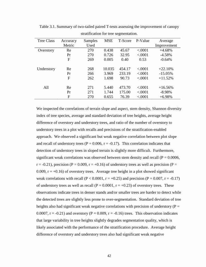
42
Table 3.1. Summary of two-tailed paired T-tests assessing the improvement of canopy
stratification for tree segmentation.
Tree Class Accuracy Metric
Samples Used
MSE T-Score P-Value Average Improvement
Overstory Re 270 0.438 45.67 <.0001 +4.68% Pr 270 0.726 32.95 <.0001 -4.58% F 269 0.005 0.40 0.53 -0.64%
Understory Re 268 10.035 454.17 <.0001 +22.10% Pr 266 3.969 233.19 <.0001 -15.05% F 262 1.698 90.73 <.0001 +11.52%
All Re 271 5.440 473.70 <.0001 +16.56%
Pr 271 1.744 175.00 <.0001 -8.98% F 270 0.655 76.39 <.0001 +6.98%
We inspected the correlations of terrain slope and aspect, stem density, Shannon diversity
index of tree species, average and standard deviation of tree heights, average height
difference of overstory and understory trees, and ratio of the number of overstory to
understory trees in a plot with recalls and precisions of the stratification-enabled
approach. We observed a significant but weak negative correlation between plot slope
and recall of understory trees (P = 0.006, r = -0.17). This correlation indicates that
detection of understory trees in sloped terrain is slightly more difficult. Furthermore,
significant weak correlations was observed between stem density and recall (P = 0.0006,
r = -0.21), precision (P = 0.009, r = +0.16) of understory trees as well as precision (P =
0.009, r = +0.16) of overstory trees. Average tree height in a plot showed significant
weak correlations with recall (P < 0.0001, r = +0.25) and precision (P = 0.007, r = -0.17)
of understory trees as well as recall (P = 0.0001, r = +0.23) of overstory trees. These
observations indicate trees in denser stands and/or smaller trees are harder to detect while
the detected trees are slightly less prone to over-segmentation. Standard deviation of tree
heights also had significant weak negative correlations with precision of understory (P =
0.0007, r = -0.21) and overstory (P = 0.009, r = -0.16) trees. This observation indicates
that large variability in tree heights slightly degrades segmentation quality, which is
likely associated with the performance of the stratification procedure. Average height
difference of overstory and understory trees also had significant weak negative

43
correlations with recall of understory trees (P = 0.002, r = -0.19) and precision of
overstory trees (P = 0.004, r = -0.18). This reaffirms the fact that smaller (understory)
trees are harder to detect and larger (overstory) trees are more prone to over-segmentation
while it also indicates the robustness of the stratification procedure because the tighter
gap between overstory and understory seemed not to degrade performance metrics.
Lastly, the ratio of overstory to understory trees showed a relatively stronger negative
correlation with precision of understory trees (P < 0.0001, r = -0.35). A larger number of
overstory trees means more occlusion for understory trees resulting in lower point density
and potentially less homogeneity in point distribution of understory canopy layers,
making understory trees more prone to over-segmentation. This observation is mainly
associated with the low point density of understory canopy layers rather than the
segmentation approach.
3.3.2 Stratified canopy layers
Within the 50,911 plot point clouds sampled from Robinson Forest data, the vertical
stratification method identified 0 layers for plots where no sufficiently large trees were
present, and up to 5 layers for plots with very complex canopy structures (Table 3.2).
Most plots had 3 (47.5%) or 4 (24.7%) canopy layers and the average number of canopy
layers were 2.76. We define starting height and thickness of a canopy layer as the
median over all grid cells used to stratify the layer (Figure 3.1). The average starting
height of a canopy layer ranged from 0.1 to 15.3 m and the average thickness of a layer
ranged between 5.6 and 8.4 m. Also, the average point density of a canopy layer ranged
between 0.06 and 44.52 pt/m². The average starting height, thickness, and point density
of the entire canopy (all layers aggregated) was 0.3 m, 20.9 m, and 48.1 pt/m²,
respectively. The average PCD of a plot (all canopy layers plus ground level vegetation
and DEM) was 50.5 pt/m², which agrees with the point density of the initial LiDAR
dataset (see Section 2.2.3 for details of the LiDAR dataset).

44
Table 3.2. Summary statistics of canopy layers over the 50,911 sample plots regularly distributed in Robinson Forest.
Canopy Layer Plots1
Starting Height (m)
Thickness (m) Point Density (pt/m²)
Avg. S.D. Avg. S.D. Avg. S.D. 1 5.86% 15.20 6.56 8.30 0.81 44.52 19.02
2 10.17% 3.76 2.80 8.39 1.20 7.03 4.29
3 47.50% 0.58 1.08 6.66 1.38 0.97 1.01
4 24.71% 0.31 1.12 6.06 1.54 0.41 0.83
5 1.76% 0.09 0.08 5.06 1.35 0.06 0.54
Aggregate 90.00% 0.31 0.47 20.93 9.03 48.09 23.33
1 Plots having as many number of canopy layers.
Thickness of a canopy layer seemed to be unrelated to its starting height except only for
very low starting heights (Figure 3.4), which is likely associated with layers formed by
very small trees. Dependence of a canopy layer thickness on the number of layers
preceding it and its independence to height is likely due to the fact that tree crowns within
a canopy layer adapt their shape to maximize light exposure [107, 108], and light
exposure is related to the amount of light already intercepted by preceding canopy layers
rather than the height of the layer.
Figure 3.4. Thickness of canopy layer according to starting height of the layer.
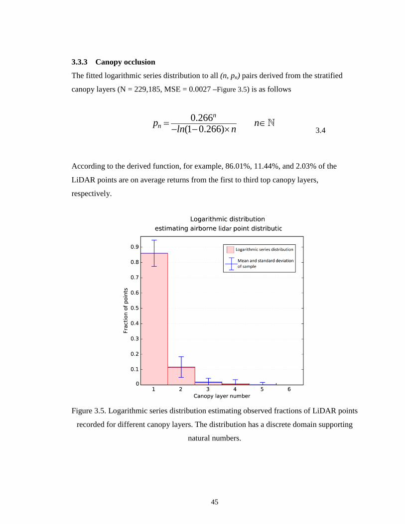
45
3.3.3 Canopy occlusion
The fitted logarithmic series distribution to all (n, pn) pairs derived from the stratified
canopy layers (N = 229,185, MSE = 0.0027 –Figure 3.5) is as follows
0.266(1 0.266)
nnp nln n= ∈
− − ×
3.4
According to the derived function, for example, 86.01%, 11.44%, and 2.03% of the
LiDAR points are on average returns from the first to third top canopy layers,
respectively.
Figure 3.5. Logarithmic series distribution estimating observed fractions of LiDAR points
recorded for different canopy layers. The distribution has a discrete domain supporting
natural numbers.

46
Figure 3.6 shows segmentation accuracies of overstory and understory trees as functions
of PCD. As shown for overstory trees, accuracy scores are relatively stable for PCD
values larger than 10 pt/m². Recall tends to decrease slightly, which is compensated by
slight increases in precision resulting in a stable F-score for PCD values between 4 and
10 pt/m². Recall and consequently F-score start dropping remarkably for PCD values
lower than 4 pt/m².
Figure 3.6. Accuracy scores of tree segmentation based on density of LiDAR point cloud
for overstory and understory trees.
The accuracy score trends of overstory trees concur with the previous work. As shown,
the accuracy scores plateau at about 4 pt/m² [27, 28, 90], which is assumed here as the
value for PCDmin. Using Equations 3.3, 3.4, the required PCD for a reasonable
segmentation of trees for as deep as three canopy layers (pcdmin(3)) would be 169.57

47
pt/m². This PCD approximates the required PCD to reasonably segment understory trees
because they are typically found in as deep as the third canopy layer [73, 83]. Similarly,
if we require a reasonable segmentation for as deep as only two canopy layers, the
minimum PCD (pcdmin(2)) becomes 30.07 pt/m².
3.4 Discussion
Although the stratification procedure is in theory robust and applicable to a variety of
stand structures, it increased the number of over-segmentations by a fair amount (5–15%)
depending on the crown class in our study. Inspecting Figure 3.1, vertical over-
segmentation is likely when the smoothing operation cannot remove the vertical
variability pertaining to a single crown. We tried to alleviate this problem by adaptively
adjusting the size of the smoothing window according to vegetation height so as to reach
a more favorable trade-off between under- and over-segmentations, yet our attempt did
not make improvements. We also tried a post-processing module to merge the likely
over-segmentations back to the crown they belong to, but this attempt also resulted in no
improvements. We speculate adjusting the window size based on the field observations
of a forested area in question is the best path to follow to tackle this problem. Overall, the stratification procedure improved tree segmentation accuracies (Figure 3.3,
Table 3.1). However, this overall improvement is majorly composed of a strong increase
in detection rate and a moderate decrease in correctness of the detected understory trees.
Detecting more trees likely increased the chance of over-segmentation of the detected
trees, and this was strongly pronounced for understory trees compared with overstory
trees. This observation indicates an increased sensitivity of the stratification-enabled
method to segment understory trees while barely affecting the segmentation of overstory
trees compared with the basic method, which is also an indication of the sound operation
of the stratification procedure. Correlations of the accuracy metrics with plot level
metrics over a forest with a complex and highly variable structure were insignificant
and/or weak. This observation evidences that the stratification-enabled approach can also
be used for multi-layered tree segmentation of different forest types.
To understand the vertical structure of tree canopy layers of forested landscapes [104,
109], the proposed stratification procedure can be applied independent of the tree
segmentation method. As observed, average thickness and point density decreases with

48
lower canopy layers (Table 3.2). Specifically, the third and fourth canopy layers, where a
large number of understory trees are found, have an average density lower than 1 pt/m².
Such low density is below the optimal point density (~4 pt/m²) for segmenting individual
trees (Figure 3.6) [27, 28, 90], which is the main reason for inferior tree segmentation
accuracy of understory trees compared with overstory trees. As reported by Kükenbrink
et al. [24], at least 25% of canopy volume remain uncovered even in small-footprint
airborne LiDAR acquisition campaigns, which concurs with suboptimal point density of
lower canopy layers for tree segmentation in our study. If, however, our initial point
cloud was a few times denser, the two lower canopy layers might have neared the optimal
density, likely boosting segmentation accuracy of understory trees. Moreover, lower
canopy layers are more tightly placed compared with higher canopy layers as also shown
by Whitehurst et al. [109], which might have made stratification of the layers more
challenging and increased the chances of under/over-segmentation of small understory
trees.
A few similar studies processed raw LiDAR point clouds and reported accuracy metrics
for segmentation of understory trees. In a Norway spruce dominated forest, Solberg et al.
[110] detected 66% of the trees (dominant 93%, co-dominant 63%, intermediate 38%,
and overtopped 19%) with a commission error of 26%. Paris et al. [102] detected more
than 90% of overstory and about 77% of understory trees with a commission rate of 7%
in conifer sites located in the Southern Italian Alps. However, due to tree crown
architecture, segmenting trees in conifer stands is relatively simpler and studies have
showed better performance compared to deciduous or mixed stands [26, 58]. In a
deciduous stand at Smithsonian Environmental Research Center, Maryland, Duncanson
et al. [73] detected 70% of dominant (0% commissions), 58% of co-dominant (45%
commissions), 35% of intermediate (166% commissions), and 21% of overtopped (29%
commissions) trees. Ferraz et al. [83] detected 99.3% of dominant, 92.6% of co-
dominant, 65.7% of intermediate, and 14.5% of overtopped Eucalyptus trees in a
Portuguese forest with an overall commission rate of 9.2%. In another deciduous stand
in Eastern France, Véga et al. [36] detected 100% and 44% of overstory and understory
trees with 27% and 3% commissions, respectively. The detection rate of our
stratification-enabled tree segmentation approach was 95% for overstory trees and 68%

49
for understory trees with commission rates of ~17% in a deciduous forest. These results
show improvements, especially in segmenting understory trees, bearing the caveat that
aforementioned studies were conducted in different sites using different LiDAR
acquisition parameters with slightly different field surveying protocols and evaluation
methods.
As we quantified through the canopy occlusion model, a point cloud density of about 170
pt/m² is required to segment understory trees within as deep as the third canopy layer
with accuracies similar to overstory trees. Different sensor and flight parameters for LiDAR
acquisition can affect the fractions of points recorded for over/understory canopy layers
[28, 111]. However, point density of individual layers typically decreases with proximity
to the ground [85, 103, 104]. The developed occlusion model is thus a reasonable
estimator for an average case and can be consulted for future LiDAR acquisition
campaigns. Moreover, performing similar analysis for different forest datasets can
straightforwardly be accomplished to develop site-specific equations. As a future work, a
small-footprint leaf-off dataset may be considered to create a leaf-off occlusion model in
a similar manner.
3.5 Conclusion
Small-footprint LiDAR data covering forested areas contain a wealth of information of
both horizontal and vertical vegetation structure that can be utilized to enhance various
forestry applications and ecological studies. In this chapter, we presented a method that
vertically stratified the raw point cloud extended over an unconstrained area to its tree
canopy layers. Segmenting individual tree crowns can then be accomplished
independently for each canopy layer. Statistical analyses showed overall improvements in
segmentation accuracy of understory trees without any noticeable change in the accuracy
of overstory trees. As evidenced by inspecting correlations of accuracy with plot level
metrics, the combined tree segmentation method can be applied to segment trees within
different forest types.
As shown by our canopy occlusion model, a few times denser point clouds likely
improve segmentation accuracies of understory trees. Such dense LiDAR campaigns are
slowly becoming more affordable given the advancements of the sensor technology and
platforms as exemplified by recent emergence of single photon LiDAR technology

50
providing 10x efficiency boost [30, 112]. Denser point clouds however demand more
computational resources for efficient processing. This demand, being the subject of the
next chapter, has also been addressed by consistent advancements of modern
computational frameworks and algorithms for big data – both for efficient storage and
retrieval of big geospatial data [113, 114] as well as the parallel and distributed
computing approaches for efficient processing [115-118].
The presented vertical stratification and occlusion modeling methodologies can also be
adopted in other applications that utilize remote sensing or advanced imaging techniques,
dealing with signal attenuation and/or decreased sampling. Examples of such
applications include geological subsurface modelling or biomedical tissue analysis. The
derived models can be used to make estimations about the potential capabilities of the
associated technologies or to perform cost/utility assessment. The result presented
indicates this work is a promising step forward toward correctly retrieving and modeling
all individual (overstory and understory) trees of a natural forest using small-footprint
LiDAR data.
Copyright © Hamid Hamraz 2018

51
4 Processing Large-Scale LiDAR Data
Large spatial datasets covering an entire geographical region such as a forest or a city are
typically much more voluminous than the memory of a workstation and may also take an
unacceptably long time to be sequentially processed. Also, given the continuous
advancements of the sensor technology [30], these spatial datasets will be acquired with
less costs and greater resolutions, which in turn increases the need for more efficient and
scalable processing schemes. Distributed computing is inevitably the ultimate solution
for processing very large-scale datasets efficiently.
Large spatial data is typically delivered in the shape of several tiles and processing the
tiles on different computing units is straightforward as long as the application is perfectly
parallel. However, the data near the tile boundaries may require to be unified with the
neighboring data in the adjacent tiles while these tiles may be processed with different
computing units. For example, segmentation of trees from a LiDAR dataset requires
dealing with tree crowns across the tile boundaries. Numerous methods for tree
segmentation within LiDAR data have been proposed [35-37, 39, 40, 49, 51, 52, 58, 73].
Nevertheless, these methods have only been experimented for small forested areas and
none of them have thoroughly considered scalability. Scaling up to process large data is
increasingly important when obtaining tree-level information for areas other than small-
scale plots, which is often the case when obtaining LiDAR data.
In this chapter, we present a distributed approach that accounts for the data near the tile
boundaries and uses a tree segmentation algorithm as a building block in order to
efficiently segment trees from LiDAR point clouds representing an entire forest [115]. In
Section 4.1, we review the related literature. Section 4.2 is devoted to the description of
the distributed computing approach and theoretical analysis of its runtime/scalability. In
Section 4.3, we present the results and discussions from both the computational and the
forest management viewpoints. Finally, Section 4.4 concludes the chapter.
4.1 Literature review
A few studies have considered processing LiDAR data [29, 119] using streaming
algorithms [120], where the spatial locality of the LiDAR data is used to construct out-of-
core algorithms. However, streaming algorithms are unable to reduce the time required
for processing because of their inherently sequential processing scheme. A number of

52
recent studies have considered leveraging the power of multicore and/or GPU (shared
memory) platforms for processing LiDAR data for efficient DEM modeling [116, 117,
121, 122], or for 3D visualization [123-125], although shared-memory platforms are also
bounded in the amount of memory and the number of processing units.
On the other hand, processing geospatial data such as LiDAR data can be
parallelized by partitioning the data into tiles (commonly used for data delivery purposes)
and distributing the tiles to different processors on a distributed architecture. Huang et al.
[126] proposed a master-slave distributed method for parallelizing inverse distance
weighting interpolation algorithm. Guan et al. [127] designed a cloud -based process
virtualization platform to process vast quantities of LiDAR data. Barnes [128]
parallelized Priority-Flood depression-filling algorithm by subdividing a DEM into tiles.
However, the above distributed approaches were designed and used for perfectly parallel
problems while, in case of non-perfectly parallel problems, dealing with the data near the
boundaries of the tiles is not trivial and should be elaborated according to the specifics of
the application [118].
Accounting for the data near the tile boundaries, a distributed density-based
clustering for spatial data [129] was presented by Xu et al. [130]. The authors proposed a
master-slave scheme in which the master spawns a number of slaves to perform the
clustering and return the result back to the master, who then combines the results. The
scheme relies on a data placement strategy for load balancing in which the master
partitions the data and distributes the portions among the slaves for processing, hence the
runtime is determined by the last slave that finishes its job. Distributing the data and
merging the results by the master are also sequential procedures and may yield
performance bottlenecks. A more recent work [131] has presented a version of the
density-based clustering tailored to run on a MapReduce infrastructure [132] performing
four stages of MapReduce for indexing, clustering, as well as identifying and merging
boundary data. The MapReduce infrastructure, although constraining the programming
model, has the advantage of built-in simplicity, scalability, and fault tolerance. Thiemann
et al. [29] have presented a framework for distributed processing of geospatial data,
where partitioning the data to tiles with overlapping areas near the borders is their core

53
solution. The overlapping area should be at least as big as the required neighborhood for
processing a local entity and the produced overlapping result may require special
treatment to be unified. The authors used the map phase of the Hadoop MapReduce
infrastructure [133] for clustering buildings of large urban areas and the overlapping
result was unified separately afterwards.
4.2 Distributed computing
4.2.1 Big LiDAR data of Robinson Forest
Given the specification of the LiDAR acquisition campaigns presented in Section 2.2.3,
the entire Robinson Forest data, which cover an area of ~7440 ha, include over four
billion points that add up to a total of ~300 GB of disk space in its native, standard
binary LiDAR exchange format [134]. The data was delivered in the shape of 801 square
(304.8 m side) tiles (Figure 4.1), each containing about 5 million LiDAR points on
average and occupying about 400 MB of disk space.
Figure 4.1. LiDAR tile map of Robinson Forest consisting of 801 9.3-ha tiles.

54
4.2.2 Distributed tree segmentation
As mentioned, in a distributed processing environment, the LiDAR data representing tree
crowns located across tile boundaries is split into two or more pieces that are processed
by different processing units. Identifying such crown pieces, unifying them, and
efficiently managing the distributed resources to run with a reasonable speedup are the
main challenges of a distributed approach. We propose a master-slave distributed
approach, where the master is in charge of maintaining the global tile map and
coordinating how to process individual tiles and their boundary data while the slaves
perform the actual tree segmentation.
Tile boundary data (solid/striped colored regions in Figure 4.2) likely represent
tree crowns located between two tiles (light-colored) – hereafter referred to as edge data –
or among three or four tiles (dark-colored) – hereafter referred to as corner data. After
segmenting a tile, all segmented crowns that have at least one LiDAR point within a
horizontal distance of 2×AFP from a tile edge form part of the boundary data. The
crowns that are adjacent to only one edge (solid light colored) are regarded as a part of
the associated edge data and those that are adjacent to exactly two edges (solid dark
colored) are regarded as a part of the associated corner data.
Figure 4.2. A schematic of a tile with the two types of boundary data. The solid-colored
tree crown pieces inside the tile should be unified with the corresponding stripe-colored
parts outside.

55
Figure 4.3 shows the flowchart of the master and Figure 4.4 shows the flowchart of the
slave processes. It is assumed that all processes can independently input tiles data and
output results. Such an assumption can reasonably be fulfilled by using a
supercomputing infrastructure with a unified file system, which is typically designed to
efficiently support all existent physical processing cores, by maintaining the tiles and the
results on a scalable distributed file system such as the Hadoop file system [133], or by
using a specialized distributed spatial data organization/retrieval system [113, 114]. The
master initializes the work by loading the tile map and assigning each slave to process a
unique tile via a process tile (PT) message carrying the associated tile ID. Upon
receiving a PT message, a slave loads and segments the tile and identifies the boundary
data inside the tile consisting of eight disjoint sets (four edges and four corners). The
slave outputs the segmented non-boundary trees, notifies the master via a tile complete
(TC) message carrying the boundary sets, and waits for the master for a new assignment.
The master then updates the tile map and inspects all of the eight boundary sets it
received from the slave to determine if any of the associated edge/corner data is ready to
be unified. Edge data is ready when both tiles sharing the edge are segmented and corner
data is ready when all four tiles sharing the corner are segmented. The master then
unifies all edge/corner data that are ready and re-assigns the waiting slave to re-segment
the unified boundary data, which is conveyed by a process boundary (PB) message to the
slave. The slave process, upon receiving the PB message, segments the boundary data
conveyed by the message, outputs the result trees, and notifies the master via a boundary
complete (BC) message. The master then re-assigns a new tile (chosen on an arbitrary
order) via a PT message to the slave. If the master cannot locate any ready boundary data
of the tile when it receives the TC message, it proceeds with re-assigning the waiting
slave to segment a new tile via a PT message. If all tiles are segmented, the master
terminates the slave process by sending a finalize (FIN) message. The master process
continues until all slaves are finalized, implying that all tiles and their boundary data
were processed.

56
Figure 4.3. Flowchart of the master responsible for maintaining the tile map globally and
coordinating the slaves.
START
Listen for message from any slave.
BC
No
message type?
Master Flowchart
Update tile_map. Save
boundary_data.
Any ready_boundary_data?
Send PB(ready_boundary_
data) to slave.
Load tile_map. Send PT(tile_ID) to all
Any unsegmented
tile?
Send PT(tile_ID) to slave.
Send FIN to slave.
All slaves finalized?
END
TC(boundary_data
Yes
No
Yes
No
Yes

57
Figure 4.4. Flowchart of a slave segmenting tiles and boundary data as directed by the
master.
In the presented distributed approach, all tile boundaries are guaranteed to be processed.
Once all tiles sharing each specific edge or corner are segmented, the edge/corner data is
assigned to be processed by the slave that completed the last tile. Also, assuming that the
amount of processing incurred by the master does not affect its responsiveness
(theoretical limits are derived in the next section), the slaves keep working all the time
resulting in an efficient distributed processing scheme.
START
Listen for message from master.
message type?
End Load tile with tile_ID. Segment tile.
Output non_boundary_trees.
Send TC(boundary_data) to master.
Segment ready_boundary_data conveyed by message.
Output boundary_trees.
Send BC to master.
FIN
PT(tile_ID)
PB(ready_boundary_data)
Slave Flowchart

58
4.2.3 Theoretical runtime analysis
We assume that the entire LiDAR data consists of N points, which is arranged in tiles of n
points on average, and LiDAR data representing each tree consist of t points (n ≫ t). We
assume that the single-processor tile segmentation algorithm has an asymptotic runtime
complexity of Ts(n). To illustrate, we assume that p processors can be allocated for
processing N/n tiles (N/n > p).
The number of trees within a tile is proportional to the area of the tile while the
number of trees along a tile edge is proportional to the edge length. Hence, given the
average number of trees within a tile is n/t, the number of trees along one edge of the tile
is the square root of it (n1/2/t1/2). Multiplying the number of trees along the edge by t
results in t1/2.n1/2 LiDAR points per edge data. Therefore, the asymptotic runtime of re-
segmenting the boundary data of a tile is Ts(n1/2.t1/2). Also, the communication of the
boundary data between the master and a slave takes O(n1/2.t1/2). Each slave also needs to
wait for the master to receive its boundary data, update its internal tile map, and re-assign
the slave. Assuming the responsiveness of the master, this wait time is also bounded by
O(n1/2.t1/2) because the master processes all of the LiDAR points it communicates with
the slave. Aggregating the required time for re-segmenting, communicating data, and
waiting for the master, the overhead for processing the boundary data is Ts(n1/2.t1/2) +
O(n1/2.t1/2). Therefore, the efficiency of a single slave when segmenting a tile in the
distributed approach presented above is given by:
1/2 1/2 1/2 1/2
( )( ) ( . ) ( . )
ss
s s
T neT n T n t O n t
=+ +
4.1
where es denotes the efficiency of the slave; the numerator is the effective work; and the
denominator is the total work including the effective work and the overhead.
Because the master does not perform segmentation, the entire segmentation that is
performed by all of the p-1 slaves is sped up by a factor of (p-1)es. Between the time
when the first and the last slaves are finalized, the remaining workload of each active

59
slave is bounded by n LiDAR points because each of them has at most one tile to
complete. As soon as the first slave is finalized, a non-parallelizable workload is
introduced to the distributed scheme. Between the time the first and the second slaves are
finalized, the active slaves process with a missing fraction of the entire slaves’ power,
i.e., 1/(p-1) of the power was already finalized. This results in n/(p-1) non-parallelizable
workload. Similarly, between the time the (i-1)th and ith slaves are finalized, (i-1)n/(p-1)
non-parallelizable workload is introduced. Therefore, the total non-parallelizable
workload is:
1
2
211 2
p
si
piw n np−
=
−−= =−∑
4.2
where ws denotes the non-parallelizable (serial) workload of the entire distributed
processing (the initialization workload performed by the master is a negligible constant.
Hence, the ratio (P) of the parallelizable (total minus serial) workload to the total
workload becomes:
22
pN nP N
−−=
4.3
Finally, the speedup of the entire distributed approach denoted by Sp according to
Gustafson-Barsis law [135] becomes:
1 ( 1)p sS P P p e= − + − 4.4

60
The time the master requires to devote per tile is proportional to the number of
LiDAR points it deals with, which is O(n1/2.t1/2), while the time a slave requires to devote
per tile is Ts(n) + Ts(n1/2.t1/2) + O(n1/2.t1/2). Thus, in order for the master to remain
responsive for p-1 slaves so that the above equations hold, we should have:
1/2 1/2 1/2 1/2
1/2 1/2( ) ( . ) ( . )1
( . )s sT n T n t O n tp
O n t+ +− ≤
4.5
4.3 Results and discussions
4.3.1 Runtime and scalability
We adopted the tree segmentation method presented in Chapter 2 as the single-processor
building block to empirically assess the proposed distributed processing approach. The
tree segmentation algorithm can efficiently be implemented such that Ts(n) = O(n) (see
Appendix 4.A). We implemented the master-slave scheme using the message passing
interface (MPI) [136] and ran it on the University of Kentucky Lipscomb cluster, which
has 256 symmetric basic nodes (Dell C6220 Server, 4 nodes per 2U chassis), each with
16 cores (dual Intel E5-2670 8 Core – Sandy Bridge) at 2.6 GHz and 64 GB of RAM at
1,600 MHz. The nodes are inter-connected via Mellanox Fourteen Data Rate InfiniBand
(2:1 over-subscription, 14.0625 Gbit/s) and equipped with a global file system (DDN
GridScaler SFA12K storage appliance with the IBM GPFS – Read: 25 GB/s throughput
and 780,000 IO/S, Write: 22 GB/s throughput and 690,000 IO/S) [137]. We
experimented with four contiguous loads of data: the first 200 (Figure 4.1 – counting row-
wise starting from the top leftmost tile toward right and then down), 400, and 600 tiles, as
well as all 801 tiles. For each load, we ran the distributed segmentation approach using
1–12 computing nodes (i.e., 16, 32, …, 192 processing cores), and measured the
experimental speedups by dividing the observed single-processor runtime by the
observed distributed processing runtimes. The observed single-processor runtime equals
the number of tiles multiplied by average observed runtime of a tile, which equaled 31

61
minutes and 8 seconds (2.8% loading from disk, 94.8% computation, and 2.4% writing to
disk) averaged for a sample of 128 tiles.
Figure 4.5 shows the experimental speedups overlaying the equivalent theoretical
speedups using Equation 4.4 for which t = 1,350 and n = 5×10⁶ as measured in the
dataset. In order to calculate the exact value of es using Equation 4.1, the constant
coefficients of the asymptotic functions in the numerator and the denominator need to be
measured on the specific runtime platform. According to our measurement, the ratio of
the constant coefficient of the numerator (Ts(n) – equals to O(n) here) to the constant
coefficient of O(n1/2.t1/2) appeared in the denominator is about 150. In other words, the
time required for the segmentation of a LiDAR point cloud is approximately 150 times
greater than the time required for two-way inter-process communication (from a slave to
the master and back) of the same size point cloud on our runtime platform. Substituting
the values of t, n, and the ratio of the constant coefficients in Equation 4.1, the efficiency
of a slave (es) equals 0.9837. Similarly, using Equation 4.5, having p-1 ≤ 9,279 renders
the master to remain responsive.

62
Figure 4.5. Experimental speedups shown by symbols, which overlay corresponding
continuously drawn theoretical speedups for different loads of data.
As shown in Figure 4.5, processing the entire tiles using 192 processing cores resulted in a
practical speedup of 167.04 (compared to 165.70 of theory), meaning that we reduced the
expected single-processor runtime of over 17 days to 2 hours and 29 minutes. Although a
few weeks of processing time might be acceptable for forest inventory to be performed
annually, it is infeasible for potential real-time applications, e.g., more accurate aerial
monitoring of wildfire using LiDAR [138, 139]. After all, natural forests may be several
times greater than Robinson Forest and be recorded with greater point densities (to
become affordable given the advancements of the sensor technology) yielding much
larger datasets, which even more justifies the need for distributed processing.
The small differences between the empirical and the theoretical speedups (Figure 4.5) are
likely due to natural variabilities in the dataset as well as small differences in the runtime
environment from the theoretical assumptions. These results show that the distributed

63
segmentation approach can achieve nearly linear speedup using a reasonable number of
processing cores and given a sufficiently large dataset (a few times more tiles than the
number of cores). Because the number of tiles is typically large for forest-level data and
the number of cores is limited, scalability of the approach to arbitrarily large datasets is
fulfilled.
4.3.2 Implementation and using Hadoop MapReduce
As the distributed approach does not assume a fixed number of slave processes, it
can also be implemented on a grid environment in which the master can be in charge of
initiating new slave processes and rescheduling tasks in case of node failure. In case
Equation 4.5 is violated (the master is overloaded), the straightforward solution is to
increase the size of tiles to make the slaves perform proportionately more work per each
tile assignment. A more flexible solution is to augment the distributed scheme to
accommodate multiple masters in a hierarchical fashion. An additional improvement
might consider slaves not sending boundary data to the master. Instead, they can set
aside the data in a buffer and send it later on directly to the slave who would eventually
process the boundary data. In this case, the master should be in charge of coordinating
the interactions between the slaves and would not need to deal with receiving and sending
boundary data, which decreases the master’s workload and make it independent of the tile
size. Such an improvement would not affect the asymptotic calculations of speedup
presented above, even though it may help to reduce the runtime in practice specially if the
master is overloaded and/or the inter-process communication on the runtime platform is
costly. Lastly, the master can employ any strategy for choosing a new tile to assign next
without affecting the final result and the processing time in theory, although assigning
contiguous tiles makes boundary data become ready earlier and results in freeing up
memory earlier, which may become invaluable depending on the circumstances.
Tailoring the proposed approach to run under the Hadoop MapReduce
infrastructure in a single stage can also be accomplished as follows. Loading and
segmentation of an individual tile should be defined as the map phase, in which the non-
boundary trees should be output to the file system and each of the eight boundary data are
assigned a unique key for the reduce phase. The unique key of each specific edge/corner

64
data should be the same across all the map tasks that share the specific edge/corner. The
reduce phase should be defined to unify all of the data it is given (edge/corner data
portions having an identical unique key), re-segment the data, and output the result to the
file system. There would not be an explicitly defined master process because the
underlying map-reduce infrastructure is responsible for coordination between the map
and the reduce tasks, as well as scalability and fault tolerance of the entire ecosystem. In
contrast, the MPI implementation using a global scalable file system generally runs faster
because slaves barely idle, while reduce phase cannot start processing until map phase
finishes. This performance advantage is achieved because of having explicit control over
the inter-process communications enabling design of a flexible scheduling scheme using
MPI, although it generally requires more effort and expertise to design and program
desired features for a distributed application.
4.3.3 Generalization to other spatial datasets
As mentioned earlier, the approach uses a single-processor tree segmentation algorithm
as a building block and does not require any knowledge on how the algorithm functions.
So, the approach may be used to straightforwardly adopt any other single-processor
object identification/segmentation algorithm in order to scale up processing arbitrarily big
spatial and geospatial datasets, such as remotely sensed buildings, cars, planets, etc. In
case an object exceed the tile size (touches more than two adjacent edges of a tile), the
master would need to dynamically inspect this issue and does not re-assign the associated
boundary data until after it receives all parts. For instance, in case of detecting a crack
that may extend across several tiles, the master should maintain the pieces of the crack
until it receives all pieces, and then proceeds with re-assigning the entire crack data to a
slave for processing and merging.
Moreover, generalization of the approach to process 3D spatial data can be accomplished
similarly as follows. Instead of tiles that are representing surfaces, cubes representing
volumes will be the data units for 3D data. As shown in Figure 4.6, boundary data in this
case would be surface (shared between two cubes), edge (shared among four cubes, and
corner (shared among eight cubes) that can be handled for distributed processing using
the master-slave processing scheme presented in Section 4.2.2. The theoretical runtime

65
analysis for 3D data would be slightly different. The average number of the entire
objects within the cube is proportional to the cube volume while the number of boundary
objects (those touching a cube surface) is proportional to the cube surface area. Hence,
the number of boundary objects equals the number of objects within the cube raised to
2/3 power, which changes the master/slave overheads and Equations 4.1 and 4.5 need to
be updated accordingly.
Figure 4.6. Boundary data in case of a 3D spatial dataset.
4.3.4 Global parameters of Robinson Forest
Although tile size does not affect the segmentation result of the distributed approach in
theory, depending on the underlying single-processor segmentation algorithm, it may
introduce slight biases in practice. Such biases have a direct correlation with the total
length of the shared edges of the tiles because the boundary data along those edges are
indeed the only places that are not processed exactly the same compared to a single-
processor run. In order to quantify the biases in terms of number of trees, we processed
five sample square (1.524 Km side ~ 232.5 ha area) blocks (each composed of 5×5 tiles)
in a single-processor manner as well as using the distributed approach. We partitioned
each block to uniform grids of 2×2, 3×3, …, 15×15 sub-blocks and ran the distributed

66
approach for each of the grid patterns. Single-processor execution detected an average of
62,005 trees in a block. Figure 4.7 shows the average number of trees detected per block
as a function of the total length of the shared edges of sub-blocks, which equals 2 × (nsb-
1) multiplied by the block side length where nsb denotes number of sub-blocks along a
block side. As expected, additional number of trees compared with single-processor run
shows a linear relation with the total shared edge length: an average of 96 additional trees
(false positives) were detected per 1 Km of shared edge, which is a small value given that
more than 26,000 trees were detected per 1 Km2.
Figure 4.7. Number of trees detected in a block for different partitioning patterns.
When applied to the entire Robinson Forest, the distributed tree segmentation approach
detected a grand total of 1,994,970 trees over the area covered by the LiDAR data. The
total length of shared edges in the tile map (Figure 4.1) is 446.23 Km, which results in
42,833 potential false positives (2.15%) be introduced across the tile edges. When the
number of false positives is subtracted, the grand total of detected trees becomes
1,952,137.
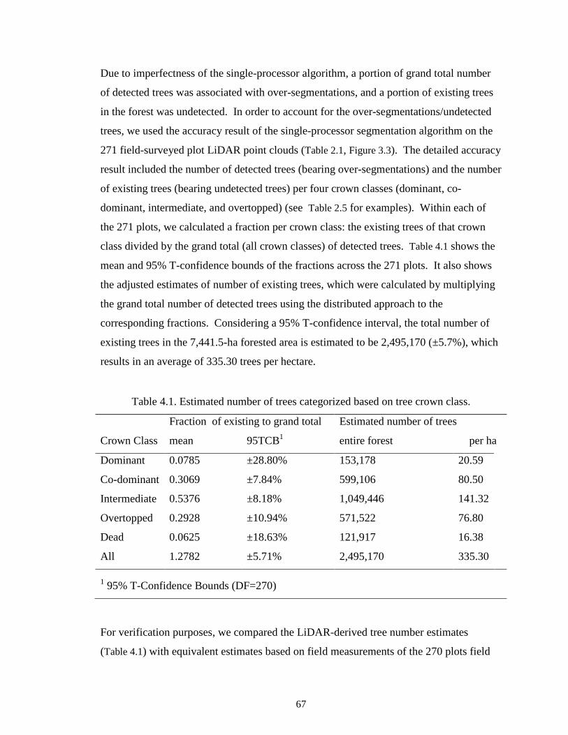
67
Due to imperfectness of the single-processor algorithm, a portion of grand total number
of detected trees was associated with over-segmentations, and a portion of existing trees
in the forest was undetected. In order to account for the over-segmentations/undetected
trees, we used the accuracy result of the single-processor segmentation algorithm on the
271 field-surveyed plot LiDAR point clouds (Table 2.1, Figure 3.3). The detailed accuracy
result included the number of detected trees (bearing over-segmentations) and the number
of existing trees (bearing undetected trees) per four crown classes (dominant, co-
dominant, intermediate, and overtopped) (see Table 2.5 for examples). Within each of
the 271 plots, we calculated a fraction per crown class: the existing trees of that crown
class divided by the grand total (all crown classes) of detected trees. Table 4.1 shows the
mean and 95% T-confidence bounds of the fractions across the 271 plots. It also shows
the adjusted estimates of number of existing trees, which were calculated by multiplying
the grand total number of detected trees using the distributed approach to the
corresponding fractions. Considering a 95% T-confidence interval, the total number of
existing trees in the 7,441.5-ha forested area is estimated to be 2,495,170 (±5.7%), which
results in an average of 335.30 trees per hectare.
Table 4.1. Estimated number of trees categorized based on tree crown class.
Fraction of existing to grand total Estimated number of trees
Crown Class mean 95TCB1 entire forest per ha
Dominant 0.0785 ±28.80% 153,178 20.59
Co-dominant 0.3069 ±7.84% 599,106 80.50
Intermediate 0.5376 ±8.18% 1,049,446 141.32
Overtopped 0.2928 ±10.94% 571,522 76.80
Dead 0.0625 ±18.63% 121,917 16.38
All 1.2782 ±5.71% 2,495,170 335.30
1 95% T-Confidence Bounds (DF=270)
For verification purposes, we compared the LiDAR-derived tree number estimates
(Table 4.1) with equivalent estimates based on field measurements of the 270 plots field

68
surveyed in Robinson Forest (Table 2.1). The estimates for total number of trees per ha
differ by about 3% (~342 LiDAR-derived compared with ~326 field estimated) and the
estimates of number of dominant trees per ha differ by about 30% (~21 LiDAR-derived
compared with ~15 field estimated). However, the large overlaps between the 95%
confidence interval errors indicate no statistically significant differences.
Figure 4.8. Estimated number of trees using LiDAR compared to field-collected along
with the 95% confidence intervals.
Figure 4.9 shows the height distribution of all detected trees (heights above 5 m)
by the approach. The height distribution follows a bimodal pattern, which can be
attributed to multistory structure of deciduous natural forests, in which the dominant and
co-dominant trees form the overstory and intermediate and overtopped trees form the
understory tree canopy layers. We fitted a normal mixture model to the bimodal

69
distribution: the larger lump on the right (associated with overstory trees) has a mean
height of 26.9 m and a standard deviation of 6.6 m, and the smaller lump (associated with
understory trees) has a mean height of 9.4 m and a standard deviation of 2.6 m.
Figure 4.9. Height distribution of 1,994,970 trees detected in Robinson Forest
superimposed with an estimated normal mixture model.
We compared the LiDAR-derived mean tree height estimates with those obtained
from the 271 field surveyed plots (371 overstory and 826 understory trees). The sample
mean height of the overstory trees was 25.4 m with a standard deviation of 5.3 m, and the
sample mean height of understory trees was 17.0 m with a standard deviation of 4.1 m.
Considering that the LiDAR-detected tree heights are in fact biased by presence of falsely
detected (mostly overstory) trees and absence of undetected (mostly understory) trees, the
field estimates are close to the LiDAR-detected estimates for overstory trees. However,
the field estimates for understory trees are remarkably larger than the LiDAR-detected
estimates, which can be justified as follows. As investigated in the previous chapter,

70
airborne LiDAR provides considerably less information about the understory trees due to
decreased penetration of LiDAR points toward bottom canopy layers, hence detected tree
rate is lower for understory trees. Also, the detected understory trees are likely biased to
be smaller within the population of all existing understory trees because they are easier to
detect when there is less canopy closure, which is associated with stand age and is
minimal when stand is young and in general has smaller trees [81]. So, detecting
relatively fewer mid-story trees that are also likely biased to be smaller leads to capturing
a distribution with smaller mean and standard deviation. After all, the only information
used to fit the normal mixture model was the heights of the trees while height may not be
sufficient for classification, i.e., a moderately tall tree can in fact be mid-story if situated
in a taller stand while the mixture model always probabilizes it strongly as over-story
according to its height, and vice versa. Thus, the procedure of fitting the normal mixture
model likely separates the two tree classes more distantly with respect to height.
4.4 Conclusion
Obtaining tree-level information over large forested areas is increasingly
important for accurate assessment, monitoring and management of forests and natural
resources. Several automated tree segmentation methods have been developed, but these
methods have only been applied to small forested areas for accuracy assessment.
Although these methods can in theory be applied to larger areas, such applications is not
straightforward because LiDAR data covering forest-level data far exceeds the memory
of desktop computers and may also take unacceptably long time to be processed
sequentially. Here we presented and analyzed a scalable distributed approach that was
applied to segment trees within a LiDAR point cloud covering an entire forest. The
distributed approach segmented trees within the tiles and across the tile boundaries, and
introduced a minimal bias compared with the single-processor algorithm that was also
quantified in this work. Comparison of the estimated number of trees and the tree height
distribution with the field surveys validated sound operation of the approach. We
presented the distributed processing approach and the associated analysis in a platform-
independent manner so as the implementation can be accomplished on different
distributed platforms with minor modifications. Although the distributed approach was

71
presented within the context of tree segmentation from LiDAR point clouds, it can
straightforwardly be applied to segment/identify objects within other large-scale datasets.
In addition to providing number of trees and height distributions (compared here
to field surveys for validation), the distributed approach enables identification of
individual tree locations and attributes (tree height and crown widths) as well as the point
cloud segments representing tree crowns for large forested areas in a timely manner,
which in turn enables building a detailed (at the individual tree level) forest model and
performing a myriad of more accurate analyses. For instance, tree attributes can be used
to develop allometric equations to estimate other important tree metrics such as DBH and
volume, and the point cloud segments can be used to construct the 3D geometric shape of
each individual tree crown to develop mode detail estimates such as crown volume,
biomass, and carbon content. Moreover, point cloud segments representing individual
tree crowns can be used to predict non-allometric attributes such as species, type, and age
using machine learning methods, which is the subject of the next chapter. The resulting
detailed, tree-level information has the potential to increase the accuracy of forest level
information by creating remotely sensed forest inventories for more efficient
management of forest and natural resources.

72
4.A Implementation of segmentation algorithm and runtime analysis
The tree segmentation algorithm presented in Chapter 2, which was used as a building
block for evaluation in Section 4.3.1, consisted of a pre-processing step including
homogenizing the point cloud, removing non-surface points, smoothing, and then a loop
over the five major steps outlined below until the entire point cloud is clustered: 1) locate
the non-clustered highest point - global maximum (GMX); 2) generate vertical profiles
originating from the GMX with a length of maximum tree crown radius; 3) For each
profile, identify the LiDAR point along the profile that represents the crown boundary; 4)
create a convex hull of the identified boundary points; and 5) cluster all LiDAR points
encompassed within the convex hull as the highest tree crown.
For an efficient implementation of the segmentation method, the point cloud
should be indexed in a 2D horizontal grid. Indexing and the pre-processing step takes
O(n) where n is the number of points. We assume that the main loop iterates m times.
Naively locating the GMX (step 1) takes O(n) per iteration. Instead, we create a
descendingly sorted list of all of the grid cells according to the height of the point they
contain and mark all cells as unvisited. The sorting procedure takes O(n.㏒n). The grid
cells are marked as visited when they are clustered in step 5. To locate the non-clustered
GMX, the sorted list is traversed from the position of the previous GMX forward, which
on average takes O(n/m) per iteration. Once the GMX is located, clustering the highest
tree (steps 2–5) has a runtime independent of n and m and is proportional to the tree size,
which is bounded and can be assumed as a constant. So, the aggregate runtime of each
iteration of the loop is O(m/n), hence the total runtime of the loop becomes O(n).
Aggregating the pre-processing and the sorting times:
( ) ( ) ( .log )sT n O n O n n= + 4.6

73
where Ts(n) is the total runtime of the algorithm; the first term on the right-hand side
corresponds to the runtime of the main loop and the pre-processing step; and the second
term corresponds to the runtime of the sorting procedure before the loop.
We ran the implementation above on a workstation of 3.4 GHz CPU speed and 8
GB of RAM for 25 loads of data. Figure 4.10 shows the log-log plot of the runtime of the
segmentation versus the number of points.
Figure 4.10. Log-log plot of the Segmentation runtime versus the number of LiDAR
points in the point cloud. Each symbol corresponds to average across 15 strata.
The slope of the best fit line to the square symbols is 1.03, which concurs with the linear
term of Equation 4.6. Also, the slope of the best fit line to the triangle symbols is 1.23
showing a slightly super-linear pattern, which concurs with the non-linear term in the

74
equation. We measured the constant coefficients of both terms by dividing the execution
times associated with the terms by n and n.㏒n respectively. The ratio of the linear
coefficient to the non-linear one is platform-independent and is about 7,800 according to
our measurement. This yields that n should be greater than 27,800 in order for the non-
linear term to start dominating the linear term, which corresponds to a LiDAR point
cloud covering over 3e+2,331 times surface area of the earth. So, we may safely replace
㏒n in the non-linear term with an upper bound constant, which reduces Equation 4.6 to:
( ) ( )sT n O n= 4.7
Copyright © Hamid Hamraz 2018

75
5 Deep Learning for Predicting Tree Type
Segmented LiDAR point clouds representing individual tree crowns can be used to derive
tree allometric dimensions such as height and crown width, and to predict different tree
attributes such as type (coniferous or deciduous), species, status (live or dead), or DBH
[140-142]. Several studies have used machine learning methods to predict tree type or
species [31-33, 96, 143-146]. In these studies, researchers derived a set of features
related to crown geometry and foliage density/pattern/texture from the LiDAR data and
input the features into different classification methods such as linear discriminant
analysis, k-nearest neighbors, random forest, and support vector machines (SVMs). A
few studies have presented automated or semi-automated approaches for identifying
useful features for the task of tree species classification [147-149]. The previous work
using traditional learning methods has required that the set of candidate features be
assembled by an expert, with the intention of removing redundant and less useful
information from the raw data. However, because LiDAR point clouds are not easily
processed by the human visual system, the expert-designed features may as well be
suboptimal and likely missing useful information.
Deep neural network learning methods, on the other hand, can directly map the input raw
data to the target prediction by passing the input through multiple layers [150, 151]. The
initial layers are designed to extract the useful low to high level features, and the next
layers map the extracted features to the target prediction. The advantage of deep learning
methods is in their end-to-end operation, i.e., both feature extraction and mapping to the
target prediction are trained automatically as a whole such that the global prediction task
functions optimally. Although some expertise is required to set up a reasonable deep
network architecture and tune the optimization hyper-parameters, no human intervention
is required for feature extraction. In this chapter, we discretize segmented point clouds
representing tree crowns in order to input them into a deep convolutional neural network
(CNN) architecture, and perform different deep learning experiments on tree type
classification [152]. We review the related literature in Section 5.1. In Section 5.2, we
describe the data preparation steps, i.e., normalization of LiDAR intensity values,
registration of segmented point clouds to field data to create a training dataset, and two
discrete representations for a crown cloud so as to enable its input to a CNN. Section 5.3

76
is devoted to the description of the CNN architectures to run our deep learning
experiments, an iterative resampling method to correct potential mislabels in our training
data, and the road maps of our experiments. In Section 5.4, we present results and
discussions where we thoroughly investigate the effects of different design decisions with
respect to training data preparation and deep network structure as well as the effects of
training data composition and domain-specific data on the classification accuracy.
Finally, Section 5.5 concludes the chapter.
5.1 Literature review
A large body of research has been devoted to a variety of deep learning classification or
segmentation tasks using 2D images as the raw input data [153-159]. However, 3D data
have attracted less attention due to more costly acquisition/processing and their less
intuitive and less conventional representational formats, which demand non-trivial pre-
processing techniques to discretize the data and make them usable for deep learning
methods [160, 161]. A number of studies have binned 3D data into voxel spaces to create
representations that can be input to and processed by a 3D convolutional neural network
(CNN) [162-164]. Although voxel spaces are perhaps the most comprehensive discrete
representations that preserve the raw 3D structure, they are computationally expensive to
process, more prone to overfitting, and therefore prohibitive for use with larger datasets.
Other studies have created 2.5D digital surface models (DSMs) [165-167] or multiple 2D
views [168, 169] from the 3D data. In the event that 3D imaging/sensing technology can
capture the internal structure of the measured objects, conversion to DSM or 2D views
may forego this internal structure. However, depending on the application, DSMs and/or
multiple 2D views can provide as much useful information as a full 3D representation
while being less prone to overfitting and incurring less computational cost [168, 170].
A few recent studies used deep learning methods to classify species of individual trees
from very high resolution ground-based LiDAR point clouds. Guan et al. [171]
segmented individual trees from mobile LiDAR point clouds in an urban area, developed
a waveform representation to model the geometry of the trees, and used deep learning to
convert the waveform representation to high-level features. These features were then
input to an SVM classifier to perform tree species classification. Mizoguchi et al. [167]
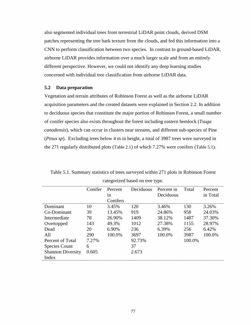
77
also segmented individual trees from terrestrial LiDAR point clouds, derived DSM
patches representing the tree bark texture from the clouds, and fed this information into a
CNN to perform classification between two species. In contrast to ground-based LiDAR,
airborne LiDAR provides information over a much larger scale and from an entirely
different perspective. However, we could not identify any deep learning studies
concerned with individual tree classification from airborne LiDAR data.
5.2 Data preparation
Vegetation and terrain attributes of Robinson Forest as well as the airborne LiDAR
acquisition parameters and the created datasets were explained in Section 2.2. In addition
to deciduous species that constitute the major portion of Robinson Forest, a small number
of conifer species also exists throughout the forest including eastern hemlock (Tsuga
canadensis), which can occur in clusters near streams, and different sub-species of Pine
(Pinus sp). Excluding trees below 4 m in height, a total of 3987 trees were surveyed in
the 271 regularly distributed plots (Table 2.1) of which 7.27% were conifers (Table 5.1).
Table 5.1. Summary statistics of trees surveyed within 271 plots in Robinson Forest
categorized based on tree type.
Conifer Percent in Conifers
Deciduous Percent in Deciduous
Total Percent in Total
Dominant 10 3.45% 120 3.46% 130 3.26% Co-Dominant 39 13.45% 919 24.86% 958 24.03% Intermediate 78 26.90% 1409 38.12% 1487 37.30% Overtopped 143 49.3% 1012 27.38% 1155 28.97% Dead 20 6.90% 236 6.39% 256 6.42% All 290 100.0% 3697 100.0% 3987 100.0% Percent of Total 7.27% 92.73% 100.0% Species Count 6 37 Shannon Diversity Index
0.605 2.673

78
5.2.1 Intensity normalization
The LiDAR intensity value that is recorded for each return is dependent on various
factors, many of which are unrelated to the vegetation texture [172, 173]. The distance a
LiDAR pulse travels (referred to as range), the angle at which the pulse is emitted, and
the LiDAR return number are among the factors affecting intensity that can be controlled
for, while different atmospheric factors are difficult to track. Assuming constant
atmospheric conditions, we used a data-driven approach to normalize the intensity values.
We binned the entire forest dataset to a horizontal grid with a cell width of 10 m and
randomly sampled one leaf-off and one leaf-on vegetation point per grid cell. We then
grouped the leaf-off and the leaf-on samples according to the return number to create
three leaf-off and four leaf-on datasets. For each of the seven datasets, we built a
regression model that predicted intensity based on range and emission angle. For the
leaf-on datasets, the effect of range and angle was significant: the natural logarithm of
range had a negative correlation with intensity (P < .0001), and the cosine of angle has a
positive correlation (P < .0001) with intensity. However, we did not observe any
significant correlations between range/angle and intensity for the leaf-off datasets, which
is likely due to the recording of very low intensity values and discretization to an eight-
bit format, dimming away such correlations. For each of the four leaf-on datasets, we
removed the effects of range and emission angle by residualization [174], i.e., we
replaced the intensity values by the corresponding model residuals. Finally, we
normalized the residualized intensities back to an eight-bit format.
5.2.2 Registration with field data
We used the segmented point clouds of the 271 field surveyed plots of Robinson Forest,
which were created by the multi-story segmentation method described in Chapters 2
and 3,. Similar to the evaluation procedure described in Section 2.4.2, in order to register
the segmented crowns with the field data, we assigned a score to each pair of segmented
crown and field-measured stem locations.
The location of each segmented crown was taken from the crown apex. Scores were
assigned based on the difference in tree height and the leaning angle from nadir between
the crown apex and the stem location. If the height difference was less than 10% and the

79
leaning angle was less than 5°, a score of 100 was assigned. If the height difference and
leaning angle were less than 20% and 10° respectively, a score of 70 was assigned. If the
height difference and leaning angle were less than 30% and 15°, a score of 40 was
assigned. Otherwise, a score of 0 was assigned. We then selected the set of pairs with
the maximum total score where each crown or stem location appears not more than once
using the Hungarian assignment algorithm and regarded the set as the co-registered tree
pairs [70]. Excluding dead trees, a total of 2528 co-registered trees was gleaned, of
which 124 (4.90%) were conifers and 2404 (95.10%) were deciduous. Smaller
understory trees, especially those represented by very low point densities, were
automatically excluded through the segmentation and registration process.
5.2.3 Discretization of crown point clouds and data augmentation
We converted the point cloud of each tree crown to two different representational
formats: (1) a DSM with four channels (DSM×4), and (2) a set of four single-channel 2D
images (4×2D). To create the DSM×4 format, we binned the point cloud to a horizontal
grid of 128×128 pixels of width 12.5 cm such that the apex of the segmented crown
would fall in the center pixel. We then recorded the four channel values for each pixel,
which included the elevation above ground of the highest leaf-on point, the normalized
intensity of the highest leaf-on point, the elevation above ground of the highest leaf-off
point, and the intensity for the highest leaf-off point. We chose the small pixel width of
12.5 cm for creating the DSM image to minimize the information loss because of falling
multiple LiDAR points in a pixel. The resulting DSM structure captures a square of
16×16 m in the real world, which is large enough to encompass an entire tree crown in
almost all cases given that tree crowns are often very tightly situated in dense forests.
However, because crown width information may be missing for some large trees, we
recorded the crown area as a separate feature alongside the DSM×4 representation.
To create the 4×2D format, we generated one pair of aerial view images and one pair of
side profile view images for each segmented crown. One image in each pair was created
from the leaf-on point cloud, and the other was created from the leaf-off point cloud. As
with the DSM×4 format, the aerial images for a single tree crown covered a square area
of 16×16 m, with the crown apex located in the center of the images. The pixel width

80
however, was set to 25 cm because depth information was not intended to be captured in
the aerial view. To create the aerial images, we recorded the intensity of the highest
LiDAR point in each pixel. The side profile images were created from vertical profiles of
the point clouds, which had a thickness of 75 cm and passed through the crown apex.
Each of the side view images captured a square area of 16×16 m with a pixel width of 25
cm. The LiDAR point representing the apex was located in the top center pixel. We
recorded the mean intensity of leaf-on/leaf-off LiDAR points in the profile for each pixel.
Although the majority of trees in our dataset are taller than 16 m, most airborne LiDAR
points are recorded in the upper parts of the tree crowns and therefore, a 16 m side view
height was deemed sufficient to capture the crown structure that is represented by the
LiDAR points. However, because tree height information was missing from both the
aerial and side views, we recorded height and crown width as two separate features
alongside the 4x2D representation.
The DSM×4 format resembles the 3D point cloud data by losing less 3D structure while
the 4×2D format only captures the 3D data from two 2D views taking the advantage of
the symmetry of an ideally shaped tree crown. To augment the data and increase the
training data size for deep learning experiments, we created the DSM×4 and the 4×2D
representational formats over 180 rotational variations of each point cloud. We
iteratively rotated the point cloud along a nadir axis through the apex by 2° and created a
DSM× 4and a 4×2D representation in each iteration. Although the 4×2D format loses
much of the 3D information because in reality the tree crowns has several dissymmetrical
structural features, this information has mostly been re-gained when using 180 rotational
augmentations per instance.
5.3 Deep learning
5.3.1 Convolutional neural network models
For the DSM×4 input format, we stacked six pairs of convolutional and max pooling
layers including ReLU activation units. Each convolutional layer included one filter of
4×3×3 with a stride of one pixel that was operating on a zero-padded input to maintain
the same size for the output. Each max pooling layer included 2×2 max pooling windows
per channel, down-sampling the convoluted input to half of the width and the height.

81
Operating on the representation input of size 4×128×128, this layer composition produces
a 4×2×2 output structure, which is flattened to 16 output units. On the other hand, for the
crown area input feature, we stacked two dense layers, each including two ReLU units.
We then put the 16 units initiated from the DSM image and the two units initiated from
the crown area feature together and stacked two dense layers of 25 and 10 ReLU units
respectively to the end. Finally, we added a softmax layer to obtain the probability
distribution over one-hot-encoded class labels.
For the 4×2D input format, we stacked five pairs of convolutional and max pooling
layers, including ReLU activation units, per each single-channel 2D image. Each
convolutional layer included one filter of size 1×3×3×1 with a stride of one pixel that was
operating on a zero-padded input. Each max pooling layer included windows of 2×2,
down-sampling the convoluted input image to half of the width and the height. Operating
on the set of four image representation inputs of size 1×64×64, this layer composition
produces a 2×2×4 output structure, which is flattened to 16 output units. On the other
hand, for the crown width and the tree height input features, we stacked two dense layers,
including four and two ReLU units respectively. Similar to the DSM network, we put the
previous 18 units together and added two dense layers of 25 and 10 ReLU units and a
final softmax layer respectively to the end.
The DSM×4 format allows the deep network architecture to perform an early fusion of
the leaf-on and leaf-off data as well as the intensity and height values associated with the
data. The network captures the correlation between the four channels for the
classification task by including more parameters and intermediate features. On the other
hand, the 4×2D format allows a late fusion to the network, i.e., the leaf-off and leaf-on
data and their intensity/height values are not fused until after the corresponding
convolutional and max pooling layers produced features independently. While the
DSM×4 format allows for a richer training model, the 4×2D format incurs less
computational cost.
5.3.2 Mislabel correction via iterative resampling
As described earlier, registration of the segmented tree crowns to the field-surveyed tree
stem locations was done through a probabilistic scoring process. Moreover, the GPS

82
error for the field-surveyed plot centers (~5 m) can exceed the distances between
individual trees. These issues likely resulted in a fraction of mis-registrations hence
yielding mislabels for the classification task in this work. Mislabeling occurs when a
field-surveyed coniferous tree stem is assigned to a segmented deciduous tree crown or
vice versa. In the semi-supervised learning literature, a number of studies trained
learning models that are robust to such noise by modifying the learning model to
explicitly account for the noise [175-177], although these studies did not necessarily
correct mislabels for external use. Other studies attempted to eliminate/correct mislabels
by training learning models and identified mislabels by performing statistical inference
on the classification result of the trained models [178, 179]. These studies either used a
small noise-free dataset or, when that was not possible, made assumptions about the
tolerable amount of noise in their data to train their learning models for identifying
mislabels. For the latter scenario, some studies reported successful identification of
mislabels in the presence of up to 40% noise in the training data [179]. Unlike general
RGB images that are specifically designed for human visual comprehension, remotely
sensed LiDAR-represented tree crowns are difficult and uncertain for human experts to
classify, making it infeasible to create a noise-free dataset to start with. Therefore, we
performed mislabel correction through ensemble filtering [180], which is derived by a
series of resampling and statistical inferences.
We built 100 4×2D-input networks, and each network was trained using a random sample
of 80 deciduous and 80 conifer instances from our labeled dataset. Random sampling
was performed without replacement: once all corresponding labeled instances were used,
we started over and continued until all 100 networks were built. This randomization
pattern ensured that all instances of a class had (almost) equal contributions across all of
the networks in the training process. To train the networks, we used the Keras deep
learning library: we set the loss function to categorical cross entropy and ran the Adam
optimizer (learning rate = 0.01) [181]. The training of each network was performed for
three epochs in order to ensure that the process converged to a reasonable state, i.e., the
training accuracy was lifted from the base accuracy of 50% but did not reach an
overfitting phase.

83
For each network n, we computed the average of the test accuracies of n over the 180
augmented forms (accni) for every instance i in the labeled dataset if i was not used in
training n. Assuming instance i is correctly labeled, its test accuracy should on average
be equal to the training accuracy of the trained network n (accn). On the other hand,
when instance i is mislabeled, its test accuracy should on average be equal to the
symmetric value of the training accuracy of n about the base accuracy of 50% (1 - accn).
Therefore, if accni is less than the symmetric value of the training accuracy of n about
50%, i.e., accni < 1 - accn, it is very likely that i is mislabeled. Using all 100 networks,
we generated values of accni - (1-accn) per each instance i and used these values to
perform a T-test on whether their mean was less than zero. If the T-test indicated that an
instance was mislabeled, we flipped the label for that instance. We repeated the process
of training 100 networks, performing T-tests, and flipping mislabels until no mislabels
were identified. Since 2,528 T-tests were performed in each iteration, we used the
significance level of 10-8 for the T-tests. This significance level, according to the
conservative Bonferroni principle, would not allow a false positive rate of more than
0.0025% per iteration.
5.3.3 Classification and evaluation
After correcting potential mislabels, we used an ensemble of 50 networks to perform the
classification. We trained each network on a random sample of 100 deciduous and 100
coniferous instances using the Adam optimizer with a learning rate of 0.01. Random
sampling was performed without replacement as mentioned above. The ensemble
training scheme was used to minimize the bias of unbalanced training instances in each
class, i.e., to train each network on a balanced sample while taking advantage of the
entire dataset. To perform the classification for a given instance, we averaged over the
softmax probabilities produced by all of networks that did not use that instance for
training and assigned the class as that with the larger average probability. This training
and testing pattern allowed us to produce cross validated classification accuracies for all
of the instances in our dataset. We performed the same ensemble procedure for both the
DSM×4 and the 4×2D formats. The training was run for fifteen epochs for every DSM×4
input network, but five epochs appeared to be sufficient for every 4×2D input network.

84
For the rest of experiments, we used the 4×2D format because of the lower computational
load.
To investigate the effect of the training data size, we created stratified random
subsamples of our dataset. We subsampled 20%, 40%, ..., 100% of the deciduous and
coniferous trees and performed the cross validated classification procedure described
above for each subsampled dataset. We adjusted the size of resampling instances in
proportion to the subsample size, though the number of ensemble networks was held
constant. To quantify the effect of data augmentation, we measured the cross validation
accuracies for when 20, 40, ..., 180, 240, 300, and 360 rotations of each instance were
included. We then looked into the effects of the domain parameters: we ran the cross
validation experiment excluding leaf-off data, excluding leaf-on data, using non-
normalized intensities for leaf-on data, and excluding intensity values (using binary
values representing existence of a point per pixel). When excluding leaf-on and leaf-off
data, we decreased the size of the last two dense layers before the softmax layer to 16 and
8 units respectively to account for the smaller input size. We also inspected the
correlation between the point density of a crown cloud and the probability of the softmax
output unit associated with the correct label of the crown cloud to determine how point
density affected the classification accuracy. Lastly, we stratified the classification result
to overstory (dominant and co-dominant) and understory (intermediate and overtopped)
trees to inspect how crown class affected the classification performance.
5.4 Results and discussions
5.4.1 Mislabel correction
The process of mislabel correction converged after 13 iterations and increased the
number of conifers from 124 to 214 and decreased the number of deciduous trees from
2404 to 2314 (Figure 5.1). According to the original field measurements (Table 5.1),
7.27% of the trees in RF are conifers, which is slightly lower than the result after
correcting mislabels – 8.46% conifers. The reason for this slight difference may be the
relative difficulty in segmenting deciduous trees compared to coniferous trees due to the
variety of crown shapes and the looser, interwoven foliage, which creates complicated,
difficult-to-distinguish LiDAR point patterns [88]. This effect likely resulted in larger

85
rate of undetected deciduous trees after segmentation and registration with the field data.
In total, the labels for 35 of the initial 124 (28.22%) conifers and 125 of 2404 (5.20%)
initial deciduous trees were flipped. These unbalanced flip rates concur with the
dominant presence of deciduous trees, i.e., if a field deciduous tree is mis-registered to a
LiDAR crown, the crown is likely another deciduous tree (yielding no mislabel) while for
a mis-registered field conifer this is not the case. Over the 13 iterations of the mislabel
correction procedure, the average training accuracy of the 100 networks started at 67.1%
and plateaued at 83.6% (Figure 5.2). This trend suggests that a number of highly likely
(controlled by the T-tests) mislabels were corrected, improving the model accuracy,
while less likely mislabels were left unchanged, resulting in the accuracy plateau and
prohibition of overfitting. Overall, the mislabel correction process produced more
realistic labels by increasing the number of coniferous trees from 4.90% to 8.46% within
the 2528 segmented tree crowns.
Figure 5.1. Rates of flip for coniferous and deciduous instances over the 13 iterations of
the mislable correction process.

86
Figure 5.2. Average training accuracy of 100 networks over the 13 iterations of the
mislabel correction process.
5.4.2 Classification accuracy
The cross-validated accuracies associated with the DSM×4 representation were
80.4±5.3% for conifers and 90.1±1.3% for deciduous trees at a confidence level of 95%.
The equivalent classification accuracies associated with the 4×2D representation were
82.7±5.1% and 90.2±1.3%, respectively for coniferous and deciduous trees (Figure 5.3).
Higher accuracy values associated with the 4x2D representation were insignificant and
are likely due to the fact that this format was used for the mislabel correction process,
which might have slightly biased the data. As mentioned, the DSM×4 format more
closely resembles 3D data, which together with the richer early-fused network, have the
potential to achieve higher classification accuracies. However, the 4×2D format with a
late-fused network could achieve similar accuracies while incurring less computational
load.

87
Figure 5.3. Classification accuracy when using the two representational formats derived
from discretization of LiDAR point clouds.
5.4.3 Effect of training data size
Increasing the size of training data improved the classification accuracies. For deciduous
trees the accuracy plateaued when using only 40% of the original dataset (~925
deciduous and ~86 coniferous trees) but for coniferous trees, the accuracy appeared to be
increasing with even more number of conifer instances than the original 214 ones
(Figure 5.4). This observation suggests that a balanced dataset of close to one thousand
instances per class would likely have been an optimal dataset for this classification task
and could have brought the accuracy of coniferous trees closer to that of deciduous trees.

88
Figure 5.4. Classification accuracies measured against the size of the training data. Each
symbol in the diagram represents the average of 20 observations.
5.4.4 Effect of data augmentation
Including a greater number of rotational augmentations per instance slightly improved the
classification accuracies. Using only 20 rotations per instance resulted in 73.8% accuracy
for coniferous trees and 87.7% accuracy for deciduous trees, which are lower than when
using the original 180 rotations. The improvement in classification plateaued at ~60
rotations for deciduous trees and ~150 rotations for coniferous trees (Figure 5.5). Having
more deciduous trees likely resulted in a smaller number of rotations/augmentations to be
sufficient for the classification task. Although a higher number of rotations could
compensate for the small number of coniferous training instances to some extent,
augmentations are unlikely to match the classification quality provided by a higher
number of real training instances.

89
Figure 5.5. Classification accuracies measured against the number of rotational
augmentations per instance.
5.4.5 Effect of domain data
Excluding the leaf-off data resulted in a remarkable decrease in classification accuracy
for the conifers (from 82.7% to 61.2%) and a minor decrease in accuracy for deciduous
trees (from 90.5% to 89.6%), while excluding the leaf-on data resulted in a minor
decrease in accuracy for conifers (from 82.7% to 81.6%) and a negligible increase in
accuracy for deciduous trees (from 90.5% to 90.7%) (Figure 5). This observation
indicates that, despite the much lower point density, the leaf-off data provided the most
useful features for the classification task, which concurs with the result of the previous
work [33, 143]. As conifers do not lose their dense foliage during the winter, the leaf-off
LiDAR points could represent their crown shapes even at a low density while the
deciduous trees may only be represented by a few random LiDAR points returning from
their defoliated branches. The dense leaf-on data could on the other hand represent the
crown shapes for both conifers and deciduous trees and was used here for segmentation
of the individual tree crowns. Attempting to distinguish the crown shapes of deciduous
and coniferous trees using leaf-on data is likely less efficient than distinguishing between
a random point pattern (a deciduous tree) and a crown-like shape (a coniferous tree) using

90
the leaf-off data. However, for identifying species, which is a more complicated
classification task and a subject of future work, the high density leaf-on data may be more
useful.
Using binary values instead of the intensity values resulted in a remarkable decrease in
classification accuracy for conifers (from 82.7% to 69.2%) and only a negligible increase
in accuracy for deciduous trees (from 91.5% to 92.1%) (Figure 5.6). Using the
normalized intensity values for the leaf-on data (when excluding the leaf-off data)
compared with using non-normalized values, seemed to make minor, insignificant
improvements in the classification accuracies for conifers (from 60.3% to 61.2%) and
deciduous trees (from 88.9% to 89.6%) (Figure 5.6). Although LiDAR intensity values
were useful for the classification, the uncontrollable atmospheric factors present during
LiDAR acquisition and the discretization to an eight-bit format likely introduced some
level of noise, yielding the process of intensity normalization less effective than expected.
Lastly, some domain data, i.e., the leaf-off data and the intensity values, appeared to be
very important in the classification task, which is evident in the remarkable changes in
the accuracy for conifers (Figure 5.6). However, as observed by only slight changes in
the accuracy of deciduous trees, abundance of training data likely compensates for the
absence of a subset of important domain data.

Figure 5.6. Classification accuracies when excluding domain data.
91

92
5.4.6 Effects of crown class and point density
For overstory trees, the cross validated classification accuracy was 92.1±4.7% for
conifers and 87.2±2.2% for deciduous trees. The classification accuracy for understory
trees was 69.0±9.8% for conifers and 92.1±1.4% for deciduous trees (Figure 5.7). The
crown of an understory tree is typically captured only partially by airborne LiDAR, as it
is covered by the overstory trees. The partial shapes of these crowns decrease the
classification power, likely yielding the correlated accuracies to become easily biased by
the abundance of deciduous instances compared with coniferous instances. In contrast,
the crowns of overstory trees are captured more completely allowing for a more powerful
classification process. Lastly, we could not identify any significant correlation between
point density (neither leaf-off nor leaf-on) and the classification accuracy (neither for
overstory nor for understory trees). This observation does not concur with previous work
reporting a positive correlation between accuracy and point density [149]. The reason is
likely that the classification task is primarily driven by the leaf-off data, the point density
range of which is too small (0.1-6.0 pt/m² for the middle 95%) to surface any effect.
Moreover, the partial crowns captured may feature high point densities but are not easy to
classify due to their incomplete shapes.

93
Figure 5.7. Classification accuracy of overstory and understory trees.
5.5 Conclusions
Airborne LiDAR point clouds representing individual trees can be used to predict tree
attributes such as tree type. Previous work exploited shallow learning techniques that
require the engineering of useful features by a human expert. In this work, we used deep
learning CNNs to classify crown point clouds as coniferous or deciduous trees. We
segmented individual trees from the LiDAR point clouds and registered them with field-
surveyed trees to create training data. We designed two different discrete representations
of a crown’s 3D point cloud and the corresponding deep learning architectures. We used
ensemble learning schemes including several networks trained on balanced subsamples of
training data to perform mislabel correction (driven by statistical tests) and to measure
the cross-validated classification accuracies in different scenarios.
Our investigation of the coniferous/deciduous deep learning classification showed that a
set of 2D views/profiles of a 3D point cloud are not only more efficient to be processed
but also can yield similar or even higher accuracies compared with bulkier 2.5D (or even

94
3D) representations. Moreover, late fusion of features in a CNN architecture may
provide equivalent performance as compared with an early-fused architecture while
incurring less computational load. Although data augmentation can help improve the
classification accuracy, a higher number of real training instances can provide much
stronger improvements. As we observed, leaf-off LiDAR data, despite its much lower
point density in comparison with the leaf-on data, was the main source of useful
information, which is likely associated with the perennial nature of conifer foliage.
LiDAR intensity values also proved to be useful for the classification, although we could
not obtain a significant improvement by normalizing the intensity values. A large
number of training instances may compensate for the lack of a subset of important
domain data. Lastly, we observed much higher and balanced classification accuracies for
overstory trees (~90%) as compared with understory trees (~90% for deciduous and
~65% for coniferous), which is likely associated with capturing only partial shapes of
many understory tree crowns using airborne LiDAR.
The results presented indicate that deep learning can effectively and efficiently be used
for classifying tree type based on airborne LiDAR point clouds representing individual
tree crowns, which is a step forward to operational tree-level remote quantification of
large-scale forests. Although further experiments using richer datasets and for more
complicated prediction tasks (e.g., species classification) are required, deep learning
provides the feasibility of automatic extraction of optimal features toward the prediction
task. This unique deep learning characteristic brings about the potentials for successful
prediction tasks in different domains such as remote sensing and biomedical image
analysis, where the data modalities are not friendly to the human perceptual system and
have likely operated using suboptimal human-designed features.
Copyright © Hamid Hamraz 2018

95
6 Conclusions and Future Directions
Airborne LiDAR technology can record point clouds representing 3D forest canopy
structure and the terrain underneath over large geographical regions in a relatively short
time. The LiDAR point clouds can be processed to identify individual trees both from
overstory and understory canopy layers and derive their horizontal and vertical
structures/distributions. This detailed tree-level information is not only quicker and less
costly to acquire but increases the accuracy of various estimates consumed in forest and
natural resources management. In this dissertation research, we developed automated
methods for processing LiDAR point clouds in order to model a forest at the individual
tree level. In Section 6.1, we present a summary of major contributions of this work from
the technical perspective. We then present a summary of the major results in Section 6.2.
Section 6.3 is devoted to potential spots for improvements of this work and the directions
that can be followed upon in future. Finally, in Section 6.4, we point out the implications
of these contributions for forest and natural resources management as well as similar
domains dealing with spatial data.
6.1 Summary of technical contributions
We developed a tree segmentation method (Chapter 2) that makes no prior assumptions
about tree crown shapes and sizes. The method segments the tallest tree within a given
area, removes it from the point cloud, and iterates until the point cloud is emptied. To
segment the tallest tree, the global maximum is identified as the tree apex. Then, crown
boundaries surrounding the apex are identified by inspecting vertical profiles of the point
cloud passing through the apex. Within each profile, the method first removes between
crown gaps using an outlier detection routine, and then collects crown steepness and tree
height on-the-fly and uses them to identify the crown boundary. Finally, all points
encompassed within the convex hull of the crown boundaries are clustered as the tallest
tree. Among the clustered trees, those with crown width of less than 1.5 m are removed
as noise segments. The major novelty of this method is that it does not make prior
assumptions about tree shape and size, hence it can readily be applied to different forest
types.

96
We also developed a vertical stratification method (Chapter 3) that decomposes the point
cloud to an overstory and multiple understory tree canopy layers. The stratification
method removes the top canopy layer by inspecting vertical distributions of LiDAR
points within overlapping locales and continues until the point cloud is emptied. Within
each locale, the LiDAR point heights are binned to a histogram and then the two highest
salient curves of the histogram are identified as the top and the second top canopy layer.
The middle of the gap between the two top layers is regarded as the threshold to remove
the top canopy layer in the center point of the locale. Using overlapping locales to
determine the thresholds results in the top canopy layer to smoothly adjust to vertical
variability of tree crown height within an unconstrained area, which is the major novelty
of this method. In order to improve detection of understory trees, the tree segmentation
method can then independently be applied to each tree canopy layer. The combination of
the vertical stratification and the tree segmentation methods can be used to segment
individual trees within multistory forest canopies.
Using the vertical stratification method, we developed a canopy occlusion model by
inspecting the decrease of canopy layer point density with proximity to the ground
(Chapter 3). We created a large sample of stratified plot point clouds and recorded the
sequence of point density fractions of the canopy layers (from the top most to the bottom
most) for each of the plots. We then fitted a logarithmic series distribution to these
fractions. We also pinpointed the point density of a point cloud where the tree
segmentation accuracies for overstory plateau. Assuming this point density is also
required to reasonably segment trees within the lower canopy layers, we derived a
function to estimate the required density of the entire point cloud. Specifically, taking the
number of highest canopy layers for which we require to segment individual trees as the
input, the derived function estimates the required LiDAR acquisition campaign. Such a
function not only sheds light on inferior segmentation of understory trees but also can be
used to perform cost/benefit analysis when ordering LiDAR campaigns.
To tackle processing the large-scale data of an entire forest, we developed a distributed
computing approach (Chapter 4). The approach exploits a master-slave processing
paradigm and adopts a tree segmentation algorithm as a building block in order to

97
efficiently segment an arbitrarily large dataset delivered in the shape of several tiles. The
slaves perform the actual segmentation of the trees while the master maintains the global
tile map and orchestrates the slaves’ collaborative work. After segmenting a tile, the tree
crowns across the tile boundaries are categorized to eight disjoint groups: four crossing
the tile corners and four crossing the tile edges. These boundary groups are transferred to
the master, which reassigns each group for processing to a slave once it receives the other
portions of the group. The master continues the process until all of the tiles and the
boundary data are segmented. We also presented a theoretical analysis of the runtime of
the distributed computing approach. The approach enables proper handling of the tile
boundary data while efficiently managing the resources of the distributed computing
environment.
Lastly, we investigated the use of deep learning for coniferous/deciduous classification of
individual trees from airborne LiDAR data (Chapter 5). To enable efficient processing
by a deep convolutional neural network (CNN), we designed two discrete representations
using leaf-off and leaf-on LiDAR data: a digital surface model with four channels,
allowing for an early fusion of leaf-on and the leaf-off data, and a set of four 2D
views/profiles, allowing for a late fusion of the data. We generated a training dataset of
labeled tree crowns by co-registering the segmented crowns with field data. Potential
mislabels due to GPS error or tree leaning were corrected using a statistical ensemble
filtering procedure. Because the training data was heavily unbalanced (~8% conifers),
we trained an ensemble of CNNs on random balanced sub-samples of augmented data.
We compared the two representation designs with respect to the classification accuracies
and investigated the effects of training data size, data augmentation, presence of leaf-
off/on data, presence/normalization of LiDAR intensity values, tree crown class and point
density on the classification accuracies. This study provides insights on the use of deep
learning for 3D data and is one of the earliest work of its kind specially within the remote
sensing domain.
6.2 Summary of results
We applied the developed methods to the University of Kentucky Robinson Forest,
which is a natural, majorly deciduous, closed-canopy forest featuring complex terrain and
98
vegetation conditions. The tree segmentation method detected ~90% of overstory and
~47% of understory trees with false positive rates of 14% and 2% respectively.
Correlations of the segmentation accuracy scores of the method with local terrain and
stand metrics was not significant, which is likely an indication of the robustness of the
method as results are not sensitive to the differences in terrain and stand structures.
Vertical stratification of the point cloud to multiple canopy layers and applying the
segmentation method independently to each canopy layer improved the detection rate of
understory trees to ~67% at the cost of increasing their false positive rate to 12%, but it
did not affect the overall segmentation accuracy of overstory trees. As shown by
inspecting correlations of the results with forest structure, the combined segmentation
method is applicable to a variety of forest types with multiple tree canopy layers. Results
of vertical stratification of the canopy showed that the point density of understory canopy
layers were suboptimal for performing a reasonable tree segmentation, suggesting that
acquiring denser LiDAR point clouds would allow more improvements in segmenting
understory trees. According to our occlusion model, a point density of about 170 pt/m² is
needed to segment understory trees located in the third layer as accurately as overstory
trees.
Our distributed computing approach segmented about two million trees within the entire
Robinson Forest LiDAR data, which were delivered in the shape of 801 tiles that cover
an area of ~7400 hectare. Implemented using MPI and run on a cluster including 192
processing cores, the distributed approach completed segmentation of Robinson Forest in
2.5 hours, showing a speedup of about ~170. We compared the results of the theoretical
and the experimental runtime analyses across four different loads of data. Both theory
and experiment showed that given a sufficiently large dataset, the distributed approach
achieves a near linear speedup, which provides scalability to arbitrarily large datasets. A
minimal bias was introduced to the number of detected trees because of trees lying across
the tile boundaries, which was quantified and adjusted for. The estimated number of
trees categorized by crown class and the associated error margins as well as the height
distribution of the detected trees aligned well with field estimations.

99
Our deep learning experiments showed high classification accuracies (~82% coniferous
and ~90% deciduous) without the need to manually assemble the features. Both of The
designed representational formats yielded similar classification accuracies while the
multiple 2D images format incurred significantly less computational load. The data
augmentation improved the classification accuracies, but more real training instances
(especially coniferous) likely results in much stronger improvements. Leaf-off LiDAR
data were the primary source of useful information, which is likely due to the perennial
nature of coniferous foliage. LiDAR intensity values also proved to be useful, but
normalization yielded no significant improvements. As we observed, large training data
may compensate for the absence of a subset of important domain data. Lastly, the
classification accuracies of overstory trees (~90%) were more balanced than those of
understory trees (~90% deciduous and ~65% coniferous), which is likely due to the
incomplete capture of understory tree crowns via airborne LiDAR.
6.3 Potential improvements and future directions
Since the field surveyed data of Robinson Forest did not include information about tree
crown boundaries or even width of the crown, we had to evaluate the segmentation
method based on matching the crown apex and potential leaning angle. This type of
evaluation focuses on detection of the trees and does not directly inspect the crown
delineations. As a result, crown delineations may not be very accurate specially given the
operation of the convex hull on the identified boundaries that may cluster some portions
of the adjacent trees into the current crown. In order to improve crown delineations, the
segmentation method may be further developed by evaluating against information about
crown boundaries. Such information may only be acquired from field survey because
manually delineating crown boundaries within the LiDAR point clouds is typically very
difficult and produces very imperfect results.
To improve crown delineations, we may use the concave polygon created by the
identified boundaries to cluster the tallest tree. While in theory this approach seems to be
more logical than clustering with a convex hull, presence of few mis-identified
boundaries could result in big issues in crown delineations. Mis-identified crown
boundaries may occur not rarely specially for a closed canopy forest where the valleys
100
between the crowns may be completely absent. One approach to correct the mis-located
crown boundaries would be to inspect the crown radii and identify in/outliers and then
simply remove the associated crown boundaries. The convex hull or the concave
polygon clustering using the rest of the boundary points likely produces better crown
delineations. Alternatively, a deep convolutional neural network model that takes a
profile image as the input and identify the location of the crown boundary as the output
may function robustly such that the concave polygon operation yield accurate results.
Moreover, running marker controlled watershed segmentation using the tree apexes,
concave polygons, or even convex hulls of the segmented crowns as the markers on the
original DSM may help yield better final crown delineations. Performing the watershed
segmentation as a post-processing step also has the advantage of clustering the segmented
noise pieces back to an appropriate crown. These ideas for improving crown delineation
can only be tested using a dataset including field measured crown boundary information
and may be followed as a future work.
Alternative to stratification/segmentation via local geometric operations, identification of
individual tree crowns may be tackled via deep neural network learning. Several studies
used deep neural networks for classifying local regions or single pixels within the input,
which essentially generates a segmentation map of the entire input [154, 182-185]. Other
studies used neural networks including multiple convolution and pooling layers followed
by multiple unpooling and deconvolutional layers to identify the objects represented
within the input [186, 187]. While the convolutional and pooling layers derive the useful
features, the unpooling and deconvolutional layers use the features to generate a pixel-
wise classified output with the same size as the input. Training the entire network
parameters is performed through a global optimization process such that the end-to-end
operation functions optimally with respect to the provided training data. However, given
the difficulty of segmentation of tree crowns even manually by visual inspection, the
most challenging part for building deep learning models is creation of a labeled dataset
for training. One approach would be to perform field surveys including accurate
information about the crown boundaries, which is clearly too costly and labor-intensive
and may not supply sufficiently large datasets. Alternatively, we can segment individual
trees using one or more automated segmentation method and fix the visually clear

101
segmentation issues to create the training data. Such an approach will take the advantage
of both automated and manual insights, which may have quite different strengths for the
segmentation process. Either of the vertical stratification or the tree crown segmentation
or both at once may be replaced by a deeply learned neural network, though efforts
required for creation of the training data and the computational cost for training and using
the neural network should be considered in either case.
Furthermore, predicting different tree attributes, such as species, age, DBH, can be
tackled using deep learning. As mentioned, deep learning techniques automatically
derive the optimal features for the classification tasks. This characteristic provides the
opportunity for major improvement in this domain as human derived features may be
suboptimal due to unfriendliness of the remote sensing data to human vision. Moreover,
different data modalities such as RGB or spectral data can straightforwardly be included
within a deep neural network architecture, and can provide the ground for more
improvements both for segmentation of tree crowns and prediction of their attributes.
However, creating training datasets to be used for learning models within the remote
sensing domains may require close inspection of the objects in the field and is not as
easy as labeling RGB images via crowd sourcing tools. Therefore, theoretically
grounded, robust semi-supervised learning paradigms that can either correct labels or
operate in the presence of considerable deal of noise with a high confidence level will be
in great demand.
Impacting correct labeling of the data, a problem we coped with in this work has been
accurately geo-referencing plot centers under the heavy occlusion of the tree canopy. In
this situation, even the most accurate GPS units may not operate correctly due to limited
signal reception. We tried laying whitely painted plywood boards at the plot centers of
103 plots of Robinson Forest during the LiDAR acquisitions. However, only 23 of those
boards could be seen within the point clouds so as to derive their coordinates via LiDAR
data (see Section 2.4.1). Geo-referencing the plots during winter can help alleviate this
problem to some extent, but many trees do not lose their foliage completely and they may
not all do it at the same time. After all, having to do the geo-referencing only in winter
places a strict timing limitation to implement research ideas. On the other hand,

102
acquiring several observations over an extended period of time can enhance the GPS
accuracy of a stationary point because the GPS satellites are orbiting with a speed of 3.89
Km/s around the earth, hence providing variability in the recorded observations[188].
We conducted a pilot study inside a building with heavy occlusion of the walls and the
roof where we managed to decrease the GPS error from ~15 m to ~2.5 m with a
confidence level of 95% using about 500 observations collected during 15 minutes by an
inexpensive GPS device. Hence, we think building a model to associate the number of
observations or the observation collection time with type and amount of cover in order to
achieve a desired accuracy would be a viable research idea. Such a model facilitates
inexpensive, accurate geo-localization tasks and would help better plan field surveys in
environments with occlusions. Alternatively, to quickly geo-locate a given point under
canopy or a roofed location, we speculate that we can fly a drone over the area and
stabilize it at a location where we can shoot at it via a laser range finder through an
opening. Given the coordinates of the drone, which are typically quite accurate because
of no occlusion, and the distance and the azimuth measured by the range finder, we can
calculate coordinates of the point.
6.4 Implications for forest management and beyond
Since all of the methods and models developed in this work made no prior assumptions
that are specific to the study site used here, we believe they are straightforwardly
applicable to different forests across the globe and will likely yield similar results. As
exemplified by application to Robinson Forest, the developed methods in this dissertation
research enables automated, remote quantification of a large, natural forest with complex
multistory vegetation and terrain structures at an individual tree level using airborne
LiDAR. Individual tree information can increase the accuracy of forest estimates used
for various forest management purposes. It enhances forest planning activities such as
thinning, harvesting, and planting trees and enables accurate quantification of forest
volume, biomass, and carbon absorption ability. In fact, tree-level forest information has
been essential for various forestry applications such as monitoring forest regeneration,
forest inventory, and evaluating forest damage. Since LiDAR acquisition over large
regions can be performed at a fraction of time and cost required for collecting a limited

103
field sample, the developed methods in this work has already been beneficial to the field
of forest management
Furthermore, some of the developed techniques may be transferred to be used in other
domains. For example, the approach developed for vertical stratification as well as the
subsequent occlusion model can be used in other domains that deal with signal
attenuation and/or decreased sampling due to occlusion such as geological subsurface
analysis or wireless communication. Similar to remote sensing, in the field of biomedical
imaging, the goal is to inspect objects that are not directly reachable. In such domains,
the stratification methodology may be used to perform cost/benefit analysis or to measure
the potential capability of the sensing/signaling technology.
As the sensor technologies are advancing with a quick pace, acquisition of data is going
to be more affordable and done at higher resolutions. For instance, commercial single
photon LiDAR sensors that have recently been released can acquire point clouds with
much larger densities [30, 189], hence, as we estimated in this work (See Section 3.3.3),
collecting accurate information from understory vegetation and other entities is becoming
possible. Such sensor advancements will not only improve the quality of the result in
current applications but also create new use-cases in various disciplines. Therefore,
developing efficient computing tools capable of processing very large datasets would
quickly become crucial. As the distributed computing approach proposed here uses the
tree segmentation method as a building block, it can straightforwardly be applied to
process other large, higher dimensional spatial datasets such as object
segmentation/detection for very high resolution data (see Section 4.3.3).
Lastly, the experimental deep learning study we conducted to enable efficient
classification of 3D objects via convolutional neural networks can be followed upon in
various domains that deal with 3D objects. Specifically, deep learning has been
underutilized in remote sensing domains. Similar to computer vision applications that
have experienced a significant improvement by using deep learning techniques in recent
years, we think that remote sensing applications would as well benefit from these
techniques. In fact, as remotely sensed data are typically not friendly processed by
human visual system, the features assembled by a human expert to be used along with

104
shallow learning methods are more prone to sub-optimality. Therefore, deep learning
techniques will likely make stronger improvements in remote sensing applications.
Copyright © Hamid Hamraz 2018

105
References
1. Shiver, B.D. and B.E. Borders, Sampling techniques for forest resource inventory. 1996: John Wiley and Sons.
2. Hall, R.J., The roles of aerial photographs in forestry remote sensing image analysis, in Remote sensing of forest environments. 2003, Springer. p. 47-75.
3. Avery, T.E. and H. Burkhart, Forest management. Forest management, 1994.
4. Goerndt, M.E., V.J. Monleon, and H. Temesgen, A comparison of small-area estimation techniques to estimate selected stand attributes using LiDAR-derived auxiliary variables. Canadian Journal of Forest Research, 2011. 41(6): p. 1189-1201.
5. Lefsky, M.A., et al., LiDAR remote sensing for ecosystem studies BioScience, 2002. 52(1): p. 19-30.
6. Lim, K., et al., LiDAR remote sensing of forest structure. Progress in Physical Geography, 2003. 27(1): p. 88-106.
7. Franklin, S.E., Remote sensing for sustainable forest management. 2001: CRC Press.
8. Gougeon, F.A., A crown-following approach to the automatic delineation of individual tree crowns in high spatial resolution aerial images. Canadian journal of remote sensing, 1995. 21(3): p. 274-284.
9. Pitkänen, J., Individual tree detection in digital aerial images by combining locally adaptive binarization and local maxima methods. Canadian Journal of forest research, 2001. 31(5): p. 832-844.
10. Quackenbush, L.J., P.F. Hopkins, and G.J. Kinn, Developing forestry products from high resolution digital aerial imagery. PE&RS, Photogrammetric Engineering & Remote Sensing, 2000. 66(11): p. 1337-1346.
11. Hyyppä, J., et al., Advances in forest inventory using airborne laser scanning. Remote Sensing, 2012. 4(5): p. 1190-1207.
12. Ackermann, F., Airborne laser scanning—present status and future expectations. ISPRS Journal of Photogrammetry and Remote Sensing, 1999. 54(2): p. 64-67.

106
13. Maltamo, M., E. Næsset, and J. Vauhkonen, Forestry Applications of Airborne Laser Scanning: Concepts and case studies. . Vol. 27. 2014: Manag For Ecosys.
14. Cracknell, A.P., Introduction to remote sensing. 2007: CRC press.
15. Means, J.E., et al., Predicting forest stand characteristics with airborne scanning LiDAR. Photogrammetric Engineering and Remote Sensing, 2000. 66(11): p. 1367-1372.
16. Næsset, E., Predicting forest stand characteristics with airborne scanning laser using a practical two-stage procedure and field data. Remote Sensing of Environment, 2002. 80(1): p. 88-99.
17. Wehr, A. and U. Lohr, Airborne laser scanning—an introduction and overview. ISPRS Journal of Photogrammetry and Remote Sensing, 1999. 54(2): p. 68-82.
18. Li, Z., C. Zhu, and C. Gold, Digital terrain modeling: principles and methodology. 2010: CRC Press.
19. Hu, Y., Automated extraction of digital terrain models, roads and buildings using airborne LiDAR data. 2004.
20. Holopainen, M., et al., Uncertainty in timber assortment estimates predicted from forest inventory data. European Journal of Forest Research, 2010. 129(6): p. 1131-1142.
21. Koch, B., U. Heyder, and H. Weinacker, Detection of individual tree crowns in airborne LiDAR data. Photogrammetric Engineering & Remote Sensing, 2006. 72(4): p. 357-363.
22. Chen, Q., et al., Isolating individual trees in a savanna woodland using small-footprint LiDAR data. Photogrammetric Engineering and Remote Sensing, 2006. 72(8): p. 923-932.
23. Kaartinen, H., et al., An international comparison of individual tree detection and extraction using airborne laser scanning. Remote Sensing, 2012. 4(4): p. 950-974.
24. Kükenbrink, D., et al., Quantification of hidden canopy volume of airborne laser scanning data using a voxel traversal algorithm. Remote Sensing of Environment, 2016.

107
25. Antos, J., Understory plants in temperate forests. Forests and forest plants. Eolss Publishers Co Ltd, Oxford, 2009: p. 262-279.
26. Vauhkonen, J., et al., Comparative testing of single-tree detection algorithms under different types of forest. Forestry, 2011: p. cpr051.
27. Jakubowski, M.K., Q. Guo, and M. Kelly, Tradeoffs between lidar pulse density and forest measurement accuracy. Remote Sensing of Environment, 2013. 130: p. 245-253.
28. Evans, J.S., et al., Discrete return lidar in natural resources: Recommendations for project planning, data processing, and deliverables. Remote Sensing, 2009. 1(4): p. 776-794.
29. Thiemann, F., et al. Investigations into partitioning of generalization processes in a distributed processing framework. in 26th International Cartographic Conference. 2013. Dresden, Germany.
30. Swatantran, A., et al., Rapid, High-Resolution Forest Structure and Terrain Mapping over Large Areas using Single Photon Lidar. Scientific Reports, 2016. 6.
31. Holmgren, J. and Å. Persson, Identifying species of individual trees using airborne laser scanner. Remote Sensing of Environment, 2004. 90(4): p. 415-423.
32. Ørka, H.O., E. Næsset, and O.M. Bollandsås, Classifying species of individual trees by intensity and structure features derived from airborne laser scanner data. Remote Sensing of Environment, 2009. 113(6): p. 1163-1174.
33. Kim, S., T. Hinckley, and D. Briggs, Classifying individual tree genera using stepwise cluster analysis based on height and intensity metrics derived from airborne laser scanner data. Remote sensing of environment, 2011. 115(12): p. 3329-3342.
34. Heurich, M., Automatic recognition and measurement of single trees based on data from airborne laser scanning over the richly structured natural forests of the Bavarian Forest National Park. Forest Ecology and Management, 2008. 255(7): p. 2416-2433.
35. Jing, L., et al., Automated delineation of individual tree crowns from LiDAR data by multi-scale analysis and segmentation. Photogrammetric engineering and remote sensing, 2012. 78(12): p. 1275-1284.
108
36. Véga, C., et al., PTrees: A point-based approach to forest tree extraction from lidar data. International Journal of Applied Earth Observation and Geoinformation, 2014. 33: p. 98-108.
37. Hamraz, H., M.A. Contreras, and J. Zhang, A robust approach for tree segmentation in deciduous forests using small-footprint airborne LiDAR data. International Journal of Applied Earth Observation and Geoinformation, 2016. 52: p. 532-541.
38. Hyyppä, J., et al., HIGH-SCAN: The first European-wide attempt to derive single-tree information from laserscanner data. The Photogrammetric Journal of Finland, 2001. 17: p. 58-68.
39. Persson, A., J. Holmgren, and U. Söderman, Detecting and measuring individual trees using an airborne laser scanner. Photogrammetric Engineering and Remote Sensing, 2002. 68(9): p. 925-932.
40. Wang, Y., H. Weinacker, and B. Koch, A lidar point cloud based procedure for vertical canopy structure analysis and 3D single tree modelling in forest. Sensors, 2008. 8(6): p. 3938-3951.
41. Holmgren, J., et al., Prediction of stem attributes by combining airborne laser scanning and measurements from harvesting machinery. Proceedings of SilviLaser, 2010: p. 14-17.
42. Pitkänen, J., et al., Adaptive methods for individual tree detection on airborne laser based canopy height model. International Archives of Photogrammetry, Remote Sensing and Spatial Information Sciences, 2004. 36(8): p. 187-191.
43. Falkowski, M.J., et al., Automated estimation of individual conifer tree height and crown diameter via two-dimensional spatial wavelet analysis of lidar data. Canadian Journal of Remote Sensing, 2006. 32(2): p. 153-161.
44. Wolf, B.-M. and C. Heipke, Automatic extraction and delineation of single trees from remote sensing data. Machine Vision and Applications, 2007. 18(5): p. 317-330.
45. Soille, P., Morphological image analysis: principles and applications. 2003: Springer-Verlag New York, Inc.
46. Serra, J., Introduction to mathematical morphology. Computer Vision, Graphics, and Image Processing, 1986. 35(3): p. 283-305.

109
47. Alizadeh Khameneh, M.A., Tree detection and species identification using LiDAR data, in School of Architecture and the Built Environment. 2013, Royal Institute of Technology: Stockholm, Sweden.
48. Morsdorf, F., et al., LiDAR-based geometric reconstruction of boreal type forest stands at single tree level for forest and wildland fire management. Remote Sensing of Environment, 2004. 92(3): p. 353-362.
49. Véga, C. and S. Durrieu, Multi-level filtering segmentation to measure individual tree parameters based on Lidar data: Application to a mountainous forest with heterogeneous stands. International Journal of Applied Earth Observation and Geoinformation, 2011. 13(4): p. 646-656.
50. Popescu, S.C., R.H. Wynne, and R.F. Nelson, Estimating plot-level tree heights with LiDAR: local filtering with a canopy-height based variable window size. Computers and Electronics in Agriculture, 2002. 37(1): p. 71-95.
51. Popescu, S.C. and R.H. Wynne, Seeing the trees in the forest. Photogrammetric Engineering & Remote Sensing, 2004. 70(5): p. 589-604.
52. Li, W., et al., A new method for segmenting individual trees from the LiDAR point cloud. Photogrammetric Engineering & Remote Sensing, 2012. 78(1): p. 75-84.
53. Beucher, S. and C. Lantuéjoul. Use of watersheds in contour detection. in International workshop on image processing, real-time edge and motion detection. 1979.
54. Vincent, L. and P. Soille, Watersheds in digital spaces: an efficient algorithm based on immersion simulations. IEEE Transactions on Pattern Analysis and Machine Intelligence, 1991. 13(6): p. 583-598.
55. Leckie, D., et al., Combined high-density LiDAR and multispectral imagery for individual tree crown analysis. Canadian Journal of Remote Sensing, 2003. 29(5): p. 633-649.
56. Dougherty, E.R., R.A. Lotufo, and T.I.S.f.O.E. SPIE, Hands-on morphological image processing. Vol. 71. 2003: SPIE Press Bellingham.
57. Kwak, D.-A., et al., Detection of individual trees and estimation of tree height using LiDAR data. Journal of Forest Research, 2007. 12(6): p. 425-434.

110
58. Hu, B., et al., Improving the efficiency and accuracy of individual tree crown delineation from high-density LiDAR data. International Journal of Applied Earth Observation and Geoinformation, 2014. 26: p. 145-155.
59. Carpenter, S.B. and R.L. Rumsey, Trees and shrubs of Robinson Forest Breathitt County, Kentucky. Castanea, 1976: p. 277-282.
60. Overstreet, J., Robinson Forest inventory. Department of Forestry, University of Kentucky, Lexington, Kentucky, 1984.
61. Department of Forestry. Robinson Forest: a facility for research, teaching, and extension education. [Online Resource] 2007 8/10/2012 [cited 2017 5/22]; Available from: http://www2.ca.uky.edu/forestry/robfor.php.
62. Quantum Spatial. Acquisition, analysis, integration, and management of geospatial data. 2015 [cited 2015 May 10]; Available from: http://quantumspatial.com/.
63. Terrasolid Ltd. TerraScan User's Guide. 2012 [cited 2015 May 10]; Available from: http://www.terrasolid.com/download/tscan.pdf.
64. Isenburg, M. LASTools - efficient tools for LiDAR processing. 2011 [cited 2015 May 10]; Available from: http://www.cs.unc.edu/~isenburg/lastools/.
65. McGill, R., J.W. Tukey, and W.A. Larsen, Variations of box plots. The American Statistician, 1978. 32(1): p. 12-16.
66. Thacker, N.A. and P.A. Bromiley, The effects of a square root transform on a Poisson distributed quantity. Tina Memo, 2001. 10: p. 2001.
67. Randolph, K.C., Equations relating compacted and uncompacted live crown ratio for common tree species in the South. Southern Journal of Applied Forestry, 2010. 34(3): p. 118-123.
68. Kim, S., T. Hinckley, and D. Briggs. Classifying tree species using structure and spectral data from LIDAR. in ASPRS/MAPPS 2009 Specialty Conference. 2009.
69. Shannon, C.E., A mathematical theory of communication. ACM SIGMOBILE Mobile Computing and Communications Review, 2001. 5(1): p. 3-55.
70. Kuhn, H.W., The Hungarian method for the assignment problem. Naval Research Logistics Quarterly, 1955. 2(1‐2): p. 83-97.

111
71. Manning, C.D., P. Raghavan, and H. Schütze, Introduction to Information Retrieval. Vol. 1. 2008: Cambridge university press Cambridge.
72. Weinacker, H., et al., Development of filtering, segmentation and modelling modules for lidar and multispectral data as a fundament of an automatic forest inventory system. International Archives of Photogrammetry, Remote Sensing and Spatial Information Sciences, 2004. 36 (Part 8): p. W2.
73. Duncanson, L., et al., An efficient, multi-layered crown delineation algorithm for mapping individual tree structure across multiple ecosystems. Remote Sensing of Environment, 2014. 154: p. 378-386.
74. Hall, F.G., et al., Characterizing 3D vegetation structure from space: Mission requirements. Remote Sensing of Environment, 2011. 115(11): p. 2753-2775.
75. Maguya, A.S., V. Junttila, and T. Kauranne, Algorithm for extracting digital terrain models under forest canopy from airborne LiDAR data. Remote Sensing, 2014. 6(7): p. 6524-6548.
76. Reutebuch, S.E., H.-E. Andersen, and R.J. McGaughey, Light detection and ranging (LIDAR): an emerging tool for multiple resource inventory. Journal of Forestry, 2005. 103(6): p. 286-292.
77. Ishii, H.T., S.-i. Tanabe, and T. Hiura, Exploring the relationships among canopy structure, stand productivity, and biodiversity of temperate forest ecosystems. Forest Science, 2004. 50(3): p. 342-355.
78. Singh, K.K., A.J. Davis, and R.K. Meentemeyer, Detecting understory plant invasion in urban forests using LiDAR. International Journal of Applied Earth Observation and Geoinformation, 2015. 38: p. 267-279.
79. Wing, B.M., et al., Prediction of understory vegetation cover with airborne lidar in an interior ponderosa pine forest. Remote Sensing of Environment, 2012. 124: p. 730-741.
80. Espírito-Santo, F.D., et al., Size and frequency of natural forest disturbances and the Amazon forest carbon balance. Nature communications, 2014. 5.
81. Jules, M.J., J.O. Sawyer, and E.S. Jules, Assessing the relationships between stand development and understory vegetation using a 420-year chronosequence. Forest Ecology and Management, 2008. 255(7): p. 2384-2393.

112
82. Moore, P., H. Van Miegroet, and N. Nicholas, Relative role of understory and overstory in carbon and nitrogen cycling in a southern Appalachian spruce-fir forest AES Publication 7863. Utah Agricultural Experiment Station, Utah State University, Logan, Utah. Canadian Journal of Forest Research, 2007. 37(12): p. 2689-2700.
83. Ferraz, A., et al., 3-D mapping of a multi-layered Mediterranean forest using ALS data. Remote Sensing of Environment, 2012. 121: p. 210-223.
84. Shao, G. and K.M. Reynolds, Computer Applications in Sustainable Forest Management: Including Perspectives on Collaboration and Integration. Vol. 11. 2006: Springer Science & Business Media.
85. Hamraz, H., M.A. Contreras, and J. Zhang, Vertical stratification of forest canopy for segmentation of under-story trees within small-footprint airborne LiDAR point clouds. arXiv preprint arXiv:1701.00169
2017.
86. Lefsky, M.A., et al., Lidar Remote Sensing for Ecosystem Studies Lidar, an emerging remote sensing technology that directly measures the three-dimensional distribution of plant canopies, can accurately estimate vegetation structural attributes and should be of particular interest to forest, landscape, and global ecologists. BioScience, 2002. 52(1): p. 19-30.
87. Takahashi, T., et al., The penetration rate of laser pulses transmitted from a small-footprint airborne LiDAR: a case study in closed canopy, middle-aged pure sugi (Cryptomeria japonica D. Don) and hinoki cypress (Chamaecyparis obtusa Sieb. et Zucc.) stands in Japan. Journal of Forest Research, 2006. 11(2): p. 117-123.
88. Vauhkonen, J., et al., Comparative testing of single-tree detection algorithms under different types of forest. Forestry: An International Journal of Forest Research, 2012. 85(1): p. 27-40.
89. Larsen, M., et al., Comparison of six individual tree crown detection algorithms evaluated under varying forest conditions. International Journal of Remote Sensing, 2011. 32(20): p. 5827-5852.
90. Wallace, L., A. Lucieer, and C.S. Watson, Evaluating tree detection and segmentation routines on very high resolution UAV LiDAR data. IEEE Transactions on Geoscience and Remote Sensing, 2014. 52(12): p. 7619-7628.

113
91. Morsdorf, F., et al., Assessing forest structural and physiological information content of multi-spectral LiDAR waveforms by radiative transfer modelling. Remote Sensing of Environment, 2009. 113(10): p. 2152-2163.
92. Hamraz, H., M.A. Contreras, and J. Zhang, Vertical stratification of forest canopy for segmentation of understory trees within small-footprint airborne LiDAR point clouds. ISPRS Journal of Photogrammetry and Remote Sensing, 2017. 130: p. 385-392.
93. Hamraz, H., M.A. Contreras, and J. Zhang, Forest understory trees can be segmented accurately within sufficiently dense airborne laser scanning point clouds. Scientific Reports, 2017. 7(1): p. 6770.
94. Lahivaara, T., et al., Bayesian approach to tree detection based on airborne laser scanning data. IEEE transactions on geoscience and remote sensing, 2014. 52(5): p. 2690-2699.
95. Lu, X., et al., A bottom-up approach to segment individual deciduous trees using leaf-off lidar point cloud data. ISPRS Journal of Photogrammetry and Remote Sensing, 2014. 94: p. 1-12.
96. Lindberg, E., et al., Delineation of tree crowns and tree species classification from full-waveform airborne laser scanning data using 3-D ellipsoidal clustering. IEEE Journal of Selected Topics in Applied Earth Observations and Remote Sensing, 2014. 7(7): p. 3174-3181.
97. Rahman, M. and B. Gorte. Tree crown delineation from high resolution airborne lidar based on densities of high points. in Proceedings ISPRS Workshop Laserscanning 2009, September 1-2, France, IAPRS, XXXVIII (3/W8), 2009. 2009. ISPRS.
98. Amiri, N., et al., Estimation of regeneration coverage in a temperate forest by 3D segmentation using airborne laser scanning data. International Journal of Applied Earth Observation and Geoinformation, 2016. 52: p. 252-262.
99. Sačkov, I., et al., Integration of tree allometry rules to treetops detection and tree crowns delineation using airborne lidar data. iForest-Biogeosciences and Forestry, 2017. 10(2): p. 459.
100. Ayrey, E., et al., Layer Stacking: A Novel Algorithm for Individual Forest Tree Segmentation from LiDAR Point Clouds. Canadian Journal of Remote Sensing, 2017: p. 1-13.

114
101. Popescu, S.C. and K. Zhao, A voxel-based lidar method for estimating crown base height for deciduous and pine trees. Remote sensing of environment, 2008. 112(3): p. 767-781.
102. Paris, C., D. Valduga, and L. Bruzzone, A hierarchical approach to three-dimensional segmentation of LiDAR data at single-tree level in a multilayered forest. IEEE Transactions on Geoscience and Remote Sensing, 2016. 54(7): p. 4190-4203.
103. Muller, M., et al., Influence of flight configuration used for LiDAR data collection on individual trees data extraction in forest plantations. Floresta, 2014. 44(2): p. 279-290.
104. Leiterer, R., et al., Forest canopy-structure characterization: A data-driven approach. Forest Ecology and Management, 2015. 358: p. 48-61.
105. Krishnamoorthy, K., Handbook of Statistical Distributions with Applications. 2016: CRC Press.
106. Vauhkonen, J., et al., Effects of pulse density on predicting characteristics of individual trees of Scandinavian commercial species using alpha shape metrics based on airborne laser scanning data. Canadian Journal of Remote Sensing, 2008. 34(sup2): p. S441-S459.
107. OSADA, N. and H. TAKEDA, Branch architecture, light interception and crown development in saplings of a plagiotropically branching tropical tree, Polyalthia jenkinsii (Annonaceae). Annals of botany, 2003. 91(1): p. 55-63.
108. Duursma, R. and A. Mäkelä, Summary models for light interception and light-use efficiency of non-homogeneous canopies. Tree physiology, 2007. 27(6): p. 859-870.
109. Whitehurst, A.S., et al., Characterization of canopy layering in forested ecosystems using full waveform lidar. Remote Sensing, 2013. 5(4): p. 2014-2036.
110. Solberg, S., E. Naesset, and O.M. Bollandsas, Single tree segmentation using airborne laser scanner data in a structurally heterogeneous spruce forest. Photogrammetric Engineering & Remote Sensing, 2006. 72(12): p. 1369-1378.
111. Laes, D., et al., Practical Lidar Acquisition Considerations for Forestry Applications. 2008, US Department of Agriculture.

115
112. Wallace, A. Leica’s new airborne LiDAR offers 10x efficiency boost. 2017 [cited 2017 May 20]; Available from: http://www.spatialsource.com.au/surveying/leicas-new-airborne-lidar-offers-10x-efficiency-boost.
113. Aji, A., et al., Hadoop GIS: a high performance spatial data warehousing system over mapreduce. Proceedings of the VLDB Endowment, 2013. 6(11): p. 1009-1020.
114. Hongchao, M. and Z. Wang, Distributed data organization and parallel data retrieval methods for huge laser scanner point clouds. Computers & Geosciences, 2011. 37(2): p. 193-201.
115. Hamraz, H., M.A. Contreras, and J. Zhang, A scalable approach for tree segmentation within small-footprint airborne LiDAR data. Computers & Geosciences, 2017. 102: p. 139-147.
116. Wu, H., X. Guan, and J. Gong, ParaStream: a parallel streaming Delaunay triangulation algorithm for LiDAR points on multicore architectures. Computers & geosciences, 2011. 37(9): p. 1355-1363.
117. Oryspayev, D., et al., LiDAR data reduction using vertex decimation and processing with GPGPU and multicore CPU technology. Computers & Geosciences, 2012. 43: p. 118-125.
118. Werder, S. and A. Krüger, Parallelizing geospatial tasks in grid computing. GIS Science, 2009. 3: p. 71-76.
119. Zhou, Q.-Y. and U. Neumann. A streaming framework for seamless building reconstruction from large-scale aerial lidar data. in Computer Vision and Pattern Recognition, 2009. CVPR 2009. IEEE Conference on. 2009. IEEE.
120. Pajarola, R. Stream-processing points. in Visualization, 2005. VIS 05. IEEE. 2005. IEEE.
121. Guan, X. and H. Wu, Leveraging the power of multi-core platforms for large-scale geospatial data processing: Exemplified by generating DEM from massive LiDAR point clouds. Computers & Geosciences, 2010. 36(10): p. 1276-1282.
122. Sten, J., et al., Parallel flow accumulation algorithms for graphical processing units with application to RUSLE model. Computers & Geosciences, 2016. 89: p. 88-95.

116
123. Mateo Lázaro, J., et al., 3D-geological structures with digital elevation models using GPU programming. Computers & Geosciences, 2014. 70: p. 138-146.
124. Bernardin, T., et al., Crusta: A new virtual globe for real-time visualization of sub-meter digital topography at planetary scales. Computers & Geosciences, 2011. 37(1): p. 75-85.
125. Li, J., et al., Visualizing 3D/4D environmental data using many-core graphics processing units (GPUs) and multi-core central processing units (CPUs). Computers & Geosciences, 2013. 59: p. 78-89.
126. Huang, F., et al., Explorations of the implementation of a parallel IDW interpolation algorithm in a Linux cluster-based parallel GIS. Computers & Geosciences, 2011. 37(4): p. 426-434.
127. Guan, H., et al., Process virtualization of large-scale lidar data in a cloud computing environment. Computers & Geosciences, 2013. 60: p. 109-116.
128. Barnes, R., Parallel Priority-Flood depression filling for trillion cell digital elevation models on desktops or clusters. Computers & Geosciences, 2016. 96: p. 56-68.
129. Ester, M., et al. A density-based algorithm for discovering clusters in large spatial databases with noise. in Kdd. 1996.
130. Xu, X., J. Jäger, and H.-P. Kriegel, A fast parallel clustering algorithm for large spatial databases, in High Performance Data Mining. 2002, Springer. p. 263-290.
131. He, Y., et al. Mr-dbscan: an efficient parallel density-based clustering algorithm using mapreduce. in Parallel and Distributed Systems (ICPADS), 2011 IEEE 17th International Conference on. 2011. IEEE.
132. Dean, J. and S. Ghemawat, MapReduce: simplified data processing on large clusters. Communications of the ACM, 2008. 51(1): p. 107-113.
133. White, T., Hadoop: The definitive guide. 2012: " O'Reilly Media, Inc.".
134. Samberg, A. An implementation of the ASPRS LAS standard. in ISPRS Workshop on Laser Scanning and SilviLaser. 2007.
135. McCool, M.D., A.D. Robison, and J. Reinders, Structured Parallel Programming: patterns for efficient computation. 2012: Elsevier.

117
136. Walker, D.W., The design of a standard message passing interface for distributed memory concurrent computers. Parallel Computing, 1994. 20(4): p. 657-673.
137. University of Kentucky Analytics & Technologies. High performance computing hardware. 2014 [cited 2016 4/25]; Available from: http://www.uky.edu/ukat/hpc/hardware.
138. Arroyo, L.A., C. Pascual, and J.A. Manzanera, Fire models and methods to map fuel types: the role of remote sensing. Forest ecology and management, 2008. 256(6): p. 1239-1252.
139. Contreras, M.A., Spatio-temporal optimization of tree removal to efficiently minimize crown fire potential. 2010.
140. Yu, X., et al., Predicting individual tree attributes from airborne laser point clouds based on the random forests technique. ISPRS Journal of Photogrammetry and Remote Sensing, 2011. 66(1): p. 28-37.
141. Vauhkonen, J., et al., Imputation of single-tree attributes using airborne laser scanning-based height, intensity, and alpha shape metrics. Remote Sensing of Environment, 2010. 114(6): p. 1263-1276.
142. Duncanson, L., et al., The importance of spatial detail: assessing the utility of individual crown information and scaling approaches for lidar-based biomass density estimation. Remote Sensing of Environment, 2015. 168: p. 102-112.
143. Reitberger, J., P. Krzystek, and U. Stilla, Analysis of full waveform LIDAR data for the classification of deciduous and coniferous trees. International journal of remote sensing, 2008. 29(5): p. 1407-1431.
144. Cao, L., et al., Tree species classification in subtropical forests using small-footprint full-waveform LiDAR data. International Journal of Applied Earth Observation and Geoinformation, 2016. 49: p. 39-51.
145. Blomley, R., et al., Tree species classification using within crown localization of waveform LiDAR attributes. ISPRS Journal of Photogrammetry and Remote Sensing, 2017. 133: p. 142-156.
146. Harikumar, A., F. Bovolo, and L. Bruzzone, An Internal Crown Geometric Model for Conifer Species Classification With High-Density LiDAR Data. IEEE Transactions on Geoscience and Remote Sensing, 2017. 55(5): p. 2924-2940.

118
147. Bruggisser, M., et al., Retrieval of higher order statistical moments from full-waveform LiDAR data for tree species classification. Remote Sensing of Environment, 2017. 196: p. 28-41.
148. Lin, Y. and J. Hyyppä, A comprehensive but efficient framework of proposing and validating feature parameters from airborne LiDAR data for tree species classification. International Journal of Applied Earth Observation and Geoinformation, 2016. 46: p. 45-55.
149. Li, J., B. Hu, and T.L. Noland, Classification of tree species based on structural features derived from high density LiDAR data. Agricultural and forest meteorology, 2013. 171: p. 104-114.
150. Schmidhuber, J., Deep learning in neural networks: An overview. Neural networks, 2015. 61: p. 85-117.
151. LeCun, Y., Y. Bengio, and G. Hinton, Deep learning. Nature, 2015. 521(7553): p. 436-444.
152. Hamraz, H., et al., Deep learning for conifer/deciduous classification of airborne LiDAR 3D point clouds representing individual trees. ArXive Preprint, 2018: p. arXiv:1802.08872
153. Krizhevsky, A., I. Sutskever, and G.E. Hinton. Imagenet classification with deep convolutional neural networks. in Advances in neural information processing systems. 2012.
154. Girshick, R., et al. Rich feature hierarchies for accurate object detection and semantic segmentation. in Proceedings of the IEEE conference on computer vision and pattern recognition. 2014.
155. Chen, L.-C., et al., Deeplab: Semantic image segmentation with deep convolutional nets, atrous convolution, and fully connected crfs. arXiv preprint arXiv:1606.00915, 2016.
156. Ciregan, D., U. Meier, and J. Schmidhuber. Multi-column deep neural networks for image classification. in Computer vision and pattern recognition (CVPR), 2012 IEEE conference on. 2012. IEEE.
157. He, K., et al. Deep residual learning for image recognition. in Proceedings of the IEEE conference on computer vision and pattern recognition. 2016.

119
158. Simonyan, K. and A. Zisserman, Very deep convolutional networks for large-scale image recognition. arXiv preprint arXiv:1409.1556, 2014.
159. Szegedy, C., et al. Going deeper with convolutions. 2015. Cvpr.
160. Qi, C.R., et al., Pointnet: Deep learning on point sets for 3d classification and segmentation. Proc. Computer Vision and Pattern Recognition (CVPR), IEEE, 2017. 1(2): p. 4.
161. Qi, C.R., et al. Volumetric and multi-view cnns for object classification on 3d data. in Proceedings of the IEEE conference on computer vision and pattern recognition. 2016.
162. Wu, Z., et al. 3d shapenets: A deep representation for volumetric shapes. in Proceedings of the IEEE Conference on Computer Vision and Pattern Recognition. 2015.
163. Maturana, D. and S. Scherer. Voxnet: A 3d convolutional neural network for real-time object recognition. in Intelligent Robots and Systems (IROS), 2015 IEEE/RSJ International Conference on. 2015. IEEE.
164. Dou, Q., et al., Automatic detection of cerebral microbleeds from MR images via 3D convolutional neural networks. IEEE transactions on medical imaging, 2016. 35(5): p. 1182-1195.
165. Socher, R., et al. Convolutional-recursive deep learning for 3d object classification. in Advances in Neural Information Processing Systems. 2012.
166. Roth, H.R., et al., Improving computer-aided detection using convolutional neural networks and random view aggregation. IEEE transactions on medical imaging, 2016. 35(5): p. 1170-1181.
167. Mizoguchi, T., et al. Lidar-based individual tree species classification using convolutional neural network. in Videometrics, Range Imaging, and Applications XIV. 2017. International Society for Optics and Photonics.
168. Su, H., et al. Multi-view convolutional neural networks for 3d shape recognition. in Proceedings of the IEEE international conference on computer vision. 2015.
169. Farfade, S.S., M.J. Saberian, and L.-J. Li, Multi-view Face Detection Using Deep Convolutional Neural Networks, in Proceedings of the 5th ACM on International Conference on Multimedia Retrieval. 2015, ACM: Shanghai, China. p. 643-650.

120
170. Kalogerakis, E., et al., 3D shape segmentation with projective convolutional networks. Proc. CVPR, IEEE, 2017. 2.
171. Guan, H., et al., Deep learning-based tree classification using mobile LiDAR data. Remote Sensing Letters, 2015. 6(11): p. 864-873.
172. Gatziolis, D., Dynamic range-based intensity normalization for airborne, discrete return lidar data of forest canopies. Photogrammetric Engineering & Remote Sensing, 2011. 77(3): p. 251-259.
173. Kashani, A.G., et al., A Review of LiDAR radiometric processing: From Ad Hoc intensity correction to rigorous radiometric calibration. Sensors, 2015. 15(11): p. 28099-28128.
174. Allen, M.P., Partial regression and residualized variables. Understanding Regression Analysis, 1997: p. 86-90.
175. Mnih, V. and G.E. Hinton. Learning to label aerial images from noisy data. in Proceedings of the 29th International Conference on Machine Learning (ICML-12). 2012.
176. Natarajan, N., et al. Learning with noisy labels. in Advances in neural information processing systems. 2013.
177. Reed, S., et al., Training deep neural networks on noisy labels with bootstrapping. arXiv preprint arXiv:1412.6596, 2014.
178. Bhadra, S. and M. Hein, Correction of noisy labels via mutual consistency check. Neurocomputing, 2015. 160: p. 34-52.
179. Brodley, C.E. and M.A. Friedl, Identifying mislabeled training data. Journal of artificial intelligence research, 1999. 11: p. 131-167.
180. Brodley, C.E. and M.A. Friedl. Improving automated land cover mapping by identifying and eliminating mislabeled observations from training data. in Geoscience and Remote Sensing Symposium, 1996. IGARSS'96.'Remote Sensing for a Sustainable Future.', International. 1996. IEEE.
181. Kingma, D. and J. Ba, Adam: A method for stochastic optimization. arXiv preprint arXiv:1412.6980, 2014.

121
182. Farabet, C., et al., Learning hierarchical features for scene labeling. IEEE transactions on pattern analysis and machine intelligence, 2013. 35(8): p. 1915-1929.
183. Hariharan, B., et al. Simultaneous detection and segmentation. in European Conference on Computer Vision. 2014. Springer.
184. Papandreou, G., et al. Weakly-and semi-supervised learning of a deep convolutional network for semantic image segmentation. in Proceedings of the IEEE international conference on computer vision. 2015.
185. Long, J., E. Shelhamer, and T. Darrell. Fully convolutional networks for semantic segmentation. in Proceedings of the IEEE conference on computer vision and pattern recognition. 2015.
186. Noh, H., S. Hong, and B. Han. Learning deconvolution network for semantic segmentation. in Proceedings of the IEEE International Conference on Computer Vision. 2015.
187. Badrinarayanan, V., A. Kendall, and R. Cipolla, Segnet: A deep convolutional encoder-decoder architecture for image segmentation. IEEE transactions on pattern analysis and machine intelligence, 2017. 39(12): p. 2481-2495.
188. Hofmann-Wellenhof, B., H. Lichtenegger, and E. Wasle, GNSS–global navigation satellite systems: GPS, GLONASS, Galileo, and more. 2007: Springer Science & Business Media.
189. Higgins, S. Leica’s New SPL100 Single-Photon Lidar Offers “10 Times More Efficiency. [Online Resource] 2017 2/14/2017 [cited 2017 9/10]; Available from: https://www.spar3d.com/news/lidar/leicas-spl100-single-photon-lidar-10x-efficient-linear/.
Copyright © Hamid Hamraz 2018

122
Vita
Hamid Hamraz
Education
- University of Kentucky Graduate Certificate in Applied Statistics (May 2016) - University of Kentucky M.S. of Computer Science (May 2016)
- Iran University of Science and Technology B.S. of Computer Engineering (Software) (Jun. 2007)
Professional Positions
- Forest Modeling Research Assistant, Department of Computer Science joint with Department of Forestry, University of Kentucky (May 2014 – May 2018)
- Computing Technologies for All (CS 101) Teaching Assistant, Computer Science Department, University of Kentucky (Aug. 2015 – May 2018)
- Accessibility Team Intern, Google Inc., Mountain View, CA (Jun. 2015 – Aug. 2015)
- Supercomputing Accessibility Research Assistant, Department of Computer Science joined with Center for Computational Sciences, University of Kentucky (Aug. 2013 – May 2014)
- Software Engineering (CS 216) Teaching Assistant, Computer Science Department, University of Kentucky (Aug. – Dec. 2013)
- Artificial Intelligence Research Assistant, Department of Computer Science, University of Kentucky (Aug. 2012 – May 2013)
- RoboCupRescue Simulation Team Leader and Developer, Department of Computer Engineering, Iran University of Science and Technology (Aug. 2003 – Mar. 2007)
Peer Review Service
- Journal of Remote Sensing of Environment – Elsevier. Impact Factor: 6.265. - International Journal of Applied Earth Observation and Geoinformation –
Elsevier. Impact Factor: 3.930. - ISPRS Journal of Photogrammetry and Remote Sensing – Elsevier. Impact
Factor: 6.385. - Forests – MDPI. Impact Factor: 1.951.

123
Honors and Awards
- The USEC Inc. Fellowship, College of Eng., University of Kentucky (Spring 2016)
- American Council of Blind (ACB) Scholarship Winner, Dallas, TX (Summer 2015)
- Google Lime Scholar, Mountain View, CA (Summer 2014) - American Council of Blind (ACB) Scholarship Winner, Las Vegas, NV (Summer
2014) - Winner of the Charles and Betty Allen Scholarship, National Federation of the
Blind Kentucky Convention, Louisville (Fall 2013) - 3rd place of RoboCupRescue Simulation League, World Cup, Bremen, Germany
(2006) - 2nd place of RoboCupRescue Simulation League, World Cup, Osaka, Japan
(2005) - 1st place of RoboCupRescue Simulation League, German Open, Paderborn (2005) - Iranian military service waiver due to international RoboCup award in Portugal
(2005) - 3rd place of RoboCupRescue Simulation League, World Cup, Lisbon, Portugal
(2004) - Distinguished undergraduate researcher, Iran University of Sci. & Tech. (2004
&2005) - Ranked 833/~400,000 in math & physics national university entrance exam, Iran
(2002) - Admitted to the National Organization for Development of Exceptional Talents
for high school, Mashhad, Iran (1998) Publications
Journal
1. Hamraz H., Jacobs N.B., Contreras M.A., and Clark C.H. (under review). Deep learning for conifer/deciduous classification of LiDAR point clouds representing individual trees, Remote Sen. Environ.: Elsevier.
2. Hamraz H., Contreras M.A., and Zhang J. (2017). Forest understory trees can be segmented accurately within sufficiently dense airborne laser scanning point clouds, Scientific Reports (IF5=4.847) doi:10.1038/s41598-017-07200-0: Nature.
3. Hamraz H., Contreras M.A., and Zhang J. (2017). Vertical stratification of forest canopy for segmentation of understory trees within small-footprint airborne LiDAR point clouds, ISPRS J. Photogram. Rem. Sen. (IF5=6.457) 130C (pp. 385-392): Elsevier.

124
4. Hamraz H., Contreras M.A., and Zhang J. (2017). A scalable approach for tree segmentation within small-footprint airborne LiDAR data, Comp. Geosci. (IF5=2.818) 102 (pp. 139-147): Elsevier.
5. Hamraz H., Contreras M.A., and Zhang J. (2016). A robust approach for tree segmentation in deciduous forests using small-footprint airborne LiDAR data, Int. J. Appl. Earth Obs. Geoinf. (IF5=4.359) 52 (pp. 532-541): Elsevier.
Conference Proceedings
1. Hamraz S.H., Minaei-Bidgoli B., & Punch W.F. (2007). VWM: An Improvement to Multiagent Coordination in Highly Dynamic Environments, Multiagent Sys. Tech. (pp. 98-108): Springer.
2. Hamraz S.H. & Feyzabadi S.S. (2006). General-Purpose learning machine using k-nearest neighbors algorithm, RoboCup 2005: Robot World Cup IX (pp. 529-536): Springer.
Book Chapters
1. Hamraz, H. and Contreras, M.A. (in press). Remote sensing of forests using discrete return airborne LiDAR. In: Recent Advances and Applications in Remote Sensing, ISBN 978-953-51-5564-5. Ed.: Hung, Ming Cheh. InTechOpen.
Presentations and Talks
1. Distributed Object Segmentation in Big Spatial Data, First Annual Commonwealth Computational Summit, Lexington, KY 2017.
2. Remote Tree-Level Quantification of Forests using Airborne LiDAR Point Clouds, Weekly Seminar Series of the Department of Forestry, University of Kentucky 2017.
3. Access to Chart Images for Blind Computers and Humans, Google Poster Session for Ph.D. Students, Mountain View, CA 2015.
4. Forest Modeling using Airborne LiDAR, Dissertation Proposal for Doctoral Consortium of Tapia Conference, Boston, MA 2015, PDF
Technical Reports
1. Hamraz, H.: “Chart Image Classification”, Department of Computer Science, University of Kentucky (May 2014) PDF
2. Hamraz, H.: “Access to Science for Visually Impaired”, Department of Computer Science, University of Kentucky (April 2014) PDF
3. Hamraz, H.: “Internet of Things – Application to Smart Grid”, Dept. of Computer Science, University of Kentucky (Dec. 2013) PDF
4. Hamraz, H., Bidkhori, G.: “Wireless Mesh Networks: A Survey On Routing Approaches”, Department of Computer Science, University of Kentucky (May 2013) PDF

125
5. Bidkhori, G., Forshee, J., Hamraz, H., Puthanthodiyil, R., Siedleman, W.: “Classification and Identification of Heuristics Utilized In Table Comprehension through User Eye Movement Analysis”, Computer Science Department, University of Kentucky (Dec. 2012) PDF
6. Hamraz, H.: “General-Purpose Learning Engine”, final bachelor’s project report, Dept. of Computer Engineering, Iran University of Science and Technology, (Mar. 2007) PDF in Persian, PPT Slides in English
7. Hamraz, H., Feyzabadi, S.S.: “IUST RoboCupRescue Simulation Agent Competition Team Description”, Center of Scientific Innovations, IUST, (Feb. 2006) PDF
8. Hamraz, H., et al.: “Caspian RoboCup Rescue Simulation Agent Competition Team Description”, RoboCup Research Lab., Dept. of Computer Engineering, IUST, (Feb. 2005) PDF
9. Hamraz, H.: “Queuing Systems Simulation Tool”, Dept. of Computer Engineering, Iran University of Science and Technology, (Aug. 2006) PDF