Automated transient identification in the Dark Energy Survey

Article (Published Version)

http://sro.sussex.ac.uk

Romer, A K and The DES Collaboration, et al (2015) Automated transient identification in the Dark Energy Survey. Astronomical Journal, 150 (3). p. 82. ISSN 0004-6256

This version is available from Sussex Research Online: http://sro.sussex.ac.uk/61743/

This document is made available in accordance with publisher policies and may differ from the published version or from the version of record. If you wish to cite this item you are advised to consult the publisher’s version. Please see the URL above for details on accessing the published version.

Copyright and reuse: Sussex Research Online is a digital repository of the research output of the University.

Copyright and all moral rights to the version of the paper presented here belong to the individual author(s) and/or other copyright owners. To the extent reasonable and practicable, the material made available in SRO has been checked for eligibility before being made available.

Copies of full text items generally can be reproduced, displayed or performed and given to third parties in any format or medium for personal research or study, educational, or not-for-profit purposes without prior permission or charge, provided that the authors, title and full bibliographic details are credited, a hyperlink and/or URL is given for the original metadata page and the content is not changed in any way.

AUTOMATED TRANSIENT IDENTIFICATION IN THE DARK ENERGY SURVEY

D. A. Goldstein1,2, C. B. D’Andrea

3, J. A. Fischer

4, R. J. Foley

5,6, R. R. Gupta

7, R. Kessler

8,9, A. G. Kim

2, R. C. Nichol

3,

P. E. Nugent1,2, A. Papadopoulos

3, M. Sako

4, M. Smith

10, M. Sullivan

10, R. C. Thomas

2, W. Wester

11, R. C. Wolf

4,

F. B. Abdalla12, M. Banerji

13,14, A. Benoit-Lévy

12, E. Bertin

15, D. Brooks

12, A. Carnero Rosell

16,17, F. J. Castander

18,

L. N. da Costa16,17

, R. Covarrubias19, D. L. DePoy

20, S. Desai

21, H. T. Diehl

11, P. Doel

12, T. F. Eifler

4,22, A. Fausti Neto

16,

D. A. Finley11, B. Flaugher

11, P. Fosalba

18, J. Frieman

8,11, D. Gerdes

23, D. Gruen

24,25, R. A. Gruendl

5,19, D. James

26,

K. Kuehn27, N. Kuropatkin

11, O. Lahav

12, T. S. Li

20, M. A. G. Maia

16,17, M. Makler

28, M. March

4, J. L. Marshall

20,

P. Martini29,30

, K. W. Merritt11, R. Miquel

31,32, B. Nord

11, R. Ogando

16,17, A. A. Plazas

22,33, A. K. Romer

34,

A. Roodman35,36

, E. Sanchez37, V. Scarpine

11, M. Schubnell

23, I. Sevilla-Noarbe

5,37, R. C. Smith

26, M. Soares-Santos

11,

F. Sobreira11,16

, E. Suchyta29,38

, M. E. C. Swanson19, G. Tarle

23, J. Thaler

6, and A. R. Walker

26

1Department of Astronomy, University of California, Berkeley, 501 Campbell Hall #3411, Berkeley, CA 94720, USA

2Lawrence Berkeley National Laboratory, 1 Cyclotron Road, Berkeley, CA 94720, USA

3Institute of Cosmology and Gravitation, University of Portsmouth, Dennis Sciama Building, Burnaby Road, Portsmouth, PO1 3FX, UK

4Department of Physics and Astronomy, University of Pennsylvania, Philadelphia, PA 19104, USA

5Astronomy Department, University of Illinois at Urbana-Champaign, 1002 West Green Street, Urbana, IL 61801, USA

6Department of Physics, University of Illinois at Urbana-Champaign, 1110 West Green Street, Urbana, IL 61801, USA

7Argonne National Laboratory, 9700 South Cass Avenue, Lemont, IL 60439, USA

8Kavli Institute for Cosmological Physics, University of Chicago, Chicago, IL 60637, USA

9Department of Astronomy and Astrophysics, University of Chicago, 5640 South Ellis Avenue, Chicago, IL 60637, USA

10School of Physics and Astronomy, University of Southampton, Highfield, Southampton, SO17 1BJ, UK

11Fermi National Accelerator Laboratory, P.O. Box 500, Batavia, IL 60510, USA

12Department of Physics & Astronomy, University College London, Gower Street, London, WC1E 6BT, UK13

Kavli Institute for Cosmology, University of Cambridge, Madingley Road, Cambridge CB3 0HA, UK14

Institute of Astronomy, University of Cambridge, Madingley Road, Cambridge CB3 0HA, UK15

Institut d’Astrophysique de Paris, Univ. Pierre et Marie Curie & CNRS UMR7095, F-75014 Paris, France16

Laboratório Interinstitucional de e-Astronomia—LIneA, Rua Gal. José Cristino 77, Rio de Janeiro, RJ-20921-400, Brazil17

Observatório Nacional, Rua Gal. José Cristino 77, Rio de Janeiro, RJ-20921-400, Brazil18

Institut de Ciències de l’Espai, IEEC-CSIC, Campus UAB, Facultat de Ciències, Torre C5 par-2, E-08193 Bellaterra, Barcelona, Spain19

National Center for Supercomputing Applications, 1205 West Clark Street, Urbana, IL 61801, USA20

George P. and Cynthia Woods Mitchell Institute for Fundamental Physics and Astronomy, and Department of Physics and Astronomy,Texas A&M University, College Station, TX 77843, USA

21Department of Physics, Ludwig-Maximilians-Universitaet, Scheinerstrasse 1, D-81679 Munich, Germany

22Jet Propulsion Laboratory, California Institute of Technology, 4800 Oak Grove Drive, Pasadena, CA 91109, USA

23Department of Physics, University of Michigan, Ann Arbor, MI 48109, USA

24Max Planck Institute for Extraterrestrial Physics, Giessenbachstrasse, D-85748 Garching, Germany

25University Observatory Munich, Scheinerstrasse 1, D-81679 Munich, Germany

26Cerro Tololo Inter-American Observatory, National Optical Astronomy Observatory, Casilla 603, Colina El Pino S/N, La Serena, Chile

27Australian Astronomical Observatory, North Ryde, NSW 2113, Australia

28ICRA, Centro Brasileiro de Pesquisas Físicas, Rua Dr. Xavier Sigaud 150, CEP 22290-180, Rio de Janeiro, RJ, Brazil

29Center for Cosmology and Astro-Particle Physics, The Ohio State University, Columbus, OH 43210, USA

30Department of Astronomy, The Ohio State University, Columbus, OH 43210, USA

31Institut de Física d’Altes Energies, Universitat Autònoma de Barcelona, E-08193 Bellaterra, Barcelona, Spain

32Institució Catalana de Recerca i Estudis Avançats, E-08010 Barcelona, Spain33

Brookhaven National Laboratory, Bldg. 510, Upton, NY 11973, USA34

Astronomy Centre, University of Sussex, Falmer, Brighton, BN1 9QH, UK35

Kavli Institute for Particle Astrophysics & Cosmology, P.O. Box 2450, Stanford University, Stanford, CA 94305, USA36

SLAC National Accelerator Laboratory, Menlo Park, CA 94025, USA37

Centro de Investigaciones Energéticas, Medioambientales y Tecnológicas (CIEMAT), Madrid, Spain38

Department of Physics, The Ohio State University, Columbus, OH 43210, USAReceived 2015 April 13; accepted 2015 July 7; published 2015 August 20

ABSTRACT

We describe an algorithm for identifying point-source transients and moving objects on reference-subtractedoptical images containing artifacts of processing and instrumentation. The algorithm makes use of the supervisedmachine learning technique known as Random Forest. We present results from its use in the Dark Energy SurveySupernova program (DES-SN), where it was trained using a sample of 898,963 signal and background eventsgenerated by the transient detection pipeline. After reprocessing the data collected during the first DES-SNobserving season (2013 September through 2014 February) using the algorithm, the number of transient candidateseligible for human scanning decreased by a factor of 13.4, while only 1.0% of the artificial Type Ia supernovae(SNe) injected into search images to monitor survey efficiency were lost, most of which were very faint events.Here we characterize the algorithm’s performance in detail, and we discuss how it can inform pipeline designdecisions for future time-domain imaging surveys, such as the Large Synoptic Survey Telescope and the ZwickyTransient Facility. An implementation of the algorithm and the training data used in this paper are available atat http://portal.nersc.gov/project/dessn/autoscan.

Key words: methods: data analysis – methods: statistical – supernovae: general

The Astronomical Journal, 150:82 (15pp), 2015 September doi:10.1088/0004-6256/150/3/82

© 2015. The American Astronomical Society. All rights reserved.

1

1. INTRODUCTION

To identify scientifically valuable transients or movingobjects on the sky, imaging surveys have historically adopted amanual approach, employing humans to visually inspectimages for signatures of the events (e.g., Zwicky 1964; Hamuyet al. 1993; Perlmutter et al. 1997; Schmidt et al. 1998;Filippenko et al. 2001; Strolger et al. 2004; Blanc et al. 2004;Astier et al. 2006; Sako et al. 2008; Mainzer et al. 2011;Waszczak et al. 2013; Rest et al. 2014). But recent advances inthe capabilities of telescopes, detectors, and supercomputershave fueled a dramatic rise in the data production rates of suchsurveys, straining the ability of their teams to quickly andcomprehensively look at images to perform discovery.

For surveys that search for objects on difference images—CCD images that reveal changes in the appearance of a regionof the sky between two points in time—this problem of datavolume is compounded by the problem of data purity.Difference images are produced by subtracting referenceimages from single-epoch images in a process that involvespoint-spread function (PSF) matching and image distortion(see, e.g., Alard & Lupton 1998). In addition to legitimatedetections of astrophysical variability, they can contain artifactsof the differencing process, such as poorly subtracted galaxies,and artifacts of the single-epoch images, such as cosmic rays,optical ghosts, star halos, defective pixels, near-field objects,and CCD edge effects. Some examples are presented inFigure 1. These artifacts can vastly outnumber the signatures ofscientifically valuable sources on the images, forcing objectdetection thresholds to be considerably higher than what is tobe expected from Gaussian fluctuations.

For time-domain imaging surveys with a spectroscopicfollow-up program, these issues of data volume and purity arecompounded by time-pressure to produce lists of the most

promising targets for follow-up observations before theybecome too faint to observe or fall outside a window ofscientific utility. Ongoing searches for Type Ia supernovae(SNe Ia) out to z 1~ , e.g., those of the Panoramic SurveyTelescope and Rapid Response System Medium Deep Survey(Rest et al. 2014) and the Dark Energy Survey (DES;Flaugher 2005), face all three of these challenges. The DESsupernova program (DES-SN; Bernstein et al. 2012), forexample, produces up to 170 gigabytes of raw imaging data ona nightly basis. Visual examination of sources extracted fromthe resulting difference images using SExtractor (Bertin &Arnouts 1996) revealed that 93%~ are artifacts, even afterselection cuts (Kessler et al. 2015). Additionally, the survey hasa science-critical spectroscopic follow-up program for which itmust routinely select the 10~ most promising transientcandidates from hundreds of possibilities, most of which areartifacts. This program is crucial to survey science as it allowsDES to confirm transient candidates as SNe, train and optimizeits photometric SN typing algorithms (e.g., PSNID; Sakoet al. 2011, NNN; Karpenka et al. 2013), and investigateinteresting non-SN transients. To prepare a list of objectseligible for consideration for spectroscopic follow-up observa-tions, members of DES-SN scanned nearly 1 million objectsextracted from difference images during the survey’s firstobserving season, the numerical equivalent of nearly a week ofuninterrupted scanning time, assuming scanning one objecttakes half a second.For DES to meet its discovery goals, more efficient

techniques for artifact rejection on difference images areneeded. Efforts to “crowd-source” similar large-scale classifi-cation problems have been successful at scaling with growingdata rates; websites such as Zooniverse.org have accumulatedover one million users to tackle a variety of astrophysicalclassification problems, including the classification of transient

Figure 1. Cutouts of DES difference images, roughly 14 arcsec on a side, centered on legitimate (green boxes; left four columns of figure) and spurious (red boxes;right four columns of figure) objects, at a variety of signal-to-noise ratios: (a) S N 10 , (b) 10 S N 30< , (c) 30 S N 100< . The cutouts are subclassed toillustrate both the visual diversity of spurious objects and the homogeneity of authentic ones. Objects in the “Transient” columns are real astrophysical transients thatsubtracted cleanly. Objects in the “Fake SN” columns are fake SNe Ia injected into transient search images to monitor survey efficiency. The column labeled “CR/BadColumn” shows detections of cosmic rays (rows b and c) and a bad column on the CCD detector (row a). The columns labeled “Bad Sub” show non-varyingastrophysical sources that did not subtract cleanly; this can result from poor astrometric solutions, shallow templates, or bad observing conditions. The numbers at thebottom of each cutout indicate the score that each detection received from the machine learning algorithm introduced in Section 3; a score of 1.0 indicates thealgorithm is perfectly confident that the detection is not an artifact, while a score of 0.0 indicates the opposite.

2

The Astronomical Journal, 150:82 (15pp), 2015 September Goldstein et al.

candidates from the Palomar Transient Factory (PTF; Smithet al. 2011). However, for DES to optimize classificationaccuracy and generate reproducible classification decisions,automated techniques are required.

To reduce the number of spurious candidates considered forspectroscopic follow-up, many surveys impose selectionrequirements on quantities or features that can be directly andautomatically computed from the raw imaging data. Makinghard selection cuts of this kind has been shown to be asuboptimal technique for artifact rejection in differenceimaging. Although such cuts are automatic and easy tointerpret, they do not naturally handle correlations betweenfeatures, and they are an inefficient way to select a subset of thehigh-dimensional feature space as the number of dimensionsgrows large (Bailey et al. 2007).

In contrast to selection cuts, machine learning (ML)classification techniques provide a flexible solution to theproblem of artifact rejection in difference imaging. In general,these techniques attempt to infer a precise mapping betweennumeric features that describe characteristics of observed data,and the classes or labels assigned to those data, using a trainingset of feature-class pairs. ML classification algorithms thatgenerate decision rules using labeled data—data whose classmembership has already been definitively established—arecalled “supervised” algorithms. After generating a decisionrule, supervised ML classifiers can be used to predict theclasses of unlabeled data instances. For a review of supervisedML classification in astronomy, see, e.g., Ivezić et al. (2013).For an introduction to the statistical underpinnings ofsupervised ML classification techniques, see Willskyet al. (2003).

Such classifiers address many of the shortcomings ofscanning and selection cuts. ML algorithms’ decisions areautomatic, reproducible, and fast enough to process streamingdata in real-time. Their biases can be systematically andquantitatively studied, and, most importantly, given adequatecomputing resources, they remain fast and consistent in theface of increasing data production rates. As more data arecollected, ML methods can continue to refine their knowledgeabout a data set (see Section 5.1), thereby improving theirpredictive performance on future data. Supervised MLclassification techniques are currently used in a variety ofastronomical contexts, including time-series analysis, such asthe classification of variable stars (Richards et al. 2011) andSNe (Karpenka et al. 2013) from light curves, and imageanalysis, such as the typing of galaxies (Banerji et al. 2010),and discovery of trans-Neptunian objects (D. W. Gerdes et al.2015, in preparation) on images. Although their input datatypes differ, light curve shape and image-based ML classifica-tion frameworks are quite similar: both operate on tabularnumeric classification features computed from raw input data(see Section 3.2.2).

The use of supervised ML classification techniques forartifact rejection in difference imaging was pioneered by Baileyet al. (2007) for the Nearby Supernova Factory (Alderinget al. 2002) using imaging data from the Near-Earth AsteroidTracking program39 and the Palomar-QUEST Consortium,using the 112-CCD QUEST-II camera (Baltay et al. 2007).They compared the performance of three supervised classifica-tion techniques—a Support Vector Machine (SVM), a Random

Forest, and an ensemble of boosted decision trees—inseparating a combination of real and fake detections of SNefrom background events. They found that boosted decisiontrees constructed from a library of astrophysical domainfeatures (magnitude, FWHM, distance to the nearest object inthe reference co-add, measures of roundness, etc.) provided thebest overall performance.Bloom et al. (2012) built on the methodology of Bailey

et al. (2007) by developing a highly accurate Random Forestframework for classifying detections of variability extractedfrom PTF difference images. Brink et al. (2013) madeimprovements to the classifier of Bloom et al. (2012), settingan unbroken benchmark for best overall performance on thePTF data set, using the technique of recursive featureelimination to optimize their classifier. Recently, du Buissonet al. (2014) published a systematic comparison of severalclassification algorithms using features based on PrincipalComponent Analysis extracted from Sloan Digital SkySurvey-II SN survey difference images. Finally, Wrightet al. (2015) used a pixel-based approach to engineer aRandom Forest classifier for the Pan-STARRS Medium DeepSurvey.In this article, we describe autoScan, a computer program

developed for this purpose in DES-SN. Our main objective is toreport the methodology that DES-SN adopted to construct aneffective supervised classifier, with an eye toward informingthe design of similar frameworks for future time domainsurveys such as the Large Synoptic Survey Telescope (LSST;LSST Science Collaboration 2009) and the Zwicky TransientFacility (ZTF; Smith et al. 2014). We extend the work ofprevious authors to a newer, larger data set, showing howgreater selection efficiency can be achieved by increasingtraining set size, using generative models for training data, andimplementing new classification features.The structure of the paper is as follows. In Section 2, we

provide an overview of DES and the DES-SN transientdetection pipeline. In Section 3, we describe autoScan. InSection 4, we present metrics for evaluating the code’sperformance and review its performance on a realisticclassification task. In Section 5, we discuss lessons learnedand areas of future development that can inform the design ofsimilar frameworks for future surveys.

2. THE DARK ENERGY SURVEY AND TRANSIENTDETECTION PIPELINE

In this section, we introduce DES and the DES-SN transientdetection pipeline (“DiffImg”; Kessler et al. 2015), whichproduced the data used to train and validate autoScan. DESis a Stage III ground-based dark energy experiment designed toprovide the tightest constraints to date on the dark energyequation of state parameter using observations of the four mostpowerful probes of dark energy suggested by the Dark EnergyTask Force; (Albrecht et al. 2006): SNe Ia, galaxy clusters,baryon acoustic oscillations, and weak gravitational lensing.DES consists of two interleaved imaging surveys: a wide-areasurvey that covers 5000 deg2 of the south Galactic cap in 5filters grizY( ), and DES-SN, a time-domain transient surveythat covers 10 (8 “shallow” and 2 “deep”) 3 deg2 fields in theXMM-LSS, ELAIS-S, CDFS, and Stripe-82 regions of the sky,in four filters griz( ). The survey’s main instrument, the DarkEnergy Camera (DECam; Diehl 2012; Flaugher et al. 2012;Flaugher et al. 2015), is a 570 megapixel 3 deg2 imager with 6239

http://neat.jpl.nasa.gov

3

The Astronomical Journal, 150:82 (15pp), 2015 September Goldstein et al.

fully depleted, red-sensitive CCDs. It is mounted at the prime

focus of the Victor M. Blanco 4 m telescope at the Cerro Tololo

Inter-American Observatory (CTIO). DES conducted “science

verification” (SV) commissioning observations from 2012

November until 2013 February, and it began science operations

in 2013 August that will continue until at least 2018 (Diehl

et al. 2014). The data used in this article are from the first

season of DES science operations (“Y1”; 2013 August–2014

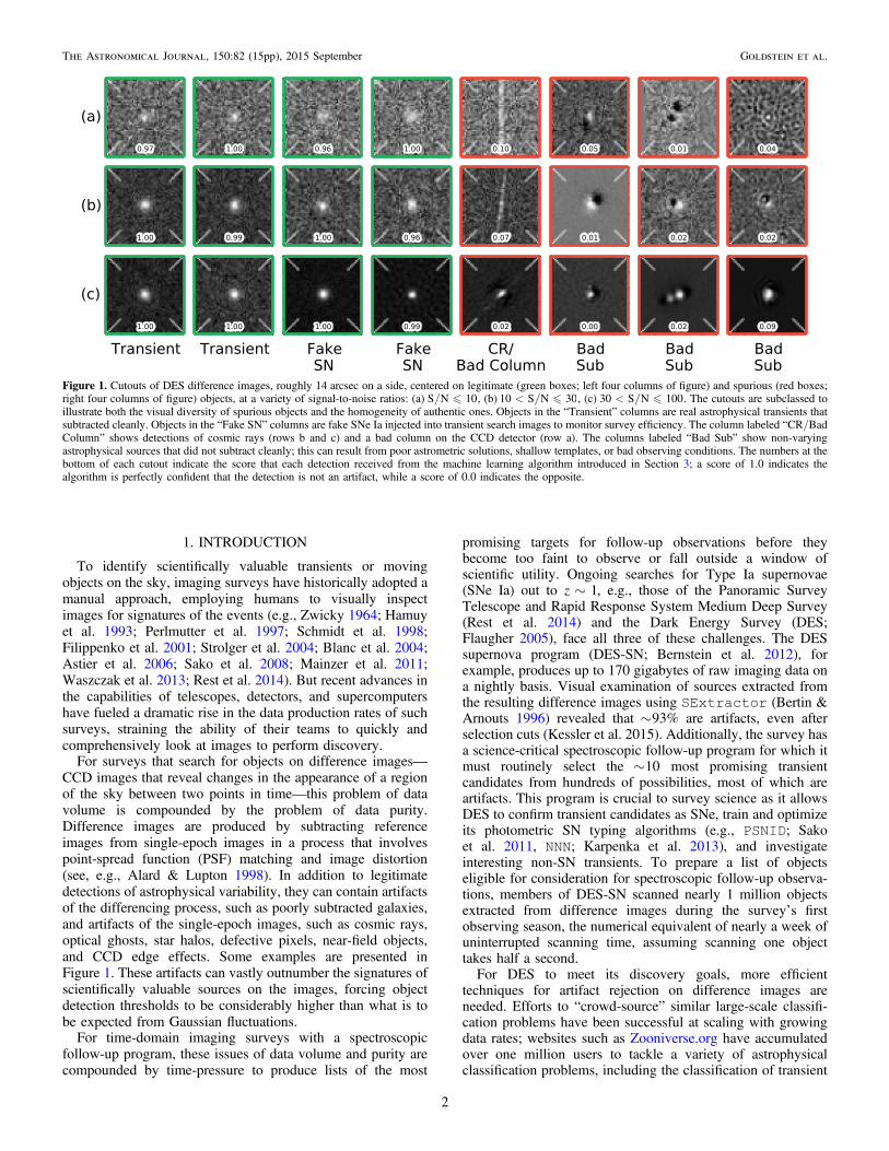
February).A schematic of the pipeline that DES-SN employs to

discover transients is presented in Figure 2. Transient survey

“science images” are single-epoch CCD images from the DES-

SN fields. After the image subtraction step, sources are

extracted using SExtractor. Sources that pass the cuts

described in the Object section of Table 1 are referred to as

“detections.” A “raw candidate” is defined when two or more

detections match to within 1″. A raw candidate is promoted to a

“science candidate” when it passes the NUMEPOCHS require-

ment in Table 1. This selection requirement was imposed to

reject Solar System objects, such as main belt asteroids and

Kuiper Belt objects, which move substantially on images from

night to night. Science candidates are eligible for visual

examination and spectroscopic follow-up observations. During

the observing season, science candidates are routinely photo-

metered, fit with multi-band SN light curve models, visually

inspected, and slated for spectroscopic follow-up.

3. CLASSIFIER DEVELOPMENT

In this section, we describe the development of autoScan.

We present the classifier’s training data set (Section 3.1), its

classification feature set (Section 3.2), and the selection

(Section 3.3), properties (Section 3.4), and optimization

(Section 3.5) of its core classification algorithm.

3.1. Training Data

To make probabilistic statements about the class member-ship of new data, supervised ML classifiers must be trained orfit to existing data whose true class labels are already known.Each data instance is described by numeric classification“features” (see Section 3.2.2); an effective training data setmust approximate the joint feature distributions of all classesconsidered. Objects extracted from difference images canbelong to one of two classes: “Artifacts,” or “Non-artifacts.”Examples of each class must be present in the training set.Failing to include data from certain regions of feature space cancorrode the predictive performance of the classifier in thoseregions, introducing bias into the search that can systematicallydegrade survey efficiency (Richards et al. 2012). Because thetraining set compilation described here took place during thebeginning of Y1, it was complicated by a lack of availablevisually scanned “Non-artifact” sources.Fortunately, labeling data does not necessarily require

humans to visually inspect images. Bloom et al. (2012) discussa variety of methods for labeling detections of variabilityproduced by difference imaging pipelines, including scanningalternatives such as artificial source construction and spectro-scopic follow-up. Scanning, spectroscopy, and using fake dataeach have their respective merits and drawbacks. Scanning islaborious and potentially inaccurate, especially if each datainstance is only examined by one scanner, or if scanners are notwell trained. However, a large group of scanners can quicklylabel a number of detections sufficient to create a training setfor a machine classifier, and Brink et al. (2013) have shownthat the supervised classification algorithm Random Forest,which was ultimately selected for autoScan, is insensitive tomislabeled training data up to a contamination level of 10%.Photometric typing (e.g., Sako et al. 2011) can also be useful

for labeling detections of transients. However, robust photo-metric typing requires well-sampled light curves, which in turn

Figure 2. Schematic of the DES-SN transient detection pipeline. The magnitudes of fake SNe Ia used to monitor survey efficiencyare calibrated using the zero point ofthe images into which they are injected and generated according to the procedure described in Section 3.1. The autoScan step (red box) occurs after selection cutsare applied to objects extracted from difference images and before objects are spatially associated into raw transient candidates. Codes used at specific steps areindicated in parentheses.

4

The Astronomical Journal, 150:82 (15pp), 2015 September Goldstein et al.

require high-cadence photometry of difference image objectsover timescales of weeks or months. This requirement isprohibitive for imaging surveys in their early stages. Further,because photometric typing is an integral part of the spectro-scopic target selection process, by extension new imagingsurveys also have too few detections of spectroscopicallyconfirmed SNe, active galactic nuclei, or variable stars. Nativespectroscopic training samples are therefore impractical sourcesof training data for new surveys.

Artificial source construction is the fastest method forgenerating native detections of non-artifact sources in the earlystages of a survey. Large numbers of artificial transients(“fakes”) can be injected into survey science images, and byconstruction their associated detections are true positives.Difficulties can arise when the joint feature distributions offakes selected for the training set do not approximate the jointfeature distributions of observed transients in production. InDES-SN, SN Ia fluxes from fake SN Ia light curves are overlaidon images near real galaxies. The fake SN Ia light curves aregenerated by the SNANA simulation (Kessler et al. 2009), andthey include true parent populations of stretch and color, arealistic model of intrinsic scatter, a redshift range from 0.1 to1.4, and a galaxy location proportional to surface brightness.On difference images, detections of overlaid fakes are visuallyindistinguishable from real point-source transients and SolarSystem objects moving slowly enough not to streak. All fakeSN Ia light curves are generated and stored prior to the start ofthe survey. The overlay procedure is part of the differenceimaging pipeline, where the SN Ia flux added to the image isscaled by the zero point, spread over nearby pixels using amodel of the PSF, and fluctuated by random Poisson noise.These fakes are used to monitor the single-epoch transientdetection efficiency as well as the candidate efficiency in whichdetections on two distinct nights are required. On average, sixdetections of fake SNe are overlaid on each single-epoch CCD-image.

The final autoScan training set contained detections ofvisually scanned artifacts and artificial sources only. We didnot include detections of photometrically typed transients tominimize the contamination of the “Non-artifact” class with

false positives. Bailey et al. (2007) also used a training set inwhich the “Non-artifact” class consisted largely of artificialsources.With 898,963 training instances in total, the autoScan

training set is the largest used for difference image artifactrejection in production. It was split roughly evenly between“real” and “artifact” labeled instances—454,092 were simu-lated SNe Ia injected onto host galaxies, while the remaining444,871 detections were human-scanned artifacts. Compiling aset of artifacts to train autoScan was accomplished by takinga random sample of the objects that had been scanned asartifacts by humans during an early processing of DES Y1 datawith a pared-down version of the difference imaging pipelinepresented in Figure 2.

3.2. Features and Processing

The supervised learning algorithms we consider in thisanalysis are nonlinear functions that map points representingindividual detections in feature space to points in a space ofobject classes or class probabilities. The second design choicein developing autoScan is therefore to define a suitablefeature space in which to represent the data instances we wishto use for training, validation, and prediction. In this section,we describe the classification features that we computed fromthe raw output of the difference imaging pipeline, as well as thesteps used to pre- and post-process these features.

3.2.1. Data Preprocessing

The primary data sources for autoScan features are51 × 51 pixel object-centered search, template, and differenceimage cutouts. The template and difference image cutouts aresky-subtracted. The search image cutout is sky-subtracted ifand only if it does not originate from a coadded exposure,though this is irrelevant for what follows as no features aredirectly computed from search image pixel values. Photometricmeasurements, SExtractor output parameters, and otherdata sources are also used. Each cutout associated with adetection is compressed to 25 × 25 pixels. The seeing for eachsearch image is usually no less than 1 arcsec, while the DECam

Table 1

DES-SN Object and Candidate Selection Requirements

Set Feature Lower Limit Upper Limit Description

Object MAG L 30.0 Magnitude from SExtractor

A_IMAGE L 1.5 pix. Length of semimajor axis from SExtractor

SPREAD_MODEL L 3 1.0Ss + Star-galaxy separation output parameter from SExtractor Ss is the estimated

SPREAD_MODEL uncertainty

CHISQ L 104 χ2 from PSF-fit to 35 × 35 pixel cutout around object in difference image

SNR 3.5 L Flux from a PSF model fit to a 35 × 35 pixel cutout around the object divided by the

uncertainty from the fit

VETOMAGa 21.0 L Magnitude from SExtractor for use in veto catalog check

VETOTOLa Magnitude-dependent L Separation from nearest object in veto catalog of bright stars

DIPOLE6 L 2 Npix in 35 × 35 pixel object-centered cutout at least 6σ below 0

DIPOLE4 L 20 Npix in 35 × 35 pixel object-centered cutout at least 4σ below 0

DIPOLE2 L 200 Npix in 35 × 35 pixel object-centered cutout at least 2σ below 0

Candidate NUMEPOCHS 2 L Number of distinct nights that the candidate is detected

Note.aThe difference imaging pipeline is expected to produce false positives near bright or variable stars, thus all difference image objects are checked against a “veto”

catalog of known bright and variable stars and are rejected if they are brighter than 21st magnitude and within a magnitude-dependent radius of a veto catalog source.

Thus only one of VETOMAG and VETOTOL must be satisfied for an object to be selected.

5

The Astronomical Journal, 150:82 (15pp), 2015 September Goldstein et al.

pixel scale lies between 0.262 and 0.264 arcsec depending onthe location on the focal plane, so little information is lostduring compression. Although some artifacts are sharper thanthe seeing, we found that using compressed cutouts to computesome features resulted in better performance.

Consider a search, template, or difference image cutoutassociated with a single detection. Let the matrix element Ix y, ofthe 51 × 51 matrix I represent the flux value of the pixel atlocation x y, on the cutout. We adopt the convention of zero-based indexing and the convention that element (0, 0)corresponds to the pixel at the top left-hand corner of thecutout. Let the matrix element Cx y, of the 25 × 25 matrix Crepresent the flux value of the pixel at location x y, on thecompressed cutout. Then C is defined element-wise from I via

ICN

1, 1x y

u i j

x i y j,

0

1

0

1

2 ,2 ( )åå== =

+ +

where Nu is the number of unmasked pixels in the sum. Masked

pixels are excluded from the sum. Only when all four terms in

the sum represent masked pixels is the corresponding pixel

masked in C. Note that matrix elements from the right-hand

column and last row of I never appear in Equation (1).To ensure that the pixel flux values across cutouts are

comparable, we rescale the pixel values of each compressedcutout via

RC Cmed

, 2x yx y

,, ( )

ˆ( )

s=

-

where the matrix element Rx y, of the 25 × 25 matrix R

represents the flux value of the pixel at location x y, on the

compressed, rescaled cutout, and s is a consistent estimator of

the standard deviation of C. We take the median absolute

deviation as a consistent estimator of the standard deviation

(Rousseeuw & Croux 1993), according to

C Cmed med

3

4

31

ˆ(∣ ( )∣)

( )s =-

F- ⎜ ⎟⎛

⎝

⎞

⎠

where 1 3 4 1.48261( )F »- is the reciprocal of the inverse

cumulative distribution for the standard normal distribution

evaluated at 3 4. This is done to ensure that the effects of

defective pixels and cosmic rays nearly perpendicular to the

focal plane are suppressed. We therefore have the following

closed-form expression for the matrix element Rx y, ,

RC C

C C

1

1.4826

med

med med. 4x y

x y,

, ( )

(∣ ( )∣)( )»

-

-

⎡

⎣⎢

⎤

⎦⎥

The rescaling expresses the value of each pixel on the

compressed cutout as the number of standard deviations above

the median. Masked pixels are excluded from the computation

of the median in Equation (4).Finally, an additional rescaling from Brink et al. (2013) is

defined according to

BI I

I

med

max. 5x y

x y

,

, ( )(∣ ∣)

( )=-

The size of B is 51 × 51. We found that using B instead of R or

I to compute certain features resulted in better classifier

performance. Masked pixels are excluded from the computa-

tion of the median in Equation (5).

3.2.2. Feature Library

Two feature libraries were investigated. The first wasprimarily “pixel-based.” For a given object, each matrixelement of the rescaled, compressed search, template, anddifference cutouts was used as a feature. The CCD ID numberof each detection was also used, as DECam has 62 CCDs withspecific artifacts (such as bad columns and hot pixels) as wellas effects that are reproducible on the same CCD depending onwhich field is observed (such as bright stars). The signal-to-noise ratio (S/N) of each detection was also used as a feature.The merits of this feature space include relatively straightfor-ward implementation and computational efficiency. A produc-tion version of this pixel-based classifier was implemented inthe DES-SN transient detection pipeline at the beginning of Y1.In production, it became apparent that the 1877 dimensional40

feature space was dominated by uninformative features, andthat better false positive control could be achieved with a morecompact feature set.We pursued an alternative feature space going forward,

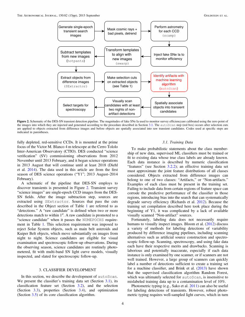
instead using 38 high-level metrics to characterize detections ofvariability. A subset of the features are based on analogs fromBloom et al. (2012) and Brink et al. (2013). In this section, wedescribe the features that are new. We present an at-a-glanceview of the entire autoScan feature library in Table 2.Histograms and contours for the three most important featuresin the final autoScan model (see Section 3.4) appear inFigure 4.

3.2.3. New Features

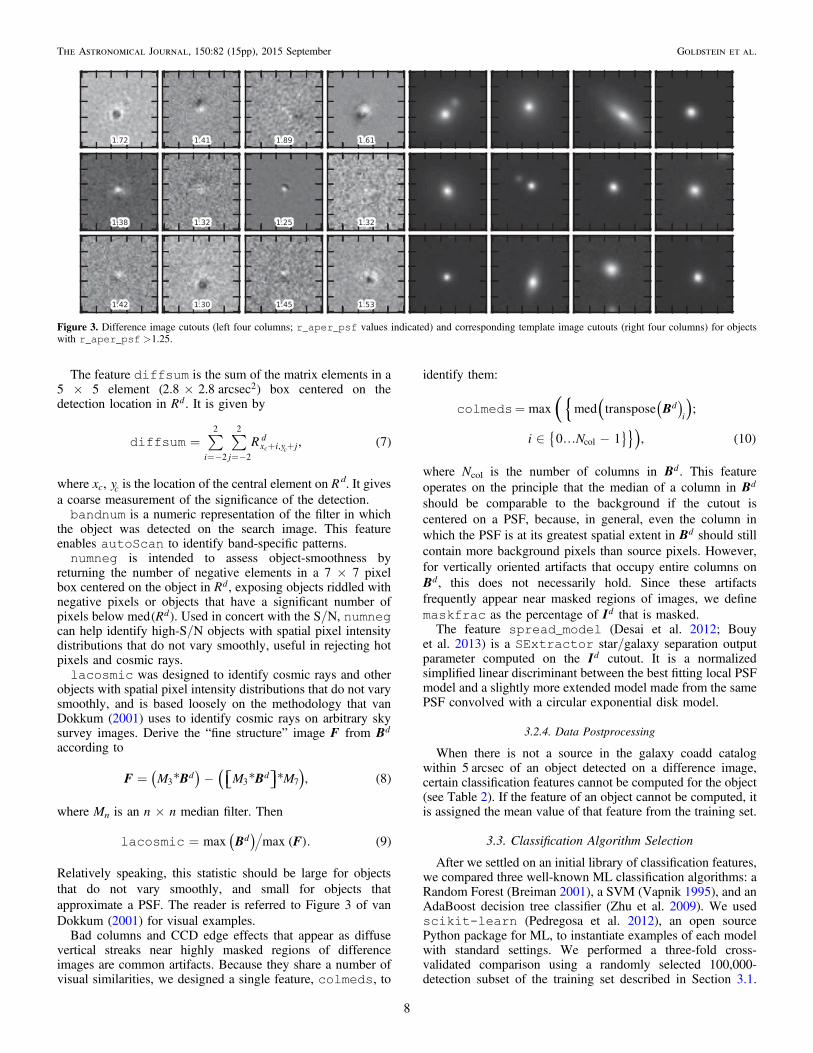
In this section we present new features developed forautoScan. Let the superscripts s t, , and d on matrices definedin the previous section denote search, template, and differenceimages, respectively. The feature r_aper_psf is designed toidentify badly subtracted stars and galaxies on differenceimages caused by poor astrometric alignment between searchand template images. These objects typically appear ondifference images as overlapping circular regions of positiveand negative flux colloquially known as “dipoles.” Examplesare presented in Figure 3. In these cases the typical search-template astrometric misalignment scale is comparable to theFWHM of the PSF, causing the contributions of the negativeand positive regions to the total object flux from a PSF modelfit to be approximately equal in magnitude but opposite in sign,usually with a slight positive excess as the PSF-fit is centeredon the detection location, where the flux is always positive. Thetotal flux from a PSF model fit to a dipole is usually greaterthan but comparable to the average flux per pixel in a five-pixelcircular aperture centered on the detection location on thetemplate image. To this end, let F Iaper, be the flux from a five-pixel circular aperture centered on the location of a detection onthe uncompressed template image. Let F IPSF, be the fluxcomputed by fitting a PSF model to a 35 35´ pixel cutoutcentered on the location of the detection on the uncompressed

40625 pixels on a 25 × 25 pixel cutout ×3 cutouts per detection + 2 non-pixel

features (snr, ccdid) = 1877.

6

The Astronomical Journal, 150:82 (15pp), 2015 September Goldstein et al.

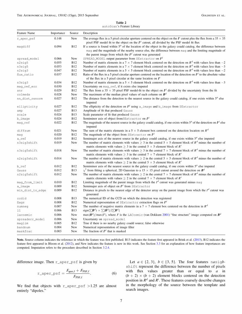
difference image. Then r_aper_psf is given by

F F

F_ _ . 6

I I

I

aper, PSF,

PSF,

( )r aper psf =+

We find that objects with r_aper_psf 1.25> are almost

entirely “dipoles.”

Let a 2, 3{ }Î , b 3, 5{ }Î . The four features nasigb-

shift represent the difference between the number of pixels

with flux values greater than or equal to a in

b b2 2( ) ( )+ ´ + element blocks centered on the detection

position in Rd and Rt. These features coarsely describe changes

in the morphology of the source between the template and

search images.

Table 2

autoScanʼs Feature Library

Feature Name Importance Source Description

r_aper_psf 0.148 New The average flux in a 5 pixel circular aperture centered on the object on the I t cutout plus the flux from a 35 × 35

pixel PSF model fit to the object on the Id cutout, all divided by the PSF model fit flux

magdiff 0.094 B12 If a source is found within 5″ of the location of the object in the galaxy coadd catalog, the difference between

mag and the magnitude of the nearby source else, the difference between mag and the limiting magnitude of

the parent image from which the Id cutout was generated

spread_model 0.066 New SPREAD_MODEL output parameter from SExtractor on Id

n2sig5 0.055 B12 Number of matrix elements in a 7 × 7 element block centered on the detection on R d with values less than −2

n3sig5 0.053 B12 Number of matrix elements in a 7 × 7 element block centered on the detection on R d with values less than −3

n2sig3 0.047 B12 Number of matrix elements in a 5 × 5 element block centered on the detection on Rd with values less than −2

flux_ratio 0.037 B12 Ratio of the flux in a 5 pixel circular aperture centered on the location of the detection on Id to the absolute value

of the flux in a 5 pixel circular at the same location on I t

n3sig3 0.034 B12 Number of matrix elements in a 5 × 5 element block centered on the detection on Rd with values less than −3

mag_ref_err 0.030 B12 Uncertainty on mag_ref, if it exists else imputed

snr 0.029 B12 The flux from a 35 × 35 pixel PSF model-fit to the object on Id divided by the uncertainty from the fit

colmeds 0.028 New The maximum of the median pixel values of each column on Bd

nn_dist_renorm 0.027 B12 The distance from the detection to the nearest source in the galaxy coadd catalog, if one exists within 5″ else

imputed

ellipticity 0.027 B12 The ellipticity of the detection on Id using a_image and b_image from SExtractor

amp 0.027 B13 Amplitude of fit that produced Gauss

scale 0.024 B13 Scale parameter of fit that produced Gauss

b_image 0.024 B12 Semiminor axis of object fromSExtractor on Id

mag_ref 0.022 B12 The magnitude of the nearest source in the galaxy coadd catalog, if one exists within 5″ of the detection on Id else

imputed

diffsum 0.021 New The sum of the matrix elements in a 5 × 5 element box centered on the detection location on Rd

mag 0.020 B12 The magnitude of the object from SExtractor on Id

a_ref 0.019 B12 Semimajor axis of the nearest source in the galaxy coadd catalog, if one exists within 5″ else imputed

n3sig3shift 0.019 New The number of matrix elements with values ≥ 3 in the central 5 × 5 element block of R d minus the number of

matrix elements with values ≥ 3 in the central 5 × 5 element block of R t

n3sig5shift 0.018 New The number of matrix elements with values ≥ 3 in the central 7 × 7 element block of R d minus the number of

matrix elements with values ≥ 3 in the central 7 × 7 element block of R t

n2sig3shift 0.014 New The number of matrix elements with values ≥ 2 in the central 5 × 5 element block of R d minus the number of

matrix elements with values ≥ 2 in the central 5 × 5 element block of R t

b_ref 0.012 B12 Semiminor axis of the nearest source in the galaxy coadd catalog, if one exists within 5″ else imputed

Gauss 0.012 B13 χ2 from fitting a spherical, 2D Gaussian to a 15 × 15 pixel cutout around the detection on Bd

n2sig5shift 0.012 New The number of matrix elements with values ≥ 2 in the central 7 × 7 element block of R d minus the number of

matrix elements with values ≥ 2 in the central 7 × 7 element block of R t

mag_from_limit 0.010 B12 Limiting magnitude of the parent image from which the I d cutout was generated minus mag

a_image 0.009 B12 Semimajor axis of object on Id from SExtractor

min_dist_to_edge 0.009 B12 Distance in pixels to the nearest edge of the detector array on the parent image from which the I d cutout was

generated

ccdid 0.008 B13 The numerical ID of the CCD on which the detection was registered

flags 0.008 B12 Numerical representation of SExtractor extraction flags on Id

numneg 0.007 New The number of negative matrix elements in a 7 × 7 element box centered on the detection in R d

l1 0.006 B13 B B Bsign d d d( ) ∣ ∣ ∣ ∣å ´ å ålacosmic 0.006 New B Fmax maxd( ) ( ), where F is the LACosmic (van Dokkum 2001) “fine structure” image computed on Bd

spreaderr_model 0.006 New Uncertainty on spread_model

maglim 0.005 B12 True if there is no nearby galaxy coadd source; false otherwise

bandnum 0.004 New Numerical representation of image filter

maskfrac 0.003 New The fraction of Id that is masked

Note. Source column indicates the reference in which the feature was first published. B13 indicates the feature first appeared in Brink et al. (2013), B12 indicates the

feature first appeared in Bloom et al. (2012), and New indicates the feature is new in this work. See Section 3.3 for an explanation of how feature importances are

computed. Imputation refers to the procedure described in Section 3.2.4.

7

The Astronomical Journal, 150:82 (15pp), 2015 September Goldstein et al.

The feature diffsum is the sum of the matrix elements in a5 × 5 element (2.8 2.8 arcsec2´ ) box centered on thedetection location in Rd . It is given by

R , 7i j

x i y jd

2

2

2

2

,c c( )diffsum å å=

=- =-+ +

where x y,c c is the location of the central element on R d. It gives

a coarse measurement of the significance of the detection.bandnum is a numeric representation of the filter in which

the object was detected on the search image. This featureenables autoScan to identify band-specific patterns.

numneg is intended to assess object-smoothness byreturning the number of negative elements in a 7 × 7 pixelbox centered on the object in Rd , exposing objects riddled withnegative pixels or objects that have a significant number ofpixels below Rmed d( ). Used in concert with the S/N, numnegcan help identify high-S/N objects with spatial pixel intensitydistributions that do not vary smoothly, useful in rejecting hotpixels and cosmic rays.

lacosmic was designed to identify cosmic rays and otherobjects with spatial pixel intensity distributions that do not varysmoothly, and is based loosely on the methodology that vanDokkum (2001) uses to identify cosmic rays on arbitrary skysurvey images. Derive the “fine structure” image F from Bd

according to

F B BM M M , 8d d3 3 7( )( ) ( )* * *= - ⎡⎣ ⎤⎦

where Mn is an n × n median filter. Then

B Fmax max . 9d( ) ( ) ( )lacosmic =

Relatively speaking, this statistic should be large for objects

that do not vary smoothly, and small for objects that

approximate a PSF. The reader is referred to Figure 3 of van

Dokkum (2001) for visual examples.Bad columns and CCD edge effects that appear as diffuse

vertical streaks near highly masked regions of differenceimages are common artifacts. Because they share a number ofvisual similarities, we designed a single feature, colmeds, to

identify them:

B

i N

max med transpose ;

0 1 , 10

d

i

col

({ ( ))

( )

}{ } ( )

colmeds=

Î ¼ -

where Ncol is the number of columns in Bd . This feature

operates on the principle that the median of a column in Bd

should be comparable to the background if the cutout is

centered on a PSF, because, in general, even the column in

which the PSF is at its greatest spatial extent in Bd should still

contain more background pixels than source pixels. However,

for vertically oriented artifacts that occupy entire columns on

Bd, this does not necessarily hold. Since these artifacts

frequently appear near masked regions of images, we define

maskfrac as the percentage of Id that is masked.The feature spread_model (Desai et al. 2012; Bouy

et al. 2013) is a SExtractor star/galaxy separation outputparameter computed on the Id cutout. It is a normalizedsimplified linear discriminant between the best fitting local PSFmodel and a slightly more extended model made from the samePSF convolved with a circular exponential disk model.

3.2.4. Data Postprocessing

When there is not a source in the galaxy coadd catalogwithin 5 arcsec of an object detected on a difference image,certain classification features cannot be computed for the object(see Table 2). If the feature of an object cannot be computed, itis assigned the mean value of that feature from the training set.

3.3. Classification Algorithm Selection

After we settled on an initial library of classification features,we compared three well-known ML classification algorithms: aRandom Forest (Breiman 2001), a SVM (Vapnik 1995), and anAdaBoost decision tree classifier (Zhu et al. 2009). We usedscikit-learn (Pedregosa et al. 2012), an open sourcePython package for ML, to instantiate examples of each modelwith standard settings. We performed a three-fold cross-validated comparison using a randomly selected 100,000-detection subset of the training set described in Section 3.1.

Figure 3. Difference image cutouts (left four columns; r_aper_psf values indicated) and corresponding template image cutouts (right four columns) for objectswith r_aper_psf 1.25> .

8

The Astronomical Journal, 150:82 (15pp), 2015 September Goldstein et al.

The subset was used to avoid long training times for the SVM.

For a description of cross validation and the metrics used to

evaluate each model, see Sections 4 and 4.2. The results appear

in Figure 5. We found that the performance of all three models

was comparable, but that the Random Forest outperformed the

other models by a small margin. We incorporated the Random

Forest model into autoScan.Random Forests are collections of decision trees, or

cascading sequences of feature-space unit tests, that are

constructed from labeled training data. For an introduction to

decision trees, see Breiman et al. (1984). Random Forests can

be used for predictive classification or regression. During the

construction of a supervised Random Forest classifier, trees in

the forest are trained individually. To construct a single tree,

the training algorithm first chooses a bootstrapped sample of

the training data. The algorithm then attempts to recursively

define a series of binary splits on the features of the training

data that optimally separate the training data into their

constituent classes. During the construction of each node, a

random subsample of features with a user-specified size is

selected with replacement. A fine grid of splits on each feature

is then defined, and the split that maximizes the increase in thepurity of the incident training data is chosen for the node.Two popular metrics for sample-purity are the Gini

coefficient (Gini 1921) and the Shannon entropy (Shan-non 1948). Define the purity of a sample of difference imageobjects to be41

PN

N N, 11

NA

A NA

( )=+

where NNA is the number of non-artifact objects in the sample,

and NA is the number of artifacts in the sample. Note that

P 1= for a sample composed entirely of artifacts, P 0=for a sample composed entirely of non-artifacts, and

P P1 0( )- = for a sample composed entirely of either

artifacts or non-artifacts. Then the Gini coefficient is

P P N NGini 1 . 12A NA( )( ) ( )= - +

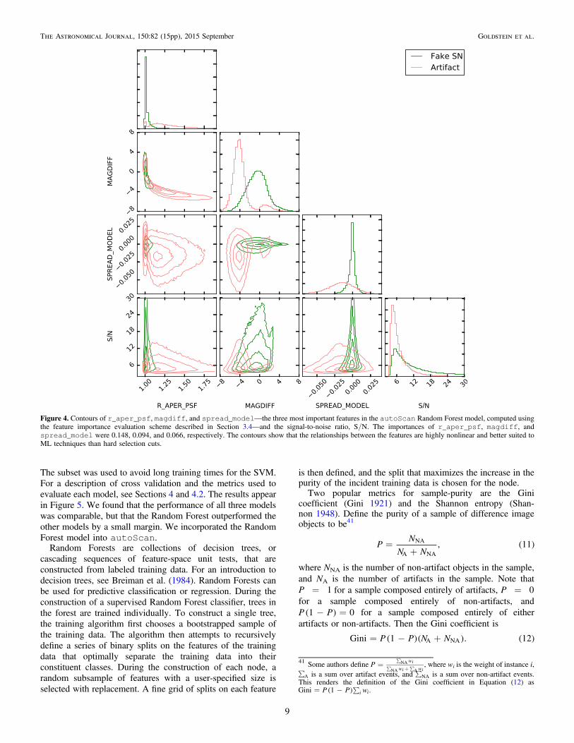
Figure 4. Contours of r_aper_psf, magdiff, and spread_model—the three most important features in the autoScan Random Forest model, computed usingthe feature importance evaluation scheme described in Section 3.4—and the signal-to-noise ratio, S/N. The importances of r_aper_psf, magdiff, andspread_model were 0.148, 0.094, and 0.066, respectively. The contours show that the relationships between the features are highly nonlinear and better suited toML techniques than hard selection cuts.

41Some authors define P

w

w w

i

i i

NA

NA A= å

å +å, where wi is the weight of instance i,

Aå is a sum over artifact events, and NAå is a sum over non-artifact events.This renders the definition of the Gini coefficient in Equation (12) as

P P wGini 1 i i( )= - å .

9

The Astronomical Journal, 150:82 (15pp), 2015 September Goldstein et al.

A tree with a Gini objective function seeks at each node to

minimize the quantity

Gini Gini , 13lc rc ( )+

where Ginilc is the Gini coefficient of the data incident on the

node’s left child, and Ginirc is the Gini coefficient of the data

incident on the node’s right child. If Gini Gini Ginilc rc+ > ,

then no split is performed and the node is declared a terminal

node. The process proceeds identically if another metric is

used, such as the Shannon entropy, the most common

alternative. The Shannon entropy S of a sample of difference

image objects is given by

S p p p plog log , 14NA 2 NA A 2 A( ) ( ) ( )= - -

where pNA is the proportion of non-artifact objects in the

sample, and pA is the proportion of artifacts in the sample.Nodes are generated in this fashion until a maximum depth

or a user-specified measure of node purity is achieved. Thenumber of trees to grow in the forest is left as a free parameterto be set by the user. Training a single Random Forest using theentire ∼900,000 object training sample with the hyperpara-meters selected from the grid search described in Table 3 took4.5~ minutes when the construction of the trees was distributed

across 60 1.6 GHz AMD Opteron 6262 HE processors.Random Forests treat the classes of unseen objects as

unknown parameters that are described probabilistically. Anobject to be classified descends each tree in the forest,beginning at the root nodes. Once a data point arrives at aterminal node, the tree returns the fraction of the traininginstances that reached that node that were labeled “non-artifact.” The output of the trained autoScan Random Forestmodel on a single input data instance is the average of theoutputs of each tree, representing the probability that the objectis not an artifact, henceforth the “autoScan score” or “MLscore.” Ultimately, a score of 0.5 was adopted as the cut τ toseparate real detections of astrophysical variability fromartifacts in the DES-SN data; see Section 4.4 for details. Class

prediction for 200,000 unseen data instances took 9.5 s on asingle 1.6 GHz AMD Opteron 6262 HE processor.

3.4. Feature Importances

Numeric importances can be assigned to the features in atrained forest based on the amount of information theyprovided during training (Breiman et al. 1984). For each treeT in the forest, a tree-specific importance for feature i iscomputed according to

N n B n m n m n , 15i T

n T

i, ch[ ]( ) ( ) ( ) ( ) ( )åz = -Î

where n is an index over nodes in T, N n( ) is the number of

training data points incident on node n, B ni ( ) is 1 if node n

splits on feature i and 0 otherwise, m n( ) is the value of the

objective function (usually the Gini coefficient or the Shannon

entropy; see Section 3.3) applied to the the training data

incident on node n, and m nch ( ) is the sum of the values of the

objective function applied to the node’s left and right children.

The global importance of feature i is the average of the tree-

specific importances:

IN

1, 16i

T T

i T, ( )åz=

where NT is the number of trees in the forest. In this article,

importances are normalized to sum to unity.

3.5. Optimization

The construction of a Random Forest is governed by anumber of free parameters called hyperparameters. Thehyperparameters of the Random Forest implementation usedin this work are n_estimators, the number of decision treesin the forest, criterion, the function that measures thequality of a proposed split at a given tree node, max_fea-tures, the number of features to randomly select whenlooking for the best split at a given tree node, max_depth, themaximum depth of a tree, and min_samples_split, theminimum number of samples required to split an internal node.We performed a 3-fold cross-validated (see Section 4.2) grid

search over the space of Random Forest hyperparametersdescribed in Table 3. A total of 1884 trainings were performed.The best classifier had 100 trees, used the Shannon entropyobjective function, chose 6 features for each split, required atleast 3 samples to split a node, and had unlimited depth, and itwas incorporated into the code. Recursive feature elimination(Brink et al. 2013) was explored to improve the performance of

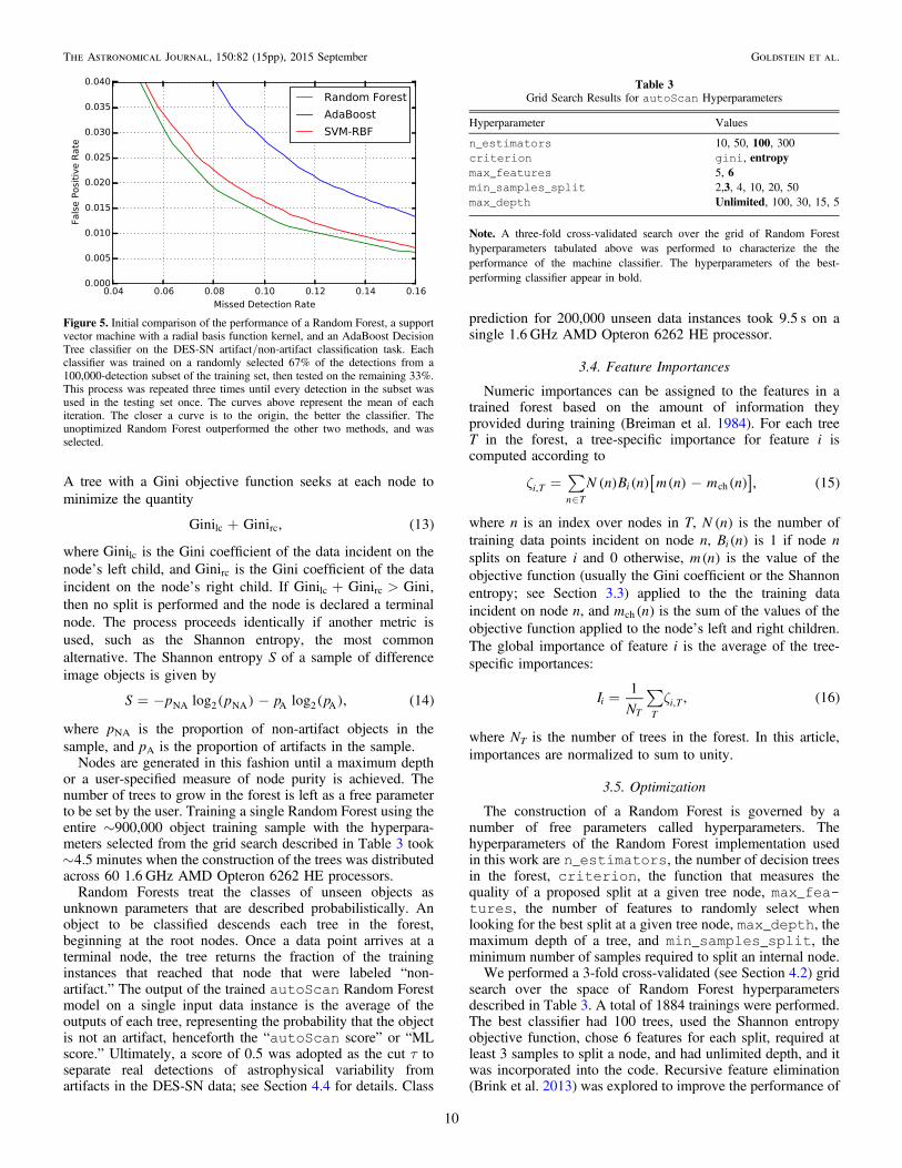
Figure 5. Initial comparison of the performance of a Random Forest, a supportvector machine with a radial basis function kernel, and an AdaBoost DecisionTree classifier on the DES-SN artifact/non-artifact classification task. Eachclassifier was trained on a randomly selected 67% of the detections from a100,000-detection subset of the training set, then tested on the remaining 33%.This process was repeated three times until every detection in the subset wasused in the testing set once. The curves above represent the mean of eachiteration. The closer a curve is to the origin, the better the classifier. Theunoptimized Random Forest outperformed the other two methods, and wasselected.

Table 3

Grid Search Results for autoScan Hyperparameters

Hyperparameter Values

n_estimators 10, 50, 100, 300

criterion gini, entropy

max_features 5, 6

min_samples_split 2,3, 4, 10, 20, 50

max_depth Unlimited, 100, 30, 15, 5

Note. A three-fold cross-validated search over the grid of Random Forest

hyperparameters tabulated above was performed to characterize the the

performance of the machine classifier. The hyperparameters of the best-

performing classifier appear in bold.

10

The Astronomical Journal, 150:82 (15pp), 2015 September Goldstein et al.

the classifier, but we found that it provided no statisticallysignificant performance improvement.

4. PERFORMANCE

In this section, we describe performance of autoScan on arealistic classification task and the effect of the code on theDES-SN transient candidate scanning load. Performancestatistics for the classification task were measured usingproduction Y1 data, whereas candidate-level effects weremeasured using a complete reprocessing of Y1 data using anupdated difference imaging pipeline. The reprocessed detectionpool differed significantly from its production counterpart,providing a out-of-sample data set for benchmarking the effectsof the code on the scanning load.42

4.1. Performance Metrics

The performance of a classifier on an n-class task iscompletely summarized by the corresponding n × n confusionmatrix , also known as a contingency table or error matrix.The matrix element ij represents the number of instances fromthe task’s validation set with ground truth class label j that werepredicted to be members of class i. A schematic 2 × 2confusion matrix for the autoScan classification task isshown in Figure 6.

From the confusion matrix, several classifier performancemetrics can be computed. Two that frequently appear in theliterature are the False Positive Rate (FPR) and the MissedDetection Rate (MDR; also known as the False Negative Rateor False Omission Rate). Using the notation from Figure 6, theFPR is defined by:

F

F TFPR , 17

p

p n

( )=+

and the MDR by

F

T FMDR . 18

n

p n

( )=+

For autoScan, the FPR represents the fraction of artifacts in

the validation set that are predicted to be legitimate detections

of astrophysical variability. The MDR represents the fraction of

non-artifacts in the task’s validation set that are predicted to be

artifacts. Another useful metric is the efficiency or true positive

rate,

T

T F, 19

p

p n

( ) =+

which represents the fraction of non-artifacts in the sample that

are classified correctly. For the remainder of this study, we

often refer to the candidate-level efficiency measured on fake

SNe Ia, F (see Section 4.4).Finally, the receiver operating characteristic (ROC) is a

graphical tool for visualizing the performance of a classifier. Itdisplays FPR as a function of MDR, both of which areparametric functions of τ, the autoScan score that onechooses to delineate the boundary between “non-artifacts” and“artifacts.” One can use the ROC to determine the location atwhich the trade-off between the FPR and MDR is optimal forthe survey at hand, a function of both the scanning load and thepotential bias introduced by the classifier, then solve for thecorresponding τ. By benchmarking the performance of theclassifier using the the ROC, one can paint a complete pictureof its performance that can also serve as a statistical guaranteeon performance in production, assuming a validation set and aproduction data set that are identically distributed in featurespace, and that detections are scanned individually inproduction (see Section 4.4).

4.2. Classification Task

We used stratified five-fold cross-validation to test theperformance of autoScan. Cross validation is a technique forassessing how the results of a statistical analysis will generalizeto an independent data set. In a k-fold cross-validated analysis,a data set is partitioned into k disjoint subsets. k iterations oftraining and testing are performed. During the ith iteration,subset i is held out as a “validation” set of labeled datainstances that are not included in the training sample, and theunion of the remaining k 1- subsets is passed to the classifieras a training set. The classifier is trained and its predictiveperformance on the validation set is recorded. In standard k-fold cross-validation, the partitioning of the original data setinto disjoint subsets is done by drawing samples at randomwithout replacement from the original data set. But in astratified analysis, the drawing is performed subject to theconstraint that the distribution of classes in each subset be thesame as the distribution of classes in the original data set.Cross-validation is useful because it enables one to characterizehow a classifier’s performance varies with respect to changes inthe composition of training and testing data sets, helpingquantify and control “generalization error.”

4.3. Results

Figure 7 shows the ROCs that resulted from each round ofcross-validation. We report that autoScan achieved an

Figure 6. Schematic confusion matrix for the autoScan classification task.Each matrix element ij represents the number of instances from the task’s

validation set with ground truth class label j that were predicted to be membersof class i.

42Although the re-processing of data through the difference imaging pipeline

from the raw images is not useful for getting spectra of live transients, it is quiteuseful for acquiring host-galaxy targets for previously missed transients and istherefore performed regularly as pipeline improvements are made.

11

The Astronomical Journal, 150:82 (15pp), 2015 September Goldstein et al.

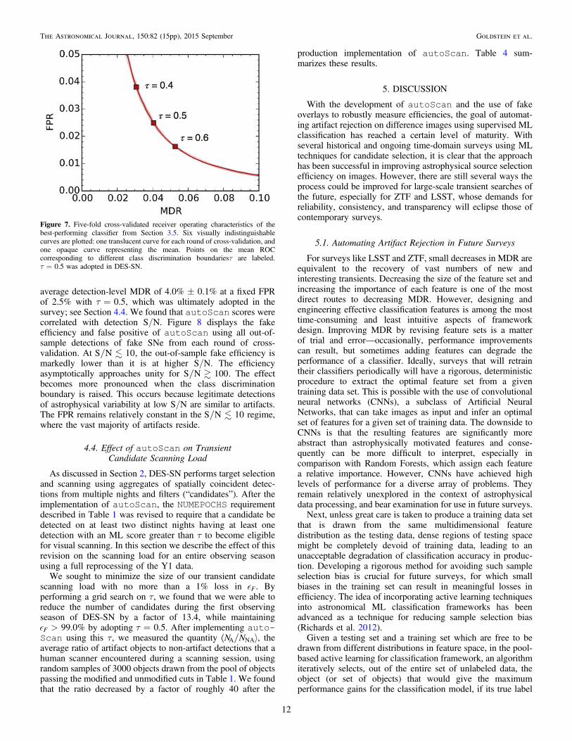
average detection-level MDR of 4.0% ± 0.1% at a fixed FPRof 2.5% with 0.5t = , which was ultimately adopted in thesurvey; see Section 4.4. We found that autoScan scores werecorrelated with detection S/N. Figure 8 displays the fakeefficiency and false positive of autoScan using all out-of-sample detections of fake SNe from each round of cross-validation. At S N 10 , the out-of-sample fake efficiency ismarkedly lower than it is at higher S/N. The efficiencyasymptotically approaches unity for S N 100 . The effectbecomes more pronounced when the class discriminationboundary is raised. This occurs because legitimate detectionsof astrophysical variability at low S/N are similar to artifacts.The FPR remains relatively constant in the S N 10 regime,where the vast majority of artifacts reside.

4.4. Effect of autoScan on TransientCandidate Scanning Load

As discussed in Section 2, DES-SN performs target selectionand scanning using aggregates of spatially coincident detec-tions from multiple nights and filters (“candidates”). After theimplementation of autoScan, the NUMEPOCHS requirementdescribed in Table 1 was revised to require that a candidate bedetected on at least two distinct nights having at least onedetection with an ML score greater than τ to become eligiblefor visual scanning. In this section we describe the effect of thisrevision on the scanning load for an entire observing seasonusing a full reprocessing of the Y1 data.

We sought to minimize the size of our transient candidatescanning load with no more than a 1% loss in F . Byperforming a grid search on τ, we found that we were able toreduce the number of candidates during the first observingseason of DES-SN by a factor of 13.4, while maintaining

99.0%F > by adopting 0.5t = . After implementing auto-

Scan using this τ, we measured the quantity N NA NA⟨ ñ, theaverage ratio of artifact objects to non-artifact detections that ahuman scanner encountered during a scanning session, usingrandom samples of 3000 objects drawn from the pool of objectspassing the modified and unmodified cuts in Table 1. We foundthat the ratio decreased by a factor of roughly 40 after the

production implementation of autoScan. Table 4 sum-marizes these results.

5. DISCUSSION

With the development of autoScan and the use of fakeoverlays to robustly measure efficiencies, the goal of automat-ing artifact rejection on difference images using supervised MLclassification has reached a certain level of maturity. Withseveral historical and ongoing time-domain surveys using MLtechniques for candidate selection, it is clear that the approachhas been successful in improving astrophysical source selectionefficiency on images. However, there are still several ways theprocess could be improved for large-scale transient searches ofthe future, especially for ZTF and LSST, whose demands forreliability, consistency, and transparency will eclipse those ofcontemporary surveys.

5.1. Automating Artifact Rejection in Future Surveys

For surveys like LSST and ZTF, small decreases in MDR areequivalent to the recovery of vast numbers of new andinteresting transients. Decreasing the size of the feature set andincreasing the importance of each feature is one of the mostdirect routes to decreasing MDR. However, designing andengineering effective classification features is among the mosttime-consuming and least intuitive aspects of frameworkdesign. Improving MDR by revising feature sets is a matterof trial and error—occasionally, performance improvementscan result, but sometimes adding features can degrade theperformance of a classifier. Ideally, surveys that will retraintheir classifiers periodically will have a rigorous, deterministicprocedure to extract the optimal feature set from a giventraining data set. This is possible with the use of convolutionalneural networks (CNNs), a subclass of Artificial NeuralNetworks, that can take images as input and infer an optimalset of features for a given set of training data. The downside toCNNs is that the resulting features are significantly moreabstract than astrophysically motivated features and conse-quently can be more difficult to interpret, especially incomparison with Random Forests, which assign each featurea relative importance. However, CNNs have achieved highlevels of performance for a diverse array of problems. Theyremain relatively unexplored in the context of astrophysicaldata processing, and bear examination for use in future surveys.Next, unless great care is taken to produce a training data set

that is drawn from the same multidimensional featuredistribution as the testing data, dense regions of testing spacemight be completely devoid of training data, leading to anunacceptable degradation of classification accuracy in produc-tion. Developing a rigorous method for avoiding such sampleselection bias is crucial for future surveys, for which smallbiases in the training set can result in meaningful losses inefficiency. The idea of incorporating active learning techniquesinto astronomical ML classification frameworks has beenadvanced as a technique for reducing sample selection bias(Richards et al. 2012).Given a testing set and a training set which are free to be

drawn from different distributions in feature space, in the pool-based active learning for classification framework, an algorithmiteratively selects, out of the entire set of unlabeled data, theobject (or set of objects) that would give the maximumperformance gains for the classification model, if its true label

Figure 7. Five-fold cross-validated receiver operating characteristics of thebest-performing classifier from Section 3.5. Six visually indistinguishablecurves are plotted: one translucent curve for each round of cross-validation, andone opaque curve representing the mean. Points on the mean ROCcorresponding to different class discrimination boundariesτ are labeled.τ = 0.5 was adopted in DES-SN.

12

The Astronomical Journal, 150:82 (15pp), 2015 September Goldstein et al.

were known. The algorithm then solicits a user to manuallyinput the class of the object under consideration, and then theobject is automatically incorporated into future training sets toimprove upon the original classifier. Under this paradigm,human scanners would play the valuable role of helping theclassifier learn from its mistakes, and each human hour spentvetting data would immediately carry scientific return. Activelearning could produce extremely powerful classifiers overshort timescales when used in concert with generative modelsfor training data. Instead of relying on historical data to trainartifact rejection algorithms during commissioning phases,experiments like LSST could use generative models for surveyobservations to simulate new data sets. After training aclassifier using simulated data, in production active learningcould be used to automatically fill in gaps in classifierknowledge and augment predictive accuracy.

In this work, we used a generative model of SN Iaobservations—overlaying fake SNe Ia onto real host

galaxies—to produce the “Non-artifact” component of ourtraining data set. However, the nearly 500,000 artifacts inour training set were human-scanned, implying that futuresurveys will still need to do a great deal of scanning beforebeing able to get an ML classifier off the ground. A newsurvey should not intentionally alter the pipeline to produceartifacts during commissioning, as it is crucial that theunseen data be drawn from the same feature distributions asthe training data. For surveys with N N 100A NA⟨ ñ , Brinket al. (2013) showed that a robust artifact library can beprepared by randomly sampling from all detections ofvariability produced by the difference imaging pipeline.For surveys or pipelines that do not produce as manyartifacts, some initial scanning to produce a few 104-artifactlibrary from commissioning data should be sufficient toproduce an initial training set (Brink et al. 2013; du Buissonet al. 2014).

5.2. Eliminating Spurious Candidates

Using a two-night trigger, some spurious science candidatescan be created due to nightly variations in astrometry,observing conditions, and repeatedly imaged source bright-nesses that cause night-to-night fluctuations in the appearanceof candidates on difference images. These variations lead to aspread of ML scores for a given candidate. As an observingseason progress, artifacts can accumulate large numbers ofdetections via repeated visits. Although for a typical artifact thevast majority of detections fail the ML requirement, thefluctuations in ML scores can cause a small fraction of thedetections to satisfy the autoScan requirement. Figure 9shows an example of this effect.Mitigating the buildup of spurious multi-night candidates

could be achieved by implementing a second ML classificationframework that takes as input multi-night information,

Figure 8. Object-level fake efficiency and FPR as a function of S/N, at several autoScan score cuts. The S/N is computed by dividing the flux from a PSF model fitto a 35 × 35 pixel cutout around the object in the difference image by the uncertainty from the fit. The artifact rejection efficiency and MDR are 1 minus the falsepositive rate and fake efficiency, respectively. The fake efficiency of autoScan degrades at low S/N, whereas the false positive rate is relatively constant in the S/Nregime not dominated by small number statistics. τ = 0.5 (bold) was adopted in DES-SN.

Table 4

autoScan DES Y1 Reprocessing Results

No ML ML (τ = 0.5 ) ML/No ML

Nca 100,450 7489 0.075

N NA NA⟨ ñb 13 0.34 0.027

F c 1.0 0.990 0.990

Notes.aTotal number of science candidates discovered.

bAverage ratio of artifact to non-artifact detections in human scanning pool

determined from scanning 3000 randomly selected detections from all science

candidate detections.cautoScan candidate-level efficiency for fake SNe Ia.

13

The Astronomical Journal, 150:82 (15pp), 2015 September Goldstein et al.

including the detection-level output of autoScan, to predictwhether a given science candidate represents a bona-fideastrophysical source. Training data compilation could beperformed by randomly selecting time-contiguous strings ofdetections from known candidates. The lengths of the stringscould be drawn from a distribution specified during frameworkdevelopment. Candidate-level features could characterize thetemporal variation of detection level features, such as thehighest and lowest night-to-night shifts in autoScan score,magnitude, and astrometric uncertainty.

D.A.G. thanks Josh Bloom for productive conversations andan anonymous referee for comments that improved the paper.We are grateful for the extraordinary contributions of our CTIOcolleagues and the DES Camera, Commissioning and ScienceVerification teams for achieving excellent instrument andtelescope conditions that have made this work possible. Thesuccess of this project also relies critically on the expertise anddedication of the DES Data Management organization. Fundingfor DES projects has been provided by the U.S. Department ofEnergy, the U.S. National Science Foundation, the Ministry ofScience and Education of Spain, the Science and TechnologyFacilities Council of the United Kingdom, the Higher EducationFunding Council for England, the National Center for Super-computing Applications at the University of Illinois at Urbana-Champaign, the Kavli Institute of Cosmological Physics at theUniversity of Chicago, Financiadora de Estudos e Projetos,Fundação Carlos Chagas Filho de Amparo á Pesquisa do Estadodo Rio de Janeiro, Conselho Nacional de DesenvolvimentoCientífico e Tecnológico and the Ministério da Ciência eTecnologia, the Deutsche Forschungsgemeinschaft, and thecollaborating institutions in the Dark Energy Survey. Thecollaborating institutions are Argonne National Laboratory, theUniversity of California, Santa Cruz, the University of Cam-bridge, Centro de Investigaciones Energeticas, Medioambien-tales y Tecnologicas-Madrid, the University of Chicago,University College London, the DES-Brazil Consortium, theEidgenössische Tecnische Hochschule (ETH) Zürich, FermiNational Accelerator Laboratory, the University of Edinburgh,

the University of Illinois at Urbana-Champaign, the Institut deCiencies de l’Espai (IEEC/CSIC), the Intitut de Fisica d’AltesEnergies, Lawrence Berkeley National Laboratory, the Ludwig-Maximilians Universität and the associated Excellence ClusterUniverse, the University of Michigan, the National OpticalAstronomy Observatory, the University of Nottingham, the OhioState University, the University of Pennsylvania, the Universityof Portsmouth, SLAC National Acclerator Laboratory, StanfordUniversity, the University of Sussex, and Texas A&MUniversity. This research used resources of the National EnergyResearch Scientific Computing Center, a DOE Office of ScienceUser Facility supported by the Office of Science of the U.S.Department of Energy under Contract No. DE-AC02-05CH11231. Figure 4 was generated with a modified versionof triangle.py (Foreman-Mackey et al. 2014). A.C.R.acknowledges financial support provided by the PAPDRJCAPES/FAPERJ Fellowship. F.S. acknowledges financialsupport provided by CAPES under contract No. 3171-13-2.The DES participants from Spanish institutions are partiallysupported by MINECO under grants AYA2012-39559,ESP2013-48274, FPA2013-47986, and Centro de ExcelenciaSevero Ochoa SEV-2012-0234, some of which include ERDFfunds from the European Union.

REFERENCES

Alard, C., & Lupton, R. H. 1998, ApJ, 503, 325Albrecht, A., Bernstein, G., Cahn, R., et al. 2006, arXiv:astro-ph/0609591Aldering, G., Adam, G., Antilogus, P., et al. 2002, Proc. SPIE, 4836, 61Aragon, C. R., Bailey, S. J., Poon, S., Runge, K., & Thomas, R. C. 2008,

JPhCS, 125, 012091Astier, P., Guy, J., Regnault, N., et al. 2006, A&A, 447, 31Bailey, S., Aragon, C., Romano, R., et al. 2007, ApJ, 665, 1246Baltay, C., Rabinowitz, D., Andrews, P., et al. 2007, PASP, 119, 1278Banerji, M., Lahav, O., Lintott, C. J., et al. 2010, MNRAS, 406, 342Bernstein, J. P., Kessler, R., Kuhlmann, S., et al. 2012, ApJ, 753, 152Bertin, E., & Arnouts, S. 1996, A&AS, 117, 393Blanc, G., Afonso, C., Alard, C., et al. 2004, A&A, 423, 881Bloom, J. S., Richards, J. W., Nugent, P. E., et al. 2012, PASP, 124, 1175Bouy, H., Bertin, E., Moraux, E., et al. 2013, A&A, 554, AA101Breiman, L. 2001, Machine Learning, 45, 5

Figure 9. Twenty-four consecutively observed difference image cutouts of a poorly subtracted galaxy that was wrongly identified as a transient. The autoScan scoreof each detection appears at the bottom of each cutout. The mis-identification occurred because on two nights the candidate had a detection that received a score abovean autoScan class discrimination boundary τ = 0.4 used during early code tests (green boxes). Night-to-night variations in observing conditions, data reduction, andimage subtraction can cause detections of artifacts to appear real. If a two-night trigger is used, spurious “transients” like this one can can easily accumulate as a seasongoes on. Consequently, care must be taken when using an artifact rejection framework that scores individual detections to make statements about aggregates ofdetections. Each image is labeled with the observation date and filter for the image, in the format YYYYMMDD-filter.

14

The Astronomical Journal, 150:82 (15pp), 2015 September Goldstein et al.

Breiman, L., Friedman, J., Stone, C. J., & Olshen, R. A. 1984, Classificationand Regression Trees (London: CRC Press)

Brink, H., Richards, J. W., Poznanski, D., et al. 2013, MNRAS, 435, 1047du Buisson, L., Sivanandam, N., Bassett, B. A., & Smith, M. 2014,

arXiv:1407.4118Desai, S., Armstrong, R., Mohr, J. J., et al. 2012, ApJ, 757, 83Diehl, H. T. (for the Dark Energy Survey Collaboration) 2012, PhPro, 37, 1332Diehl, H. T., Abbott, T. M., Annis, J., et al. 2014, Proc. SPIE, 9149, 91490VFilippenko, A. V., Li, W. D., Treffers, R. R., & Modjaz, M. 2001, in ASP

Conf. Ser., 246, Spectroscopy Challenge of Photoionized Plasmas, ed.G. Ferland & D. Wolf Savin (San Francisco, CA: ASP), 121

Flaugher, B. 2005, IJMPA, 20, 3121Flaugher, B., Abbott, T. M. C., Angstadt, R., et al. 2012, Proc. SPIE, 8446,

844611Flaugher, B., Diehl, H. T., Honscheid, K., et al. 2015, arXiv:1504.02900Foreman-Mackey, D., Price-Whelan, A., Ryan, G., et al. 2014, ZenodoFrieman, J. A., Bassett, B., Becker, A., et al. 2008, AJ, 135, 338Gini, C. 1921, Econ. J., 31, 124Hamuy, M., Maza, J., Phillips, M. M., et al. 1993, AJ, 106, 2392Ivezić, Ż, Connolly, A., VanderPlas, J., & Gray, A. 2013, Statistics, Data

Mining, and Machine Learning in Astronomy (Princeton, NJ: PrincetonUniv. Press)

Karpenka, N. V., Feroz, F., & Hobson, M. P. 2013, MNRAS, 429, 1278Kessler, R., Bernstein, J. P., Cinabro, D., et al. 2009, PASP, 121, 1028

LSST Science Collaboration 2009, arXiv:0912.0201Mainzer, A., Bauer, J., Grav, T., et al. 2011, ApJ, 731, 53Pedregosa, F., Varoquaux, G., Gramfort, A., et al. 2012, arXiv:1201.0490Perlmutter, S., Aldering, G., Deustua, S., et al. 1997, AAS, 29, 1351Rest, A., Scolnic, D., Foley, R. J., et al. 2014, ApJ, 795, 44Richards, J. W., Starr, D. L., Brink, H., et al. 2012, ApJ, 744, 192Richards, J. W., Starr, D. L., Butler, N. R., et al. 2011, ApJ, 733, 10Rousseeuw, P. J., & Croux, C. 1993, J. Am. Stat. Assoc., 88, 1273Sako, M., Bassett, B., Becker, A., et al. 2008, AJ, 135, 348Sako, M., Bassett, B., Connolly, B., et al. 2011, ApJ, 738, 162Schmidt, B. P., Suntzeff, N. B., Phillips, M. M., et al. 1998, ApJ, 507, 46Shannon, C. E. 1948, BSTJ, 27, 379Smith, R. M., Dekany, R. G., Bebek, C., et al. 2014, Proc. SPIE, 9147, 914779Smith, A. M., Lynn, S., Sullivan, M., et al. 2011, MNRAS, 412, 1309Strolger, L.-G., Riess, A. G., Dahlen, T., et al. 2004, ApJ, 613, 200van Dokkum, P. G. 2001, PASP, 113, 1420Vapnik, V. 1995, The Nature of Statistical Learning Theory (New York:

Springer)Waszczak, A., Ofek, E. O., Aharonson, O., et al. 2013, MNRAS, 433, 3115Willsky, A. S., Wornell, G. W., & Shapiro, J. H. 2003, Stochastic Processes,

Detection, and Estimation (Course notes for MIT 6.432)Wright, D. E., Smartt, S. J., Smith, K. W., et al. 2015, MNRAS, 449, 451Zhu, J., Zou, H., Rosset, S., & Hastie, T. 2009, SII, 2.3, 349Zwicky, F. 1964, AnAp, 27, 300

15

The Astronomical Journal, 150:82 (15pp), 2015 September Goldstein et al.