Embed Size (px)
Citation preview

Automated Pricing Agents in the On-Demand
Economy
Tony WuAnthony D. Joseph, Ed.Stuart J. Russell, Ed.
Electrical Engineering and Computer SciencesUniversity of California at Berkeley
Technical Report No. UCB/EECS-2016-57
http://www.eecs.berkeley.edu/Pubs/TechRpts/2016/EECS-2016-57.html
May 12, 2016

Copyright © 2016, by the author(s).All rights reserved.
Permission to make digital or hard copies of all or part of this work forpersonal or classroom use is granted without fee provided that copies arenot made or distributed for profit or commercial advantage and that copiesbear this notice and the full citation on the first page. To copy otherwise, torepublish, to post on servers or to redistribute to lists, requires prior specificpermission.
Acknowledgement
I would like to thank both Professor Anthony Joseph and Professor StuartRussell for advising me on this paper. I am grateful for Professor Joseph'ssupport not only on this research project but on my previous researchprojects in the UC Berkeley SCRUB Lab. I am also thankful for ProfessorRussell's advice on the reinforcement learning aspects of this paper andteaching a wonderful CS294-125 Human Compatible AI class. I would alsolike to thank family and friends for their continuous support. I also thank mycoworkers at Dray for supporting me through completing my Mastersdegree alongside startup work. I am excited to integrate Dray's marketplacedata with the pricing algorithms explored in this paper.


Automated Pricing Agents in the On-Demand Economy
Copyright 2016by
Tony Wu

Acknowledgments
I would like to thank both Professor Anthony Joseph and Professor Stuart Russell for advis-ing me on this paper. I am grateful for Professor Joseph’s support not only on this researchproject but on my previous research projects in the UC Berkeley SCRUB Lab. I am alsothankful for Professor Russell’s advice on the reinforcement learning aspects of this paperand teaching a wonderful CS294-125 Human Compatible AI class. I would also like to thankfamily and friends for their continuous support. I also thank my coworkers at Dray for sup-porting me through completing my Masters degree alongside startup work. I am excited tointegrate Dray’s marketplace data with the pricing algorithms explored in this paper.

Abstract
Automated Pricing Agents in the On-Demand Economy
by
Tony Wu
Master of Science in Electrical Engineering and Computer Science
University of California, Berkeley
We present this thesis to study and build automated pricing engines that work in on-demand economies. The task of determining market prices is especially challenging in anon-demand marketplace because of frequently fluctuating supply and demand. An automatedpricing agent provides reactive real-time prices. To evaluate different types of automatedpricing models, we build an on-demand marketplace simulation. By using research on humanbehavior, we create customer and supplier agent models that interact within the simulation.Afterwards, we run market experiments using various pricing algorithms. We introducethe concept of applying reinforcement learning to generate dynamic prices, and we evaluateour reinforcement learning agent’s performance relative to that of other simpler pricingalgorithms. Performance is measured not only in terms of profit, but also in metrics thatdetermine customer and supplier retention.

i
Contents
Contents i
1 Market Overview 31.1 Marketplaces . . . . . . . . . . . . . . . . . . . . . . . . . . . . . . . . . . . 31.2 Market players . . . . . . . . . . . . . . . . . . . . . . . . . . . . . . . . . . 41.3 Differences from other marketplaces . . . . . . . . . . . . . . . . . . . . . . . 41.4 Rise of automated pricing systems . . . . . . . . . . . . . . . . . . . . . . . . 51.5 Relevant literature review . . . . . . . . . . . . . . . . . . . . . . . . . . . . 6
2 Pricing Simulation Setup 82.1 Overview . . . . . . . . . . . . . . . . . . . . . . . . . . . . . . . . . . . . . . 82.2 Agent preferences . . . . . . . . . . . . . . . . . . . . . . . . . . . . . . . . . 92.3 Population models . . . . . . . . . . . . . . . . . . . . . . . . . . . . . . . . 102.4 Action models . . . . . . . . . . . . . . . . . . . . . . . . . . . . . . . . . . . 112.5 Modeling different agent types . . . . . . . . . . . . . . . . . . . . . . . . . . 122.6 Modeling cost . . . . . . . . . . . . . . . . . . . . . . . . . . . . . . . . . . . 132.7 Setting the initial price . . . . . . . . . . . . . . . . . . . . . . . . . . . . . . 14
3 Dynamic Pricing Algorithms 163.1 Overview . . . . . . . . . . . . . . . . . . . . . . . . . . . . . . . . . . . . . . 163.2 Static pricing . . . . . . . . . . . . . . . . . . . . . . . . . . . . . . . . . . . 163.3 Proportional pricing . . . . . . . . . . . . . . . . . . . . . . . . . . . . . . . 163.4 Batch update pricing . . . . . . . . . . . . . . . . . . . . . . . . . . . . . . . 173.5 Reinforcement learning . . . . . . . . . . . . . . . . . . . . . . . . . . . . . . 17
4 Short Term Simulations 194.1 Overview . . . . . . . . . . . . . . . . . . . . . . . . . . . . . . . . . . . . . . 194.2 Surge pricing . . . . . . . . . . . . . . . . . . . . . . . . . . . . . . . . . . . 194.3 Comparison . . . . . . . . . . . . . . . . . . . . . . . . . . . . . . . . . . . . 21
5 Long Term Simulations 305.1 Overview . . . . . . . . . . . . . . . . . . . . . . . . . . . . . . . . . . . . . . 30

5.2 Comparison . . . . . . . . . . . . . . . . . . . . . . . . . . . . . . . . . . . . 31
6 Future Work 38
7 Conclusion 40
Bibliography 41

3
Chapter 1
Market Overview
1.1 Marketplaces
Many types of marketplaces exist in the world today, each with their own pricing strategies.This paper focuses on pricing in the “on-demand” economy. We can define the on-demandeconomy as a marketplace where companies provide fulfillment of customer demand via theimmediate provisioning of goods and services. On-demand services have become increas-ingly popular with improvements in Internet availability, mobile technologies, and real-timeoperations. It is common for supply and demand to vary greatly in these marketplaces.Since the goods and services are delivered immediately, companies often have to price theircommodities on the spot depending on market factors at the time. Therefore, prices arerequired to be adaptive and respond to real-time changes in supply and demand.
Many traditional pricing strategies exist today that would not perform well in the on-demand economy. In the traditional retail space, commodity supply and prices are presetand generally stationary throughout the day. This model is especially prevalent in storeswith inventory, such as grocery stores and fashion retail. Prices are adjusted infrequently,commonly on a day-to-day basis. When customer demand changes, there is little the sellercan do to adjust accordingly in a timely fashion. In fact, the increasing rate of markdownsin the retail industry has been caused by growing demand uncertainty[15].
Contract pricing is another widely using pricing model. Under contract pricing, the priceof a commodity is normally determined by certain factors written in a contract. An examplewould be taxi prices. By taking a taxi ride, you are agreeing to pay a certain amountper mile or time with certain additional costs such as fuel. Prices determined by contractsonly change if specified in the contract. Therefore, there is no way for prices to react tounforeseeable changes in the marketplace. Contracts are also usually legally binding anddifficult to rewrite and renegotiate.
Bid pricing strategies are also commonplace across multiple industries. The first-pricesealed-bid auction is how we traditionally think about bidding, where the highest bidder winsand pays what they bid. The second price auction is a more stable auction system where

CHAPTER 1. MARKET OVERVIEW 4
the highest bidder pays the second highest bid. This system is famously used by Google forits search advertisement[27][13]. However, a bidding system would incur too much overheadin an on-demand marketplace. The bidding process causes a delay in pricing adjustmentsand therefore a delay in responses to marketplace changes.
1.2 Market players
Many industries contain on-demand marketplaces. The airline ticketing industry is a moretraditional example. Airlines sell a supply of seats using similar dynamic pricing techniques.Although the fulfillment of goods is not as immediate, airline ticket sales must deal with thesame fluctuating demand that on-demand companies face[2]. In addition to the airline indus-try, the trucking industry has a very on-demand component in its spot brokering segment.Spot brokering is the immediate pricing of a freight lane for a customer. A lane is definedas a commonly traveled route. An example would be the I-5 freight lane going from Seattleto Los Angeles. This bypasses the traditional bidding system in favor of a more expeditedexperience. However, it is often hard to generate spot prices, as lane prices usually dependon a variety of factors including supply, demand, type of good shipped, carrier preferences,shipper preferences, etc[35].
Now, newer industries exist that have popularized on-demand services while incorporat-ing more data-centric techniques into their pricing, such as machine learning. There aretransportation companies such as Lyft and Uber, food delivery companies such as Caviarand Munchery, and general service providers such as TaskRabbit. Although all these compa-nies offer different goods and services, they all face the same problem of fluctuating supplyand demand and the need to respond to these changes in real time[32].
1.3 Differences from other marketplaces
The difference between these on-demand marketplaces and other more traditional market-places is the need for real time feedback and adjustments. Due to the fact that thesecompanies tout immediate fulfillment, they do things at a much quicker pace than otherslower moving industries. As a result, their markets are much more sensitive to changingsupply and demand. Other pricing models are too slow to adjust to these constant changes.Companies that operate in the on-demand space must remain agile[9]. As a result, theirpricing systems must also be agile enough to react to changing environments.
The cost of not setting the right price is also much costlier in an on-demand marketplace.On-demand commodities are ephemeral. If a commodity is not being fully utilized, there aremany associated sunk costs, such as fuel, and maintenance costs. The same sunk costs applyacross airline, on-demand transportation, and trucking industries. If an airplane flies withempty seats, those seats are a sunk cost for the airline. If a truck driver or Uber driver driveswith an empty vehicle, the driver is losing money on fuel and car maintenance costs. Since

CHAPTER 1. MARKET OVERVIEW 5
on-demand transactions are so frequent, if prices are slow to adjust, costs could magnifywithin the course of hours.
Traditionally, prices are seen as reactions to changing market environments. On theother hand, on-demand companies have effectively employed pricing as a means to directlyinfluence supply and demand. For example, Uber raises prices during peak hours to increasedriver supply and defer customer demand[17]. Therefore, an automated pricing agent shouldbe able to take advantage of its ability to influence behaviors of market agents.
1.4 Rise of automated pricing systems
Automated pricing systems have been shown to be the answer to the variance that on-demandcompanies have faced. Our definition of an automated pricing system is an agent that isable to respond to data provided by the environment (current supply, demand, etc.) andadjust the price accordingly. Overhead is reduced, because it should be able to observe dataand take action without human supervision. As urban data becomes more available throughinitiatives such as Open Data, more companies and institutions have been incorporatingthese logistics into their operations[5][20].
Both Uber and Lyft use a proprietary form of an automated pricing system. Prices aregenerated on the spot, and fares for the same route can vary greatly from minute to minute.These prices usually take supply and demand into account. One example is Uber’s surgepricing[17]. During periods of high demand, it is common for users to see prices go up.
Automated pricing systems have been used successfully in other industries. Since itsintroduction as a low cost airline in 1992, RyanAir has revolutionized the airline industry bybeing profitable even with relatively low prices[3]. Another one of the first low price airlines,People Express, also offered low prices but could not compete. People’s Express offered flatrate low cost flights and experienced tremendous growth in the 1980s. However, it eventuallylost business as a result of more flexible pricing strategies employed by competitors. As apioneer of dynamic pricing strategies, RyanAir has remained competitive by taking advantageof “latent demand”. Prices for RyanAir tickets change constantly, and almost always gethigher as the flight date approaches. This is based on the expectation that customers whobuy last minute tickets are more willing to bear the costs. We can also see how this dynamicpricing has also influenced consumer behaviour, where passengers seek to find days wheretickets might be lowest, sometimes booking many weeks or months in advance. Currently,almost all airlines employ some variation of this pricing model. Since the average price ofdynamic pricing is higher than a flat low-cost rate, Ryan-Air and other airlines can remaincompetitive and profitable while still offering budget prices.
Other traditional industries have begun adopting a more dynamic approach to pricing aswell. Disney just announced that it plans to introduce demand-based pricing at its themeparks[12]. Event ticket sellers face the same sunk costs as on-demand industries, and theyare now also changing their prices based on estimated supply and demand. Notable examplesinclude concert ticket sellers such as Stubhub and major sports leagues[10][25].

CHAPTER 1. MARKET OVERVIEW 6
1.5 Relevant literature review
There is an abundance of prior research that uses dynamic pricing to tackle price optimiza-tion in the face of uncertain supply and demand. The papers that do not have a largemarketplace dataset rely on simulated data. Most of these papers have emulated market-place interactions using a multi-period finite horizon problem[16][19][33][36]. In this paper,we use this multi-period finite horizon model to build a simulation that operates in a similarmanner. The scope of prior research ranges from industry specific solutions to a broad appli-cation of dynamic pricing. This paper falls in the middle, because we examine a simulationspecific to on-demand transportation, but we preserve the re-usability of our simulation byavoiding industry specific marketplace parameters. Most general papers remain flexible byonly incorporating overarching marketplace factors, such as supply, demand, and price.
Dynamic pricing is relevant in a multitude of industries. Kim (2014) has explored the useof dynamic pricing to manage electricity grids. Shih (2003) shows that dynamic pricing canbe used to change user behavior in voice and data usage by deferring spikes in demand[31].Bertsimas (2006) shows that dynamic pricing can be generalized to any problem that involvescongestion pricing[7]. A lot of prior work in dynamic pricing has been done as a response toyield management and perishable goods[16]. These industries face challenges that are alsoapplicable to the on-demand marketplace.
Prior simulation papers propose varying techniques to emulate customer and supplierbehavior and the way behavior reacts to changing prices[30][11][18]. Raju (2006) proposesa customer segmentation of “captives” and “shoppers”, where “captives” are mature, loyalcustomers and “shoppers” are more price sensitive[30]. Dimicco (2003) models unpredictabil-ity in buyer and seller behavior and the effects that pricing has over supply and demandin conjunction with advertising and brand perception[11]. Haws (2006) examines dynamicpricing and its effect on consumer fairness perceptions and temporal sensitivity[18]. In thispaper, we introduce agent traits that generalize buyer and seller behavior. We do not delveinto advertising and brand perception, but we are able to model similar interactions in pricesensitivity, temporal sensitivity, and agent sentiment towards price. Numerous economicpapers delve into customer satisfaction and retention, but they do not employ the samedynamic pricing algorithms we use in this paper[8].
Many papers have translated the dynamic pricing problem to a Markov decision processproblem[23][6]. More specifically, the dynamic pricing problem is considered a partiallyobserved Markov decision process, as agents do not necessarily have full observability ofthe marketplace[6]. Miller (1968) proposes a finite horizon Markov decision process whereonly a finite number of actions (prices) are allowed. We employ a similar technique in thispaper, where we define a possible range of prices and discretize that interval into actions.Another valid way of formulating the problem is to represent it as a game between marketparticipants[23].
Reinforcement learning has been a solution of interest for determining dynamic prices.Since the complete model of a marketplace is not known, model-free techniques such asQ-learning are effective in determining optimal pricing actions. Most other papers, such as
CHAPTER 1. MARKET OVERVIEW 7
Pednault (2004), use profit as the main metric of success, but do not consider other factorssuch as customer or supplier happiness[29]. They also tend to overlook customer and supplierretention, which may be negatively or positively influenced by price. These are all factors wemeasure when analyzing the final action-value models learned by our reinforcement learningagent.
Competition in the marketplace has been modeled in different ways. Hu and Wellman(1998) show a multi-agent RL situation where two agents repeatedly play a game where bothagents have full observability and converge to optimal strategies[22]. In reality, marketplaceagents operate with partial observability[24]. Kephart (2000) examines the competition be-tween two RL agents with partial observability. Kephart (2000) also models competitionbetween an RL agent and game-theory agents with simpler search strategies. Introducingcompetition between automated agents can lead to unexpected price wars and effects on con-sumers and suppliers. We explain how me might translate our results to a multi-competitivelandscape in the future work section.

8
Chapter 2
Pricing Simulation Setup
2.1 Overview
In order to evaluate the performance of different pricing models, we built a simulation thatmodels the dynamic environment an on-demand market. We chose to model a situationsimilar to an on-demand ride requesting service such as Uber or Lyft. The agents in thissimulation are the passengers, the drivers, and the automated pricing agent. The purposeof the automated pricing agent is to set a price for a lane, which is a ride from point A topoint B at time t. Both driver and passenger agents may choose to accept this price, andeach driver-passenger pair constitutes a match. Each match will result in some amount ofrevenue for our pricing agent proportional to the market price at the time.
For each agent, we must build a preference model. This preference model determines eachagent’s actions and their utilities. For both drivers and passengers, we must also generate apopulation of agents with a diverse set of preferences that reflect a real world population.
The simulation must also model the passage of time. Therefore, the simulation willconsist of rounds, where each round represents the passage of some unit of time. In eachround, we must update a set of variables that describe environment. These include thecurrent price, agents that match, agents that exit, and each agents preference models. Ageneral overview of a round in our simulation can be seen in Figure 2.1. Specifics on howand why we update market factors are provided later in this section.
The point of the simulation is to model how price variations should react to and affectsupply and demand in a certain lane. An example of a lane is a route from DowntownOakland to UC Berkeley. This simulation does not account for multiple different lanes orgeolocation of agents. We talk about how we might tweak this simulation to model manydifferent geographical lanes in the future work section.

CHAPTER 2. PRICING SIMULATION SETUP 9
Figure 2.1: Visualization of a matchmaking round
4. Matched drivers and passengers agents
exit the round
2. Driver and Passenger agents
enter the round
3. Drivers and Passengers that
accept the price are matched
1. Pricing Agent sets price for this round
5. Unmatched drivers and passengers
agents may exit the round
6. Unmatched drivers and passengers
agents may update their preferences
2.2 Agent preferences
Agent preferences are variables that affect an agent’s behaviour. We specifically chose pref-erences that would be relevant to real human behavior. The variables are as follows:
Passenger and driver variables
• Preferred price, ppreferred: The price at which the agent would accept an offer for thislane. Everyone has a price that they would pay/take to use the service. For drivers,this is a price where if they were offered any lower price, they probably would not takethe offer. For passengers, this is a price where if they were offered a higher price, theylikewise probably would not take the offer.
• Price adjustment tolerance, ptolerance: Determines how much the agent’s preferred pricechanges for each round they are active and still unmatched. We imagine agent pricepreferences to be dynamic. This trait models a sense of urgency or fluidity in agentpreferences. For example, if passengers do not get matched immediately, they might
CHAPTER 2. PRICING SIMULATION SETUP 10
be willing to pay more as time goes by as their urgency increases. On the other side,drivers might care less and less about how much they are getting paid as they get moredesperate to make money.
• Round tolerance, Rtolerance: How many rounds the driver stays active without beingmatched. This trait is here to model how frustrated agents may switch off the serviceand use another alternative if they do not find an immediate match or offer that issatisfactory. An example of this is if you think Uber prices are too high and after5 minutes, you leave the Uber app to use Lyft. These agents that exit do not exitpermanently and may return for subsequent rounds.
• Satisfaction, S: How likely the driver is to stay or leave the system permanently. Thistrait represents the lifetime satisfaction of an agent using the service. The lower anagents satisfaction, the more likely they are to leave the service permanently. Satisfac-tion is increased as the agent gets matched, and is decreased as an agent does not getmatched.
• Income preference, I: Threshold on how much a driver agent needs to make over aperiod of time. (e.g. $100 over 7 rounds). Drivers tend to drive to meet a minimumlevel of income. The main cause of Uber and Lyft driver churn has come from driversrealizing that they cannot make enough money on the platform. In our simulation,after a certain period of time, driver’s compare the money they’ve made to their incomepreference. If their preference is not met, they leave the simulation permanently.
Price agent variables
• Market price, pmarket: The current price offered for this lane.
2.3 Population models
To create a population of agents, we need to create a number of agents with a wide varietyof these preferences. For this simulation, we decided to use a multivariate Gaussian basedpopulation model. While real data is not exactly multivariate Gaussian, the Gaussian dis-tribution is a good approximation because of the central limit theorem. We establish anaverage preferred price, price adjustment tolerance, round tolerance, and satisfaction for thepopulation. Then we generate agents so that each preference follows a Gaussian distributionin the population. This gives us a range of agents with a diverse set of preferences. Wecan set the averages of each variable to some reasonable value that we derive from marketresearch.
CHAPTER 2. PRICING SIMULATION SETUP 11
2.4 Action models
With these preferences set, we can create models on how agents are likely to act based ontheir preferences. There are a few actions that active agents can take each round:
1. Accept an offerWe can model the probability that an agent will accept an offer given the price byusing a probit distribution. The probit distribution is the integral of a standard normaldistribution. Probit distributions are useful for determining decision probabilities thatrely on soft thresholds. The threshold in this case is the agent’s preferred price. We canjustify using a soft threshold by proposing that even though the underlying decisionof accepting an offer may have a hard threshold, the precise location location of thatthreshold is subject to random Gaussian noise. If the integral of a normal distributionis defined as:
Φ(x) =∫ x
−∞N(0, 1)(x)dx
then the probability of a passenger accepting an offer given a price is:
P (accept | poffer) = Φ((−poffer + ppreferred)/σ)
and the probability of a driver accepting an offer given a price is:
P (accept | poffer) = Φ((poffer − ppreferred)/σ)
where µ is the agent’s preferred price and σ determines the width of the thresholdregion.We can see here that the higher the price, the less likely a passenger is to accept theoffer, and more likely a driver is to accept the offer. If an agent does not get matchedto an offer, actions 2 to 4 may occur.
2. Adjust preferred priceFor each round that an agent does not get matched, they may be willing to adjusttheir price tolerance based on their price tolerance. For passengers, this means theyare willing to pay a higher price, and for drivers, they are willing to drive for a lowerprice. For simplification purposes, we can just add or subtract a percentage of thepreferred price to an agent’s preferred price each round. Here is our update functionfor passengers, for drivers we just reverse the sign of the operation:
ppreferred = ppreferred ∗ (1 + ptolerance)
3. Become inactiveIf an agent becomes unmatched for a number of rounds exceeding their round tolerance,they will become inactive. This just means that an agent has left the match-makingprocess temporarily.
state =
{inactive Runmatched > Rtolerance
active otherwise

CHAPTER 2. PRICING SIMULATION SETUP 12
4. Leave the systemIf an agent’s satisfaction becomes too low, they may permanently leave the system.Similar to accepting an offer, we can set the probability than an agent will leave giventheir satisfaction using the probit distribution:
P (leave | S) = Φ((Saverage − S)/σ)
where S = satisfaction and S ranges from 0 to 1.0. σ determines the width of thethreshold region. We set Saverage to be 0.5 in our simulationsEach round, an agent’s satisfaction can go down or up depending on whether or notthey get matched.
S =
{min(S + Sgain, 1) agent matchedmax(S − Sloss, 0) agent unmatched
In addition, drivers may leave the system if their income is less than their incomepreference. Simulation specifics about income preference are provided in the long-termsimulations section.
2.5 Modeling different agent types
There are many combinations of these preferences. We can tweak these preferences so thatwe model different types of agent populations in the marketplace. Some notable examplesare as follows:
1. Average passenger and driverAn agent with average values across all traits.
2. Urgent passengerAn urgent passenger would be an agent that has a high price tolerance but a low roundtolerance. This is someone who has to get somewhere quick with little regard for price.
3. Critical passengerA passenger with low price tolerance, low round tolerance, and high satisfaction loss.This is someone who is skeptical of what the service provides, similar to a first timeuser, and they are easily dissatisfied and prone to leaving the platform.
4. Critical driverThis is similar to a critical passenger. This is a driver with a low price tolerance, lowround tolerance, and high satisfaction loss

CHAPTER 2. PRICING SIMULATION SETUP 13
2.6 Modeling cost
Our goal in this paper is to maximize profit while maximizing metrics that define driverand passenger satisfaction. Profit is defined as the difference between revenue and cost.Therefore, we must have a way to model costs in our simulation. There are two costs thatwe are focused on. Customer acquisition costs and driver acquisition costs. Ideally, ouragent should achieve higher profits if it is incentivized to decrease costs. A simple model ofrepresenting cost is to generate a constant for acquisition costs and loss costs. For example,for each customer we acquire we add one unit of customer acquisition cost to our cost pool.To come up with quantitative values for these costs, we can look at costs that currently existin the industry.
Customer acquisition cost
As the time of writing this paper, Uber and Lyft currently offer $20 dollars off your firstride[34]. We can use this as an approximation of our customer acquisition cost. Of course,there are other factors such as marketing costs and human labor that increase the customeracquisition cost, but these are too hard to quantify on a general basis.
Driver acquisition cost
The cost of acquiring a driver tends to be higher than the customer acquisition cost. Ac-quisition costs for drivers include marketing, driver training, and other driver services suchas insurance. We can get a rough approximate of driver acquisition costs by looking at thecurrent driver referral bonus. Lyft is willing to pay drivers in San Francisco $750 if theyrefer a new driver[26]. Therefore, in our simulations, we decide to set the driver loss cost tobe similar in magnitude.
Modeling competition
We model competition by introducing a customer and driver loss cost. This cost representsthe advantage a competitor gains when a customer or driver permanently leaves our platform.These costs also incentivize increasing driver and passenger satisfaction and retention. Wemake customer and driver costs equal to their acquisition costs. As a result, driver losscosts are relatively higher than customer loss costs, and we emphasize retaining drivers overcustomers when given the choice. This is a common problem currently seen in the ride-sharing and trucking industries. On-demand companies have seen that customer demandhas grown, but disgruntled drivers have been leaving as a result of low pay, poor treatment,and other factors. This has resulted in a driver shortage for both Uber, Lyft, and the truckingindustry as a whole. Since drivers are difficult to replace and retrain, it makes sense thatwe should put a higher value on driver retention. We describe more complex ways to modelcompetition in the future work section.

CHAPTER 2. PRICING SIMULATION SETUP 14
Modeling enter rate using price sensitivity
An agent’s usage of on-demand platforms is also sensitive to price. Drivers, especially, arevery sensitive to the current market price. Platforms, such as Uber, have tried to manipulatethe supply of drivers by surging prices. Drivers react by flocking to areas with higher prices.We model the probability that a driver will enter given a market price by using a probitdistribution, which increases the chances of new drivers entering the system when there is ahigher price.
P (enter | p) = Φ((−p+ ppreferred)/σ)
where p = current market price and ppreferred is the driver’s preferred price.
2.7 Setting the initial price
We must decide the initial market price for our pricing engine. There are multiple ways wecan do this:
Random Guess
Alternative one is to use a random number and have our pricing engine eventually convergeto the right value.
Competitor Pricing
Another alternative is to get an approximation of what people are willing to pay for a certainlane. We can get a good sense of how much people are willing to pay to use our service bylooking at the competitive alternatives. An obvious alternative would be a traditional playerin this field. In the on-demand transportation case, this traditional player would be thetaxi industry. The taxi pricing model is quite straightforward. They charge a certain dollaramount per unit of distance or unit of time, whichever is greater. An example is the NYtaxi service. We have included a general overview of their pricing model below[28]:
• The initial charge is $2.50.
• Plus 50 cents per 1/5 mile or 50 cents per 60 seconds in slow traffic or when the vehicleis stopped.
• There is a daily 50-cent surcharge from 8pm to 6am.
• There is a $1 surcharge from 4pm to 8pm on weekdays, excluding holidays.
• Passengers must pay all bridge and tunnel tolls.
• Please tip your driver for safety and good service.

CHAPTER 2. PRICING SIMULATION SETUP 15
• Other NY specific surcharges
As a result, we can apply the NY taxi model to our lanes to determine the initial price.This approach is good for approximation, but inaccurate since we may be offering a verydifferent service. Taking an Uber is a different experience from taking a taxi, so it mightmake sense to offer a different price point.
User Surveys
We can also conduct surveys of passengers and drivers to determine a rough estimate ofprices they would like to pay. However, due to human nature, passengers results might tendto be skewed toward lower prices while drivers would be biased toward higher prices.
Historical Data
If we have historical data on how much people are willing to pay to use a service, we couldjust use the averages of that data. In our case, we did not have Uber or Lyft data specifically.However, we did use the New York taxi data collected from 2010 to 2013 by UC BerkeleyProfessor Alex Bayen [1]. This data showed that the average NY taxi fare was $13.95. Theinitial market price that we ended up setting for simulation is $15.00. This keeps our relativevalues for cost and revenue proportional to real life values.

16
Chapter 3
Dynamic Pricing Algorithms
3.1 Overview
After setting our initial base price, it is up to our pricing algorithm to change the marketprice in reaction to dynamic supply and demand trends. The goal of the pricing algorithm isto modify the price to ensure profit maximization. Here we discuss various dynamic pricingalgorithms that we will later use in our simulations.
3.2 Static pricing
This is the most simple pricing algorithm, where the price never changes.
p = pbase
3.3 Proportional pricing
In proportional pricing, our price is equal to the base price multiplied by a constant factortimes the ratio between supply and demand.
p = pbase ∗ k ∗d
s
Proportional pricing is derived from the economic principle that when there is high demand,people are willing to pay more for a good and service. In addition, when demand is high andpay is good, more suppliers are willing to enter the market. The hope is that proportionalpricing solves the imbalance of supply and demand in dynamic marketplaces.

CHAPTER 3. DYNAMIC PRICING ALGORITHMS 17
3.4 Batch update pricing
Batch update pricing offers multiple prices centered around our base price. Our approachis to offer a Gaussian distribution of prices each round. As offers get accepted, we shift ourbase price towards the prices that result in a match. This is a relatively greedy approachthat uses recent matches to update our round price.
pbase = pbase − α ∗ (pbase − pmatched)
where α is the learning rateAs time increases, we can decrease the standard deviation of our offerings, which allows
for less experimentation but more exploitation. We can also decrease our learning rate sothat our base price converges faster.
3.5 Reinforcement learning
An autonomous agent should be able to observe an environment and learn how to act inthe environment given a success metric. This method is known as reinforcement learning.In our relevant literature review, we mention other studies that use reinforcement learningto provide dynamic pricing[29][7][4]. Similarly, we can model our simulation as a Markovdecision process (MDP). Then, we plan on training our agent using iterations of Q-learning.After training, we can see how this RL agent reacts in our market simulations.
Markov Decision Processes
Markov Decision Processes consists of:
1. A set of possible world states, S
2. A set of possible actions, A
3. A reward function, R(s,a)
4. A transition function which describes each action’s effect in each state, T(s,a,s’)
To apply this to our simulation, we need to discretize our simulation into states andactions. For our pricing agent, an action is equivalent to setting the market price as someprice p. We can limit our actions by specifying a reasonable minimum and maximum pricefor the action space. For our purposes, the minimum price can be set as 0. Uber caps theirprices at 9.9 times the base price, so we can use that as our maximum price. We bucket ourprice levels into intervals of 2 to obtain a reasonably sized action and state space.
In our state space, each state can be described using three state variables:
1. Market price, M

CHAPTER 3. DYNAMIC PRICING ALGORITHMS 18
2. Number of drivers, D
3. Number of passengers, P
We assume in our simulations that the number of drivers and passengers never exceeds 500.In addition, we discretize our market price state into intervals of 2. Our reward, R(s,a), isdefined as the profit gained by choosing a certain price for the given state.
Q-Learning
Since we do not know the transition functions, we cannot create a complete model of theMDP. Therefore, we can use a model-free approach such as Q-learning. Q-learning allows usto to learn an action-value function that gives us the expected utility of taking a given actionin a given state. Q-learning is also able to factor in future rewards into this action-valuefunction. The general formula for Q-learning is as follows:
initialize s0for t = 1, 2, 3 . . .
choose an action at, let’s say ε-greedy w.r.t. Qexecute atQ(st, at) = (1− αt)Q(st, at) + αt [R(st, at, st+1) + γmaxaQ(st+1, a)]
(3.1)
Since we want our agent to maximize profits, the reward function will equate to the profitgained by taking action a from state s.
Computation time to solve an MDP grows exponentially with the number of state vari-ables. In this case, the state space is greatly simplified. Therefore, we can consider thecomputationally intensity of solving the MDP exactly. Based on previous definitions, oursimulation’s MDP has a state space of size {M} * {D} * {P}, which comes out to be 5000* 5000 * (pricemax/2). Each state has pricemax/2 possible actions. Given enough time,this MDP can be exactly solved. Because of time restrictions, the Q-learning agents in thispaper use action-value models that have not completely converged to optimal values. Withadditional training, the Q-learning results in this paper can achieve better performance.
Hyperparameters
We set the learning rate α to be αt = Kt+K
where K is some large value relative to t, and trepresents the learning iteration. Although we have not shown it, we know this algorithmconverges as long as we visit all the states with probability P (·) > 0[14].
For the discount factor γ, values closer to 0 makes our agent “short sighted” and valueshort term rewards. Values closer to 1 will cause the agent to strive for long term reward.We chose to set the discount factor to 0.99.
19
Chapter 4
Short Term Simulations
4.1 Overview
Depending on the length of our simulation, we can create short or long term simulations.Each round of our simulation represents an hour, and short term simulations last 20 rounds.Short terms simulations are meant to model the dynamic fluctuations in supply and demandthat happen over the course of a day. Short term simulations are simpler to model, becausewe do not have to model long term customer acquisition costs and customer loss. We can besolely focused on revenue maximization and reacting to more drastic trends in supply anddemand.
For this simulation, we set the base market price as $15. The preferred price for bothdrivers and passengers is $15. Both drivers and passengers have a round tolerance of 2.Drivers and passengers also have a price tolerance of 33.33%, which leads to a preferredprice change of $5 each round.
4.2 Surge pricing
Surge pricing is good example of an interesting short term simulation. Surge pricing iscurrently employed by companies such as Uber and Lyft in response to a sharp increase indemand in a short period of time[17]. Demand usually spikes during certain times of day.Notable examples include the morning rush to work and after concerts and events. To dealwith this, pricing agents normally need to surge the price in order to defer the increase ofdemand and to also increase the supply of drivers. From an economic perspective, this isexplained by the Law of Supply and Demand as seen in Figure 4.1.
In our experiment, we have a total of 20 time steps, which represents 20 sequential hoursin a day. During each round, we inject 50 additional passengers and drivers. We simulate ademand surge of 150 passengers in the 2nd and 3rd rounds and see how our pricing agentsdeal with the scenario. We also see how supply and demand react to the changing market

CHAPTER 4. SHORT TERM SIMULATIONS 20
Figure 4.1: Explanation of surge pricing from an economics understanding. D1 and D2represent demand curves. S represents the supply curve. The P axis represents price. TheQ axis represents quantity. P1 and P2 represent price levels. Q1 and Q2 represent quantitylevels. The Law of Supply and Demand states that as demand rises from D1 to D2, the priceof a commodity increases from P1 to P2. The quantity of the supply must also rise from Q1to Q2 to match the increased demand.
price. We keep track of important metrics such as matches made per round, revenue perround, total revenue, etc.
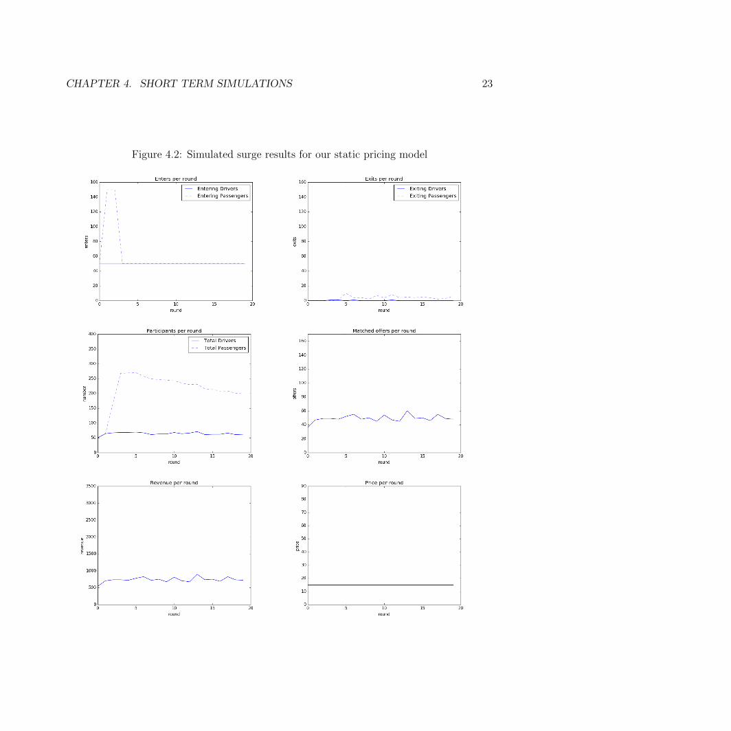
Static Pricing Results
We first used our static pricing model in our surge simulation. The results are shown inFigure 4.2.
Proportional Pricing Results
We experimented with two different approaches to proportional pricing: Uncapped vs.capped proportional pricing.
With uncapped proportional pricing, prices are directly proportional to the ratio of de-mand and supply. The problem with this approach is that whenever there is a sharp increasein demand, a sharp increase in price follows. However, this price can easily reach a pricethat no reasonable passenger would be willing to pay. We can already see this frustrationin real life, as passengers complain whenever Uber or Lyft enact any type of surge pricing.For example, Uber capped its surge pricing at 9.9x during the immensely busy New Year’sEve night in 2015. Rides that normally cost around $20 exceeded $100. This greatly hurtUber’s public image and business. To remedy this, in some areas, such as Boston, Uber hasput an artificial cap at 2.9x[21].
We emulate this cap in two ways. First, we experiment with setting a lower constant ofproportionality in our equation. By setting k as a lower value, we can limit the dynamic

CHAPTER 4. SHORT TERM SIMULATIONS 21
range of our price. The second method is to just set a cap on the pricing agent’s price. Inour case, we set the cap to be 2x the base price.
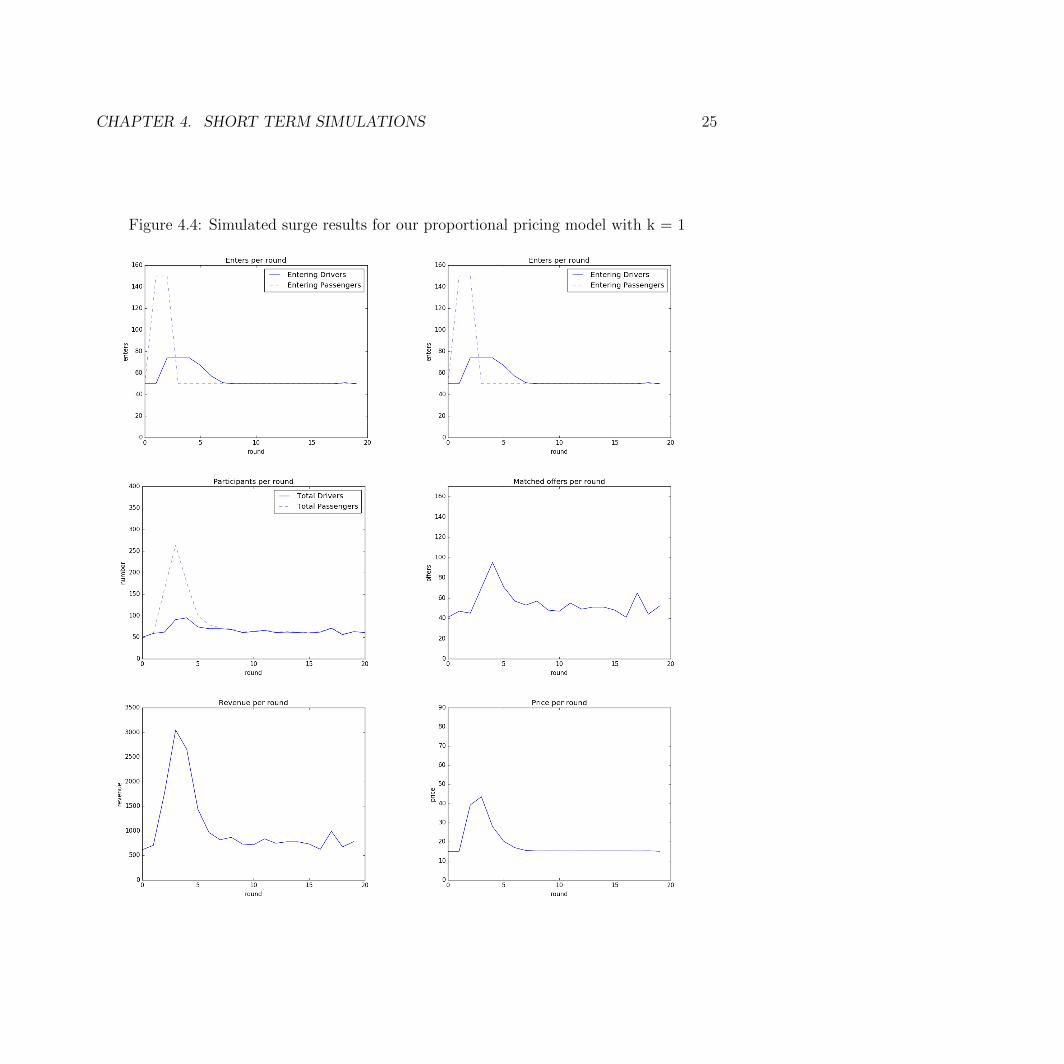
Results for uncapped proportional pricing with k=2 are shown in Figure 4.3. Resultsfor uncapped proportional pricing with k=1 are shown in Figure 4.4. Results for cappedproportional pricing are shown in figure 4.5.
Batch Update Pricing Results
For batch update pricing, we set the learning rate α to be 0.1. The results are shown inFigure 4.6.
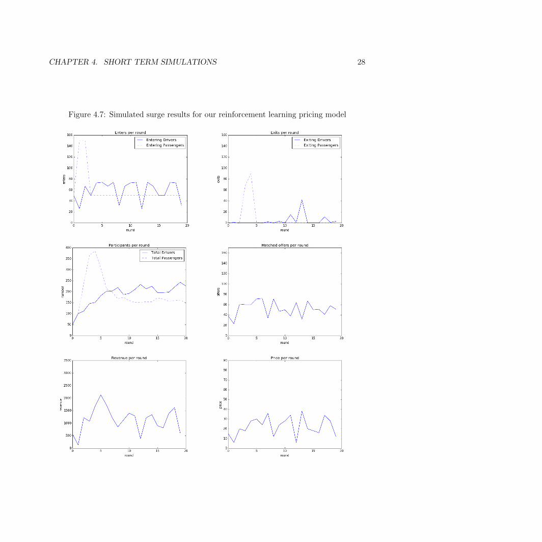
Reinforcement Learning Results
For reinforcement learning, we went through 50,000 iterations of training. In each iteration oftraining, the agent went through 20 rounds of the simulation. The results for reinforcementlearning pricing are shown in Figure 4.7.
4.3 Comparison
Results Overview
Pricing model Rt Ed Pm
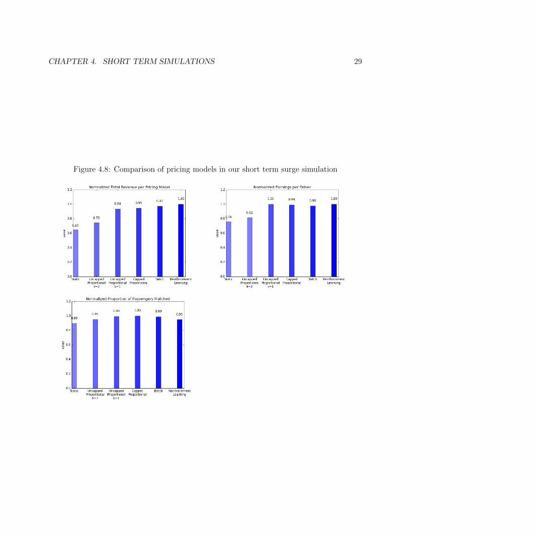
Static 0.65 0.76 0.90Proportional with k=1 0.75 0.82 0.95Proportional with k=2 0.94 1.00 0.99Proportional with cap at 2x 0.95 0.99 1.00Batch Update 0.97 0.98 0.99Reinforcement learning 1.00 1.00 0.95
Table 4.1: An overall comparison of pricing model performance for the short term simulation.Rt = normalized total revenue. Ed = normalized earnings per driver. Pm = normalizedproportion of passengers matched
Table 4.1 and Figure 4.8 show a comparison of all the pricing methods. In terms of totalrevenue, reinforcement learning outperforms all other pricing methods. We can observe afew important factors that seem to correlate to a pricing agent’s success in the surge pricingsimulation.
A phenomenon that we see is that there are many exiting passengers after the surge periodregardless of pricing model. These are all the passengers who were not matched due to thelack of drivers. It is obvious that there needs to be an increase in price when demand greatlyexceeds supply. With price sensitive drivers, increasing the price helps supply match demand.In simulations where the increase in drivers eventually matches the surge in passengers, there

CHAPTER 4. SHORT TERM SIMULATIONS 22
are a large amount of exiting drivers post-surge. This behavior is actually seen in real life.It is common for drivers to drive towards a surge area, but when they arrive, most of thepassengers have already left and the surge has ended, which causes dissatisfaction amongstdrivers.
The static pricing model is the only model that does not increase price in the surgesimulation. As a result, it does not take advantage of the increase in demand, because thenumber of matches is steady over time.
The simulations also show that drastic price increases are not a solution. In the uncappedproportional model, prices get as high as $100. As a result, no matches are made in thatround, because no passengers are willing to pay that high of a price. This also results in thelargest spike of exiting passengers.
The last three pricing models do not suffer from this problem. They respond to theincrease in demand, by raising prices to increase supply. As a result, the number of matchesincreases during the surge and revenue also spikes during the surge.
An interesting thing to note is that even though we did not put a price cap on the batchupdate and reinforcement learning pricing models, they both never exceed 3x the base price.In fact, the highest surge we see is the 2.5x in the RL model. This is similar to Uber’s surgecap of 2.9x in some areas of the United States[21].
Both batch update and RL pricing models reach similar revenue peaks after the surgeperiod. Total revenue for the RL model is higher because it tends to perform better onaverage at other times during the simulation. With more training, the RL model should beexpected to do even better as more state spaces are explored.
In terms of user and customer satisfaction, we can see that the RL model is amongthe highest in earnings per driver. However, the RL model is also the lowest in terms ofproportion of passengers that get matched. The sharp increases in prices that the RL modelmakes could be increasing profits at the expense of leaving some passengers unmatched.
From our short term simulation results, we can come to a few conclusions. If given thechoice, a company should implement the RL pricing model if they are only concerned aboutprofit maximization. The RL pricing model also comes with the benefit that on average,drivers are paid more. This results in long-term driver satisfaction and incentivizes drivers tojoin the platform. However, we can see that the RL model results in the lowest percentage ofpassengers that are eventually matched. This could be a problem if customers are sensitiveto inconsistent service. If RL prices lead to too many unhappy customers, this can lead tolow customer retention and poor public perception. Therefore, a company must determinewhether their cost-benefit analysis justifies sacrificing customer satisfaction for higher profitsand driver earnings. If not, another pricing model such as the batch update model might bemore optimal.
CHAPTER 4. SHORT TERM SIMULATIONS 23
Figure 4.2: Simulated surge results for our static pricing model

CHAPTER 4. SHORT TERM SIMULATIONS 24
Figure 4.3: Simulated surge results for our proportional pricing model with k = 2
CHAPTER 4. SHORT TERM SIMULATIONS 25
Figure 4.4: Simulated surge results for our proportional pricing model with k = 1

CHAPTER 4. SHORT TERM SIMULATIONS 26
Figure 4.5: Simulated surge results for our proportional pricing model with cap at 2x baseprice

CHAPTER 4. SHORT TERM SIMULATIONS 27
Figure 4.6: Simulated surge reactions to our batch update pricing model
CHAPTER 4. SHORT TERM SIMULATIONS 28
Figure 4.7: Simulated surge results for our reinforcement learning pricing model
CHAPTER 4. SHORT TERM SIMULATIONS 29
Figure 4.8: Comparison of pricing models in our short term surge simulation

30
Chapter 5
Long Term Simulations
5.1 Overview
For our long term simulations, each time step represents an hour. Our experiments last 720time steps, which is intended to simulate a month’s duration. Long term simulations areharder to simulate, since there additional factors that we are interested in keeping track of.We must now factor in acquisition and loss costs for both drivers and passengers. We didnot consider this in our short term simulations, because during the course of the day, bothcosts are negligible.
For customer acquisition, we initiate our simulation with an initial pool of 50 driversand passengers. We add a number drivers and passengers to our population each roundaccording to a normal distribution with mean 50 and standard deviation of 5. Each customeracquisition increases our cost by $20, and each driver acquisition increases our cost by $100.Our population is divided up into active and inactive agents. Each round, agents that areactive become inactive if they have not been matched for n rounds, where n is their roundtolerance. Agents that are inactive may become active with probability 0.5. Agents may alsopermanently leave the population. The probability that they permanently leave is related totheir satisfaction according to the probit distribution as mentioned in Chapter 2. Each timean active agent gets matched, their satisfaction increases by 0.1, and each time an activeagent does not get matched, their satisfaction decreases by 0.1. Therefore, if an agent isrepeatedly unmatched, they are more likely to defect permanently.
Our drivers also have a weekly income preference of $900, which equates to an hourlywage of $22.5. This means that each driver evaluates the amount of money they have madeover the past 140 rounds and sees whether or not their income has reached $45. If not, theyleave our system permanently. Depending on the market price, this means that drivers willhave be matched at least 3 to 4 times over the course of 7 rounds. For this simulation, weset the base market price as $15. The preferred price for both drivers and passengers is $15.Both drivers and passengers have a round tolerance of 2.

CHAPTER 5. LONG TERM SIMULATIONS 31
Static Pricing Results
We first used our static pricing model in our surge simulation. The results are shown inFigure 5.1. We can see that the price remains static throughout the whole simulation.Therefore, the pricing agent cannot use price to adjust supply to meet fluctuating demand.We can see a wide gap between active drivers and passengers. This cyclical gap is causedby unhappy passengers leaving because of the lack of drivers, which causes a driver surplus.This absence of passengers causes drivers to leave, which leads to a passenger surplus and arepeat of the whole process.
Proportional Pricing Results
We decided to set k=1 for our proportional pricing model. In order to calculate price, weonly considered the ratio between active passengers and drivers. The results are shown inFigure 5.2. We can see that proportional pricing does a great job of matching supply anddemand.
Batch Update Pricing Results
For batch update pricing, we set the learning rate α to be 0.1. The results for batch updatepricing are shown in Figure 5.3. Batch update pricing tends to maintain higher prices, whichcauses our simulation to have a high quantity of drivers at all times. There is a constantdriver surplus at all times during the simulation, which leads to high passenger match rates,but also higher driver dissatisfaction.
Reinforcement Learning Results
For reinforcement learning, we went through 50,000 iterations of training. In each iterationof training, the agent went through 720 rounds of the simulation. Results are shown inFigure 5.4. The results from reinforcement learning tend to be quite noisy. This is causedby the large fluctuations of pricing learned by the RL agent. RL pricing does a decentjob at matching driver and passenger quantities. Explanations for the large fluctuation inpricing could be that the pricing agent tends to take advantages of situations where it canprice higher to maximize profits. Then, it may make drastic decreases or increases in price toreduce the gap in supply and demand that might have resulted from its profit maximizations.
5.2 Comparison
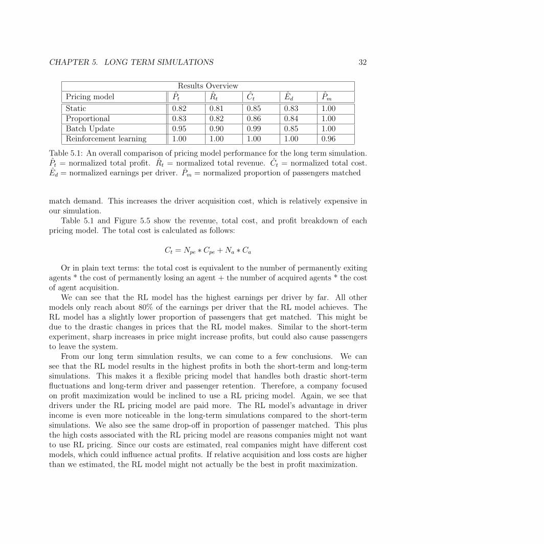
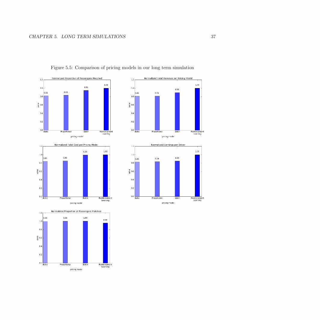
Table 5.1 and Figure 5.5 show a comparison of all the pricing methods. The RL model endsup with the highest profit and revenue out of all the models followed by the batch updatemodel, proportional model, and static model.
The proportional pricing model and the static pricing model tend to have higher costs.This cost is mostly due to the fact that both pricing models use prices to increase supply to
CHAPTER 5. LONG TERM SIMULATIONS 32
Results Overview
Pricing model Pt Rt Ct Ed Pm
Static 0.82 0.81 0.85 0.83 1.00Proportional 0.83 0.82 0.86 0.84 1.00Batch Update 0.95 0.90 0.99 0.85 1.00Reinforcement learning 1.00 1.00 1.00 1.00 0.96
Table 5.1: An overall comparison of pricing model performance for the long term simulation.Pt = normalized total profit. Rt = normalized total revenue. Ct = normalized total cost.Ed = normalized earnings per driver. Pm = normalized proportion of passengers matched
match demand. This increases the driver acquisition cost, which is relatively expensive inour simulation.
Table 5.1 and Figure 5.5 show the revenue, total cost, and profit breakdown of eachpricing model. The total cost is calculated as follows:
Ct = Npe ∗ Cpe +Na ∗ Ca
Or in plain text terms: the total cost is equivalent to the number of permanently exitingagents * the cost of permanently losing an agent + the number of acquired agents * the costof agent acquisition.
We can see that the RL model has the highest earnings per driver by far. All othermodels only reach about 80% of the earnings per driver that the RL model achieves. TheRL model has a slightly lower proportion of passengers that get matched. This might bedue to the drastic changes in prices that the RL model makes. Similar to the short-termexperiment, sharp increases in price might increase profits, but could also cause passengersto leave the system.
From our long term simulation results, we can come to a few conclusions. We cansee that the RL model results in the highest profits in both the short-term and long-termsimulations. This makes it a flexible pricing model that handles both drastic short-termfluctuations and long-term driver and passenger retention. Therefore, a company focusedon profit maximization would be inclined to use a RL pricing model. Again, we see thatdrivers under the RL pricing model are paid more. The RL model’s advantage in driverincome is even more noticeable in the long-term simulations compared to the short-termsimulations. We also see the same drop-off in proportion of passenger matched. This plusthe high costs associated with the RL pricing model are reasons companies might not wantto use RL pricing. Since our costs are estimated, real companies might have different costmodels, which could influence actual profits. If relative acquisition and loss costs are higherthan we estimated, the RL model might not actually be the best in profit maximization.

CHAPTER 5. LONG TERM SIMULATIONS 33
Figure 5.1: Simulated long term results for our static pricing model

CHAPTER 5. LONG TERM SIMULATIONS 34
Figure 5.2: Simulated long term reactions to our proportional pricing model
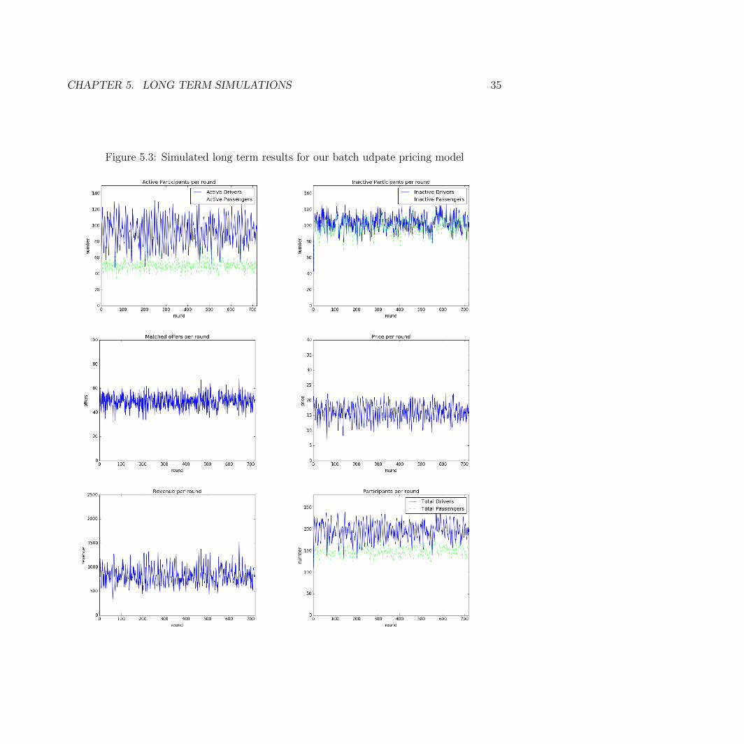
CHAPTER 5. LONG TERM SIMULATIONS 35
Figure 5.3: Simulated long term results for our batch udpate pricing model

CHAPTER 5. LONG TERM SIMULATIONS 36
Figure 5.4: Simulated long term results for our reinforcement learning pricing model
CHAPTER 5. LONG TERM SIMULATIONS 37
Figure 5.5: Comparison of pricing models in our long term simulation

38
Chapter 6
Future Work
Building a More Robust Simulation
The simulation we are currently using is quite simple. The state space is small in a sensethat it is only a combination of number of passengers, number of drivers, and price. Themain limitation is that it has no geographical data and can only model one lane. We canadd geographical data for each driver and passenger agent in the simulation. This wouldallow us the simulation to model lanes and agents in a geographical area.
The pain-point for adding geographical data is that we have to add location into thestate space and our agent preference models. For each agent, their preferences will nowdepend on their location relative to the lane location and the location of the other relevantagents in the environment. In addition, adding geographical data results in a huge statespace. However, we have known methods to deal with large state spaces, such as functionapproximation. We can use either a linear combination of state features or a neural networkas good function approximators for this problem. We could also approximate lane similarityby using the cosine distance between two lane vectors.
Inverse Reinforcement Learning
In our current simulation, we are simulating agent preferences based on market research andwhat we intuitively think how humans should act. However, if we are able to obtain a largedataset of real market data, we can apply inverse reinforcement learning techniques to learnactual agent preferences. With these learned preferences, our simulated agents should beable to act more similarly to real people.
Multi-Competitor Landscape
Currently we model losing an agent as a fixed cost per agent lost. It would be interestingto see how our pricing agent acts in the presence of other competitors in the marketplace.A simple way of simulating this would be to pit two or more of our pricing agents against

CHAPTER 6. FUTURE WORK 39
each other in the same simulation and see how they react. We might be able to see moreinteresting behaviour and tactics surrounding agent retention.
Modeling Natural Growth
One factor we have not modeled is natural growth of our agent population. We only consideractive customer acquisition in our current simulation. This creates a pessimistic predictionof customer and user growth. In real life, our agent population may grow due to word ofmouth, peer recommendations, and natural discovery. These growth factors need additionalmarket research before we can determine how to accurately apply them to the simulation.
Real-World Application
At the time of writing this paper, I am working as the cofounder of Dray TechnologiesInc. Dray is an online and mobile marketplace for the on-demand trucking industry. Thesimulation created here can be easily applied to the spot brokering aspect of trucking. Iplan to apply the reinforcement learning techniques used in this paper to generate instantprices for Dray’s trucking shipments. We can also use real market data obtained from ourshipments to create better simulations. It will be interesting to see how an automated agent’spredicted prices compare to marketplace rates.

40
Chapter 7
Conclusion
In this paper, we built a simulation that models agent behaviour in an on-demand market-place. We experimented with different pricing models in both short and long term simu-lations. We have shown that using reinforcement learning is an applicable solution to thisproblem. Overall, our reinforcement learning agent does the best job with regards to rev-enue and profit maximization. It beats out other pricing agents in both short term andlong term simulations. The RL agent also performs the best when factoring in earnings perdriver. However, the RL agent seems to maximize profits at the expense of ensuring matchesfor passengers. With these results in mind, a reinforcement learning agent can easily beexpanded to more complex state spaces and simulations.
The main motivation of writing this paper is to explore and better understand the pricingproblems that many on-demand companies face today. It is no longer sufficient to justforecast market uncertainties, because companies need a way to react to changes in real-time.An automated pricing agent is able to ingest data with scale and frequency while maximizingprofits without human supervision. In practice, a company using a reinforcement learningautomated pricing agent would be able to streamline its operations and improve its bottomline while retaining drivers and riders.

41
Bibliography
[1] 2010-2013 New York City Taxi Data. 2016. url: https://publish.illinois.edu/dbwork/open-data/.
[2] Lantseva et al. “Data-driven Modeling of Airlines Pricing”. In: Procedia ComputerScience 66 (2015), pp. 267–276.
[3] Malighetti et al. “Pricing strategies of low-cost airlines: The Ryanair case study”. In:Journal of Air Transport Management 145 (2009), pp. 195–203.
[4] Raju et al. “Reinforcement Learning Applications in Dynamic Pricing of Retail Mar-kets”. In: E-Commerce, 2003. CEC 2003. IEEE International Conference on (2003).
[5] Sousa et al. “Urban Logistics Integrated in a Multimodal Mobility System”. In: IEEEIntelligent Transportation Systems (2015).
[6] Yossi Aviv and Amit Pazgal. “A partially observed Markov decision process for dy-namic pricing”. In: Journal of Consumer Research 51 (9 2005), pp. 1400–1416.
[7] Dimitris Bertsimas and Georgia Perakis. “Dynamic Pricing; A Learning Approach”.In: Mathematical and computational models for congestion charging (2006), pp. 45–79.
[8] Ruth N Bolton. “A dynamic model of the duration of the customer’s relationship witha continuous service provider: The role of satisfaction”. In: Marketing science 17 (11998), pp. 25–26.
[9] Martin. Christopher. “The Agile Supply Chain: Competing in Volatile Markets”. In:Industrial Marketing Management 29 (2000), pp. 37–44.
[10] Pascal Courty. “Pricing Challenges in the Live Events industry: A Tale of Two Indus-tries”. In: IMC Roosevelt University (2015).
[11] Joan Morris DiMicco, Pattie Maes, and Amy Greenwald. “Learning curve: A simulation-based approach to dynamic pricing”. In: Electronic Commerce Research 3 (3 2003),pp. 245–276.
[12] Disney Introduces Demand-Based Pricing at Theme Parks. 2016. url: http://www.nytimes.com/2016/02/28/business/disney-introduces-demand-based-pricing-
at-theme-parks.html (visited on 02/27/2016).

BIBLIOGRAPHY 42
[13] Benjamin Edelman Edelman, Michael Ostrovsky, and Michael Schwarz. “Internet Ad-vertising and the Generalized Second Price Auction: Selling Billions of Dollars Worthof Keywords”. In: American Economic Review, American Economic Association 97(2001), pp. 242–259.
[14] Eyal Even-Dar and Yishay Mansour. “Learning Rates for Q-learning”. In: Journal ofMachine Learning Research 5 (2003), pp. 1–25.
[15] Marshall Fisher et al. “Making Supply Meet Demand”. In: Harvard Business Review(2015).
[16] Gallego Guillermo and Garrett Van Ryzin. “Optimal dynamic pricing of inventorieswith stochastic demand over finite horizons”. In: Management science 40 (8 1994),999=1020.
[17] Jonathan Hall, Cory Kendrick, and Chris Nosko. “The Effects of Ubers Surge Pricing:A Case Study”. In: The University of Chicago Booth School of Business (2015).
[18] Kelly L. Haws and William O. Bearden. “Dynamic pricing and consumer fairnessperceptions”. In: Journal of Consumer Research 33 (3 2006), pp. 304–311.
[19] Anton Leendert Hempenius. “Monopoly with random demand”. In: Rotterdam Uni-versity Press (1970).
[20] Justin Hienz. “Defining the Data Movement”. In: The Future of Data-Driven Innova-tion (2015).
[21] How Uber Chooses Its Surge Price Cap in Emergencies. 2016. url: http://abcnews.go.com/Business/uber- chooses- surge- price- cap- emergencies/story?id=
28494303.
[22] Junling Hu and Michael P. Wellman. “Multiagent reinforcement learning: theoreticalframework and an algorithm”. In: ICML 98 (1998).
[23] Zhu Ji and KJ Ray Liu. “Multi-stage pricing game for collusion-resistant dynamic spec-trum allocation”. In: Selected Areas in Communications, IEEE Journal 26 (1 2008),pp. 182–191.
[24] Jeffrey O Kephart, James E. Hanson, and Amy R. “Dynamic pricing by softwareagents”. In: Computer Networks 32 (6 2000), pp. 721–752.
[25] Jordan Kobritz and Steven Palmer. “Dynamic Pricing: The Next Frontier in the Evo-lution of Ticket Pricing in Sports”. In: International Handbook of Academic Researchand Training 10 (2010).
[26] Lyft SF Driver Bonus. 2016. url: www.lyft.com/SFBonus.
[27] Aranyak Mehta et al. “AdWords and generalized online matching”. In: Journal of theACM (2007), p. 22.
[28] NY Taxicab Rate of Fare. 2016. url: http : / / www . nyc . gov / html / tlc / html /
passenger/taxicab_rate.shtml (visited on 03/30/2016).

BIBLIOGRAPHY 43
[29] Edwin Pednault, Naoki Abe Abe, and Bianca Zadrozny. “Sequential Cost-SensitiveDecision Making with Reinforcement Learning”. In: Proceedings of the eighth ACMSIGKDD international conference on Knowledge discovery and data mining (2002).
[30] C. V. L. Raju, Y. Narahari, and K. Ravikumar. “Learning dynamic prices in electronicretail markets with customer segmentation”. In: Annals of Operations Research 143 (12006), pp. 59–75.
[31] Jimmy Ssu-Ging Shih. “Applying Congestion Pricing at Access Points for Voice andData Traffic”. PhD thesis. EECS Department, University of California, Berkeley, 2003.url: http://www.eecs.berkeley.edu/Pubs/TechRpts/2003/5572.html.
[32] Terry Taylor. “On-Demand Service Platforms”. In: Social Science Research Network(2016).
[33] Gunnar T Thowsen. “A dynamic, nonstationary inventory problem for a price/quantitysetting firms”. In: Naval Research Logistics Quarterly 22 (3 1975), pp. 461–476.
[34] Uber Promo. 2016. url: https://www.uber.com/promo/.
[35] A. S. De Vany and T. R. Saving. “The Effects of Ubers Surge Pricing: A Case Study”.In: The American Economic Review 67 (2015), pp. 583–594.
[36] Edward Zabel. “Multiperiod monopoly under uncertainty”. In: Journal of EconomicTheory 5 (3 1972), pp. 524–536.


![Automated Map Generation for the Physical Travelling ...julian.togelius.com/Perez2013Automated.pdf · Strategy (CMA-ES) [8], to automatically generate content by simulating agents](https://img.dokumen.tips/doc/110x75/5fb6dbce5f52490d423c1030/automated-map-generation-for-the-physical-travelling-strategy-cma-es-8.jpg)


