Embed Size (px)
Citation preview
AUTOMATED FARM FIELD
DELINEATION AND CROP ROW
DETECTION FROM SATELLITE
IMAGES
MELKAMU MESERET ALEMU
February, 2016
SUPERVISORS:
Dr. Valentyn Tolpekin
Dr.Ir. Wietske Bijker


Thesis submitted to the Faculty of Geo-Information Science and Earth
Observation of the University of Twente in partial fulfilment of the
requirements for the degree of Master of Science in Geo-information Science
and Earth Observation.
Specialization: Geoinformatics
SUPERVISORS:
Dr. Valentyn Tolpekin
Dr.Ir. Wietske Bijker
THESIS ASSESSMENT BOARD:
Prof.Dr.Ir. A. Stein (Chair)
Dr. I.C. van Duren (External Examiner, University of Twente, ITC-NRS)
AUTOMATED FARM FIELD
DELINEATION AND CROP ROW
DETECTION FROM SATELLITE
IMAGES
MELKAMU MESERET ALEMU
Enschede, The Netherlands, February, 2016

DISCLAIMER
This document describes work undertaken as part of a programme of study at the Faculty of Geo-Information Science and
Earth Observation of the University of Twente. All views and opinions expressed therein remain the sole responsibility of the
author, and do not necessarily represent those of the Faculty.

i
ABSTRACT
Agriculture is vital to the food security and economic growth of most countries in the world, especially in
developing countries. Accurate information on field boundaries has considerable importance in precision
agriculture and greatly assists land administration systems. The information obtained from field
boundaries can provide valuable input for agricultural applications like crop monitoring and yield
predictions.
Farm field information extraction is an important task and is highly related to food security. Farm field
boundaries can be delineated by conventional field surveying methods or by digitizing satellite imagery
manually. However, this approach is time consuming, costly and highly dependent on the operator‟s
capability of digitization and interpretation. Low and medium resolution satellite images have limited
capacity to offer accurate information for field level. But, very high resolution satellite images can provide
farm field information accurately to sub-meter level, though extracting the required information from
them is a big challenge due to the complex ground environment.
In this research, the capability of the line segment detection (LSD) algorithm for extracting linear features
is explored on two real applications in the agricultural sector: field boundary delineation and crop rows
detection from very high resolution satellite images. The algorithm starts by calculating the level-line angle
for each pixel based on pixel gradient As LSD is taking only a single band as an input, in order to
concentrate all the available information, the gradient information in all bands is combined as a single
band by taking the vector sum of image gradients in all bands. The level-line angle is used to form the
line-support region, potential candidates for a segment, and is validated by Helmholtz principle based on
NFA calculation. In addition to image bands, texture bands were explored. The effects of different second
order GLCM texture measures on the results of LSD were examined.
In this research, validation method was developed The optimum values of the three internal parameters of
LSD for the purpose of field boundary delineation were S = 1.0, and Similarly, the
optimum values these parameters for crop rows detection were S = 0.8, τ=22.5° and ε =1.0. These
optimum parameter values agree with the ones proposed by Grompone von Gioi et al. (2012) except
some difference on the scale parameter for the first application.
Accuracy assessment was performed following the proposed method by defining the two error ratios: the
ratio of missing detection and the ratio false detection. The results obtained for the first application (field
boundary delineation) are RM=0.78 and RF= 0.73. The results for the second application (crop rows
detection) are RM =0.17 and RF=0.48.
In this research, the different approaches followed: extracting information from multiple bands, using
texture bands or image bands in detecting field boundaries do not give good results. On the other hand,
the results obtained from the crop rows detection show that the adopted methodology has a good
potential in detecting crop rows as well as their dominant orientations.

ii
ACKNOWLEDGEMENTS
I would like to express my heartfelt appreciation to my supervisors Dr. Valentyn Tolpekin and
Dr.Ir.Wietske Bijker for their continued support, guidance, encouragement, immense knowledge and for
their patience. I have indeed learnt a lot from them.
I sincerely thank Dafni Sidiropoulou Velidou for allowing me to use part of the LSD R code.
I am also grateful to all Staff members of ITC who in one way or another involved in my learning process
and to the Netherlands Fellowship Programmes (NFP) for awarding me the scholarship that made my
studies possible at ITC.
I would like to thank my family for their love, steady encouragement and support. To my brother
Workineh Meseret and sisters Desta and Mahlet Meseret thank you for everything. To Yenework
Mulualem I have no words to say but thank you for your patience and understanding.
Lastly, I heartily thank all Habesha community at ITC for making my stay at ITC enjoyable and
memorable.
Melkamu Meseret Alemu February, 2016

iii
TABLE OF CONTENTS
Abstract ............................................................................................................................................................................ i
Acknowledgements ....................................................................................................................................................... ii
List of figures ................................................................................................................................................................. v
List of tables .................................................................................................................................................................vii
1. Introduction ........................................................................................................................................................... 1
1.1. Problem statement ......................................................................................................................................................1 1.2. Background ...................................................................................................................................................................3 1.3. Research Identification ...............................................................................................................................................4
1.3.1. Research Objective ................................................................................................................................... 4
1.3.2. Research Questions .................................................................................................................................. 4
1.4. Innovation aimed at ....................................................................................................................................................5 1.5. Method adopted...........................................................................................................................................................5 1.6. Outline of the thesis ....................................................................................................................................................7
2. Literature Review .................................................................................................................................................. 9
2.1. Boundary concepts ......................................................................................................................................................9 2.2. Gestalt theory and The Helmholtz principle .........................................................................................................9 2.3. Texture information for image segmentation and boundary mapping ........................................................... 10 2.4. Related works ............................................................................................................................................................ 10 2.5. Accuracy Assessment ............................................................................................................................................... 12
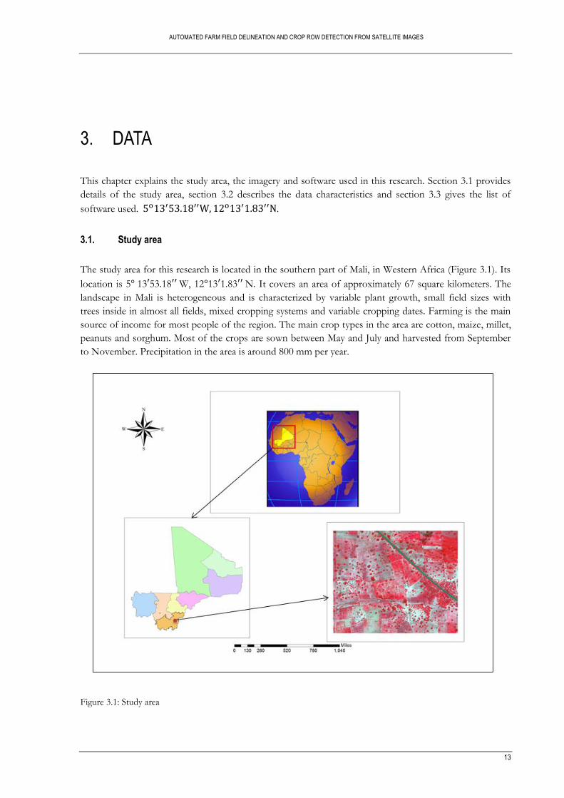
3. Data ...................................................................................................................................................................... 13
3.1. Study area ................................................................................................................................................................... 13 3.2. Imagery and Reference data ................................................................................................................................... 14
3.2.1. Very High Resolution Satellite image ................................................................................................. 14
3.2.2. Reference data ........................................................................................................................................ 14
3.3. Software ..................................................................................................................................................................... 14
4. Methodology ....................................................................................................................................................... 15
4.1. Texture calculation ................................................................................................................................................... 15
4.1.1. GLCM contrast ...................................................................................................................................... 16
4.1.2. GLCM dissimilarity ............................................................................................................................... 16
4.1.3. GLCM homogeneity ............................................................................................................................. 16
4.1.4. GLCM entropy ....................................................................................................................................... 16
4.1.5. GLCM angular second moment (ASM) and energy ........................................................................ 16
4.1.6. GLCM mean ........................................................................................................................................... 16
4.1.7. GLCM variance ...................................................................................................................................... 16
4.1.8. GLCM correlation ................................................................................................................................. 16
4.2. Line Segment Detection Algorithm ...................................................................................................................... 17
4.2.1. Multispectral analysis ............................................................................................................................. 18
4.2.2. Image scaling........................................................................................................................................... 18
4.2.3. Gradient computation ........................................................................................................................... 18
4.2.4. Gradient ordering and threshold ......................................................................................................... 20
4.2.5. Region Growing ..................................................................................................................................... 20
4.2.6. Line segment localization ..................................................................................................................... 21
4.2.7. Rectangular approximation .................................................................................................................. 22
4.2.8. Number of False Alarms (NFA) computation .................................................................................. 23

iv
4.3. Crop rows detection ................................................................................................................................................. 24 4.4. Parameter tuning and validation ............................................................................................................................ 25
4.4.1. Edge Strength Determination ............................................................................................................... 25
4.4.2. Validation and Accuracy Assessment ................................................................................................. 27
4.4.3. Parameter tuning ..................................................................................................................................... 28
5. Results .................................................................................................................................................................. 29
5.1. Farm field delineation .............................................................................................................................................. 29
5.1.1. Tuning of S .............................................................................................................................................. 29
5.1.2. Tuning of gradient magnitude threshold ........................................................................................ 32
5.1.3. Tuning of angle tolerance ...................................................................................................................... 33
5.1.4. Tuning of detection threshold epsilon ( ......................................................................................... 35
5.2. Parameter tuning for crop rows detection ........................................................................................................... 39
5.2.1. Tuning of S .............................................................................................................................................. 39
5.2.2. Tuning of .............................................................................................................................................. 42
5.2.3. Tuning of detection threshold .......................................................................................................... 43
5.3. Validation of the results of crop rows detection ................................................................................................ 45 5.4. Dominant orientation of crop rows ..................................................................................................................... 48 5.5. Spacing of Crop rows .............................................................................................................................................. 50
6. Discussion ............................................................................................................................................................ 51
6.1. Field boundary delineation ..................................................................................................................................... 51 6.2. Crop rows detection ................................................................................................................................................. 52
7. Conclusions and recommendations................................................................................................................. 53
7.1. Optimal parameter setting ...................................................................................................................................... 53 7.2. Assessment of the detection results ...................................................................................................................... 53
7.2.1. Field boundary delineation .................................................................................................................... 53
7.2.2. Crop rows detection ............................................................................................................................... 53
7.3. Recommendations .................................................................................................................................................... 54
List of references ......................................................................................................................................................... 55
Appendix ...................................................................................................................................................................... 60

v
LIST OF FIGURES
Figure 1.1: Flowchart of the methodology ................................................................................................................ 6
Figure 3.1: Study area ................................................................................................................................................. 13
Figure 4.1: The four directions for calculating texture features. ......................................................................... 15
Figure 4.2: (a) Example of input image with 4 grey levels (b) GLC M for distance d =1 and direction 0°. 15
Figure 4.3: Gradient computation using 2×2 mask. ............................................................................................. 19
Figure 4.4: Image gradient. (a) Horizontal direction, (b) Vertical direction ...................................................... 19
Figure 4.5: Edge orientation, reprinted from Meer and Georgescu (2001) ...................................................... 20
Figure 4.6: Regional growing process of aligned points, reprinted from Morel et al. (2010) ......................... 21
Figure 4.7: Representation of a line by and θ. .................................................................................................... 22
Figure 4.8: Example of a line-support region and its associated line segment. ................................................ 22
Figure 4.9: The smallest rectangle that covers all pixels of the line-support region: (a) without line segment.
(b) with line segment .................................................................................................................................................. 23
Figure 4.10: Rotating the lines by angle to make them parallel to the x-axis, d is the spacing between the
lines. .............................................................................................................................................................................. 24
Figure 4.11: Line- support region W with its corresponding line that divides the region into and . 25
Figure 4.12: Steps in edge strength determination. ............................................................................................... 26
Figure 5.1(a) Ratio of missing(RM) and ratio of false (RF) detections, (b) RM+RF for varying scale
parameter S for fixed =22.5° and =1. The low S value would imply coarse spatial resolution and large
S value would imply fine spatial resolution. ........................................................................................................... 30
Figure 5.2: Detection results for different S values. (a) S = 0.2 , (b) S = 0.5 , (c) S = 0.8, (d) S = 1.0. Blue
segments: reference segments, white: detected segments. For the image displayed: R= 7, G = 5, B = 3. .. 30
Figure 5.3: Distance between points for varying the value of S ....................................................................... 31
Figure 5.4: Box plots showing distributions of contrast and steepness of true detections and false
detections. (a) Contrast of successful detections, ( b) Contrast of false detections, (c) Steepness of true
detections, (d) Steepness of false detections. ......................................................................................................... 32
Figure 5.5 (a) Ratio of missing (RM) and ratio of false (RF) detections, (b) RM+RF for varying for
fixed S = 1.0 and =1.0. ........................................................................................................................................... 33
Figure 5.6: Detection results for different values for fixed values .0 (a) , (b)
, (c) , (d) . Blue segments are reference segments, white segments are
detected segments. For image displayed R=7, G=5, B=3. ................................................................................. 34
Figure 5.7: Detected line segments with reference dataset on image band( blue segments are reference
segments, white segments are detected segments, R=7, G=5, B=3) for S=1, τ=22.5° and ε=1. ................. 36
Figure 5.8: Successful detections from reference to detection for S=1, Blue segments
are reference segments, black segments are detected segments, green segments show successful detections.
....................................................................................................................................................................................... 36
Figure 5.9: Successful detections from detection to reference for S=1, τ=22. 5°, ε=1. Blue segments are
reference segments, red segments are detected segments, green segments show successful detections. ..... 37
Figure 5.10: RM and RF for three spatial distance values in the horizontal direction. (a) GLCM contrast,
(b) GLCM mean, (c) GLCM variance. ................................................................................................................... 38
Figure 5.11: Detected line segments with reference dataset on texture band (GLCM contrast for in
the horizontal direction) for S=1, Blue segments are reference segments, white
segments are detected segments, R=7, G=5, B=3. .............................................................................................. 38

vi
Figure 5.12 (a) Ratio of missing(RM) and ratio of false(RF) detections, (b) RM+RF for varying scale
parameter S for fixed and . The low S value would imply coarse spatial resolution and
large S value would imply fine spatial resolution. An optimum value is observed at S = 0.8......................... 40
Figure 5.13: Successful detections for two different S values. Green: successful detection. (a) Successful
detections from reference to detection for S =0.5, (b) Successful detections from detection to reference
for S =0.5, (c) Successful detections from reference to detection for S =0.8, (d) Successful detections from
detection to reference for S =0.8. Detection results are better for (c) and (d) than (a) and (b). which shows
the influence of scale parameter on detection results............................................................................................ 41
Figure 5.14: (a) Ratio of missing(RM) and ratio of false(RF) detections, (b) RM+RF for varying angle
tolerance . Low values are more restrictive for region growing, which does not allow pixels with large
differences in gradient orientation to be included in the same line-support region. ........................................ 42
Figure 5.15: Detected results for optimum parameter values S=0.8, and . ......................... 43
Figure 5.16: Successful detections from reference to detection for optimum parameter values S=0.8,
=22.5° and =1. Green color shows successful detections, red color shows missed detections, black
lines are detected rows. ............................................................................................................................................... 44
Figure 5.17: Successful detections from detection to reference for optimum parameter values S = 0.8,
and . Green line segments show successful detections, red line segments show false
detections. ..................................................................................................................................................................... 44
Figure 5.18: Results of Subset 1 for optimum parameter values S=0.8, τ=22.5° and ε=1. (a) Detected
results, (b) Successful detections from reference to detection, (c) Successful detections from detection to
reference........................................................................................................................................................................ 46
Figure 5.19: Results of Subset 4 for optimum parameter values S=0.8, τ=22.5° and ε=1. (a) Detected
results, (b) Successful detections from reference to detection, (c) Successful detections from detection to
reference . ..................................................................................................................................................................... 47
Figure 5.20: Detected results for optimum parameter values S=0.8, τ=22.5° and ε=1 of a field with no
crop rows. No detection was reported in the field except near the boundaries of the field. .......................... 48
Figure 5.21: Rose diagram of dominant orientation of crop rows of both reference and detection for four
validation subsets. (a-d) are the orientations of reference rows and (e-h) are the orientations of their
corresponding detected rows of subsets 1-4 respectively. .................................................................................... 49
Figure 5.22: Row spacing of four subsets. (a) Subset 1, (b) tuning subset, (c) subset 3, (d) subset 4. The
vertical lines indicate the lags at which dominant frequencies are found. ......................................................... 50

vii
LIST OF TABLES
Table 3.1: WorldView-2 satellite image specifications. ......................................................................................... 14
Table 5.1: RM and RF for varying S for fixed and . .............................................................. 29
Table 5.2: RM and RF for varying gradient magnitude threshold for fixed S =1, =22.5° and =1. ....... 32
Table 5.3: RM, RF, Average distance and standard deviation between corresponding points for varying τ
for fixed S=1. 0 and ε=1. .......................................................................................................................................... 33
Table 5.4: RM and RF for varying detection threshold for fixed S = 1.0 and 22.5 . ........................... 35
Table 5.5: RM and RF for three spatial distance values ....................................................................................... 37
Table 5.6: RM and RF for varying S for fixed and . ............................................................... 39
Table 5.7: RM and RF for varying angle tolerance and for fixed values of S=0.8 and 1. ................... 42
Table 5.8: RM and RF for varying detection threshold and for fixed values of S=0.8 and 22.5 . ..... 43
Table 5.9: RM and RF for different subsets for optimum parameter values S = 0.8, and .
....................................................................................................................................................................................... 45
Table 5.10: Dominant orientation of crop rows and number of rows .............................................................. 48
Table 5.11: Spacing of crop rows for four subsets. ............................................................................................... 50


AUTOMATED FARM FIELD DELINEATION AND CROP ROW DETECTION FROM SATELLITE IMAGES
1
1. INTRODUCTION
1.1. Problem statement
Agriculture is vital to the food security and economic growth of most countries in the world, especially in
developing countries. African economies depend heavily on agriculture and the agriculture provides a large
share of the gross domestic product (GDP) in some sub-Saharan African countries (AGRA, 2013). Most
farming in Africa is carried out by smallholders using traditional techniques. These smallholders contribute
up to 90% of the nations‟ staple food production (Jain et al., 2013) by using traditional farming practices.
They do not have access to modern agriculture knowledge and techniques. Though agriculture contributes
a large share to GDP, most African countries are self-insufficient in food. Alleviating food insecurity and
ensuring sustainable development in the region is one of the top agenda that seeks attention. Proper
management of land resources is the basis for sustainable development and is directly related to
agricultural development and food security (Dekker, 2001). To manage land resources effectively, there is
a need for reliable, accurate and up to date information system about land. The main aim of land
administration systems is to improve tenure security and access to land (Lengoiboni et al., 2011).
However, land administration systems and proper management policies remain a challenge to most
African countries (Kurwakumire, 2014). Depending on development stage of the economy and land
tenure (mode of holding or occupying land) arrangements, land administration faces many challenges
(Bogaerts & Zevenbergen, 2001). The lack of transparent land tenure information systems severely limits
the engagement of smallholders, communities and investors in sustainable investment in land resources
and generates social instability through land disputes. Tenure security provides community and investor
confidence in development planning, land-based economic growth, natural resource management and
environment sustainability and social stability (Donnelly, 2012). The core of land administration and
tenure security is agreements on location of property boundaries. The interpretation of the location of
these boundaries can be difficult and judgments may vary depending on the interpretation of the evidence
of the location (Donnelly, 2012). Accurate information on field boundary has considerable importance in
precision agriculture and greatly assists land administration systems. Therefore, it is important to find
affordable technologies and efficient methods that assist decision making and effective use of land
resources. Modern technologies, such as remote sensing and spatial information systems are
revolutionizing agriculture. However, the use of these technologies is still far in Africa due to the
heterogeneous nature of the agriculture, differences in crop cycles, the spatial heterogeneity of landscape,
small and ill-defined farm fields, data accessibility issues, especially for high resolution data. This challenge
has a negative impact on the proper planning, monitoring and effective utilization of land resources for
sustainable development of the region. Thus, research based agricultural innovations, high precision and
low cost technologies and suitable information extraction methods that can be easily applied in the region
are essential to overcome challenges. To this end, The Spurring a Transformation for Agriculture through
Remote Sensing (STARS) project, a research project looking for ways how remote sensing technology can
help to improve agricultural practices and advance the livelihoods of smallholder in Sub-Saharan Africa
and South Asia, is working to overcome the barriers and challenges of agricultural practices and land
management related issues by finding evidence-based solutions sustainably so that smallholders, the
farming community and decision makers can benefit out of it.

AUTOMATED FARM FIELD DELINEATION AND CROP ROW DETECTION FROM SATELLITE IMAGES
2
Agricultural applications (like crop row identification, crop protection and yield estimation) of remote
sensing technology require quantitative analysis of remotely sensed data with high accuracy and reliability
(Ferencz et al., 2004) and these can be achieved better on a field level. But, the definitions of the the
words „field‟ and „boundary‟ are context dependent. So, the fundamental unit of land that shares a certain
property (parcel) need to be defined and identified. The parcel is described by its boundaries. Delineation
of farm field boundaries is an important task to provide reliable information for monitoring farm fields
and for yield prediction. Such predictions are crucial for field-level planning and site specific
recommendations. Many information extraction techniques (surveys) have been used to delineate field
boundaries. Generally, these methods can be grouped into three parts: ground based surveying, aerial
surveys and satellite based surveying (Ali et al., 2012). Ground based surveying methods are conducted by
surveyors using different surveying techniques and instruments like optical square, plane tabling etc.
Nowadays, Global Positioning System (GPS) is broadly used to locate the position of points on the
ground. Ground based survey is quite accurate, but labor intensive, sometimes requires an enormous
amount of time and resources, including a number of skilled surveyors for large area application. On the
other hand, aerial survey from aerial photogrammetry offers cost effective and time saving means of
information extraction for land surveying and mapping. Moreover, aerial survey offers richer data than
ground survey vector data (Barry & Coakley, 2013). Although the aerial survey is a better alternative to
ground based survey, it is highly dependent on weather and climatic conditions (Ali et al., 2012).
Sometimes, it is also impossible to undertake aerial surveys in some regions due restrictions for military
security reasons. Satellite based surveying is the other method which offers many of the required spatial
inputs for land surveying in digital form. As compared to aerial surveying, satellite based surveying covers
a wide area more repeatedly and economically (Ali et al., 2012). Moreover, because of increasing spatial
resolution satellite imagery is becoming more and more a viable alternative to aerial photographs.
Linear features extracted from remotely sensed data are important data sources for geospatial information
analysis. Edges in the remote sensing image describe the structural information of linear ground objects
such as field boundaries and crop rows. Thus, linear feature extractgion( edge detection) is an important
task for boundary delineation and crop row detection.
Over the years, many methods have been proposed to delineate field boundaries using semi-automatic and
automatic methods (Ji, 1996), (Reyberg et al., 2001), (Torre & Radeva, 2000), (Turker & Kok, 2013).
Standard edge detection methods work reasonably well in Western Europe and North America. But these
methods fail to detect field boundaries in the study area Mali (STARS project, personal communication).
The main problems are vague field boundaries and spatial heterogeneity of the regions on the both sides
of the boundary.
Low and medium resolution satellite images have limited capacity to offer accurate information for field
level. Moreover, they are not suitable for crop rows detection due to the small size of the elements to
detect. On the other hand, very high resolution satellite images contain rich and detailed ground
information, and they can reflect farm field information accurately to sub-meter level. But due to the
complex ground environment, extracting the required information from very high resolution satellite
images is a big challenge. Therefore, it is of importance to develop methodology that facilitates automatic
extraction of linear features (edges) that represent field boundaries and crop rows from very high
resolution satellite imagery.

AUTOMATED FARM FIELD DELINEATION AND CROP ROW DETECTION FROM SATELLITE IMAGES
3
1.2. Background
This part gives background knowledge on different edge detection techniques including line segment
detector. It also gives a general idea about image segmentation and related concepts like texture.
Edge detection
An edge is a part of the image where the brightness of the image changes abruptly. Edge detection is a
process of detecting and locating sharp discontinuities in the grey values of an image (Ziou & Tabbone,
1998). Many edge detection methods have been developed. The performance of an edge detection
operator highly depends on lighting conditions and noise (Bhardwaj & Mittal, 2012). Most edge detection
algorithms work well only in the images with sharp intensity transitions. They are also sensitive to noise.
For this reason, smoothing operation is required to reduce noise in the image before the actual edge
detection. This smoothing has a negative effect as it distorts the edge information. To keep balance
between edge information and smoothing, the image is filtered with appropriate kernel such as Gaussian
kernel. Due to the presence of noise the operators extract false edges. The operators also fail to find the
boundaries of objects that have a small change in intensity values or change in intensity that occurs over a
long distance, that leads to both problems of detection and localization of edges (Bhardwaj & Mittal,
2012). Therefore, problems of false edge detection, missing edges and poor localization of edges limit the
applicability of the algorithms.
Recently, a number of edge detection methods based on Gestalt theory and Helmholtz principle were
presented. Gestalt theory describes the laws of human visual reconstruction and Helmholtz principle
states that noticeable structures may be viewed as exceptions to randomness (Tepper et al., 2014). Moisan
and Morel (2000) applied edge detection methods, without any a priori information, based on the Gestalt
theory and the Helmholtz principle. According to a basic principle of perception due to Helmholtz, an
observed geometric structure is “meaningful” if it has a low probability to appear in a randomly created
image (Desolneux et al., 2003). This is called “a contrario” approach. In this approach, instead of
characterizing the elements we wish to detect, on the contrary, we characterize the elements we wish to
avoid detecting. When an element sufficiently deviates from the background model, it is considered as
meaningful and hence, detected (Tepper et al., 2014). To any geometric event on an image there is number
of false alarms (NFA) associated to it. The NFA of an event is defined as the expectation of the number
of occurrences of the event in a pure noise image of the same size.
Line Segment Detector
Line segments provide expressive information about the geometric content of images. Many algorithms
have been developed and implemented to extract line segments from images. Hough Transform (HT) is
one well known method to detect lines from images (Nixon & Aguado, 2012). Other recent
implementation is a line segment detector (LSD) algorithm presented by Grompone von Gioi et al. (2012)
built on the method of Burns et al. (1986). It integrates line segment detection with the Helmholtz
principle. The LSD algorithm is currently developed to detect straight line segments from images. It is
only suitable to detect straight edges from images. Nevertheless, large parts of the edges (for example field
boundaries) are not really straight, but curved.
Image Segmentation
Image segmentation is a division of an image into multiple sub-regions based on a desired feature. There
are two main approaches to segment images: edge-based and region-based (Faruquzzaman et al., 2008).
Edge-based segmentation partitions the image into sub-regions by looking for discontinuities in image
intensity, whereas region-based segmentation methods partition the images into different sub-regions of
closed boundaries with the assumption that pixels in the same category have certain homogeneity in

AUTOMATED FARM FIELD DELINEATION AND CROP ROW DETECTION FROM SATELLITE IMAGES
4
spectral values (Evans et al., 2002). Region based segmentation may be classified as the bottom-up
approach which merges smaller region into larger ones, top-down approach which splits an image into
smaller regions and the mixed approach which leads to splitting and merging regions (Faruquzzaman et al.,
2008). There are several measures that are used to decide whether regions should be merged or split.
Texture measure is one of them.
Texture
Texture is an important spatial feature that is used for analysis and interpretation of digital images.
According to Haralick (1979), texture is defined as the spatial variation in image intensities. It describes
visual information that is related to local variation in orientation, color and intensity in an image (Min,
2015). Texture analysis requires the identification of important features that differentiate the textures in
the image for classification, segmentation and recognition (Arivazhagan & Ganesan, 2003). The gray level
co-occurrence matrix (GLCM), introduced by Haralick et al. (1973) as “gray-tone spatial-dependence
matrix”, shows different combinations of gray levels occurrence in an image. A number of statistical
texture features can be computed from GLCM. Statistics are classified as first order, second order or
higher order statistics depending on the number of pixels in each combination. Homogeneity, dissimilarity,
entropy, mean, standard deviation, contrast, energy and correlation are the most widely used second order
statistics in the remote sensing imagery analysis. The construction of gray-level co-occurrence matrix
depends on different parameters: the number of gray levels used in the matrix, the window size, the
distance and the orientation. There are also other simple statistical texture measures that use edge density
and direction to characterize the texture.
This research focuses on one specific topic on the larger STARS frame, that is, automated farm field
delineation and crop row detection from satellite images. Conventional edge detection methods have been
used for farm field boundary delineation. But, these methods are not efficient to detect field boundaries
when fields have complex landscapes. The LSD algorithm is currently developed to detect straight line
segments from images and is successful to automatically detect straight linear features from images.
Therefore, modifying the LSD algorithm and using its capability for boundary delineation and crop row
detection is an important task. The capabilities of very high resolution satellite imagery (both in spatial and
spectral) with appropriate methodology gave opportunity to investigate the above mentioned problem and
test in a test area in Mali.
1.3. Research Identification
1.3.1. Research Objective
The main objective of this research is to develop a procedure and implement image analysis methods to
adapt the line segment detection algorithm and make it applicable for farm field boundary delineation and
crop rows detection from very high resolution satellite imagery.
Research Sub- Objectives
1. To identify the influence of the internal parameters of the algorithm on the quality of the results.
2. To identify the appropriate band as an input for LSD algorithm.
3. To compare and select textural features characterizing farm fields from satellite images.
4. To accurately locate crop rows from satellite images.
5. To develop validation methods for evaluation of the result.
1.3.2. Research Questions
1. What are the optimal values of the parameters for the proposed applications?
2. How to incorporate multispectral information as an input to LSD algorithm?

AUTOMATED FARM FIELD DELINEATION AND CROP ROW DETECTION FROM SATELLITE IMAGES
5
3. Can texture help in the field boundary delineation? If so, which texture measure and distance in
GLCM processing are appropriate?
4. What is the dominant orientation of crop rows in a particular field?
5. How successful is LSD in detecting field boundaries and crop rows?
6. Do accuracy measures positional accuracy, correctness, completeness, false detection ratio and
missing detection ratio fit for a particular purpose?
1.4. Innovation aimed at
The novelty in this study is to adapt the line segment detector (LSD) algorithm and make it applicable for
automated agricultural farm field boundary delineation and crop row detection from satellite images.
1.5. Method adopted
The flow chart in Figure 1.1 shows an overview of the methodology followed to reach the objectives and
answer research questions. The detail process is further explained in Chapter 4.

AUTOMATED FARM FIELD DELINEATION AND CROP ROW DETECTION FROM SATELLITE IMAGES
6
Satellite
image
Region of
interest
Selecting Scale
parameter
Rectangle
approximation
Gradient
magnitude
Gradient
orientation
Gradient
orderingGradient
threshold
Region growingLine support
regionsNFA
Final rectangle
approximation
Gradient Computation
NFA Computation
Line segments
Add texture
layer
Accuracy
Assessment
Ground truth
Validation
Figure 1.1: Flowchart of the methodology

AUTOMATED FARM FIELD DELINEATION AND CROP ROW DETECTION FROM SATELLITE IMAGES
7
1.6. Outline of the thesis
Chapter 2 is a literature review on Boundary concepts, Gestalt theory and The Helmholtz Principle and
texture information for image segmentation.
Chapter 3 describes the study area and the data used in this research.
Chapter 4 presents the methodology applied in this research.
Chapter 5 discusses the results of the study.
Chapter 6 describes general discussions.
Chapter 7 gives summary of conclusions and recommendation.


AUTOMATED FARM FIELD DELINEATION AND CROP ROW DETECTION FROM SATELLITE IMAGES
9
2. LITERATURE REVIEW
2.1. Boundary concepts
Dale &McLaughlin (1988) define boundary in legal sense as “a vertical surface that defines where one land
owner‟s territory ends and the next begins.” Williamson et al. (2010) provided a comprehensive
definition of the term boundary as “either the physical objects that mark the limits of a parcel, property, or
interest in land or an imaginary line or surface making or defining the division between two legal interests
in land.” According to Oxford Dictionary, the words „field‟ and „boundary‟ are defined as: Field, “an area
of open land, especially one planted with crops or pasture, typically bounded by hedges or fences”.
Boundary, “line which marks the limits of an area; a dividing line.” A more specific definition of boundary
is the one given by Jing et al. (2011), boundary as an imaginary line that marks the bounds of two
adjoining parcels of land. There are two broad categories of boundaries: fixed boundaries and general
boundaries (Dale &McLaughlin, 1988). Fixed boundaries are boundaries that can be surveyed accurately
and expressed by bearings and distances, or by coordinates whereas general boundaries are boundaries
where the precise line of boundary between adjacent parcels has not been determined, but, it is usually
represented by either natural or man-made physical features like fences, hedges, roads etc. (Williamson et
al., 2010). Different rules of interpretation and definition of boundaries apply depending on the nature and
type of boundaries. Therefore, in this research field would be related to land use and crop type, whereas
boundaries would be related to edge features where changes in these types take place. A similar conclusion
is also drawn by Yan and Roy (2014) and Ji (1996).
2.2. Gestalt theory and The Helmholtz principle
Gestalt theory is a branch of psychology which focuses on human visual perception of objects and tries to
explain how human mind perceives and recognizes patterns (Chang et al., 2007), (Sarkar & Boyer, 1993).
According to this theory, whenever points have common properties, they get grouped and form a new
bigger visual object, a “Gestalt.” (Desolneux et al., 2003). Gestalt theory emphasizes holistic nature of
objects rather than parts during human visual perception (Jiang et al., 2006). A set of Gestalt rules were
formulated to describe the grouping mechanisms of how fundamental geometric elements are perceived as
a whole, rather than an individual collection of parts by humans. Grouping characteristics can be any
property of the points, such as proximity, colour, alignment, parallelism, common orientation or closure.
The Helmholtz principle is a perception principle which introduces a method for computing geometric
structure in a digital image by controlling both false negative and false positive (Grompone von Gioi et al.,
2008). If a particular configuration of points sharing common characteristics is observed in an image, the
Helmholtz principle examines whether this common feature is occurring by chance or not by using an “a
contrario‟‟ assumption. Following this assumption, if is the probability that an object has a certain
property, then the probability that at least objects out of the observed have this property is given by
the tail of the binomial distribution, i.e.
∑ ( )
(2.1)

AUTOMATED FARM FIELD DELINEATION AND CROP ROW DETECTION FROM SATELLITE IMAGES
10
If N is the number of different point configurations of the event, then the Number of False Alarms
(NFA) of the event is
(2.2)
Meaningful events will then be events with a very low NFA. The event is called -meaningful if NFA< under the uniform random assumption (Desolneux et al., 2003). This concept can be applied for linear
segments. If is a segment with length that contains at least points that have the same orientation as
in an image of size , then the Number of False Alarms (NFA) associated with the segment is
∑ ( )
(2.3)
where 4N is an approximate number of potential segments in image (Desolneux et al., 2003).
2.3. Texture information for image segmentation and boundary mapping
Texture measures have been used widely in remote sensing, particularly with high and very high resolution
images and with panchromatic imagery (Epifanio & Soille, 2007). Texture features can be vital for image
segmentation and can be used as the basis for classifying image parts (Davis et al., 1979). Several studies
have shown that classification of high spatial resolution images can be improved by the use of texture
(Ryherd & Woodcock, 1996), (Franklin et al., 200). When land covers exhibit similar spectral
characteristics and make classification difficult, the use of texture information is a potential solution
(Lloyd et al., 2004). Incorporating texture measures could enhance the discrimination between spectrally
similar classes (Blaschke, 2010).
2.4. Related works
There are some considerable results achieved by previous researchers on the development of semi-
automatic and automatic field boundary delineation and crop rows detetection.
Janssen and Molenaar (1995) developed a three-stage strategy for updating both the agricultural field
boundaries and the crop type of the agricultural fields using a Landsat Thematic Mapper image. In the first
stage, fixed geometric data already stored in the GIS is integrated with the output of the edge detection
procedure applied to Landsat Thematic Mapper image. In the second stage, object based classification is
used to determine crop type of fields. In the third stage, post processing (merging) is applied to solve
problem of oversegmentation. The authors reported that there was 87% agreement between the resulting
field geometry and the field geometry by the photo-interpreter.
Ji (1996) tried to extract field boundaries from a single date Landsat Thematic Mapper imagery by
adopting a dyadic wavelet transform method. It was reported that the majority of field boundaries were
delineated by the adopted methodology. However, the use of a single date image failed to delineate
boundaries between two fields when the fields have similar spectral properties. Manual editing was
required to delineate the remaining boundaries. The use of multi-temporal data set with a fully automated
algorithm were recommended to obtain a complete delineation.
Torre & Radeva (2000) used a semi-automatic method to segment agricultural fields. They combined
region growing and deformable models (snakes). They considered different aspects like parameterization,
user interaction and convergence criteria to assure optimal image segmentation. The role of the operator
was to give seed region to initialize the snake. The algorithm was tested for over 20 different aerial images,
having 30 parcels per image on the average, and detected 70 % of the cases successfully.

AUTOMATED FARM FIELD DELINEATION AND CROP ROW DETECTION FROM SATELLITE IMAGES
11
Rydberg et al. (2001) presented a multispectral segmentation method for detecting agricultural field
boundaries from remote sensing images. The method was applied in the southern part of Sweden using
multispectral SPOT and Landsat TM images. The method was developed to integrate the segmentation
algorithm with the edge information from gradient edge detector, where the information from all selected
image bands is utilized in both procedures. In this way, information from several bands and from different
dates can be used to delineate field boundaries with different characteristics. This is especially vital for
agricultural applications, when multi-date information is required to differentiate crops, trees, shrubs and
other objects like roads. The method identified 87% of the edges correctly as compared to the edges of
the ground truth.
Evans et al. (2002) proposed a method, called canonically- guided region growing (CGRG), for the
automated segmentation of the agricultural area in Western Australia into field units from multispectral
Landsat TM images. The procedure has the assumption that each field has only a single ground cover and
that the width of the minimum field of interest is known. The method worked well for the majority of the
sample images.
Butenuth et al. (2004) described an automatic method to extract boundaries of fields from aerial images.
First, watershed segmentation was carried out to segment field areas based on the gradients in the course
scale of the imagery. Next, GIS knowledge on fixed field boundaries was introduced to support the
segmentation. This provides a topologically correct framework of the field boundaries. Finally, snakes
were used to improve the geometrical correctness by taking the topological constraints into consideration.
The results showed the potential of the proposed method.
Mueller et al. (2004) presented an object-oriented approach for the extraction of large, human-made
objects, especially agricultural fields, from high resolution panchromatic satellite imagery focussing on
shape analysis. Four different images from different sensors having different resolutions were used to test
the proposed approach. Comparisons of the presented approach with standard methods revealed the
advantages of the presented method.
In the work of Ishida et al. (2004), a multi-resolution wavelet transform method was applied to detect the
edges of submerged paddy fields. The method was applied on SPOT image to prepare a base map that
defines sections (parcels) of fields. The results obtained were reported to be satisfactory in practice and the
methodology could be applied to other paddy fields.
Da Costa et al. (2007) proposed an algorithm to automate the delineation of vine parcels from
WorldView-2 images using an object-based classification model. They applied the method in the
Bordeaux, wine producing area, in France. The approach uses texture attributes of vine parcels to identify
vine and non-vine pixels and gives encouraging results. However, errors in the segmentation occasionally
occur at the beginning of the season or in areas with young plants.
In the work of Tiwari et al. (2009), semi-automatic extraction of field boundaries from high resolution
satellite data was presented. The methodology was applied to a certain agricultural area in India using an
IRS P-6 LISS IV dataset. Tonal and textural gradients were used to segment the regions and these regions
were classified to derive preliminary field boundaries. Finally, snakes were used to refine the geometry of
the preliminary field boundaries. Most of the extracted boundaries coincide with the reference which
shows the potential of the proposed solution.

AUTOMATED FARM FIELD DELINEATION AND CROP ROW DETECTION FROM SATELLITE IMAGES
12
Sainz-Costa et al. (2011) presented a strategy for identifying crop rows by analyzing video sequences
acquired from a camera mounted on top of an agricultural vehicle. They applied gray scale transformation
(convert an RGB image into black and white image), and then the image is changed to a binary image by
thresholding. To identify crops and rows, rectangular patches are drawn over the transformed binary
image. The gravity centers of the patches are used as the points defining the crop rows and a line is
adjusted by considering these points.
Ali (2012) introduced the use of Very High Resolution satellite panchromatic/colour imageries and
handheld GPS navigation receiver to develop a method for cadastral surveying by using on screen
digitization techniques. The study showed that by using his newly developed technique more parcels can
be surveyed in a shorter period of time as compared to the traditional cadastral parcel boundaries
surveying method.
Ursani et al. (2012) proposed a new procedure for agricultural land use mapping from a pair of very high
resolution multispectral and panchromatic satellite images. Spectral and texture information were used to
classify the images. Unsupervised classification was used to split a multispectral image into spectrally
homogeneous non-contiguous segments. In parallel, texture-driven supervised classification was used to
split the panchromatic image into a grid of square blocks. Finally, a land use map was generated by fusing
both spectral and textural classification results. It was reported that both qualitative and quantitative
evaluations of the results showed good results. Moreover, fusing the spectral and textural classification
results improves the accuracy as compared to individual classification results.
Turker and Kok (2013) used perceptual grouping of Gestalt theory for automatic extraction of dynamic
sub-boundaries within agricultural fields of remote sensing imagery. The methodology was applied in the
Marmara region of Turkey using SPOT4 XS and SPOT5 XS images. Field boundary data and satellite
imagery were integrated to perform field-based analysis. Canny edge detector was used to detect the edge
pixels. The overall matching percentages between the automatically extracted and the reference data were
82.6% and 76.2% for SPOT5 and SPOT4 images respectively.
Recently, Sidiropoulou Velidou et al. (2015) presented a Gestalt-based line segment method to detect
geological lineaments automatically from remote sensing imagery. The study area was selected in Kenya
and an ASTER image was used to apply the methodology. To assess the accuracy, false detection rate and
missing detection rate were calculated and the values were both equal to 0.5. The method worked well to
extract geological lineaments from remote sensing imagery. The algorithm could be extended to detect
other features from remotely sensed data.
2.5. Accuracy Assessment
The automatically extracted farm field boundaries can be compared with the manually digitized boundaries
of the reference data by adopting accuracy assessment methods proposed in literature. Heipke et al. (1997)
proposed several quality measures to perform accuracy assessment of road extraction. Correctness and
completeness are the most widely used. These quality measures can also be applied to assess the quality of
automatically extracted buildings (Rutzinger et al., 2009) or line segments (Lin et al., 2015). The
correctness represents the part of the extraction which matches the reference within a buffer around the
reference. The completeness, also referred to as Detection Rate, is defined as the part of the reference that
matches the extraction within a specific buffer around the extracted result. Another novel accuracy
assessment method is the one developed by Sidiropoulou Velidou et al. (2015) to assess the accuracy of
automatically detected geological lineaments. False detection rate and missing detection rate were used to
assess the quality.
AUTOMATED FARM FIELD DELINEATION AND CROP ROW DETECTION FROM SATELLITE IMAGES
13
3. DATA
This chapter explains the study area, the imagery and software used in this research. Section 3.1 provides
details of the study area, section 3.2 describes the data characteristics and section 3.3 gives the list of
software used. .
3.1. Study area
The study area for this research is located in the southern part of Mali, in Western Africa (Figure 3.1). Its
location is 5 13 53.18 W, 12 13 1.83 N. It covers an area of approximately 67 square kilometers. The
landscape in Mali is heterogeneous and is characterized by variable plant growth, small field sizes with
trees inside in almost all fields, mixed cropping systems and variable cropping dates. Farming is the main
source of income for most people of the region. The main crop types in the area are cotton, maize, millet,
peanuts and sorghum. Most of the crops are sown between May and July and harvested from September
to November. Precipitation in the area is around 800 mm per year.
Figure 3.1: Study area

AUTOMATED FARM FIELD DELINEATION AND CROP ROW DETECTION FROM SATELLITE IMAGES
14
3.2. Imagery and Reference data
3.2.1. Very High Resolution Satellite image
The imagery used for this research is Very High Resolution satellite image of WorldView-2 acquired on
July 29, 2014. The spatial resolution for the panchromatic band is 0.46m with spectral range from 450 to
800nm. The multispectral image has a spatial resolution of 2m and the image is composed of eight bands:
Coastal Blue (400 to 450nm), Blue (450 to510nm), Green (510 to 580nm), Yellow (585 to 625nm), Red
(630 to 690nm), Red Edge (705 to 745nm), Near Infrared-1 (770 to 895 mm), and Near Infrared-2 (860 to
900nm). The specification of each band is given in Table 3.1.
Table 3.1: WorldView-2 satellite image specifications.
3.2.2. Reference data
The reference datasets used for this research are
A manually delineated field boundary of the study area from WorldView-2 multispectral image
acquired on July 29, 2014 and
Manually delineated crop rows from panchromatic image acquired on September 12, 2015.
Different subsets are presented in the Appendix.
3.3. Software
In this research, the following software were used.
ArcGIS version 10.3.1 was used for on screen digitization of reference data.
ENVI, which was used for texture GLCM computation
ERDAS Imagine 2015 which was used for subset selection and processing the data.
R version 3.3.2 which was used for statistical computing, graphics and data analysis.
Moreover, the following R packages were used.
rgdal
raster
mmand
Rcpp
inline
sp
stats
circular
GSD Pan (m) GSD MS (m) Swath nadir
(Km)
Spectral Range
Pan
Spectral Range MS
WorldView2 0.46 2.0 16.4 450-800nm 400-450nm(coastal)
450-510nm(blue)
510-580nm(green)
585-625nm(yellow)
630-690nm(red)
705-745nm(red edge)
770-895nm(near IR-1)
860-900nm(near IR-2)

AUTOMATED FARM FIELD DELINEATION AND CROP ROW DETECTION FROM SATELLITE IMAGES
15
4. METHODOLOGY
This chapter describes the methodology followed to achieve the research objectives and answer research
questions.
4.1. Texture calculation
The GLCM is one of the most popular methods to compute how often different pairs of grey levels of
pixels occur in an image. The size of a GLCM is determined by the maximum grey value of the pixel. Pixel
relationships in GLCM can be defined by varying distances and orientation. Since each pixel has eight
neighboring pixels, there are eight choices for the orientation. However, taking the definition of GLCM
into account, the possible ways of angle orientations are reduced to four, namely 0 , 45 90 and 135 as
shown in Figure 4.1. Example of formation of GLCM for distance in the horizontal direction (0 )
is shown in Figure 4.2. The occurrence of pixel intensity 0 with pixel intensity 1 as its neighbor at a
distance in the horizontal direction is 3. Thus, the GLCM matrix row 0, column 1 is given a value
of 3. Similarly, GLCM matrix row 2 column 2 is also given a value of 5, because there are five occurrences
of pixel intensity 2 as pixel intensity 2 as its neighbor (for in the horizontal direction). As a result,
the input image matrix (Figure 4.2a) can be transformed into GLCM (Figure 4.2b).
Figure 4.1: The four directions for calculating texture features.
(a) (b)
Figure 4.2: (a) Example of input image with 4 grey levels (b) GLC M for distance d =1 and direction 0°.

AUTOMATED FARM FIELD DELINEATION AND CROP ROW DETECTION FROM SATELLITE IMAGES
16
Several texture measures can be computed from GLCM that provide texture information of an image. The eight
second order statistics are listed below, where is the normalized grey level in the cell of the matrix, is the number of rows or columns (Haralick et al. 1973).
4.1.1. GLCM contrast
GLCM contrast measures the amount of local variation of grey levels in the grey-level co-occurrence
matrix. GLCM contrast can be computed as follows:
∑ (4.1)
4.1.2. GLCM dissimilarity
∑ | | (4.2)
4.1.3. GLCM homogeneity
Homogeneity measures the closeness of the distribution of the grey level co-occurrence matrix. It ranges
on the interval [0, 1] and is computed as follows:
∑
(4.3)
4.1.4. GLCM entropy
GLCM entropy can be calculated as follows:
∑ (4.4)
4.1.5. GLCM angular second moment (ASM) and energy
GLCM angular second moment measures the local uniformity. Energy is the square root ASM
∑
(4.5)
4.1.6. GLCM mean
The GLCM mean is computed as follows:
∑ ∑
(4.6)
4.1.7. GLCM variance
∑
∑
(4.7)
4.1.8. GLCM correlation
GLCM correlation measures the spatial linear dependency of the grey levels. It can be computed as
follows:
∑
(4.8)

AUTOMATED FARM FIELD DELINEATION AND CROP ROW DETECTION FROM SATELLITE IMAGES
17
In this research, the effects of all the eight second order GLCM texture measures on detection of
farm field boundary were examined. As neighboring pixels are more likely to be correlated than
pixels far apart, three distance values pixels in all four different orientations (0°, 45°, 90° and
135°) were tested.
4.2. Line Segment Detection Algorithm
The LSD algorithm, a technique developed based on the method of Burns et al. (1986), integrates line
segment detection with the Helmholtz principle. The algorithm starts by calculating the level-line angle for
each pixel based on pixel gradient. Level-line angles are angles that show the direction of the dark to light
transition (edge) and these angles are used to form line-support regions (group of neighboring pixels with
similar level-line angles). Each line-support region is a potential candidate for a segment and is validated
based on the calculation of a Number of False Alarms (NFA) of the corresponding geometrical event
associated with it. If the NFA is very low, then the segment is meaningful and thus, considered as a true
detection. The complete Pseudo code of the LSD algorithm is given below.
Algorithm 1: LSD line segment detector
input: An image I
output: A list out of rectangles
1
2 | |
3 { | |
4
5
6
7
8
9
10
11
12
13
14
15
16
17
18
The LSD algorithm has three parameters: scale ,s angle tolerance and detection threshold .
Scale parameter
The scale parameter is one of the main parameters of the LSD algorithm. It helps to get a better
representation by emphasizing certain features and facilitates automatic detection of the required features.

AUTOMATED FARM FIELD DELINEATION AND CROP ROW DETECTION FROM SATELLITE IMAGES
18
LSD results are different when the algorithm is applied at different scales (Grompone von Gioi et al.,
2012). Some objects in an image only may exist as meaningful entities over a certain range of scales
(Desolneux et al., 2003). Thus, the scale parameter used in the LSD algorithm makes a clear relation
between structures at different scales.
Angle tolerance
The angle tolerance in the LSD algorithm is used to combine pixels into line-support regions. It is
calculated from 180 / , where the parameter is the number of different orientations. This implies that
for = 16, 8, 4 the angle tolerance = 11.25 22.5 and 45 respectively. The default value of is 8.
Detection threshold
The detection threshold parameter explains the confidence limit for the region. It is related to the NFA
value and is given by . The NFA is used to decide whether the event is meaningful
or not. The smaller the NFA, the more meaningful the detected event is (Desolneux et al., 2008).
4.2.1. Multispectral analysis
The image used in this research is a multispectral WorldView-2 image. The LSD algorithm takes only a
single band as an input to detect line segments. However, information from all bands might be required to
increase the capability of the LSD. Comparison of multi spectral information against single band
information was performed. In order to concentrate all the available information, the gradient
information in eight bands has to be combined as a single band to be as an input for LSD algorithm. This
was done by taking the vector sum of gradients of all eight bands.
4.2.2. Image scaling
The first step of LSD is image downscaling of the input image. This is performed to cope with some
quantization problems and aliasing. A Gaussian filter is applied to keep balance between avoiding aliasing
and avoiding image blurring (Grompone von Gioi et al., 2012). The standard deviation of the Gaussian
kernel is given
.
4.2.3. Gradient computation
The image gradient reveals a directional change of image intensity between neighboring pixels in an image.
The gradient magnitude tells us how fast the image is changing, while the gradient direction tells us the
direction in which the image changes most rapidly. The gradient computation at pixel is performed
using a mask ( Figure 4.3). This mask was chosen to minimize the dependence of the computed
gradient values so that pixel independence is preserved as much as possible (Moisan and Morel, 2000).

AUTOMATED FARM FIELD DELINEATION AND CROP ROW DETECTION FROM SATELLITE IMAGES
19
Figure 4.3: Gradient computation using 2×2 mask.
Let denote the gray level value at pixel . The image gradient at is calculated
(4.9)
(4.10)
The gradient magnitude is computed as
√
(4.11)
and the gradient orientation as
(
) (4.12)
The level-line angle is orthogonal to the gradient orientation and shows the direction of the edge (Figure
4.5). Figure 4.4 shows the image gradient in the horizontal and vertical directions.
(a) (b)
Figure 4.4: Image gradient. (a) Horizontal direction, (b) Vertical direction

AUTOMATED FARM FIELD DELINEATION AND CROP ROW DETECTION FROM SATELLITE IMAGES
20
In this research, to make use of all the available information present in all eight bands, the changes in x
and y direction in each band are calculated and then combined as a vector sum
∑ [ ] (4.13)
and
∑ [ ] (4.14)
where [ ] and [ ] denote the changes in x and y directions of band k respectively. The gradient
magnitude of the vectors sum is computed as
√
(4.15)
and gradient orientation is computed as
(
) (4.16)
The gradient magnitude and orientation computed using Equations (4.15) and (4.16) are used for the next
steps of the LSD algorithm.
Figure 4.5: Edge orientation, reprinted from Meer and Georgescu (2001)
4.2.4. Gradient ordering and threshold
After calculating gradient magnitude and gradient orientation at each pixel, pixels are arranged in a
decreasing order based on their gradient magnitude. Pixels with high gradient magnitude are expected to
be edge pixels. So, it is reasonable to start at pixels with high gradient magnitude for region growing. But
pixels with low gradient magnitude correspond to flat zones or smooth transitions. Thus, pixels with
gradient magnitude less than a certain threshold value are rejected and not considered in the
construction of line-support regions. The threshold is set by the formula
(4.17)
where the parameter is the angle tolerance to be used in the region growing algorithm and the parameter
is a bound on the possible error in the value of the gradient due to quantization noise and is set equal to
2 (Grompone von Gioi et al., 2012).
4.2.5. Region Growing
Having the magnitude and orientation of the image gradient, the next step is the formation of line-
support regions. Pixels that share the same gradient orientation are grouped to form the line-support
regions. The region growing algorithm starts from the first seed pixel from the ordered list and continues

AUTOMATED FARM FIELD DELINEATION AND CROP ROW DETECTION FROM SATELLITE IMAGES
21
to the second and so on to form a line-support region (Figure 4.6). The available neighboring pixels are
tested recursively and the ones whose level-line angles are equal to the angle of the region up to a certain
tolerance are added to the region. An 8-connected neighborhood is used. The initial region angle
is set to the level-line angle of the seed pixel. Whenever a new pixel is added to the region, the
region angle is updated by
(∑
∑ ) (4.18)
where is the level-line angle of the newly added pixel and j runs over the region pixels. The process
continues until no other pixel can join to the region.
Figure 4.6: Regional growing process of aligned points, reprinted from Morel et al. (2010)
4.2.6. Line segment localization
Following the formation of a line-support region, the next step is determination of the location and
orientation of the line segment (Figure 4.8). To do that, Burns et al. (1986) described a method to extract
a straight line from the corresponding line-support region. In Burns‟ method, orientations of lines are
estimated by fitting planes to pixel intensities over line-support regions. The locations of lines are obtained
from the intersections of the horizontal plane and the fitted planes. The method provides accurate results,
but it is computationally expensive (Yuan & Ridge, 2014). In this research, orientation of line is obtained
by adopting Harris edge and corner detector method (Harris & Stephens, 1988). Let W be the line-support
region. If pixel difference is taken by shifting the region W, the largest change occurs when the shift is
orthogonal to the edge in the region, but the smallest change occurs when it is along the edge, that
corresponds the line orientation. The shift vector resulting in the smallest change (that shows the line
orientation) is the eigenvector corresponding to the smaller eigenvalue of the matrix
(∑
∑
∑ ∑
) (4.19)
where and are the derivatives in horizontal and vertical directions in the line-support region W.
To locate the line segment that is best aligned with the edge in the line-support region, Hough transform
is used. The overall gradient magnitude that a line passes is examined and the one that gives the maximum
value is selected. The Hough transform parameterizes a straight line using two parameters: and by the
equation
(4.20)

AUTOMATED FARM FIELD DELINEATION AND CROP ROW DETECTION FROM SATELLITE IMAGES
22
where denotes the distance from the origin to the closest point of the straight line, and is the angle
between the horizontal axis and the line that connects the origin with the closest point ( Figure 4.7). All
points that lie along a straight line in the Cartesian space can be represented by a point in the
Hough space. Each point in the Hough space can be transformed to a straight line in the Cartesian
space by the inverse Hough transform.
Figure 4.7: Representation of a line by and θ.
Once we found the value of from the orientation of the line, each pixel location ( ) in the line-
support region is substituted into equation (4.20) weighted by its gradient magnitude to obtain a value
of . The maximum value of together with define a unique line. And finally the line is drawn in the
image plane.
(a) Line-support region. (b) Line segment extracted from line-support region.
Figure 4.8: Example of a line-support region and its associated line segment.
4.2.7. Rectangular approximation
To validate whether a line-support region is meaningful or not, the geometrical event associated to it must
be found. Here rectangles are used to approximate line-support regions. The gradient magnitude of each
pixel is used as the pixel‟s “mass‟‟. And then, the center of mass of the region is used to select the center
of the rectangle and the first inertia axis of the region to select the direction of the rectangle. The center of
the rectangle is computed as follows:

AUTOMATED FARM FIELD DELINEATION AND CROP ROW DETECTION FROM SATELLITE IMAGES
23
∑
∑ (4.21)
∑
∑ (4.22)
where, is the gradient magnitude of pixel in the region and runs over all the pixels in the region. The
direction of the rectangle is set to the eigenvector angle associated to the smallest eigenvalue of the matrix
(
)
where
∑
∑ (4.23)
∑
∑ (4.24)
∑
∑ (4.25)
Then, the smallest values of length and width of the rectangle are chosen to cover the full line- support
region (Figure 4.9).
(a) (b)
Figure 4.9: The smallest rectangle that covers all pixels of the line-support region: (a) without line segment. (b) with line segment
4.2.8. Number of False Alarms (NFA) computation
The Number of False Alarms (NFA) associated with the geometrical event (rectangle) is calculated based
on the tail of the binomial distribution taking into account the dimensions of the image after scaling. The
NFA associated with a rectangle r of the given image with dimensions and is given by
(4.26)
where are the total number of pixels and the total number of aligned points in the rectangle r
respectively, and p
is the probability that a randomly selected pixel in the rectangle is an aligned pixel
(Grompone von Gioi et al., 2008). Finally, the “a contrario” model is used to validate whether it is a valid
detection or not. Here, the background model is a gradient field where the gradient orientations of each
pixel are independent and identically distributed (i.i.d) random variables. The rectangles with are
considered as meaningful. The lower the value of , the more meaningful the rectangle is.

AUTOMATED FARM FIELD DELINEATION AND CROP ROW DETECTION FROM SATELLITE IMAGES
24
4.3. Crop rows detection
Since most crops are sown and cultivated in rows, detecting crop rows automatically is an important task.
Agricultural practices like planting, plant protection, weeding, spraying and harvesting require high
precision and these tasks are repeated several times, which are very demanding for humans. Detecting
crop rows automatically facilitate the automation of many of the agricultural activities which intern
increase efficiency and improve yield. In addition to the location of crop rows, knowing accurate
information on their orientation (the direction in which the plots are done) and spacing between them
greatly assist in the monitoring of crops. The developed algorithm reports the line that represents the crop
row, with the orientation of the line. From the orientation of the detected line segments, dominant
orientation of rows is calculated. To make automatically detected line segments parallel to the x-axis and
find the spacing between them (Figure 4.10), end points of each line segment are rotated about the
center of the image using the formula
( ) (4.27)
( ) (4.28)
where is the negative of the dominant orientation of crop rows. The vertical distance between any
consecutive parallel lines is the same as the distance between the points at which the lines intersect the y-
axis. Since there may not be one to one correspondence between the number of automatically detected
line segments and the number of crop rows in the reference dataset due to missing and false detections ,
the spacing between automatically detected line segments may not directly reflect the spacing between the
actual crop rows. Nevertheless, the crop rows in the reference dataset almost have constant spacing
(usually follow certain periodic nature). Therefore, it is of importance to find a technique that detects the
hidden period from the spacing of the automatically detected line segments. Once we have found all the
points of intersections of the y-axis and the automatically detected lines (after rotating the lines), the
following procedures were followed to find the hidden period from the distribution of the points.
1. The Euclidean distance between every pair of points were calculated and a matrix with these
distance values as entries was generated. That is, the matrix entries for pairs of points are the
Euclidean distance between these pairs of points. These values are smaller when points are close
and larger when points are far apart.
2. For different lag values, probability distributions of distance values that fall in the given interval
were calculated. This was done by dividing the number of distance values that fall in the given
interval to the total number of pairs of points.
3. The lag which yielded the highest probability (dominant frequency) was selected as the period for
the distribution.
Finally, the period (lag), that was selected in step 3, was considered as the average spacing between crop
rows.
Figure 4.10: Rotating the lines by angle to make them parallel to the x-axis, d is the spacing between the lines.

AUTOMATED FARM FIELD DELINEATION AND CROP ROW DETECTION FROM SATELLITE IMAGES
25
4.4. Parameter tuning and validation
In this section, edge strength determination procedure and validation method for parameter tuning are
presented. Contrast, width and steepness of line segments were used to determine the edge strength of
segments. The validation method presented in this thesis assesses the correspondence between the
reference and the detected datasets using two measures: ratio of missing detection(RM) and ratio of false
detection (RF). To assess the positional accuracy of successful detections, mean and standard deviation of
the distances of corresponding points were computed.
4.4.1. Edge Strength Determination
There are some basic attributes of a line that can be calculated from the line-support region, which reflect
the strength of an edge. These include: length, width, contrast and steepness. These terms are defined as
below (Burns et al., 1986).
Length of the image line is the length of the segment of the line in its line-support region.
Width of the image edge is the size of the interval, across the profile, within which the
majority of the intensity change occurs. It is the width of its line-support region.
(4.29)
Contrast of the edge is the difference of the average intensities of the two sides of the
line in the line-support region.
Steepness of a straight edge is defined as
(4.30)
Figure 4.11: Line- support region W with its corresponding line that divides the region into and .
Suppose be a line-support region with corresponding line
(4.31)
The line divides the line-support region into two regions and (Figure 4.11): the region in one
side of the line with
(4.32)

AUTOMATED FARM FIELD DELINEATION AND CROP ROW DETECTION FROM SATELLITE IMAGES
26
and the region on the other side of the line with
(4.33)
That is
.
The average intensities on both regions are calculated by
∑
(4.34)
∑
(4.35)
where is the intensity value at pixel , and are the number of pixels in and
respectively. Then contrast of the edge is calculated by
(4.36)
and steepness of the edge is computed as
(4.37)
The procedure of edge strength determination is summarized in Figure 4.12.
Given line support region with
its line
Calculate average intensities for regions
R1 and R2
Compute contrast
Compute steepness
Choose Threshold T
Is steepness >T ?
Strong EdgeWeak edge
N
Y
Figure 4.12: Steps in edge strength determination.

AUTOMATED FARM FIELD DELINEATION AND CROP ROW DETECTION FROM SATELLITE IMAGES
27
4.4.2. Validation and Accuracy Assessment
The automatically extracted line segments can be compared with the manually digitized boundaries of the
reference data by adopting accuracy assessment methods proposed in literature. The method presented in
this research is based on the method developed by Sidiropoulou Velidou et al. (2015), which uses the
distance and orientation difference between the reference dataset and automatically extracted dataset.
Here, instead of taking the local orientation difference of a pair of corresponding points, the orientation
difference between the line segments where the two corresponding points lie is considered. Let
be the detected line segments with orientations , respectively. To assess the level
of correspondence between these detected line segments with the reference dataset, the following steps
are followed.
Steps:
1. Set distance thresholds , and angle threshold .
2. Approximate the reference polygons by a set of local straight line segments and label them
and compute their corresponding orientation .
3. For each line segment in step 2, take sample points at an interval equal to the pixel spacing over
its entire extent.
4. Determine corresponding points between reference line segments and detected line segments.
Two points are considered to be corresponding points if they are close and the line segments
where these points lie share similar orientation. These measures are applied starting from
reference to detection and vice versa. Thus, two points are considered to be corresponding if the
following conditions are satisfied.
a. (4.38)
b. | | (4.39)
where S is the Euclidean distance between the two points, and is the orientation of the detected
line segment where the first point lies and, is the orientation of the reference line segment
where the corresponding point lies. These orientation angles were transformed into the range
[ ]and orientations with a difference of were considered parallel.
From reference to detection
If there exists a corresponding point for the interval point of the reference line, then this is considered as
successful detection. If not, such point is considered as a missing one.
The ratio of missing (RM) and Ratio of successful detections( are defined as follows:
(4.40)
(4.41)
Low RM value would imply that many points in the reference dataset have corresponding points in the
detected dataset. That is, low value of RM implies high successful detection. RM and measure the
completeness of the result with respect to reference dataset.
AUTOMATED FARM FIELD DELINEATION AND CROP ROW DETECTION FROM SATELLITE IMAGES
28
From detection to reference
The same procedures are repeated from detected points to the interval points of the reference lines.
If there exists a corresponding interval point for the detected point, then this is considered as successful
detection. If not, this detected point is false detection. The ratio of false detection (RF) and ratio of
successful detections ( are given by:
(4.42)
(4.43)
High RF would imply a deviation in either the position or the orientation of the detected dataset from the
reference dataset. The and measure the correctness of the result.
Positional Accuracy
To assess the positional accuracy of successful detections, mean and standard deviation of the distances of
corresponding points were computed. These values show the positional shift between the reference and
detected dataset in terms of distance.
4.4.3. Parameter tuning
In order to select the best set of data that have better extracted line segments using LSD algorithm, the
four parameters: scale (S), gradient magnitude threshold ( angle tolerance ( and detection threshold
( were considered. The tuning process was performed individually by varying the values of one
parameter over a certain range and keeping the other parameters fixed. The order of the tuning was based
on their occurrence in the algorithm. The evaluation of the results was based on the minimization of the
sum of RM and RF and giving balance between RM and RF as much as possible. First the parameter S
was tuned by keeping the other three parameters fixed to their default values. After the tuning of S, the
second and third parameters tuned were and respectively. The tuning of was performed at last. The
tuning process was performed twice on two different datasets. The first was performed on a small subset
of multispectral satellite imagery (acquired on 29 July 2014) from study area Mali for the purpose of field
boundary delineation and the second was performed on a panchromatic image from Nigeria (acquired on
12 September 2015) for the purpose of crop row detection. In the tuning process, for farm field
delineation, the distance thresholds (Equation 4.38) were set to 3 m (which is close to 2.4 m, the minimum
acceptable standard accuracy level in rural areas set by the International Association of Assessing Officers)
(Officers, 2012) and angle threshold was set to ⁄ . For crop row detection, the distance thresholds
were set to 0.75 m and the angle threshold was set to . The tuning results of these parameters are
presented in chapter 5.

AUTOMATED FARM FIELD DELINEATION AND CROP ROW DETECTION FROM SATELLITE IMAGES
29
5. RESULTS
5.1. Farm field delineation
5.1.1. Tuning of S
By fixing the two parameters and (Grompone von Gioi et al., 2012), scale values in the
range [0.2, 1.5] at an interval of 0.1 were tested to see the patterns of ratio of missing detection (RM) and
ratio of false detection (RF). The second and third columns of Table1 show the patterns of RM and RF
for varying scale. For these scale values, both RM and RF showed small variations in narrow ranges. RM
varied from 0.78 to 0.94 whereas RF varied from 0.50 to 0.77. For S [ ], RM followed a decreasing
pattern (Figure 5.1a) except at S =0.8 but RF followed an increasing pattern from S = 0.2 to S =0. 4 and
showed small variations between S = 0.5 and S=1.0. For S >1, RF generally followed an increasing
pattern, but RF oscillated between values of 0.73 and 0.7. The minimum value of RM was observed at S =
0.8 and S = 1.0. Both RM and RF are high for all scale values in the tested interval. It was observed that
RM is slightly higher than RF for all scale values. Figure 5.1b shows the graph of RM + RF for varying
scale parameter. The minimum RM+RF was observed at S =0.2, followed by S =1.0. Though the
minimum sum was observed at S= 0.2, there was no balance between RM and RF. Only very few
detections were observed at this S value (Figure 5.2a). Thus, the other S value that minimized the sum
RM+RF was S = 1.0. There was relatively balance between RM=0.78 and RF=0.73 at S =1.0. Thus, S =
1.0, which corresponds to the scale of the original image, was selected as an optimum value. The detection
results for selected S values are presented in Figure 5.2. Table 5.1: RM and RF for varying S for fixed and .
S RM RF RM+RF Average distance
between points
(m)
Standard deviation of distance
Det. toRef. Ref. to Det. Det. to Ref. Ref. to Det.
0.2 0.94 0.5 1.44 1.7 1.69 0.82 0.83
0.3 0.89 0.75 1.64 1.62 1.62 0.78 0.79
0.4 0.84 0.77 1.61 1.59 1.58 0.77 0.77
0.5 0.81 0.76 1.57 1.67 1.66 0.75 0.75
0.6 0.8 0.77 1.57 1.61 1.61 0.76 0.76
0.7 0.8 0.77 1.57 1.54 1.53 0.76 0.76
0.8 0.78 0.75 1.53 1.49 1.48 0.8 0.79
0.9 0.79 0.74 1.53 1.52 1.51 0.76 0.77
1.0 0.78 0.73 1.51 1.49 1.48 0.72 0.73
1.1 0.79 0.73 1.52 1.48 1.46 0.71 0.71
1.2 0.80 0.76 1.56 1.48 1.48 0.73 0.73
1.3 0.82 0.75 1.57 1.54 1.54 0.73 0.73
1.4 0.84 0.77 1.61 1.56 1.54 0.76 0.77
1.5 0.84 0.76 1.6 1.58 1.55 0.74 0.73

AUTOMATED FARM FIELD DELINEATION AND CROP ROW DETECTION FROM SATELLITE IMAGES
30
(a) (b)
Figure 5.1(a) Ratio of missing(RM) and ratio of false (RF) detections, (b) RM+RF for varying scale
parameter S for fixed =22.5° and =1. The low S value would imply coarse spatial resolution and large
S value would imply fine spatial resolution.
(a) (b)
(c) (d)
Figure 5.2: Detection results for different S values. (a) S = 0.2 , (b) S = 0.5 , (c) S = 0.8, (d) S = 1.0. Blue
segments: reference segments, white: detected segments. For the image displayed: R= 7, G = 5, B = 3.

AUTOMATED FARM FIELD DELINEATION AND CROP ROW DETECTION FROM SATELLITE IMAGES
31
Mean distance and standard deviations between corresponding points
The mean distance and standard deviation from points of the detected data set to the corresponding
sample points of the reference dataset were calculated. These statistical measures were also computed in
the opposite direction, from reference points to detected points. The results are presented in Table 5.1.
These distance values and standard deviations reflect the positional accuracy of successful detections. That
is the distance values show the positional shift between the reference and detected segments. Higher
distance values indicate higher deviation of the detected line segments from the reference segments. As
can be seen from Figure 5.3, the distance values vary depending on the scale parameter. At lower values
of S, the deviation is higher. Relatively lower distance values were observed between S=0.8 and S=1.2.
Figure 5.3: Distance between points for varying the value of S
Contrast and steepness of detected line segments
Figure 5.4 (a) -(d) show box plots of contrast and steepness of both successful detection and false
detection of segments for S =1, and . Box plots (a) and (b) show the distribution of
contrast for true detection and false detection respectively. In these box plots, it is observed that the mean
contrast of segments for true detections is higher than the mean contrast of segments of that of false
detections. Box plots (c) and (d) show the distribution of the steepness of segments of both successful
detections and false detections respectively. From the box plots it is observed that the mean steepness of
line segments of true detections is greater than the mean steepness of segments of false detections. Thus,
these attributes (contrast and steepness) could help for further processing as they rank edges according
to their strength.

AUTOMATED FARM FIELD DELINEATION AND CROP ROW DETECTION FROM SATELLITE IMAGES
32
(a) (b)
(c) (d) Figure 5.4: Box plots showing distributions of contrast and steepness of true detections and false detections. (a) Contrast of successful detections, ( b) Contrast of false detections, (c) Steepness of true detections, (d) Steepness of false detections.
5.1.2. Tuning of gradient magnitude threshold
To see the patterns of RM and RF on varying the values of , the other parameters S, and were kept
fixed at values 1.0, 22.5 and 1.0 respectively. The threshold is determined by the formula given in
Equation 4.17. Usually, the parameter , a bound on the possible error in the gradient value due to
quantization noise, was set to 2 (Grompone von Gioi et al., 2012). Different values were tested to see
the pattern of RM and RF. The results are presented in Table 5.2. For q < 2, there were almost no
changes observed of the values of both RM and RF. But RF decreased rapidly when q increased to 4.
However, there were only very few detections observed as the value of q increased. Thus, q = 2 is a good
choice as suggested in the literature.
Table 5.2: RM and RF for varying gradient magnitude threshold for fixed S =1, =22.5° and =1.
RM RF RM+RF
0.005 0.77 0.87 1.64
0.05 0.77 0.87 1.64
0.5 0.77 0.87 1.64
1 0.77 0.83 1.60
2 0.78 0.73 1.51
3 0.82 0.62 1.44
4 0.87 0.51 1.38

AUTOMATED FARM FIELD DELINEATION AND CROP ROW DETECTION FROM SATELLITE IMAGES
33
5.1.3. Tuning of angle tolerance
The third parameter to be tuned was . For this tuning, and were both fixed at value of 1.0 and the
quantization q for gradient threshold was set to 2. The values of between and at an interval of
were tested. The results are presented in Table 5.3. For between and , RM followed a
decreasing pattern, reaching its minimum value 0.77 at But it followed an increasing pattern for
(Figure 5.5a). On the other hand, RF generally followed an increasing pattern as moves from
lower to higher values. Figure 5.5b presents the graph of RM +RF for varying The minimum value of
Table 5.3: RM, RF, Average distance and standard deviation between corresponding points for varying τ for fixed S=1. 0 and ε=1.
(Degree)
RM RF RM+RF Average distance
between points (m)
Standard deviation of
distance
Det. to
Ref.
Ref to Det. Det. to Ref. Ref. to Det.
10 0.87 0.49 1.36 1.47 1.48 0.72 0.73
12.5 0.83 0.56 1.39 1.46 1.47 0.71 0.72
15 0.81 0.65 1.46 1.51 1.51 0.72 0.72
17.5 0.80 0.68 1.48 1.48 1.48 0.73 0.73
20 0.79 0.71 1.5 1.51 1.50 0.74 0.73
22.5 0.78 0.73 1.51 1.49 1.48 0.72 0.73
25 0.77 0.74 1.51 1.51 1.50 0.73 0.73
27.5 0.78 0.76 1.54 1.50 1.50 0.72 0.73
30 0.79 0.77 1.56 1.50 1.50 0.73 0.73
32.5 0.80 0.76 1.56 1.51 1.51 0.73 0.74
35 0.84 0.77 1.61 1.56 1.56 0.74 0.75
the sum was observed at However, visual inspection showed that there were only few detections
at this value. RM+RF was almost stable between and . So one value from these three
values could be selected. The value was selected as optimum value(average distance between
corresponding points is lower for this value than the other two). Detection results for different values
are presented in Figure 5.6.
(a) (b)
Figure 5.5 (a) Ratio of missing (RM) and ratio of false (RF) detections, (b) RM+RF for varying for
fixed S = 1.0 and =1.0.

AUTOMATED FARM FIELD DELINEATION AND CROP ROW DETECTION FROM SATELLITE IMAGES
34
(a) (b)
(c) (d) Figure 5.6: Detection results for different values for fixed values .0 (a) , (b) , (c)
, (d) . Blue segments are reference segments, white segments are detected segments. For image displayed R=7, G=5, B=3.

AUTOMATED FARM FIELD DELINEATION AND CROP ROW DETECTION FROM SATELLITE IMAGES
35
5.1.4. Tuning of detection threshold epsilon (
The last parameter to be tuned was the detection threshold . Usually the value of this detection threshold
is set to 1 without any further experiment (Desolneux et al., 2003). In order to decide whether is
indeed the optimal value for this application and to check the stability of the results, different detection
threshold values above and below 1.0 were tested. The scale parameter was fixed to and the angle
tolerance was fixed to . As can be seen from Table 5.4, generally, RM values are higher for
than RM values for The opposite happens for RF. Low values mean strict threshold,
which allows only more meaningful segments to pass the NFA control. Both RM and RF are stable for
values of between 0.5 and 10. Any value in this interval can be selected as optimal value. However, in
order not to accept many segments that could randomly occur in the image, the value of is set to 1.0.
Table 5.4: RM and RF for varying detection threshold for fixed S = 1.0 and 22.5 .
RM RF RM+RF Average distance between
points
(m)
Standard deviation of
distance
Det. to Ref. Ref. to Det. Det. to Ref. Ref. to Det.
0.95 0.60 1.55 1.46 1.45 0.67 0.67
0.82 0.67 1.49 1.50 1.50 0.74 0.73
0.1 0.79 0.71 1.50 1.51 1.50 0.74 0.73
0.5 0.79 0.71 1.50 1.51 1.50 0.74 0.73
1 0.78 0.73 1.51 1.51 1.50 0.74 0.73
5 0.78 0.73 1.51 1.49 1.48 0.72 0.73
10 0.78 0.73 1.51 1.49 1.48 0.72 0.73
50 0.78 0.74 1.52 1.49 1.48 0.72 0.73
0.78 0.74 1.52 1.49 1.48 0.73 0.73
Results after parameter tuning
After tuning all the three parameters individually, the optimum values of the parameters selected were
S=1, and . For these selected parameter values, the ratio of missing and the ratio of false
detections obtained were RM = 0.78 and RF = 0.73 respectively. The resulting image, successful
detections from reference to detection and detection to reference are shown in Figures 5.7- 5.9.

AUTOMATED FARM FIELD DELINEATION AND CROP ROW DETECTION FROM SATELLITE IMAGES
36
Figure 5.7: Detected line segments with reference dataset on image band( blue segments are reference segments, white segments are detected segments, R=7, G=5, B=3) for S=1, τ=22.5° and ε=1.
Figure 5.8: Successful detections from reference to detection for S=1, Blue segments are reference segments, black segments are detected segments, green segments show successful detections.

AUTOMATED FARM FIELD DELINEATION AND CROP ROW DETECTION FROM SATELLITE IMAGES
37
Figure 5.9: Successful detections from detection to reference for S=1, τ=22. 5°, ε=1. Blue segments are reference segments, red segments are detected segments, green segments show successful detections.
Results of LSD on Texture Bands
The eight second order texture measures were tested for three different spatial distance values ( 1, 2, 3
pixels) in four different directions (0 , 45 , 90 , 135 ). The window size used for GLCM calculation was
. Comparison of the results among these texture measures was performed in terms of RM and RF
values. The three texture measures which yielded relatively better results are GLCM contrast, GLCM
mean and GLCM variance. The RM and RF values of these three texture measures for three spatial
distance values in the horizontal direction are presented in Table 5.5. As can be seen from the Table, both
RM and RF are very high for all three GLCM texture measures. For GLCM contrast, there are slight
variations in the values of RM and RF for different distance values (Figure 5.10a). For GLCM mean and
GLCM contrast, varying the spatial distance has almost no effect on the RM and RF (Figure 5.10 (b) &
(c)). GLCM variance has low RM and RF values as compared to both GLCM mean and GLCM contrast.
Detected results of LSD applied on GLCM contrast for = 3 in the horizontal direction is shown in
Figure 5.11 and detection results for GLCM mean and GLCM contrast results for = 3 in the horizontal
direction are presented in Appendix (B). For GLCM mean RM > RF, but only a few line segments were
detected.
Table 5.5: RM and RF for three spatial distance values
Texture Measure Distance
(d)
RM RF
GLCM contrast 1 0.85 0.87
2 0.83 0.90
3 0.82 0.90
GLCM mean 1 0.96 0.86
2 0.96 0.86
3 0.96 0.86
GLCM variance 1 0.79 0.83
2 0.79 0.83
3 0.79 0.83

AUTOMATED FARM FIELD DELINEATION AND CROP ROW DETECTION FROM SATELLITE IMAGES
38
(a) (b)
(c)
Figure 5.10: RM and RF for three spatial distance values in the horizontal direction. (a) GLCM contrast, (b) GLCM mean, (c) GLCM variance.
Figure 5.11: Detected line segments with reference dataset on texture band (GLCM contrast for in
the horizontal direction) for S=1, Blue segments are reference segments, white
segments are detected segments, R=7, G=5, B=3.

AUTOMATED FARM FIELD DELINEATION AND CROP ROW DETECTION FROM SATELLITE IMAGES
39
5.2. Parameter tuning for crop rows detection
5.2.1. Tuning of S
As in section 5.1, the first parameter to be tuned was scale parameter S. Values of S between 0.2 and 1.5
at an interval of 0.1 were experimented by fixing and . The results are presented in Table
5.6. RM showed higher variation than RF. The range at which RM and RF varied were [0.17, 1] and [0.48,
1] respectively. The maximum values of RM and RF were observed at S = 0.2 and S= 0.3. At these S
values, visual inspection showed that the algorithm detected very few line segments. The minimum value
of RM was 0.17 which was observed at S = 0.8 and the minimum value of RF was 0.48 which was
observed at S = 0.8 and S =1.0. For S [ ], both RM and RF followed a decreasing pattern as can
Table 5.6: RM and RF for varying S for fixed and .
S RM RF RM+RF Average distance between
points (m)
Standard deviation of distance
Det. to Ref. Ref. to Det. Det. to Ref. Ref. to Det.
0.2 1.00 1.00 2.00 - - - -
0.3 1.00 1.00 2.00 - - - -
0.4 0.99 0.86 1.85 0.34 0.36 0.17 0.18
0.5 0.75 0.57 1.32 0.41 0.41 0.18 0.18
0.6 0.43 0.53 0.95 0.37 0.36 0.19 0.18
0.7 0.23 0.49 0.72 0.37 0.34 0.19 0.18
0.8 0.17 0.48 0.65 0.37 0.34 0.18 0.17
0.9 0.23 0.50 0.72 0.38 0.35 0.18 0.17
1.0 0.29 0.48 0.76 0.38 0.34 0.19 0.17
1.1 0.27 0.49 0.75 0.40 0.36 0.18 0.17
1.2 0.36 0.51 0.87 0.39 0.36 0.18 0.18
1.3 0.39 0.51 0.91 0.41 0.38 0.19 0.19
1.4 0.48 0.52 1.01 0.40 0.37 0.19 0.19
1.5 0.57 0.54 1.11 0.41 0.39 0.19 0.19
be seen in Figure 5.12a. But for S> 0.8, RM followed an increasing pattern with an exception at S=1.1. RF
was relatively stable for S >0.8. Figure 5.12b shows RM+RF for S values between 0.2 and 1.5. At this
interval, the minimum and maximum values of RM+RF were 0.65 and 2.0 respectively. This large range of
RM+RF shows the sensitivity of the result to variation of parameter S. The value of S which yielded the
minimal sum of error RM+RF=0.65 was 0.8 and this value was selected as an optimum value. The
detection results for two different S values are shown in Figure 5.13. These two detection results show
how the scale parameter is critical on detection results.

AUTOMATED FARM FIELD DELINEATION AND CROP ROW DETECTION FROM SATELLITE IMAGES
40
(a)
(b)
Figure 5.12 (a) Ratio of missing(RM) and ratio of false(RF) detections, (b) RM+RF for varying scale parameter S for
fixed and . The low S value would imply coarse spatial resolution and large S value would imply fine spatial resolution. An optimum value is observed at S = 0.8

AUTOMATED FARM FIELD DELINEATION AND CROP ROW DETECTION FROM SATELLITE IMAGES
41
(a) ( b )
(a) (b)
(c) (d) Figure 5.13: Successful detections for two different S values. Green: successful detection. (a) Successful detections from reference to detection for S =0.5, (b) Successful detections from detection to reference for S =0.5, (c) Successful detections from reference to detection for S =0.8, (d) Successful detections from detection to reference for S =0.8. Detection results are better for (c) and (d) than (a) and (b). which shows the influence of scale parameter on detection results

AUTOMATED FARM FIELD DELINEATION AND CROP ROW DETECTION FROM SATELLITE IMAGES
42
5.2.2. Tuning of
To see the patterns of RM and RF on varying the values of , the values of S and were kept fixed at 0.8
and 1.0 respectively. Values of between 10° and 35° at an interval of 2.5° were tested. The results are
presented in Table 5.7. For between and , RM followed a decreasing pattern But it followed
an increasing pattern for except at (Figure 5.14a). On the other hand, RF increased
from 0.46 to 0.50 as moved from to and became almost stable for higher values . Figure 5.14b
presents the graph of RM +RF for varying The value of that minimized the sum M+RF was
.and this value was selected as an optimum vlue.
Table 5.7: RM and RF for varying angle tolerance and for fixed values of S=0.8 and 1.
(Degree)
RM RF RM+RF Average distance
between points (m)
Standard deviation of
distance
Det. to Ref. Ref to Det. Det. to Ref. Ref. to Det.
10 0.30 0.46 0.76 0.38 0.35 0.18 0.16
12.5 0.24 0.48 0.72 0.38 0.35 0.18 0.16
15 0.20 0.50 0.70 0.38 0.36 0.17 0.16
17.5 0.17 0.49 0.66 0.37 0.34 0.18 0.17
20 0.18 0.49 0.67 0.37 0.34 0.18 0.17
22.5 0.17 0.48 0.65 0.37 0.34 0.18 0.17
25 0.27 0.50 0.77 0.37 0.34 0.19 0.17
27.5 0.28 0.50 0.77 0.37 0.34 0.18 0.17
30 0.33 0.50 0.83 0.37 0.34 0.18 0.17
32.5 0.34 0.49 0.83 0.37 0.34 0.18 0.17
35 0.46 0.52 0.98 0.37 0.35 0.19 0.18
(a) (b)
Figure 5.14: (a) Ratio of missing(RM) and ratio of false(RF) detections, (b) RM+RF for varying angle tolerance .
Low values are more restrictive for region growing, which does not allow pixels with large differences in gradient orientation to be included in the same line-support region.

AUTOMATED FARM FIELD DELINEATION AND CROP ROW DETECTION FROM SATELLITE IMAGES
43
5.2.3. Tuning of detection threshold
The third parameter to be tuned was the detection threshold . RM followed a decreasing pattern as
moved to higher values as expected (Table 5.8). The highest value of RF=51 was observed at the highest
value of . Both RM and RF were stable between 0.1 and 100. Thus, is an acceptable
choice as an optimal value as suggested in the literature.
Table 5.8: RM and RF for varying detection threshold and for fixed values of S=0.8 and 22.5 .
RM RF RM+RF Average distance between
points
(m)
Standard deviation of
distance
Det. to Ref. Ref. to Det. Det. to Ref. Ref. to Det.
0.38 0.48 0.88 0.37 0.34 0.18 0.17
0.30 0.47 0.77 0.37 0.34 0.18 0.17
0.001 0.24 0.49 0.72 0.37 0.34 0.18 0.17
0.01 0.23 0.49 0.72 0.37 0.34 0.18 0.17
0.1 0.21 0.49 0.70 0.37 0.35 0.18 0.17
0.5 0.17 0.48 0.66 0.37 0.35 0.18 0.17
1 0.17 0.48 0.65 0.37 0.34 0.18 0.17
2 0.17 0.48 0.65 0.37 0.34 0.18 0.17
10 0.17 0.48 0.65 0.37 0.34 0.18 0.17
50 0.17 0.48 0.65 0.37 0.34 0.18 0.17
100 0.17 0.48 0.65 0.37 0.34 0.18 0.17
0.13 0.51 0.64 0.37 0.33 0.18 0.17
Results after parameter tuning
After tuning all the three internal parameters individually, the optimum values of the parameters selected
were S=0.8, and . For these selected parameter values, the ratio of missing and the ratio
of false detections are RM = 0.17 and RF = 0.48 respectively. The resulting image, successful detections
from reference to detection and detection to reference are shown in Figures 5.15 - 5.17.
Figure 5.15: Detected results for optimum parameter values S=0.8, and .

AUTOMATED FARM FIELD DELINEATION AND CROP ROW DETECTION FROM SATELLITE IMAGES
44
Figure 5.16: Successful detections from reference to detection for optimum parameter values S=0.8, =22.5° and
=1. Green color shows successful detections, red color shows missed detections, black lines are detected rows.
Figure 5.17: Successful detections from detection to reference for optimum parameter values S = 0.8,
and . Green line segments show successful detections, red line segments show false
detections.

AUTOMATED FARM FIELD DELINEATION AND CROP ROW DETECTION FROM SATELLITE IMAGES
45
5.3. Validation of the results of crop rows detection
After fixing all parameter values, four subsets of the image of varying crop row width were selected to test
the algorithm using the obtained parameter values. The number of crop rows in the selected subsets,
including the subset for parameter tuning, ranges from 17 to 26. One additional subset of the image which
has no crop rows was selected to check whether the algorithm reports false detections or not. The error
ratios (RM and RF) for each subset are presented in Table 5.9 and the detection results of of three subsets
are presented in Figure 5.18-5.20. As can be seen from Table 5.9, ratios of missing detection (RM) of all
subsets were higher than RM of the tuning subset. But ratios of false detections (RF) of two subsets (1
and 3) were lower than that of the tuning subset. RM is less than RF for all subsets. For most wide crop
rows, the algorithm detected more than one segment for a single row. This caused relatively higher value
of RF. For the selected subset with no crop rows, the algorithm didn‟t report detection results.
Table 5.9: RM and RF for different subsets for optimum parameter values S = 0.8, and .
Subset Region RM RF Average distance
between points (m)
Standard deviation of
distance
Det. to Ref. Ref. to Det. Det. to Ref. Ref. to Det. 1 roi_nig1 0.32 0.43 0.41 0.39 0.18 0.18
2 roi_nig4 0.42 0.50 0.36 0.35 0.17 0.17
3 roi_nig5 0.27 0.35 0.31 0.31 0.17 0.17
4 roi_nig6 0.53 0.75 0.48 0.48 0.18 0.18

AUTOMATED FARM FIELD DELINEATION AND CROP ROW DETECTION FROM SATELLITE IMAGES
46
(a)
(b) (c)
Figure 5.18: Results of Subset 1 for optimum parameter values S=0.8, τ=22.5° and ε=1. (a) Detected results, (b) Successful detections from reference to detection, (c) Successful detections from detection to reference.

AUTOMATED FARM FIELD DELINEATION AND CROP ROW DETECTION FROM SATELLITE IMAGES
47
(a)
(b) (c)
Figure 5.19: Results of Subset 4 for optimum parameter values S=0.8, τ=22.5° and ε=1. (a) Detected results, (b) Successful detections from reference to detection, (c) Successful detections from detection to reference .
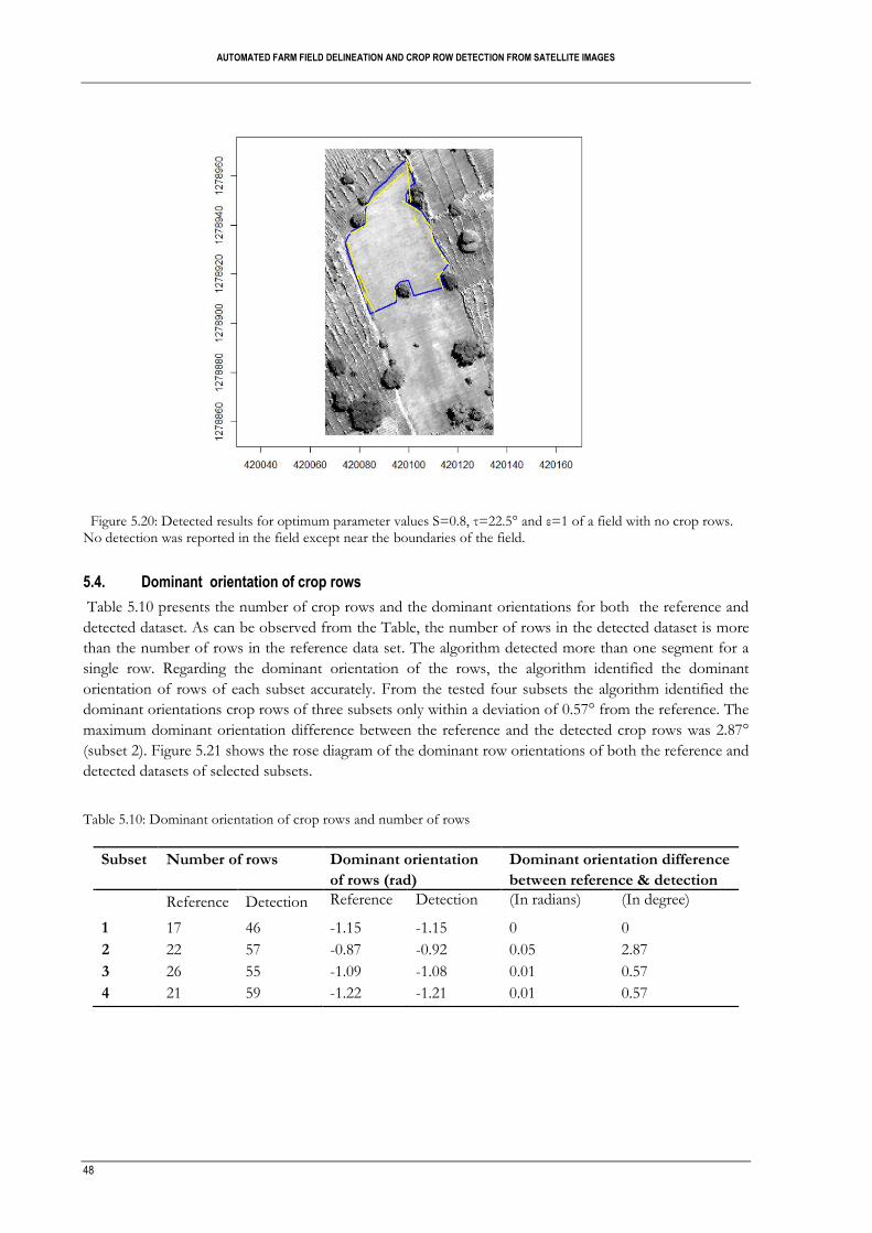
AUTOMATED FARM FIELD DELINEATION AND CROP ROW DETECTION FROM SATELLITE IMAGES
48
Figure 5.20: Detected results for optimum parameter values S=0.8, τ=22.5° and ε=1 of a field with no crop rows. No detection was reported in the field except near the boundaries of the field.
5.4. Dominant orientation of crop rows
Table 5.10 presents the number of crop rows and the dominant orientations for both the reference and
detected dataset. As can be observed from the Table, the number of rows in the detected dataset is more
than the number of rows in the reference data set. The algorithm detected more than one segment for a
single row. Regarding the dominant orientation of the rows, the algorithm identified the dominant
orientation of rows of each subset accurately. From the tested four subsets the algorithm identified the
dominant orientations crop rows of three subsets only within a deviation of 0.57° from the reference. The
maximum dominant orientation difference between the reference and the detected crop rows was 2.87°
(subset 2). Figure 5.21 shows the rose diagram of the dominant row orientations of both the reference and
detected datasets of selected subsets.
Table 5.10: Dominant orientation of crop rows and number of rows
Subset Number of rows Dominant orientation
of rows (rad)
Dominant orientation difference
between reference & detection
Reference Detection Reference Detection (In radians) (In degree)
1 17 46 -1.15 -1.15 0 0
2 22 57 -0.87 -0.92 0.05 2.87
3 26 55 -1.09 -1.08 0.01 0.57
4 21 59 -1.22 -1.21 0.01 0.57

AUTOMATED FARM FIELD DELINEATION AND CROP ROW DETECTION FROM SATELLITE IMAGES
49
(a) ( e)
(b) (f)
(c) (g)
(d) (h) Figure 5.21: Rose diagram of dominant orientation of crop rows of both reference and detection for four validation subsets. (a-d) are the orientations of reference rows and (e-h) are the orientations of their corresponding detected rows of subsets 1-4 respectively.

AUTOMATED FARM FIELD DELINEATION AND CROP ROW DETECTION FROM SATELLITE IMAGES
50
5.5. Spacing of Crop rows
Table 5.11 presents the average spacing of crop rows for both reference and automatically detected
datasets of four subsets. From the Table it is observed that the spacing between crop rows obtained by the
proposed method for all subsets are higher than the reference datasets. The maximum crop row spacing
difference between the reference dataset and the automatically detected dataset was 0.93 m (Subset 3) and
the minimum was 0.03 m (subset 1). Figure 5.22 shows the spacing of crop rows obtained by applying the
proposed procedure.
Table 5.11: Spacing of crop rows for four subsets.
(a) (b)
(c) (d)
Figure 5.22: Row spacing of four subsets. (a) Subset 1, (b) tuning subset, (c) subset 3, (d) subset 4. The vertical lines indicate the lags at which dominant frequencies are found.
Subset Average Crop rows spacing
(m)
Row spacing difference between
reference and detected (m)
Reference Detected
1 2.68 2.71 0.03
Tuning 2.94 3.61 0.67
3 4.48 5.41 0.93
4 5.3 5.41 0.11

AUTOMATED FARM FIELD DELINEATION AND CROP ROW DETECTION FROM SATELLITE IMAGES
51
6. DISCUSSION
This thesis explored two real applications of LSD algorithm on agricultural sector: field boundary
delineation and crop rows detection from satellite images. The results on field boundary delineation and
crop rows detection are discussed in section 6.1 and section 6.2 respectively.
Linear features are extracted from remote sensing imagery using the LSD algorithm taking into account
intensity differences between neighboring pixels. One of the most prominent advantages of remote
sensing is the multispectral nature of the observations. However, the LSD algorithm takes only a single
band as an input to detect linear segments. To make use of the advantage of the multispectral nature of
the observations, the research proposes to combine all available information present in different bands as
a single band before applying LSD algorithm. The LSD algorithm starts by calculating level-line angle for
each pixel based on pixel gradient. Level-line angles are used to form line-support regions. Each line-
support region is a potential candidate for a segment and is validated based on the calculation of a
Number of False Alarms (NFA) of the corresponding geometrical event (rectangle) associated with it. In
this research, all the eight bands of WorldView-2 image were used for field boundary delineation.
Multispectral information was explored by taking the vector sum of gradients of all eight bands. For crop
row detection panchromatic image band was used.
The automatically extracted line segments needed to be compared with the line segments in the reference
dataset to check the performance of the algorithm. The validation method presented in this research is
based on the method developed by Sidiropoulou Velidou et al. (2015), which uses the distance and
orientation difference between the reference dataset and automatically extracted dataset. To assess the
level of correspondence (correctness, completeness and positional accuracy) between the automatically
detected line segments with the reference dataset and to estimate optimal values of the internal parameters
of the LSD algorithm in the process of parameter tuning, two error ratios: ratio of missing detection (RM)
and ratio of false detection (RF) were defined.
6.1. Field boundary delineation
The parameters tuned were scale S, gradient threshold , angle tolerance and detection threshold The
optimal values of the three internal parameters obtained for this application were S = 1.0, and
The values of the two parameters and agreed with the ones proposed by Grompone von Gioi
et al. (2012). Some difference was observed on the scale parameter. For this application, the value of S that
minimized the sum errors RM+RF with lower standard deviation is S = 1.0, whereas the one proposed by
Grompone von Gioi et al. (2012) is S = 0.8.
The ratio of missing detection (RM) and the ratio of false detection (RF), defined in this validation
method, have shown the general pattern of the results for different parameter values by providing
quantitative measures and have been used for optimum parameter value selection. However, sometimes
these measures were misleading, especially for extreme values of parameters. Visual inspection of results
was necessary to ascertain whether these measures indeed reflect the optimum values or not.
The developed method is intended to detect all edges in an image by considering image intensity
differences. To this end, even edges that do not represent field boundaries can be detected and give false
detection for the purpose of this application. In the study area Mali, identifying edges that represent only

AUTOMATED FARM FIELD DELINEATION AND CROP ROW DETECTION FROM SATELLITE IMAGES
52
field boundaries from other features was a major problem. For example, the algorithm didn‟t make a
distinction between edges that correspond to field boundaries and other edges formed due to the shadow
of trees. Many line segments were extracted near trees in the field, which were actually not field
boundaries. This led to an over detection of segments and in turn increased the number of false
detections. Extracting trees from the image before detection could improve the detection results. On the
other hand, the algorithm missed many edges. One possible cause for missing detection could be a weak
contrast between neighboring fields.
In this research, an edge strength criterion was proposed to rank edges according to their strength. Two
basic attributes of line segments: contrast and steepness were calculated for this purpose. For the
automatically detected segments, edge strength analysis was performed using the developed criterion for
both successful and false detections. It was observed that both average contrast and steepness of
successful detections are higher than the corresponding values of false detections.
In this research, for the purpose of farm field boundary delineation, the LSD algorithm was tried on
texture bands. Different second order GLCM texture measures were explored and results were analyzed.
Studies have shown that incorporating texture measures could enhance the discrimination between
spectrally similar classes (Blaschke, 2010). When land covers exhibit similar spectral characteristics and
make classification difficult, the use of texture information is suggested as a potential solution (Lloyd et al.,
2004). In this study, however, the use of GLCM texture measures could not improve the results.
6.2. Crop rows detection
After the tuning process, the optimum values of the internal parameters obtained for this application
were S = 0.8, and . These optimum parameter values agree with the ones proposed by
Grompone von Gioi et al. (2012). For these selected parameter values, the ratio of missing and the ratio of
false detections are RM = 0.17 and RF = 0.48 respectively.
In this research, dominant orientation of crop rows was derived from the orientation of the automatically
detected lines (or specifically from the gradient orientation of pixels) and comparison was made with the
dominant orientations of reference dataset. The dominant orientations of crop rows of most of the
subsets were identified correctly by the proposed method. The capability of the algorithm in detecting the
spacing between the crop rows was also tested on four subsets of the image. The difference in row
spacing between the reference and the automatically detected datasets ranged from 0.03 m to 0.93 m. One
possible cause for this wide range could be the distribution of rows. Though most crop rows in a subset
followed similar patterns and assumed to have the same spacing, there were some irregularities on the row
spacing. This could have an effect on the automatically detected period (lag).
Accuracy assessment was conducted using the developed methodology to four subsets of the image. The
results showed the occurrence of both false and missing detections. The results also revealed that RF is
relatively higher than RM. One main cause for the occurrence of missing detection was the presence of
trees in the field. Visual observation of the results has shown that most missing detections were observed
for crop rows near trees. There were also changes in orientation of detected line segments for crop rows
that were occluded by trees. The cause for high RF was related to the width of crop rows. Each crop row
was represented by a single center line in the reference dataset. However, in most cases, the algorithm
extracted more than one segment for wider crop rows. This led an increase in the number of detected
crop rows (false detections). This problem could be minimized by adjusting the scale parameter, but could
not be totally avoided.

AUTOMATED FARM FIELD DELINEATION AND CROP ROW DETECTION FROM SATELLITE IMAGES
53
7. CONCLUSIONS AND RECOMMENDATIONS
7.1. Optimal parameter setting
Parameter setting of the algorithm has great effect on the quality of the results produced. That is proper
choice of parameter combination can lead to successful results. On the contrary, poor parameter setting
may lead to unsatisfactory results. Therefore, finding the optimum values of parameters of the LSD
algorithm that lead to successful detection of segments was an essential component of this study. The
choice of the best set of parameter setting was performed using the developed methodology by
minimizing the sum of errors of false and missing detections. In addition, visual inspection was performed
to ascertain whether these measures indeed reflect the optimum values or not.
The three internal parameters of the algorithm involved in the tuning process were scale S, angle tolerance
, and detection threshold . The scale parameter S involved in the algorithm helps to get a better representation of structure of certain features by controlling the spatial resolution of the image. The effect of the scale parameter on the detection results was very strong. Moreover, it controls the number of detected line segments. The number of detected line segments at low values of S was lower than the number at higher values of S for fixed values of other parameters. The second parameter tuned was angle
tolerance . This parameter was related to region growing. Low values are more restrictive for region growing, which does not allow pixels with large differences in gradient orientation to be included in the same line-support region. The third parameter tuned was detection threshold. This parameter was
responsible to distinguish -meaningful segments from all detected segments.
7.2. Assessment of the detection results
7.2.1. Field boundary delineation
The developed method for detecting field boundaries in areas with heterogeneous landscape was not as
successful as expected. The different approaches followed: extracting information from multiple bands,
using texture bands or image bands in detecting field boundaries do not give good results. Accuracy
assessment was performed following the proposed method by defining the two error ratios: the ratio of
missing detection and the ratio false detection. The results obtained for RM and RF were 0.78 and 0.73
respectively. The possible causes for these higher values of RM and RF were explored. The main cause for
the high ratio of false detection was the presence of trees in the field. Many line segments were detected
along the trees which didn‟t correspond to real field boundaries. One possible cause for missing detection
could be a weak contrast between neighboring fields. Extracting trees and other irrelevant linear features
like roads from the image before detection could improve the detection results. It is important to note that
the algorithm was tested on a single scene of the study area. It may give different (better) results for less
heterogeneous landscape.
7.2.2. Crop rows detection
Following the methodology for this application, the ratio of missing and the ratio of false detections on
the image subset for which the parameter tuning was performed are 0.17 and 0.48 respectively. The
capability of the algorithm in detecting the dominant orientation and the spacing between the crop rows
was tested on four different subsets of the image. The algorithm identified the dominant orientation of
crop rows correctly. From the tested four subsets, the maximum orientation difference between the
reference and the detected crop rows was 2.87° which was observed on a single subset. But for the other

AUTOMATED FARM FIELD DELINEATION AND CROP ROW DETECTION FROM SATELLITE IMAGES
54
three subsets the orientation differences between the two datasets were within 0.57°, which shows the
potential of the algorithm in detecting the dominant orientation of crop rows. The results of this research
show that the adopted methodology has a good potential in detecting crop rows automatically from
satellite images. However, it is important to note that the methodology was tested on different subsets of
the same image but not on a different image. Moreover, it is better to compare the results of this
algorithm to other standard methods that are used for automatic crop rows detection for detail analysis of
the results.
7.3. Recommendations
The quality of the reference dataset has great influence on the end results as well as on the conclusions
drawn from the results. The reference datasets in this research were digitized manually. Manual digitization
of field boundaries and crop rows is error prone. It could have its own influence on the results. Therefore,
whatever method applied, it is recommended to have accurate reference datasets. Moreover, knowledge of
the study area assists on the decisions to be made. In this research, parameter tuning was performed by
varying one parameter and keeping the others fixed. In future studies, it is recommended to develop a
procedure to find the optimum values of the parameters automatically. The procedures followed in
detecting the spacing between crop rows yielded reasonable results. These results could be improved by
combining the procedure with other techniques present in literature such as Fast Fourier Transform. The
region growing algorithm of the LSD is developed to detect straight linear features and rectangles are used
for validation. The algorithm can be modified and applied according to the required shape to be detected.

AUTOMATED FARM FIELD DELINEATION AND CROP ROW DETECTION FROM SATELLITE IMAGES
55
LIST OF REFERENCES
AGRA (2013). Africa Agriculture Status Reports. Retrieved August 24, 2015,
from http://agra-alliance.org/our-results/agra-status-reports/
Ali, Z. (2012). Assessing Usefulness of High-Resolution Satellite Imagery ( HRSI ) in GIS-based Cadastral
Land Information System. Journal of Settlements and Spatial Planning, 3, 4.
Ali, Z., Tuladhar, A., & Zevenbergen, J. (2012). An integrated approach for updating cadastral maps in
Pakistan using satellite remote sensing data. International Journal of Applied Earth Observation and
Geoinformation, 18, 386–398. http://doi.org/10.1016/j.jag.2012.03.008
Arivazhagan, S., & Ganesan, L. (2003). Texture segmentation using wavelet transform. Pattern Recognition
Letters, 24(16), 3197–3203. http://doi.org/10.1016/j.patrec.2003.08.005
Barry, P., & Coakley, R. (2013). Field accuracy test of RPAS photogrammetry. International Archives of the
Photogrammetry, Remote Sensing and Spatial Information Sciences - ISPRS Archives, 40(1W2), 27–31.
Retrieved from http://www.scopus.com/inward/record.url?eid=2-s2.0-
84924227025&partnerID=tZOtx3y1
Bhardwaj, S., & Mittal, A. (2012). A Survey on Various Edge Detector Techniques. Procedia Technology, 4,
220–226. http://doi.org/10.1016/j.protcy.2012.05.033
Blaschke, T. (2010). Object based image analysis for remote sensing. 5ISPRS6 Journal of Photogrammetry and
Remote Sensing, 65(1), 2–16. http://doi.org/10.1016/j.isprsjprs.2009.06.004
Bogaerts, T., & Zevenbergen, J. (2001). Cadastral systems - alternatives. Computers, Environment and Urban
Systems, 25, 325–337. http://doi.org/10.1016/S0198-9715(00)00051-X
Burns, J. B., Hanson, A. R., & Riseman, E. M. (1986). Extracting Straight Lines. IEEE Transactions on
Pattern Analysis and Machine Intelligence, PAMI-8(4), 425–455.
http://doi.org/10.1109/TPAMI.1986.4767808
Butenuth, M., Straub, M. B., & Heipke, C. (2004). Automatic extraction of field boundaries from aerial
imagery. KDNet Symposium on Knowledge-Based Services for the Public Sector, (pp. 3-4).
Chang, D., Nesbitt, K. V., & Wilkins, K. (2007). The gestalt principles of similarity and proximity apply to
both the haptic and visual grouping of elements. Conferences in Research and Practice in Information
Technology Series, 64(C), 79–86. http://doi.org/10.1109/WHC.2007.113
Da Costa, J. P., Michelet, F., Germain, C., Lavialle, O., & Grenier, G. (2007). Delineation of vine parcels
by segmentation of high resolution remote sensed images. Precision Agriculture, 8(1-2), 95–110.
http://doi.org/10.1007/s11119-007-9031-3
Dale, P. F., & McLaughlin, J. D. (1988). Land information management: an introduction with special reference to
cadastral problems in Third World countries . Clarendon Press. Retrieved from
http://books.google.com/books?id=MsDuAAAAMAAJ&pgis=1
Davis, L. S., Johns, S. A., & Aggarwal, J. K. (1979). Texture Analysis Using Generalized Cooccurrence
Matrices, (3).
Dekker, H. A. L. (2001). A new property regime in Kyrgyzstan; an investigation into the links between
land reform, food security, and economic development. Retrieved from
http://www.narcis.nl/publication/RecordID/oai%3Auva.nl%3A254573

AUTOMATED FARM FIELD DELINEATION AND CROP ROW DETECTION FROM SATELLITE IMAGES
56
Desolneux, A., Moisan, L., & Morel, J. M. (2003). Computational gestalts and perception thresholds.
Journal of Physiology Paris, 97(2-3), 311–324. http://doi.org/10.1016/j.jphysparis.2003.09.006
Desolneux, A., Moisan, L., Morel, J.-M., 2008 . From Gestalt Theory to Image analysis. Vol.34.
Springer New York.
Donnelly, G. J. (2012). Fundamentals of Land Ownership, Land Boundaries, and Surveying.
Intergovernmental Committee on Surveying and Mapping.Retrieved Retrieved November 24, 2015.Retrievd from
http://www.icsm.gov.au/index.html
Evans, C., Jones, R., Svalbe, I., & Berman, M. (2002). Segmenting multispectral landsat TM images into
field units. IEEE Transactions on Geoscience and Remote Sensing, 40(5), 1054–1064.
http://doi.org/10.1109/TGRS.2002.1010893
Faruquzzaman, a. B. M., Paiker, N. R., Arafat, J., Karim, Z., & Ali, M. A. (2008). Object segmentation
based on split and merge algorithm. IEEE Region 10 Annual International Conference,
Proceedings/TENCON, 2(2), 86–101. http://doi.org/10.1109/TENCON.2008.4766802
Epifanio, I., & Soille, P. (2007). Morphological texture features for unsupervised and supervised
segmentations of natural landscapes. IEEE Transactions on Geoscience and Remote Sensing, 45(4), 1074–
1083. http://doi.org/10.1109/TGRS.2006.890581
Ferencz, C., Bognár, P., Lichtenberger, J., Hamar, D., Tarcsai†, G., Timár, G., … Ferencz-Árkos, I.
(2004). Crop yield estimation by satellite remote sensing. International Journal of Remote Sensing, 25(20),
4113–4149. http://doi.org/10.1080/01431160410001698870
Franklin, S. E., Hall, R. J., Moskal, L. M., Maudie, A. J., & Lavigne, M. B. (2000). Incorporating texture
into classification of forest species composition from airborne multispectral images. International
Journal of Remote Sensing, 21(1), 61–79. http://doi.org/10.1080/014311600210993
Grompone von Gioi, R., Jakubowicz, J., Morel, J.-M., & Randall, G. (2008). On Straight Line Segment
Detection. Journal of Mathematical Imaging and Vision, 32(3), 313–347.
http://doi.org/10.1007/s10851-008-0102-5
Grompone von Gioi, R., Jakubowicz, J., Morel, J.-M., & Randall, G. (2012). LSD: a Line Segment
Detector. Image Processing On Line, 2, 35–55. http://doi.org/10.5201/ipol.2012.gjmr-lsd
Haralick, R. M., Shanmugam, K., & Dinstein, I. (1973). Textural Features for Image Classification. IEEE
Transactions on Systems, Man, and Cybernetics, 3(6). http://doi.org/10.1109/TSMC.1973.4309314
Harralick, R. M. (1979). Statistical and structural approach to texture. Proceeding of IEEE, 67(5), 786–804.
http://doi.org/10.1109/PROC.1979.11328
Harris, C., & Stephens, M. (1988). A Combined Corner and Edge Detector. Procedings of the Alvey Vision
Conference 1988, 147–151. http://doi.org/10.5244/C.2.23
Heipke, C., Mayer, H., & Wiedemann, C. Evaluation of automatic road extraction. IAPRS, “3D
Recontruction and Modeling of Topographic Objects.” Stuttgart, Vol. 32, September 17-19 1997
Ishida, T., Itagaki, S., Sasaki, Y., & Ando, H. (2004). Application of wavelet transform for extracting edges
of paddy fields from remotely sensed images. International Journal of Remote Sensing, 25(2), 347–
357. http://doi.org/10.1080/0143116031000115120
Jain, M., Mondal, P., DeFries, R. S., Small, C., & Galford, G. L. (2013). Mapping cropping intensity of
smallholder farms: A comparison of methods using multiple sensors. Remote Sensing of Environment,
AUTOMATED FARM FIELD DELINEATION AND CROP ROW DETECTION FROM SATELLITE IMAGES
57
134, 210–223. http://doi.org/10.1016/j.rse.2013.02.029
Janssen, L. L. F., & Molenaar, M. (1995). Terrain objects, their dynamics and their monitoring by the
integration of GIS and remote sensing. IEEE Transactions on Geoscience and Remote Sensing,
33(3), 749–758. http://doi.org/10.1109/36.387590
Ji, C. Y. (1996). Delineating agricultural field boundaries from TM imagery using dyadic wavelet
transforms. ISPRS Journal of Photogrammetry and Remote Sensing, 16(95), 268–283.
Jiang, H., Ngo, C., & Tan, H. (2006). Gestalt-based feature similarity measure in trademark database.
Pattern Recognition, 39(August 2005), 1–35. http://doi.org/10.1016/j.patcog.2005.08.012
Jing, Y, Zevenbergen, J& Ma, Z. (2011). Assessing Larsi-Integrated Participation Procedure for Urban
Adjudication in China, (May 18-22), 105. Retrieved from
http://www.itc.nl/library/papers_2011/msc/la/jing.pdf
Kurwakumire, E. (2014). Digital Cadastres Facilitating Land Information Management. South African
Journal of Geomatics, 3(1), 64–77.
Lengoiboni, M., van der Molen, P., & Bregt, A. K. (2011). Pastoralism within the cadastral system:
Seasonal interactions and access agreements between pastoralists and non-pastoralists in Northern
Kenya. Journal of Arid Environments, 75(5), 477–486. http://doi.org/10.1016/j.jaridenv.2010.12.011
Lloyd, C. D., Berberoglu, S., Curran, P. J., & Atkinson, P. M. (2004). A comparison of texture measures
for the per-field classification of Mediterranean land cover. International Journal of Remote Sensing,
25(19), 3943–3965. http://doi.org/10.1080/0143116042000192321
Lin, Y., Wang, C., Cheng, J., Chen, B., Jia, F., Chen, Z., & Li, J. (2015). Line segment extraction for large
scale unorganized point clouds. ISPRS Journal of Photogrammetry and Remote Sensing, 102, 172–183.
http://doi.org/10.1016/j.isprsjprs.2014.12.027
Meer, P., & Georgescu, B. (2001). Edge detection with embedded confidence. IEEE Transactions on Pattern
Analysis and Machine Intelligence, 23(12), 1351–1365. http://doi.org/10.1109/34.977560
Min, H. (2015). A Novel Level Set Model Based on Multi-scale Local Structure Operation for Texture
Image Segmentation. Journal of Information and Computational Science, 12(1), 9–20.
http://doi.org/10.12733/jics20105180
Moisan, L., & Morel, J.-M. (2000). Meaningful Alignments Agnes Desolneux. International Journal of
Computer Vision, 40(1), 7–23. http://doi.org/10.1.1.28.885
Morel, J., Randall, G., & Gioi, R. G. Von. (2010). LSD : A Fast Line Segment Detector with a False
Detection Control, 32(4), 722–732.
Mueller, M., Segl, K., & Kaufmann, H. (2004). Edge- and region-based segmentation technique for the
extraction of large, man-made objects in high-resolution satellite imagery. Pattern Recognition, 37(8),
1619–1628. http://doi.org/10.1016/j.patcog.2004.03.001
Nixon, M., & Aguado, A. (2012). Feature Extraction & Image Processing for Computer Vision, Third
Edition. In Feature Extraction & Image Processing for Computer Vision, Second Edition.
http://doi.org/10.1016/B978-0-12-396549-3.00003-3
Officers, A. (2012). Standard on Digital Cadastral Maps and Parcel Identifiers, (January), 1–18.
Pearsall, J. (1998). The New Oxford Dictionary of English. Oxford: Oxford University Press.
Rutzinger, M., Rottensteiner, F., & Pfeifer, N. (2009). Extraction From Airborne Laser Scanning. Ieee

AUTOMATED FARM FIELD DELINEATION AND CROP ROW DETECTION FROM SATELLITE IMAGES
58
Journal of Selected Topics in Applied Earth Observations and Remote Sensing, 2(1), 11–20.
Rydberg, A., Borgefors, G., & Member, S. (2001). Integrated Method for Boundary Delineation of
Agricultural Fields in Multispectral Satellite Images. IEEE Transactions on Geoscience and Remote Sensing,
39(11), 2514–2520.
Ryherd, S., & Woodcock, C. (1996). Combining Spectral and Texture Data in the Segmentation of
Remotely Sensed Images. Photogrammetric Engineering Remote Sensing, 62(2), 181–194. Retrieved from
http://www.asprs.org/publications/pers/96journal/february/1996_feb_181-194.pdf
Sainz-Costa, N., Ribeiro, A., Burgos-Artizzu, X. P., Guijarro, M., & Pajares, G. (2011). Mapping wide row
crops with video sequences acquired from a tractor moving at treatment speed. Sensors, 11(7),
7095–7109. http://doi.org/10.3390/s110707095
Sarkar, S., & Boyer, K. L. (1993). Perceptual organization in computer vision: a review and a proposal for
classificator extractor. IEEE Transactions on Systems, Man, and Cybernetics., 23(2), 382–399.
Sidiropoulou Velidou, D., Tolpekin, V. A., Stein, A., & Woldai, T. (2015). Use of Gestalt Theory and
Random Sets for Automatic Detection of Linear Geological Features. Mathematical Geosciences, 47(3),
249–276. http://doi.org/10.1007/s11004-015-9584-z
STARS Project, June 24-26, 2015, STARS general meeting, ITC, Enschede. Personal communication.
Tepper, M., Musé, P., Almansa, A., & Mejail, M. (2014). Finding contrasted and regular edges by a
contrario detection of periodic subsequences. Pattern Recognition, 47(1), 72–79.
http://doi.org/10.1016/j.patcog.2013.06.025
Tiwari, P. S., Pande, H., Kumar, M., & Dadhwal, V. K. (2009). Potential of IRS P-6 LISS IV for
agriculture field boundary delineation. Journal of Applied Remote Sensing, 3(1), 033528.
http://doi.org/10.1117/1.3133306
Torre, M., & Radeva, P. (2000). Agricultural-field extraction on aerial images by regioncompetition
algorithm. Proceedings 15th International Conference on Pattern Recognition. ICPR-2000, 1.
http://doi.org/10.1109/ICPR.2000.905337
Turker, M., & Kok, E. H. (2013). Field-based sub-boundary extraction from remote sensing imagery using
perceptual grouping. ISPRS Journal of Photogrammetry and Remote Sensing, 79, 106–121.
http://doi.org/10.1016/j.isprsjprs.2013.02.009
Ursani, A. A., Kpalma, K., Lelong, C. C. D., & Ronsin, J. (2012). Fusion of textural and spectral
information for tree crop and other agricultural cover mapping with very-high resolution satellite
images. IEEE Journal of Selected Topics in Applied Earth Observations and Remote Sensing, 5(1), 225–235.
http://doi.org/10.1109/JSTARS.2011.2170289
Williamson, I., & Ting, L. (2001). Land administration and cadastral trends - A framework for re-
engineering. Computers, Environment and Urban Systems, 25(4-5), 339–366.
http://doi.org/10.1016/S0198-9715(00)00053-3
Yan, L., & Roy, D. P. (2014). Automated crop field extraction from multi-temporal Web Enabled Landsat
Data. Remote Sensing of Environment, 144, 42–64. http://doi.org/10.1016/j.rse.2014.01.006
Yuan, J., & Cheriyadat, A. M. (2014, November). Learning to count buildings in diverse aerial scenes. In
Proceedings of the 22nd ACM SIGSPATIAL International Conference on Advances in Geographic Information
Systems (pp. 271-280). ACM.

AUTOMATED FARM FIELD DELINEATION AND CROP ROW DETECTION FROM SATELLITE IMAGES
59
Ziou, D., & Tabbone, S. (1998). Edge detection techniques - An overview. International Journal of Pattern
Recognition and Image Analysis, 8(4), 1–41.

AUTOMATED FARM FIELD DELINEATION AND CROP ROW DETECTION FROM SATELLITE IMAGES
60
APPENDIX
A. LSD results
Snapshot of LSD results showing different attributes: length, width, angle, NFA, end points of lines,
contrast and steepness.
B. LSD results on texture bands
(a) GLCM contrast for d=3 (b) GLCM mean for d = 3. Only a few segments were
detected.

AUTOMATED FARM FIELD DELINEATION AND CROP ROW DETECTION FROM SATELLITE IMAGES
61
C. Reference dataset for crop rows of different subsets.
(a) Subset1 (b) subset 2
(c) Subset 3 (d) Subset 4
(e) Tuning subset