AUTOMATED CAE PROCESS FOR THERMO …congress.cimne.com/iacm-eccomas2014/admin/files/filePaper/p2070.pdfThis is done here with Siemens Unigraphics NX 7.5 ... with lm cooling holes and

11th World Congress on Computational Mechanics (WCCM XI)5th European Conference on Computational Mechanics (ECCM V)

6th European Conference on Computational Fluid Dynamics (ECFD VI)E. Onate, J. Oliver and A. Huerta (Eds)

AUTOMATED CAE PROCESS FORTHERMO-MECHANICAL LIFING PREDICTION OF A

PARAMETERIZED TURBINE BLADE WITH INTERNALCOOLING

B.Nouri1 and A.Kuhhorn1

1 Chair of Structural Mechanics and Vehicle Vibrational Technology,Brandenburg University of Technology Cottbus,

Siemens-Halske-Ring 14, 03046 Cottbus Germany, [email protected]

Key words: CAE Process, Multiphysics Problems, Turbine, Cooling, Finite Element,Finite Volume, Coupled 1D and 3D CFD solver.

Abstract. For the benefit of higher overall thermodynamic efficiency in gas turbineengines, turbine blades are exposed to an increasingly high heat load, which exceeds themelting temperature of the metal airfoil. A system of internal cooling channels is requiredto provide sufficient cooling performance. However, the rising commercial pressure onengine manufacturers forces them to develop and produce engines with improved perfor-mance and reliability at lower cost in shorter periods than in the past. The turbine bladedesign techniques nowadays still carried out by optimizations based on steady state simula-tions. Nevertheless, a complete chain of processes beginning with the geometry and endingwith the lifing estimation is difficult, because of the very complex internal cooling channelgeometry, the lifing methods of single crystal alloys and the high operating temperature.Local flow phenomena and their associated impact on heat transfer may have significantimpact on turbine blade life. In this work, a CAE process is developed which combines thegeometry creation and the fluid-thermo-mechanical simulation of a high pressure turbineblade with a conventional cooling system. The sensibility of the S-N lifing curves has putincreased importance on the combining of the more accurate 3D CFD and fast 1D CFD.

1

B.Nouri and A.Kuhhorn

1 INTRODUCTION

In the drive for higher cycle efficiencies in gas turbine engines, turbine blades are ex-posed to an increasingly high heat load. The highly demanding requirements to endurethermal and structural loads, while aiming for high overall efficiency, lead to the designof a system with complex cooling channels. This in turn demands improvements of theinternal cooling system and a better understanding of the multidisciplinary prediction offluid solid interaction. A typical approach to enhance the internal cooling of the turbineblade is by casting angled low blockage ribs on the walls of the cooling channels. In orderto be able to simulate different settings of internal cooling channel, it is necessary to builda parametric CAD model of the sophisticated cooling blade, which must be capable ofreshaping the internal cooling system with all ribs and film cooling tubes.

The lifing analysis of the turbine airfoil requires a very accurate prediction of the in-ternal metal temperature. One of many lifing criteria of a turbine blade is the Low CycleFatigue (LCF) lifing where one cycle is defined by the maximum take-off flight condition.A critical section plane needs to be located with an automated routine, which recognizesin the spherical coordinate system the maximum principal stress gradient with the steep-est slope. The gradient will be compared with experimental data similar to the data ofNickel superalloys by Fleury & Ha 2001 [1]. This multiaxial fatigue analysis method isaccurate for the prediction of low cycle fatigue, but it requires a high density FEM mesh[1]. The simplified fatique analysis relationship calibrated by cyclic tests and the stressto number of life cycle curves are well described by Wu 2009 [2].

On the one hand such a demand of accurate temperature prediction can only be ful-filled with a complex 3D-CFD simulation of the whole internal cooling system. On theother hand a 1D-CFD model predicts the internal temperature within seconds. Nonethe-less, the 1D-CFD model has to be able to predict local heat transfer effects which areinduced by cooling features like ribs or rotational effects. Throughout in this investiga-tion, an approach is presented where 3D-CFD results are used to improve the 1D-CFDpredictions [3].

In this paper, the design and development of the CAE process is presented, along withthe current status. The paper begin with details on the parametrized CAD model of thehigh pressure turbine blade Smartblade and its advantages as complete expression basedmodel of a turbine blade with internal cooling. The identification of the 1D CFD flownetwork is expressed in the next section. The thermal simulation and the coupling to 3DCFD is shown in section 4. Finally it will be shown how the lifing is estimated with thestructural simulation. This investigation describes the building of a proccess chain whichwill end with an intelligent digital prototype (idq). As stated by [4] ”an idq can help toensure the required quality standard and it saves testing and simulation time”. Finally, aDesign of Experiment (DOE) example will be shown, where 10 different variations of theblade internal cooling system are assessed with the presented multi-disciplinary process.The design space evaluated turns out to have a range of life expectation from 1060 toapprox. 38000 cycles.

2


CAD •Generate 3D Geometry (turbine blade and internal cooling channels) •Identify 1D flow network for 1D CFD and 3D CFD-post

FVM •Automated meshing and calculation of the 3D CFD geometry •Automated post-processing with use of the 1D CFD parameter

FEM •Thermal simulation with coupled 1D-CFD (improved with 3D CFD investigations) •Structural simulation with automated lifing estimation

Figure 1: Complete CAE process

2 CAE process

The CAE process chain contains several different aspects of computer aided help forthe engineer (figure 1). First a CAD geometry model of the high pressure turbine bladewith internal cooling must be built. This is done here with Siemens Unigraphics NX 7.5and the interface NXOPEN. With this interface it is possible to create a turbine bladewith the external aerodynamic boundaries. This model contains complex internal coolingsystem with five cooling channels and two U-bends. However, information about the pathof the internal cooling system is missing. Therefore a tool has been developed which canidentify the internal 3D Path.

The goal of this CAE process is a lifing prediction, for which it is essential to predictthe local temperature with high accuracy. A possible but costly approach is to simulateexternal and internal cooling flow with 3D CFD. Nowadays as stated in [8], ”3D CFD isused with some confidence in industry and is considered essential as research tool”. Butthe complex geometry with film cooling holes and ribs will force the engineer to meshthe geometry with a high density discretization. Therefore a 1D CFD surrogate modelis used, that can take the information of 3D CFD and map an accurate heat transferprediction on the internal cooling channels.

3 SMARTBLADE AND SMARTCORE

For the purpose to be able to simulate different types of turbine blade geometries anexpression based model of the turbine blade with internal cooling system is required.These models are academic versions of a turbine blade with five cooling channels. Theexternal aerodynamic geometry is straight and not optimal, since outer aerodynamicshape is outside the scope of this work.

3.1 Smartblade

The smartblade is an expression driven process which includes CAD scripting in NXwith NXOpen. The inputs for this model are the firtree type, the tip type and the externalaerodynamic surfaces (pressure side and suction side). It enables to choose between severaltypes of tip and feet shapes which fit with the size of the airfoil.

3


Input external aerodynamic shape

and build skeleton line Internal

core

Cooling channel design

3D CFD featured internal

core

Defeatured metal blade

Figure 2: Smartblade + Smartcore: A parametrized scripted UG method to generate a featured CFDgeometry (top right air volume is solid) and a defeatured metal blade model (buttom right no coolingfeatures)

3.2 Smartcore

This tool is able to generate a complete cooling system with a variable number ofinternal cooling channels and bends. It also can generate cooling enhancement features,such as ribs and film cooling holes. It delivers a fully blade model defined by expressionswith a high flexible (more than 1010 possible set of expressions) set of variation. For thehere presented numerical investigation, a cooling geometry with five cooling channels iscreated with low blockage 45 ribs.

4 THERMAL SIMULATION WITH 3D AND 1D CFD

4.1 1D CFD Flow

A surrogate model of the complex internal 3D flow structure is developed. This 1D CFDsurrogate model is about 10000 times faster than full 3D CFD but it requires accurateinformation about the distribution of the internal heat transfer coefficient (figure 3).However it also requires the basic geometric information of the internal system which willvary with every variation of the Smartcore. To obtain this information automatically, atool in UG NX 7.5 with NXOpen was developed which can identify the internal coolinggeometry. It extracts directly from the CAD model the XYZ Data of the middle points(every channel will be analyzed on 30 positions) and the relevant fluid data. For theinternal cooling system with low blockage ribs the following parameters are relevant:

• hydraulic diameter Dh

• area A

• perimeter P

• aspect ratio AR (width to height relationship in the internal cooling channel)

• all attached cooling features (ribs or films)

4


Surrogate model of the complex 3D internal cooling

system with a 1D CFD Network

geometry

Thermal FE Simulation with internal 1D CFD

Code

Figure 3: Structural high density mesh

4.2 3D CFD Flow

The pressure based solver used for the analysis is Fluent 14.0. The velocity pressurecoupling method used was the coupled method. The material model of air is an ideal gasfor density with Sutherland 3 coefficient method for the viscosity. The K-Omega withSST turbulence model was chosen for a compromise of good results and good convergencebehaviour. The convergence criteria are constant low residuals (less than 1e-4) and amaximum difference of 0.01% of the total surface heat flux integral of a section of 5 ribsover 100 iterations.

Table 1: Settings for 3D CFD

CFD Setting-FLUENT 14.0

cell zone inlet Mass flow inlet normal to boundary

cell zone outlet Pressure outlet

solid walls Wall temperature

solver Pressure based, implicit 2nd order discretization

turbulence K-omega SST

The mesh is a combination of tetrahedral and prismatic elements. The meshing toolwhich has been used is ICEM from ANSYS. It was created with 16 prismatic layers onall walls. The aim was a non-dimensional wall distance yplus of 0.3 for ribbed and thesmooth surfaces. Each rib is discretized with more than 6 elements in flow direction.The pressure and suctions side are in general much finer meshed than the plenum or thesurfaces without ribs.For the post processing a method was developed which can use the 1D CFD parameter

5


for the 3D CFD heat transfer distribution (figure 4). To acquire the Nusselt number ratioNu/Nu0, several parameters must be extracted as mass flow averaged surface integral inthe post processor. The hydraulic diameter is calculated according to:

Dh = 4(Area/Perimeter) (1)

Several sections on different positions S (channel position from cooling channel beginningto tip) have been made to get the mass averaged local total bulk temperature and thelocal mean velocity. The Reynolds number for channels is defined by:

Re =ρUb(S)Dh

µ(2)

where ρ is the local density and Ub is the mean velocity. Polynomial functions are used toapproximate the local bulk flow temperature TB along the S coordinate in the channel.With the local bulk temperature the heat transfer coefficient h is calculated:

h = q/(Tw − Tb(S)) (3)

The local Nusselt number is calculated with the local heat transfer coefficient h and thelocal thermal conductivity:

Nu = hDh/(k) (4)

The fully developed Nusselt number for a turbulent stationary smooth pipe is given by:

Nu0 = 0.023Re(S)0.8Pr0.4 (5)

This is the equation from Dittus Boelter/McAdams [1] for smooth pipe where Pr isthe local molecular Prandtl number.

Build with 1D CFD Data a

Nusselt number distribution for

the whole internal system

Surface perpendicular to

the flow direction on position S

𝐴(𝑆),𝑃(𝑆),𝐷ℎ(𝑆),𝑈𝑏 𝑆 ,𝑇𝑏 𝑆 ,𝑅𝑅 𝑆 …

Figure 4: Automated CFD Post processing with use of 1D CFD parameter

6


4.3 1D and 3D CFD combination

There are three important local Nusselt number surface effects which need to be takeninto account for the different cooling flow channels:

• The local enhancement due to the asymmetric geometry of the 45 rib

• The rotational effect

• Impingement at inlet of the film cooling holes

All effects cause high local enhancement of the Nusselt number ratio and therefore shouldbe applied as boundary condition to the thermal simulation of defeatured geometries forlifing simulations and for an accurate temperature prediction. However, since the 1DCFD code in the beginning of this investigation was not able to map local heat transfersolutions a coupled solver has been written, in which the 1D central flow is normalized bythe local effects which are mapped to this 1D CFD channel. The cooling channel wallsare divided into four different sides and are named according to the position in a turbineblade.

• PS- is the pressure side (Coriolis force in outwards directed rotating cooling channelis directed towards PS)

• SS- is the suction side of the cooling channel

• LE- is the side nearest to the blade leading edge

• TE- is the side nearest to the blade trailing edge

In figure 5 the mapping method is shown for 2 different cooling channels with differentheight to width ratio (aspect ratio AR), the effect of rotation is a result of the shape ofthe cooling channel.The function of the Nusselt number ratio distribution is plotted as afunction of X. Where X is a normalized distance parameter starting in the corner PS LEand is extending anti clockwise around the cooling channel (figure 5). The maximum ofX is 4, each side is 1 long for AR=1. For AR=0.5 the maximum length of X is 3 becausetwo sides are shorter.

The distribution of the Nusselt number ratio disparities between the rotational frameand the stationary frame is significant for small AR. For AR=1 there is a significantdifference of the shape of the distribution on the LE and TE side.

7


AR=0.5

1D CFD point inside the blade

Distribution around the 1D

CFD point

1D CFD flow path

Figure 5: Nusselt number ratio distribution for a 4 wall geometrie with differen aspect ratios and rotationnumbers

5 MECHANICAL FE SIMULATION AND LIFING

5.1 FE mechanical

The mesh discretization for the finite element method of the turbine blade is shown infigure 6. This defeatured blade is represented by a solid airfoil attached to a 6% sectionof the disc platform. Since this investigation is focused on the airfoil section, the platformonly serves as the elastic boundary condition. The external temperature and pressuredistributions are obtained from a 3D fluid simulation combined with a 2D film coolingefficiency calculation for the hot external surface. The external geometry and boundarycondition is set constant for all obtained DOE results. The turbine rotates at 12000 rpm.

8


High density discretized turbine blade for thermal and

structural FE simulation ~1 million elements

Defeatured model no film cooling holes or ribs are

included

Figure 6: Structural high density mesh

The results of the structural simulation showed a high peak of the maximum principalsurface stress at the first U-bend where the flow is redirected from cooling channel 2 tocooling channel 3 (figure 7). Although this is not the only region with a significant highlocal surface stress the following lifing DOE in this paper will focus on this region.

Static mechanical analysis on the defeatured geometry normalized max principal

stress 1 0

Cooling channel 2

First U-bend

Figure 7: Maximum principal stress at intenal surface first U-bend

5.2 Lifing Assesssment

A lifing model generally calculates the number of cycles to failure for a certain compo-nent to a specific load sequence. The component in this investigation is the turbine bladewith internal cooling channel and the load sequence is the maximum take off condition.The basis of this method was the estimation of component life through the constructionand use of empirical stress-life (S-N) curves, for the relevant materials. There is highconfidence on this method, as stated by [10]: ”The methodology has been extensivelyvalidated against a database of fatigue results for a typical engine alloy, and has beendemonstrated to provide accurate estimates of specimen and component life under ex-treme combinations of both stress and volume”. The LCF data from laboratory test areused to estimate the life of high pressure turbine components with stress concentrationfeatures such as connection channels or bends, since it is believed that with the con-straint of the surrounding elastic material, the local deformation behavior is leaning more

9


0

0.4

0.8

1.2

1.6

2

100 1000 10000 100000 1000000

Mea

n st

ress

nor

mal

ized

de

viat

ion

Expected minimum LCF life cycles

S-N curve single crystal alloy 850°C

Figure 8: Normalized experimental S-N curve of an nickel based single crystal alloy

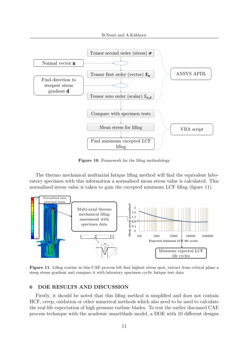
towards strain-controlled condition. A good description of the heated specimen and thederivation of the typical S-N curves are in [11]. In figure 8 a normalized mean stress graphof this tests is shown. The sensibility is enormous for a very low change of the mean stressvalue the lifing can increase or decrease by factor 10, especially around 10.000 to 100.000estimated minimum life cycles.

The stress tensor must be reduced twice to get the scalar value. Firstly, a critical planenormal to the spot is selected, within this plane a routine will check and compare all stressgradients and find a direction with the most critical internal stress distribution (figure9 and 10). This is a multiaxil LCF lifing methodology similar to the method describedby [5]. The combination of d and n describes a critical cutplane, it is exceptet that themaximum of the cyclic metal degradation is in the direction d.

Sn,d = d · Sn = d · (n · σ) (6)

Local region with highest surface stress

n d

𝜃 𝑙

Internal surface

Critical direction d Multiaxial thermo-mechanical lifing assessment

critical section

Figure 9: Sketch of critical cut plane and the finding of the steep stress gradient

10


Tensor second order (stress) 𝝈

Tensor first order (vector) 𝑺𝒏

Tensor zero order (scalar) 𝑆𝑛,𝑑

Normal vector n

Find direction to steepest stress

gradient d

Compare with specimen tests

Mean stress for lifing

ANSYS APDL

VBA script

Find minimum excepted LCF lifing

Figure 10: Framework for the lifing methodology

The thermo mechanical multiaxial fatique lifing method will find the equivalent labo-ratory specimen with this information a normalized mean stress value is calculated. Thisnormalized stress value is taken to gain the excepted minimum LCF lifing (figure 11).

00.40.81.21.6

2

100 1000 10000 100000 1000000Mea

n st

ress

nor

mal

ized

Expected minimum LCF life cycles

Multi-axial thermo mechanical lifing assessment with specimen data

Minimum expected LCF life cycles

1 0

Normalized max principal stress

Figure 11: Lifing routine in this CAE process left find highest stress spot, extract from critical plane asteep stress gradient and compare it with labratory specimen cyclic fatique test data

6 DOE RESULTS AND DISCUSSION

Firstly, it should be noted that this lifing method is simplified and does not containHCF, creep, oxidation or other numerical methods which also need to be used to calculatethe real life expectation of high pressure turbine blades. To test the earlier discussed CAEprocess technique with the academic smartblade model, a DOE with 10 different designs

11


Smartblade & Smartcore

2x featured internal

geometries

10 x defeatured blade geometries

3D CFD web wall angle=0°

5x 1D CFD & thermal FE AR(cooling channel 2)

=0.194-0.295

5X Structural FE with

automated lifing

3D CFD web wall angle=35°

5x 1D CFD & thermal FE AR(cooling channel 2)

=0.19-0.298

5X Structural FE with

automated lifing

Figure 12: Sketch of the DOE CAE process chain

0.150.170.190.210.230.250.270.290.31

100 1000 10000 100000

AR

coo

ling

chan

nel 2

Minimum LCF life in cycles at the first bend

Web wall angle=0°

Web wall angle=35°

Reference design

Best design

Dire

ctio

n of

ro

tatio

n Figure 13: Lifing results of the DOE and description of the web wall angle

was performed and is shown in figure 12. The external heat transfer boundary conditionand geometry are kept constant for all computations of the temperature and lifing.

The results of the lifing DOE put into manifest that with a skew ∆β of the web wallangle (the angle of the walls between the cooling channels) the lifing estimation can rise upto nearly 38.000 LCF cycles until the expected failure (figure 13). Figure 14 presents theinternal reference cooling geometry of the Smartcore model, together with the geometrythat achieves the best excepted lifing prediction.

6.1 Discussion

Table 2 brings some data explanation in order to understand the difference of nearly38.000 excepted minimum life cycles between the reference design and the best design,which have the same external boundary condition, the amount of coolant flow, and rotat-ing number.The heat transfer is in the best design significantly higher, therefore the temperature islower. Additionally, this lower temperature is combined with a lower maximum principalstress at the spot with the highest surface stress in the first bend. The sensibility of theS-N curve is responsible that a very small variation of the mean stress value can result ina massive variation of the minimum excepted LCF lifing (figure 8). As described by J.C.

12


Reference design AR<0.2 channel 2 web wall angle=0°

Best design in DOE AR>0.28 channel 2 web wall angle=35°

Cooling channel 2

Figure 14: Comparison internal cooling design Reference design left best DOE lifing result right. Viewfrom suction side

Han 2013 [7] ”It is widely accepted that the life of a turbine blade can be reduced by halfif the temperature prediction of the metal blade is off by only 30C.” It should be notedthat for this particular case not only the maximum temperature and surface peak stressdecreased, the parameter which influenced the lifing most is the internal rapid change ofthe stress in direction d caused by the wider channel 2 and the web wall angle change.

Table 2: Settings for 3D CFD

Data on the spot with highest local principal stress at the suction side of the first bend

Difference between the best (AR=0.29 and Δ𝛽 = 35°) and reference design (AR=0.192 and 𝛽 = 0°)

Temperature -25.54K

Internal heat transfer coefficient +20.7%[W/m²K]

Max principal stress -14,5%[Pa]

Minimum LCF lifing Factor 36,02

The higher heat transfer can be explained of the skewed web wall angle as shown in[3] a skew of the web wall angle by 35 does distribute the cooling flow more uniformbetween pressure and suction side of the cooling channel (figure 15). The correctionfactor for ribbed channels with different aspect ratio is in good comparison with theexperimental setup from Azad 2007 [6]. Without the influence of the internal metal stressdistribution, which is responsible for a significant lower value of mean stress, and onlywith consideration of temperature and stress decrease between reference and the bestdesign the lifing factor would only increase to 12 and not to 36.

13


11.051.1

1.151.2

1.251.3

1.351.4

1.45

0 0.1 0.2 0.3 0.4 0.5

AR=0.5, web wall angle=0°

AR=0.5, web wall angle=35°

𝑁𝑁

𝑁𝑁 0

(𝑃𝑃)

/𝑁𝑁

𝑁𝑁 0

(𝑃𝑃)

𝑅𝑅

Figure 15: Influence of the web wall angle and the distribution of coolant flow efficiency between pressureside and suction side of the internal cooling channel walls [3]

7 CONCLUSIONS

In order to generate and simulate an intelligent digital prototype of a high pressureturbine blade in an CAE environment it is important to use an innovative design approachand implement accurate physical correlations for a fast solver which than gives the userthe ability to optimize the design of a complex internal cooling flow geometry. Thecombination of 3D CFD and 1D CFD is used to reduce the simulation time by a factorof 10000, however the outcome is a very accurate 3D thermal field. The enhanced 1DCFD model is essential because the 3D Fluid forces have a small impact on surfacetemperature and heat transfer but a massiv influence on the lifing factor. The automatedlifing simulation with LCF can deliver a good start point for the real lifing simulationwith HCF lifing and TBC lifing estimation. Generally it can be said that this processcould be used with real shaped external blade geometries.

8 OUTLOOK

This CAE process chain does not include a tool for oxidation or HCF lifing. Additionalto the multiaxial LCF model, a multiaxial formulated creep model could be implemented,as shown by [9]. Moreover, it opened potential to automate investigations for newercooling approaches. Unregular V shaped ribs and grooves with a high TPF could beimplemented and it would bring the possibility for the first assessment of unconventionalcooling geometries like cyclone cooling channels.

9 ACKNOWLEDGMENTS

This work has been carried out in collaboration with Rolls-Royce Deutschland as partof the research project VIT 3 (Virtual Turbomachinery, contract no. 80142272) fundedby the State of Brandenburg and Rolls-Royce Deutschland. Rolls-Royce Deutschlandspermission to publish this work is greatly acknowledged. Special thanks also to RolandParchem from Rolls-Royce for his ideas and guidance.

14


REFERENCES

[1] Fleury, E. & Ha, J.S.:Thermomechanical fatigue behaviour of nickel base superalloyIN738LC: Part 2–Lifetime prediction., T17, pp. 1087-1092.

[2] Wu, X.J., Yandt, S. & Zhang, Z. (2009).:A Framework of Integrated Creep-FatigueModelling , Proceedings of the ASME Turbo Expo 2009, GT2009-59087, June 8-12,2009, Orlando, Florida, USA.

[3] Nouri, B., Lehmann, K., Kuhhorn, A. Investigations on nusselt number enhancementin ribbed rectangular turbine blade cooling channels of different aspect ratios androtation numbers Paper GT2013-94710 , Proceedings of ASME Turbo Expo 2013,June 3-7, San Antonio, Texas, USA

[4] F. Linares, Z. Zamperin, N. Gramegna, L. Furlan: iDP approach to quality assess-ment and improvement of diecasting process , TCN-CAE 2003, International confer-ence on Cae and Computational Technologies for industry.

[5] Gaier C., Hofwimmer K., H. Dannbauer H.Genaue und effiziente Methode zur mul-tiaxialen Betriebsfestigkeitsanalyse Nafems online magazin , Nr. 4, p.79-89, 2013.

[6] Azad, G. S., Uddin, M. J., Han, J. C., Moon, H. K., and Glezer, B., 2002, HeatTransfer in a Two-Pass Rectangular Rotating Channel with 45-Deg Angled Rib Tur-bulators , ASME J. Turbomachinery, Vol. 124, pp. 251-259.

[7] Han, J.C. ; Dutta, S. ; Ekkad, S.: Gas turbine heat transfer and cooling technology .2nd ed. Boca Raton and Fla : CRC Press, 2013. ISBN 9781439855683

[8] J. W. Chew and N. J. Hills, Computational fluid dynamics for turbomachinery in-ternal air systems , (eng),Philos Trans A Math Phys Eng Sci, vol. 365, no. 1859, pp.2587 2611, 2007.

[9] Rauer, G., Kuhhorn, A., Springmann, M. Residual Stress Simulation of an AeroEngine Disc during Heat Treatment Proceedings of the 6th European Congress onComputational Methods in Applied Sciences and Engineering (ECCOMAS 2012),September 10-14, 2012, Vienna, Austria, ISBN: 978-3-9502481-9-7

[10] Shepherd D.P., and Williams,S.J. New Lifing Methodology for Engine Fracture Crit-ical Parts Aging Mechanisms and Control. Symposium Part A - Developments inComputational Aero- and Hydro-Acoustics. Symposium Part B - Monitoring andManagement of Gas Turbine Fleets for Extended Life and Reduced Costs 2001

[11] Lindemann J., Roth-Fagaraseanu D. and Wagner H. Effect of Shot Peening on FatiguePerformance of Gamma Titanium Aluminides Conf Proc: ICSP-8 Sept. 16-20, 2002Garmisch-Partenkirchen, Germany

15


Table 3: Nomenclature and Abbreviation

PS Pressure side TE Trailing edge side SS Suction side LE Leading edge side AR Channel aspect ratio DH Channel hydraulic diameter 2WH/(W+H) d Direction to steepest gradient k Local thermal conductivity of air Pr Prandtl number Local surface heat flux

LCF HCF

Low cycle fatique High cycle fatique

Nu Nusselt Number Nu0 Nusselt number for fully developed turbulent flow in a

stationary smooth pipe Re Reynolds number Ro Rotation number: ΩDH /Ub S Distance from the inlet of the rectangular ribbed duct Tb Bulk mean temperature Tw Local wall temperature W Flow channel width AR Aspect ratio width to height W/H Ub Bulk flow velocity of the cooling air X Length variable on the cooled surface perpendicular to the Z-

axis 𝛽 Orientation angle from cooling channel to the rotation axis

Web wall angle 𝜌 Local air density 𝝈 Stress Tensor 𝜇 Local air viscosity

16

Documents

AUTOMATED CAE PROCESS FOR THERMO …congress.cimne.com/iacm-eccomas2014/admin/files/filePaper/p2070.pdfThis is done here with Siemens Unigraphics NX 7.5 ... with lm cooling holes and