1 Lenjani et al.

Automated Building Image Extraction from 360-degree Panoramas for Post-Disaster Evaluation

Automated Building Image Extraction from

360-degree Panoramas for Post-Disaster Evaluation

Ali Lenjani1, Chul Min Yeum2*, Shirley Dyke1,3 and Ilias Bilionis1

1School of Mechanical Engineering, Purdue University, West Lafayette, IN 47907, United States

2Department of Civil and Environmental Engineering, University of Waterloo, ON, N2L 3G1, Canada 3Lyles School of Civil Engineering, Purdue University, West Lafayette, IN 47907, United States

Abstract: After a disaster, teams of structural engineers

collect vast amounts of images from damaged buildings to

obtain new knowledge and extract lessons from the event.

However, in many cases, the images collected are captured

without sufficient spatial context. When damage is severe, it

may be quite difficult to even recognize the building. Accessing

images of the pre-disaster condition of those buildings is

required to accurately identify the cause of the failure or the

actual loss in the building. Here, to address this issue, we

develop a method to automatically extract pre-event building

images from 360o panorama images (panoramas). By providing

a geotagged image collected near the target building as the

input, panoramas close to the input image location are

automatically downloaded through street view services (e.g.,

Google or Bing in the United States). By computing the

geometric relationship between the panoramas and the target

building, the most suitable projection direction for each

panorama is identified to generate high-quality 2D images of

the building. Region-based convolutional neural networks are

exploited to recognize the building within those 2D images.

Several panoramas are used so that the detected building

images provide various viewpoints of the building. To

demonstrate the capability of the technique, we consider

residential buildings in Holiday Beach, Texas, United States

which experienced significant devastation in Hurricane Harvey

in 2017. Using geotagged images gathered during actual post

disaster building reconnaissance missions, we verify the method

by successfully extracting residential building images from

Google Street View images, which were captured before the

event.

1 INTRODUCTION

In the aftermath of the recent severe hurricanes across

Florida, the Gulf of Mexico and Puerto Rico, and the

devastating clusters of earthquakes in Mexico, significant

causalities and economic losses resulted from failures of the

built environment. Millions of residents were forced to rebuild

or repair their buildings (Smith, 2018). Understanding the

nature of the risk to our building inventory is essential for

making decisions that reduce risk, mitigate losses, and enhance

the ability of a community to recover after a disaster.

There is strong agreement in the engineering community that

engineers can and should learn much more from the

consequences of each disaster than we do today (Gutmann,

2011). As part of these procedures to enable the learning

process, post-event reconnaissance teams are dispatched after

disasters to investigate damaged buildings and to collect

perishable data (Sim et al., 2016; NCREE, 2016; Brando et al.,

2017; Kijewski-Correa et al., 2018a, 2018b; Roueche et al.,

2018). For instance, Fig. 1 shows samples of images collected

from actual post-hurricane reconnaissance missions (Katrina in

2 Lenjani et al.

2005 and Harvey in 2017). During a typical mission, images are

collected from many buildings, and these images are used to

document findings and observations in the field. Meaningful

scenes are captured from particular viewpoints to provide visual

evidence of damaged/undamaged buildings or their

components. Such data allow researchers to distil important

lessons that will improve the safety and reliability of our

buildings, as well as the resilience of our communities

(Jahanshahi et al., 2009; Gao and Mosalam, 2018; Cha et al.,

2017; Cha et al., 2018; Hoskere et al., 2018; Liang, 2018; Li et

al., 2018; Xue and Li, 2018; Yeum et al., 2018b; Xu et al.,

2019). In the United States, the National Science Foundation

recently funded a unique RAPID facility within the NHERI

(Natural Hazards Engineering Research Infrastructure) network

that is dedicated to supporting reconnaissance teams as they

collect such field data (NSF, 2014).

To understand the probable causes of damage, it is essential

to use the post-disaster images together with pre-disaster views

of the original condition of the structure. Suppose that the target

buildings are severely damaged, like those in Fig. 1. In this case,

pictures of remnants of building frames and associated debris

do not have significant value unless information regarding their

pre-event condition is also provided. Pre-disaster building

images contain abundant information regarding building-level

characteristics (e.g., number of floors, architecture/structural

style) and details about components (e.g., roof style, windows

opening, column locations). This information is critical for

understanding the root causes of damage during the event

(Suppasri et al., 2013).

Recent advances in sensors, sensing platforms, and data

storage enable automated solutions for structural engineering

problems (Rafiei and Adeli, 2017; Choi et al., 2018; Gao and

Mosalam, 2018; Hoskere et al., 2018; Yeum et al., 2015, 2018a,

2018c). One of the best resources available to observe buildings

in their pre-disaster condition is street view images (Anguelov

et al., 2010). Through such services, a sequence of 360-degree

panorama images (hereafter, panoramas) captured along nearby

streets enables all-around views at each location. Many internet-

based map service providers offer a street view service, such as

Google or Bing in the United States or Tencent in China, and

these service providers store a sufficiently broad temporal and

geographic range of panoramas. Using the GPS coordinates of

a particular building, several external views of that building can

be extracted. Thus, facilitating the realistic use of such data is

expected to yield much more granular information regarding the

pre-event state of the buildings in a region.

In this study, we develop an automated technique to detect

and extract curated pre-event building images from typical

street view panoramas. This technique is intended to support

research investigating the impact of disasters on a building

inventory. The extracted images capture the external

appearance of a building from several viewpoints. As a

preliminary step, a classifier is first trained to detect buildings

within images using a large ground-truth building image set.

The region-based convolutional neural network algorithm is

exploited to design a robust building classifier (Ren et al.,

2017). Ideally, in the real-world application of this technique, a

user can simply provide, as the input, a geotagged image (or

similarly, a GPS coordinate) recorded near the target building,

and the rest of the process is fully automated. The physical

location of the target building is estimated using the geometric

relationship between the panoramas and the building. Then, the

optimal projection plane for each of the panoramas is

determined to produce a high resolution, undistorted 2D

building image from the corresponding panoramas. The region

(position) of the building on each 2D image is determined using

the trained classifier, and an image of the building is extracted

from each 2D image. The output of the technique is a set of

several undistorted images of the building, taken from all

available viewpoints. Generating multiple image reduces the

possibility of an obstruction (e.g. trees, cars or fences) in a

particular viewpoint and, thus, enables robust visual

assessment. Also, by using this procedure with data from

multiple street view services, a user can collect street view

images obtained over many past years to observe the target

building over time. The performance of the technique

developed here is demonstrated and validated using residential

buildings affected by Hurricane Harvey (in 2017) in Holiday

Beach, TX. Real-world post-event reconnaissance images,

collected by engineers in the field, are used as the input for this

validation, and pre-disaster views of the buildings in those

reconnaissance images are automatically extracted from Google

Street View (Shet, 2014).

The major contribution of this study is to provide a practical

and feasible solution to a problem that is grounded in the needs

of engineers who seek to learn from disasters. With the

capability to analyze post-disaster building scenarios by readily

accessing pre-disaster images and post-disaster data, engineers

are equipped with the tools to rapidly develop a greater

understanding of the performance of our infrastructure. The

technique developed automatically provides high-resolution

undistorted multiple view pre-event images of each building.

The key technical contributions are in automatically removing

the inherent distortion of the 2D projection of panorama images

and in rapidly extracting a set of images of each post-disaster

(a) (b)

Figure 1. Sample images collected during post-event

building reconnaissance missions: (a) Hurricane Katrina in

2005, and (b) Hurricane Harvey in 2017 (Courtesy of

Timothy P. Marshall and Thomas P. Smith, respectively).

3

target building with multiple viewpoints. Additionally, a side

benefit of this technique is the ability to exploit the vast amounts

of legacy visual data that exist from past disasters. With such

visual databases being collected and established, and the cost of

image acquisition and data storage decreasing, this technique

offers just one example of how to automate the reuse of existing

data through the novel application of state-of-art computer

vision algorithms to solve real-world problems.

The paper is structured as follows. First, the challenges in

using street view images for our application are introduced in

Section 2. Section 3 provides a brief introduction of the

convolutional neural network-based object detection

methodology, called region-based convolutional neural network

(Ren et al., 2015). The technical details of the technique are

explained in Section 3, and in Section 4, it is demonstrated using

Google Street View images gathered from Holiday Beach in

Texas, United States, which was heavily affected by Hurricane

Harvey in 2017. The summary and conclusions of this study are

presented in Section 5.

2 Problem Statement

The 360-degree panorama image is an image that is able to

capture all around (spherical) scenes from a given location. The

merit of panoramas is that, after the data are collected, one may

quickly navigate to scenes of interest in any direction from the

given location. This advantage does not apply to 2D images.

With 2D images, the direction in which the data are being

collected must be determined at the data collection stage. Thus,

panoramas are quite useful when for reconnaissance because

when they are collected from multiple locations, several

different external views of a given building are automatically

recorded (e.g., front or sides). In the panorama viewers typically

implemented by street view service providers, 2D rectilinear

images are rendered from the panoramas in real-time based on

the selected viewing direction (represented by a pitch and yaw)

and zoom level (Google Developers, 2018a). When rendered in

this way, the rectilinear images are just the 2D images that would

typically be obtained with an ordinary (non-fisheye) camera.

These images represent scenes in the world as people actually

see and perceive them. For instance, a straight line in the 3D

world is represented as a straight line in the corresponding

rectilinear image (Kweon, 2010). Such viewers also frequently

overlay directional arrows to enable a user to move to nearby

panoramas.

Although such viewers provide accessible, easy-to-use and

easy-to-view panoramas, a great deal of manual effort is now

required to retrieve data for a particular building. First, the user

must read the GPS coordinate from a geotagged image and

enters the GPS coordinates into the viewer. Then, by panning

and zooming, the user finds the target building and determines

the best perspective for a clear view the front of the building.

The user captures the rectilinear image shown on the screen and

crops the image to extract and save the building region to

document this view. Next, to observe the side of the building (or

any other angle), the user must click on the directional arrows to

move to nearby panoramas and repeat the extraction procedure.

This entire process is repeated for each of the panoramas

(locations) yielding several images of the building from various

viewpoints. This manual process is time-consuming and

inefficient. Gathering multiple pre-disaster images for a large

number of buildings in a subdivision or city would take a great

deal of time for a human.

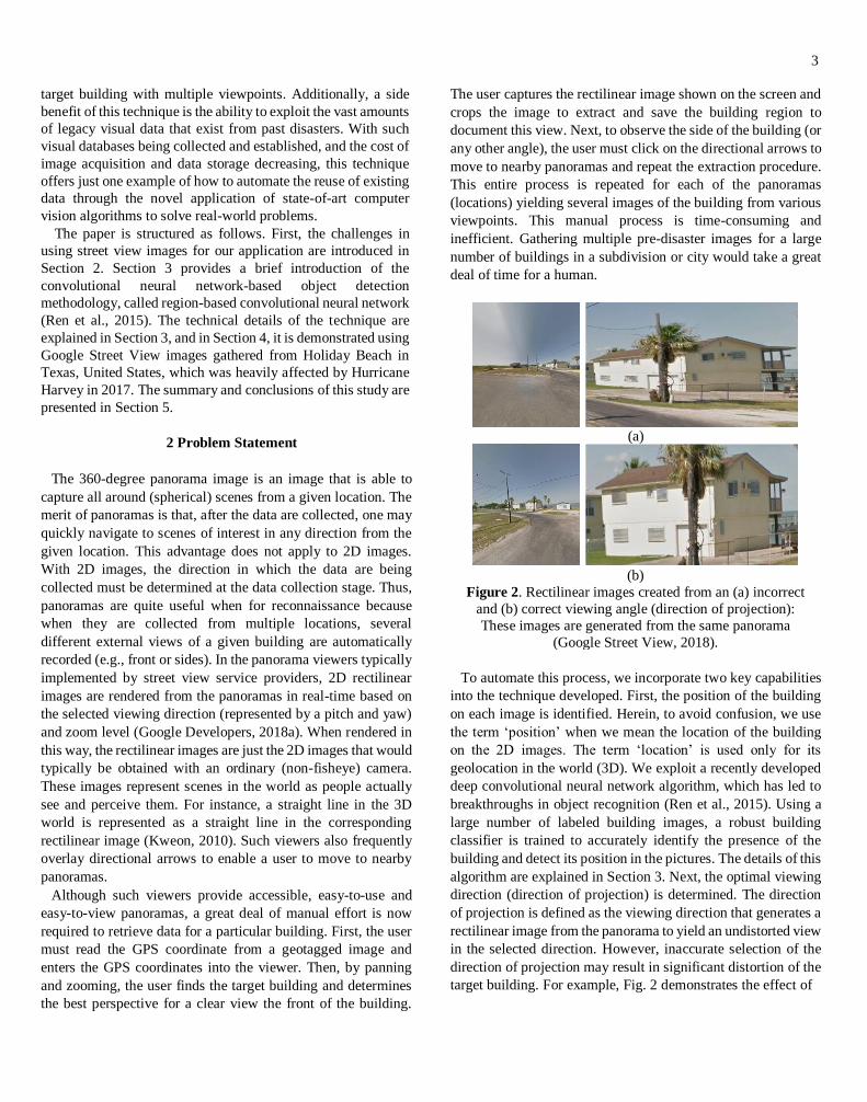
(a)

(b)

Figure 2. Rectilinear images created from an (a) incorrect

and (b) correct viewing angle (direction of projection):

These images are generated from the same panorama

(Google Street View, 2018).

To automate this process, we incorporate two key capabilities

into the technique developed. First, the position of the building

on each image is identified. Herein, to avoid confusion, we use

the term ‘position’ when we mean the location of the building

on the 2D images. The term ‘location’ is used only for its

geolocation in the world (3D). We exploit a recently developed

deep convolutional neural network algorithm, which has led to

breakthroughs in object recognition (Ren et al., 2015). Using a

large number of labeled building images, a robust building

classifier is trained to accurately identify the presence of the

building and detect its position in the pictures. The details of this

algorithm are explained in Section 3. Next, the optimal viewing

direction (direction of projection) is determined. The direction

of projection is defined as the viewing direction that generates a

rectilinear image from the panorama to yield an undistorted view

in the selected direction. However, inaccurate selection of the

direction of projection may result in significant distortion of the

target building. For example, Fig. 2 demonstrates the effect of

4 Lenjani et al.

projection direction on rectilinear images. Both sets of images

are generated from the same panorama. When the target building

is located further from the center of a rectilinear image, its

quality is degraded due to a large distortion. Thus, the most

suitable direction of projection of each panorama should be

determined to generate the 2D rectilinear image with the best

available quality. The implementation of this capability is

presented in Section 3.

3 Methodology

The technique developed herein is explained in Fig. 3. The

details are as follows. Users provide a geotagged image of the

target building (which includes the GPS coordinate near that

target building) and the input, and several images of the

corresponding building are automatically extracted from street

view images and the outputs. The resulting images contain

views of the building acquired from various viewpoints and

with negligible distortion. This technique will enable the user

to readily examine images of the entire front and sides of the

building in its pre-event condition.

The overall technique is divided into four main processes:

Steps 1 and 2 (captioned in light blue) download all panoramas

acquired near the target building from the street view service.

Steps 3 to 8 (captioned in dark blue) approximate the building

location in the GPS coordinate system using the geometric

relationship between the building and the panoramas.

Rectilinear images are generated from a couple of the closest

panoramas, and the trained building detector is applied to find

the building position on the rectilinear images. Then, the

location of the building is identified in each of the camera

coordinate systems, and transformed into the GPS coordinate

system. Note that this intermediate step is not yet intended to

extract high-quality building images because the rectilinear

images are generated without considering the optimal direction

of rectilinear projection. Steps 9 to 10 (captioned in green) are

generate the rectilinear image from each of the panoramas by

considering its optimal direction of projection. Lastly, Steps 11

to 12 (captioned in purple) detect the target building in each of

the optimal rectilinear images using the same building detector

and extract the building images for the final use. Again, once a

geotagged image is provided in Step 1, the rest of the process is

fully automated. The details of each step are provided below:

In Step 1, the GPS coordinate near the target building

(hereafter, the input GPS coordinate) is obtained from the EXIF

metadata of the input geotagged image(s) (Google Maps, 2018).

Note that this image is only needed for providing the GPS

information near the target building and thus, its quality or

visual contents do not affect this technique. Alternatively, a user

may manually provide approximate GPS information for the

target building.

Figure 3. Overview of the technique developed

5

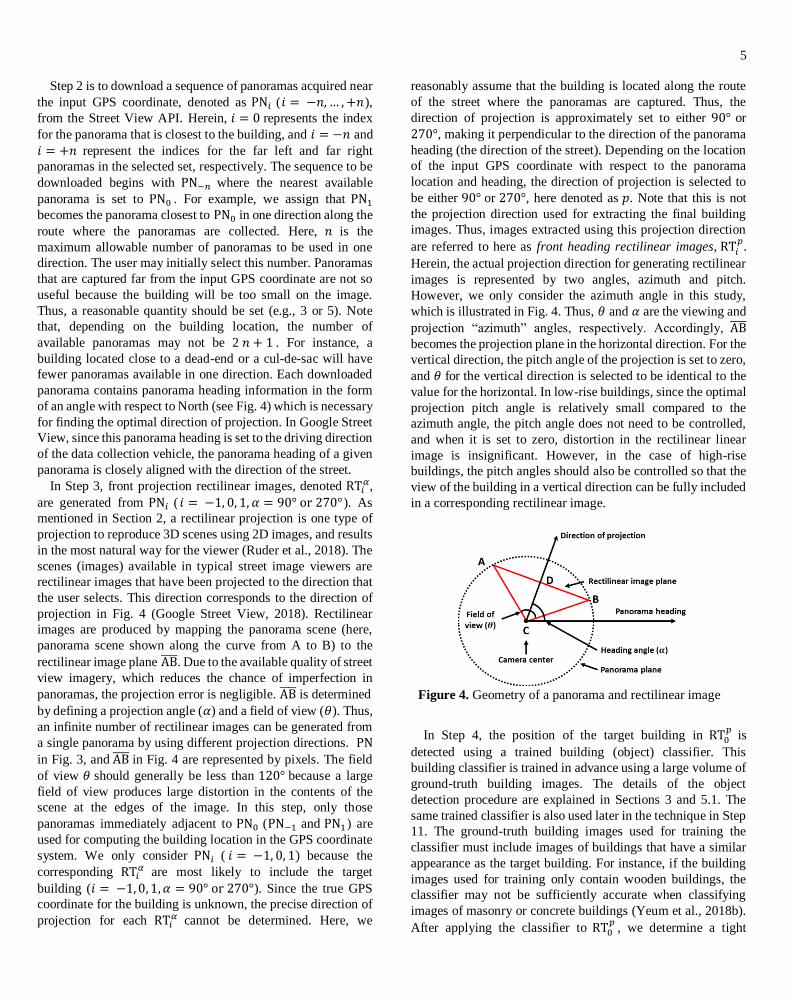
Step 2 is to download a sequence of panoramas acquired near

the input GPS coordinate, denoted as PN𝑖 (𝑖 = −𝑛, … , +𝑛),

from the Street View API. Herein, 𝑖 = 0 represents the index

for the panorama that is closest to the building, and 𝑖 = −𝑛 and

𝑖 = +𝑛 represent the indices for the far left and far right

panoramas in the selected set, respectively. The sequence to be

downloaded begins with PN−𝑛 where the nearest available

panorama is set to PN0 . For example, we assign that PN1

becomes the panorama closest to PN0 in one direction along the

route where the panoramas are collected. Here, 𝑛 is the

maximum allowable number of panoramas to be used in one

direction. The user may initially select this number. Panoramas

that are captured far from the input GPS coordinate are not so

useful because the building will be too small on the image.

Thus, a reasonable quantity should be set (e.g., 3 or 5). Note

that, depending on the building location, the number of

available panoramas may not be 2 𝑛 + 1 . For instance, a

building located close to a dead-end or a cul-de-sac will have

fewer panoramas available in one direction. Each downloaded

panorama contains panorama heading information in the form

of an angle with respect to North (see Fig. 4) which is necessary

for finding the optimal direction of projection. In Google Street

View, since this panorama heading is set to the driving direction

of the data collection vehicle, the panorama heading of a given

panorama is closely aligned with the direction of the street.

In Step 3, front projection rectilinear images, denoted RT𝑖𝛼,

are generated from PN𝑖 ( 𝑖 = −1, 0, 1, 𝛼 = 90° or 270° ). As

mentioned in Section 2, a rectilinear projection is one type of

projection to reproduce 3D scenes using 2D images, and results

in the most natural way for the viewer (Ruder et al., 2018). The

scenes (images) available in typical street image viewers are

rectilinear images that have been projected to the direction that

the user selects. This direction corresponds to the direction of

projection in Fig. 4 (Google Street View, 2018). Rectilinear

images are produced by mapping the panorama scene (here,

panorama scene shown along the curve from A to B) to the

rectilinear image plane AB̅̅ ̅̅ . Due to the available quality of street

view imagery, which reduces the chance of imperfection in

panoramas, the projection error is negligible. AB̅̅ ̅̅ is determined

by defining a projection angle (𝛼) and a field of view (𝜃). Thus,

an infinite number of rectilinear images can be generated from

a single panorama by using different projection directions. PN

in Fig. 3, and AB̅̅ ̅̅ in Fig. 4 are represented by pixels. The field

of view 𝜃 should generally be less than 120° because a large

field of view produces large distortion in the contents of the

scene at the edges of the image. In this step, only those

panoramas immediately adjacent to PN0 (PN−1 and PN1) are

used for computing the building location in the GPS coordinate

system. We only consider PN𝑖 ( 𝑖 = −1, 0, 1) because the

corresponding RT𝑖𝛼 are most likely to include the target

building (𝑖 = −1, 0, 1, 𝛼 = 90° or 270°). Since the true GPS

coordinate for the building is unknown, the precise direction of

projection for each RT𝑖𝛼 cannot be determined. Here, we

reasonably assume that the building is located along the route

of the street where the panoramas are captured. Thus, the

direction of projection is approximately set to either 90° or

270°, making it perpendicular to the direction of the panorama

heading (the direction of the street). Depending on the location

of the input GPS coordinate with respect to the panorama

location and heading, the direction of projection is selected to

be either 90° or 270°, here denoted as 𝑝. Note that this is not

the projection direction used for extracting the final building

images. Thus, images extracted using this projection direction

are referred to here as front heading rectilinear images, RT𝑖𝑝.

Herein, the actual projection direction for generating rectilinear

images is represented by two angles, azimuth and pitch.

However, we only consider the azimuth angle in this study,

which is illustrated in Fig. 4. Thus, 𝜃 and 𝛼 are the viewing and

projection “azimuth” angles, respectively. Accordingly, AB̅̅ ̅̅

becomes the projection plane in the horizontal direction. For the

vertical direction, the pitch angle of the projection is set to zero,

and 𝜃 for the vertical direction is selected to be identical to the

value for the horizontal. In low-rise buildings, since the optimal

projection pitch angle is relatively small compared to the

azimuth angle, the pitch angle does not need to be controlled,

and when it is set to zero, distortion in the rectilinear linear

image is insignificant. However, in the case of high-rise

buildings, the pitch angles should also be controlled so that the

view of the building in a vertical direction can be fully included

in a corresponding rectilinear image.

Figure 4. Geometry of a panorama and rectilinear image

In Step 4, the position of the target building in RT0𝑝

is

detected using a trained building (object) classifier. This

building classifier is trained in advance using a large volume of

ground-truth building images. The details of the object

detection procedure are explained in Sections 3 and 5.1. The

same trained classifier is also used later in the technique in Step

11. The ground-truth building images used for training the

classifier must include images of buildings that have a similar

appearance as the target building. For instance, if the building

images used for training only contain wooden buildings, the

classifier may not be sufficiently accurate when classifying

images of masonry or concrete buildings (Yeum et al., 2018b).

After applying the classifier to RT0𝑝

, we determine a tight

6 Lenjani et al.

bounding box for the building in that image. If more than one

building is detected in RT0𝑝, the bounding box that is closest to

the center of RT0𝑝

is selected, denoted as 𝑏𝑏𝑜𝑥0 (the

subscription indicates the order, or index, of the image).

Step 5 is to extract and match the visual features between

RT𝑖𝑝 (𝑖 = −1, 0, 1). The features extracted from RT0

𝑝 must be

matched with the corresponding features from RT−1𝑝

and RT1𝑝.

Conventional visual features and descriptors (e.g., SIFT or

SURF) can be used for this process (Lowe, 2004). These visual

features and their descriptors represent unique key points across

the images and are used for computing the geometric

relationship (essential matrix in this study) between images.

Then, a single rectilinear image is selected from either RT−1𝑝

or

RT1𝑝

, which is chosen as the one with the larger number of

matched features, denoted as RT𝑐𝑝. This process is intended to

improve the accuracy of building location estimation by using

more information. For example, the building on RT0𝑝 is often

shifted slightly because the input GPS coordinate may not be

recorded at the location of the panorama closest to the house. In

such a case, either RT−1𝑝

or RT1𝑝 may be far from the panorama

closest to the building, and the other panorama is unlikely to

include the same building, causing a failure in estimating the

building location. Unless the building is far from the street

along which the panoramas were captured, the building often

occupies a large portion of each image, and thus many features

generated from the building regions will be matched. One of

these features that is close to the center of 𝑏𝑏𝑜𝑥0 will be used

for computing the building location in Step 7.

In Step 6, the projection matrices of RT0𝑝

and RT𝑐𝑝

are

computed. The projection matrix is a 3×4 matrix which

represents the mapping from 3D points in the world to 2D points

in an image. In this study, the projection matrices of RT0𝑝 and

RT𝑐𝑝

are computed using an essential matrix between two

images, and the corresponding projection matrices are denoted

as 𝑃0 and 𝑃𝑐 in (see Fig. 3), respectively. The essential matrix is

a special case of a fundamental matrix for which the intrinsic

(calibration) matrix for both cameras is known (Hartley and

Zisserman, 2003). Using the panorama’s geometry in Fig. 3, the

intrinsic matrix having principal points and a focal length is

obtained, and it is identical for both RT0𝑝 and RT𝑐

𝑝. Since the

essential matrix has only five degrees of freedom to be

estimated from RT0𝑝 and RT𝑐

𝑝, fewer degrees of freedom than

the fundamental matrix, more accurate projection matrices can

be computed. Based on the pairs of visual feature matches in

Step 5, the essential matrix is estimated using the five-point

algorithm combined with RANSAC (RAndom SAmple

Consensus) (Fischler and Bolles, 1981; Nister, 2004). For the

mathematical representation of this process, the intrinsic matrix

(𝐾) is represented as:

0 0

0 0

0 0 1 0 0 1

=

x x

y y

f p f p

K f p f p=

,

(1)

where 𝑓 and 𝑝 are the focal length and the coordinates of the

principal point, and the subscripts 𝑥 and 𝑦 indicate the width

and height directions, respectively. Since we consider the same

viewing angle in the horizontal and vertical directions, so 𝑓𝑥

and 𝑓𝑦 (and 𝑝𝑥 and 𝑝𝑦) are the same regardless of the direction.

In Fig. 4, CD̅̅ ̅̅ and AD̅̅ ̅̅ (= BD̅̅ ̅̅ ) are 𝑓 and 𝑝, respectively. Thus,

𝑓 becomes:

arctan( / 2)= f p, (2)

where 𝑝 is half of the size of the rectilinear image in pixels,

meaning that the principal point is the center of the rectilinear

images. The pairs of matched feature points are transformed by

multiplying the inverse of 𝐾 by their points coordinates (in the

homogeneous coordinate system). Then, those points are

expressed in a normalized coordinate system, denoted as x0 in

RT0𝑝 , and x𝑐 in RT𝑐

𝑝 (Hartley and Zisserman, 2003). The

essential matrix (𝐸) satisfies the following relationship:

0x x 0=T

c E.

(3)

The five-point algorithm based on this relationship is utilized

as a hypothesis-generator (model) for RANSAC to count the

number of inliers and outliers, and the inliers are used for

estimating 𝐸 (Hartley and Zisserman, 2003; Li and Hartley,

2006). The estimated 𝐸 enables us to extract 𝑃𝑐 if 𝑃0 is assumed

to be a canonical projection matrix (𝑃0 = [I 0] where I is a 3

× 3 identity matrix) (Hartley and Zisserman, 2003). In this case,

the origin of the camera coordinate system is the camera center

(focal point) of RT0𝑝(generated from PN0).

In Step 7, the approximate 3D locations of the building are

identified in the camera coordinate system. When the direction

of projection is generally aimed toward the center of the

building façade, distortion on the rectilinear images can be

minimized. Given the projection matrices 𝑃0 and 𝑃𝑐 , we can

compute the 3D points in the camera coordinate system that

correspond to a pair of matched image points (point

correspondence) using a linear triangulation algorithm (Hartley

and Zisserman, 2003). From Steps 4 and 5, we have a set of

matched image points between RT0𝑝

and RT𝑐𝑝

. However, the

visual features and/or the matched sets are randomly distributed

over the building region on those images, and thus it is not

guaranteed that we will obtain the exact center of the building

façade. Moreover, depending on the locations of PN0 and PN𝑐

with respect to the building and the width of the building, they

may include a portion of the side of the building, meaning that

the center of the bounding box may not be the center of the

building façade. Thus, we reasonably define the 3D building

location (in the camera coordinate system) as the 3D point

generated from the matching feature closest to the 𝑏𝑏𝑜𝑥0. Once

7

we find the matching feature nearest to this point, its

corresponding location in 3D space is identified in the GPS

coordinate system. The estimated building location is denoted

as 𝑋𝐵.

Step 8 is to perform a 2D similarity transformation to define

𝑋𝐵 in the GPS coordinate system, denoted as 𝑋𝐺. In Step 2, each

of the panoramas downloaded from street view services has its

own accurate GPS information (Google Maps, 2018) and the

3D locations of PN0, PN𝑐, and 𝑋𝐵 are computed in the camera

coordinate system using Steps 3~7. However, these two control

points (the same points in two different coordinate systems) are

not entirely sufficient to compute a 3D similarity transformation

between the two coordinate systems (Horn, 1987). Since the

positions of the camera when it is acquiring the data

(panoramas) are almost co-linear (because the street view

vehicle is driving along a street), adding one additional control

point by considering another (3rd) camera location does not add

a new equation to obtain a unique transformation. Alternatively,

we choose to eliminate one of the dimensions in both coordinate

systems. Because the panoramas are captured from a street view

vehicle, the camera acquiring the panoramas moves along a

path that is almost entirely in a single plane with a consistent

height (negligible street slope exists between two panorama

locations) in the camera coordinate system. Accordingly, we

can assume that the variation in the camera’s altitude in the GPS

coordinate system is minimal and can be ignored. With two

pairs of camera locations in both the camera coordinate system

(considering only the image width and depth directions) and the

GPS coordinate system (considering only latitude and

longitude), we have a sufficient number of equations to perform

the 2D similarity transformation using the two translational,

two rotational, and one scaling parameters that are available.

Here, the camera location in PN0 is [0 0 0] and PN𝑐

becomes −M−1𝑝4 where M is the left 3 × 3 submatrix of 𝑃𝑐 and

𝑝4 is the last column of 𝑃𝑐 (Hartley and Zisserman, 2003). GPS

coordinates are typically recorded in geodetic coordinates

(represented as longitude and latitude). Note that this system is

not a Euclidean space, as the one used in the camera coordinate

systems. The geodesic datum should thus be represented by the

equivalent values in Euclidean space (Drake, 2002). Since the

distance between the two panoramas is relatively small

compared to the radius of the Earth, we can use the flat Earth

assumption in which the values are transformed into an Earth-

north-up (ENU) coordinate system (Pandey et al., 2011). The

ENU coordinates are formed from a plane tangent to a fixed

point on the Earth’s surface. Coordinates of the points are found

by computing translational movements on the tangential plane

to East (X) and North (Y) from the fixed point. Then, finally,

we can identify the 2D similarity transformation matrix using

these two pairs of control points defined in two different

Euclidian coordinate systems. The transformation matrix is then

applied to 𝑋𝐵 to obtain 𝑋𝐺.

In Step 9, the correct projection directions for PN𝑖 ( 𝑖 = −𝑛, … , +𝑛) are computed to generate the optimal rectilinear

images. PN𝑖 have the panorama heading with respect to North,

and their locations are defined in the ENU coordinate system

obtained in Step 8. Thus, as shown in Step 9 in Fig. 3, the

correct projection directions (𝛼𝑖) can be computed.

In Step 10, RT𝑖𝛼𝑖 are generated from PN𝑖 using 𝛼𝑖 computed

in Step 9 (𝑖 = −𝑛, … , +𝑛), and these are the optimal rectilinear

images. This step repeats the same process in Step 3 for all

panoramas, although at this point the process is performed using

the correct projection angles. Since the projection direction is

aimed toward the target building, the target building is now at

the center of each RT𝑖𝛼𝑖.

In Step 11, the position of the target building in each RT𝑖𝛼𝑖 is

detected using the trained building classifier, which is identical

to the classifier used in Step 4. The only difference compared

to Step 4 is that here we detect the building within the optimal

rectilinear images generated from all panoramas, which contain

undistorted views of the target building.

Finally, in Step 12, we obtain the set of highly localized target

building images captured from various viewpoints. The

detected target building images having various viewpoints are

cropped from RT𝑖

𝛼𝑖 , which are captured from different

locations.

In our study, the visual recognition (Papageorgiou et al.,

1998; Viola and Jones, 2004; Dalal and Triggs, 2005) of the

building is used both for estimating its 3D location by

computing the geometric relationship between the panoramas

(Step 4 in Fig. 3) and for detecting and cropping its region on

each rectilinear image (Step 11 in Fig. 3). Accurate detection

and positioning of each building on the images are critical for

achieving the successful extraction of pre-event building images

from the panoramas. Recently several CNN based high

performance object detection algorithms have been presented

(Girshick et al., 2015; Ren et al., 2015; Redmon and Farhadi,

2017). We incorporate a state-of-art object detection method,

called faster region-based convolutional neural network (Faster-

RCNN) into our technique (Ren et al. 2015; 2017). Faster-

RCNN is an evolved version of region-based convolution neural

network in terms of speed and accuracy (Harzallah et al., 2009;

Hinton and Salakhutdinov, 2009; Uijlings et al., 2013; Girshick

et al., 2014; Chen et al., 2015; Girshick, 2015; LeCun et al.,

2015; Krizhevsky et al., 2017). Recently, an enhanced version

of Fast R-CNN, in terms of speed and accuracy. Many other

architectures have been introduced to reduce the training and

testing speed as well as the accuracy, but there is always a trade-

off between the accuracy and computational efficiency (Liu et

al.,2016; Redmon and Farhadi, 2017). In this study, we

implement the original Faster R-CNN to detect buildings on the

images.

To close this section, we comment on some assumptions used

in the technique that one must remember for successful

implementation. First, of course, the panoramas used must

8 Lenjani et al.

contain the target building. Updates on the panoramas in the

street view are infrequent in remote areas, and this highly

depends on the location (i.e., urban or rural regions), although

data collection is generally increasing in frequency. Recently

constructed buildings may not be captured in the panoramas,

and renovated buildings may not always have up-to-date

images. One possible solution is to explore various street view

services as their data collection periods and frequencies are

different. Second, the geotagged image used as the input to the

technique should be collected from a location near the target

building. The GPS coordinates stored in the metadata should be

close to the target building. Recall that the actual visual contents

of this input image is not actually used in the technique, and its

quality is not relevant. However, it is recommended that each

post-disaster geo-tagged image include only one building to

prevent confusions while comparing the images with pre-

disaster images. For example, if the input image is acquired

from a location that is closer to a different building, images of

the wrong building may be generated. Third, the technique

relies highly on the availability and accuracy of information in

the street view service used. Here the panoramas and related

metadata are directly obtained from street view services. If such

information has limited availability or it is not accurate, the

results will be incorrect. For example, incomplete or erroneous

GPS coordinates for the panoramas would yield the wrong a

building location, followed by erroneous projection direction

estimation. However, GPS data is generally accurate enough for

this purpose, and we have not observed any errors in the data to

date. Although we successfully demonstrate the technique using

Google Street View, we have not tested it using panoramas

available through the other street view services. Fourth, the

panoramas acquired must have sufficient spatial coverage

(roughly not more than 10 meters). If the distance between

adjacent panoramas is too far to contain the same target

building, the technique will fail to correctly estimate the

location of the building in Steps 3 to 6. Moreover, such sparse

panoramas hinder the goal to obtain several high-quality

building images. Fifth, there should be a reasonable distance

between the panoramas and the building, enough to ensure that

the panorama does exclusively contain the building in a

rectilinear image. Since most of the panoramas are captured

along the street, their distances from the building are often

sufficiently far from the target building (e.g., more than the

width of a single lane). However, when the distance between

the buildings and the panorama location and/or their height or

width are large, a greater FOV is needed to capture the entire

view of the building. This limitation would cause a large

distortion in the rectilinear images.

4 Experimental Validation

4.1 Description of the test site

To demonstrate the performance of the technique, we use

residential buildings in Holiday Beach in Rockport, Texas as

(a) (b)

Figure 5. Test site for experimental validation, Holiday

Beach: (a) Geolocation of Holiday Beach on a map and a

selected path used for constructing house image database

and (b) Samples of damaged residential buildings in

Holiday Beach after Hurricane Harvey in 2017 (Metz,

2017).

our case study. Hurricane Harvey in 2017 is the second-most

costly hurricane in U.S. history, inflicting $125 billion in

damage, primary due to catastrophic rainfall-triggered flooding

in the Houston metropolitan area (Smith, 2018). Harvey made

landfall as a Category 4 Hurricane in southern Texas, and

Rockport was directly in the path of Harvey, causing

tremendous wind and storm surge damage (Metz, 2017).

Holiday Beach, shown in Fig. 5(a), is a residential community

and most of its residential buildings (more than 80%) (hereafter,

houses) in the region were substantially damaged (Villafranca,

2017).

Several reconnaissance teams were dispatched to these

regions in the weeks and months after the event to evaluate

structures, characterize the event, and collect data to learn from

this event (FEMA, 2018). Several such teams published their

data through designsafe-ci.org and weather.gov (Metz, 2017;

Stark and Wooten, 2018). Geotagged images collected from

Holiday Beach are also available, the selection of sample

images shown in Fig. 5(b) highlights the need for observing

their pre-disaster condition. It is evident that when presented

with such photos of severely damaged houses, little information

is available to identify the vulnerabilities that may have existed.

Here, these post-disaster reconnaissance images are the input to

the technique and are used solely for providing GPS coordinates

to automate the process of extracting useful photos of the target

houses.

(a) (b)

Figure 6. Sample panorama in (a) and the corresponding

optimal rectilinear image in (b) for a target house

9 Lenjani et al.

Figure 7. Sample building images used for training a residential building (house) classifier.

4.2 Construction of residential building image database

A large volume of ground-truth house images is prepared to

train a residential building classifier using the algorithm

discussed in Section 3. The house images used for this training

process should be similar in appearance (architecture style) to

those expected for actual testing and implementation. For

instance, our goal here is to detect wooden residential buildings

for single family residence. Wood is a standard construction

material for houses across the Southern part of the United

States. Training a classifier using images of high-rise

apartments or concrete buildings would not improve its

performance unless those are expected to be present in the

images collected from the testing and implementation regions.

For simplicity, we prepare our ground-truth training images

using representative scenes from Holiday Beach to ensure the

buildings have similar styles and appearances. The distribution

of the buildings used in the ground-truth dataset is quite similar

to the appearance of houses across the other coastal areas of the

United States. To prepare the training images for the classifier,

we exploit Steps 1 to 10 from the technique developed to

generate a large volume of optimal rectilinear images. Then, we

manually label that large volume of images to construct our

ground-truth residential building database. Note that the

resulting residential building classifier is generally applicable,

and is trained in advance for use across many events and

regions. The database can also be expanded over time to

encompass other building types, materials, architecture and

styles.

First, panoramas along the selected route on the waterfront in

Fig. 5a (marked a red line) are downloaded from Google Street

View. Google Street View does not provide a service to directly

download high-resolution panoramas, but does have an API to

download (show) a portion of the panorama when the user

specifies a horizontal and vertical position and a size (Google

Developers, 2018a; Google Developers, 2018b; Google

Developers, 2018c). The tool that we developed automatically

downloads the tiles of each panorama and stitches them together

to generate high-resolution panoramas. The resolution of each

panorama is 13,312 × 6,656 pixels. Each panorama is

constructed by stitching 338 tiles having a resolution of 512 ×

512 pixels. A total of 128 panoramas are available along these

routes. A sample of a high-resolution panorama is shown in Fig.

6(a). Second, we manually select the GPS locations of many of

the houses along the chosen route in Fig. 5(a). A footprint

(outline) of each house can be viewed in Google Maps, and thus,

its GPS location can be easily obtained. 100 houses are

considered along the route having similar house styles (e.g.,

number of floors, roof style, elevated house foundation). Note

that for constructing the ground-truth database, this manual

process is necessary and replaces the geotagged images that

would be used in the implementation of the technique following

Steps 3 to 8.

Third, optimal rectilinear images are generated from the

downloaded panoramas. Since here we know the GPS

coordinates of each of the downloaded panoramas as well as the

houses, the optimal projection angles can be directly computed.

Here, 𝑛 is set to be five, which is the maximum allowable

number of images on one side of the closest panorama location.

Thus, for each house, a maximum of 11 rectilinear images are

constructed from the corresponding panoramas (houses at a

dead-end along the route would have fewer than 11 panoramas),

and each house is positioned at the center of each of the

rectilinear images. 𝜃 and 𝐴𝐵̅̅ ̅̅ are 120° and 2,048 pixels,

respectively. As a result, a total of 1,056 rectilinear images

having a resolution of 2,048 × 2,048 pixels are generated for the

database. Figure. 6(b) shows the optimal rectilinear image

generated from the sample panorama in Fig. 6(a).

Finally, the houses on the rectilinear images are manually

labeled. We used a Python-based open source labeling tool to

label a tight bounding box around each house (Tzutalin, 2015).

Only houses that satisfy the following two conditions are

labelled: (1) less than 70% of the front and side views of the

house are obstructed by foreground objects, and (2) the height

or width of the bounding box encompassing each house is larger

than 200 pixels, which is around a tenth of the rectilinear image

size in pixels. Samples of labeled houses are shown in Fig. 7.

Here, only bounding boxes with solid blue lines are labeled as

a house, while the other houses in these images are not included

as ground-truth data. Those houses are marked with a red dotted

line purely for purposes of illustrating non-labeled house data.

The left image in Fig. 7, the red dotted bounding box around the

10 Lenjani et al.

(a) (b)

Figure 8. The performance of the residential building detector for the testing set: (a) PR curve and (b) ROC curve.

Figure 9. Samples of detected residential buildings using Faster R-CNN algorithm.

house on the left has height less than 200 pixels, and thus it does

not contain sufficient information for our purpose. Similarly, in

the right image in Fig. 7(b), all non-labeled houses are

obstructed by the foreground objects (e.g., vehicle, tree, or other

house) or are only partially visible. A total of 3,500 ground-truth

residential buildings are labeled from the rectilinear images, and

this database is utilized for training the classifier.

4.3 Training and testing residential building detector

11

An open-source library of Faster R-CNN deployed using

Python is used for training and testing the residential building

detector (Chen and Gupta, 2017). A single NVIDIA Tesla K80

is used for this computation. A total number of 3,500 residential

houses have been labeled from 1,050 images. This set includes

different views of 100 houses in Holiday Beach. Sets containing

60%, 10%, and 30% of the images of target houses are randomly

chosen as training, validation, and testing sets, respectively. The

Residual Network Model (called ResNet_101) is selected for

learning robust features and increasing its efficiency (He et al.,

2016). We manually chose the hyper-parameters for Faster R-

CNN based on trial-and-error. Then, the ConvNets and Fully-

connected layers are initialized by zero-mean Gaussian with

standard deviations of 0.01 and 0.001, respectively.

Hyperparameters including learning rate, momentum and

weight decay for training R-CNN and RPN networks are set to

0.001, 0.9, and 0.0005, respectively. The learning rate is defined

as the amount the weights are adjusted with respect to the loss

gradient. The decay weight is set to avoid overfitting by

decaying the weight proportionally with its size. We set the

momentum to 0.9 to make the gradient decent achieve a faster

convergence. We used three different aspect ratios (0.5, 1, and

2) and anchor sizes (128, 256, and 512 pixels). In the test stage,

in cases in which a set of the detected proposals that overlap

each other with greater than a 0.3 intersection over union (IoU),

an additional process is needed to obtain a precise bounding

box. In each set, the proposal having the highest confidence

score (probability) remains, and the others are disregarded. This

process is called non-maximum suppression. Then, a threshold

is set to keep only proposals having high confidence scores. In

this study, this threshold is set to 0.5.

We evaluate the performance of the trained residential

building detector using the testing image set. Precision-recall

(PR) and receiver operating characteristic (ROC) curves are

used to evaluate the performance of the classifier quantitatively.

To construct the PR curve, each detection first maps to its most

overlapping ground-truth object samples. In this study, the

threshold for considering a detection as successful is defined as

an overlap of more than 50% IoU. True positive is defined as a

detection with the highest-score (probability) mapped to each

ground-truth sample, and all other detections are considered as

false-positives. Precision is defined as the proportion of true

positives to all detections. Recall is the proportion of the true

positives to total number of ground-truth samples. Plotting the

sequence of precision and recall values yields the PR curve

shown in Fig. 8(a). The typical method to evaluate the

performance of the object detector is to calculate the average

precision (AP) (Girshick et al., 2014; Ren et al., 2015), which is

the area under the PR curve (Everingham et al., 2010). The

results show an AP of 85.47 % for the single class of residential

house detection. An ROC curve, which represents the

relationship between sensitivity (recall) and specificity (not

precision), is also used to evaluate the performance of the

detector. As mentioned previously, each detection is considered

to be positive if its IoU ratio with its corresponding ground-truth

annotation is higher than 0.5. By varying the threshold of

detection scores, a set of true positives and false positives will

be generated which is represented as the ROC curve. From Fig.

8(b), we can interpret this result to mean that the residential

building detector consistently achieves impressive performance

in terms of the ROC curve by obtaining true positive rates of

81.49% and 88.07% at 100 and 200 false positives, respectively.

Samples of detected houses using the optimal rectilinear

images are shown in Fig. 9. Figures 9(a) and (b) shows typical

successful cases in which all bounding boxes are correctly

detected and tightly encompass each of house areas. Figures

9(c), (d), (e) and (f) show more challenging cases, which likely

produce incorrect results. These results can be polished by

adjusting the parameters used in the technique. Figures. 9(c) and

(d) show two particular images which, in addition to correctly

detecting houses, erroneous objects are also detected as a house.

Figure. 9(c) demonstrates a case in which a boat is detected as

a house with a score of 0.779. Also, in Fig. 9(d) a cargo trailer

is detected as a house with a score of 0.571 which is not of

interest in this study. As illustrated, all incorrect detections yield

a low score, less than 0.8, which enables us to simply remove

them using a higher threshold value for positive detection. Since

in our application the target house is only likely to appear close

to the center of the optimal rectilinear image, the target house

would be detected with a high score, usually more than 0.95,

unless either the image was captured far from the target house,

or obstacles conceal the target house. Therefore, the problem of

erroneous detections can be remedied by merely increasing the

confidence threshold, here 0.8, to retain only the objects that

receive a high score.

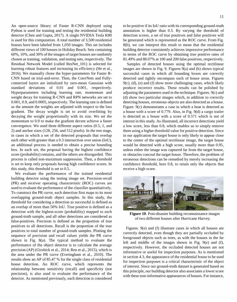
Figure 10. Post-disaster building reconnaissance images

of two different houses after Hurricane Harvey.

Figures. 9(e) and (f) illustrate cases in which all houses are

correctly detected, even though they are partially occluded by

foreground objects such as trees, as with the houses in the far

left and middle of the images shown in Fig. 9(e) and (f),

respectively. However, the occluded detected houses are not

informative or useful for inspection purposes. As is mentioned

in section 4.3, the appearance of the residential house to be used

for inspection purposes is a critical characteristic of the object

of interest. Since our ground-truth dataset is generated based on

this principle, our building detector also associates a lower score

with these non-informative appearances of houses. For instance,

12 Lenjani et al.

the occluded houses shown in Fig. 9(a) and (b) are detected with

scores of 0.839 and 0.507, respectively, which are considerably

lower than the non-occluded houses appearing in these images.

Although these objects are correctly detected as a house, the

images are not useful for inspection purposes. Considering the

fact that we extract several (here, 11) optimal rectilinear images

for each target house, every image need not be informative for

inspection, and we can safely increase the confidence threshold

to remove those non-informative house detections.

4.4 Sample implementation

In this section, the implementation of the technique

developed is demonstrated using real-world post-event

reconnaissance geotagged images collected from Holiday

Beach, Texas after Hurricane Harvey in 2017. Pre-disaster

images of two selected houses are automatically generated from

the corresponding geotagged post-disaster images in Fig. 10.

The house in Fig. 10(a) is merely a shell gutted by the hurricane

and its appearance before the hurricane is hard to guess. The

house on the right in Fig. 10(b) has significant shingle damage

on the roof. One additional house is added, which does not have

a geotagged image. The approximated GPS information near

that second house is manually provided, rather than through a

geotagged image. The locations of these houses are along the

selected route in Fig. 5(a). All pre-disaster images for these

three different houses are automatically generated using the

technique developedThe proposed approach incorporates

several program libraries including OpenCV (Bradski, 2000)

and PyMap3D (Hirsch, 2018), and an implementation Faster R-

CNN algorithm in TensorFlow (Chen and Gupta, 2017), and is

deployed as a Python script. For this testing, we utilize the same

computing resources to run this script, which are used for

training the house classifier. For setting up the parameters

introduced in Section 3, 𝑛 is set to five, so the maximum

number of house images available is 11. 𝜃 and 𝐴𝐵̅̅ ̅̅ are 90° and

2,048 pixels, respectively, which are the same as those used for

generating training images. With this setup, at each house, the

approximate processing time for conducting the four main

processes explained in the first paragraph of Section 3 are

approximately 130, 210, 180 and 6 seconds, respectively. As

mentioned in Section 4.2, high-resolution panoramas cannot be

downloaded from Google Street Views directly. It takes a

considerable time to create each panorama by stitching an array

of the images. Unfortunately, this cannot be technically

addressed in the front-end software, unless in the near future

one is allowed to download panoramas from Google Street

View directly.

(a)

(b)

(c)

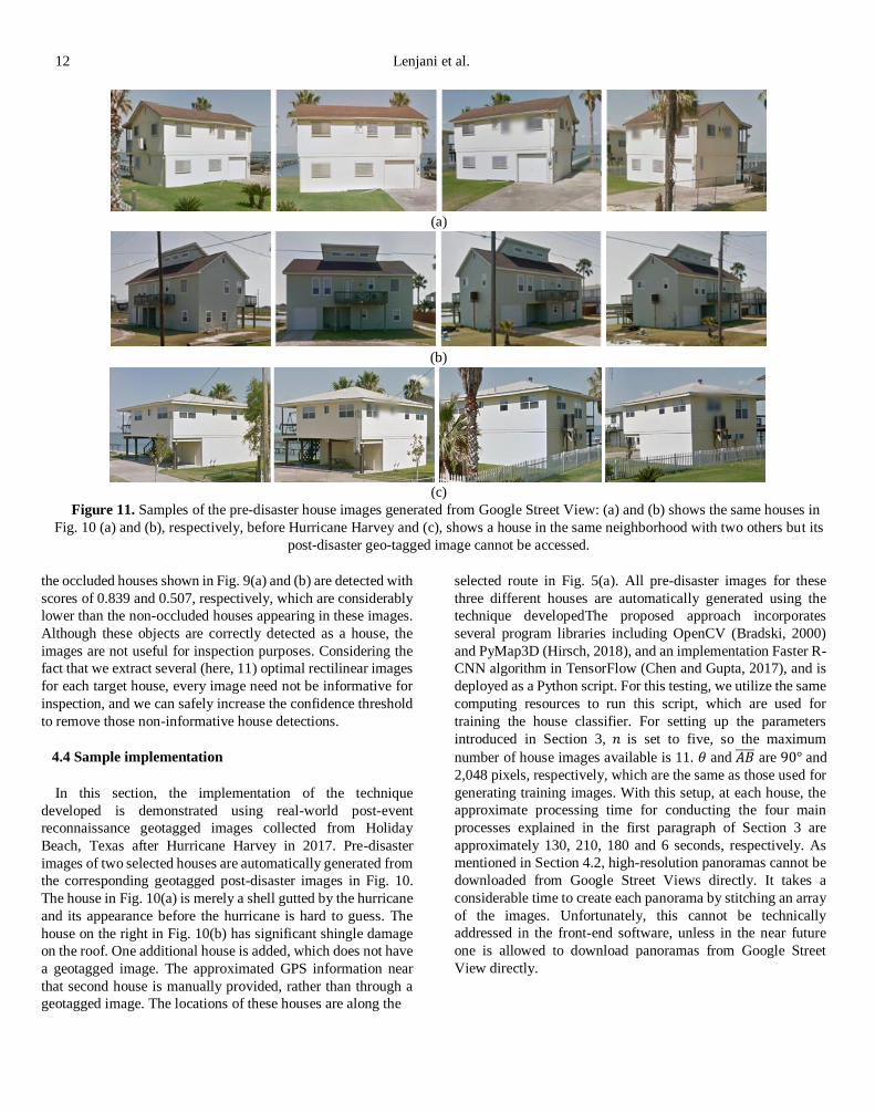
Figure 11. Samples of the pre-disaster house images generated from Google Street View: (a) and (b) shows the same houses in

Fig. 10 (a) and (b), respectively, before Hurricane Harvey and (c), shows a house in the same neighborhood with two others but its

post-disaster geo-tagged image cannot be accessed.

13 Lenjani et al.

Figure 12. Reason to observe the house from multiple viewpoints: Optimal rectilinear images with the bounding boxes of the

detected house from multiple views. Since the views of the house are partially or entirely obstructed by the foreground objects

(here, trees), many images from different viewpoints should be considered to observe the entire front and side views of the house.

However, the rest of the three processes are relatively fast and

can be potentially improved by exploiting better hardware or

optimizing the deployment of the Python scripts.

The results in Fig. 11 show the pre-disaster house images

automatically extracted from Google Street View using our

technique. Figures. 11(a) and (b) show the pre-event appearance

of the houses shown in Fig. 10(a) and (b), respectively, and Fig.

11(c) demonstrates the generation of pre-event images of the

same house without a post-event geo-tagged image. The seven

images of houses shown in Fig. 11(a) and (b) and the five

images of houses shown in Fig. 11(c), from various viewpoints

are detected from the 11 optimal rectilinear images, although

only four representative samples of those images are provided

in Fig. 11. It is clear from these samples that including images

of each house from multiple viewpoints is important for

enabling observation of the entire side and front façade of the

house. Clearly, they provide valuable information about the pre-

hurricane state of the house. For example, the pre-event

appearance of the house shown in Fig.11(a) can hardly be

imagined using only the post-disaster image in Fig. 10(a).

Figure 12 shows the six optimal rectilinear images generated

for the house in Fig. 11(c). The bounding box of the

corresponding house in each rectilinear image is marked. This

example further demonstrates why multiple images from

different viewpoints should be extracted (in other words, 𝑛

should be set to more than two). Since large trees in front of this

house block its view, multiple images are needed to observe the

entire view of the house. This situation commonly occurs in

cluttered scenes where various sources of foreground objects

are potentially present in a street view, for instance, large street

signs, parked vehicles, trees, or pedestrians. This issue can be

minimized by increasing 𝑛 to consider more viewpoints.

4.5 Technique validation

For further evaluation of the technique developed, we introduce

a new metric, denoted Overall Practicality (OP). In this

technique, the potential sources of error include: (1) incorrect

estimation of the GPS location of the building due to a feature

matching failure (Steps 3~ 8), (2) false building detection on the

rectilinear images using the trained classifier, and (3) incorrect

GPS records for the street view panoramas. The new metric,

𝑂𝑃 , is designed to quantitatively evaluate the likelihood of

extracting a sufficient set of building images of the quality of

the resulting images in Fig. 11. 𝑂𝑃 is formulated as:

𝑂𝑃 = 𝑁𝑢

𝑁𝑡 − 𝑁𝑜 , (4)

where, 𝑁𝑢 is the number of extracted images that contain a

satisfactory view of the target building on the corresponding

rectilinear images. When the extracted building is not placed

near the center of the rectilinear images, due to the projection

direction error, it does not contribute to 𝑁𝑢 although it contains

enough of the building’s appearance. Also, if the trained

classifier only detects a portion of the building or does not

tightly estimate its region with a bounding box, it is also not

included in 𝑁𝑢. 𝑁𝑡 is the number of all building images which

can be extracted from the available panorama. It can be

calculated as 𝑁𝑡 = 𝑁𝑏(2𝑛 + 1) − ∑ 𝑁𝑏𝑖=1 𝑚𝑖 , where 𝑁𝑏 is the

total number of target buildings, 𝑛 is the maximum allowable

number of images (see Section. 5.2), and 𝑚𝑖 is the number of

missing panoramas at building 𝑖 . As mentioned in Section 3

(Step 2), if a building is located close to a dead-end or a cul-de-

sac, street view panoramas are not available. 𝑁𝑜 is the number

of occluded images. The occlusion due to foreground objects

(e.g. tree, car, or fence) is inevitable, and can obstruct the view

14 Lenjani et al.

of the building. Thus, it is a clear basis for needing multi-view

images. This number is not contained in either 𝑁𝑢 or 𝑁𝑡.

To evaluate the performance of the technique developed

using 𝑂𝑃, we randomly select 50 residential buildings along a

different street (marked using a black line in Fig. 5(a)). In the

actual implementation, the input of the technique is a geo-tag

image which must be captured close to the building-of-interest.

However, existing data sets rarely have a sufficient number of

geo-tagged images available. Thus, in this evaluation, we

manually provide similar GPS information for each building

with the assumption that these GPS data can be obtained from

geo-tagged post-disaster images during actual usage of the

technique (step 1 in Fig. 3). Recall that this GPS information

corresponds to a location on the street close to each building,

and not the location of the buildings. Having this GPS

information, we input GPS information to Step 2 and execute

the rest of the steps. The performance is quite successful, and

we obtain an 𝑂𝑃 of 0.838. Among 50 buildings, only one

building has three missing panoramas, and thus, 𝑁𝑡 = 547 and

𝑁𝑜 and 𝑁𝑢 are 39 and 426, respectively.

5 Summary and Conclusions

This study presents an automated technique to extract pre-

event building images from street view panoramas, publicly

available online. Although a great many images are being

collected from damaged buildings after disasters to learn

important lessons from those events, only limited knowledge

can be obtained by using such images without providing

suitable information regarding its pre-disaster state. A visual

comparison of the building before and after a disaster is crucial

to trace the cause of a failure or the reason for damage during

disasters. The technique developed herein automates the

process of extracting building images from existing street view

panoramas to support the building reconnaissance process.

Once a user provides an approximate location of a building

through a geotagged image, several high-quality external views

of the entire building are rapidly generated for use.

The performance of the technique developed here is

successfully demonstrated using actual reconnaissance images

as well as Google Street View panoramas collected from

Holiday Beach and Rockport, Texas, which suffered significant

damage during Hurricane Harvey in 2017. A total of 100

houses, 1065 images at Holiday Beach captured with the

Google Street View panoramas are manually annotated to build

a robust house classifier using a region-based convolutional

neural network algorithm. The performance of the house

classifier is evaluated using an independent set of test images,

yielding average precision values of 85.47%. An actual

implementation of the technique is performed and discussed

using three post-disaster damaged houses collected at Holiday

Beach in Rockport. These images were collected by field

investigators during a post-disaster reconnaissance mission. All

of the pre-disaster images, corresponding to the house in each

post-disaster image, are successfully extracted from Google

Street View panoramas. The technique represents a promising

example of how to easily and automatically add value to both

newly collected and existing (legacy) volumes of visual data.

ACKNOWLEDGMENTS

The authors wish to acknowledge support from Purdue Center

for Resilient Infrastructures, Systems, and Processes (CRISP)

and National Science Foundation under Grant No. NSF

1608762. We would like to give special thanks to Thomas Smith

at TLSmith Consulting Inc., and Tim Marshall at HAGG

Engineering Co. for their advice and image contributions.

REFERENCES

Anguelov, D., Dulong, C., Filip, D., Frueh, C., Lafon, S.,

Lyon, R., Ogale, A., Vincent, L. & Weaver, J. (2010), “Google

Street View: Capturing the World at Street Level”, Computer,

Vol. 43 No. 6, pp. 32–38.

Bradski, G. (2000), “The OpenCV Library”, Dr. Dobb’s

Journal of Software Tools.

Brando, G., Rapone, D., Spacone, E., O'Banion, M.S., Olsen,

M.J., Barbosa, A.R., Faggella, M., Gigliotti, R., Liberatore, D.,

Russo, S. & Sorrentino, L. (2017), “Damage reconnaissance of

unreinforced masonry bearing wall buildings after the 2015

Gorkha, Nepal, earthquake”, Earthquake Spectra, Vol. 33, pp.

243-273.

Cha, Y.J., Choi, W. and Büyüköztürk, O. (2017), “Deep

learning‐based crack damage detection using convolutional

neural networks”, Computer‐Aided Civil and Infrastructure

Engineering, Vol. 32 No. 5, pp. 361-378.

Cha, Y.J., Choi, W., Suh, G., Mahmoudkhani, S. and

Büyüköztürk, O. (2018), “Autonomous structural visual

inspection using region‐based deep learning for detecting

multiple damage types”, Computer‐Aided Civil and

Infrastructure Engineering, Vol. 33 No 9, pp.731-747.

Chen, Q., Song, Z., Dong, J., Huang, Z., Hua, Y. & Yan, S.

(2015), “Contextualizing object detection and classification”,

IEEE Transactions on Pattern Analysis and Machine

Intelligence, Vol. 37 No. 1, pp.13-27.

Chen, X. & Gupta, A. (2017), “An Implementation of Faster

RCNN with Study for Region Sampling”, ArXiv:1702.02138

[Cs], Available at: http://arxiv.org/abs/1702.02138, accessed

May 11, 2018.

Choi, J., Yeum, C.M., Dyke, S.J., & Jahanshahi, M.R. (2018),

“Computer-Aided Approach for Rapid Post-Event Visual

Evaluation of a Building Façade”, Sensors, Vol. 18 No. 9.

Dalal, N. & Triggs, B. (2005), “Histograms of oriented

gradients for human detection”, in Proceedings of the 2005

IEEE Computer Society Conference on Computer Vision and

Pattern Recognition (CVPR’05), Vol. 1, pp. 886–893.

15

Drake, S.P. (2002), “Converting GPS Coordinates (φλh) to

Navigation Coordinates (ENU)”, Technical Report. DSTO-TN-

0432.

Everingham, M., Van Gool, L., Williams, C.K.I., Winn, J. &

Zisserman, A. (2010), “The Pascal Visual Object Classes

(VOC) Challenge”, International Journal of Computer Vision,

Vol. 88 No. 2, pp. 303–338.

FEMA. (2018), “Story Map Journal”, Available at:

https://fema.maps.arcgis.com/apps/MapJournal/index.html?ap

pid=97f53eb1c8724609ac6a0b1ae861f9b5, accessed August

11, 2018.

Fischler, M.A. & Bolles, R.C. (1981), “Random Sample

Consensus: A Paradigm for Model Fitting with Applications to

Image Analysis and Automated Cartography”, Communications

of the ACM, Vol. 24 No. 6, pp. 381–395.

Gao, Y.Q., & Mosalam, K.M. (2018), “Deep Transfer

Learning for Image-Based Structural Damage Recognition”,

Computer-Aided Civil and Infrastructure Engineering, Vol 33

No. 9, pp. 748–768.

Girshick, R., Donahue, J., Darrell, T. & Malik, J. (2014),

“Rich feature hierarchies for accurate object detection and

semantic segmentation”, in Proceedings of the IEEE

Conference on Computer Vision and Pattern Recognition, pp.

580-587.

Girshick, R. (2015), “Fast R-CNN”, in Proceedings of the

IEEE International Conference on Computer Vision, pp. 1440–

1448.

Google Developers. (2018a), “Developer Guide | Street View

API”, Google Developers, Available at:

https://developers.google.com/maps/documentation/streetview/

intro, accessed August 10, 2018.

Google Developers. (2018b), “Street View API Usage and

Billing | Street View API”, Google Developers, Available at:

https://developers.google.com/maps/documentation/streetview/

usage-and-billing, accessed November 4, 2018.

Google Developers. (2018c), “Street View Service | Maps

JavaScript API”, Google Developers, Available at:

https://developers.google.com/maps/documentation/javascript/

streetview, accessed November 4, 2018.

Google Maps. (2018), “Google Maps”, Available at:

https://www.google.com/maps, accessed August 18, 2018.

Google Street View. (2018), “Google Street View”, Available

at: https://www.google.com/streetview, accessed August 18,

2018.

Gutmann, A. (2011), “On risk and disaster: Lessons from

Hurricane Katrina”, University of Pennsylvania Press.

Hartley, R. & Zisserman, A. (2003), “Multiple View

Geometry in Computer Vision”, Cambridge University Press.

Harzallah, H., Jurie, F. & Schmid, C. (2009), “Combining

efficient object localization and image classification”, in

Proceedings of 2009 IEEE 12th International Conference on

Computer Vision, pp. 237–244.

He, K., Zhang, X., Ren, S. & Sun, J. (2016), “Deep Residual

Learning for Image Recognition”, in Proceedings of the IEEE

Conference on Computer Vision and Pattern Recognition, pp.

770-778.

Hinton, G.E. & Salakhutdinov, R.R. (2009), “Replicated

softmax: an undirected topic model”, in Proceedings of the

Advances in Neural Information Processing Systems, pp. 1607-

1614.

Hirsch, M. (2018), Pymap3d: Python 3D Coordinate

Conversions for Geospace Ecef Enu Eci, Python, Available at:

https://github.com/scivision/pymap3d, accessed August 14,

2018.

Horn, B.K.P. (1987), “Closed-form solution of absolute

orientation using unit quaternions”, Journal of the Optical

Society of America A, Vol. 4 No. 4, pp. 629–642.

Hoskere, V., Narazaki, Y., Hoang, T.A. & Spencer Jr, B.F.

(2018), “Towards Automated Post-Earthquake Inspections with

Deep Learning-based Condition-Aware Models”, in

Proceedings of the 7th World Conference on Structural Control

and Monitoring (7WCSCM).

Jahanshahi, M.R., Kelly, J.S., Masri, S.F. & Sukhatme, G.S.

(2009), “A survey and evaluation of promising approaches for

automatic image-based defect detection of bridge structures”,

Structure and Infrastructure Engineering, Vol 5, pp. 455–486.

Kijewski-Correa, T., Gong, J, Womble, A., Kennedy, A., Cai,

C.S., Cleary, J., Dao, T., Leite, F., Liang, D., Peterman, K.,

Starek, M., Sun, C., Taflanidis, A. & Wood, R. (2018),

“Hurricane Harvey (Texas) Supplement -- Collaborative

Research: Geotechnical Extreme Events Reconnaissance

(GEER) Association: Turning Disaster into Knowledge”,

DesignSafe-CI, doi:10.17603/DS2Q38J.

Kijewski-Correa, T., Prevatt, D., Robertson, I., Smith, D.,

Mosalam, K., Roueche, D., Lichty, B., Gutierrez Soto, M., Aly,

A.M., Lenjani, A., Salman, A., Alipour, A., Miner, N., Sutley,

E., Davis, B., (2018), “StEER-Hurricane Michael: Preliminary

Virtual Assessment Team (P-VAT) Report”, DesignSafe-CI,

doi:10.17603/DS2RH71.

Krizhevsky, A., Sutskever, I. & Hinton, G.E. (2017),

“ImageNet classification with deep convolutional neural

networks”, Communications of the ACM, Vol. 60 No. 6, pp.

84–90.

Kweon, G.-I. (2010), “Panoramic Image Composed of

Multiple Rectilinear Images Generated from a Single Fisheye

Image”, Journal of the Optical Society of Korea, Vol. 14 No. 2,

pp. 109–120.

LeCun, Y., Bengio, Y. & Hinton, G. (2015), “Deep learning”,

Nature, Vol. 521, No. 7553, pp. 436.

Liang, X., (2018), “Image‐based post‐disaster inspection of

reinforced concrete bridge systems using deep learning with

Bayesian optimization”, Computer‐Aided Civil and

Infrastructure Engineering, pp. 1-16.

Li, H. & Hartley, R. (2006), “Five-Point Motion Estimation

Made Easy”, in Proceedings of 18th International Conference

on Pattern Recognition (ICPR’06), Vol. 1, pp. 630–633.

Li, R., Yuan, Y., Zhang, W., & Yuan, Y. (2018), “Unified

vision-based methodology for simultaneous concrete defect

16 Lenjani et al.

detection and geolocalization”, Computer-Aided Civil and

Infrastructure Engineering, Vol. 33 No 7, pp. 527–544.

Liu, W., Anguelov, D., Erhan, D., Szegedy, C., Reed, S., Fu,

C.Y. and Berg, A.C. (2016), “Ssd: Single shot multibox

detector”, In Proceedings of European Conference on Computer

Vision”, pp. 21-37.

Lowe, D.G. (2004), “Distinctive image features from scale-

invariant keypoints”, International Journal of Computer Vision,

Vol. 60 No. 2, pp. 91-110.

Metz, J. (2017), “Major Hurricane Harvey - August 25-29,

2017”, National Oceanic and Atmospheric Administration,

Available at: https://www.weather.gov/crp/hurricane_harvey,

Accessed August 9, 2018.

NCREE (National Center for Research on Earthquake

Engineering) & Purdue University, (2017), “Performance of

reinforced concrete buildings in the 2016 Taiwan (Meinong)

earthquake”, Available at:

https://datacenterhub.org/resources/14098, Accessed

November 4, 2018.

Nister, D. (2004), “An efficient solution to the five-point

relative pose problem”, IEEE Transactions on Pattern Analysis

and Machine Intelligence, Vol. 26 No. 6, pp. 756–770.

NSF (National Science Foundation) (2014), “Natural Hazards

Engineering Research Infrastructure (NHERI)”, Available at:

https://www.nsf.gov/pubs/2014/nsf14605/nsf14605.htm,

accessed August 10, 2018.

Pandey, G., McBride, J.R. & Eustice, R.M. (2011), “Ford

Campus vision and lidar data set”, The International Journal of

Robotics Research, Vol. 30 No. 13, pp. 1543–1552.

Papageorgiou, C.P., Oren, M. & Poggio, T. (1998), “A

general framework for object detection”, in Proceedings of

Sixth International Conference on Computer Vision (IEEE Cat.

No.98CH36271), pp. 555–562.

Rafiei, M.H. & Adeli, H. (2017), “A novel machine learning-

based algorithm to detect damage in high-rise building

structures”, The Structural Design of Tall and Special

Buildings, Vol. 26, p. 1400.

Redmon, J. and Farhadi, A. (2017). “YOLO9000: better,

faster, stronger”, arXiv preprint.

Ren, S., He, K., Girshick, R. and Sun, J. (2015), “Faster r-

cnn: Towards real-time object detection with region proposal

networks”, in Proceedings of Advances in Neural Information

Processing Systems, pp. 91-99.

Ren, S., He, K., Girshick, R. & Sun, J. (2017), “Faster R-

CNN: towards real-time object detection with region proposal

networks”, IEEE Transactions on Pattern Analysis & Machine

Intelligence, Vol. 6, pp.1137-1149.

Roueche, D., Cleary, J., Gurley, K., Marshall, J., Pinelli, J.,

Prevatt, D., Smith, D., Alipour, A., Angeles, K., Davis, B.,

Gonzalez, C., Lenjani, A., Mulchandani, H., Musetich, M.,

Salman, A., Kijewski-Correa, T., Robertson, I. & Mosalam, K.

(2018), “StEER - Hurricane Michael: Field Assesment Team 1

(FAT-1) Early Access Reconnaissance Report (EARR)”,

DesignSafe-CI, doi:10.17603/DS2G41M.

Ruder, M., Dosovitskiy, A., & Brox, T. (2018), “Artistic style

transfer for videos and spherical images”, International Journal

of Computer Vision, pp. 1-21.

Shet, V. (2014), “Go back in time with Street View”, Official

Google Blog, Available at:

https://googleblog.blogspot.com/2014/04/go-back-in-time-

with-street-view.html, accessed August 11, 2018.

Smith, A.B. (2018), “2017 U.S. billion-dollar weather and

climate disasters: a historic year in context | NOAA”,

Climate.gov, Available at: https://www.climate.gov/news-

features/blogs/beyond-data/2017-us-billion-dollar-weather-

and-climate-disasters-historic-year, accessed May 27, 2018.

Sim, C., Song, C., Skok, N., Irfanoglu, A., Pujol, S., & Sozen,

M. (2015), “Database of low-rise reinforced concrete buildings

with earthquake damage”, Available at:

https://datacenterhub.org/resources/123, accessed November 4,

2018.

Stark, N. & Wooten, R.L. (2018), “GEER Hurricane Harvey

Reconnaissance”, DesignSafe-CI, doi:10.18118/G6TW81.

Suppasri, A., Mas, E., Charvet, I., Gunasekera, R., Imai, K.,

Fukutani, Y., Abe, Y. & Imamura, F. (2013), “Building damage

characteristics based on surveyed data and fragility curves of the

2011 Great East Japan tsunami”, Natural Hazards, Vol. 66 No.

2, pp. 319–341.

Tzutalin. (2015), “LabelImg: A Graphical Image Annotation

Tool and Label Object Bounding Boxes in Images”, Available

at: https://github.com/tzutalin/labelImg, accessed August 11,

2018.

Uijlings, J.R.R., Sande, K.E.A. van de, Gevers, T. &

Smeulders, A.W.M. (2013), “Selective Search for Object

Recognition”, International Journal of Computer Vision, Vol.

104 No. 2, pp. 154–171.

Villafranca, O. (2017), “‘Destroyed’ Rockport struggles to

recover months after Harvey hit”, CBS News, Available at:

https://www.cbsnews.com/news/rockport-texas-still-

struggling-after-harvey/ accessed 11, August 2018.

Viola, P. & Jones, M.J. (2004), “Robust Real-Time Face

Detection”, International Journal of Computer Vision, Vol. 57

No. 2, pp. 137–154.

Xu, Y, Wei, S., Bao, Y., and Li, H. (2019), “Automatic

seismic damage identification of reinforced concrete columns

from images by a region‐based deep convolutional neural

network”, Journal of Structural Control and Health Monitoring,

Wiley, DOI: 10.1002/stc.2313.

Xue, Y. D., & Li, Y. C. (2018), “A fast detection method via

region-based fully convolutional neural networks for shield

tunnel lining defects”, Computer-Aided Civil and Infrastructure

Engineering, Vol. 33 No 8, pp. 638-654.

Yeum, C. M., & Dyke, S. J. (2015), “Vision-Based

Automated Crack Detection for Bridge Inspection: Vision-

based automated crack detection for bridge inspection”,

Computer-Aided Civil and Infrastructure Engineering, Vol. 30

No. 10, pp. 759–770.

17

Yeum, C. M., Choi, J., & Dyke, S. J. (2018a), “Automated

region-of-interest localization and classification for vision-

based visual assessment of civil infrastructure”. Structural

Health Monitoring: 1475921718765419.

Yeum, C.M., Dyke, S.J. & Ramirez, J. (2018b), “Visual data

classification in post-event building reconnaissance”,

Engineering Structures, Vol. 155, pp. 16–24.

Yeum, C.M., Lenjani, A., Dyke, S.J. & Bilionis, A. (2018c),

“Automated Detection of Pre-Disaster Building Images from

Google Street View”, in Proceedings of the 7th World

Conference on Structural Control and Monitoring (7WCSCM).