Embed Size (px)
Citation preview
Automata and Formal Languages - CM0081Introduction
Andrés Sicard-Ramírez
Universidad EAFIT
Semester 2018-1

Administrative Information
Course CoordinatorAndrés Sicard Ramírez
Head of the Department of Mathematical SciencesCarlos Mario Vélez Sánchez
Course web pagehttp://www1.eafit.edu.co/asr/courses/automata-CM0081/
Exams, programming labs, etc.See course web page.
ConventionThe numbers assigned to examples, exercises or theorems correspond to thenumbers in the textbook (Hopcroft, Motwani and Ullman 2007).
Introduction 2/28
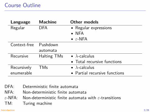
Course Outline
Language Machine Other modelsRegular DFA • Regular expressions
• NFA• 𝜀-NFA
Context-free Pushdownautomata
Recursive Halting TMs • 𝜆-calculus• Total recursive functions
Recursivelyenumerable
TMs • 𝜆-calculus• Partial recursive functions
DFA: Deterministic finite automataNFA: Non-deterministic finite automata𝜀-NFA: Non-deterministic finite automata with 𝜀-transitionsTM: Turing machine
Introduction 3/28
Computability (Decidability)
QuestionWhat can a computer do at all?
DefinitionA computable (or decidable) problem is a problem than can be solved by acomputer (informal definition).
Introduction 4/28
Computability (Decidability)
QuestionWhat can a computer do at all?
DefinitionA computable (or decidable) problem is a problem than can be solved by acomputer (informal definition).
Introduction 5/28

Computability (Decidability)
Example (The halting problem: An undecidable problem)Given an program P and an input I, to decide if the program will halt orwill run forever.
The halting algorithm
P Yes
I No
Introduction 6/28

Algorithmic Complexity (Tractability)
Comparison of several time complexity functions
𝑓(𝑛) 10 50 100log 𝑛 2.3 sec 3.9 sec 4.6 sec𝑛 10 sec 50 sec 1.7 min𝑛2 1.7 min 41.7 min 2.8 h2𝑛 17.1 min 358.001 c 4 × 10²⁰ c3𝑛 16.4 h 2.3 × 10¹⁴ c 1.6 × 1038 c𝑛! 42 d 9.7 × 1054 c 3 × 10148 c
Introduction 7/28
Algorithmic Complexity (Tractability)
QuestionWhat can a computer do efficiently?
DefinitionA tractable problem is a problem than can be solved by a computer algorithmthat run in polynomial time.
Introduction 8/28

Algorithmic Complexity (Tractability)
QuestionWhat can a computer do efficiently?
DefinitionA tractable problem is a problem than can be solved by a computer algorithmthat run in polynomial time.
Introduction 9/28

Algorithmic Complexity (Tractability)
DefinitionA literal is an atomic formula (propositional variable) or the negation of anatomic formula.
DefinitionA (propositional logic) formula 𝐹 is said to be in conjunctive normal form,if and only if,
𝐹 has the form 𝐹1 ∧ ⋯ ∧ 𝐹𝑛, 𝑛 ≥ 1,where each 𝐹1, … , 𝐹𝑛 is a disjunction of literals.
Introduction 10/28
Algorithmic Complexity (Tractability)
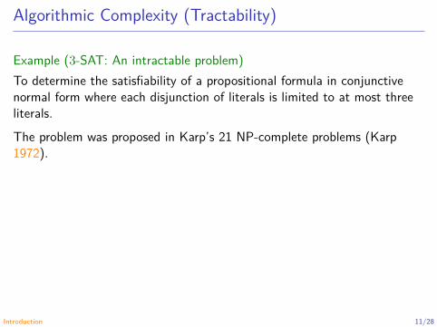
Example (3-SAT: An intractable problem)To determine the satisfiability of a propositional formula in conjunctivenormal form where each disjunction of literals is limited to at most threeliterals.The problem was proposed in Karp’s 21 NP-complete problems (Karp1972).
Introduction 11/28

Algorithmic Complexity (Tractability)
3-SAT better deterministic algorithmic complexity
𝑂(1.3303𝑛) Makino, Tamaki and Yamamoto (2011)𝑂(1.33334𝑛) Moser and Scheder (2011)𝑂(1.439𝑛) Kutzkov and Scheder (2010)𝑂(1.465𝑛) Scheder (2008)𝑂(1.473𝑛) Brueggemann and Kern (2004)𝑂(1.481𝑛) Dantsin, Goerdt, Hirsch, Kannan, Kleinberg, Papadimitriou,
Raghavan and Schöning (2002)𝑂(1.497𝑛) Schiermeyer (1996)𝑂(1.505𝑛) Kullmann (1999)𝑂(1.681𝑛) Monien and Speckenmeyer (1979, 1985)
Introduction 12/28
Algorithmic Complexity (Tractability)
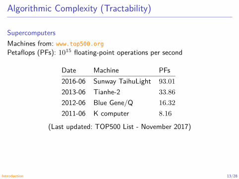
SupercomputersMachines from: www.top500.orgPetaflops (PFs): 1015 floating-point operations per second
Date Machine PFs2016-06 Sunway TaihuLight 93.012013-06 Tianhe-2 33.862012-06 Blue Gene/Q 16.322011-06 K computer 8.16
(Last updated: TOP500 List - November 2017)
Introduction 13/28
Algorithmic Complexity (Tractability)
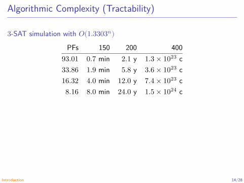
3-SAT simulation with 𝑂(1.3303𝑛)PFs 150 200 400
93.01 0.7 min 2.1 y 1.3 × 10²³ c33.86 1.9 min 5.8 y 3.6 × 10²³ c16.32 4.0 min 12.0 y 7.4 × 10²³ c8.16 8.0 min 24.0 y 1.5 × 1024 c
Introduction 14/28
Computability and Algorithmic Complexity
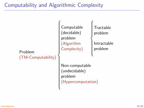
Problem(TM-Computability)
⎧{{{{{{{{{⎨{{{{{{{{{⎩
Computable(decidable)problem(AlgorithmComplexity)
⎧{{{{⎨{{{{⎩
Tractableproblem
Intractableproblem
Non-computable(undecidable)problem(Hypercomputation)
Introduction 15/28

Some Paradigms of Programming
Imperative: Describe computation in terms of state-transformingoperations such as assignment. Programming is done with statements.Logic: Predicate calculus as a programming language. Programming isdone with sentences.Functional: Describe computation in terms of (mathematical) functions.Programming is done with expressions.
Examples
Imperative⎧{⎨{⎩
CC++Java
Logic {CLP(R)Prolog
Functional
⎧{{{⎨{{{⎩
Standard MLErlang
Pure⎧{⎨{⎩
CleanHaskellIdris
Introduction 16/28

Pure Functional Programming
Side effects“A side effect introduces a dependency between the global state of thesystem and the behaviour of a function... Side effects are essentially invisibleinputs to, or outputs from, functions.” (O’Sullivan, Goerzen and Stewart2008, p. 27)
Introduction 17/28

Pure Functional Programming
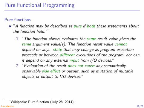
Pure functions“A function may be described as pure if both these statements aboutthe function hold:”†
1. “The function always evaluates the same result value given thesame argument value(s). The function result value cannotdepend on any... state that may change as program executionproceeds or between different executions of the program, nor canit depend on any external input from I/O devices.”
2. “Evaluation of the result does not cause any semanticallyobservable side effect or output, such as mutation of mutableobjects or output to I/O devices.”
†Wikipedia: Pure function (July 28, 2014).Introduction 18/28
Pure Functional Programming
Pure functions“A function may be described as pure if both these statements aboutthe function hold:”†
1. “The function always evaluates the same result value given thesame argument value(s). The function result value cannotdepend on any... state that may change as program executionproceeds or between different executions of the program, nor canit depend on any external input from I/O devices.”
2. “Evaluation of the result does not cause any semanticallyobservable side effect or output, such as mutation of mutableobjects or output to I/O devices.”
†Wikipedia: Pure function (July 28, 2014).Introduction 19/28
Pure Functional Programming
Pure functions“...take all their input as explicit arguments, and produce all theiroutput as explicit results.” (Hutton 2016, § 10.1)
Introduction 20/28

Pure Functional Programming
Referential transparencyEquals can be replaced by equals
“By definition, a function in Haskell defines a fixed relation betweeninputs and output: whenever a function 𝑓 is applied to the argumentvalue 𝑎𝑟𝑔 it will produce the same output no matter what the overallstate of the computation is. Haskell, like any other pure functionallanguage, is said to be ‘referentially transparent’ or ‘side-effect free’.This property does not hold for imperative languages...” (Grune, Bal,Jacobs and Langendoen 2003, pp. 544–545)
Introduction 21/28

Pure Functional Programming
Referential transparencyEquals can be replaced by equals“By definition, a function in Haskell defines a fixed relation betweeninputs and output: whenever a function 𝑓 is applied to the argumentvalue 𝑎𝑟𝑔 it will produce the same output no matter what the overallstate of the computation is. Haskell, like any other pure functionallanguage, is said to be ‘referentially transparent’ or ‘side-effect free’.This property does not hold for imperative languages...” (Grune, Bal,Jacobs and Langendoen 2003, pp. 544–545)
Introduction 22/28
Pure Functional Programming
Reasoning about (pure) functional programsEquational reasoning + induction + co-induction + …
Introduction 23/28

Reading
HomeworkTo read from the textbook the following sections:§ 1.1. Why Study Automata Theory?§ 1.2. Introduction to Formal Proofs§ 1.3. Additional Forms of Proofs
Introduction 24/28
References
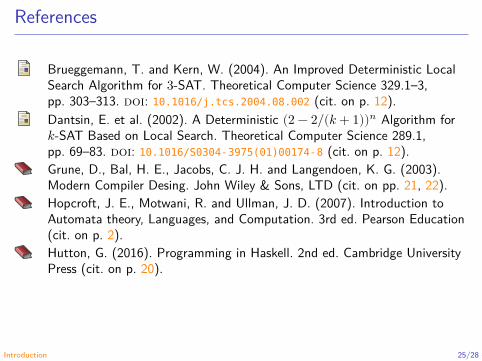
Brueggemann, T. and Kern, W. (2004). An Improved Deterministic LocalSearch Algorithm for 3-SAT. Theoretical Computer Science 329.1–3,pp. 303–313. doi: 10.1016/j.tcs.2004.08.002 (cit. on p. 12).Dantsin, E. et al. (2002). A Deterministic (2 − 2/(𝑘 + 1))𝑛 Algorithm for𝑘-SAT Based on Local Search. Theoretical Computer Science 289.1,pp. 69–83. doi: 10.1016/S0304-3975(01)00174-8 (cit. on p. 12).Grune, D., Bal, H. E., Jacobs, C. J. H. and Langendoen, K. G. (2003).Modern Compiler Desing. John Wiley & Sons, LTD (cit. on pp. 21, 22).Hopcroft, J. E., Motwani, R. and Ullman, J. D. (2007). Introduction toAutomata theory, Languages, and Computation. 3rd ed. Pearson Education(cit. on p. 2).Hutton, G. (2016). Programming in Haskell. 2nd ed. Cambridge UniversityPress (cit. on p. 20).
Introduction 25/28
References
Karp, R. M. (1972). Reducibility Among Combinatorial Problems. In:Complexity of Computer Computations. Ed. by Miller, R. E. andThatcher, J. W. Plenum Press, pp. 85–103. doi:10.1007/978-1-4684-2001-2_9 (cit. on p. 11).Kullmann, O. (1999). New Methods for 3-SAT Decision and Worst-CaseAnalysis. Theoretical Computer Science 223.1–2, pp. 1–72. doi:10.1016/S0304-3975(98)00017-6 (cit. on p. 12).Kutzkov, K. and Scheder, D. (2010). Using CSP to Improve Deterministic3-SAT. CoRR abs/1007.1166. url: https://arxiv.org/abs/1007.1166(cit. on p. 12).Makino, K., Tamaki, S. and Yamamoto, M. (2011). Derandomizing HSSWAlgorithm for 3-SAT. CoRR. url: https://arxiv.org/abs/1102.3766(cit. on p. 12).Monien, B. and Speckenmeyer, E. (1979). 3-Satisfiability is Testable in𝑂(1.62𝑟) Steps. Tech. rep. 3/1979. Reihe Theoretische Informatik,Universität-Gesamthochschule-Paderborn (cit. on p. 12).
Introduction 26/28

References
Monien, B. and Speckenmeyer, E. (1985). Solving Satisfiability in less than2𝑛 Steps. Discrete Applied Mathematics 10.3, pp. 287–295. doi:10.1016/0166-218X(85)90050-2 (cit. on p. 12).Moser, R. A. and Scheder, D. (2011). A Full Derandomization ofSchöning’s 𝑘-SAT Algorithm. In: Proceedings of the Forty-third AnnualACM Symposium on Theory of Computing (STOC 2011), pp. 245–252.doi: 10.1145/1993636.1993670 (cit. on p. 12).O’Sullivan, B., Goerzen, J. and Stewart, D. (2008). Real World Haskell.O’REILLY (cit. on p. 17).Scheder, D. (2008). Guided Search and a Faster Deterministic Algorithm for3-SAT. In: Proc. of the 8th Latin American Symposium on TheoreticalInformatic (LATIN 2008). Ed. by Laber, E. S., Bornstein, C.,Nogueira, T. L. and Faria, L. Vol. 4957. Lecture Notes in Computer Science.Springer, pp. 60–71. doi: 10.1007/978-3-540-78773-0_6 (cit. on p. 12).
Introduction 27/28
References
Schiermeyer, I. (1996). Pure Literal Look Ahead: An 𝑂(1.497𝑛)3-Satisfability Algorithm (Extended Abstract). Workshop on theSatisfability Problem, Siena 1996. url:http://gauss.ececs.uc.edu/franco_files/SAT96/sat-workshop-abstracts.html (cit. on p. 12).
Introduction 28/28
Automata and Formal Languages - CM0081Formal Proofs
Andrés Sicard-Ramírez
Universidad EAFIT
Semester 2018-1
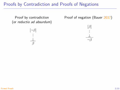
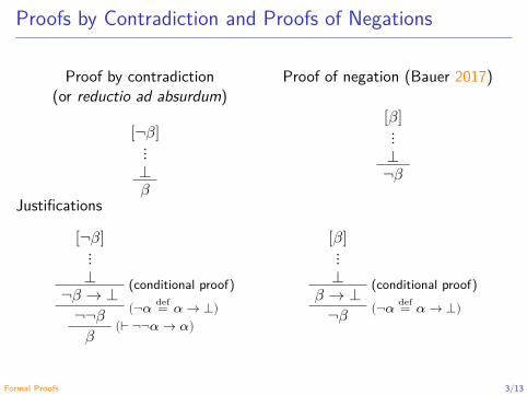
Proofs by Contradiction and Proofs of Negations
Proof by contradiction(or reductio ad absurdum)
[¬𝛽]⋮
⊥𝛽
Proof of negation (Bauer 2017)
[𝛽]⋮⊥¬𝛽
Justifications
[¬𝛽]⋮
⊥ (conditional proof)¬𝛽 → ⊥(¬𝛼 def= 𝛼 → ⊥)¬¬𝛽 (⊢ ¬¬𝛼 → 𝛼)𝛽
[𝛽]⋮
⊥ (conditional proof)𝛽 → ⊥(¬𝛼 def= 𝛼 → ⊥)¬𝛽
Formal Proofs 2/13
Proofs by Contradiction and Proofs of Negations
Proof by contradiction(or reductio ad absurdum)
[¬𝛽]⋮
⊥𝛽
Proof of negation (Bauer 2017)
[𝛽]⋮⊥¬𝛽
Justifications
[¬𝛽]⋮
⊥ (conditional proof)¬𝛽 → ⊥(¬𝛼 def= 𝛼 → ⊥)¬¬𝛽 (⊢ ¬¬𝛼 → 𝛼)𝛽
[𝛽]⋮
⊥ (conditional proof)𝛽 → ⊥(¬𝛼 def= 𝛼 → ⊥)¬𝛽
Formal Proofs 3/13

Inductive Proofs: Mathematical Induction
The induction principleLet 𝑆(𝑛) be a property about the natural numbers. If
we prove 𝑆(𝑖) (basis step) andwe prove that for all natural number 𝑛 ≥ 𝑖, 𝑆(𝑛) implies 𝑆(𝑛 + 1)(inductive step)
then we may conclude 𝑆(𝑛) for all 𝑛 ≥ 𝑖.
Formal Proofs 4/13
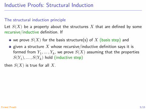
Inductive Proofs: Structural Induction
The structural induction principleLet 𝑆(𝑋) be a property about the structures 𝑋 that are defined by somerecursive/inductive definition. If
we prove 𝑆(𝑋) for the basis structure(s) of 𝑋 (basis step) andgiven a structure 𝑋 whose recursive/inductive definition says it isformed from 𝑌1, … , 𝑌𝑘, we prove 𝑆(𝑋) assuming that the properties𝑆(𝑌1), … , 𝑆(𝑌𝑘) hold (inductive step)
then 𝑆(𝑋) is true for all 𝑋.
Formal Proofs 5/13
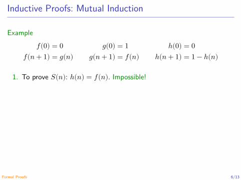
Inductive Proofs: Mutual Induction
Example𝑓(0) = 0 𝑔(0) = 1 ℎ(0) = 0
𝑓(𝑛 + 1) = 𝑔(𝑛) 𝑔(𝑛 + 1) = 𝑓(𝑛) ℎ(𝑛 + 1) = 1 − ℎ(𝑛)
1. To prove 𝑆(𝑛): ℎ(𝑛) = 𝑓(𝑛). Impossible!
2. To prove 𝑇 (𝑛): a) ℎ(𝑛) = 𝑓(𝑛) and b) ℎ(𝑛) = 1 − 𝑔(𝑛).
Formal Proofs 6/13
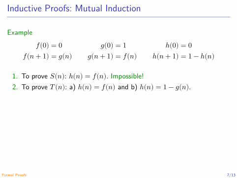
Inductive Proofs: Mutual Induction
Example𝑓(0) = 0 𝑔(0) = 1 ℎ(0) = 0
𝑓(𝑛 + 1) = 𝑔(𝑛) 𝑔(𝑛 + 1) = 𝑓(𝑛) ℎ(𝑛 + 1) = 1 − ℎ(𝑛)
1. To prove 𝑆(𝑛): ℎ(𝑛) = 𝑓(𝑛). Impossible!2. To prove 𝑇 (𝑛): a) ℎ(𝑛) = 𝑓(𝑛) and b) ℎ(𝑛) = 1 − 𝑔(𝑛).
Formal Proofs 7/13

Inductive Proofs: Mutual Induction
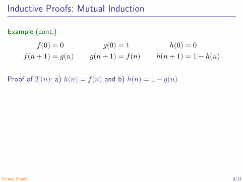
Example (cont.)
𝑓(0) = 0 𝑔(0) = 1 ℎ(0) = 0𝑓(𝑛 + 1) = 𝑔(𝑛) 𝑔(𝑛 + 1) = 𝑓(𝑛) ℎ(𝑛 + 1) = 1 − ℎ(𝑛)
Proof of 𝑇 (𝑛): a) ℎ(𝑛) = 𝑓(𝑛) and b) ℎ(𝑛) = 1 − 𝑔(𝑛).Basis step 𝑇 (0). Easy.Induction step 𝑇 (𝑛) ⇒ 𝑇 (𝑛 + 1):
a) ℎ(𝑛 + 1) = 1 − ℎ(𝑛) (def. of ℎ)= 𝑔(𝑛) (IH b)= 𝑓(𝑛 + 1) (def. of 𝑓)
b) ℎ(𝑛 + 1) = 1 − ℎ(𝑛) (def. of ℎ)= 1 − 𝑓(𝑛) (IH a)= 1 − 𝑔(𝑛 + 1) (def. of 𝑔)
Formal Proofs 8/13
Inductive Proofs: Mutual Induction
Example (cont.)
𝑓(0) = 0 𝑔(0) = 1 ℎ(0) = 0𝑓(𝑛 + 1) = 𝑔(𝑛) 𝑔(𝑛 + 1) = 𝑓(𝑛) ℎ(𝑛 + 1) = 1 − ℎ(𝑛)
Proof of 𝑇 (𝑛): a) ℎ(𝑛) = 𝑓(𝑛) and b) ℎ(𝑛) = 1 − 𝑔(𝑛).
Basis step 𝑇 (0). Easy.Induction step 𝑇 (𝑛) ⇒ 𝑇 (𝑛 + 1):
a) ℎ(𝑛 + 1) = 1 − ℎ(𝑛) (def. of ℎ)= 𝑔(𝑛) (IH b)= 𝑓(𝑛 + 1) (def. of 𝑓)
b) ℎ(𝑛 + 1) = 1 − ℎ(𝑛) (def. of ℎ)= 1 − 𝑓(𝑛) (IH a)= 1 − 𝑔(𝑛 + 1) (def. of 𝑔)
Formal Proofs 9/13

Inductive Proofs: Mutual Induction
Example (cont.)
𝑓(0) = 0 𝑔(0) = 1 ℎ(0) = 0𝑓(𝑛 + 1) = 𝑔(𝑛) 𝑔(𝑛 + 1) = 𝑓(𝑛) ℎ(𝑛 + 1) = 1 − ℎ(𝑛)
Proof of 𝑇 (𝑛): a) ℎ(𝑛) = 𝑓(𝑛) and b) ℎ(𝑛) = 1 − 𝑔(𝑛).Basis step 𝑇 (0). Easy.
Induction step 𝑇 (𝑛) ⇒ 𝑇 (𝑛 + 1):a) ℎ(𝑛 + 1) = 1 − ℎ(𝑛) (def. of ℎ)
= 𝑔(𝑛) (IH b)= 𝑓(𝑛 + 1) (def. of 𝑓)
b) ℎ(𝑛 + 1) = 1 − ℎ(𝑛) (def. of ℎ)= 1 − 𝑓(𝑛) (IH a)= 1 − 𝑔(𝑛 + 1) (def. of 𝑔)
Formal Proofs 10/13

Inductive Proofs: Mutual Induction
Example (cont.)
𝑓(0) = 0 𝑔(0) = 1 ℎ(0) = 0𝑓(𝑛 + 1) = 𝑔(𝑛) 𝑔(𝑛 + 1) = 𝑓(𝑛) ℎ(𝑛 + 1) = 1 − ℎ(𝑛)
Proof of 𝑇 (𝑛): a) ℎ(𝑛) = 𝑓(𝑛) and b) ℎ(𝑛) = 1 − 𝑔(𝑛).Basis step 𝑇 (0). Easy.Induction step 𝑇 (𝑛) ⇒ 𝑇 (𝑛 + 1):
a) ℎ(𝑛 + 1) = 1 − ℎ(𝑛) (def. of ℎ)= 𝑔(𝑛) (IH b)= 𝑓(𝑛 + 1) (def. of 𝑓)
b) ℎ(𝑛 + 1) = 1 − ℎ(𝑛) (def. of ℎ)= 1 − 𝑓(𝑛) (IH a)= 1 − 𝑔(𝑛 + 1) (def. of 𝑔)
Formal Proofs 11/13

Inductive Proofs: Mutual Induction
Example (cont.)
𝑓(0) = 0 𝑔(0) = 1 ℎ(0) = 0𝑓(𝑛 + 1) = 𝑔(𝑛) 𝑔(𝑛 + 1) = 𝑓(𝑛) ℎ(𝑛 + 1) = 1 − ℎ(𝑛)
Proof of 𝑇 (𝑛): a) ℎ(𝑛) = 𝑓(𝑛) and b) ℎ(𝑛) = 1 − 𝑔(𝑛).Basis step 𝑇 (0). Easy.Induction step 𝑇 (𝑛) ⇒ 𝑇 (𝑛 + 1):
a) ℎ(𝑛 + 1) = 1 − ℎ(𝑛) (def. of ℎ)= 𝑔(𝑛) (IH b)= 𝑓(𝑛 + 1) (def. of 𝑓)
b) ℎ(𝑛 + 1) = 1 − ℎ(𝑛) (def. of ℎ)= 1 − 𝑓(𝑛) (IH a)= 1 − 𝑔(𝑛 + 1) (def. of 𝑔)
Formal Proofs 12/13
References
Bauer, A. (2017). Five States of Accepting Constructive Mathematics. Bull.Amer. Math. Soc. 54.3, pp. 481–498. doi: 10.1090/bull/1556 (cit. onpp. 2, 3).
Formal Proofs 13/13
Automata and Formal Languages - CM0081The Central Concepts of Automata Theory
Andrés Sicard-Ramírez
Universidad EAFIT
Semester 2018-1

Alphabets and Words
DefinitionAn alphabet is a finite, non-empty set of symbols.
ExamplesΣ1 = {0, 1},Σ2 = {𝑎, 𝑏, … , 𝑧},Σ3 = {𝑥 ∣ 𝑥 is a Unicode codepoint }.
The Central Concepts of Automata Theory 2/34
Alphabets and Words
DefinitionAn alphabet is a finite, non-empty set of symbols.
ExamplesΣ1 = {0, 1},Σ2 = {𝑎, 𝑏, … , 𝑧},Σ3 = {𝑥 ∣ 𝑥 is a Unicode codepoint }.
The Central Concepts of Automata Theory 3/34

Alphabets and Words
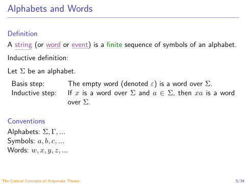
DefinitionA string (or word or event) is a finite sequence of symbols of an alphabet.Inductive definition:Let Σ be an alphabet.Basis step: The empty word (denoted 𝜀) is a word over Σ.Inductive step: If 𝑥 is a word over Σ and 𝑎 ∈ Σ, then 𝑥𝑎 is a word
over Σ.
ConventionsAlphabets: Σ, Γ, …Symbols: 𝑎, 𝑏, 𝑐, …Words: 𝑤, 𝑥, 𝑦, 𝑧, …
The Central Concepts of Automata Theory 4/34
Alphabets and Words
DefinitionA string (or word or event) is a finite sequence of symbols of an alphabet.Inductive definition:Let Σ be an alphabet.Basis step: The empty word (denoted 𝜀) is a word over Σ.Inductive step: If 𝑥 is a word over Σ and 𝑎 ∈ Σ, then 𝑥𝑎 is a word
over Σ.
ConventionsAlphabets: Σ, Γ, …Symbols: 𝑎, 𝑏, 𝑐, …Words: 𝑤, 𝑥, 𝑦, 𝑧, …
The Central Concepts of Automata Theory 5/34
Operations on Words
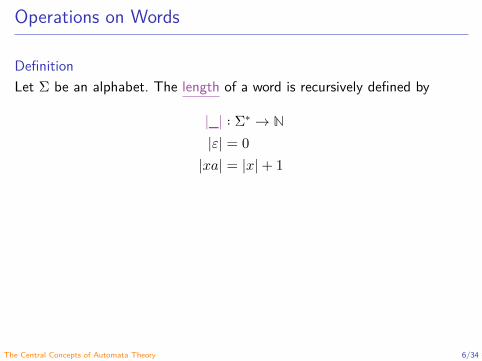
DefinitionLet Σ be an alphabet. The length of a word is recursively defined by
|_| ∶ Σ∗ → ℕ|𝜀| = 0
|𝑥𝑎| = |𝑥| + 1
The Central Concepts of Automata Theory 6/34

Operations on Words
DefinitionLet Σ be an alphabet. The concatenation of words is recursively defined by
_ · _ ∶ Σ∗ × Σ∗ → Σ∗
𝑥 · 𝜀 = 𝑥𝑥 · 𝑦𝑎 = (𝑥 · 𝑦)𝑎
Note: 𝑥 · 𝜀 = 𝜀 · 𝑥 = 𝑥 (that implies an algebraic structure)
NotationWe remove the dot in the concatenation.
The Central Concepts of Automata Theory 7/34

Operations on Words
DefinitionLet Σ be an alphabet. The concatenation of words is recursively defined by
_ · _ ∶ Σ∗ × Σ∗ → Σ∗
𝑥 · 𝜀 = 𝑥𝑥 · 𝑦𝑎 = (𝑥 · 𝑦)𝑎
Note: 𝑥 · 𝜀 = 𝜀 · 𝑥 = 𝑥 (that implies an algebraic structure)
NotationWe remove the dot in the concatenation.
The Central Concepts of Automata Theory 8/34

Operations on Words
DefinitionLet Σ be an alphabet. The concatenation of words is recursively defined by
_ · _ ∶ Σ∗ × Σ∗ → Σ∗
𝑥 · 𝜀 = 𝑥𝑥 · 𝑦𝑎 = (𝑥 · 𝑦)𝑎
Note: 𝑥 · 𝜀 = 𝜀 · 𝑥 = 𝑥 (that implies an algebraic structure)
NotationWe remove the dot in the concatenation.
The Central Concepts of Automata Theory 9/34

Operations on Words
ExampleLet Σ be an alphabet and let 𝑥 and 𝑦 be words over Σ. Prove that|𝑥𝑦| = |𝑥| + |𝑦|.
The Central Concepts of Automata Theory 10/34

Operations on Words
Proof.By structural induction on 𝑦.
(or by mathematical induction on |𝑦|).
Basis step (𝑦 = 𝜀):
(or |𝑦| = 0, then 𝑦 = 𝜀):
|𝑥𝜀| = |𝑥| (def. of concatenation)= |𝑥| + |𝜀| (def. of length)
Induction step (𝑦 = 𝑤𝑎):
(or |𝑦| = 𝑛 + 1, then 𝑦 = 𝑤𝑎 where|𝑤| = 𝑛):
|𝑥(𝑤𝑎)| = |𝑥𝑤(𝑎)| (def. of concatenation)= |𝑥𝑤| + 1 (def. of length)= |𝑥| + |𝑤| + 1 (IH)= |𝑥| + |𝑤𝑎| (def. of length)
The Central Concepts of Automata Theory 11/34

Operations on Words
Proof.By structural induction on 𝑦 (or by mathematical induction on |𝑦|).
Basis step (𝑦 = 𝜀) (or |𝑦| = 0, then 𝑦 = 𝜀):
|𝑥𝜀| = |𝑥| (def. of concatenation)= |𝑥| + |𝜀| (def. of length)
Induction step (𝑦 = 𝑤𝑎) (or |𝑦| = 𝑛 + 1, then 𝑦 = 𝑤𝑎 where |𝑤| = 𝑛):
|𝑥(𝑤𝑎)| = |𝑥𝑤(𝑎)| (def. of concatenation)= |𝑥𝑤| + 1 (def. of length)= |𝑥| + |𝑤| + 1 (IH)= |𝑥| + |𝑤𝑎| (def. of length)
The Central Concepts of Automata Theory 12/34
Operations on Words
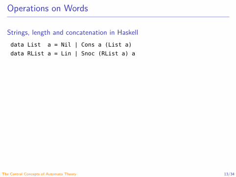
Strings, length and concatenation in Haskelldata List a = Nil | Cons a (List a)data RList a = Lin | Snoc (RList a) a
length' :: RList a -> Intlength' Lin = 0 -- Eq. 1length' (Snoc xs x) = 1 + length' xs -- Eq. 2
(+++) :: RList a -> RList a -> RList a(+++) xs Lin = xs -- Eq. 1(+++) xs (Snoc ys y) = Snoc (xs +++ ys) y -- Eq. 2
The Central Concepts of Automata Theory 13/34

Operations on Words
Strings, length and concatenation in Haskelldata List a = Nil | Cons a (List a)data RList a = Lin | Snoc (RList a) a
length' :: RList a -> Intlength' Lin = 0 -- Eq. 1length' (Snoc xs x) = 1 + length' xs -- Eq. 2
(+++) :: RList a -> RList a -> RList a(+++) xs Lin = xs -- Eq. 1(+++) xs (Snoc ys y) = Snoc (xs +++ ys) y -- Eq. 2
The Central Concepts of Automata Theory 14/34

Operations on Words
Strings, length and concatenation in Haskelldata List a = Nil | Cons a (List a)data RList a = Lin | Snoc (RList a) a
length' :: RList a -> Intlength' Lin = 0 -- Eq. 1length' (Snoc xs x) = 1 + length' xs -- Eq. 2
(+++) :: RList a -> RList a -> RList a(+++) xs Lin = xs -- Eq. 1(+++) xs (Snoc ys y) = Snoc (xs +++ ys) y -- Eq. 2
The Central Concepts of Automata Theory 15/34

Operations on Words
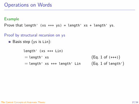
ExampleProve that length' (xs +++ ys) = length' xs + length' ys.
Proof by structural recursion on ys
Basis step (ys is Lin):
length' (xs +++ Lin)
= length' xs (Eq. 1 of (+++))= length' xs +++ length' Lin (Eq. 1 of length')
The Central Concepts of Automata Theory 16/34
Operations on Words
ExampleProve that length' (xs +++ ys) = length' xs + length' ys.
Proof by structural recursion on ys
Basis step (ys is Lin):
length' (xs +++ Lin)
= length' xs (Eq. 1 of (+++))= length' xs +++ length' Lin (Eq. 1 of length')
The Central Concepts of Automata Theory 17/34

Operations on Words
Induction step (ys is Snoc ys' y'):
length' (xs +++ (Snoc ys' y'))
= length' (Snoc (xs +++ ys') y')) (Eq. 2 of (+++))= 1 + length' (xs +++ ys') (Eq. 2 of length')= 1 + (length' xs + length' ys') (IH)= length' xs + (1 + length' ys') (arithmetic)= length' xs + length' (Snoc ys' y) (Eq. 2 of length')
The Central Concepts of Automata Theory 18/34

Operations on Words and Alphabets
DefinitionLet Σ be an alphabet. The power of words is recursively defined by
__ ∶ Σ∗ × ℕ → Σ∗
𝑥0 = 𝜀𝑥𝑛+1 = 𝑥𝑛𝑥
The Central Concepts of Automata Theory 19/34
Operations on Words and Alphabets
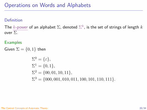
DefinitionThe 𝑘-power of an alphabet Σ, denoted Σ𝑘, is the set of strings of length 𝑘over Σ.
ExamplesGiven Σ = {0, 1} then
Σ0 = {𝜀},Σ1 = {0, 1},Σ2 = {00, 01, 10, 11},Σ3 = {000, 001, 010, 011, 100, 101, 110, 111}.
The Central Concepts of Automata Theory 20/34

Universal Language
DefinitionLet Σ be an alphabet. The universal language over Σ, denoted by Σ∗, is theset of all the strings over Σ.
The Central Concepts of Automata Theory 21/34
Languages
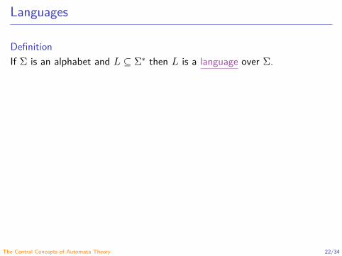
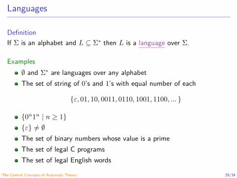
DefinitionIf Σ is an alphabet and 𝐿 ⊆ Σ∗ then 𝐿 is a language over Σ.
Examples∅ and Σ∗ are languages over any alphabetThe set of string of 0’s and 1’s with equal number of each
{𝜀, 01, 10, 0011, 0110, 1001, 1100, … }
{0𝑛1𝑛 ∣ 𝑛 ≥ 1}{𝜀} ≠ ∅The set of binary numbers whose value is a primeThe set of legal C programsThe set of legal English words
The Central Concepts of Automata Theory 22/34
Languages
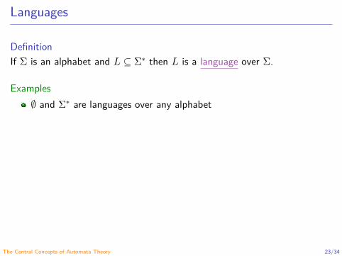
DefinitionIf Σ is an alphabet and 𝐿 ⊆ Σ∗ then 𝐿 is a language over Σ.
Examples∅ and Σ∗ are languages over any alphabet
The set of string of 0’s and 1’s with equal number of each
{𝜀, 01, 10, 0011, 0110, 1001, 1100, … }
{0𝑛1𝑛 ∣ 𝑛 ≥ 1}{𝜀} ≠ ∅The set of binary numbers whose value is a primeThe set of legal C programsThe set of legal English words
The Central Concepts of Automata Theory 23/34

Languages
DefinitionIf Σ is an alphabet and 𝐿 ⊆ Σ∗ then 𝐿 is a language over Σ.
Examples∅ and Σ∗ are languages over any alphabetThe set of string of 0’s and 1’s with equal number of each
{𝜀, 01, 10, 0011, 0110, 1001, 1100, … }
{0𝑛1𝑛 ∣ 𝑛 ≥ 1}{𝜀} ≠ ∅The set of binary numbers whose value is a primeThe set of legal C programsThe set of legal English words
The Central Concepts of Automata Theory 24/34

Languages
DefinitionIf Σ is an alphabet and 𝐿 ⊆ Σ∗ then 𝐿 is a language over Σ.
Examples∅ and Σ∗ are languages over any alphabetThe set of string of 0’s and 1’s with equal number of each
{𝜀, 01, 10, 0011, 0110, 1001, 1100, … }
{0𝑛1𝑛 ∣ 𝑛 ≥ 1}
{𝜀} ≠ ∅The set of binary numbers whose value is a primeThe set of legal C programsThe set of legal English words
The Central Concepts of Automata Theory 25/34

Languages
DefinitionIf Σ is an alphabet and 𝐿 ⊆ Σ∗ then 𝐿 is a language over Σ.
Examples∅ and Σ∗ are languages over any alphabetThe set of string of 0’s and 1’s with equal number of each
{𝜀, 01, 10, 0011, 0110, 1001, 1100, … }
{0𝑛1𝑛 ∣ 𝑛 ≥ 1}{𝜀} ≠ ∅
The set of binary numbers whose value is a primeThe set of legal C programsThe set of legal English words
The Central Concepts of Automata Theory 26/34

Languages
DefinitionIf Σ is an alphabet and 𝐿 ⊆ Σ∗ then 𝐿 is a language over Σ.
Examples∅ and Σ∗ are languages over any alphabetThe set of string of 0’s and 1’s with equal number of each
{𝜀, 01, 10, 0011, 0110, 1001, 1100, … }
{0𝑛1𝑛 ∣ 𝑛 ≥ 1}{𝜀} ≠ ∅The set of binary numbers whose value is a prime
The set of legal C programsThe set of legal English words
The Central Concepts of Automata Theory 27/34
Languages
DefinitionIf Σ is an alphabet and 𝐿 ⊆ Σ∗ then 𝐿 is a language over Σ.
Examples∅ and Σ∗ are languages over any alphabetThe set of string of 0’s and 1’s with equal number of each
{𝜀, 01, 10, 0011, 0110, 1001, 1100, … }
{0𝑛1𝑛 ∣ 𝑛 ≥ 1}{𝜀} ≠ ∅The set of binary numbers whose value is a primeThe set of legal C programs
The set of legal English words
The Central Concepts of Automata Theory 28/34
Languages
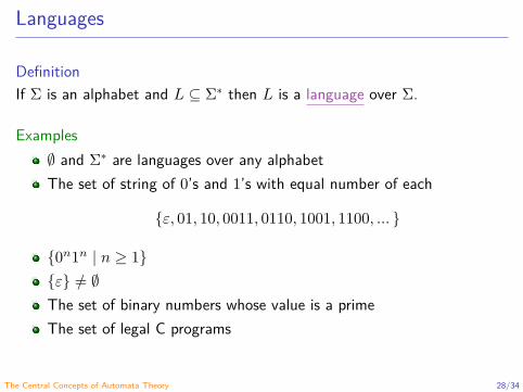
DefinitionIf Σ is an alphabet and 𝐿 ⊆ Σ∗ then 𝐿 is a language over Σ.
Examples∅ and Σ∗ are languages over any alphabetThe set of string of 0’s and 1’s with equal number of each
{𝜀, 01, 10, 0011, 0110, 1001, 1100, … }
{0𝑛1𝑛 ∣ 𝑛 ≥ 1}{𝜀} ≠ ∅The set of binary numbers whose value is a primeThe set of legal C programsThe set of legal English words
The Central Concepts of Automata Theory 29/34

Problems
DefinitionLet 𝐿 ⊆ Σ∗ be a language and let 𝑤 ∈ Σ∗ be word. To decide whether ornot 𝑤 ∈ 𝐿 is the decision problem on the language 𝐿.
Problem = decision problem?It is a language or a problem?Is the problem decidable or undecidable?Is the problem tractable or intractable?
The Central Concepts of Automata Theory 30/34
Problems
DefinitionLet 𝐿 ⊆ Σ∗ be a language and let 𝑤 ∈ Σ∗ be word. To decide whether ornot 𝑤 ∈ 𝐿 is the decision problem on the language 𝐿.
Problem = decision problem?
It is a language or a problem?Is the problem decidable or undecidable?Is the problem tractable or intractable?
The Central Concepts of Automata Theory 31/34

Problems
DefinitionLet 𝐿 ⊆ Σ∗ be a language and let 𝑤 ∈ Σ∗ be word. To decide whether ornot 𝑤 ∈ 𝐿 is the decision problem on the language 𝐿.
Problem = decision problem?It is a language or a problem?
Is the problem decidable or undecidable?Is the problem tractable or intractable?
The Central Concepts of Automata Theory 32/34

Problems
DefinitionLet 𝐿 ⊆ Σ∗ be a language and let 𝑤 ∈ Σ∗ be word. To decide whether ornot 𝑤 ∈ 𝐿 is the decision problem on the language 𝐿.
Problem = decision problem?It is a language or a problem?Is the problem decidable or undecidable?
Is the problem tractable or intractable?
The Central Concepts of Automata Theory 33/34
Problems
DefinitionLet 𝐿 ⊆ Σ∗ be a language and let 𝑤 ∈ Σ∗ be word. To decide whether ornot 𝑤 ∈ 𝐿 is the decision problem on the language 𝐿.
Problem = decision problem?It is a language or a problem?Is the problem decidable or undecidable?Is the problem tractable or intractable?
The Central Concepts of Automata Theory 34/34
Automata and Formal Languages - CM0081Determinist Finite Automata
Andrés Sicard-Ramírez
Universidad EAFIT
Semester 2018-1

Formal Languages: Origins
Source areas (Greibach 1981, p. 14)Logic and recursive-function theorySwitching circuit theory and logic designModelling of biological systems (brain activity)Mathematical and computation linguisticsComputer programming and the design of Algol and otherproblem-oriented languages
Determinist Finite Automata 2/32
Finite Automata
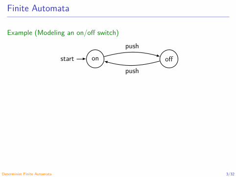
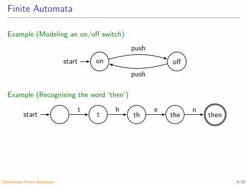
Example (Modeling an on/off switch)
onstart off
push
push
Example (Recognising the word ‘then’)
start t th the thent h e n
Determinist Finite Automata 3/32
Finite Automata
Example (Modeling an on/off switch)
onstart off
push
push
Example (Recognising the word ‘then’)
start t th the thent h e n
Determinist Finite Automata 4/32

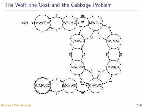
The Wolf, the Goat and the Cabbage Problem“A man with a wolf, goat, and cabbage is onthe left bank of a river. There is a boat largeenough to carry the man and only one of theother three. The man and his entouragewish to cross to the right bank, and the mancan ferry each across, one at a time.However, if the man leaves the wolf andgoat unattended on either shore, the wolfwill surely eat the goat. Similarly, if the goatand cabbage are left unattended, the goatwill eat the cabbage. Is it possible to crossthe river without the goat or cabbage beingeaten?” (Hopcroft and Ullman 1979, p. 14)†
†The illustration is from the cover of (Levitin 2006).Determinist Finite Automata 5/32
The Wolf, the Goat and the Cabbage Problem
MWGC/∅start WC/MG MWC/G
C/MWG W/MGC
MGC/W MWG/C
G/MWCMG/WC∅/MWGC
g
g
mm
w
g
c w
g
c
c
g
wc
g
w
g
g
m
m
Determinist Finite Automata 6/32
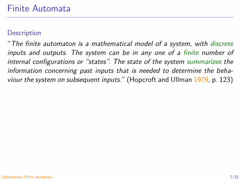
Finite Automata
Description“The finite automaton is a mathematical model of a system, with discreteinputs and outputs. The system can be in any one of a finite number ofinternal configurations or “states”. The state of the system summarizes theinformation concerning past inputs that is needed to determine the beha-viour the system on subsequent inputs.” (Hopcroft and Ullman 1979, p. 123)
Determinist Finite Automata 7/32
Deterministic Finite Automata
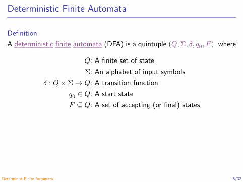
DefinitionA deterministic finite automata (DFA) is a quintuple (𝑄, Σ, 𝛿, 𝑞0, 𝐹 ), where
𝑄: A finite set of stateΣ: An alphabet of input symbols
𝛿 ∶ 𝑄 × Σ → 𝑄: A transition function𝑞0 ∈ 𝑄: A start state𝐹 ⊆ 𝑄: A set of accepting (or final) states
Determinist Finite Automata 8/32
DFA Representations
Transition diagramTransition tableDetailed description
Determinist Finite Automata 9/32

Transition Diagram
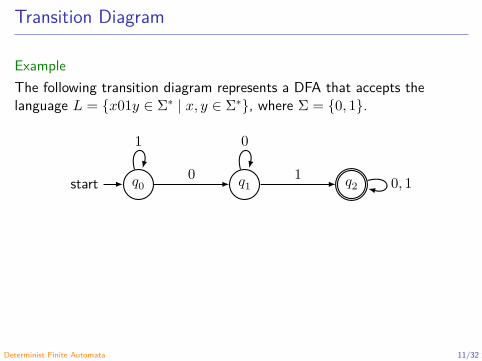
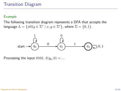
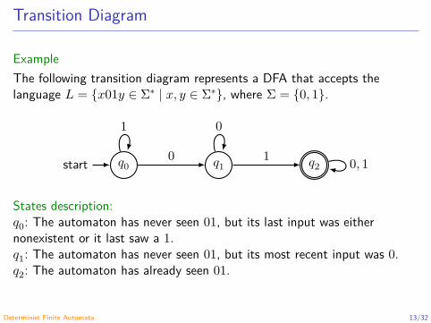
ExampleThe following transition diagram represents a DFA that accepts thelanguage 𝐿 = {𝑥01𝑦 ∈ Σ∗ ∣ 𝑥, 𝑦 ∈ Σ∗}, where Σ = {0, 1}.
𝑞0start 𝑞1 𝑞20
1
1
0
0, 1
States description:𝑞0: The automaton has never seen 01, but its last input was eithernonexistent or it last saw a 1.𝑞1: The automaton has never seen 01, but its most recent input was 0.𝑞2: The automaton has already seen 01.
Determinist Finite Automata 10/32
Transition Diagram
ExampleThe following transition diagram represents a DFA that accepts thelanguage 𝐿 = {𝑥01𝑦 ∈ Σ∗ ∣ 𝑥, 𝑦 ∈ Σ∗}, where Σ = {0, 1}.
𝑞0start 𝑞1 𝑞20
1
1
0
0, 1
States description:𝑞0: The automaton has never seen 01, but its last input was eithernonexistent or it last saw a 1.𝑞1: The automaton has never seen 01, but its most recent input was 0.𝑞2: The automaton has already seen 01.
Determinist Finite Automata 11/32
Transition Diagram
ExampleThe following transition diagram represents a DFA that accepts thelanguage 𝐿 = {𝑥01𝑦 ∈ Σ∗ ∣ 𝑥, 𝑦 ∈ Σ∗}, where Σ = {0, 1}.
𝑞0start 𝑞1 𝑞20
1
1
0
0, 1
Processing the input 0101: 𝛿(𝑞0, 0) = …
States description:𝑞0: The automaton has never seen 01, but its last input was eithernonexistent or it last saw a 1.𝑞1: The automaton has never seen 01, but its most recent input was 0.𝑞2: The automaton has already seen 01.
Determinist Finite Automata 12/32
Transition Diagram
ExampleThe following transition diagram represents a DFA that accepts thelanguage 𝐿 = {𝑥01𝑦 ∈ Σ∗ ∣ 𝑥, 𝑦 ∈ Σ∗}, where Σ = {0, 1}.
𝑞0start 𝑞1 𝑞20
1
1
0
0, 1
States description:𝑞0: The automaton has never seen 01, but its last input was eithernonexistent or it last saw a 1.𝑞1: The automaton has never seen 01, but its most recent input was 0.𝑞2: The automaton has already seen 01.
Determinist Finite Automata 13/32

Transition Tables and Detailed Descriptions
Example
𝑞0start 𝑞1 𝑞20
1
1
0
0, 1
Transition table:0 1
→ 𝑞0 𝑞1 𝑞0𝑞1 𝑞1 𝑞2
∗𝑞2 𝑞2 𝑞2
Detailed descriptions:𝑄 = {𝑞0, 𝑞1, 𝑞2}, Σ = {0, 1}, 𝑞0 (start state),{𝑞2} (set of accepting states) and 𝛿 ∶ 𝑄 × Σ → 𝑄where
𝛿(𝑞0, 0) = 𝑞1, 𝛿(𝑞0, 1) = 𝑞0,𝛿(𝑞1, 0) = 𝑞1, 𝛿(𝑞1, 1) = 𝑞2,𝛿(𝑞2, 0) = 𝑞2, 𝛿(𝑞2, 1) = 𝑞2.
Determinist Finite Automata 14/32

Transition Tables and Detailed Descriptions
Example
𝑞0start 𝑞1 𝑞20
1
1
0
0, 1
Transition table:0 1
→ 𝑞0 𝑞1 𝑞0𝑞1 𝑞1 𝑞2
∗𝑞2 𝑞2 𝑞2
Detailed descriptions:𝑄 = {𝑞0, 𝑞1, 𝑞2}, Σ = {0, 1}, 𝑞0 (start state),{𝑞2} (set of accepting states) and 𝛿 ∶ 𝑄 × Σ → 𝑄where
𝛿(𝑞0, 0) = 𝑞1, 𝛿(𝑞0, 1) = 𝑞0,𝛿(𝑞1, 0) = 𝑞1, 𝛿(𝑞1, 1) = 𝑞2,𝛿(𝑞2, 0) = 𝑞2, 𝛿(𝑞2, 1) = 𝑞2.
Determinist Finite Automata 15/32
Extension of the Transition Function for DFAs
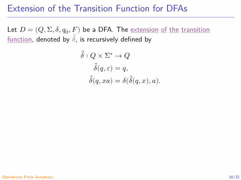
Let 𝐷 = (𝑄, Σ, 𝛿, 𝑞0, 𝐹 ) be a DFA. The extension of the transitionfunction, denoted by 𝛿, is recursively defined by
𝛿 ∶ 𝑄 × Σ∗ → 𝑄𝛿(𝑞, 𝜀) = 𝑞,
𝛿(𝑞, 𝑥𝑎) = 𝛿( 𝛿(𝑞, 𝑥), 𝑎).
Determinist Finite Automata 16/32

Extension of the Transition Function for DFAs
Example
𝑞0start 𝑞1 𝑞20
1
1
0
0, 1
𝛿(𝑞0, 0101) = 𝛿( 𝛿(𝑞0, 010), 1)= 𝛿(𝛿( 𝛿(𝑞0, 01), 0), 1)= 𝛿(𝛿(𝛿( 𝛿(𝑞0, 0), 1), 0), 1)= 𝛿(𝛿(𝛿(𝛿( 𝛿(𝑞0, 𝜀), 0), 1), 0), 1)= 𝛿(𝛿(𝛿(𝛿(𝑞0, 0), 1), 0), 1)= 𝛿(𝛿(𝛿(𝑞1, 1), 0), 1)= 𝛿(𝛿(𝑞2, 0), 1)= 𝛿(𝑞2, 1) = 𝑞2
Determinist Finite Automata 17/32

Extension of the Transition Function for DFAs
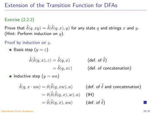
Exercise (2.2.2)
Prove that 𝛿(𝑞, 𝑥𝑦) = 𝛿( 𝛿(𝑞, 𝑥), 𝑦) for any state 𝑞 and strings 𝑥 and 𝑦.(Hint: Perform induction on 𝑦).
Proof by induction on 𝑦.Basis step (𝑦 = 𝜀)
𝛿( 𝛿(𝑞, 𝑥), 𝜀) = 𝛿(𝑞, 𝑥) (def. of 𝛿)= 𝛿(𝑞, 𝑥𝜀) (def. of concatenation)
Inductive step (𝑦 = 𝑤𝑎)
𝛿(𝑞, 𝑥 · 𝑤𝑎) = 𝛿( 𝛿(𝑞, 𝑥𝑤), 𝑎) (def. of 𝛿 and concatenation)= 𝛿( 𝛿( 𝛿(𝑞, 𝑥), 𝑤), 𝑎) (IH)= 𝛿( 𝛿(𝑞, 𝑥), 𝑤𝑎) (def. of 𝛿)
Determinist Finite Automata 18/32

Extension of the Transition Function for DFAs
Exercise (2.2.2)
Prove that 𝛿(𝑞, 𝑥𝑦) = 𝛿( 𝛿(𝑞, 𝑥), 𝑦) for any state 𝑞 and strings 𝑥 and 𝑦.(Hint: Perform induction on 𝑦).
Proof by induction on 𝑦.Basis step (𝑦 = 𝜀)
𝛿( 𝛿(𝑞, 𝑥), 𝜀) = 𝛿(𝑞, 𝑥) (def. of 𝛿)= 𝛿(𝑞, 𝑥𝜀) (def. of concatenation)
Inductive step (𝑦 = 𝑤𝑎)
𝛿(𝑞, 𝑥 · 𝑤𝑎) = 𝛿( 𝛿(𝑞, 𝑥𝑤), 𝑎) (def. of 𝛿 and concatenation)= 𝛿( 𝛿( 𝛿(𝑞, 𝑥), 𝑤), 𝑎) (IH)= 𝛿( 𝛿(𝑞, 𝑥), 𝑤𝑎) (def. of 𝛿)
Determinist Finite Automata 19/32
Extension of the Transition Function for DFAs
Exercise (2.2.2)
Prove that 𝛿(𝑞, 𝑥𝑦) = 𝛿( 𝛿(𝑞, 𝑥), 𝑦) for any state 𝑞 and strings 𝑥 and 𝑦.(Hint: Perform induction on 𝑦).
Proof by induction on 𝑦.Basis step (𝑦 = 𝜀)
𝛿( 𝛿(𝑞, 𝑥), 𝜀) = 𝛿(𝑞, 𝑥) (def. of 𝛿)= 𝛿(𝑞, 𝑥𝜀) (def. of concatenation)
Inductive step (𝑦 = 𝑤𝑎)
𝛿(𝑞, 𝑥 · 𝑤𝑎) = 𝛿( 𝛿(𝑞, 𝑥𝑤), 𝑎) (def. of 𝛿 and concatenation)= 𝛿( 𝛿( 𝛿(𝑞, 𝑥), 𝑤), 𝑎) (IH)= 𝛿( 𝛿(𝑞, 𝑥), 𝑤𝑎) (def. of 𝛿)
Determinist Finite Automata 20/32

Extension of the Transition Function for DFAs
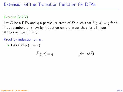
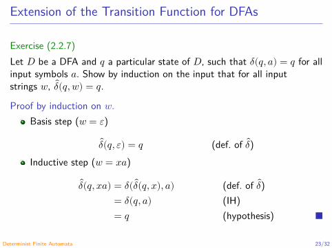
Exercise (2.2.7)Let 𝐷 be a DFA and 𝑞 a particular state of 𝐷, such that 𝛿(𝑞, 𝑎) = 𝑞 for allinput symbols 𝑎. Show by induction on the input that for all inputstrings 𝑤, 𝛿(𝑞, 𝑤) = 𝑞.
Proof by induction on 𝑤.Basis step (𝑤 = 𝜀)
𝛿(𝑞, 𝜀) = 𝑞 (def. of 𝛿)Inductive step (𝑤 = 𝑥𝑎)
𝛿(𝑞, 𝑥𝑎) = 𝛿( 𝛿(𝑞, 𝑥), 𝑎) (def. of 𝛿)= 𝛿(𝑞, 𝑎) (IH)= 𝑞 (hypothesis)
Determinist Finite Automata 21/32
Extension of the Transition Function for DFAs
Exercise (2.2.7)Let 𝐷 be a DFA and 𝑞 a particular state of 𝐷, such that 𝛿(𝑞, 𝑎) = 𝑞 for allinput symbols 𝑎. Show by induction on the input that for all inputstrings 𝑤, 𝛿(𝑞, 𝑤) = 𝑞.
Proof by induction on 𝑤.Basis step (𝑤 = 𝜀)
𝛿(𝑞, 𝜀) = 𝑞 (def. of 𝛿)
Inductive step (𝑤 = 𝑥𝑎)
𝛿(𝑞, 𝑥𝑎) = 𝛿( 𝛿(𝑞, 𝑥), 𝑎) (def. of 𝛿)= 𝛿(𝑞, 𝑎) (IH)= 𝑞 (hypothesis)
Determinist Finite Automata 22/32
Extension of the Transition Function for DFAs
Exercise (2.2.7)Let 𝐷 be a DFA and 𝑞 a particular state of 𝐷, such that 𝛿(𝑞, 𝑎) = 𝑞 for allinput symbols 𝑎. Show by induction on the input that for all inputstrings 𝑤, 𝛿(𝑞, 𝑤) = 𝑞.
Proof by induction on 𝑤.Basis step (𝑤 = 𝜀)
𝛿(𝑞, 𝜀) = 𝑞 (def. of 𝛿)Inductive step (𝑤 = 𝑥𝑎)
𝛿(𝑞, 𝑥𝑎) = 𝛿( 𝛿(𝑞, 𝑥), 𝑎) (def. of 𝛿)= 𝛿(𝑞, 𝑎) (IH)= 𝑞 (hypothesis)
Determinist Finite Automata 23/32

Regular Languages
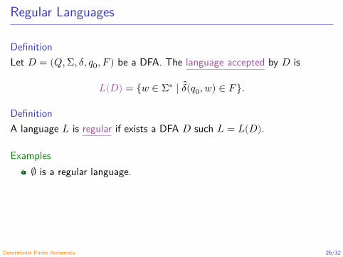
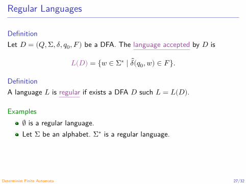
DefinitionLet 𝐷 = (𝑄, Σ, 𝛿, 𝑞0, 𝐹 ) be a DFA. The language accepted by 𝐷 is
𝐿(𝐷) = {𝑤 ∈ Σ∗ ∣ 𝛿(𝑞0, 𝑤) ∈ 𝐹}.
DefinitionA language 𝐿 is regular if exists a DFA 𝐷 such 𝐿 = 𝐿(𝐷).
Examples∅ is a regular language.Let Σ be an alphabet. Σ∗ is a regular language.
Determinist Finite Automata 24/32

Regular Languages
DefinitionLet 𝐷 = (𝑄, Σ, 𝛿, 𝑞0, 𝐹 ) be a DFA. The language accepted by 𝐷 is
𝐿(𝐷) = {𝑤 ∈ Σ∗ ∣ 𝛿(𝑞0, 𝑤) ∈ 𝐹}.
DefinitionA language 𝐿 is regular if exists a DFA 𝐷 such 𝐿 = 𝐿(𝐷).
Examples∅ is a regular language.Let Σ be an alphabet. Σ∗ is a regular language.
Determinist Finite Automata 25/32
Regular Languages
DefinitionLet 𝐷 = (𝑄, Σ, 𝛿, 𝑞0, 𝐹 ) be a DFA. The language accepted by 𝐷 is
𝐿(𝐷) = {𝑤 ∈ Σ∗ ∣ 𝛿(𝑞0, 𝑤) ∈ 𝐹}.
DefinitionA language 𝐿 is regular if exists a DFA 𝐷 such 𝐿 = 𝐿(𝐷).
Examples∅ is a regular language.
Let Σ be an alphabet. Σ∗ is a regular language.
Determinist Finite Automata 26/32
Regular Languages
DefinitionLet 𝐷 = (𝑄, Σ, 𝛿, 𝑞0, 𝐹 ) be a DFA. The language accepted by 𝐷 is
𝐿(𝐷) = {𝑤 ∈ Σ∗ ∣ 𝛿(𝑞0, 𝑤) ∈ 𝐹}.
DefinitionA language 𝐿 is regular if exists a DFA 𝐷 such 𝐿 = 𝐿(𝐷).
Examples∅ is a regular language.Let Σ be an alphabet. Σ∗ is a regular language.
Determinist Finite Automata 27/32
Regular Languages
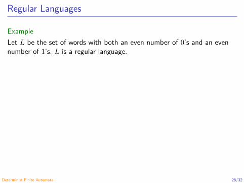
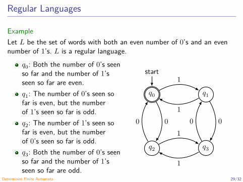
ExampleLet 𝐿 be the set of words with both an even number of 0’s and an evennumber of 1’s. 𝐿 is a regular language.
𝑞0: Both the number of 0’s seenso far and the number of 1’sseen so far are even.𝑞1: The number of 0’s seen sofar is even, but the numberof 1’s seen so far is odd.𝑞2: The number of 1’s seen sofar is even, but the numberof 0’s seen so far is odd.𝑞3: Both the number of 0’s seenso far and the number of 1’sseen so far are odd.
𝑞0
start
𝑞1
𝑞2 𝑞3
1
01
001
0
1
Determinist Finite Automata 28/32
Regular Languages
ExampleLet 𝐿 be the set of words with both an even number of 0’s and an evennumber of 1’s. 𝐿 is a regular language.
𝑞0: Both the number of 0’s seenso far and the number of 1’sseen so far are even.𝑞1: The number of 0’s seen sofar is even, but the numberof 1’s seen so far is odd.𝑞2: The number of 1’s seen sofar is even, but the numberof 0’s seen so far is odd.𝑞3: Both the number of 0’s seenso far and the number of 1’sseen so far are odd.
𝑞0
start
𝑞1
𝑞2 𝑞3
1
01
001
0
1Determinist Finite Automata 29/32

Functional Program View of Finite Automata
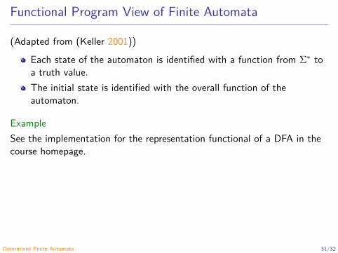
(Adapted from (Keller 2001))Each state of the automaton is identified with a function from Σ∗ toa truth value.The initial state is identified with the overall function of theautomaton.
ExampleSee the implementation for the representation functional of a DFA in thecourse homepage.
Determinist Finite Automata 30/32
Functional Program View of Finite Automata
(Adapted from (Keller 2001))Each state of the automaton is identified with a function from Σ∗ toa truth value.The initial state is identified with the overall function of theautomaton.
ExampleSee the implementation for the representation functional of a DFA in thecourse homepage.
Determinist Finite Automata 31/32

References
Greibach, S. A. (1981). Formal Languages: Origins and Directions. Annalsof History of Computing 3.1, pp. 14–41. doi: 10.1109/MAHC.1981.10006(cit. on p. 2).Hopcroft, J. E. and Ullman, J. D. (1979). Introduction to AutomataTheory, Languages, and Computation. Addison-Wesley Publishing Company(cit. on pp. 5, 7).Keller, R. M. (2001). Computer Science: Abstraction to Implementation.url: www.cs.hmc.edu/~keller/cs60book/ (visited on 07/02/2018) (cit. onpp. 30, 31).Levitin, A. (2006). Introduction to the Design and Analysis of Algorithms.2nd ed. Addison Wesley (cit. on p. 5).
Determinist Finite Automata 32/32
Automata and Formal Languages - CM0081Non-Deterministic Finite Automata
Andrés Sicard-Ramírez
Universidad EAFIT
Semester 2018-1

Non-Deterministic Finite Automata (NFA)
Introduction
𝑞𝑖
𝑞𝑗
𝑞𝑘
⋮
a
a
a
The automaton can be in several states at onceFacilitates the design of automata
Question: Are the NFAs more powerful than the DFAs?
Non-Deterministic Finite Automata 2/38
Non-Deterministic Finite Automata (NFA)
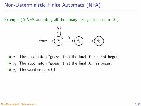
Example (A NFA accepting all the binary strings that end in 01)
𝑞0start 𝑞1 𝑞2
0, 1
0 1
𝑞0: The automaton “guess” that the final 01 has not begun.𝑞1: The automaton “guess” that the final 01 has begun.𝑞2: The word ends in 01.
Non-Deterministic Finite Automata 3/38
Definition
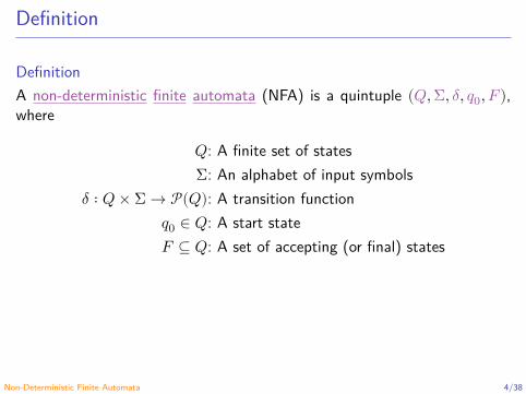
DefinitionA non-deterministic finite automata (NFA) is a quintuple (𝑄, Σ, 𝛿, 𝑞0, 𝐹 ),where
𝑄: A finite set of statesΣ: An alphabet of input symbols
𝛿 ∶ 𝑄 × Σ → 𝒫(𝑄): A transition function𝑞0 ∈ 𝑄: A start state𝐹 ⊆ 𝑄: A set of accepting (or final) states
Non-Deterministic Finite Automata 4/38

Extension of the Transition Function for NFAs
Let 𝑁 = (𝑄, Σ, 𝛿, 𝑞0, 𝐹 ) be a NFA. The extension of the transitionfunction, denoted by 𝛿, is recursively defined by
𝛿 ∶ 𝑄 × Σ∗ → 𝒫(𝑄)𝛿(𝑞, 𝜀) = {𝑞},
𝛿(𝑞, 𝑥𝑎) = ⋃𝑝∈ 𝛿(𝑞,𝑥)
𝛿(𝑝, 𝑎).
Non-Deterministic Finite Automata 5/38
Language Accepted by a NFA
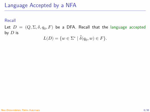
RecallLet 𝐷 = (𝑄, Σ, 𝛿, 𝑞0, 𝐹 ) be a DFA. Recall that the language acceptedby 𝐷 is
𝐿(𝐷) = {𝑤 ∈ Σ∗ ∣ 𝛿(𝑞0, 𝑤) ∈ 𝐹}.
DefinitionLet 𝑁 = (𝑄, Σ, 𝛿, 𝑞0, 𝐹 ) be a NFA. The language accepted by 𝑁 is
𝐿(𝑁) = {𝑤 ∈ Σ∗ ∣ 𝛿(𝑞0, 𝑤) ∩ 𝐹 ≠ ∅}.ReadingAn application: Text search (Hopcroft, Motwani and Ullman 2007, § 2.4).
Non-Deterministic Finite Automata 6/38

Language Accepted by a NFA
RecallLet 𝐷 = (𝑄, Σ, 𝛿, 𝑞0, 𝐹 ) be a DFA. Recall that the language acceptedby 𝐷 is
𝐿(𝐷) = {𝑤 ∈ Σ∗ ∣ 𝛿(𝑞0, 𝑤) ∈ 𝐹}.
DefinitionLet 𝑁 = (𝑄, Σ, 𝛿, 𝑞0, 𝐹 ) be a NFA. The language accepted by 𝑁 is
𝐿(𝑁) = {𝑤 ∈ Σ∗ ∣ 𝛿(𝑞0, 𝑤) ∩ 𝐹 ≠ ∅}.
ReadingAn application: Text search (Hopcroft, Motwani and Ullman 2007, § 2.4).
Non-Deterministic Finite Automata 7/38

Language Accepted by a NFA
RecallLet 𝐷 = (𝑄, Σ, 𝛿, 𝑞0, 𝐹 ) be a DFA. Recall that the language acceptedby 𝐷 is
𝐿(𝐷) = {𝑤 ∈ Σ∗ ∣ 𝛿(𝑞0, 𝑤) ∈ 𝐹}.
DefinitionLet 𝑁 = (𝑄, Σ, 𝛿, 𝑞0, 𝐹 ) be a NFA. The language accepted by 𝑁 is
𝐿(𝑁) = {𝑤 ∈ Σ∗ ∣ 𝛿(𝑞0, 𝑤) ∩ 𝐹 ≠ ∅}.ReadingAn application: Text search (Hopcroft, Motwani and Ullman 2007, § 2.4).
Non-Deterministic Finite Automata 8/38

Language Accepted by a NFA
Example (2.9)For the NFA of the figure, 𝐿(𝑁) = {𝑤 ∈ {0, 1}∗ ∣ 𝑤 ends in 01}.
𝑞0start 𝑞1 𝑞2
0, 1
0 1
Sketch of proofMutual induction on the following propositions:𝑆0(𝑤): 𝑞0 ∈ 𝛿(𝑞0, 𝑤) for all 𝑤 ∈ Σ∗
𝑆1(𝑤): 𝑞1 ∈ 𝛿(𝑞0, 𝑤) ⇔ 𝑤 ends in 0𝑆2(𝑤): 𝑞2 ∈ 𝛿(𝑞0, 𝑤) ⇔ 𝑤 ends in 01From 𝑆2(𝑤) and 𝐹 = {𝑞2} then the theorem follows.
Non-Deterministic Finite Automata 9/38

Language Accepted by a NFA
Example (2.9)For the NFA of the figure, 𝐿(𝑁) = {𝑤 ∈ {0, 1}∗ ∣ 𝑤 ends in 01}.
𝑞0start 𝑞1 𝑞2
0, 1
0 1
Sketch of proofMutual induction on the following propositions:𝑆0(𝑤): 𝑞0 ∈ 𝛿(𝑞0, 𝑤) for all 𝑤 ∈ Σ∗
𝑆1(𝑤): 𝑞1 ∈ 𝛿(𝑞0, 𝑤) ⇔ 𝑤 ends in 0𝑆2(𝑤): 𝑞2 ∈ 𝛿(𝑞0, 𝑤) ⇔ 𝑤 ends in 01From 𝑆2(𝑤) and 𝐹 = {𝑞2} then the theorem follows.
Non-Deterministic Finite Automata 10/38

Language Accepted by a NFA
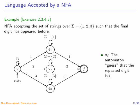
Example (Exercise 2.3.4.a)NFA accepting the set of strings over Σ = {1, 2, 3} such that the finaldigit has appeared before.
𝑖
start
𝑞2
𝑞1
𝑞3
𝑓
Σ 1
2
3
Σ − {1}
1Σ − {2}
2
Σ − {3} 3
𝑞𝑖: Theautomaton“guess” that therepeated digitis 𝑖.
Non-Deterministic Finite Automata 11/38
Language Accepted by a NFA
Example (Exercise 2.3.4.a)NFA accepting the set of strings over Σ = {1, 2, 3} such that the finaldigit has appeared before.
𝑖
start
𝑞2
𝑞1
𝑞3
𝑓
Σ 1
2
3
Σ − {1}
1Σ − {2}
2
Σ − {3} 3
𝑞𝑖: Theautomaton“guess” that therepeated digitis 𝑖.
Non-Deterministic Finite Automata 12/38

Language Accepted by a NFA
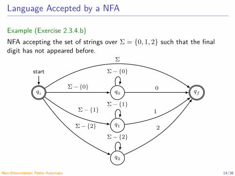
Example (Exercise 2.3.4.b)NFA accepting the set of strings over Σ = {0, 1, 2} such that the finaldigit has not appeared before.
𝑞0
𝑞1
𝑞2
𝑞𝑖
start
𝑞𝑓Σ − {0}
Σ − {1}
Σ − {2}
Σ
Σ − {0}
0
Σ − {1}1
Σ − {2}2
Non-Deterministic Finite Automata 13/38
Language Accepted by a NFA
Example (Exercise 2.3.4.b)NFA accepting the set of strings over Σ = {0, 1, 2} such that the finaldigit has not appeared before.
𝑞0
𝑞1
𝑞2
𝑞𝑖
start
𝑞𝑓Σ − {0}
Σ − {1}
Σ − {2}
Σ
Σ − {0}
0
Σ − {1}1
Σ − {2}2
Non-Deterministic Finite Automata 14/38

Language Accepted by a NFA
Example (Exercise 2.3.4.c)NFA accepting the set of strings over Σ = {0, 1} such that there aretwo 0’s separated by a number of positions that is multiple of 2. Notethat 0 is an allowable multiple of 2.
𝑞0
start
𝑞1 𝑞2
𝑞3 𝑞4 𝑞5 𝑞6
Σ
0
0
0
Σ
Σ Σ 0
1 Σ
Non-Deterministic Finite Automata 15/38

Language Accepted by a NFA
Example (Exercise 2.3.4.c)NFA accepting the set of strings over Σ = {0, 1} such that there aretwo 0’s separated by a number of positions that is multiple of 2. Notethat 0 is an allowable multiple of 2.
𝑞0
start
𝑞1 𝑞2
𝑞3 𝑞4 𝑞5 𝑞6
Σ
0
0
0
Σ
Σ Σ 0
1 Σ
Non-Deterministic Finite Automata 16/38
Language Accepted by a NFA
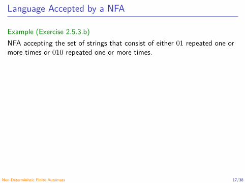
Example (Exercise 2.5.3.b)NFA accepting the set of strings that consist of either 01 repeated one ormore times or 010 repeated one or more times.
𝑞0
start
𝑞1 𝑞2
𝑞3 𝑞4 𝑞5
0
0
1
0
1 0
0
Non-Deterministic Finite Automata 17/38

Language Accepted by a NFA
Example (Exercise 2.5.3.b)NFA accepting the set of strings that consist of either 01 repeated one ormore times or 010 repeated one or more times.
𝑞0
start
𝑞1 𝑞2
𝑞3 𝑞4 𝑞5
0
0
1
0
1 0
0Non-Deterministic Finite Automata 18/38

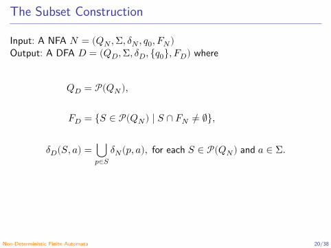
The Subset Construction
Input: A NFA 𝑁 = (𝑄𝑁 , Σ, 𝛿𝑁 , 𝑞0, 𝐹𝑁)Output: A DFA 𝐷 = (𝑄𝐷, Σ, 𝛿𝐷, {𝑞0}, 𝐹𝐷) where
𝑄𝐷 = 𝒫(𝑄𝑁),
𝐹𝐷 = {𝑆 ∈ 𝒫(𝑄𝑁) ∣ 𝑆 ∩ 𝐹𝑁 ≠ ∅},
𝛿𝐷(𝑆, 𝑎) = ⋃𝑝∈𝑆
𝛿𝑁(𝑝, 𝑎), for each 𝑆 ∈ 𝒫(𝑄𝑁) and 𝑎 ∈ Σ.
Non-Deterministic Finite Automata 19/38
The Subset Construction
Input: A NFA 𝑁 = (𝑄𝑁 , Σ, 𝛿𝑁 , 𝑞0, 𝐹𝑁)Output: A DFA 𝐷 = (𝑄𝐷, Σ, 𝛿𝐷, {𝑞0}, 𝐹𝐷) where
𝑄𝐷 = 𝒫(𝑄𝑁),
𝐹𝐷 = {𝑆 ∈ 𝒫(𝑄𝑁) ∣ 𝑆 ∩ 𝐹𝑁 ≠ ∅},
𝛿𝐷(𝑆, 𝑎) = ⋃𝑝∈𝑆
𝛿𝑁(𝑝, 𝑎), for each 𝑆 ∈ 𝒫(𝑄𝑁) and 𝑎 ∈ Σ.
Non-Deterministic Finite Automata 20/38
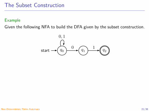
The Subset Construction
ExampleGiven the following NFA to build the DFA given by the subset construction.
𝑞0start 𝑞1 𝑞2
0, 1
0 1
Non-Deterministic Finite Automata 21/38

The Subset Construction
Example (cont.)
{𝑞0}
start
{𝑞0, 𝑞1} {𝑞0, 𝑞2}
{𝑞0, 𝑞1, 𝑞2} ∅ {𝑞1, 𝑞2}
{𝑞1} {𝑞2}
1
0
0
1
01
01
0, 1
0
1
0, 1
0
1
Non-Deterministic Finite Automata 22/38

The Subset Construction
Example (cont.)
{𝑞0}
start
{𝑞0, 𝑞1} {𝑞0, 𝑞2}
{𝑞0, 𝑞1, 𝑞2} ∅ {𝑞1, 𝑞2}
{𝑞1} {𝑞2}
1
0
0
1
01
01
0, 1
0
1
0, 1
0
1
Non-Deterministic Finite Automata 23/38

The Subset Construction
Example (cont.)
{𝑞0}start {𝑞0, 𝑞1} {𝑞0, 𝑞2}
1
0
0
1
01
Non-Deterministic Finite Automata 24/38
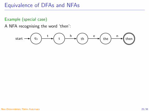
Equivalence of DFAs and NFAs
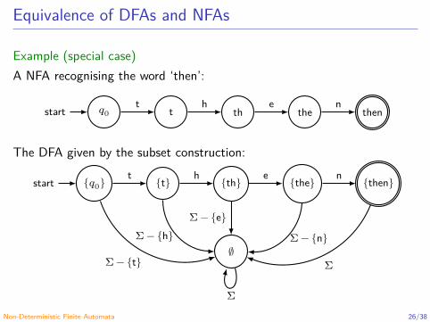
Example (special case)A NFA recognising the word ‘then’:
𝑞0start t th the thent h e n
The DFA given by the subset construction:
{𝑞0}start {t} {th} {the} {then}
∅
t
Σ − {t}
h
Σ − {h}
e
Σ − {e}
n
Σ − {n}
Σ
Σ
Non-Deterministic Finite Automata 25/38
Equivalence of DFAs and NFAs
Example (special case)A NFA recognising the word ‘then’:
𝑞0start t th the thent h e n
The DFA given by the subset construction:
{𝑞0}start {t} {th} {the} {then}
∅
t
Σ − {t}
h
Σ − {h}
e
Σ − {e}
n
Σ − {n}
Σ
ΣNon-Deterministic Finite Automata 26/38

Equivalence of DFAs and NFAs
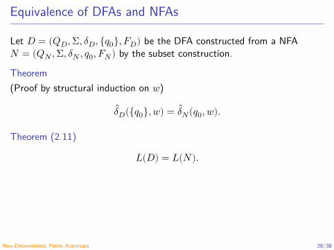
Let 𝐷 = (𝑄𝐷, Σ, 𝛿𝐷, {𝑞0}, 𝐹𝐷) be the DFA constructed from a NFA𝑁 = (𝑄𝑁 , Σ, 𝛿𝑁 , 𝑞0, 𝐹𝑁) by the subset construction.
Theorem(Proof by structural induction on 𝑤)
𝛿𝐷({𝑞0}, 𝑤) = 𝛿𝑁(𝑞0, 𝑤).
Theorem (2.11)
𝐿(𝐷) = 𝐿(𝑁).
Non-Deterministic Finite Automata 27/38
Equivalence of DFAs and NFAs
Let 𝐷 = (𝑄𝐷, Σ, 𝛿𝐷, {𝑞0}, 𝐹𝐷) be the DFA constructed from a NFA𝑁 = (𝑄𝑁 , Σ, 𝛿𝑁 , 𝑞0, 𝐹𝑁) by the subset construction.
Theorem(Proof by structural induction on 𝑤)
𝛿𝐷({𝑞0}, 𝑤) = 𝛿𝑁(𝑞0, 𝑤).
Theorem (2.11)
𝐿(𝐷) = 𝐿(𝑁).
Non-Deterministic Finite Automata 28/38
Equivalence of DFAs and NFAs
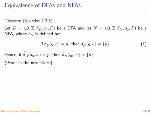
Theorem (Exercise 2.3.5)Let 𝐷 = (𝑄, Σ, 𝛿𝐷, 𝑞0, 𝐹 ) be a DFA and let 𝑁 = (𝑄, Σ, 𝛿𝑁 , 𝑞0, 𝐹 ) be aNFA, where 𝛿𝑁 is defined by:
if 𝛿𝐷(𝑞, 𝑎) = 𝑝, then 𝛿𝑁(𝑞, 𝑎) = {𝑝}. (1)
Hence, if 𝛿𝐷(𝑞0, 𝑤) = 𝑝, then 𝛿𝑁(𝑞0, 𝑤) = {𝑝}.(Proof in the next slides)
Non-Deterministic Finite Automata 29/38

Equivalence of DFAs and NFAs
Proof (by structural induction on 𝑤)
1. 𝑃(𝑤): If 𝛿𝐷(𝑞0, 𝑤) = 𝑝, then 𝛿𝑁(𝑞0, 𝑤) = {𝑝}.
2. Basis step 𝑃(𝜀):Since 𝛿𝐷(𝑞0, 𝜀) = 𝑞0 (by def. of 𝛿𝐷) and 𝛿𝑁(𝑞0, 𝜀) = {𝑞0} (by def.of 𝛿𝑁) then 𝑃(𝜀).
Non-Deterministic Finite Automata 30/38

Equivalence of DFAs and NFAs
Proof (by structural induction on 𝑤)
1. 𝑃(𝑤): If 𝛿𝐷(𝑞0, 𝑤) = 𝑝, then 𝛿𝑁(𝑞0, 𝑤) = {𝑝}.
2. Basis step 𝑃(𝜀):Since 𝛿𝐷(𝑞0, 𝜀) = 𝑞0 (by def. of 𝛿𝐷) and 𝛿𝑁(𝑞0, 𝜀) = {𝑞0} (by def.of 𝛿𝑁) then 𝑃(𝜀).
Non-Deterministic Finite Automata 31/38

Equivalence of DFAs and NFAs
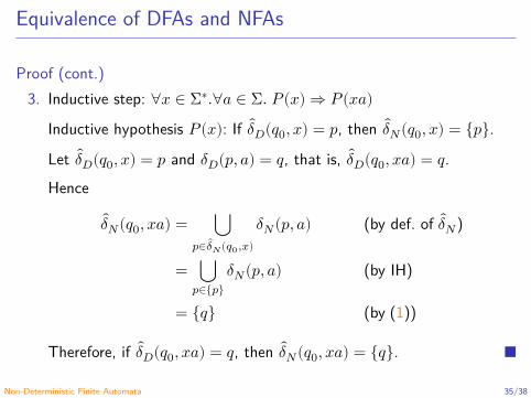
Proof (cont.)3. Inductive step: ∀𝑥 ∈ Σ∗.∀𝑎 ∈ Σ. 𝑃(𝑥) ⇒ 𝑃(𝑥𝑎)
Inductive hypothesis 𝑃(𝑥): If 𝛿𝐷(𝑞0, 𝑥) = 𝑝, then 𝛿𝑁(𝑞0, 𝑥) = {𝑝}.
Let 𝛿𝐷(𝑞0, 𝑥) = 𝑝 and 𝛿𝐷(𝑝, 𝑎) = 𝑞, that is, 𝛿𝐷(𝑞0, 𝑥𝑎) = 𝑞.Hence
𝛿𝑁(𝑞0, 𝑥𝑎) = ⋃𝑝∈ 𝛿𝑁(𝑞0,𝑥)
𝛿𝑁(𝑝, 𝑎) (by def. of 𝛿𝑁)
= ⋃𝑝∈{𝑝}
𝛿𝑁(𝑝, 𝑎) (by IH)
= {𝑞} (by (1))
Therefore, if 𝛿𝐷(𝑞0, 𝑥𝑎) = 𝑞, then 𝛿𝑁(𝑞0, 𝑥𝑎) = {𝑞}.
Non-Deterministic Finite Automata 32/38

Equivalence of DFAs and NFAs
Proof (cont.)3. Inductive step: ∀𝑥 ∈ Σ∗.∀𝑎 ∈ Σ. 𝑃(𝑥) ⇒ 𝑃(𝑥𝑎)
Inductive hypothesis 𝑃(𝑥): If 𝛿𝐷(𝑞0, 𝑥) = 𝑝, then 𝛿𝑁(𝑞0, 𝑥) = {𝑝}.
Let 𝛿𝐷(𝑞0, 𝑥) = 𝑝 and 𝛿𝐷(𝑝, 𝑎) = 𝑞, that is, 𝛿𝐷(𝑞0, 𝑥𝑎) = 𝑞.Hence
𝛿𝑁(𝑞0, 𝑥𝑎) = ⋃𝑝∈ 𝛿𝑁(𝑞0,𝑥)
𝛿𝑁(𝑝, 𝑎) (by def. of 𝛿𝑁)
= ⋃𝑝∈{𝑝}
𝛿𝑁(𝑝, 𝑎) (by IH)
= {𝑞} (by (1))
Therefore, if 𝛿𝐷(𝑞0, 𝑥𝑎) = 𝑞, then 𝛿𝑁(𝑞0, 𝑥𝑎) = {𝑞}.
Non-Deterministic Finite Automata 33/38

Equivalence of DFAs and NFAs
Proof (cont.)3. Inductive step: ∀𝑥 ∈ Σ∗.∀𝑎 ∈ Σ. 𝑃(𝑥) ⇒ 𝑃(𝑥𝑎)
Inductive hypothesis 𝑃(𝑥): If 𝛿𝐷(𝑞0, 𝑥) = 𝑝, then 𝛿𝑁(𝑞0, 𝑥) = {𝑝}.
Let 𝛿𝐷(𝑞0, 𝑥) = 𝑝 and 𝛿𝐷(𝑝, 𝑎) = 𝑞, that is, 𝛿𝐷(𝑞0, 𝑥𝑎) = 𝑞.
Hence
𝛿𝑁(𝑞0, 𝑥𝑎) = ⋃𝑝∈ 𝛿𝑁(𝑞0,𝑥)
𝛿𝑁(𝑝, 𝑎) (by def. of 𝛿𝑁)
= ⋃𝑝∈{𝑝}
𝛿𝑁(𝑝, 𝑎) (by IH)
= {𝑞} (by (1))
Therefore, if 𝛿𝐷(𝑞0, 𝑥𝑎) = 𝑞, then 𝛿𝑁(𝑞0, 𝑥𝑎) = {𝑞}.
Non-Deterministic Finite Automata 34/38
Equivalence of DFAs and NFAs
Proof (cont.)3. Inductive step: ∀𝑥 ∈ Σ∗.∀𝑎 ∈ Σ. 𝑃(𝑥) ⇒ 𝑃(𝑥𝑎)
Inductive hypothesis 𝑃(𝑥): If 𝛿𝐷(𝑞0, 𝑥) = 𝑝, then 𝛿𝑁(𝑞0, 𝑥) = {𝑝}.
Let 𝛿𝐷(𝑞0, 𝑥) = 𝑝 and 𝛿𝐷(𝑝, 𝑎) = 𝑞, that is, 𝛿𝐷(𝑞0, 𝑥𝑎) = 𝑞.Hence
𝛿𝑁(𝑞0, 𝑥𝑎) = ⋃𝑝∈ 𝛿𝑁(𝑞0,𝑥)
𝛿𝑁(𝑝, 𝑎) (by def. of 𝛿𝑁)
= ⋃𝑝∈{𝑝}
𝛿𝑁(𝑝, 𝑎) (by IH)
= {𝑞} (by (1))
Therefore, if 𝛿𝐷(𝑞0, 𝑥𝑎) = 𝑞, then 𝛿𝑁(𝑞0, 𝑥𝑎) = {𝑞}.
Non-Deterministic Finite Automata 35/38

Equivalence of DFAs and NFAs
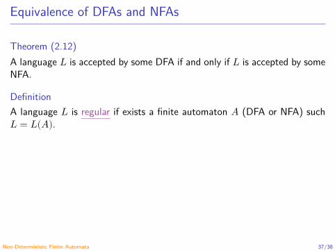
Theorem (2.12)A language 𝐿 is accepted by some DFA if and only if 𝐿 is accepted by someNFA.
DefinitionA language 𝐿 is regular if exists a finite automaton 𝐴 (DFA or NFA) such𝐿 = 𝐿(𝐴).
Non-Deterministic Finite Automata 36/38
Equivalence of DFAs and NFAs
Theorem (2.12)A language 𝐿 is accepted by some DFA if and only if 𝐿 is accepted by someNFA.
DefinitionA language 𝐿 is regular if exists a finite automaton 𝐴 (DFA or NFA) such𝐿 = 𝐿(𝐴).
Non-Deterministic Finite Automata 37/38
References
Hopcroft, J. E., Motwani, R. and Ullman, J. D. (2007). Introduction toAutomata theory, Languages, and Computation. 3rd ed. Pearson Education(cit. on pp. 6–8).
Non-Deterministic Finite Automata 38/38
Automata and Formal Languages - CM0081Finite Automata with 𝜀-Transitions
Andrés Sicard-Ramírez
Universidad EAFIT
Semester 2018-1

Finite Automata with 𝜀-Transitions (𝜀-NFA)
FeaturesTo allow a transition with 𝜀, the empty stringFacilitate the design of the automata
QuestionAre the 𝜀-NFAs more powerful than the [D|N]FAs?
Finite Automata with 𝜀-Transitions 2/16

Finite Automata with 𝜀-Transitions (𝜀-NFA)
FeaturesTo allow a transition with 𝜀, the empty stringFacilitate the design of the automata
QuestionAre the 𝜀-NFAs more powerful than the [D|N]FAs?
Finite Automata with 𝜀-Transitions 3/16
𝜀-NFA
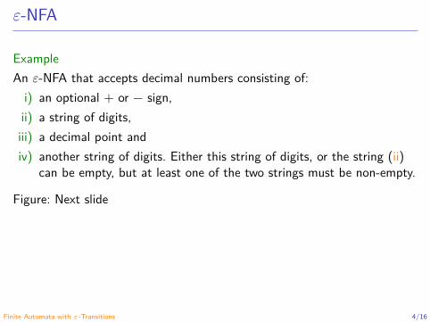
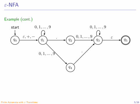
ExampleAn 𝜀-NFA that accepts decimal numbers consisting of:
i) an optional + or − sign,ii) a string of digits,iii) a decimal point andiv) another string of digits. Either this string of digits, or the string (ii)
can be empty, but at least one of the two strings must be non-empty.
Figure: Next slide
Finite Automata with 𝜀-Transitions 4/16
𝜀-NFA
Example (cont.)
𝑞0
start
𝑞1 𝑞2 𝑞3
𝑞4
𝑞5𝜀, +, −
0, 1, … , 9
.
0, 1, … , 9
0, 1, … , 9
0, 1, … , 9
𝜀
.
Finite Automata with 𝜀-Transitions 5/16

Definition
DefinitionA finite automata with 𝜀-transitions (𝜀-NFA) is a quintuple (𝑄, Σ, 𝛿, 𝑞0, 𝐹 ),where
𝑄: A finite set of statesΣ: An alphabet of input symbols
𝛿 → 𝑄 × Σ ∪ {𝜀} → 𝒫(𝑄): A transition function𝑞0 ∈ 𝑄: A start state𝐹 ⊆ 𝑄: A set of accepting (or final) states
Finite Automata with 𝜀-Transitions 6/16
Epsilon-Closures
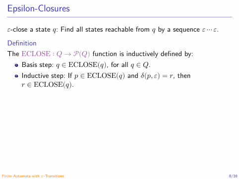
𝜀-close a state 𝑞: Find all states reachable from 𝑞 by a sequence 𝜀 ⋯ 𝜀.
DefinitionThe ECLOSE ∶ 𝑄 → 𝒫(𝑄) function is inductively defined by:
Basis step: 𝑞 ∈ ECLOSE(𝑞), for all 𝑞 ∈ 𝑄.Inductive step: If 𝑝 ∈ ECLOSE(𝑞) and 𝛿(𝑝, 𝜀) = 𝑟, then𝑟 ∈ ECLOSE(𝑞).
Example
1
2 3
4 5
6
7
𝜀
𝜀
𝜀 𝜀
a
b
𝜀
Finite Automata with 𝜀-Transitions 7/16
Epsilon-Closures
𝜀-close a state 𝑞: Find all states reachable from 𝑞 by a sequence 𝜀 ⋯ 𝜀.
DefinitionThe ECLOSE ∶ 𝑄 → 𝒫(𝑄) function is inductively defined by:
Basis step: 𝑞 ∈ ECLOSE(𝑞), for all 𝑞 ∈ 𝑄.Inductive step: If 𝑝 ∈ ECLOSE(𝑞) and 𝛿(𝑝, 𝜀) = 𝑟, then𝑟 ∈ ECLOSE(𝑞).
Example
1
2 3
4 5
6
7
𝜀
𝜀
𝜀 𝜀
a
b
𝜀
Finite Automata with 𝜀-Transitions 8/16

Epsilon-Closures
𝜀-close a state 𝑞: Find all states reachable from 𝑞 by a sequence 𝜀 ⋯ 𝜀.
DefinitionThe ECLOSE ∶ 𝑄 → 𝒫(𝑄) function is inductively defined by:
Basis step: 𝑞 ∈ ECLOSE(𝑞), for all 𝑞 ∈ 𝑄.Inductive step: If 𝑝 ∈ ECLOSE(𝑞) and 𝛿(𝑝, 𝜀) = 𝑟, then𝑟 ∈ ECLOSE(𝑞).
Example
1
2 3
4 5
6
7
𝜀
𝜀
𝜀 𝜀
a
b
𝜀
Finite Automata with 𝜀-Transitions 9/16

Epsilon-Closures
DefinitionLet 𝑆 be a set of states. The 𝜀-closure of 𝑆 is defined by
ECLOSE(𝑆) = ⋃𝑞∈𝑆
ECLOSE(𝑞).
Finite Automata with 𝜀-Transitions 10/16

Extension of the Transition Function for 𝜀-NFAs
Let 𝐸 = (𝑄, Σ, 𝛿, 𝑞0, 𝐹 ) be an 𝜀-NFA. The extension of the transitionfunction, 𝛿 ∶ 𝑄 × Σ∗ → 𝒫(𝑄) is recursively defined by
𝛿(𝑞, 𝜀) = ECLOSE(𝑞),𝛿(𝑞, 𝑥𝑎) = ECLOSE({𝑟1, 𝑟2, … , 𝑟𝑚}),
where
𝛿(𝑞, 𝑥) = {𝑝1, 𝑝2, … , 𝑝𝑘},𝑘
⋃𝑖=1
𝛿(𝑝𝑖, 𝑎) = {𝑟1, 𝑟2, … , 𝑟𝑚}.
Finite Automata with 𝜀-Transitions 11/16

Language Accepted by an 𝜀-NFA
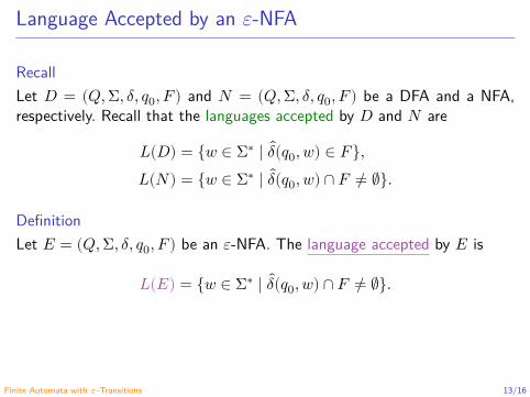
RecallLet 𝐷 = (𝑄, Σ, 𝛿, 𝑞0, 𝐹 ) and 𝑁 = (𝑄, Σ, 𝛿, 𝑞0, 𝐹 ) be a DFA and a NFA,respectively. Recall that the languages accepted by 𝐷 and 𝑁 are
𝐿(𝐷) = {𝑤 ∈ Σ∗ ∣ 𝛿(𝑞0, 𝑤) ∈ 𝐹},𝐿(𝑁) = {𝑤 ∈ Σ∗ ∣ 𝛿(𝑞0, 𝑤) ∩ 𝐹 ≠ ∅}.
DefinitionLet 𝐸 = (𝑄, Σ, 𝛿, 𝑞0, 𝐹 ) be an 𝜀-NFA. The language accepted by 𝐸 is
𝐿(𝐸) = {𝑤 ∈ Σ∗ ∣ 𝛿(𝑞0, 𝑤) ∩ 𝐹 ≠ ∅}.
Finite Automata with 𝜀-Transitions 12/16
Language Accepted by an 𝜀-NFA
RecallLet 𝐷 = (𝑄, Σ, 𝛿, 𝑞0, 𝐹 ) and 𝑁 = (𝑄, Σ, 𝛿, 𝑞0, 𝐹 ) be a DFA and a NFA,respectively. Recall that the languages accepted by 𝐷 and 𝑁 are
𝐿(𝐷) = {𝑤 ∈ Σ∗ ∣ 𝛿(𝑞0, 𝑤) ∈ 𝐹},𝐿(𝑁) = {𝑤 ∈ Σ∗ ∣ 𝛿(𝑞0, 𝑤) ∩ 𝐹 ≠ ∅}.
DefinitionLet 𝐸 = (𝑄, Σ, 𝛿, 𝑞0, 𝐹 ) be an 𝜀-NFA. The language accepted by 𝐸 is
𝐿(𝐸) = {𝑤 ∈ Σ∗ ∣ 𝛿(𝑞0, 𝑤) ∩ 𝐹 ≠ ∅}.
Finite Automata with 𝜀-Transitions 13/16
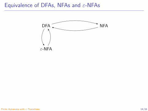
Equivalence of DFAs, NFAs and 𝜀-NFAs
DFA NFA
𝜀-NFA
Finite Automata with 𝜀-Transitions 14/16
Regular Languages
DefinitionA language 𝐿 is regular if exists a finite automaton 𝐴 (DFA, NFA or 𝜀-NFA)such 𝐿 = 𝐿(𝐴).
Exercise (2.5.3.a)Let 𝐿 be the set of strings consisting of zero or more 𝑎’s followed by zeroor more 𝑏’s, followed by zero or more 𝑐’s. Prove that 𝐿 is a regularlanguage.
Finite Automata with 𝜀-Transitions 15/16

Regular Languages
DefinitionA language 𝐿 is regular if exists a finite automaton 𝐴 (DFA, NFA or 𝜀-NFA)such 𝐿 = 𝐿(𝐴).
Exercise (2.5.3.a)Let 𝐿 be the set of strings consisting of zero or more 𝑎’s followed by zeroor more 𝑏’s, followed by zero or more 𝑐’s. Prove that 𝐿 is a regularlanguage.
Finite Automata with 𝜀-Transitions 16/16
Automata and Formal Languages - CM0081Regular Expressions
Andrés Sicard-Ramírez
Universidad EAFIT
Semester 2018-1
Introduction
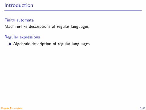
Finite automataMachine-like descriptions of regular languages.
Regular expressionsAlgebraic description of regular languagesDeclarative (“user-friendly”) way to express the strings that belong tothe languageExample: (01)(01)∗ + (010)(010)∗Uses
Search commands (e.g. Grep)Lexical-analyzer generators (e.g. Lex and Alex)Domain specific languages (DSLs)
Regular Expressions 2/40
Introduction
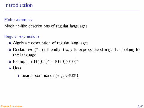
Finite automataMachine-like descriptions of regular languages.
Regular expressionsAlgebraic description of regular languages
Declarative (“user-friendly”) way to express the strings that belong tothe languageExample: (01)(01)∗ + (010)(010)∗Uses
Search commands (e.g. Grep)Lexical-analyzer generators (e.g. Lex and Alex)Domain specific languages (DSLs)
Regular Expressions 3/40

Introduction
Finite automataMachine-like descriptions of regular languages.
Regular expressionsAlgebraic description of regular languagesDeclarative (“user-friendly”) way to express the strings that belong tothe language
Example: (01)(01)∗ + (010)(010)∗Uses
Search commands (e.g. Grep)Lexical-analyzer generators (e.g. Lex and Alex)Domain specific languages (DSLs)
Regular Expressions 4/40

Introduction
Finite automataMachine-like descriptions of regular languages.
Regular expressionsAlgebraic description of regular languagesDeclarative (“user-friendly”) way to express the strings that belong tothe languageExample: (01)(01)∗ + (010)(010)∗
UsesSearch commands (e.g. Grep)Lexical-analyzer generators (e.g. Lex and Alex)Domain specific languages (DSLs)
Regular Expressions 5/40
Introduction
Finite automataMachine-like descriptions of regular languages.
Regular expressionsAlgebraic description of regular languagesDeclarative (“user-friendly”) way to express the strings that belong tothe languageExample: (01)(01)∗ + (010)(010)∗Uses
Search commands (e.g. Grep)
Lexical-analyzer generators (e.g. Lex and Alex)Domain specific languages (DSLs)
Regular Expressions 6/40
Introduction
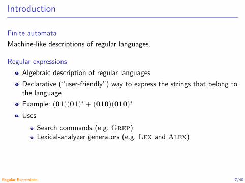
Finite automataMachine-like descriptions of regular languages.
Regular expressionsAlgebraic description of regular languagesDeclarative (“user-friendly”) way to express the strings that belong tothe languageExample: (01)(01)∗ + (010)(010)∗Uses
Search commands (e.g. Grep)Lexical-analyzer generators (e.g. Lex and Alex)
Domain specific languages (DSLs)
Regular Expressions 7/40

Introduction
Finite automataMachine-like descriptions of regular languages.
Regular expressionsAlgebraic description of regular languagesDeclarative (“user-friendly”) way to express the strings that belong tothe languageExample: (01)(01)∗ + (010)(010)∗Uses
Search commands (e.g. Grep)Lexical-analyzer generators (e.g. Lex and Alex)Domain specific languages (DSLs)
Regular Expressions 8/40

Operations on Languages
Let 𝐿 and 𝑀 be languages:
Union 𝐿 ∪𝑀 = {𝑤 ∣ 𝑤 ∈ 𝐿 or 𝑤 ∈ 𝑀}
Concatenation 𝐿.𝑀 = {𝑤 ∣ 𝑤 = 𝑥𝑦, 𝑥 ∈ 𝐿 and 𝑦 ∈ 𝑀}
Powers 𝐿0 = {𝜀}𝐿1 = 𝐿
𝐿𝑘+1 = 𝐿.𝐿𝑘
Kleene closure 𝐿∗ =∞⋃𝑖=0
𝐿𝑖
Regular Expressions 9/40
Operations on Languages
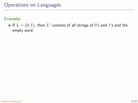
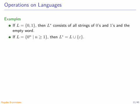
ExamplesIf 𝐿 = {0, 1}, then 𝐿∗ consists of all strings of 0’s and 1’s and theempty word.
If 𝐿 = {0𝑛 ∣ 𝑛 ≥ 1}, then 𝐿∗ = 𝐿 ∪ {𝜀}.If 𝐿 = {0, 11}, then 𝐿∗ consists of the empty word and those stringsof 0’s and 1’s such that the 1’s come in pairs.∅0 = {𝜀}∅𝑖 = ∅, for 𝑖 ≥ 1∅∗ = {𝜀}
Regular Expressions 10/40
Operations on Languages
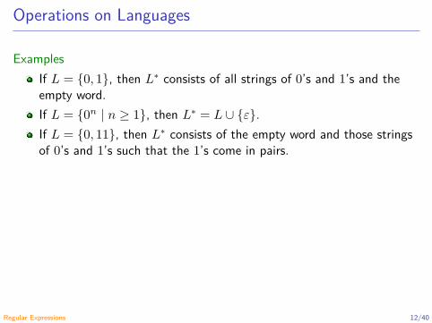
ExamplesIf 𝐿 = {0, 1}, then 𝐿∗ consists of all strings of 0’s and 1’s and theempty word.If 𝐿 = {0𝑛 ∣ 𝑛 ≥ 1}, then 𝐿∗ = 𝐿 ∪ {𝜀}.
If 𝐿 = {0, 11}, then 𝐿∗ consists of the empty word and those stringsof 0’s and 1’s such that the 1’s come in pairs.∅0 = {𝜀}∅𝑖 = ∅, for 𝑖 ≥ 1∅∗ = {𝜀}
Regular Expressions 11/40
Operations on Languages
ExamplesIf 𝐿 = {0, 1}, then 𝐿∗ consists of all strings of 0’s and 1’s and theempty word.If 𝐿 = {0𝑛 ∣ 𝑛 ≥ 1}, then 𝐿∗ = 𝐿 ∪ {𝜀}.If 𝐿 = {0, 11}, then 𝐿∗ consists of the empty word and those stringsof 0’s and 1’s such that the 1’s come in pairs.
∅0 = {𝜀}∅𝑖 = ∅, for 𝑖 ≥ 1∅∗ = {𝜀}
Regular Expressions 12/40

Operations on Languages
ExamplesIf 𝐿 = {0, 1}, then 𝐿∗ consists of all strings of 0’s and 1’s and theempty word.If 𝐿 = {0𝑛 ∣ 𝑛 ≥ 1}, then 𝐿∗ = 𝐿 ∪ {𝜀}.If 𝐿 = {0, 11}, then 𝐿∗ consists of the empty word and those stringsof 0’s and 1’s such that the 1’s come in pairs.∅0 = {𝜀}∅𝑖 = ∅, for 𝑖 ≥ 1∅∗ = {𝜀}
Regular Expressions 13/40

Syntax: What the Regular Expressions Are
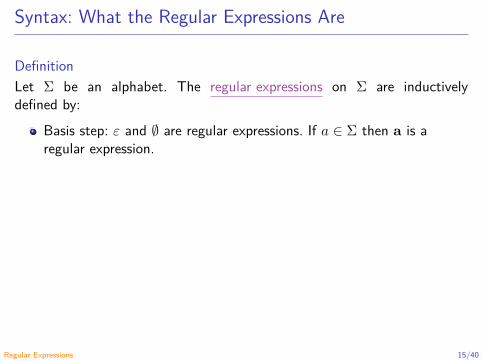
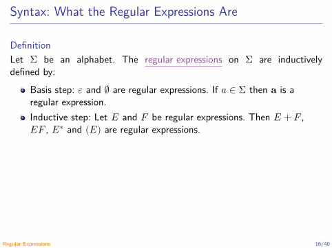
DefinitionLet Σ be an alphabet. The regular expressions on Σ are inductivelydefined by:
Basis step: 𝜀 and ∅ are regular expressions. If 𝑎 ∈ Σ then a is aregular expression.Inductive step: Let 𝐸 and 𝐹 be regular expressions. Then 𝐸 + 𝐹 ,𝐸𝐹 , 𝐸∗ and (𝐸) are regular expressions.
Regular Expressions 14/40
Syntax: What the Regular Expressions Are
DefinitionLet Σ be an alphabet. The regular expressions on Σ are inductivelydefined by:
Basis step: 𝜀 and ∅ are regular expressions. If 𝑎 ∈ Σ then a is aregular expression.
Inductive step: Let 𝐸 and 𝐹 be regular expressions. Then 𝐸 + 𝐹 ,𝐸𝐹 , 𝐸∗ and (𝐸) are regular expressions.
Regular Expressions 15/40
Syntax: What the Regular Expressions Are
DefinitionLet Σ be an alphabet. The regular expressions on Σ are inductivelydefined by:
Basis step: 𝜀 and ∅ are regular expressions. If 𝑎 ∈ Σ then a is aregular expression.Inductive step: Let 𝐸 and 𝐹 be regular expressions. Then 𝐸 + 𝐹 ,𝐸𝐹 , 𝐸∗ and (𝐸) are regular expressions.
Regular Expressions 16/40

Semantics: What Language Denotes a Regular Expression
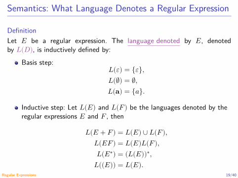
DefinitionLet 𝐸 be a regular expression. The language denoted by 𝐸, denotedby 𝐿(𝐷), is inductively defined by:
Basis step:𝐿(𝜀) = {𝜀},𝐿(∅) = ∅,𝐿(a) = {𝑎}.
Inductive step: Let 𝐿(𝐸) and 𝐿(𝐹) be the languages denoted by theregular expressions 𝐸 and 𝐹 , then
𝐿(𝐸 + 𝐹) = 𝐿(𝐸) ∪ 𝐿(𝐹),𝐿(𝐸𝐹) = 𝐿(𝐸)𝐿(𝐹),𝐿(𝐸∗) = (𝐿(𝐸))∗,𝐿((𝐸)) = 𝐿(𝐸).
Regular Expressions 17/40

Semantics: What Language Denotes a Regular Expression
DefinitionLet 𝐸 be a regular expression. The language denoted by 𝐸, denotedby 𝐿(𝐷), is inductively defined by:
Basis step:𝐿(𝜀) = {𝜀},𝐿(∅) = ∅,𝐿(a) = {𝑎}.
Inductive step: Let 𝐿(𝐸) and 𝐿(𝐹) be the languages denoted by theregular expressions 𝐸 and 𝐹 , then
𝐿(𝐸 + 𝐹) = 𝐿(𝐸) ∪ 𝐿(𝐹),𝐿(𝐸𝐹) = 𝐿(𝐸)𝐿(𝐹),𝐿(𝐸∗) = (𝐿(𝐸))∗,𝐿((𝐸)) = 𝐿(𝐸).
Regular Expressions 18/40
Semantics: What Language Denotes a Regular Expression
DefinitionLet 𝐸 be a regular expression. The language denoted by 𝐸, denotedby 𝐿(𝐷), is inductively defined by:
Basis step:𝐿(𝜀) = {𝜀},𝐿(∅) = ∅,𝐿(a) = {𝑎}.
Inductive step: Let 𝐿(𝐸) and 𝐿(𝐹) be the languages denoted by theregular expressions 𝐸 and 𝐹 , then
𝐿(𝐸 + 𝐹) = 𝐿(𝐸) ∪ 𝐿(𝐹),𝐿(𝐸𝐹) = 𝐿(𝐸)𝐿(𝐹),𝐿(𝐸∗) = (𝐿(𝐸))∗,𝐿((𝐸)) = 𝐿(𝐸).
Regular Expressions 19/40

Precedence of Operators
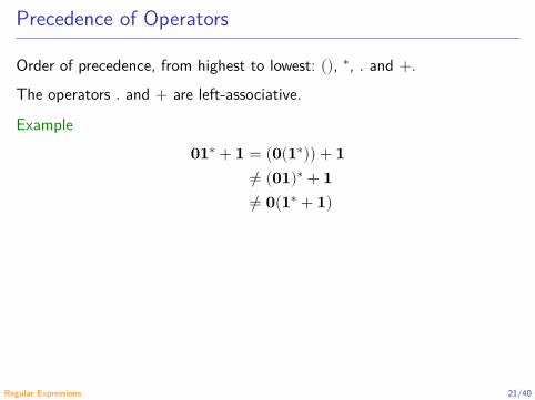
Order of precedence, from highest to lowest: (), ∗, . and +.The operators . and + are left-associative.
Example01∗ + 1 = (0(1∗)) + 1
≠ (01)∗ + 1≠ 0(1∗ + 1)
Regular Expressions 20/40
Precedence of Operators
Order of precedence, from highest to lowest: (), ∗, . and +.The operators . and + are left-associative.
Example01∗ + 1 = (0(1∗)) + 1
≠ (01)∗ + 1≠ 0(1∗ + 1)
Regular Expressions 21/40
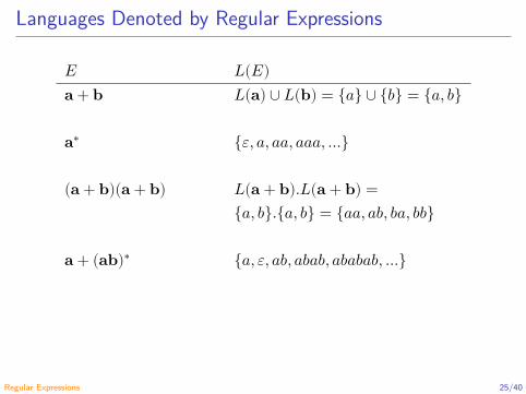
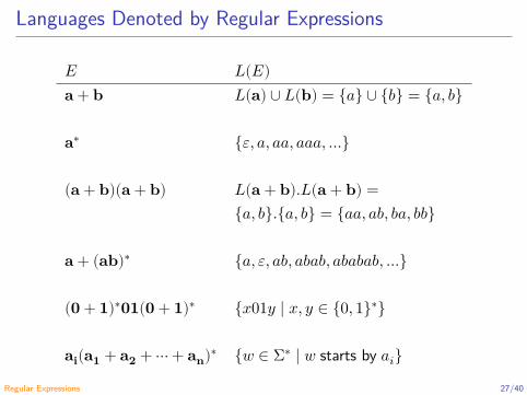
Languages Denoted by Regular Expressions
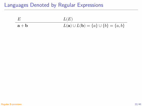
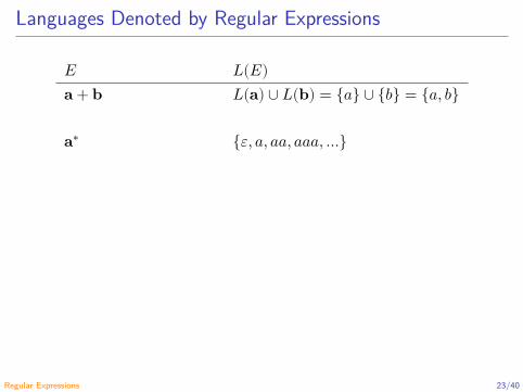
𝐸 𝐿(𝐸)a + b 𝐿(a) ∪ 𝐿(b) = {𝑎} ∪ {𝑏} = {𝑎, 𝑏}
a∗ {𝜀, 𝑎, 𝑎𝑎, 𝑎𝑎𝑎,…}
(a + b)(a + b) 𝐿(a + b).𝐿(a + b) ={𝑎, 𝑏}.{𝑎, 𝑏} = {𝑎𝑎, 𝑎𝑏, 𝑏𝑎, 𝑏𝑏}
a + (ab)∗ {𝑎, 𝜀, 𝑎𝑏, 𝑎𝑏𝑎𝑏, 𝑎𝑏𝑎𝑏𝑎𝑏,…}
(0 + 1)∗01(0 + 1)∗ {𝑥01𝑦 ∣ 𝑥, 𝑦 ∈ {0, 1}∗}
ai(a1 + a2 +⋯+ an)∗ {𝑤 ∈ Σ∗ ∣ 𝑤 starts by 𝑎𝑖}
Regular Expressions 22/40
Languages Denoted by Regular Expressions
𝐸 𝐿(𝐸)a + b 𝐿(a) ∪ 𝐿(b) = {𝑎} ∪ {𝑏} = {𝑎, 𝑏}
a∗ {𝜀, 𝑎, 𝑎𝑎, 𝑎𝑎𝑎,…}
(a + b)(a + b) 𝐿(a + b).𝐿(a + b) ={𝑎, 𝑏}.{𝑎, 𝑏} = {𝑎𝑎, 𝑎𝑏, 𝑏𝑎, 𝑏𝑏}
a + (ab)∗ {𝑎, 𝜀, 𝑎𝑏, 𝑎𝑏𝑎𝑏, 𝑎𝑏𝑎𝑏𝑎𝑏,…}
(0 + 1)∗01(0 + 1)∗ {𝑥01𝑦 ∣ 𝑥, 𝑦 ∈ {0, 1}∗}
ai(a1 + a2 +⋯+ an)∗ {𝑤 ∈ Σ∗ ∣ 𝑤 starts by 𝑎𝑖}
Regular Expressions 23/40

Languages Denoted by Regular Expressions
𝐸 𝐿(𝐸)a + b 𝐿(a) ∪ 𝐿(b) = {𝑎} ∪ {𝑏} = {𝑎, 𝑏}
a∗ {𝜀, 𝑎, 𝑎𝑎, 𝑎𝑎𝑎,…}
(a + b)(a + b) 𝐿(a + b).𝐿(a + b) ={𝑎, 𝑏}.{𝑎, 𝑏} = {𝑎𝑎, 𝑎𝑏, 𝑏𝑎, 𝑏𝑏}
a + (ab)∗ {𝑎, 𝜀, 𝑎𝑏, 𝑎𝑏𝑎𝑏, 𝑎𝑏𝑎𝑏𝑎𝑏,…}
(0 + 1)∗01(0 + 1)∗ {𝑥01𝑦 ∣ 𝑥, 𝑦 ∈ {0, 1}∗}
ai(a1 + a2 +⋯+ an)∗ {𝑤 ∈ Σ∗ ∣ 𝑤 starts by 𝑎𝑖}
Regular Expressions 24/40
Languages Denoted by Regular Expressions
𝐸 𝐿(𝐸)a + b 𝐿(a) ∪ 𝐿(b) = {𝑎} ∪ {𝑏} = {𝑎, 𝑏}
a∗ {𝜀, 𝑎, 𝑎𝑎, 𝑎𝑎𝑎,…}
(a + b)(a + b) 𝐿(a + b).𝐿(a + b) ={𝑎, 𝑏}.{𝑎, 𝑏} = {𝑎𝑎, 𝑎𝑏, 𝑏𝑎, 𝑏𝑏}
a + (ab)∗ {𝑎, 𝜀, 𝑎𝑏, 𝑎𝑏𝑎𝑏, 𝑎𝑏𝑎𝑏𝑎𝑏,…}
(0 + 1)∗01(0 + 1)∗ {𝑥01𝑦 ∣ 𝑥, 𝑦 ∈ {0, 1}∗}
ai(a1 + a2 +⋯+ an)∗ {𝑤 ∈ Σ∗ ∣ 𝑤 starts by 𝑎𝑖}
Regular Expressions 25/40

Languages Denoted by Regular Expressions
𝐸 𝐿(𝐸)a + b 𝐿(a) ∪ 𝐿(b) = {𝑎} ∪ {𝑏} = {𝑎, 𝑏}
a∗ {𝜀, 𝑎, 𝑎𝑎, 𝑎𝑎𝑎,…}
(a + b)(a + b) 𝐿(a + b).𝐿(a + b) ={𝑎, 𝑏}.{𝑎, 𝑏} = {𝑎𝑎, 𝑎𝑏, 𝑏𝑎, 𝑏𝑏}
a + (ab)∗ {𝑎, 𝜀, 𝑎𝑏, 𝑎𝑏𝑎𝑏, 𝑎𝑏𝑎𝑏𝑎𝑏,…}
(0 + 1)∗01(0 + 1)∗ {𝑥01𝑦 ∣ 𝑥, 𝑦 ∈ {0, 1}∗}
ai(a1 + a2 +⋯+ an)∗ {𝑤 ∈ Σ∗ ∣ 𝑤 starts by 𝑎𝑖}
Regular Expressions 26/40
Languages Denoted by Regular Expressions
𝐸 𝐿(𝐸)a + b 𝐿(a) ∪ 𝐿(b) = {𝑎} ∪ {𝑏} = {𝑎, 𝑏}
a∗ {𝜀, 𝑎, 𝑎𝑎, 𝑎𝑎𝑎,…}
(a + b)(a + b) 𝐿(a + b).𝐿(a + b) ={𝑎, 𝑏}.{𝑎, 𝑏} = {𝑎𝑎, 𝑎𝑏, 𝑏𝑎, 𝑏𝑏}
a + (ab)∗ {𝑎, 𝜀, 𝑎𝑏, 𝑎𝑏𝑎𝑏, 𝑎𝑏𝑎𝑏𝑎𝑏,…}
(0 + 1)∗01(0 + 1)∗ {𝑥01𝑦 ∣ 𝑥, 𝑦 ∈ {0, 1}∗}
ai(a1 + a2 +⋯+ an)∗ {𝑤 ∈ Σ∗ ∣ 𝑤 starts by 𝑎𝑖}Regular Expressions 27/40

Languages Denoted by Regular Expressions
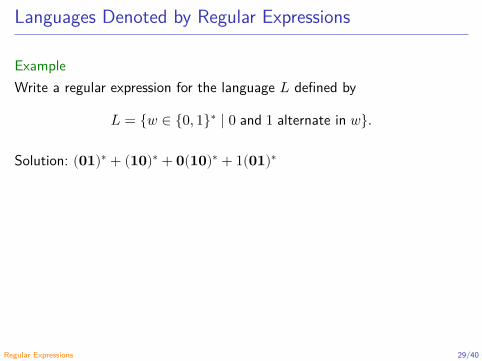
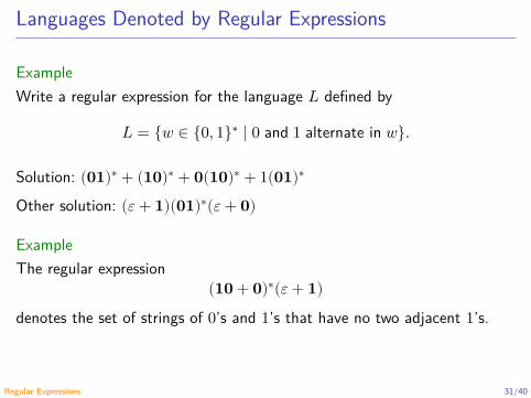
ExampleWrite a regular expression for the language 𝐿 defined by
𝐿 = {𝑤 ∈ {0, 1}∗ ∣ 0 and 1 alternate in 𝑤}.
Solution: (01)∗ + (10)∗ + 0(10)∗ + 1(01)∗
Other solution: (𝜀 + 1)(01)∗(𝜀 + 0)
ExampleThe regular expression
(10 + 0)∗(𝜀 + 1)denotes the set of strings of 0’s and 1’s that have no two adjacent 1’s.
Regular Expressions 28/40
Languages Denoted by Regular Expressions
ExampleWrite a regular expression for the language 𝐿 defined by
𝐿 = {𝑤 ∈ {0, 1}∗ ∣ 0 and 1 alternate in 𝑤}.
Solution: (01)∗ + (10)∗ + 0(10)∗ + 1(01)∗
Other solution: (𝜀 + 1)(01)∗(𝜀 + 0)
ExampleThe regular expression
(10 + 0)∗(𝜀 + 1)denotes the set of strings of 0’s and 1’s that have no two adjacent 1’s.
Regular Expressions 29/40

Languages Denoted by Regular Expressions
ExampleWrite a regular expression for the language 𝐿 defined by
𝐿 = {𝑤 ∈ {0, 1}∗ ∣ 0 and 1 alternate in 𝑤}.
Solution: (01)∗ + (10)∗ + 0(10)∗ + 1(01)∗
Other solution: (𝜀 + 1)(01)∗(𝜀 + 0)
ExampleThe regular expression
(10 + 0)∗(𝜀 + 1)denotes the set of strings of 0’s and 1’s that have no two adjacent 1’s.
Regular Expressions 30/40
Languages Denoted by Regular Expressions
ExampleWrite a regular expression for the language 𝐿 defined by
𝐿 = {𝑤 ∈ {0, 1}∗ ∣ 0 and 1 alternate in 𝑤}.
Solution: (01)∗ + (10)∗ + 0(10)∗ + 1(01)∗
Other solution: (𝜀 + 1)(01)∗(𝜀 + 0)
ExampleThe regular expression
(10 + 0)∗(𝜀 + 1)denotes the set of strings of 0’s and 1’s that have no two adjacent 1’s.
Regular Expressions 31/40
Languages Denoted by Regular Expressions
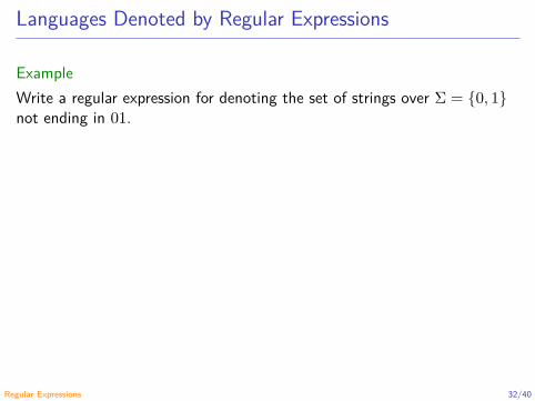
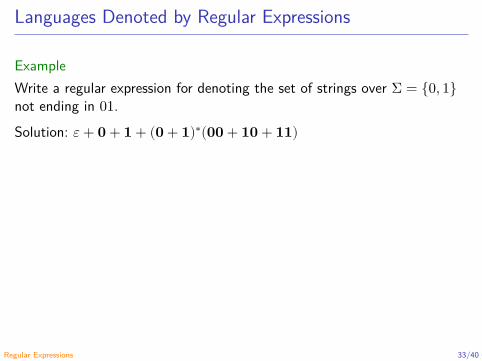
ExampleWrite a regular expression for denoting the set of strings over Σ = {0, 1}not ending in 01.
Solution: 𝜀 + 0 + 1 + (0 + 1)∗(00 + 10 + 11)
Regular Expressions 32/40
Languages Denoted by Regular Expressions
ExampleWrite a regular expression for denoting the set of strings over Σ = {0, 1}not ending in 01.Solution: 𝜀 + 0 + 1 + (0 + 1)∗(00 + 10 + 11)
Regular Expressions 33/40
Libraries
Note: Theoretical regular expressions ≠ practical regular expressions.
Some programming languages with support to regular expressions.NET, C, Haskell, Java, Mathematica, MATLAB and Perl.
Regular Expressions 34/40

Libraries
Note: Theoretical regular expressions ≠ practical regular expressions.
Some programming languages with support to regular expressions.NET, C, Haskell, Java, Mathematica, MATLAB and Perl.
Regular Expressions 35/40
Algorithms
AlgorithmsSee the Haskell implementation of some algorithms on regular expressionsin the course homepage.
Regular Expressions 36/40
Applications
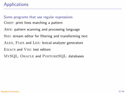
Some programs that use regular expressionsGrep: print lines matching a patternAwk: pattern scanning and processing languageSed: stream editor for filtering and transforming textAlex, Flex and Lex: lexical-analyzer generatorsEmacs and Vim: test editorsMySQL, Oracle and PostgreSQL: databases
Regular Expressions 37/40

Applications
ReadingApplications of Regular Expressions (Hopcroft, Motwani and Ullman 2007,§ 3.3).
𝐿+ def= 𝐿𝐿∗ (one or many times operator)
𝐿? def= 𝜀 + 𝐿 (zero or one time operator)
Regular Expressions 38/40
An Implementation: A Regular Expression Matcher
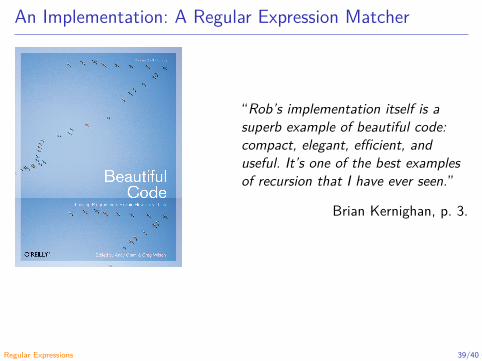
“Rob’s implementation itself is asuperb example of beautiful code:compact, elegant, efficient, anduseful. It’s one of the best examplesof recursion that I have ever seen.”
Brian Kernighan, p. 3.
Regular Expressions 39/40

References
Hopcroft, J. E., Motwani, R. and Ullman, J. D. (2007). Introduction toAutomata theory, Languages, and Computation. 3rd ed. Pearson Education(cit. on p. 38).
Regular Expressions 40/40
Automata and Formal Languages - CM0081Finite Automata and Regular Expressions
Andrés Sicard-Ramírez
Universidad EAFIT
Semester 2018-1
Introduction
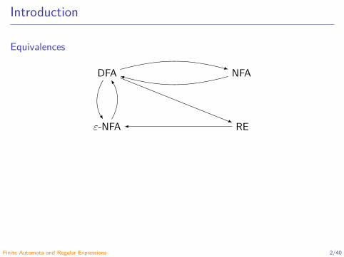
Equivalences
DFA NFA
𝜀-NFA RE
Finite Automata and Regular Expressions 2/40

From Finite Automata to Regular Expressions
Theorem (3.4)If 𝐿 = 𝐿(𝐷) for some DFA 𝐷, then there is a regular expression 𝑅 suchthat 𝐿 = 𝐿(𝑅).
Finite Automata and Regular Expressions 3/40

From Finite Automata to Regular Expressions
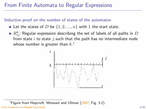
Inductive proof on the number of states of the automatonLet the states of 𝐷 be {1, 2, … , 𝑛} with 1 the start state.
𝑅𝑘𝑖𝑗: Regular expression describing the set of labels of all paths in 𝐷
from state 𝑖 to state 𝑗 such that the path has no intermediate nodewhose number is greater than 𝑘.†
†Figure from Hopcroft, Motwani and Ullman (2007, Fig. 3.2).Finite Automata and Regular Expressions 4/40
From Finite Automata to Regular Expressions
Inductive proof on the number of states of the automatonLet the states of 𝐷 be {1, 2, … , 𝑛} with 1 the start state.𝑅𝑘
𝑖𝑗: Regular expression describing the set of labels of all paths in 𝐷from state 𝑖 to state 𝑗 such that the path has no intermediate nodewhose number is greater than 𝑘.†
†Figure from Hopcroft, Motwani and Ullman (2007, Fig. 3.2).Finite Automata and Regular Expressions 5/40
From Finite Automata to Regular Expressions
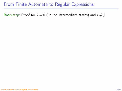
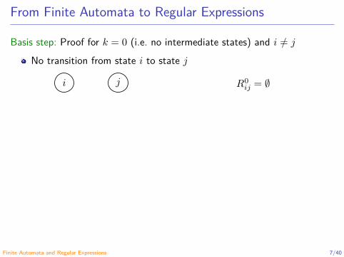
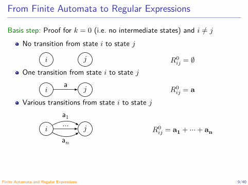
Basis step: Proof for 𝑘 = 0 (i.e. no intermediate states) and 𝑖 ≠ 𝑗
No transition from state 𝑖 to state 𝑗
𝑖 𝑗 𝑅0𝑖𝑗 = ∅
One transition from state 𝑖 to state 𝑗
𝑖 𝑗a 𝑅0𝑖𝑗 = a
Various transitions from state 𝑖 to state 𝑗
𝑖 𝑗a1…
a𝑛
𝑅0𝑖𝑗 = a1 + ⋯ + an
Finite Automata and Regular Expressions 6/40
From Finite Automata to Regular Expressions
Basis step: Proof for 𝑘 = 0 (i.e. no intermediate states) and 𝑖 ≠ 𝑗No transition from state 𝑖 to state 𝑗
𝑖 𝑗 𝑅0𝑖𝑗 = ∅
One transition from state 𝑖 to state 𝑗
𝑖 𝑗a 𝑅0𝑖𝑗 = a
Various transitions from state 𝑖 to state 𝑗
𝑖 𝑗a1…
a𝑛
𝑅0𝑖𝑗 = a1 + ⋯ + an
Finite Automata and Regular Expressions 7/40

From Finite Automata to Regular Expressions
Basis step: Proof for 𝑘 = 0 (i.e. no intermediate states) and 𝑖 ≠ 𝑗No transition from state 𝑖 to state 𝑗
𝑖 𝑗 𝑅0𝑖𝑗 = ∅
One transition from state 𝑖 to state 𝑗
𝑖 𝑗a 𝑅0𝑖𝑗 = a
Various transitions from state 𝑖 to state 𝑗
𝑖 𝑗a1…
a𝑛
𝑅0𝑖𝑗 = a1 + ⋯ + an
Finite Automata and Regular Expressions 8/40
From Finite Automata to Regular Expressions
Basis step: Proof for 𝑘 = 0 (i.e. no intermediate states) and 𝑖 ≠ 𝑗No transition from state 𝑖 to state 𝑗
𝑖 𝑗 𝑅0𝑖𝑗 = ∅
One transition from state 𝑖 to state 𝑗
𝑖 𝑗a 𝑅0𝑖𝑗 = a
Various transitions from state 𝑖 to state 𝑗
𝑖 𝑗a1…
a𝑛
𝑅0𝑖𝑗 = a1 + ⋯ + an
Finite Automata and Regular Expressions 9/40
From Finite Automata to Regular Expressions
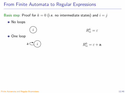
Basis step: Proof for 𝑘 = 0 (i.e. no intermediate states) and 𝑖 = 𝑗
No loops
𝑖 𝑅0𝑖𝑖 = 𝜀
One loop
𝑖a 𝑅0𝑖𝑖 = 𝜀 + a
Question: Why do not to define 𝑅0𝑖𝑖 = a∗ ?
Various loops
𝑖a1
…
a𝑛𝑅0
𝑖𝑖 = 𝜀 + a1 + ⋯ + an
Finite Automata and Regular Expressions 10/40

From Finite Automata to Regular Expressions
Basis step: Proof for 𝑘 = 0 (i.e. no intermediate states) and 𝑖 = 𝑗No loops
𝑖 𝑅0𝑖𝑖 = 𝜀
One loop
𝑖a 𝑅0𝑖𝑖 = 𝜀 + a
Question: Why do not to define 𝑅0𝑖𝑖 = a∗ ?
Various loops
𝑖a1
…
a𝑛𝑅0
𝑖𝑖 = 𝜀 + a1 + ⋯ + an
Finite Automata and Regular Expressions 11/40
From Finite Automata to Regular Expressions
Basis step: Proof for 𝑘 = 0 (i.e. no intermediate states) and 𝑖 = 𝑗No loops
𝑖 𝑅0𝑖𝑖 = 𝜀
One loop
𝑖a 𝑅0𝑖𝑖 = 𝜀 + a
Question: Why do not to define 𝑅0𝑖𝑖 = a∗ ?
Various loops
𝑖a1
…
a𝑛𝑅0
𝑖𝑖 = 𝜀 + a1 + ⋯ + an
Finite Automata and Regular Expressions 12/40

From Finite Automata to Regular Expressions
Basis step: Proof for 𝑘 = 0 (i.e. no intermediate states) and 𝑖 = 𝑗No loops
𝑖 𝑅0𝑖𝑖 = 𝜀
One loop
𝑖a 𝑅0𝑖𝑖 = 𝜀 + a
Question: Why do not to define 𝑅0𝑖𝑖 = a∗ ?
Various loops
𝑖a1
…
a𝑛𝑅0
𝑖𝑖 = 𝜀 + a1 + ⋯ + an
Finite Automata and Regular Expressions 13/40

From Finite Automata to Regular Expressions
Basis step: Proof for 𝑘 = 0 (i.e. no intermediate states) and 𝑖 = 𝑗No loops
𝑖 𝑅0𝑖𝑖 = 𝜀
One loop
𝑖a 𝑅0𝑖𝑖 = 𝜀 + a
Question: Why do not to define 𝑅0𝑖𝑖 = a∗ ?
Various loops
𝑖a1
…
a𝑛𝑅0
𝑖𝑖 = 𝜀 + a1 + ⋯ + an
Finite Automata and Regular Expressions 14/40
From Finite Automata to Regular Expressions
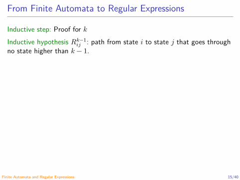
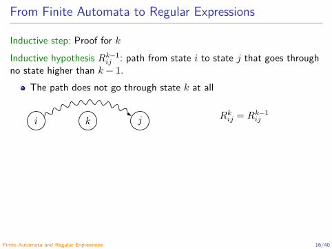
Inductive step: Proof for 𝑘Inductive hypothesis 𝑅𝑘−1
𝑖𝑗 : path from state 𝑖 to state 𝑗 that goes throughno state higher than 𝑘 − 1.
The path does not go through state 𝑘 at all
𝑖 𝑘 𝑗 𝑅𝑘𝑖𝑗 = 𝑅𝑘−1
𝑖𝑗
The path goes through state 𝑘 at least once
𝑖 𝑘 𝑘 𝑘 𝑗𝑅𝑘
𝑖𝑗 = 𝑅𝑘−1𝑖𝑘 (𝑅𝑘−1
𝑘𝑘 )∗𝑅𝑘−1𝑘𝑗
From the previous cases:
𝑅𝑘𝑖𝑗 = 𝑅𝑘−1
𝑖𝑗 + 𝑅𝑘−1𝑖𝑘 (𝑅𝑘−1
𝑘𝑘 )∗𝑅𝑘−1𝑘𝑗
Finite Automata and Regular Expressions 15/40
From Finite Automata to Regular Expressions
Inductive step: Proof for 𝑘Inductive hypothesis 𝑅𝑘−1
𝑖𝑗 : path from state 𝑖 to state 𝑗 that goes throughno state higher than 𝑘 − 1.
The path does not go through state 𝑘 at all
𝑖 𝑘 𝑗 𝑅𝑘𝑖𝑗 = 𝑅𝑘−1
𝑖𝑗
The path goes through state 𝑘 at least once
𝑖 𝑘 𝑘 𝑘 𝑗𝑅𝑘
𝑖𝑗 = 𝑅𝑘−1𝑖𝑘 (𝑅𝑘−1
𝑘𝑘 )∗𝑅𝑘−1𝑘𝑗
From the previous cases:
𝑅𝑘𝑖𝑗 = 𝑅𝑘−1
𝑖𝑗 + 𝑅𝑘−1𝑖𝑘 (𝑅𝑘−1
𝑘𝑘 )∗𝑅𝑘−1𝑘𝑗
Finite Automata and Regular Expressions 16/40
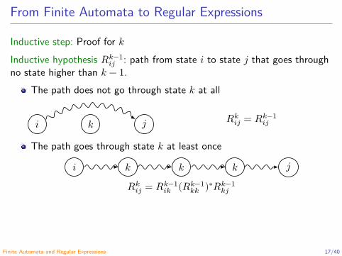
From Finite Automata to Regular Expressions
Inductive step: Proof for 𝑘Inductive hypothesis 𝑅𝑘−1
𝑖𝑗 : path from state 𝑖 to state 𝑗 that goes throughno state higher than 𝑘 − 1.
The path does not go through state 𝑘 at all
𝑖 𝑘 𝑗 𝑅𝑘𝑖𝑗 = 𝑅𝑘−1
𝑖𝑗
The path goes through state 𝑘 at least once
𝑖 𝑘 𝑘 𝑘 𝑗𝑅𝑘
𝑖𝑗 = 𝑅𝑘−1𝑖𝑘 (𝑅𝑘−1
𝑘𝑘 )∗𝑅𝑘−1𝑘𝑗
From the previous cases:
𝑅𝑘𝑖𝑗 = 𝑅𝑘−1
𝑖𝑗 + 𝑅𝑘−1𝑖𝑘 (𝑅𝑘−1
𝑘𝑘 )∗𝑅𝑘−1𝑘𝑗
Finite Automata and Regular Expressions 17/40
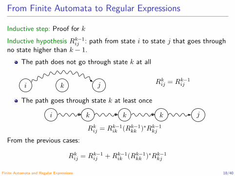
From Finite Automata to Regular Expressions
Inductive step: Proof for 𝑘Inductive hypothesis 𝑅𝑘−1
𝑖𝑗 : path from state 𝑖 to state 𝑗 that goes throughno state higher than 𝑘 − 1.
The path does not go through state 𝑘 at all
𝑖 𝑘 𝑗 𝑅𝑘𝑖𝑗 = 𝑅𝑘−1
𝑖𝑗
The path goes through state 𝑘 at least once
𝑖 𝑘 𝑘 𝑘 𝑗𝑅𝑘
𝑖𝑗 = 𝑅𝑘−1𝑖𝑘 (𝑅𝑘−1
𝑘𝑘 )∗𝑅𝑘−1𝑘𝑗
From the previous cases:
𝑅𝑘𝑖𝑗 = 𝑅𝑘−1
𝑖𝑗 + 𝑅𝑘−1𝑖𝑘 (𝑅𝑘−1
𝑘𝑘 )∗𝑅𝑘−1𝑘𝑗
Finite Automata and Regular Expressions 18/40

From Finite Automata to Regular Expressions
Given that the states of 𝐷 are {1, 2, … , 𝑛} with 1 the start state, then
𝐿(𝐷) = 𝐿(𝑅𝑛1𝑓1
+ ⋯ + 𝑅𝑛1𝑓𝑚
) with 𝑓𝑖 ∈ 𝐹.
Finite Automata and Regular Expressions 19/40

From Finite Automata to Regular Expressions
ExampleTo convert the DFA 𝐷 to a regular expression.
1start 2
10 0, 1
𝐿(𝐷) = {𝑤 ∈ {0, 1}∗ ∣ 𝑤 has at least one 0}.
Finite Automata and Regular Expressions 20/40

From Finite Automata to Regular Expressions
Example (cont.)
1start 2
10 0, 1
𝑅0𝑖𝑗
𝑅0𝑖𝑗 Regexp
𝑅011 𝜀 + 1
𝑅012 0
𝑅021 ∅
𝑅022 𝜀 + 0 + 1
Finite Automata and Regular Expressions 21/40

From Finite Automata to Regular Expressions
Example (cont.)𝑅1
𝑖𝑗 = 𝑅0𝑖𝑗 + 𝑅0
𝑖1(𝑅011)∗𝑅0
1𝑗
𝑅0𝑖𝑗 Regexp
𝑅011 𝜀 + 1
𝑅012 0
𝑅021 ∅
𝑅022 𝜀 + 0 + 1
𝑅1𝑖𝑗 Regexp
𝑅111 (𝜀 + 1) + (𝜀 + 1)(𝜀 + 1)∗(𝜀 + 1)
𝑅112 0 + (𝜀 + 1)(𝜀 + 1)∗0
𝑅121 ∅ + ∅(𝜀 + 1)∗(𝜀 + 1)
𝑅122 𝜀 + 0 + 1 + ∅(𝜀 + 1)∗0
Finite Automata and Regular Expressions 22/40
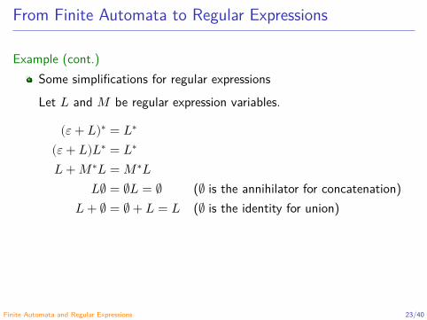
From Finite Automata to Regular Expressions
Example (cont.)Some simplifications for regular expressionsLet 𝐿 and 𝑀 be regular expression variables.
(𝜀 + 𝐿)∗ = 𝐿∗
(𝜀 + 𝐿)𝐿∗ = 𝐿∗
𝐿 + 𝑀∗𝐿 = 𝑀∗𝐿𝐿∅ = ∅𝐿 = ∅ (∅ is the annihilator for concatenation)
𝐿 + ∅ = ∅ + 𝐿 = 𝐿 (∅ is the identity for union)
Finite Automata and Regular Expressions 23/40
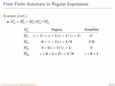
From Finite Automata to Regular Expressions
Example (cont.)𝑅1
𝑖𝑗 = 𝑅0𝑖𝑗 + 𝑅0
𝑖1(𝑅011)∗𝑅0
1𝑗
𝑅1𝑖𝑗 Regexp Simplified
𝑅111 (𝜀 + 1) + (𝜀 + 1)(𝜀 + 1)∗(𝜀 + 1) 1∗
𝑅112 0 + (𝜀 + 1)(𝜀 + 1)∗0 1∗0
𝑅121 ∅ + ∅(𝜀 + 1)∗(𝜀 + 1) ∅
𝑅122 𝜀 + 0 + 1 + ∅(𝜀 + 1)∗0 𝜀 + 0 + 1
Finite Automata and Regular Expressions 24/40

From Finite Automata to Regular Expressions
Example (cont.)𝑅2
𝑖𝑗 = 𝑅1𝑖𝑗 + 𝑅1
𝑖2(𝑅122)∗𝑅1
2𝑗
𝑅1𝑖𝑗 Regexp
𝑅111 1∗
𝑅112 1∗0
𝑅121 ∅
𝑅122 𝜀 + 0 + 1
𝑅2𝑖𝑗 Regexp
𝑅211 1∗ + 1∗0(𝜀 + 0 + 1)∗∅
𝑅212 1∗0 + 1∗0(𝜀 + 0 + 1)∗(𝜀 + 0 + 1)
𝑅221 ∅ + (𝜀 + 0 + 1)(𝜀 + 0 + 1)∗∅
𝑅222 𝜀 + 0 + 1 + (𝜀 + 0 + 1)(𝜀 + 0 + 1)∗(𝜀 + 0 + 1)
Finite Automata and Regular Expressions 25/40

From Finite Automata to Regular Expressions
Example (cont.)𝑅2
𝑖𝑗 = 𝑅1𝑖𝑗 + 𝑅1
𝑖2(𝑅122)∗𝑅1
2𝑗
𝑅2𝑖𝑗 Regexp Simplified
𝑅211 1∗ + 1∗0(𝜀 + 0 + 1)∗∅ 1∗
𝑅212 1∗0 + 1∗0(𝜀 + 0 + 1)∗(𝜀 + 0 + 1) 1∗0(0 + 1)∗
𝑅221 ∅ + (𝜀 + 0 + 1)(𝜀 + 0 + 1)∗∅ ∅
𝑅222 𝜀 + 0 + 1 + (𝜀 + 0 + 1)(𝜀 + 0 + 1)∗(𝜀 + 0 + 1) (0 + 1)∗
Finite Automata and Regular Expressions 26/40

From Finite Automata to Regular Expressions
Example (cont.)The regular expression equivalent to the automaton 𝐷 is
𝑅212 = 1∗0(0 + 1)∗.
Finite Automata and Regular Expressions 27/40
From Regular Expressions to Finite Automata
Theorem (3.7)
Every language defined by a regular expression is also defined by a finiteautomaton.
Inductive proofFor each regular expression 𝑅 we construct an 𝜀-NFA 𝐸 such that 𝐿(𝑅) =𝐿(𝐸) with:
1. exactly one accepting state,2. no arcs into the initial state and3. no arcs out of the accepting state.
Finite Automata and Regular Expressions 28/40
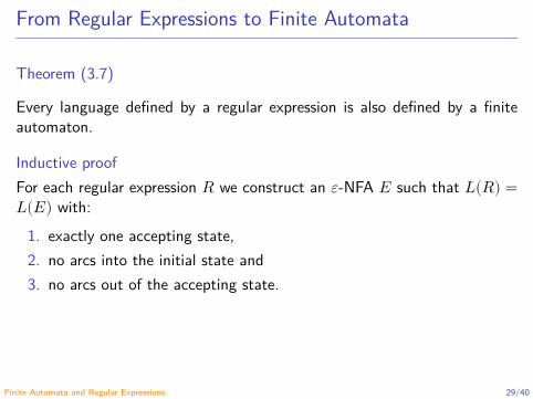
From Regular Expressions to Finite Automata
Theorem (3.7)
Every language defined by a regular expression is also defined by a finiteautomaton.
Inductive proofFor each regular expression 𝑅 we construct an 𝜀-NFA 𝐸 such that 𝐿(𝑅) =𝐿(𝐸) with:
1. exactly one accepting state,2. no arcs into the initial state and3. no arcs out of the accepting state.
Finite Automata and Regular Expressions 29/40

From Regular Expressions to Finite Automata
Basis step: Automata for 𝜀 (a), ∅ (b) and a (c).†
From regex’s to ε-NFA’s
Theorem 3.7: For every regex R we can con-
struct and ε-NFA A, s.t. L(A) = L(R).
Proof: By structural induction:
Basis: Automata for ε, ∅, and a.
ε
a
(a)
(b)
(c)
73
†Figure from Hopcroft, Motwani and Ullman (2007, Fig. 3.16).Finite Automata and Regular Expressions 30/40
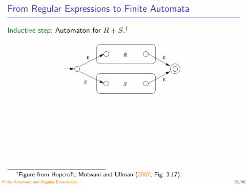
From Regular Expressions to Finite Automata
Inductive step: Automaton for 𝑅 + 𝑆.†���� FINITE AUTOMATA AND REGULAR EXPRESSIONS ���
(a)
(b)
(c)
R
S
R S
R
ε ε
εε
ε
ε
ε
ε ε
Figure ����� The inductive step in the regularexpressionto�NFA construction
automaton of Fig� �����c�� That automaton allows us to go either�
�a� Directly from the start state to the accepting state along a pathlabeled �� That path lets us accept �� which is in L�R�� no matterwhat expression R is�
�b� To the start state of the automaton for R� through that automatonone or more times� and then to the accepting state� This set of pathsallows us to accept strings in L�R�� L�R�L�R�� L�R�L�R�L�R�� andso on� thus covering all strings in L�R�� except perhaps �� which wascovered by the direct arc to the accepting state mentioned in ��a��
�� The expression is �R� for some smaller expression R� The automatonfor R also serves as the automaton for �R�� since the parentheses do notchange the language de ned by the expression�
It is a simple observation that the constructed automata satisfy the three conditions given in the inductive hypothesis � one accepting state� with no arcsinto the initial state or out of the accepting state� �
†Figure from Hopcroft, Motwani and Ullman (2007, Fig. 3.17).Finite Automata and Regular Expressions 31/40

From Regular Expressions to Finite Automata
Inductive step: Automaton for 𝑅𝑆.†
���� FINITE AUTOMATA AND REGULAR EXPRESSIONS ���
(a)
(b)
(c)
R
S
R S
R
ε ε
εε
ε
ε
ε
ε ε
Figure ����� The inductive step in the regularexpressionto�NFA construction
automaton of Fig� �����c�� That automaton allows us to go either�
�a� Directly from the start state to the accepting state along a pathlabeled �� That path lets us accept �� which is in L�R�� no matterwhat expression R is�
�b� To the start state of the automaton for R� through that automatonone or more times� and then to the accepting state� This set of pathsallows us to accept strings in L�R�� L�R�L�R�� L�R�L�R�L�R�� andso on� thus covering all strings in L�R�� except perhaps �� which wascovered by the direct arc to the accepting state mentioned in ��a��
�� The expression is �R� for some smaller expression R� The automatonfor R also serves as the automaton for �R�� since the parentheses do notchange the language de ned by the expression�
It is a simple observation that the constructed automata satisfy the three conditions given in the inductive hypothesis � one accepting state� with no arcsinto the initial state or out of the accepting state� �
†Figure from Hopcroft, Motwani and Ullman (2007, Fig. 3.17).Finite Automata and Regular Expressions 32/40

From Regular Expressions to Finite Automata
Inductive step: Automaton for 𝑅∗.†
���� FINITE AUTOMATA AND REGULAR EXPRESSIONS ���
(a)
(b)
(c)
R
S
R S
R
ε ε
εε
ε
ε
ε
ε ε
Figure ����� The inductive step in the regularexpressionto�NFA construction
automaton of Fig� �����c�� That automaton allows us to go either�
�a� Directly from the start state to the accepting state along a pathlabeled �� That path lets us accept �� which is in L�R�� no matterwhat expression R is�
�b� To the start state of the automaton for R� through that automatonone or more times� and then to the accepting state� This set of pathsallows us to accept strings in L�R�� L�R�L�R�� L�R�L�R�L�R�� andso on� thus covering all strings in L�R�� except perhaps �� which wascovered by the direct arc to the accepting state mentioned in ��a��
�� The expression is �R� for some smaller expression R� The automatonfor R also serves as the automaton for �R�� since the parentheses do notchange the language de ned by the expression�
It is a simple observation that the constructed automata satisfy the three conditions given in the inductive hypothesis � one accepting state� with no arcsinto the initial state or out of the accepting state� �
†Figure from Hopcroft, Motwani and Ullman (2007, Fig. 3.17).Finite Automata and Regular Expressions 33/40

From Regular Expressions to Finite Automata
ExampleConvert the regular expression 𝑅 = (0 + 1)∗1(0 + 1) to an 𝜀-NFA 𝐸 such𝐿(𝑅) = 𝐿(𝐸).
1. 𝜀-NFA for 0 + 1:
start𝜀
𝜀
0 𝜀
1𝜀
Finite Automata and Regular Expressions 34/40
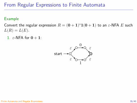
From Regular Expressions to Finite Automata
ExampleConvert the regular expression 𝑅 = (0 + 1)∗1(0 + 1) to an 𝜀-NFA 𝐸 such𝐿(𝑅) = 𝐿(𝐸).
1. 𝜀-NFA for 0 + 1:
start𝜀
𝜀
0 𝜀
1𝜀
Finite Automata and Regular Expressions 35/40
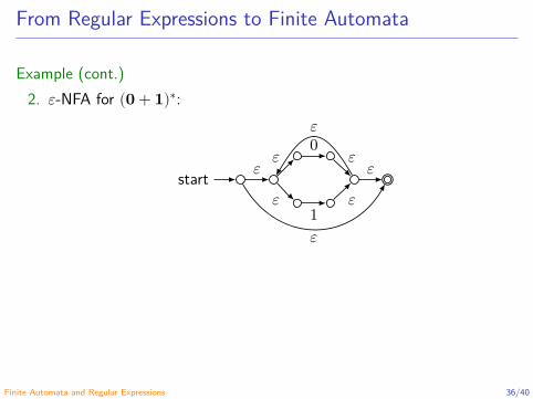
From Regular Expressions to Finite Automata
Example (cont.)2. 𝜀-NFA for (0 + 1)∗:
start 𝜀 𝜀
𝜀
0 𝜀
1𝜀
𝜀
𝜀
𝜀
Finite Automata and Regular Expressions 36/40

From Regular Expressions to Finite Automata
Example (cont.)3. 𝜀-NFA for (0 + 1)∗1:
start 𝜀 𝜀
𝜀
0 𝜀
1𝜀
𝜀
𝜀
𝜀
𝜀 1
Finite Automata and Regular Expressions 37/40

From Regular Expressions to Finite Automata
Example (cont.)4. 𝜀-NFA for (0 + 1)∗1(0 + 1):
start 𝜀 𝜀
𝜀
0 𝜀
1𝜀
𝜀
𝜀
𝜀
𝜀 1 𝜀 𝜀
𝜀
0 𝜀
1𝜀
Finite Automata and Regular Expressions 38/40
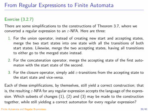
From Regular Expressions to Finite Automata
Exercise (3.2.7)There are some simplifications to the constructions of Theorem 3.7, where weconverted a regular expression to an 𝜀-NFA. Here are three:
1. For the union operator, instead of creating new start and accepting states,merge the two start states into one state with all the transitions of bothstart states. Likewise, merge the two accepting states, having all transitionsto either go to the merged state instead.
2. For the concatenation operator, merge the accepting state of the first auto-maton with the start state of the second.
3. For the closure operator, simply add 𝜀-transitions from the accepting state tothe start state and vice-versa.
Each of these simplifications, by themselves, still yield a correct construction; thatis, the resulting 𝜀-NFA for any regular expression accepts the language of the expres-sion. Which subsets of changes (1), (2) and (3) may be made to the constructiontogether, while still yielding a correct automaton for every regular expression?
Finite Automata and Regular Expressions 39/40

References
Hopcroft, J. E., Motwani, R. and Ullman, J. D. (2007). Introduction toAutomata theory, Languages, and Computation. 3rd ed. Pearson Education(cit. on pp. 4, 5, 30–33).
Finite Automata and Regular Expressions 40/40

Automata and Formal Languages - CM0081Algebraic Laws for Regular Expressions
Andrés Sicard-Ramírez
Universidad EAFIT
Semester 2018-1
Algebraic Laws for Regular Expressions
DefinitionTwo regular expressions with variables are equivalent if whatever languageswe substitute for the variables, the results of the two expressions are thesame language.
NotationLet 𝐿, 𝑀 and 𝑁 be regular expression variables.
Sugar syntax
𝐿+ def= 𝐿𝐿∗,𝐿? def= 𝜀 + 𝐿.
Algebraic Laws for Regular Expressions 2/33
Algebraic Laws for Regular Expressions
DefinitionTwo regular expressions with variables are equivalent if whatever languageswe substitute for the variables, the results of the two expressions are thesame language.
NotationLet 𝐿, 𝑀 and 𝑁 be regular expression variables.
Sugar syntax
𝐿+ def= 𝐿𝐿∗,𝐿? def= 𝜀 + 𝐿.
Algebraic Laws for Regular Expressions 3/33

Algebraic Laws for Regular Expressions
DefinitionTwo regular expressions with variables are equivalent if whatever languageswe substitute for the variables, the results of the two expressions are thesame language.
NotationLet 𝐿, 𝑀 and 𝑁 be regular expression variables.
Sugar syntax
𝐿+ def= 𝐿𝐿∗,𝐿? def= 𝜀 + 𝐿.
Algebraic Laws for Regular Expressions 4/33
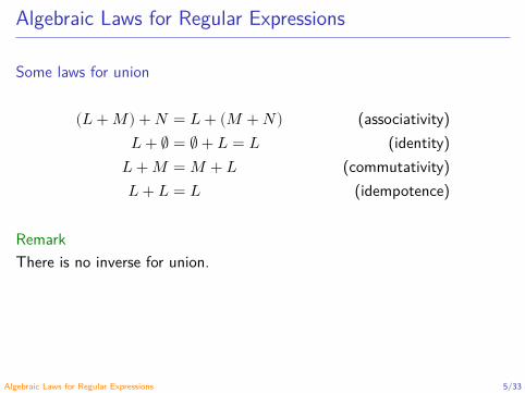
Algebraic Laws for Regular Expressions
Some laws for union
(𝐿 +𝑀) +𝑁 = 𝐿+ (𝑀 +𝑁) (associativity)𝐿 + ∅ = ∅ + 𝐿 = 𝐿 (identity)
𝐿 +𝑀 = 𝑀 +𝐿 (commutativity)𝐿 + 𝐿 = 𝐿 (idempotence)
RemarkThere is no inverse for union.
Algebraic Laws for Regular Expressions 5/33
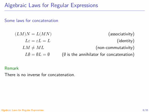
Algebraic Laws for Regular Expressions
Some laws for concatenation
(𝐿𝑀)𝑁 = 𝐿(𝑀𝑁) (associativity)𝐿𝜀 = 𝜀𝐿 = 𝐿 (identity)
𝐿𝑀 ≠ 𝑀𝐿 (non-commutativity)𝐿∅ = ∅𝐿 = ∅ (∅ is the annihilator for concatenation)
RemarkThere is no inverse for concatenation.
Algebraic Laws for Regular Expressions 6/33
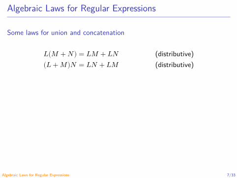
Algebraic Laws for Regular Expressions
Some laws for union and concatenation
𝐿(𝑀 +𝑁) = 𝐿𝑀 +𝐿𝑁 (distributive)(𝐿 +𝑀)𝑁 = 𝐿𝑁 + 𝐿𝑀 (distributive)
Algebraic Laws for Regular Expressions 7/33

Algebraic Laws for Regular Expressions
Some laws for closure
(𝐿∗)∗ = 𝐿∗ (idempotence)∅∗ = 𝜀𝜀∗ = 𝜀
(𝜀 + 𝐿)∗ = 𝐿∗
𝐿∗ = 𝐿+ + 𝜀
Algebraic Laws for Regular Expressions 8/33

Simplification of Regular Expressions
Example
0 + (𝜀 + 1)(𝜀 + 1)∗0 = 0 + (𝜀 + 1)1∗0 ((𝜀 + 𝐿)∗ = 𝐿∗)= 0 + (𝜀1∗ + 11∗)0 (distributive)= 0 + (1∗ + 11∗)0 (identity)= 0 + (1∗ + 1+)0 (def. 𝐿+)= 0 + 1∗0 (equivalence)= 1∗0 (equivalence)
Algebraic Laws for Regular Expressions 9/33

Discovering Laws for Regular Expressions
MethodLet 𝐸 and 𝐹 be two regular expressions with the same set of variables{𝐿1,… , 𝐿𝑛}.To test if 𝐸 = 𝐹 :
1. Convert 𝐸 and 𝐹 to concrete regular expressions 𝐶 and 𝐷, replacingeach 𝐿𝑖 by a different symbol a𝑖, for 𝑖 = 1, 2,… , 𝑛.
2. Test whether 𝐿(𝐶) = 𝐿(𝐷). If so, then 𝐸 = 𝐹 , and if not 𝐸 ≠ 𝐹 .
ObservationWe are proving by example!
Algebraic Laws for Regular Expressions 10/33
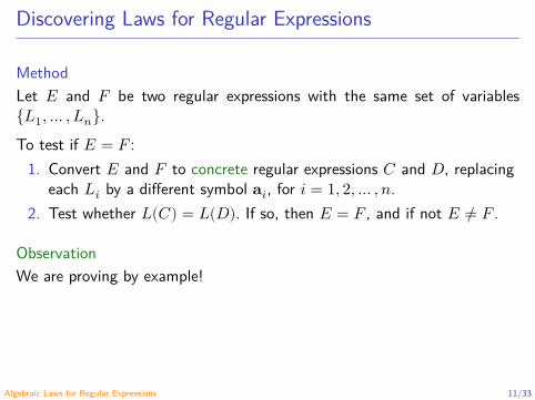
Discovering Laws for Regular Expressions
MethodLet 𝐸 and 𝐹 be two regular expressions with the same set of variables{𝐿1,… , 𝐿𝑛}.To test if 𝐸 = 𝐹 :
1. Convert 𝐸 and 𝐹 to concrete regular expressions 𝐶 and 𝐷, replacingeach 𝐿𝑖 by a different symbol a𝑖, for 𝑖 = 1, 2,… , 𝑛.
2. Test whether 𝐿(𝐶) = 𝐿(𝐷). If so, then 𝐸 = 𝐹 , and if not 𝐸 ≠ 𝐹 .
ObservationWe are proving by example!
Algebraic Laws for Regular Expressions 11/33

Discovering Laws for Regular Expressions
ExampleProve or disprove that 𝐿∗ = 𝐿∗𝐿∗.
1. We replace the variable 𝐿 by the concrete regular expression a.2. a∗ ≟ a∗a∗.3. Because 𝐿(a∗) = 𝐿(a∗a∗), we conclude that 𝐿∗ = 𝐿∗𝐿∗.
Algebraic Laws for Regular Expressions 12/33
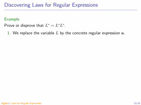
Discovering Laws for Regular Expressions
ExampleProve or disprove that 𝐿∗ = 𝐿∗𝐿∗.
1. We replace the variable 𝐿 by the concrete regular expression a.
2. a∗ ≟ a∗a∗.3. Because 𝐿(a∗) = 𝐿(a∗a∗), we conclude that 𝐿∗ = 𝐿∗𝐿∗.
Algebraic Laws for Regular Expressions 13/33
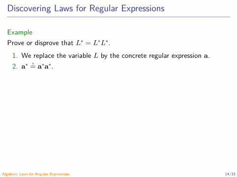
Discovering Laws for Regular Expressions
ExampleProve or disprove that 𝐿∗ = 𝐿∗𝐿∗.
1. We replace the variable 𝐿 by the concrete regular expression a.2. a∗ ≟ a∗a∗.
3. Because 𝐿(a∗) = 𝐿(a∗a∗), we conclude that 𝐿∗ = 𝐿∗𝐿∗.
Algebraic Laws for Regular Expressions 14/33
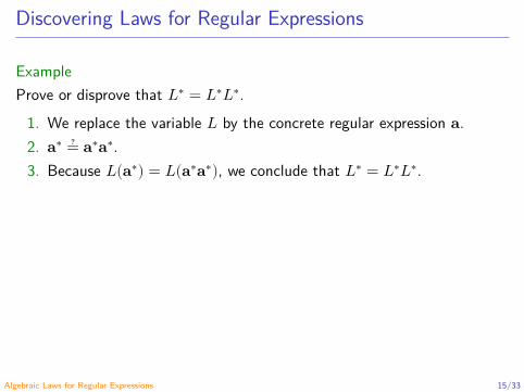
Discovering Laws for Regular Expressions
ExampleProve or disprove that 𝐿∗ = 𝐿∗𝐿∗.
1. We replace the variable 𝐿 by the concrete regular expression a.2. a∗ ≟ a∗a∗.3. Because 𝐿(a∗) = 𝐿(a∗a∗), we conclude that 𝐿∗ = 𝐿∗𝐿∗.
Algebraic Laws for Regular Expressions 15/33

Discovering Laws for Regular Expressions
ExampleProve or disprove that 𝐿 +𝑀𝐿 = (𝐿 +𝑀)𝐿.
1. We replace the variables 𝐿 and 𝑀 by the concrete regularexpressions a and b respectively.
2. a + ba ≟ (a + b)a.3. 𝑎𝑎 ∉ 𝐿(a + ba) and 𝑎𝑎 ∈ 𝐿((a + b)a)
⇒ 𝐿(a + ba) ≠ 𝐿((a + b)a)⇒ 𝐿 +𝑀𝐿 ≠ (𝐿 +𝑀)𝐿
Algebraic Laws for Regular Expressions 16/33
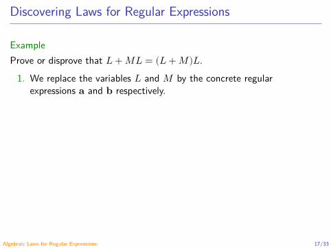
Discovering Laws for Regular Expressions
ExampleProve or disprove that 𝐿 +𝑀𝐿 = (𝐿 +𝑀)𝐿.
1. We replace the variables 𝐿 and 𝑀 by the concrete regularexpressions a and b respectively.
2. a + ba ≟ (a + b)a.3. 𝑎𝑎 ∉ 𝐿(a + ba) and 𝑎𝑎 ∈ 𝐿((a + b)a)
⇒ 𝐿(a + ba) ≠ 𝐿((a + b)a)⇒ 𝐿 +𝑀𝐿 ≠ (𝐿 +𝑀)𝐿
Algebraic Laws for Regular Expressions 17/33
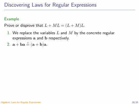
Discovering Laws for Regular Expressions
ExampleProve or disprove that 𝐿 +𝑀𝐿 = (𝐿 +𝑀)𝐿.
1. We replace the variables 𝐿 and 𝑀 by the concrete regularexpressions a and b respectively.
2. a + ba ≟ (a + b)a.
3. 𝑎𝑎 ∉ 𝐿(a + ba) and 𝑎𝑎 ∈ 𝐿((a + b)a)⇒ 𝐿(a + ba) ≠ 𝐿((a + b)a)⇒ 𝐿 +𝑀𝐿 ≠ (𝐿 +𝑀)𝐿
Algebraic Laws for Regular Expressions 18/33

Discovering Laws for Regular Expressions
ExampleProve or disprove that 𝐿 +𝑀𝐿 = (𝐿 +𝑀)𝐿.
1. We replace the variables 𝐿 and 𝑀 by the concrete regularexpressions a and b respectively.
2. a + ba ≟ (a + b)a.3. 𝑎𝑎 ∉ 𝐿(a + ba) and 𝑎𝑎 ∈ 𝐿((a + b)a)
⇒ 𝐿(a + ba) ≠ 𝐿((a + b)a)⇒ 𝐿 +𝑀𝐿 ≠ (𝐿 +𝑀)𝐿
Algebraic Laws for Regular Expressions 19/33
Discovering Laws for Regular Expressions
Example (Exercise 3.4.2.d)Prove or disprove that (𝐿 +𝑀)∗𝑀 = (𝐿∗𝑀)∗.
1. We replace the variables 𝐿 and 𝑀 by the concrete regularexpressions a and b respectively.
2. (a + b)∗b ≟ (a∗b)∗.3. Since 𝜀 ∉ (a + b)∗b and 𝜀 ∈ (a∗b)∗
⇒ (𝐿 +𝑀)∗𝑀 ≠ (𝐿∗𝑀)∗
Algebraic Laws for Regular Expressions 20/33
Discovering Laws for Regular Expressions
Example (Exercise 3.4.2.d)Prove or disprove that (𝐿 +𝑀)∗𝑀 = (𝐿∗𝑀)∗.
1. We replace the variables 𝐿 and 𝑀 by the concrete regularexpressions a and b respectively.
2. (a + b)∗b ≟ (a∗b)∗.3. Since 𝜀 ∉ (a + b)∗b and 𝜀 ∈ (a∗b)∗
⇒ (𝐿 +𝑀)∗𝑀 ≠ (𝐿∗𝑀)∗
Algebraic Laws for Regular Expressions 21/33
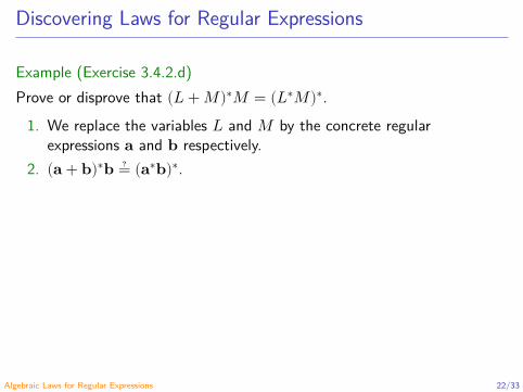
Discovering Laws for Regular Expressions
Example (Exercise 3.4.2.d)Prove or disprove that (𝐿 +𝑀)∗𝑀 = (𝐿∗𝑀)∗.
1. We replace the variables 𝐿 and 𝑀 by the concrete regularexpressions a and b respectively.
2. (a + b)∗b ≟ (a∗b)∗.
3. Since 𝜀 ∉ (a + b)∗b and 𝜀 ∈ (a∗b)∗
⇒ (𝐿 +𝑀)∗𝑀 ≠ (𝐿∗𝑀)∗
Algebraic Laws for Regular Expressions 22/33
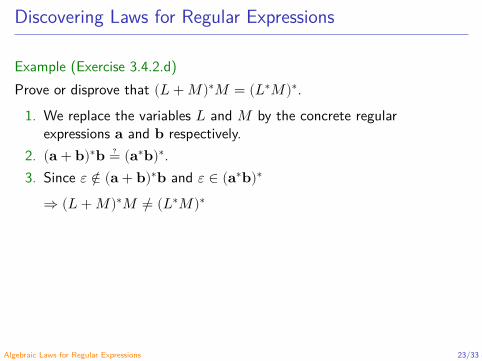
Discovering Laws for Regular Expressions
Example (Exercise 3.4.2.d)Prove or disprove that (𝐿 +𝑀)∗𝑀 = (𝐿∗𝑀)∗.
1. We replace the variables 𝐿 and 𝑀 by the concrete regularexpressions a and b respectively.
2. (a + b)∗b ≟ (a∗b)∗.3. Since 𝜀 ∉ (a + b)∗b and 𝜀 ∈ (a∗b)∗
⇒ (𝐿 +𝑀)∗𝑀 ≠ (𝐿∗𝑀)∗
Algebraic Laws for Regular Expressions 23/33
Discovering Laws for Regular Expressions
Example (counter-example)Extensions of the previous test beyond regular expressions may fail.
1. Add ∩ to the regular expression operators.2. Test if 𝐿 ∩𝑀 ∩𝑁 = 𝐿 ∩𝑀 .3. From 𝐿 = a, 𝑀 = b and 𝑁 = c and since
{𝑎} ∩ {𝑏} ∩ {𝑐} = ∅ = {𝑎} ∩ {𝑏},
we should conclude that the “property” is true.4. But, the “property” is false. For example, if 𝐿 = 𝑀 = a and 𝑁 = ∅
then𝐿 ∩𝑀 ∩𝑁 ≠ 𝐿 ∩𝑀.
5. Therefore, the test is not valid!
Algebraic Laws for Regular Expressions 24/33
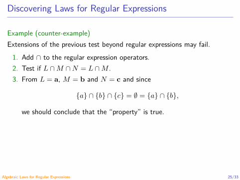
Discovering Laws for Regular Expressions
Example (counter-example)Extensions of the previous test beyond regular expressions may fail.
1. Add ∩ to the regular expression operators.2. Test if 𝐿 ∩𝑀 ∩𝑁 = 𝐿 ∩𝑀 .3. From 𝐿 = a, 𝑀 = b and 𝑁 = c and since
{𝑎} ∩ {𝑏} ∩ {𝑐} = ∅ = {𝑎} ∩ {𝑏},
we should conclude that the “property” is true.
4. But, the “property” is false. For example, if 𝐿 = 𝑀 = a and 𝑁 = ∅then
𝐿 ∩𝑀 ∩𝑁 ≠ 𝐿 ∩𝑀.5. Therefore, the test is not valid!
Algebraic Laws for Regular Expressions 25/33

Discovering Laws for Regular Expressions
Example (counter-example)Extensions of the previous test beyond regular expressions may fail.
1. Add ∩ to the regular expression operators.2. Test if 𝐿 ∩𝑀 ∩𝑁 = 𝐿 ∩𝑀 .3. From 𝐿 = a, 𝑀 = b and 𝑁 = c and since
{𝑎} ∩ {𝑏} ∩ {𝑐} = ∅ = {𝑎} ∩ {𝑏},
we should conclude that the “property” is true.4. But, the “property” is false. For example, if 𝐿 = 𝑀 = a and 𝑁 = ∅
then𝐿 ∩𝑀 ∩𝑁 ≠ 𝐿 ∩𝑀.
5. Therefore, the test is not valid!
Algebraic Laws for Regular Expressions 26/33

Derivative of a Regular Expression
From (Brzozowski 1964).
DefinitionLet 𝐿 ⊆ Σ∗ be a language and 𝑎 ∈ Σ a symbol. We define the derivativeof 𝐿 by 𝑎, denoted by 𝑎\𝐿, by
𝑎\𝐿 = {𝑥 ∈ Σ∗ ∣ 𝑎𝑥 ∈ 𝐿}.
Examples
𝑎\{𝑎𝑏𝑎𝑏, 𝑎𝑏𝑏𝑎} = {𝑏𝑎𝑏, 𝑏𝑏𝑎},𝑎\𝐿(ab∗) = 𝐿(b∗),𝑏\𝐿(ab∗) = ∅.
Algebraic Laws for Regular Expressions 27/33

Derivative of a Regular Expression
From (Brzozowski 1964).
DefinitionLet 𝐿 ⊆ Σ∗ be a language and 𝑎 ∈ Σ a symbol. We define the derivativeof 𝐿 by 𝑎, denoted by 𝑎\𝐿, by
𝑎\𝐿 = {𝑥 ∈ Σ∗ ∣ 𝑎𝑥 ∈ 𝐿}.
Examples
𝑎\{𝑎𝑏𝑎𝑏, 𝑎𝑏𝑏𝑎} = {𝑏𝑎𝑏, 𝑏𝑏𝑎},𝑎\𝐿(ab∗) = 𝐿(b∗),𝑏\𝐿(ab∗) = ∅.
Algebraic Laws for Regular Expressions 28/33
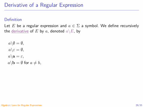
Derivative of a Regular Expression
DefinitionLet 𝐸 be a regular expression and 𝑎 ∈ Σ a symbol. We define recursivelythe derivative of 𝐸 by 𝑎, denoted 𝑎\𝐸, by
𝑎\∅ = ∅,𝑎\𝜀 = ∅,𝑎\a = 𝜀,𝑎\b = ∅ for 𝑎 ≠ 𝑏,
𝑎\(𝐸 + 𝐹) = 𝑎\𝐸 + 𝑎\𝐹 ,
𝑎\(𝐸𝐹) = {(𝑎\𝐸)𝐹 + 𝑎\𝐹 , if 𝜀 ∈ 𝐿(𝐸),(𝑎\𝐸)𝐹 , otherwise,
𝑎\(𝐸∗) = (𝑎\𝐸)𝐸∗.
Algebraic Laws for Regular Expressions 29/33
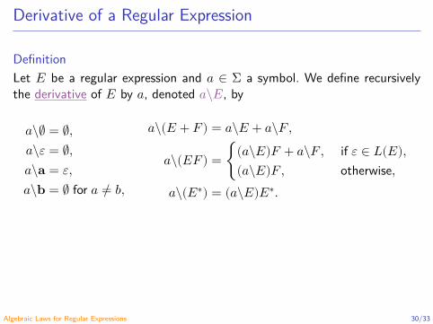
Derivative of a Regular Expression
DefinitionLet 𝐸 be a regular expression and 𝑎 ∈ Σ a symbol. We define recursivelythe derivative of 𝐸 by 𝑎, denoted 𝑎\𝐸, by
𝑎\∅ = ∅,𝑎\𝜀 = ∅,𝑎\a = 𝜀,𝑎\b = ∅ for 𝑎 ≠ 𝑏,
𝑎\(𝐸 + 𝐹) = 𝑎\𝐸 + 𝑎\𝐹 ,
𝑎\(𝐸𝐹) = {(𝑎\𝐸)𝐹 + 𝑎\𝐹 , if 𝜀 ∈ 𝐿(𝐸),(𝑎\𝐸)𝐹 , otherwise,
𝑎\(𝐸∗) = (𝑎\𝐸)𝐸∗.
Algebraic Laws for Regular Expressions 30/33
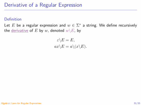
Derivative of a Regular Expression
DefinitionLet 𝐸 be a regular expression and 𝑤 ∈ Σ∗ a string. We define recursivelythe derivative of 𝐸 by 𝑤, denoted 𝑤\𝐸, by
𝜀\𝐸 = 𝐸,𝑎𝑥\𝐸 = 𝑎\(𝑥\𝐸).
Theorem (Brzozowski (1964), Theorem 4.2)
𝑤 ∈ 𝐿(𝐸) ⇔ 𝜀 ∈ 𝐿(𝑤\𝐸).
Algebraic Laws for Regular Expressions 31/33
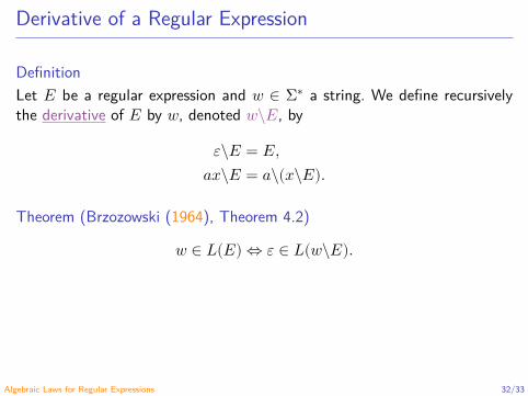
Derivative of a Regular Expression
DefinitionLet 𝐸 be a regular expression and 𝑤 ∈ Σ∗ a string. We define recursivelythe derivative of 𝐸 by 𝑤, denoted 𝑤\𝐸, by
𝜀\𝐸 = 𝐸,𝑎𝑥\𝐸 = 𝑎\(𝑥\𝐸).
Theorem (Brzozowski (1964), Theorem 4.2)
𝑤 ∈ 𝐿(𝐸) ⇔ 𝜀 ∈ 𝐿(𝑤\𝐸).
Algebraic Laws for Regular Expressions 32/33
References
Brzozowski, J. A. (1964). Derivates of Regular Expressions. Journal of theACM 11.4, pp. 481–494. doi: 10.1145/321239.321249 (cit. on pp. 27, 28,31, 32).
Algebraic Laws for Regular Expressions 33/33

Automata and Formal Languages - CM0081Proving Languages Not to Be Regular
Andrés Sicard-Ramírez
Universidad EAFIT
Semester 2018-1
Properties of Regular Languages
Proving languages not to be regularClosure propertiesDecision propertiesEquivalence and minimization of automata
Proving Languages Not to Be Regular 2/36
The Pumping Lemma
IntroductionIs 𝐿 = {0𝑚1𝑛 ∣ 𝑚, 𝑛 ≥ 0} a regular language?
Yes! 𝐿 = 𝐿(0∗1∗).Is 𝐿 = {0𝑚1𝑛 ∣ 𝑚, 𝑛 ≥ 1} a regular language?Yes! 𝐿 = 𝐿(0+1+).Is 𝐿 = {0𝑚1𝑛 ∣ 𝑚 ≥ 2, 𝑛 ≥ 4} a regular language?Yes! 𝐿 = 𝐿(000∗11111∗).Is 𝐿01 = {0𝑛1𝑛 ∣ 𝑛 ≥ 1} a regular language?No! Informal proof (whiteboard).
Proving Languages Not to Be Regular 3/36

The Pumping Lemma
IntroductionIs 𝐿 = {0𝑚1𝑛 ∣ 𝑚, 𝑛 ≥ 0} a regular language?Yes! 𝐿 = 𝐿(0∗1∗).
Is 𝐿 = {0𝑚1𝑛 ∣ 𝑚, 𝑛 ≥ 1} a regular language?Yes! 𝐿 = 𝐿(0+1+).Is 𝐿 = {0𝑚1𝑛 ∣ 𝑚 ≥ 2, 𝑛 ≥ 4} a regular language?Yes! 𝐿 = 𝐿(000∗11111∗).Is 𝐿01 = {0𝑛1𝑛 ∣ 𝑛 ≥ 1} a regular language?No! Informal proof (whiteboard).
Proving Languages Not to Be Regular 4/36
The Pumping Lemma
IntroductionIs 𝐿 = {0𝑚1𝑛 ∣ 𝑚, 𝑛 ≥ 0} a regular language?Yes! 𝐿 = 𝐿(0∗1∗).Is 𝐿 = {0𝑚1𝑛 ∣ 𝑚, 𝑛 ≥ 1} a regular language?
Yes! 𝐿 = 𝐿(0+1+).Is 𝐿 = {0𝑚1𝑛 ∣ 𝑚 ≥ 2, 𝑛 ≥ 4} a regular language?Yes! 𝐿 = 𝐿(000∗11111∗).Is 𝐿01 = {0𝑛1𝑛 ∣ 𝑛 ≥ 1} a regular language?No! Informal proof (whiteboard).
Proving Languages Not to Be Regular 5/36

The Pumping Lemma
IntroductionIs 𝐿 = {0𝑚1𝑛 ∣ 𝑚, 𝑛 ≥ 0} a regular language?Yes! 𝐿 = 𝐿(0∗1∗).Is 𝐿 = {0𝑚1𝑛 ∣ 𝑚, 𝑛 ≥ 1} a regular language?Yes! 𝐿 = 𝐿(0+1+).
Is 𝐿 = {0𝑚1𝑛 ∣ 𝑚 ≥ 2, 𝑛 ≥ 4} a regular language?Yes! 𝐿 = 𝐿(000∗11111∗).Is 𝐿01 = {0𝑛1𝑛 ∣ 𝑛 ≥ 1} a regular language?No! Informal proof (whiteboard).
Proving Languages Not to Be Regular 6/36

The Pumping Lemma
IntroductionIs 𝐿 = {0𝑚1𝑛 ∣ 𝑚, 𝑛 ≥ 0} a regular language?Yes! 𝐿 = 𝐿(0∗1∗).Is 𝐿 = {0𝑚1𝑛 ∣ 𝑚, 𝑛 ≥ 1} a regular language?Yes! 𝐿 = 𝐿(0+1+).Is 𝐿 = {0𝑚1𝑛 ∣ 𝑚 ≥ 2, 𝑛 ≥ 4} a regular language?
Yes! 𝐿 = 𝐿(000∗11111∗).Is 𝐿01 = {0𝑛1𝑛 ∣ 𝑛 ≥ 1} a regular language?No! Informal proof (whiteboard).
Proving Languages Not to Be Regular 7/36
The Pumping Lemma
IntroductionIs 𝐿 = {0𝑚1𝑛 ∣ 𝑚, 𝑛 ≥ 0} a regular language?Yes! 𝐿 = 𝐿(0∗1∗).Is 𝐿 = {0𝑚1𝑛 ∣ 𝑚, 𝑛 ≥ 1} a regular language?Yes! 𝐿 = 𝐿(0+1+).Is 𝐿 = {0𝑚1𝑛 ∣ 𝑚 ≥ 2, 𝑛 ≥ 4} a regular language?Yes! 𝐿 = 𝐿(000∗11111∗).
Is 𝐿01 = {0𝑛1𝑛 ∣ 𝑛 ≥ 1} a regular language?No! Informal proof (whiteboard).
Proving Languages Not to Be Regular 8/36

The Pumping Lemma
IntroductionIs 𝐿 = {0𝑚1𝑛 ∣ 𝑚, 𝑛 ≥ 0} a regular language?Yes! 𝐿 = 𝐿(0∗1∗).Is 𝐿 = {0𝑚1𝑛 ∣ 𝑚, 𝑛 ≥ 1} a regular language?Yes! 𝐿 = 𝐿(0+1+).Is 𝐿 = {0𝑚1𝑛 ∣ 𝑚 ≥ 2, 𝑛 ≥ 4} a regular language?Yes! 𝐿 = 𝐿(000∗11111∗).Is 𝐿01 = {0𝑛1𝑛 ∣ 𝑛 ≥ 1} a regular language?
No! Informal proof (whiteboard).
Proving Languages Not to Be Regular 9/36

The Pumping Lemma
IntroductionIs 𝐿 = {0𝑚1𝑛 ∣ 𝑚, 𝑛 ≥ 0} a regular language?Yes! 𝐿 = 𝐿(0∗1∗).Is 𝐿 = {0𝑚1𝑛 ∣ 𝑚, 𝑛 ≥ 1} a regular language?Yes! 𝐿 = 𝐿(0+1+).Is 𝐿 = {0𝑚1𝑛 ∣ 𝑚 ≥ 2, 𝑛 ≥ 4} a regular language?Yes! 𝐿 = 𝐿(000∗11111∗).Is 𝐿01 = {0𝑛1𝑛 ∣ 𝑛 ≥ 1} a regular language?No! Informal proof (whiteboard).
Proving Languages Not to Be Regular 10/36
The Pumping Lemma
Theorem (Pumping Lemma for regular languages, 4.1)Let 𝐿 be a regular language, then
(∃𝑛 ∈ ℤ+)(∀𝑤 ∈ 𝐿) (|𝑤| ≥ 𝑛 ⇒ (∃𝑥 𝑦 𝑧) 𝑤 = 𝑥𝑦𝑧)
such that1. 𝑦 ≠ 𝜀,2. |𝑥𝑦| ≤ 𝑛 and3. (∀𝑘 ≥ 0) 𝑥𝑦𝑘𝑧 ∈ 𝐿.
Proving Languages Not to Be Regular 11/36
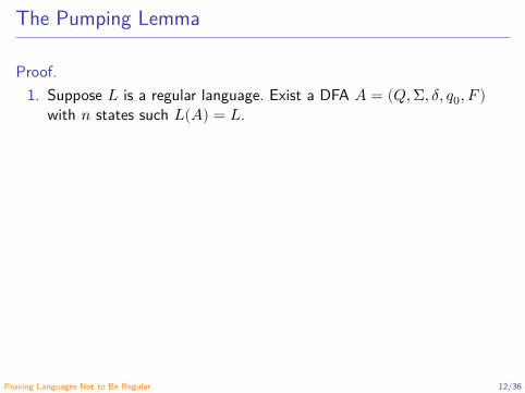
The Pumping Lemma
Proof.1. Suppose 𝐿 is a regular language. Exist a DFA 𝐴 = (𝑄, Σ, 𝛿, 𝑞0, 𝐹 )
with 𝑛 states such 𝐿(𝐴) = 𝐿.
2. Let 𝑤 = 𝑎1 ⋯ 𝑎𝑚 ∈ 𝐿, 𝑚 ≥ 𝑛 and 𝑞𝑖 = 𝛿(𝑞0, 𝑎1 ⋯ 𝑎𝑖).3. By the pigeonhole principle, exists 𝑖 and 𝑗, with 0 ≤ 𝑖 < 𝑗 ≤ 𝑛 such
𝑞𝑖 = 𝑞𝑗.4. Let 𝑤 = 𝑥𝑦𝑧 where
𝑞0start 𝑞𝑖𝑥 = 𝑎1 ⋯ 𝑎𝑖
𝑦 = 𝑎𝑖+1 ⋯ 𝑎𝑗
𝑧 = 𝑎𝑗+1 ⋯ 𝑎𝑚
5. Then (∀𝑘 ≥ 0) 𝑥𝑦𝑘𝑧 ∈ 𝐿.
Proving Languages Not to Be Regular 12/36

The Pumping Lemma
Proof.1. Suppose 𝐿 is a regular language. Exist a DFA 𝐴 = (𝑄, Σ, 𝛿, 𝑞0, 𝐹 )
with 𝑛 states such 𝐿(𝐴) = 𝐿.2. Let 𝑤 = 𝑎1 ⋯ 𝑎𝑚 ∈ 𝐿, 𝑚 ≥ 𝑛 and 𝑞𝑖 = 𝛿(𝑞0, 𝑎1 ⋯ 𝑎𝑖).
3. By the pigeonhole principle, exists 𝑖 and 𝑗, with 0 ≤ 𝑖 < 𝑗 ≤ 𝑛 such𝑞𝑖 = 𝑞𝑗.
4. Let 𝑤 = 𝑥𝑦𝑧 where
𝑞0start 𝑞𝑖𝑥 = 𝑎1 ⋯ 𝑎𝑖
𝑦 = 𝑎𝑖+1 ⋯ 𝑎𝑗
𝑧 = 𝑎𝑗+1 ⋯ 𝑎𝑚
5. Then (∀𝑘 ≥ 0) 𝑥𝑦𝑘𝑧 ∈ 𝐿.
Proving Languages Not to Be Regular 13/36

The Pumping Lemma
Proof.1. Suppose 𝐿 is a regular language. Exist a DFA 𝐴 = (𝑄, Σ, 𝛿, 𝑞0, 𝐹 )
with 𝑛 states such 𝐿(𝐴) = 𝐿.2. Let 𝑤 = 𝑎1 ⋯ 𝑎𝑚 ∈ 𝐿, 𝑚 ≥ 𝑛 and 𝑞𝑖 = 𝛿(𝑞0, 𝑎1 ⋯ 𝑎𝑖).3. By the pigeonhole principle, exists 𝑖 and 𝑗, with 0 ≤ 𝑖 < 𝑗 ≤ 𝑛 such
𝑞𝑖 = 𝑞𝑗.
4. Let 𝑤 = 𝑥𝑦𝑧 where
𝑞0start 𝑞𝑖𝑥 = 𝑎1 ⋯ 𝑎𝑖
𝑦 = 𝑎𝑖+1 ⋯ 𝑎𝑗
𝑧 = 𝑎𝑗+1 ⋯ 𝑎𝑚
5. Then (∀𝑘 ≥ 0) 𝑥𝑦𝑘𝑧 ∈ 𝐿.
Proving Languages Not to Be Regular 14/36
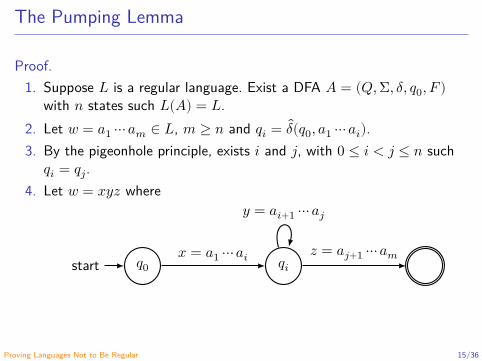
The Pumping Lemma
Proof.1. Suppose 𝐿 is a regular language. Exist a DFA 𝐴 = (𝑄, Σ, 𝛿, 𝑞0, 𝐹 )
with 𝑛 states such 𝐿(𝐴) = 𝐿.2. Let 𝑤 = 𝑎1 ⋯ 𝑎𝑚 ∈ 𝐿, 𝑚 ≥ 𝑛 and 𝑞𝑖 = 𝛿(𝑞0, 𝑎1 ⋯ 𝑎𝑖).3. By the pigeonhole principle, exists 𝑖 and 𝑗, with 0 ≤ 𝑖 < 𝑗 ≤ 𝑛 such
𝑞𝑖 = 𝑞𝑗.4. Let 𝑤 = 𝑥𝑦𝑧 where
𝑞0start 𝑞𝑖𝑥 = 𝑎1 ⋯ 𝑎𝑖
𝑦 = 𝑎𝑖+1 ⋯ 𝑎𝑗
𝑧 = 𝑎𝑗+1 ⋯ 𝑎𝑚
5. Then (∀𝑘 ≥ 0) 𝑥𝑦𝑘𝑧 ∈ 𝐿.
Proving Languages Not to Be Regular 15/36
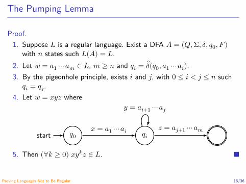
The Pumping Lemma
Proof.1. Suppose 𝐿 is a regular language. Exist a DFA 𝐴 = (𝑄, Σ, 𝛿, 𝑞0, 𝐹 )
with 𝑛 states such 𝐿(𝐴) = 𝐿.2. Let 𝑤 = 𝑎1 ⋯ 𝑎𝑚 ∈ 𝐿, 𝑚 ≥ 𝑛 and 𝑞𝑖 = 𝛿(𝑞0, 𝑎1 ⋯ 𝑎𝑖).3. By the pigeonhole principle, exists 𝑖 and 𝑗, with 0 ≤ 𝑖 < 𝑗 ≤ 𝑛 such
𝑞𝑖 = 𝑞𝑗.4. Let 𝑤 = 𝑥𝑦𝑧 where
𝑞0start 𝑞𝑖𝑥 = 𝑎1 ⋯ 𝑎𝑖
𝑦 = 𝑎𝑖+1 ⋯ 𝑎𝑗
𝑧 = 𝑎𝑗+1 ⋯ 𝑎𝑚
5. Then (∀𝑘 ≥ 0) 𝑥𝑦𝑘𝑧 ∈ 𝐿.
Proving Languages Not to Be Regular 16/36
Application of the Pumping Lemma: Proving LanguagesNot to Be Regular
MethodWhiteboard
Exercise (4.1.2.e)Let Σ = {0, 1} be an alphabet and let 𝐿 = {𝑤𝑤 ∣ 𝑤 ∈ Σ∗} be theso-called copy language. Prove that 𝐿 is not regular.
Proving Languages Not to Be Regular 17/36
Application of the Pumping Lemma: Proving LanguagesNot to Be Regular
MethodWhiteboard
Exercise (4.1.2.e)Let Σ = {0, 1} be an alphabet and let 𝐿 = {𝑤𝑤 ∣ 𝑤 ∈ Σ∗} be theso-called copy language. Prove that 𝐿 is not regular.
Proving Languages Not to Be Regular 18/36
Application of the Pumping Lemma: Proving LanguagesNot to Be Regular
Exercise (cont.)
Proof.1. Suppose 𝐿 is regular.
2. Let 𝑛 ∈ ℤ+ be a constant (according to the Pumping Lemma).3. Let 𝑤 = 0𝑛10𝑛1 ∈ 𝐿 and |𝑤| ≥ 𝑛.4. For the Pumping Lemma exists 𝑥, 𝑦 and 𝑧 such that 𝑤 = 𝑥𝑦𝑧,
|𝑥𝑦| ≤ 𝑛, 𝑦 ≠ 𝜀 and ∀𝑘 ≥ 0. 𝑥𝑦𝑘𝑧 ∈ 𝐿.5. Then 𝑦 = 0𝑚, 0 < 𝑚 ≤ 𝑛.6. But, 𝑥𝑦0𝑧 ∉ 𝐿 which is a contradiction by the Pumping Lemma.7. Therefore, 𝐿 is not regular.
Proving Languages Not to Be Regular 19/36
Application of the Pumping Lemma: Proving LanguagesNot to Be Regular
Exercise (cont.)
Proof.1. Suppose 𝐿 is regular.2. Let 𝑛 ∈ ℤ+ be a constant (according to the Pumping Lemma).
3. Let 𝑤 = 0𝑛10𝑛1 ∈ 𝐿 and |𝑤| ≥ 𝑛.4. For the Pumping Lemma exists 𝑥, 𝑦 and 𝑧 such that 𝑤 = 𝑥𝑦𝑧,
|𝑥𝑦| ≤ 𝑛, 𝑦 ≠ 𝜀 and ∀𝑘 ≥ 0. 𝑥𝑦𝑘𝑧 ∈ 𝐿.5. Then 𝑦 = 0𝑚, 0 < 𝑚 ≤ 𝑛.6. But, 𝑥𝑦0𝑧 ∉ 𝐿 which is a contradiction by the Pumping Lemma.7. Therefore, 𝐿 is not regular.
Proving Languages Not to Be Regular 20/36

Application of the Pumping Lemma: Proving LanguagesNot to Be Regular
Exercise (cont.)
Proof.1. Suppose 𝐿 is regular.2. Let 𝑛 ∈ ℤ+ be a constant (according to the Pumping Lemma).3. Let 𝑤 = 0𝑛10𝑛1 ∈ 𝐿 and |𝑤| ≥ 𝑛.
4. For the Pumping Lemma exists 𝑥, 𝑦 and 𝑧 such that 𝑤 = 𝑥𝑦𝑧,|𝑥𝑦| ≤ 𝑛, 𝑦 ≠ 𝜀 and ∀𝑘 ≥ 0. 𝑥𝑦𝑘𝑧 ∈ 𝐿.
5. Then 𝑦 = 0𝑚, 0 < 𝑚 ≤ 𝑛.6. But, 𝑥𝑦0𝑧 ∉ 𝐿 which is a contradiction by the Pumping Lemma.7. Therefore, 𝐿 is not regular.
Proving Languages Not to Be Regular 21/36

Application of the Pumping Lemma: Proving LanguagesNot to Be Regular
Exercise (cont.)
Proof.1. Suppose 𝐿 is regular.2. Let 𝑛 ∈ ℤ+ be a constant (according to the Pumping Lemma).3. Let 𝑤 = 0𝑛10𝑛1 ∈ 𝐿 and |𝑤| ≥ 𝑛.4. For the Pumping Lemma exists 𝑥, 𝑦 and 𝑧 such that 𝑤 = 𝑥𝑦𝑧,
|𝑥𝑦| ≤ 𝑛, 𝑦 ≠ 𝜀 and ∀𝑘 ≥ 0. 𝑥𝑦𝑘𝑧 ∈ 𝐿.
5. Then 𝑦 = 0𝑚, 0 < 𝑚 ≤ 𝑛.6. But, 𝑥𝑦0𝑧 ∉ 𝐿 which is a contradiction by the Pumping Lemma.7. Therefore, 𝐿 is not regular.
Proving Languages Not to Be Regular 22/36

Application of the Pumping Lemma: Proving LanguagesNot to Be Regular
Exercise (cont.)
Proof.1. Suppose 𝐿 is regular.2. Let 𝑛 ∈ ℤ+ be a constant (according to the Pumping Lemma).3. Let 𝑤 = 0𝑛10𝑛1 ∈ 𝐿 and |𝑤| ≥ 𝑛.4. For the Pumping Lemma exists 𝑥, 𝑦 and 𝑧 such that 𝑤 = 𝑥𝑦𝑧,
|𝑥𝑦| ≤ 𝑛, 𝑦 ≠ 𝜀 and ∀𝑘 ≥ 0. 𝑥𝑦𝑘𝑧 ∈ 𝐿.5. Then 𝑦 = 0𝑚, 0 < 𝑚 ≤ 𝑛.
6. But, 𝑥𝑦0𝑧 ∉ 𝐿 which is a contradiction by the Pumping Lemma.7. Therefore, 𝐿 is not regular.
Proving Languages Not to Be Regular 23/36
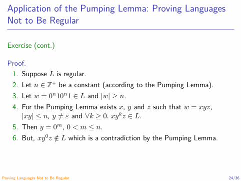
Application of the Pumping Lemma: Proving LanguagesNot to Be Regular
Exercise (cont.)
Proof.1. Suppose 𝐿 is regular.2. Let 𝑛 ∈ ℤ+ be a constant (according to the Pumping Lemma).3. Let 𝑤 = 0𝑛10𝑛1 ∈ 𝐿 and |𝑤| ≥ 𝑛.4. For the Pumping Lemma exists 𝑥, 𝑦 and 𝑧 such that 𝑤 = 𝑥𝑦𝑧,
|𝑥𝑦| ≤ 𝑛, 𝑦 ≠ 𝜀 and ∀𝑘 ≥ 0. 𝑥𝑦𝑘𝑧 ∈ 𝐿.5. Then 𝑦 = 0𝑚, 0 < 𝑚 ≤ 𝑛.6. But, 𝑥𝑦0𝑧 ∉ 𝐿 which is a contradiction by the Pumping Lemma.
7. Therefore, 𝐿 is not regular.
Proving Languages Not to Be Regular 24/36

Application of the Pumping Lemma: Proving LanguagesNot to Be Regular
Exercise (cont.)
Proof.1. Suppose 𝐿 is regular.2. Let 𝑛 ∈ ℤ+ be a constant (according to the Pumping Lemma).3. Let 𝑤 = 0𝑛10𝑛1 ∈ 𝐿 and |𝑤| ≥ 𝑛.4. For the Pumping Lemma exists 𝑥, 𝑦 and 𝑧 such that 𝑤 = 𝑥𝑦𝑧,
|𝑥𝑦| ≤ 𝑛, 𝑦 ≠ 𝜀 and ∀𝑘 ≥ 0. 𝑥𝑦𝑘𝑧 ∈ 𝐿.5. Then 𝑦 = 0𝑚, 0 < 𝑚 ≤ 𝑛.6. But, 𝑥𝑦0𝑧 ∉ 𝐿 which is a contradiction by the Pumping Lemma.7. Therefore, 𝐿 is not regular.
Proving Languages Not to Be Regular 25/36

Application of the Pumping Lemma: Proving LanguagesNot to Be Regular
Exercise (4.1.2.a)Let 𝐿 be the language
𝐿 = {0𝑛 ∣ 𝑛 is a perfect square}.
Prove that 𝐿 is not regular.
Proving Languages Not to Be Regular 26/36
Application of the Pumping Lemma: Proving LanguagesNot to Be Regular
Exercise (cont.)Proof.
1. Suppose 𝐿 is regular.
2. Let 𝑛 ∈ ℤ+ be a constant (according to the Pumping Lemma).3. Let 𝑤 = 0𝑛2 ∈ 𝐿 and |𝑤| ≥ 𝑛.4. For the Pumping Lemma exists 𝑥, 𝑦 and 𝑧 such that 𝑤 = 𝑥𝑦𝑧,
|𝑥𝑦| ≤ 𝑛, 𝑦 ≠ 𝜀 and ∀𝑘 ≥ 0. 𝑥𝑦𝑘𝑧 ∈ 𝐿.5. Then 𝑦 = 0𝑚, 0 < 𝑚 ≤ 𝑛 and 𝑛2 + 1 ≤ |𝑥𝑦𝑦𝑧| ≤ 𝑛2 + 𝑛.6. Since the next perfect square after 𝑛2 is (𝑛 + 1)2 = 𝑛2 + 2𝑛 + 1, we
know that 𝑥𝑦𝑦𝑧 ∉ 𝐿 (|𝑥𝑦𝑦𝑧| is strictly between the consecutiveperfect squares 𝑛2 and (𝑛 + 1)2).
7. This a contradiction by the Pumping Lemma.8. Therefore, 𝐿 is not regular.
Proving Languages Not to Be Regular 27/36
Application of the Pumping Lemma: Proving LanguagesNot to Be Regular
Exercise (cont.)Proof.
1. Suppose 𝐿 is regular.2. Let 𝑛 ∈ ℤ+ be a constant (according to the Pumping Lemma).
3. Let 𝑤 = 0𝑛2 ∈ 𝐿 and |𝑤| ≥ 𝑛.4. For the Pumping Lemma exists 𝑥, 𝑦 and 𝑧 such that 𝑤 = 𝑥𝑦𝑧,
|𝑥𝑦| ≤ 𝑛, 𝑦 ≠ 𝜀 and ∀𝑘 ≥ 0. 𝑥𝑦𝑘𝑧 ∈ 𝐿.5. Then 𝑦 = 0𝑚, 0 < 𝑚 ≤ 𝑛 and 𝑛2 + 1 ≤ |𝑥𝑦𝑦𝑧| ≤ 𝑛2 + 𝑛.6. Since the next perfect square after 𝑛2 is (𝑛 + 1)2 = 𝑛2 + 2𝑛 + 1, we
know that 𝑥𝑦𝑦𝑧 ∉ 𝐿 (|𝑥𝑦𝑦𝑧| is strictly between the consecutiveperfect squares 𝑛2 and (𝑛 + 1)2).
7. This a contradiction by the Pumping Lemma.8. Therefore, 𝐿 is not regular.
Proving Languages Not to Be Regular 28/36

Application of the Pumping Lemma: Proving LanguagesNot to Be Regular
Exercise (cont.)Proof.
1. Suppose 𝐿 is regular.2. Let 𝑛 ∈ ℤ+ be a constant (according to the Pumping Lemma).3. Let 𝑤 = 0𝑛2 ∈ 𝐿 and |𝑤| ≥ 𝑛.
4. For the Pumping Lemma exists 𝑥, 𝑦 and 𝑧 such that 𝑤 = 𝑥𝑦𝑧,|𝑥𝑦| ≤ 𝑛, 𝑦 ≠ 𝜀 and ∀𝑘 ≥ 0. 𝑥𝑦𝑘𝑧 ∈ 𝐿.
5. Then 𝑦 = 0𝑚, 0 < 𝑚 ≤ 𝑛 and 𝑛2 + 1 ≤ |𝑥𝑦𝑦𝑧| ≤ 𝑛2 + 𝑛.6. Since the next perfect square after 𝑛2 is (𝑛 + 1)2 = 𝑛2 + 2𝑛 + 1, we
know that 𝑥𝑦𝑦𝑧 ∉ 𝐿 (|𝑥𝑦𝑦𝑧| is strictly between the consecutiveperfect squares 𝑛2 and (𝑛 + 1)2).
7. This a contradiction by the Pumping Lemma.8. Therefore, 𝐿 is not regular.
Proving Languages Not to Be Regular 29/36
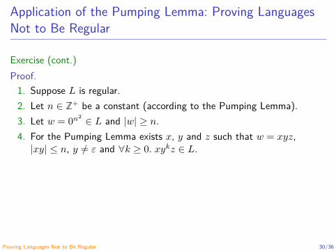
Application of the Pumping Lemma: Proving LanguagesNot to Be Regular
Exercise (cont.)Proof.
1. Suppose 𝐿 is regular.2. Let 𝑛 ∈ ℤ+ be a constant (according to the Pumping Lemma).3. Let 𝑤 = 0𝑛2 ∈ 𝐿 and |𝑤| ≥ 𝑛.4. For the Pumping Lemma exists 𝑥, 𝑦 and 𝑧 such that 𝑤 = 𝑥𝑦𝑧,
|𝑥𝑦| ≤ 𝑛, 𝑦 ≠ 𝜀 and ∀𝑘 ≥ 0. 𝑥𝑦𝑘𝑧 ∈ 𝐿.
5. Then 𝑦 = 0𝑚, 0 < 𝑚 ≤ 𝑛 and 𝑛2 + 1 ≤ |𝑥𝑦𝑦𝑧| ≤ 𝑛2 + 𝑛.6. Since the next perfect square after 𝑛2 is (𝑛 + 1)2 = 𝑛2 + 2𝑛 + 1, we
know that 𝑥𝑦𝑦𝑧 ∉ 𝐿 (|𝑥𝑦𝑦𝑧| is strictly between the consecutiveperfect squares 𝑛2 and (𝑛 + 1)2).
7. This a contradiction by the Pumping Lemma.8. Therefore, 𝐿 is not regular.
Proving Languages Not to Be Regular 30/36
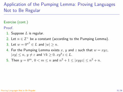
Application of the Pumping Lemma: Proving LanguagesNot to Be Regular
Exercise (cont.)Proof.
1. Suppose 𝐿 is regular.2. Let 𝑛 ∈ ℤ+ be a constant (according to the Pumping Lemma).3. Let 𝑤 = 0𝑛2 ∈ 𝐿 and |𝑤| ≥ 𝑛.4. For the Pumping Lemma exists 𝑥, 𝑦 and 𝑧 such that 𝑤 = 𝑥𝑦𝑧,
|𝑥𝑦| ≤ 𝑛, 𝑦 ≠ 𝜀 and ∀𝑘 ≥ 0. 𝑥𝑦𝑘𝑧 ∈ 𝐿.5. Then 𝑦 = 0𝑚, 0 < 𝑚 ≤ 𝑛 and 𝑛2 + 1 ≤ |𝑥𝑦𝑦𝑧| ≤ 𝑛2 + 𝑛.
6. Since the next perfect square after 𝑛2 is (𝑛 + 1)2 = 𝑛2 + 2𝑛 + 1, weknow that 𝑥𝑦𝑦𝑧 ∉ 𝐿 (|𝑥𝑦𝑦𝑧| is strictly between the consecutiveperfect squares 𝑛2 and (𝑛 + 1)2).
7. This a contradiction by the Pumping Lemma.8. Therefore, 𝐿 is not regular.
Proving Languages Not to Be Regular 31/36

Application of the Pumping Lemma: Proving LanguagesNot to Be Regular
Exercise (cont.)Proof.
1. Suppose 𝐿 is regular.2. Let 𝑛 ∈ ℤ+ be a constant (according to the Pumping Lemma).3. Let 𝑤 = 0𝑛2 ∈ 𝐿 and |𝑤| ≥ 𝑛.4. For the Pumping Lemma exists 𝑥, 𝑦 and 𝑧 such that 𝑤 = 𝑥𝑦𝑧,
|𝑥𝑦| ≤ 𝑛, 𝑦 ≠ 𝜀 and ∀𝑘 ≥ 0. 𝑥𝑦𝑘𝑧 ∈ 𝐿.5. Then 𝑦 = 0𝑚, 0 < 𝑚 ≤ 𝑛 and 𝑛2 + 1 ≤ |𝑥𝑦𝑦𝑧| ≤ 𝑛2 + 𝑛.6. Since the next perfect square after 𝑛2 is (𝑛 + 1)2 = 𝑛2 + 2𝑛 + 1, we
know that 𝑥𝑦𝑦𝑧 ∉ 𝐿 (|𝑥𝑦𝑦𝑧| is strictly between the consecutiveperfect squares 𝑛2 and (𝑛 + 1)2).
7. This a contradiction by the Pumping Lemma.8. Therefore, 𝐿 is not regular.
Proving Languages Not to Be Regular 32/36

Application of the Pumping Lemma: Proving LanguagesNot to Be Regular
Exercise (cont.)Proof.
1. Suppose 𝐿 is regular.2. Let 𝑛 ∈ ℤ+ be a constant (according to the Pumping Lemma).3. Let 𝑤 = 0𝑛2 ∈ 𝐿 and |𝑤| ≥ 𝑛.4. For the Pumping Lemma exists 𝑥, 𝑦 and 𝑧 such that 𝑤 = 𝑥𝑦𝑧,
|𝑥𝑦| ≤ 𝑛, 𝑦 ≠ 𝜀 and ∀𝑘 ≥ 0. 𝑥𝑦𝑘𝑧 ∈ 𝐿.5. Then 𝑦 = 0𝑚, 0 < 𝑚 ≤ 𝑛 and 𝑛2 + 1 ≤ |𝑥𝑦𝑦𝑧| ≤ 𝑛2 + 𝑛.6. Since the next perfect square after 𝑛2 is (𝑛 + 1)2 = 𝑛2 + 2𝑛 + 1, we
know that 𝑥𝑦𝑦𝑧 ∉ 𝐿 (|𝑥𝑦𝑦𝑧| is strictly between the consecutiveperfect squares 𝑛2 and (𝑛 + 1)2).
7. This a contradiction by the Pumping Lemma.
8. Therefore, 𝐿 is not regular.
Proving Languages Not to Be Regular 33/36
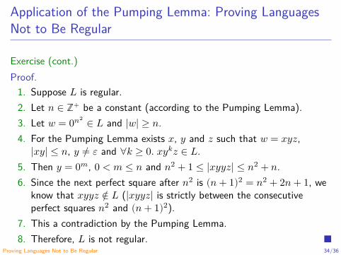
Application of the Pumping Lemma: Proving LanguagesNot to Be Regular
Exercise (cont.)Proof.
1. Suppose 𝐿 is regular.2. Let 𝑛 ∈ ℤ+ be a constant (according to the Pumping Lemma).3. Let 𝑤 = 0𝑛2 ∈ 𝐿 and |𝑤| ≥ 𝑛.4. For the Pumping Lemma exists 𝑥, 𝑦 and 𝑧 such that 𝑤 = 𝑥𝑦𝑧,
|𝑥𝑦| ≤ 𝑛, 𝑦 ≠ 𝜀 and ∀𝑘 ≥ 0. 𝑥𝑦𝑘𝑧 ∈ 𝐿.5. Then 𝑦 = 0𝑚, 0 < 𝑚 ≤ 𝑛 and 𝑛2 + 1 ≤ |𝑥𝑦𝑦𝑧| ≤ 𝑛2 + 𝑛.6. Since the next perfect square after 𝑛2 is (𝑛 + 1)2 = 𝑛2 + 2𝑛 + 1, we
know that 𝑥𝑦𝑦𝑧 ∉ 𝐿 (|𝑥𝑦𝑦𝑧| is strictly between the consecutiveperfect squares 𝑛2 and (𝑛 + 1)2).
7. This a contradiction by the Pumping Lemma.8. Therefore, 𝐿 is not regular.
Proving Languages Not to Be Regular 34/36
Proving Languages Not to Be Regular
RemarkFrishberg and Gasarch (2018) show other methods and some openproblems when proving that a language is not regular.
Proving Languages Not to Be Regular 35/36

References
Frishberg, D. and Gasarch, W. (2018). Open Problems Column. DifferentWays to Prove a Language is Not Regular. SIGACT News 49.1, pp. 40–54.doi: 10.1145/3197406.3197413 (cit. on p. 35).
Proving Languages Not to Be Regular 36/36

Automata and Formal Languages - CM0081Closure Properties of Regular Languages
Andrés Sicard-Ramírez
Universidad EAFIT
Semester 2018-1

Introduction
Let 𝐿 and 𝑀 be regular languages. The following languages are regular:
Union: 𝐿 ∪ 𝑀Intersection: 𝐿 ∩ 𝑀Complement: 𝐿Difference: 𝐿 − 𝑀Reversal: 𝐿𝑅 = {𝑤𝑟 ∈ Σ∗ ∣ 𝑤 ∈ 𝐿}Closure: 𝐿∗
Concatenation: 𝐿𝑀Homomorphism: ℎ(𝐿) = {ℎ(𝑤) ∣ 𝑤 ∈ 𝐿 and ℎ is a homomorphism}Inverse homomorphism:ℎ−1(𝐿) = {𝑤 ∈ Σ ∣ ℎ(𝑤) ∈ 𝐿 and ℎ is a homomorphism}
Closure Properties of Regular Languages 2/67
Introduction
Let 𝐿 and 𝑀 be regular languages. The following languages are regular:Union: 𝐿 ∪ 𝑀
Intersection: 𝐿 ∩ 𝑀Complement: 𝐿Difference: 𝐿 − 𝑀Reversal: 𝐿𝑅 = {𝑤𝑟 ∈ Σ∗ ∣ 𝑤 ∈ 𝐿}Closure: 𝐿∗
Concatenation: 𝐿𝑀Homomorphism: ℎ(𝐿) = {ℎ(𝑤) ∣ 𝑤 ∈ 𝐿 and ℎ is a homomorphism}Inverse homomorphism:ℎ−1(𝐿) = {𝑤 ∈ Σ ∣ ℎ(𝑤) ∈ 𝐿 and ℎ is a homomorphism}
Closure Properties of Regular Languages 3/67

Introduction
Let 𝐿 and 𝑀 be regular languages. The following languages are regular:Union: 𝐿 ∪ 𝑀Intersection: 𝐿 ∩ 𝑀
Complement: 𝐿Difference: 𝐿 − 𝑀Reversal: 𝐿𝑅 = {𝑤𝑟 ∈ Σ∗ ∣ 𝑤 ∈ 𝐿}Closure: 𝐿∗
Concatenation: 𝐿𝑀Homomorphism: ℎ(𝐿) = {ℎ(𝑤) ∣ 𝑤 ∈ 𝐿 and ℎ is a homomorphism}Inverse homomorphism:ℎ−1(𝐿) = {𝑤 ∈ Σ ∣ ℎ(𝑤) ∈ 𝐿 and ℎ is a homomorphism}
Closure Properties of Regular Languages 4/67

Introduction
Let 𝐿 and 𝑀 be regular languages. The following languages are regular:Union: 𝐿 ∪ 𝑀Intersection: 𝐿 ∩ 𝑀Complement: 𝐿
Difference: 𝐿 − 𝑀Reversal: 𝐿𝑅 = {𝑤𝑟 ∈ Σ∗ ∣ 𝑤 ∈ 𝐿}Closure: 𝐿∗
Concatenation: 𝐿𝑀Homomorphism: ℎ(𝐿) = {ℎ(𝑤) ∣ 𝑤 ∈ 𝐿 and ℎ is a homomorphism}Inverse homomorphism:ℎ−1(𝐿) = {𝑤 ∈ Σ ∣ ℎ(𝑤) ∈ 𝐿 and ℎ is a homomorphism}
Closure Properties of Regular Languages 5/67
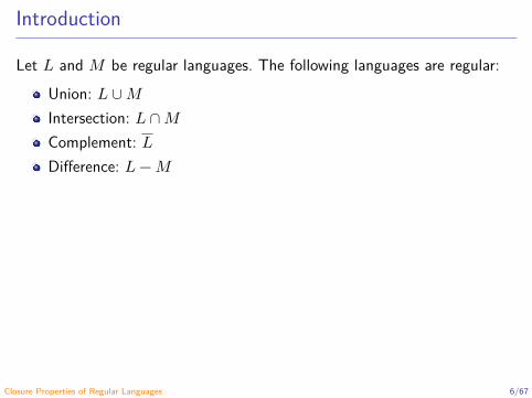
Introduction
Let 𝐿 and 𝑀 be regular languages. The following languages are regular:Union: 𝐿 ∪ 𝑀Intersection: 𝐿 ∩ 𝑀Complement: 𝐿Difference: 𝐿 − 𝑀
Reversal: 𝐿𝑅 = {𝑤𝑟 ∈ Σ∗ ∣ 𝑤 ∈ 𝐿}Closure: 𝐿∗
Concatenation: 𝐿𝑀Homomorphism: ℎ(𝐿) = {ℎ(𝑤) ∣ 𝑤 ∈ 𝐿 and ℎ is a homomorphism}Inverse homomorphism:ℎ−1(𝐿) = {𝑤 ∈ Σ ∣ ℎ(𝑤) ∈ 𝐿 and ℎ is a homomorphism}
Closure Properties of Regular Languages 6/67
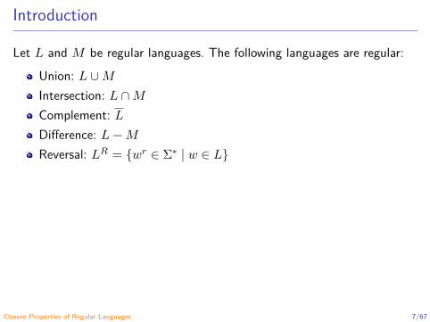
Introduction
Let 𝐿 and 𝑀 be regular languages. The following languages are regular:Union: 𝐿 ∪ 𝑀Intersection: 𝐿 ∩ 𝑀Complement: 𝐿Difference: 𝐿 − 𝑀Reversal: 𝐿𝑅 = {𝑤𝑟 ∈ Σ∗ ∣ 𝑤 ∈ 𝐿}
Closure: 𝐿∗
Concatenation: 𝐿𝑀Homomorphism: ℎ(𝐿) = {ℎ(𝑤) ∣ 𝑤 ∈ 𝐿 and ℎ is a homomorphism}Inverse homomorphism:ℎ−1(𝐿) = {𝑤 ∈ Σ ∣ ℎ(𝑤) ∈ 𝐿 and ℎ is a homomorphism}
Closure Properties of Regular Languages 7/67
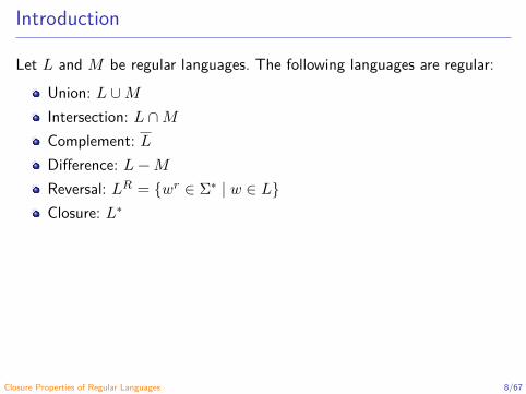
Introduction
Let 𝐿 and 𝑀 be regular languages. The following languages are regular:Union: 𝐿 ∪ 𝑀Intersection: 𝐿 ∩ 𝑀Complement: 𝐿Difference: 𝐿 − 𝑀Reversal: 𝐿𝑅 = {𝑤𝑟 ∈ Σ∗ ∣ 𝑤 ∈ 𝐿}Closure: 𝐿∗
Concatenation: 𝐿𝑀Homomorphism: ℎ(𝐿) = {ℎ(𝑤) ∣ 𝑤 ∈ 𝐿 and ℎ is a homomorphism}Inverse homomorphism:ℎ−1(𝐿) = {𝑤 ∈ Σ ∣ ℎ(𝑤) ∈ 𝐿 and ℎ is a homomorphism}
Closure Properties of Regular Languages 8/67

Introduction
Let 𝐿 and 𝑀 be regular languages. The following languages are regular:Union: 𝐿 ∪ 𝑀Intersection: 𝐿 ∩ 𝑀Complement: 𝐿Difference: 𝐿 − 𝑀Reversal: 𝐿𝑅 = {𝑤𝑟 ∈ Σ∗ ∣ 𝑤 ∈ 𝐿}Closure: 𝐿∗
Concatenation: 𝐿𝑀
Homomorphism: ℎ(𝐿) = {ℎ(𝑤) ∣ 𝑤 ∈ 𝐿 and ℎ is a homomorphism}Inverse homomorphism:ℎ−1(𝐿) = {𝑤 ∈ Σ ∣ ℎ(𝑤) ∈ 𝐿 and ℎ is a homomorphism}
Closure Properties of Regular Languages 9/67

Introduction
Let 𝐿 and 𝑀 be regular languages. The following languages are regular:Union: 𝐿 ∪ 𝑀Intersection: 𝐿 ∩ 𝑀Complement: 𝐿Difference: 𝐿 − 𝑀Reversal: 𝐿𝑅 = {𝑤𝑟 ∈ Σ∗ ∣ 𝑤 ∈ 𝐿}Closure: 𝐿∗
Concatenation: 𝐿𝑀Homomorphism: ℎ(𝐿) = {ℎ(𝑤) ∣ 𝑤 ∈ 𝐿 and ℎ is a homomorphism}
Inverse homomorphism:ℎ−1(𝐿) = {𝑤 ∈ Σ ∣ ℎ(𝑤) ∈ 𝐿 and ℎ is a homomorphism}
Closure Properties of Regular Languages 10/67
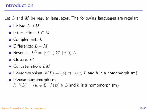
Introduction
Let 𝐿 and 𝑀 be regular languages. The following languages are regular:Union: 𝐿 ∪ 𝑀Intersection: 𝐿 ∩ 𝑀Complement: 𝐿Difference: 𝐿 − 𝑀Reversal: 𝐿𝑅 = {𝑤𝑟 ∈ Σ∗ ∣ 𝑤 ∈ 𝐿}Closure: 𝐿∗
Concatenation: 𝐿𝑀Homomorphism: ℎ(𝐿) = {ℎ(𝑤) ∣ 𝑤 ∈ 𝐿 and ℎ is a homomorphism}Inverse homomorphism:ℎ−1(𝐿) = {𝑤 ∈ Σ ∣ ℎ(𝑤) ∈ 𝐿 and ℎ is a homomorphism}
Closure Properties of Regular Languages 11/67

Closure Under Union and Complementation
Theorem (4.4)If 𝐿 and 𝑀 are regular languages, then so is 𝐿 ∪ 𝑀 .
Proof(Using regular expressions)
Closure Properties of Regular Languages 12/67
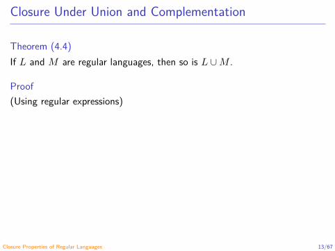
Closure Under Union and Complementation
Theorem (4.4)If 𝐿 and 𝑀 are regular languages, then so is 𝐿 ∪ 𝑀 .
Proof(Using regular expressions)
Closure Properties of Regular Languages 13/67
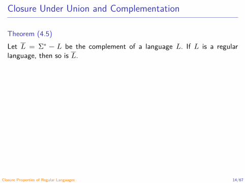
Closure Under Union and Complementation
Theorem (4.5)Let 𝐿 = Σ∗ − 𝐿 be the complement of a language 𝐿. If 𝐿 is a regularlanguage, then so is 𝐿.
Proof.Let
𝐴 = (𝑄, Σ, 𝛿, 𝑞0, 𝐹 )
be a DFA such that 𝐿(𝐴) = 𝐿. Then
𝐵 = (𝑄, Σ, 𝛿, 𝑞0, 𝑄 − 𝐹)
is a DFA such 𝐿(𝐵) = 𝐿.
Closure Properties of Regular Languages 14/67

Closure Under Union and Complementation
Theorem (4.5)Let 𝐿 = Σ∗ − 𝐿 be the complement of a language 𝐿. If 𝐿 is a regularlanguage, then so is 𝐿.
Proof.Let
𝐴 = (𝑄, Σ, 𝛿, 𝑞0, 𝐹 )
be a DFA such that 𝐿(𝐴) = 𝐿. Then
𝐵 = (𝑄, Σ, 𝛿, 𝑞0, 𝑄 − 𝐹)
is a DFA such 𝐿(𝐵) = 𝐿.
Closure Properties of Regular Languages 15/67

Closure Under Union and Complementation
Question: “Do you see how to take a regular expression and change it intoone that defines the complement language?” (Hopcroft, Motwani andUllman 2007, p. 136)
Closure Properties of Regular Languages 16/67

Closure Under Union and Complementation
Using the closure properties we can prove that a language is not regular.
ExampleGiven that
𝐿= = {𝑤 ∈ {0, 1}∗ ∣ 𝑤 has an equal numbers of 0’s and 1’s}
is a language not regular. Prove that
𝐿≠ = {𝑤 ∈ {0, 1}∗ ∣ 𝑤 has an unequal numbers of 0’s and 1’s}
is a language not regular.
ProofWhiteboard.
Closure Properties of Regular Languages 17/67
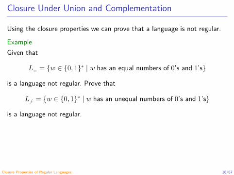
Closure Under Union and Complementation
Using the closure properties we can prove that a language is not regular.
ExampleGiven that
𝐿= = {𝑤 ∈ {0, 1}∗ ∣ 𝑤 has an equal numbers of 0’s and 1’s}
is a language not regular. Prove that
𝐿≠ = {𝑤 ∈ {0, 1}∗ ∣ 𝑤 has an unequal numbers of 0’s and 1’s}
is a language not regular.
ProofWhiteboard.
Closure Properties of Regular Languages 18/67
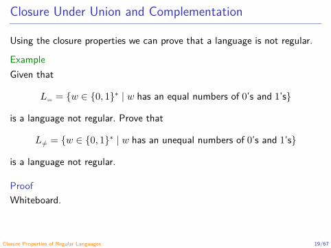
Closure Under Union and Complementation
Using the closure properties we can prove that a language is not regular.
ExampleGiven that
𝐿= = {𝑤 ∈ {0, 1}∗ ∣ 𝑤 has an equal numbers of 0’s and 1’s}
is a language not regular. Prove that
𝐿≠ = {𝑤 ∈ {0, 1}∗ ∣ 𝑤 has an unequal numbers of 0’s and 1’s}
is a language not regular.
ProofWhiteboard.
Closure Properties of Regular Languages 19/67

Product Construction
Let 𝐴𝐿, 𝐴𝑀 and 𝐴 be DFAs given by
𝐴𝐿 = (𝑄𝐿, Σ, 𝛿𝐿, 𝑞𝐿, 𝐹𝐿),𝐴𝑀 = (𝑄𝑀 , Σ, 𝛿𝑀 , 𝑞𝑀 , 𝐹𝑀),
𝐴 = (𝑄𝐿 × 𝑄𝑀 , Σ, 𝛿, (𝑞𝐿, 𝑞𝑀), 𝐹𝐿 × 𝐹𝑀),
where
𝛿 ∶ (𝑄𝐿 × 𝑄𝑀) × Σ → 𝑄𝐿 × 𝑄𝑀𝛿((𝑝, 𝑞), 𝑎) = (𝛿𝐿(𝑝, 𝑎), 𝛿𝑀(𝑞, 𝑎)).
Theorem (Exercise 4.2.15)For all 𝑤 ∈ Σ∗,
𝛿((𝑞𝐿, 𝑞𝑀), 𝑤) = ( 𝛿𝐿(𝑞𝐿, 𝑤), 𝛿𝑀(𝑞𝑀 , 𝑤)).
Closure Properties of Regular Languages 20/67
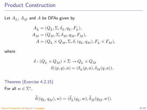
Product Construction
Let 𝐴𝐿, 𝐴𝑀 and 𝐴 be DFAs given by
𝐴𝐿 = (𝑄𝐿, Σ, 𝛿𝐿, 𝑞𝐿, 𝐹𝐿),𝐴𝑀 = (𝑄𝑀 , Σ, 𝛿𝑀 , 𝑞𝑀 , 𝐹𝑀),
𝐴 = (𝑄𝐿 × 𝑄𝑀 , Σ, 𝛿, (𝑞𝐿, 𝑞𝑀), 𝐹𝐿 × 𝐹𝑀),
where
𝛿 ∶ (𝑄𝐿 × 𝑄𝑀) × Σ → 𝑄𝐿 × 𝑄𝑀𝛿((𝑝, 𝑞), 𝑎) = (𝛿𝐿(𝑝, 𝑎), 𝛿𝑀(𝑞, 𝑎)).
Theorem (Exercise 4.2.15)For all 𝑤 ∈ Σ∗,
𝛿((𝑞𝐿, 𝑞𝑀), 𝑤) = ( 𝛿𝐿(𝑞𝐿, 𝑤), 𝛿𝑀(𝑞𝑀 , 𝑤)).
Closure Properties of Regular Languages 21/67

Product Construction
Proof by induction on 𝑤.1. Basis step
𝛿((𝑞𝐿, 𝑞𝑀), 𝜀) = (𝑞𝐿, 𝑞𝑀) (def. of 𝛿)= ( 𝛿𝐿(𝑞𝐿, 𝜀), 𝛿𝑀(𝑞𝑀 , 𝜀)) (def. of 𝛿𝐿 and 𝛿𝑀)
2. Inductive step
𝛿((𝑞𝐿, 𝑞𝑀), 𝑥𝑎)= 𝛿( 𝛿((𝑞𝐿, 𝑞𝑀), 𝑥), 𝑎) (def. of 𝛿)= 𝛿(( 𝛿𝐿(𝑞𝐿, 𝑥), 𝛿𝑀(𝑞𝑀 , 𝑥)), 𝑎) (by IH)= (𝛿𝐿( 𝛿𝐿(𝑞𝐿, 𝑥), 𝑎), 𝛿𝑀( 𝛿𝑀(𝑞𝑀 , 𝑥), 𝑎)) (def. of 𝛿)= ( 𝛿𝐿(𝑞𝐿, 𝑥𝑎), 𝛿𝑀(𝑞𝑀 , 𝑥𝑎)) (def. of 𝛿𝐿 and 𝛿𝐿)
Closure Properties of Regular Languages 22/67
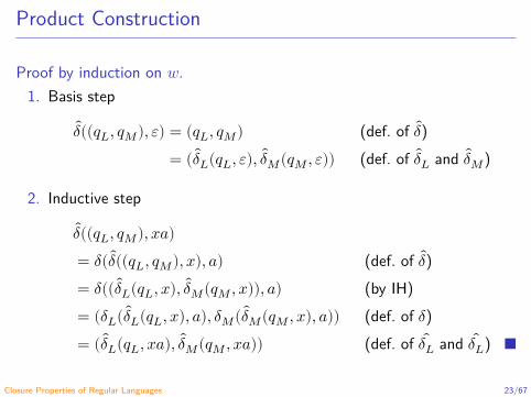
Product Construction
Proof by induction on 𝑤.1. Basis step
𝛿((𝑞𝐿, 𝑞𝑀), 𝜀) = (𝑞𝐿, 𝑞𝑀) (def. of 𝛿)= ( 𝛿𝐿(𝑞𝐿, 𝜀), 𝛿𝑀(𝑞𝑀 , 𝜀)) (def. of 𝛿𝐿 and 𝛿𝑀)
2. Inductive step
𝛿((𝑞𝐿, 𝑞𝑀), 𝑥𝑎)= 𝛿( 𝛿((𝑞𝐿, 𝑞𝑀), 𝑥), 𝑎) (def. of 𝛿)= 𝛿(( 𝛿𝐿(𝑞𝐿, 𝑥), 𝛿𝑀(𝑞𝑀 , 𝑥)), 𝑎) (by IH)= (𝛿𝐿( 𝛿𝐿(𝑞𝐿, 𝑥), 𝑎), 𝛿𝑀( 𝛿𝑀(𝑞𝑀 , 𝑥), 𝑎)) (def. of 𝛿)= ( 𝛿𝐿(𝑞𝐿, 𝑥𝑎), 𝛿𝑀(𝑞𝑀 , 𝑥𝑎)) (def. of 𝛿𝐿 and 𝛿𝐿)
Closure Properties of Regular Languages 23/67

Closure Under Intersection
Theorem (4.8)If 𝐿 and 𝑀 are regular languages, then so is 𝐿 ∩ 𝑀 .
Proof.Let 𝐴𝐿 and 𝐴𝑀 be DFAs accepting 𝐿 and 𝑀 . The product constructionof 𝐴𝐿 and 𝐴𝑀 accepts 𝐿 ∩ 𝑀 .
Different proof.The regular languages are closure under union and complement, and
𝐿 ∩ 𝑀 = 𝐿 ∪ 𝑀.
Closure Properties of Regular Languages 24/67
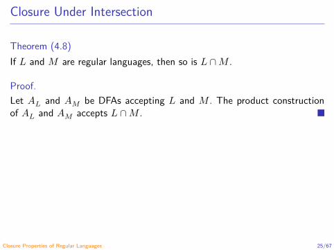
Closure Under Intersection
Theorem (4.8)If 𝐿 and 𝑀 are regular languages, then so is 𝐿 ∩ 𝑀 .
Proof.Let 𝐴𝐿 and 𝐴𝑀 be DFAs accepting 𝐿 and 𝑀 . The product constructionof 𝐴𝐿 and 𝐴𝑀 accepts 𝐿 ∩ 𝑀 .
Different proof.The regular languages are closure under union and complement, and
𝐿 ∩ 𝑀 = 𝐿 ∪ 𝑀.
Closure Properties of Regular Languages 25/67

Closure Under Intersection
Theorem (4.8)If 𝐿 and 𝑀 are regular languages, then so is 𝐿 ∩ 𝑀 .
Proof.Let 𝐴𝐿 and 𝐴𝑀 be DFAs accepting 𝐿 and 𝑀 . The product constructionof 𝐴𝐿 and 𝐴𝑀 accepts 𝐿 ∩ 𝑀 .
Different proof.The regular languages are closure under union and complement, and
𝐿 ∩ 𝑀 = 𝐿 ∪ 𝑀.
Closure Properties of Regular Languages 26/67

Closure Under Reversal
DefinitionLet 𝑤 = 𝑎1𝑎2 ⋯ 𝑎𝑛 be a word. The reversal of 𝑤 is defined by
𝑤𝑅 = 𝑎𝑛𝑎𝑛−1 ⋯ 𝑎1.
DefinitionLet 𝐿 be a language on alphabet Σ. The reversal of 𝐿 is defined by
𝐿𝑅 = {𝑤𝑅 ∈ Σ∗ ∣ 𝑤 ∈ 𝐿}.
Theorem (4.11)If 𝐿 is regular language, then so is 𝐿𝑅 (proof using automata or regularexpressions)
Closure Properties of Regular Languages 27/67
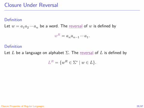
Closure Under Reversal
DefinitionLet 𝑤 = 𝑎1𝑎2 ⋯ 𝑎𝑛 be a word. The reversal of 𝑤 is defined by
𝑤𝑅 = 𝑎𝑛𝑎𝑛−1 ⋯ 𝑎1.
DefinitionLet 𝐿 be a language on alphabet Σ. The reversal of 𝐿 is defined by
𝐿𝑅 = {𝑤𝑅 ∈ Σ∗ ∣ 𝑤 ∈ 𝐿}.
Theorem (4.11)If 𝐿 is regular language, then so is 𝐿𝑅 (proof using automata or regularexpressions)
Closure Properties of Regular Languages 28/67
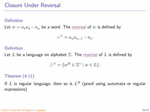
Closure Under Reversal
DefinitionLet 𝑤 = 𝑎1𝑎2 ⋯ 𝑎𝑛 be a word. The reversal of 𝑤 is defined by
𝑤𝑅 = 𝑎𝑛𝑎𝑛−1 ⋯ 𝑎1.
DefinitionLet 𝐿 be a language on alphabet Σ. The reversal of 𝐿 is defined by
𝐿𝑅 = {𝑤𝑅 ∈ Σ∗ ∣ 𝑤 ∈ 𝐿}.
Theorem (4.11)If 𝐿 is regular language, then so is 𝐿𝑅 (proof using automata or regularexpressions)
Closure Properties of Regular Languages 29/67
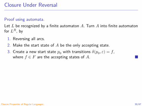
Closure Under Reversal
Proof using automata.Let 𝐿 be recognized by a finite automaton 𝐴. Turn 𝐴 into finite automatonfor 𝐿𝑅, by
1. Reversing all arcs.2. Make the start state of 𝐴 be the only accepting state.3. Create a new start state 𝑝0 with transitions 𝛿(𝑝0, 𝜀) = 𝑓 ,
where 𝑓 ∈ 𝐹 are the accepting states of 𝐴.
Closure Properties of Regular Languages 30/67
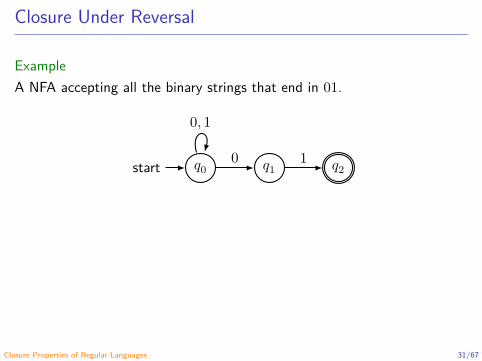
Closure Under Reversal
ExampleA NFA accepting all the binary strings that end in 01.
𝑞0start 𝑞1 𝑞2
0, 1
0 1
A NFA accepting all the binary strings that start with 10.
𝑞0 𝑞1 𝑞2 𝑝0 start
0, 1
0 1 𝜀
Closure Properties of Regular Languages 31/67
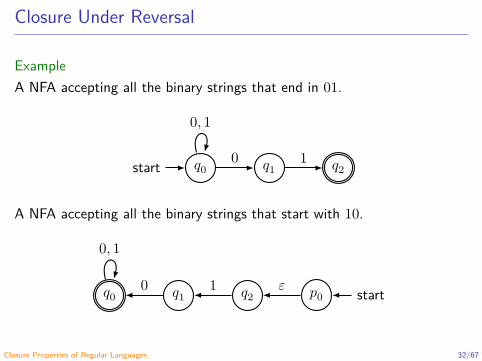
Closure Under Reversal
ExampleA NFA accepting all the binary strings that end in 01.
𝑞0start 𝑞1 𝑞2
0, 1
0 1
A NFA accepting all the binary strings that start with 10.
𝑞0 𝑞1 𝑞2 𝑝0 start
0, 1
0 1 𝜀
Closure Properties of Regular Languages 32/67
Homomorphisms
DefinitionAn algebraic structure on a set 𝐴 ≠ ∅ is essentially a collection of 𝑛-aryoperations on 𝐴 (Birkhoff 1946, 1987).
Example (Semigroup)A semigroup (𝑆, ∗) is a set 𝑆 with an associative binary operation∗ ∶ 𝑆 × 𝑆 → 𝑆.
Example (Monoid)A monoid (𝑀, ∗, 𝜀) is a semigroup (𝑀, ∗) with an element 𝜀 ∈ 𝑀 which isan unit for ∗, i.e. ∀𝑥. 𝑥 ∗ 𝜀 = 𝜀 ∗ 𝑥 = 𝑥.
Closure Properties of Regular Languages 33/67
Homomorphisms
DefinitionAn algebraic structure on a set 𝐴 ≠ ∅ is essentially a collection of 𝑛-aryoperations on 𝐴 (Birkhoff 1946, 1987).
Example (Semigroup)A semigroup (𝑆, ∗) is a set 𝑆 with an associative binary operation∗ ∶ 𝑆 × 𝑆 → 𝑆.
Example (Monoid)A monoid (𝑀, ∗, 𝜀) is a semigroup (𝑀, ∗) with an element 𝜀 ∈ 𝑀 which isan unit for ∗, i.e. ∀𝑥. 𝑥 ∗ 𝜀 = 𝜀 ∗ 𝑥 = 𝑥.
Closure Properties of Regular Languages 34/67

Homomorphisms
DefinitionAn algebraic structure on a set 𝐴 ≠ ∅ is essentially a collection of 𝑛-aryoperations on 𝐴 (Birkhoff 1946, 1987).
Example (Semigroup)A semigroup (𝑆, ∗) is a set 𝑆 with an associative binary operation∗ ∶ 𝑆 × 𝑆 → 𝑆.
Example (Monoid)A monoid (𝑀, ∗, 𝜀) is a semigroup (𝑀, ∗) with an element 𝜀 ∈ 𝑀 which isan unit for ∗, i.e. ∀𝑥. 𝑥 ∗ 𝜀 = 𝜀 ∗ 𝑥 = 𝑥.
Closure Properties of Regular Languages 35/67

Homomorphisms
DefinitionA homomorphism is a structure-preserving map between two algebraic struc-tures.
ExampleA homomorphism between two semigroups (𝑆, ∗) and (𝑆′, ∗′) is a function𝜑 ∶ 𝑆 → 𝑆′ such that:
∀𝑥 𝑦. 𝜑(𝑥 ∗ 𝑦) = 𝜑(𝑥) ∗′ 𝜑(𝑦).
Graphically (see whiteboard).
Closure Properties of Regular Languages 36/67
Homomorphisms
DefinitionA homomorphism is a structure-preserving map between two algebraic struc-tures.
ExampleA homomorphism between two semigroups (𝑆, ∗) and (𝑆′, ∗′) is a function𝜑 ∶ 𝑆 → 𝑆′ such that:
∀𝑥 𝑦. 𝜑(𝑥 ∗ 𝑦) = 𝜑(𝑥) ∗′ 𝜑(𝑦).
Graphically (see whiteboard).
Closure Properties of Regular Languages 37/67

Homomorphisms
ExampleA homomorphism between two monoids (𝑀, ∗, 𝜀) and (𝑀 ′, ∗′, 𝜀′) is afunction 𝜑 ∶ 𝑀 → 𝑀 ′ such that:
∀𝑥 𝑦. 𝜑(𝑥 ∗ 𝑦) = 𝜑(𝑥) ∗′ 𝜑(𝑦),𝜑(𝜀) = 𝜀′.
Closure Properties of Regular Languages 38/67

Homomorphisms
DefinitionA homomorphism 𝜑 between two algebraic structures is (Cohn 1981):
a monomorphism if 𝜑 is an injection,an epimorphism if 𝜑 is a surjection,an endomorphism if 𝜑 is from an algebraic structure to itself,an isomorphism if 𝜑 is a bijection,an automorphism if 𝜑 is a bijective endomorphism.
Closure Properties of Regular Languages 39/67

Closure Under Homomorphism
DefinitionLet Σ and Γ be two alphabets. A homomorphism between (Σ∗, ·, 𝜀) and(Γ∗, ·, 𝜀) is a function
ℎ ∶ Σ∗ → Γ∗
𝑎1𝑎2 ⋯ 𝑎𝑛 ↦ ℎ(𝑎1)ℎ(𝑎2) ⋯ ℎ(𝑎𝑛)𝜀 ↦ 𝜀
Note: For this reason the textbook talk about a homomorphism ℎ ∶ Σ → Γ∗.
Closure Properties of Regular Languages 40/67
Closure Under Homomorphism
ExampleLet ℎ ∶ {0, 1}∗ → {𝑎, 𝑏}∗ be a homomorphism defined by
ℎ(0) = 𝑎𝑏,ℎ(1) = 𝜀.
Then
ℎ(0011) = ℎ(0)ℎ(0)ℎ(1)ℎ(1)= 𝑎𝑏𝑎𝑏.
Closure Properties of Regular Languages 41/67
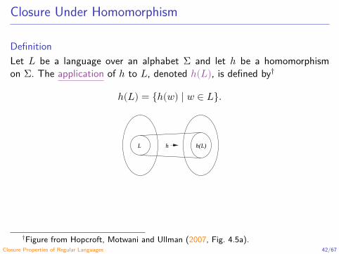
Closure Under Homomorphism
DefinitionLet 𝐿 be a language over an alphabet Σ and let ℎ be a homomorphismon Σ. The application of ℎ to 𝐿, denoted ℎ(𝐿), is defined by†
ℎ(𝐿) = {ℎ(𝑤) ∣ 𝑤 ∈ 𝐿}.
Inverse Homomorphism
Let h : Σ∗ → Θ∗ be a homom. Let L ⊆ Θ∗,and define
h−1(L) = {w ∈ Σ∗ : h(w) ∈ L}
L h(L)
Lh-1 (L)
(a)
(b)
h
h
110
†Figure from Hopcroft, Motwani and Ullman (2007, Fig. 4.5a).Closure Properties of Regular Languages 42/67

Closure Under Homomorphism
ExampleLet ℎ ∶ {0, 1}∗ → {𝑎, 𝑏}∗ be a homomorphism defined by
ℎ(0) = 𝑎𝑏,ℎ(1) = 𝜀.
If 𝐿 = 𝐿(10∗1), then ℎ(𝐿) = 𝐿((ab)∗).
Closure Properties of Regular Languages 43/67

Closure Under Homomorphism
Theorem (4.14)If 𝐿 is a regular language over the alphabet Σ and ℎ is a homomorphismon Σ, then ℎ(𝐿) is also regular.
Proof planLet 𝐸 be a regular expression such 𝐿 = 𝐿(𝐸).Let ℎ(𝐸) be the regular expression replacing each symbol 𝑎 ∈ Σby ℎ(𝑎) in the regular expression 𝐸.We need to prove that 𝐿(ℎ(𝐸)) = ℎ(𝐿(𝐸)).
Closure Properties of Regular Languages 44/67
Closure Under Homomorphism
Theorem (4.14)If 𝐿 is a regular language over the alphabet Σ and ℎ is a homomorphismon Σ, then ℎ(𝐿) is also regular.
Proof planLet 𝐸 be a regular expression such 𝐿 = 𝐿(𝐸).Let ℎ(𝐸) be the regular expression replacing each symbol 𝑎 ∈ Σby ℎ(𝑎) in the regular expression 𝐸.We need to prove that 𝐿(ℎ(𝐸)) = ℎ(𝐿(𝐸)).
Closure Properties of Regular Languages 45/67

Closure Under Homomorphism
Proving 𝐿(ℎ(𝐸)) = ℎ(𝐿(𝐸)).Basis step
𝐸 is 𝜀 or ∅.1. ℎ(𝐸) = 𝐸 (ℎ does not affect 𝐸)2. ℎ(𝐿(𝐸)) = 𝐿(𝐸) (𝐿(𝐸) is empty or only contains 𝜀)3. 𝐿(ℎ(𝐸)) = 𝐿(𝐸) = ℎ(𝐿(𝐸)) (by 1 and 2)
𝐸 = a1. 𝐿(𝐸) = {𝑎}2. ℎ(𝐿(𝐸)) = {ℎ(𝑎)}3. ℎ(𝐸) is the regular expression that is the string of symbols ℎ(𝑎)4. 𝐿(ℎ(𝐸)) = {ℎ(𝑎)}5. 𝐿(ℎ(𝐸)) = ℎ(𝐿(𝐸)) (by transitivity between 2 and 4)
Closure Properties of Regular Languages 46/67
Closure Under Homomorphism
Proving 𝐿(ℎ(𝐸)) = ℎ(𝐿(𝐸)).Basis step
𝐸 is 𝜀 or ∅.1. ℎ(𝐸) = 𝐸 (ℎ does not affect 𝐸)2. ℎ(𝐿(𝐸)) = 𝐿(𝐸) (𝐿(𝐸) is empty or only contains 𝜀)3. 𝐿(ℎ(𝐸)) = 𝐿(𝐸) = ℎ(𝐿(𝐸)) (by 1 and 2)
𝐸 = a1. 𝐿(𝐸) = {𝑎}2. ℎ(𝐿(𝐸)) = {ℎ(𝑎)}3. ℎ(𝐸) is the regular expression that is the string of symbols ℎ(𝑎)4. 𝐿(ℎ(𝐸)) = {ℎ(𝑎)}5. 𝐿(ℎ(𝐸)) = ℎ(𝐿(𝐸)) (by transitivity between 2 and 4)
Closure Properties of Regular Languages 47/67

Closure Under Homomorphism
Proving 𝐿(ℎ(𝐸)) = ℎ(𝐿(𝐸)).Inductive step
𝐸 = 𝐹 + 𝐺1. 𝐿(𝐸) = 𝐿(𝐹) ∪ 𝐿(𝐺) (def. of +)2. ℎ(𝐸) = ℎ(𝐹 + 𝐺) = ℎ(𝐹) + ℎ(𝐺) (def. of ℎ(𝐸))3. 𝐿(ℎ(𝐸)) = 𝐿(ℎ(𝐹) + ℎ(𝐺)) = 𝐿(ℎ(𝐹)) ∪ 𝐿(ℎ(𝐺)) (def. of +)4. ℎ(𝐿(𝐸)) = ℎ(𝐿(𝐹) ∪ 𝐿(𝐺)) = ℎ(𝐿(𝐹)) ∪ ℎ(𝐿(𝐺)) (ℎ is applied
to a language by application to each of its strings)5. 𝐿(ℎ(𝐹)) = ℎ(𝐿(𝐹) and 𝐿(ℎ(𝐺)) = ℎ(𝐿(𝐺) (IH)6. 𝐿(ℎ(𝐸)) = ℎ(𝐿(𝐸))
Closure Properties of Regular Languages 48/67
Closure Under Homomorphism
Proving 𝐿(ℎ(𝐸)) = ℎ(𝐿(𝐸)).Inductive step (cont.)
𝐸 = 𝐹𝐺 (similar to the previous case)
𝐸 = 𝐹 ∗ (similar to the previous case)1. 𝐿(𝐸) = (𝐿(𝐹))∗ (def. of ∗)2. ℎ(𝐸) = ℎ(𝐹 ∗) = (ℎ(𝐹))∗ (def. of ℎ(𝐸))3. 𝐿(ℎ(𝐸)) = 𝐿((ℎ(𝐹))∗) = (𝐿(ℎ(𝐹)))∗ (def. of ∗)4. ℎ(𝐿(𝐸)) = ℎ((𝐿(𝐹))∗) = (ℎ(𝐿(𝐹)))∗ (ℎ is applied to a language
by application to each of its strings)5. 𝐿(ℎ(𝐹)) = ℎ(𝐿(𝐹)) (IH)6. 𝐿(ℎ(𝐸)) = ℎ(𝐿(𝐸))
Closure Properties of Regular Languages 49/67

Closure Under Homomorphism
Proving 𝐿(ℎ(𝐸)) = ℎ(𝐿(𝐸)).Inductive step (cont.)
𝐸 = 𝐹𝐺 (similar to the previous case)𝐸 = 𝐹 ∗ (similar to the previous case)
1. 𝐿(𝐸) = (𝐿(𝐹))∗ (def. of ∗)2. ℎ(𝐸) = ℎ(𝐹 ∗) = (ℎ(𝐹))∗ (def. of ℎ(𝐸))3. 𝐿(ℎ(𝐸)) = 𝐿((ℎ(𝐹))∗) = (𝐿(ℎ(𝐹)))∗ (def. of ∗)4. ℎ(𝐿(𝐸)) = ℎ((𝐿(𝐹))∗) = (ℎ(𝐿(𝐹)))∗ (ℎ is applied to a language
by application to each of its strings)5. 𝐿(ℎ(𝐹)) = ℎ(𝐿(𝐹)) (IH)6. 𝐿(ℎ(𝐸)) = ℎ(𝐿(𝐸))
Closure Properties of Regular Languages 50/67
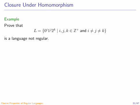
Closure Under Homomorphism
ExampleProve that
𝐿 = {0𝑖1𝑗2𝑘 ∣ 𝑖, 𝑗, 𝑘 ∈ ℤ+ and 𝑖 ≠ 𝑗 ≠ 𝑘}is a language not regular.
Proof.1. We define the homomorphism
ℎ(0) = 0, ℎ(1) = 1, ℎ(2) = 𝜀.
2. The homomorphism ℎ removes the 2𝑘s, so
ℎ(𝐿) = {0𝑖1𝑗 ∣ 𝑖, 𝑗 ∈ ℤ+ and 𝑖 ≠ 𝑗}.
3. We know that ℎ(𝐿) is not regular, so 𝐿 is not regular.
Closure Properties of Regular Languages 51/67

Closure Under Homomorphism
ExampleProve that
𝐿 = {0𝑖1𝑗2𝑘 ∣ 𝑖, 𝑗, 𝑘 ∈ ℤ+ and 𝑖 ≠ 𝑗 ≠ 𝑘}is a language not regular.
Proof.1. We define the homomorphism
ℎ(0) = 0, ℎ(1) = 1, ℎ(2) = 𝜀.
2. The homomorphism ℎ removes the 2𝑘s, so
ℎ(𝐿) = {0𝑖1𝑗 ∣ 𝑖, 𝑗 ∈ ℤ+ and 𝑖 ≠ 𝑗}.
3. We know that ℎ(𝐿) is not regular, so 𝐿 is not regular.
Closure Properties of Regular Languages 52/67

Closure Under Homomorphism
ExampleProve that
𝐿 = {0𝑖1𝑗2𝑘 ∣ 𝑖, 𝑗, 𝑘 ∈ ℤ+ and 𝑖 ≠ 𝑗 ≠ 𝑘}is a language not regular.
Proof.1. We define the homomorphism
ℎ(0) = 0, ℎ(1) = 1, ℎ(2) = 𝜀.
2. The homomorphism ℎ removes the 2𝑘s, so
ℎ(𝐿) = {0𝑖1𝑗 ∣ 𝑖, 𝑗 ∈ ℤ+ and 𝑖 ≠ 𝑗}.
3. We know that ℎ(𝐿) is not regular, so 𝐿 is not regular.
Closure Properties of Regular Languages 53/67
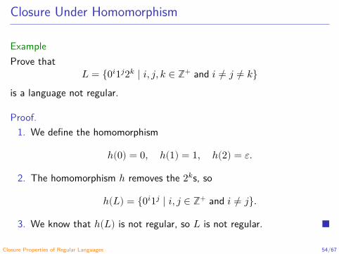
Closure Under Homomorphism
ExampleProve that
𝐿 = {0𝑖1𝑗2𝑘 ∣ 𝑖, 𝑗, 𝑘 ∈ ℤ+ and 𝑖 ≠ 𝑗 ≠ 𝑘}is a language not regular.
Proof.1. We define the homomorphism
ℎ(0) = 0, ℎ(1) = 1, ℎ(2) = 𝜀.
2. The homomorphism ℎ removes the 2𝑘s, so
ℎ(𝐿) = {0𝑖1𝑗 ∣ 𝑖, 𝑗 ∈ ℤ+ and 𝑖 ≠ 𝑗}.
3. We know that ℎ(𝐿) is not regular, so 𝐿 is not regular.
Closure Properties of Regular Languages 54/67

Closure Under Homomorphism
ExampleLet 𝐿 be a regular language and ℎ a homomorphism on 𝐿. Define ℎ∗(𝐿) by
ℎ∗(𝐿) = 𝐿 ∪ ℎ(𝐿) ∪ ℎ(ℎ(𝐿)) ∪ ℎ(ℎ(ℎ(𝐿))) ∪ …
Is ℎ∗(𝐿) necessarily regular?
No. Let 𝐿 = {01} and ℎ defined as ℎ(0) = 00 and ℎ(1) = 11. Then
ℎ∗(𝐿) = {01, 0011, 00001111, … }= {0𝑛1𝑛 ∣ 𝑛 = 2𝑘 for 𝑘 ≥ 0},
which is a language not regular.†
†From somewhere in Internet (I don’t remember).Closure Properties of Regular Languages 55/67

Closure Under Homomorphism
ExampleLet 𝐿 be a regular language and ℎ a homomorphism on 𝐿. Define ℎ∗(𝐿) by
ℎ∗(𝐿) = 𝐿 ∪ ℎ(𝐿) ∪ ℎ(ℎ(𝐿)) ∪ ℎ(ℎ(ℎ(𝐿))) ∪ …
Is ℎ∗(𝐿) necessarily regular?No. Let 𝐿 = {01} and ℎ defined as ℎ(0) = 00 and ℎ(1) = 11. Then
ℎ∗(𝐿) = {01, 0011, 00001111, … }= {0𝑛1𝑛 ∣ 𝑛 = 2𝑘 for 𝑘 ≥ 0},
which is a language not regular.†
†From somewhere in Internet (I don’t remember).Closure Properties of Regular Languages 56/67

Closure Under Inverse Homomorphism
DefinitionLet ℎ ∶ Σ∗ → Γ∗ be a homomorphism and 𝐿 ⊆ Γ∗ a language. Theapplication of ℎ−1 to 𝐿, denoted ℎ−1(𝐿), is defined by†
ℎ−1(𝐿) = {𝑤 ∈ Σ∗ ∣ ℎ(𝑤) ∈ 𝐿}.
Inverse Homomorphism
Let h : Σ∗ → Θ∗ be a homom. Let L ⊆ Θ∗,and define
h−1(L) = {w ∈ Σ∗ : h(w) ∈ L}
L h(L)
Lh-1 (L)
(a)
(b)
h
h
110RemarkNote that ℎ−1 is a relation but it is not necessarily a function.
†Figure from Hopcroft, Motwani and Ullman (2007, Fig. 4.5b).Closure Properties of Regular Languages 57/67
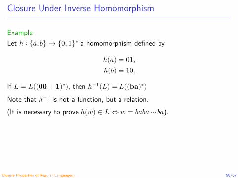
Closure Under Inverse Homomorphism
ExampleLet ℎ ∶ {𝑎, 𝑏} → {0, 1}∗ a homomorphism defined by
ℎ(𝑎) = 01,ℎ(𝑏) = 10.
If 𝐿 = 𝐿((00 + 1)∗), then ℎ−1(𝐿) = 𝐿((ba)∗)Note that ℎ−1 is not a function, but a relation.(It is necessary to prove ℎ(𝑤) ∈ 𝐿 ⇔ 𝑤 = 𝑏𝑎𝑏𝑎 ⋯ 𝑏𝑎).
Closure Properties of Regular Languages 58/67
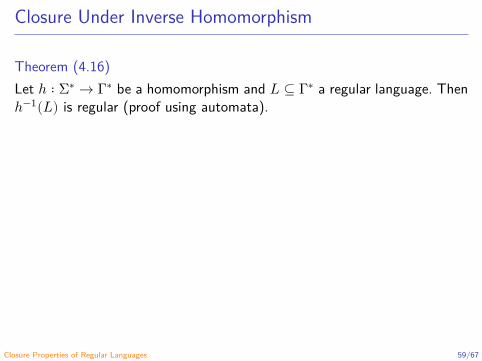
Closure Under Inverse Homomorphism
Theorem (4.16)Let ℎ ∶ Σ∗ → Γ∗ be a homomorphism and 𝐿 ⊆ Γ∗ a regular language. Thenℎ−1(𝐿) is regular (proof using automata).
Closure Properties of Regular Languages 59/67

Closure Under Inverse Homomorphism
ExampleProve that 𝐿 = {0𝑛12𝑛 ∣ 𝑛 ≥ 0} is a language not regular.
Proof.1. Given the homomorphism
ℎ(0) = 0,ℎ(1) = 11,
then ℎ−1(𝐿) = {0𝑛1𝑛 ∣ 𝑛 ≥ 0}.2. Since ℎ−1(𝐿) is not regular, then 𝐿 is not regular.
Closure Properties of Regular Languages 60/67
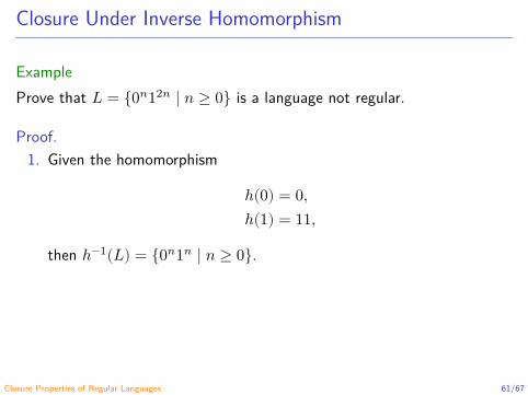
Closure Under Inverse Homomorphism
ExampleProve that 𝐿 = {0𝑛12𝑛 ∣ 𝑛 ≥ 0} is a language not regular.
Proof.1. Given the homomorphism
ℎ(0) = 0,ℎ(1) = 11,
then ℎ−1(𝐿) = {0𝑛1𝑛 ∣ 𝑛 ≥ 0}.
2. Since ℎ−1(𝐿) is not regular, then 𝐿 is not regular.
Closure Properties of Regular Languages 61/67

Closure Under Inverse Homomorphism
ExampleProve that 𝐿 = {0𝑛12𝑛 ∣ 𝑛 ≥ 0} is a language not regular.
Proof.1. Given the homomorphism
ℎ(0) = 0,ℎ(1) = 11,
then ℎ−1(𝐿) = {0𝑛1𝑛 ∣ 𝑛 ≥ 0}.2. Since ℎ−1(𝐿) is not regular, then 𝐿 is not regular.
Closure Properties of Regular Languages 62/67
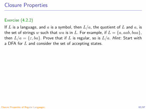
Closure Properties
Exercise (4.2.2)If 𝐿 is a language, and 𝑎 is a symbol, then 𝐿/𝑎, the quotient of 𝐿 and 𝑎, isthe set of strings 𝑤 such that 𝑤𝑎 is in 𝐿. For example, if 𝐿 = {𝑎, 𝑎𝑎𝑏, 𝑏𝑎𝑎},then 𝐿/𝑎 = {𝜀, 𝑏𝑎}. Prove that if 𝐿 is regular, so is 𝐿/𝑎. Hint: Start witha DFA for 𝐿 and consider the set of accepting states.
Proof (Hopcroft, Motwani and Ullman (2007) solution).Start with a DFA 𝐴 for 𝐿. Construct a new DFA 𝐵, that is exactly the sameas 𝐴, except that state 𝑞 is an accepting state of 𝐵 if and only if 𝛿(𝑞, 𝑎)is an accepting state of 𝐴. Then 𝐵 accepts input string 𝑤 if and only if 𝐴accepts 𝑤𝑎; that is, 𝐿(𝐵) = 𝐿/𝑎.
Closure Properties of Regular Languages 63/67

Closure Properties
Exercise (4.2.2)If 𝐿 is a language, and 𝑎 is a symbol, then 𝐿/𝑎, the quotient of 𝐿 and 𝑎, isthe set of strings 𝑤 such that 𝑤𝑎 is in 𝐿. For example, if 𝐿 = {𝑎, 𝑎𝑎𝑏, 𝑏𝑎𝑎},then 𝐿/𝑎 = {𝜀, 𝑏𝑎}. Prove that if 𝐿 is regular, so is 𝐿/𝑎. Hint: Start witha DFA for 𝐿 and consider the set of accepting states.
Proof (Hopcroft, Motwani and Ullman (2007) solution).Start with a DFA 𝐴 for 𝐿. Construct a new DFA 𝐵, that is exactly the sameas 𝐴, except that state 𝑞 is an accepting state of 𝐵 if and only if 𝛿(𝑞, 𝑎)is an accepting state of 𝐴. Then 𝐵 accepts input string 𝑤 if and only if 𝐴accepts 𝑤𝑎; that is, 𝐿(𝐵) = 𝐿/𝑎.
Closure Properties of Regular Languages 64/67

Closure Properties
Exercise (4.2.3)If 𝐿 is a language, and 𝑎 is a symbol, then 𝑎\𝐿 is the set of strings 𝑤 suchthat 𝑎𝑤 is in 𝐿. For example, if 𝐿 = {𝑎, 𝑎𝑎𝑏, 𝑏𝑎𝑎}, then 𝑎\𝐿 = {𝜀, 𝑎𝑏}.Prove that if 𝐿 is regular, so is 𝑎\𝐿. Hint: Start with a DFA for 𝐿 andconsider its start state.
Proof (Hopcroft, Motwani and Ullman (2007) solution).Start with a DFA 𝐴 for 𝐿. Construct a new DFA 𝐵, that is exactly thesame as 𝐴, except that its start state is 𝛿(𝑞0, 𝑎) where 𝑞0 is the start stateof 𝐴. Then 𝐵 accepts input string 𝑤 if and only if 𝐴 accepts 𝑎𝑤; that is,𝐿(𝐵) = 𝐿\𝑎.
Closure Properties of Regular Languages 65/67
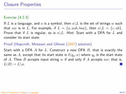
Closure Properties
Exercise (4.2.3)If 𝐿 is a language, and 𝑎 is a symbol, then 𝑎\𝐿 is the set of strings 𝑤 suchthat 𝑎𝑤 is in 𝐿. For example, if 𝐿 = {𝑎, 𝑎𝑎𝑏, 𝑏𝑎𝑎}, then 𝑎\𝐿 = {𝜀, 𝑎𝑏}.Prove that if 𝐿 is regular, so is 𝑎\𝐿. Hint: Start with a DFA for 𝐿 andconsider its start state.Proof (Hopcroft, Motwani and Ullman (2007) solution).Start with a DFA 𝐴 for 𝐿. Construct a new DFA 𝐵, that is exactly thesame as 𝐴, except that its start state is 𝛿(𝑞0, 𝑎) where 𝑞0 is the start stateof 𝐴. Then 𝐵 accepts input string 𝑤 if and only if 𝐴 accepts 𝑎𝑤; that is,𝐿(𝐵) = 𝐿\𝑎.
Closure Properties of Regular Languages 66/67

References
Birkhoff, G. (1946). Universal Algebra. In: Comptes Rendus du PremierCongrès Canadien de Mathématiques. University of Toronto Press,pp. 310–326 (cit. on pp. 33–35).— (1987). Universal Algebra. In: Selected Papers on Algebra andTopology by Garrett Birkhoff. Ed. by Rota, G.-C. and Oliveira, J. S.Birkhäuser, pp. 146–162 (cit. on pp. 33–35).Cohn, P. M. (1981). Universal Algebra. Revised edition. D. ReidelPublishing Company (cit. on p. 39).Hopcroft, J. E., Motwani, R. and Ullman, J. D. (2007). Introduction toAutomata theory, Languages, and Computation. 3rd ed. Pearson Education(cit. on pp. 16, 42, 57, 63–66).
Closure Properties of Regular Languages 67/67
Automata and Formal Languages - CM0081Problems That Computers Cannot Solve
Andrés Sicard-Ramírez
Universidad EAFIT
Semester 2018-1

Undecidable Problems
RecallGiven 𝐿 ⊆ Σ∗ and a word 𝑤 ∈ Σ∗, to recall that to decide whether or not𝑤 ∈ 𝐿 is a (decision) problem on 𝐿.
Definition (informally)A problem is undecidable if no program can solve it.
Are there undecidable problems?Yes! (by cardinality)
1. {𝐿 ∣ 𝐿 ⊆ Σ∗} is not enumerable.2. {𝑃 ∣ 𝑃 is a program} is enumerable (lexicographical order).3. There are more languages than programs.4. Therefore, there must be undecidable problems.
Problems That Computers Cannot Solve 2/38

Undecidable Problems
RecallGiven 𝐿 ⊆ Σ∗ and a word 𝑤 ∈ Σ∗, to recall that to decide whether or not𝑤 ∈ 𝐿 is a (decision) problem on 𝐿.
Definition (informally)A problem is undecidable if no program can solve it.
Are there undecidable problems?
Yes! (by cardinality)1. {𝐿 ∣ 𝐿 ⊆ Σ∗} is not enumerable.2. {𝑃 ∣ 𝑃 is a program} is enumerable (lexicographical order).3. There are more languages than programs.4. Therefore, there must be undecidable problems.
Problems That Computers Cannot Solve 3/38

Undecidable Problems
RecallGiven 𝐿 ⊆ Σ∗ and a word 𝑤 ∈ Σ∗, to recall that to decide whether or not𝑤 ∈ 𝐿 is a (decision) problem on 𝐿.
Definition (informally)A problem is undecidable if no program can solve it.
Are there undecidable problems?Yes! (by cardinality)
1. {𝐿 ∣ 𝐿 ⊆ Σ∗} is not enumerable.2. {𝑃 ∣ 𝑃 is a program} is enumerable (lexicographical order).3. There are more languages than programs.4. Therefore, there must be undecidable problems.
Problems That Computers Cannot Solve 4/38
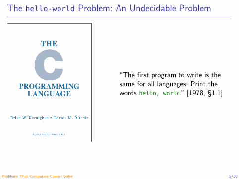
The hello-world Problem: An Undecidable Problem
“The first program to write is thesame for all languages: Print thewords hello, world.” [1978, §1.1]
Problems That Computers Cannot Solve 5/38
The hello-world Problem
The hello-world problemTo determine whether a given program, with a given input, prints hello,world as the first 12 characters that it prints.
TheoremThe hello-world problem is an undecidable problem.
Problems That Computers Cannot Solve 6/38
The hello-world Problem
The hello-world problemTo determine whether a given program, with a given input, prints hello,world as the first 12 characters that it prints.
TheoremThe hello-world problem is an undecidable problem.
Problems That Computers Cannot Solve 7/38

The hello-world Problem
Informal proof1. We assume that the program H exists:
hello-word tester
H
P Yes
I No
Problems That Computers Cannot Solve 8/38
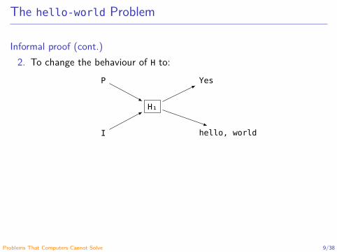
The hello-world Problem
Informal proof (cont.)2. To change the behaviour of H to:
H₁
P Yes
I hello, world
Problems That Computers Cannot Solve 9/38

The hello-world Problem
Informal proof (cont.)3. Restrict H₁ to take only input P (i.e. P is the input of the program P):
H₂P
Yes
hello, world
Problems That Computers Cannot Solve 10/38
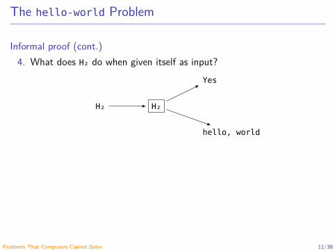
The hello-world Problem
Informal proof (cont.)4. What does H₂ do when given itself as input?
H₂H₂
Yes
hello, world
Therefore, the program H₂ cannot exist.5. Therefore, the program H cannot exists.
Problems That Computers Cannot Solve 11/38

The hello-world Problem
Informal proof (cont.)4. What does H₂ do when given itself as input?
H₂H₂
Yes
hello, world
Therefore, the program H₂ cannot exist.
5. Therefore, the program H cannot exists.
Problems That Computers Cannot Solve 12/38

The hello-world Problem
Informal proof (cont.)4. What does H₂ do when given itself as input?
H₂H₂
Yes
hello, world
Therefore, the program H₂ cannot exist.5. Therefore, the program H cannot exists.
Problems That Computers Cannot Solve 13/38

Computability: Historical Remarks
1900 David Hilbert’s problemsWir müssen wissen — wir werden wissen!(We must know — we will know!)
1931 Kurt Gödel’s undecidability theorems
1936 The year of the confluence!𝜆-calculus (Alonzo Church, Stephen Kleene)Partial recursive functions (Kurt Gödel)Post machines (Emil Post)Turing machines (Alan Turing)
1936–40 The Church-Turing thesis: A (number-theoretic) function iseffectively calculable if and only if there is a Turing machinewhich computes it.
Problems That Computers Cannot Solve 14/38
Computability: Historical Remarks
1900 David Hilbert’s problemsWir müssen wissen — wir werden wissen!(We must know — we will know!)
1931 Kurt Gödel’s undecidability theorems
1936 The year of the confluence!𝜆-calculus (Alonzo Church, Stephen Kleene)Partial recursive functions (Kurt Gödel)Post machines (Emil Post)Turing machines (Alan Turing)
1936–40 The Church-Turing thesis: A (number-theoretic) function iseffectively calculable if and only if there is a Turing machinewhich computes it.
Problems That Computers Cannot Solve 15/38
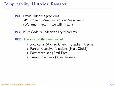
Computability: Historical Remarks
1900 David Hilbert’s problemsWir müssen wissen — wir werden wissen!(We must know — we will know!)
1931 Kurt Gödel’s undecidability theorems
1936 The year of the confluence!𝜆-calculus (Alonzo Church, Stephen Kleene)Partial recursive functions (Kurt Gödel)Post machines (Emil Post)Turing machines (Alan Turing)
1936–40 The Church-Turing thesis: A (number-theoretic) function iseffectively calculable if and only if there is a Turing machinewhich computes it.
Problems That Computers Cannot Solve 16/38

Computability: Historical Remarks
1900 David Hilbert’s problemsWir müssen wissen — wir werden wissen!(We must know — we will know!)
1931 Kurt Gödel’s undecidability theorems
1936 The year of the confluence!𝜆-calculus (Alonzo Church, Stephen Kleene)Partial recursive functions (Kurt Gödel)Post machines (Emil Post)Turing machines (Alan Turing)
1936–40 The Church-Turing thesis: A (number-theoretic) function iseffectively calculable if and only if there is a Turing machinewhich computes it.
Problems That Computers Cannot Solve 17/38
Computability: Historical Remarks (cont.)
1985 Deutsch’s quantum Turing machine
1940–Today Many equivalents models of computation
Problems That Computers Cannot Solve 18/38
Computability: Historical Remarks (cont.)
1985 Deutsch’s quantum Turing machine1940–Today Many equivalents models of computation
Problems That Computers Cannot Solve 19/38
Problems Reduction
How to prove that a problem is undecidable?Proof of negation
Problem reductionReduction from a problem 𝑃1 to a problem 𝑃2:
yes
no
yes
no
𝑃1 𝑃2
Problems That Computers Cannot Solve 20/38
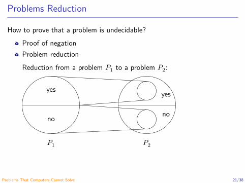
Problems Reduction
How to prove that a problem is undecidable?Proof of negationProblem reductionReduction from a problem 𝑃1 to a problem 𝑃2:
yes
no
yes
no
𝑃1 𝑃2
Problems That Computers Cannot Solve 21/38

Problems Reduction
TheoremIf 𝑃1 is undecidable and there is a reduction of 𝑃1 to 𝑃2, then 𝑃2 is unde-cidable too.
Proof by contradiction.
reduction decide𝑃1 instance 𝑃2 instance
no
yes
1. Let’s suppose 𝑃2 decidable2. There is a reduction from 𝑃1 to 𝑃2
⇒ 𝑃1 decidable⇒ ⊥ (contradiction)
3. Therefore, 𝑃2 is undecidable
Problems That Computers Cannot Solve 22/38
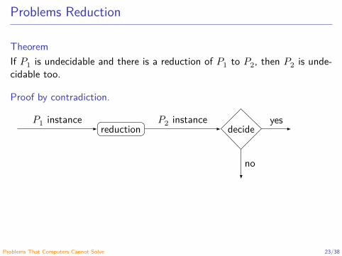
Problems Reduction
TheoremIf 𝑃1 is undecidable and there is a reduction of 𝑃1 to 𝑃2, then 𝑃2 is unde-cidable too.
Proof by contradiction.
reduction decide𝑃1 instance 𝑃2 instance
no
yes
1. Let’s suppose 𝑃2 decidable2. There is a reduction from 𝑃1 to 𝑃2
⇒ 𝑃1 decidable⇒ ⊥ (contradiction)
3. Therefore, 𝑃2 is undecidable
Problems That Computers Cannot Solve 23/38
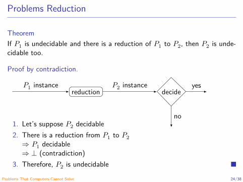
Problems Reduction
TheoremIf 𝑃1 is undecidable and there is a reduction of 𝑃1 to 𝑃2, then 𝑃2 is unde-cidable too.
Proof by contradiction.
reduction decide𝑃1 instance 𝑃2 instance
no
yes
1. Let’s suppose 𝑃2 decidable2. There is a reduction from 𝑃1 to 𝑃2
⇒ 𝑃1 decidable⇒ ⊥ (contradiction)
3. Therefore, 𝑃2 is undecidable
Problems That Computers Cannot Solve 24/38
Problems Reduction
Example (The calls-foo problem)Problem: Does a program Q with an input z calls the function foo?
Prove that the calls-foo problem is undecidable.
Problems That Computers Cannot Solve 25/38
Problems Reduction
Example (The calls-foo problem)Problem: Does a program Q with an input z calls the function foo?Prove that the calls-foo problem is undecidable.
Problems That Computers Cannot Solve 26/38
Problems Reduction
Example (cont.)
Proof.Idea: Reduction of the hello-world problem to the calls-foo problem.
That is, P with input y prints hello, world iff Q with input z calls thefunction foo.Reduction:
1. P₁: Rename foo in P.2. P₂: Add foo to P₁.3. P₃: Save the first 12 characters that prints P₂.4. P₄: When P₃ executes an output statement if output is hello, world
then calls foo.5. Q = P₄ and y = z.
Problems That Computers Cannot Solve 27/38

Problems Reduction
Example (cont.)
Proof.Idea: Reduction of the hello-world problem to the calls-foo problem.That is, P with input y prints hello, world iff Q with input z calls thefunction foo.
Reduction:1. P₁: Rename foo in P.2. P₂: Add foo to P₁.3. P₃: Save the first 12 characters that prints P₂.4. P₄: When P₃ executes an output statement if output is hello, world
then calls foo.5. Q = P₄ and y = z.
Problems That Computers Cannot Solve 28/38
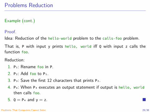
Problems Reduction
Example (cont.)
Proof.Idea: Reduction of the hello-world problem to the calls-foo problem.That is, P with input y prints hello, world iff Q with input z calls thefunction foo.Reduction:
1. P₁: Rename foo in P.2. P₂: Add foo to P₁.3. P₃: Save the first 12 characters that prints P₂.4. P₄: When P₃ executes an output statement if output is hello, world
then calls foo.5. Q = P₄ and y = z.
Problems That Computers Cannot Solve 29/38
Problems Reduction
Exercise (The halting problem, 8.1.1.a)Problem: Given a program and an input, does the program eventuallyhalt; i.e., does the program not loop forever on the input?
Prove that the halting problem is undecidable.
Problems That Computers Cannot Solve 30/38
Problems Reduction
Exercise (The halting problem, 8.1.1.a)Problem: Given a program and an input, does the program eventuallyhalt; i.e., does the program not loop forever on the input?Prove that the halting problem is undecidable.
Problems That Computers Cannot Solve 31/38
Problems Reduction
Exercise (cont.)
Proof (based on the solutions to Hopcroft, Motwani and Ullman (2007)).Idea: Reduction of the hello-world problem to the halting problem.
That is, P with input y prints hello, world iff Q with input z halt.Reduction:
1. P₁: Add an infinite loop (e.g. while(1){x=x;}) to the end of main.2. P₂: Save the first 12 characters that prints P₁.3. P₃: When P₂ executes an output statement if output is hello, world
then P₃ halts by going to the end of main.4. Q = P₃ and y = z.
Problems That Computers Cannot Solve 32/38
Problems Reduction
Exercise (cont.)
Proof (based on the solutions to Hopcroft, Motwani and Ullman (2007)).Idea: Reduction of the hello-world problem to the halting problem.That is, P with input y prints hello, world iff Q with input z halt.
Reduction:1. P₁: Add an infinite loop (e.g. while(1){x=x;}) to the end of main.2. P₂: Save the first 12 characters that prints P₁.3. P₃: When P₂ executes an output statement if output is hello, world
then P₃ halts by going to the end of main.4. Q = P₃ and y = z.
Problems That Computers Cannot Solve 33/38

Problems Reduction
Exercise (cont.)
Proof (based on the solutions to Hopcroft, Motwani and Ullman (2007)).Idea: Reduction of the hello-world problem to the halting problem.That is, P with input y prints hello, world iff Q with input z halt.Reduction:
1. P₁: Add an infinite loop (e.g. while(1){x=x;}) to the end of main.2. P₂: Save the first 12 characters that prints P₁.3. P₃: When P₂ executes an output statement if output is hello, world
then P₃ halts by going to the end of main.4. Q = P₃ and y = z.
Problems That Computers Cannot Solve 34/38

Problems Reduction
TheoremIf 𝑃1 is undecidable and there is a reduction of 𝑃1 to 𝑃2, then 𝑃2 is unde-cidable too.Be careful! The reduction is from 𝑃1 to 𝑃2, it is not from 𝑃2 to 𝑃1:
From a reduction of 𝑃1 to 𝑃2:
𝑃2 decidable ⇒ 𝑃1 decidable𝑃1 undecidable ⇒ 𝑃2 undecidable
From a reduction of 𝑃2 to 𝑃1:
𝑃1 decidable ⇒ 𝑃2 decidable (hypothesis false)𝑃2 undecidable ⇒ 𝑃1 undecidable (hypothesis unknown)
Problems That Computers Cannot Solve 35/38

Problems Reduction
TheoremIf 𝑃1 is undecidable and there is a reduction of 𝑃1 to 𝑃2, then 𝑃2 is unde-cidable too.Be careful! The reduction is from 𝑃1 to 𝑃2, it is not from 𝑃2 to 𝑃1:
From a reduction of 𝑃1 to 𝑃2:
𝑃2 decidable ⇒ 𝑃1 decidable𝑃1 undecidable ⇒ 𝑃2 undecidable
From a reduction of 𝑃2 to 𝑃1:
𝑃1 decidable ⇒ 𝑃2 decidable (hypothesis false)𝑃2 undecidable ⇒ 𝑃1 undecidable (hypothesis unknown)
Problems That Computers Cannot Solve 36/38
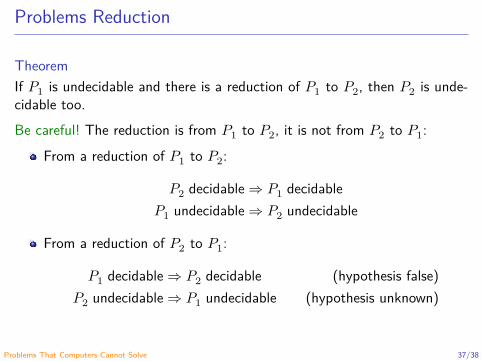
Problems Reduction
TheoremIf 𝑃1 is undecidable and there is a reduction of 𝑃1 to 𝑃2, then 𝑃2 is unde-cidable too.Be careful! The reduction is from 𝑃1 to 𝑃2, it is not from 𝑃2 to 𝑃1:
From a reduction of 𝑃1 to 𝑃2:
𝑃2 decidable ⇒ 𝑃1 decidable𝑃1 undecidable ⇒ 𝑃2 undecidable
From a reduction of 𝑃2 to 𝑃1:
𝑃1 decidable ⇒ 𝑃2 decidable (hypothesis false)𝑃2 undecidable ⇒ 𝑃1 undecidable (hypothesis unknown)
Problems That Computers Cannot Solve 37/38
References
Hopcroft, J. E., Motwani, R. and Ullman, J. D. (2007). Introduction toAutomata theory, Languages, and Computation. 3rd ed. Pearson Education(cit. on pp. 32–34).
Problems That Computers Cannot Solve 38/38

Automata and Formal Languages - CM0081Turing Machines
Andrés Sicard-Ramírez
Universidad EAFIT
Semester 2018-1

Turing Machines
Alan Mathison Turing(1912 – 1954)
Turing Machines 2/45
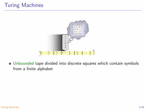
Turing Machines
Unbounded tape divided into discrete squares which contain symbolsfrom a finite alphabet
Read/Write headFinite set of instructions (transition function)Move of a Turing machine (tape symbol under the head, currentstate): change state, rewrite the symbol and move the head onesquare
Turing Machines 3/45
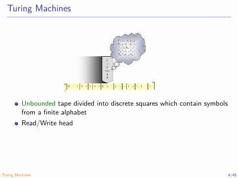
Turing Machines
Unbounded tape divided into discrete squares which contain symbolsfrom a finite alphabetRead/Write head
Finite set of instructions (transition function)Move of a Turing machine (tape symbol under the head, currentstate): change state, rewrite the symbol and move the head onesquare
Turing Machines 4/45
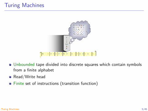
Turing Machines
Unbounded tape divided into discrete squares which contain symbolsfrom a finite alphabetRead/Write headFinite set of instructions (transition function)
Move of a Turing machine (tape symbol under the head, currentstate): change state, rewrite the symbol and move the head onesquare
Turing Machines 5/45

Turing Machines
Unbounded tape divided into discrete squares which contain symbolsfrom a finite alphabetRead/Write headFinite set of instructions (transition function)Move of a Turing machine (tape symbol under the head, currentstate): change state, rewrite the symbol and move the head onesquare
Turing Machines 6/45
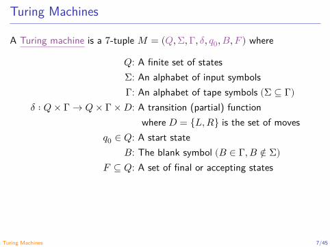
Turing Machines
A Turing machine is a 7-tuple 𝑀 = (𝑄, Σ, Γ, 𝛿, 𝑞0, 𝐵, 𝐹) where
𝑄: A finite set of statesΣ: An alphabet of input symbolsΓ: An alphabet of tape symbols (Σ ⊆ Γ)
𝛿 ∶ 𝑄 × Γ → 𝑄 × Γ × 𝐷: A transition (partial) functionwhere 𝐷 = {𝐿, 𝑅} is the set of moves
𝑞0 ∈ 𝑄: A start state𝐵: The blank symbol (𝐵 ∈ Γ, 𝐵 ∉ Σ)
𝐹 ⊆ 𝑄: A set of final or accepting states
Turing Machines 7/45

Transition Diagrams for Turing Machines
Example
𝑞0
start
𝑞1 𝑞2
𝑞3 𝑞4
0/𝑋 →
𝑌 /𝑌 →
𝑌 /𝑌 →0/0 →
1/𝑌 ←
𝑌 /𝑌 ←0/0 ←
𝑋/𝑋 →
𝑌 /𝑌 →𝐵/𝐵 →
where Σ = {0, 1} and Γ = {0, 1, 𝑋, 𝑌 , 𝐵}.
Turing Machines 8/45
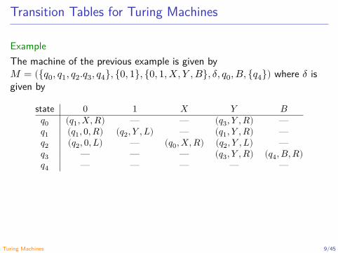
Transition Tables for Turing Machines
ExampleThe machine of the previous example is given by𝑀 = ({𝑞0, 𝑞1, 𝑞2.𝑞3, 𝑞4}, {0, 1}, {0, 1, 𝑋, 𝑌 , 𝐵}, 𝛿, 𝑞0, 𝐵, {𝑞4}) where 𝛿 isgiven by
state 0 1 𝑋 𝑌 𝐵𝑞0 (𝑞1, 𝑋, 𝑅) — — (𝑞3, 𝑌 , 𝑅) —𝑞1 (𝑞1, 0, 𝑅) (𝑞2, 𝑌 , 𝐿) — (𝑞1, 𝑌 , 𝑅) —𝑞2 (𝑞2, 0, 𝐿) — (𝑞0, 𝑋, 𝑅) (𝑞2, 𝑌 , 𝐿) —𝑞3 — — — (𝑞3, 𝑌 , 𝑅) (𝑞4, 𝐵, 𝑅)𝑞4 — — — — —
Turing Machines 9/45
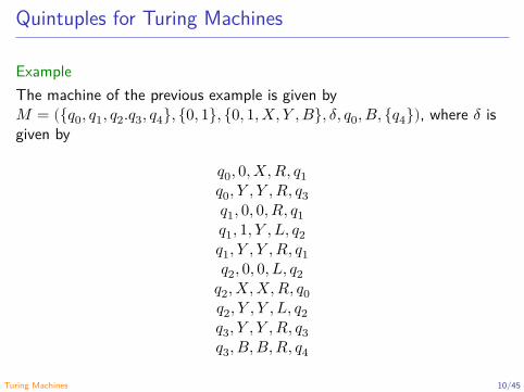
Quintuples for Turing Machines
ExampleThe machine of the previous example is given by𝑀 = ({𝑞0, 𝑞1, 𝑞2.𝑞3, 𝑞4}, {0, 1}, {0, 1, 𝑋, 𝑌 , 𝐵}, 𝛿, 𝑞0, 𝐵, {𝑞4}), where 𝛿 isgiven by
𝑞0, 0, 𝑋, 𝑅, 𝑞1𝑞0, 𝑌 , 𝑌 , 𝑅, 𝑞3𝑞1, 0, 0, 𝑅, 𝑞1𝑞1, 1, 𝑌 , 𝐿, 𝑞2𝑞1, 𝑌 , 𝑌 , 𝑅, 𝑞1𝑞2, 0, 0, 𝐿, 𝑞2
𝑞2, 𝑋, 𝑋, 𝑅, 𝑞0𝑞2, 𝑌 , 𝑌 , 𝐿, 𝑞2𝑞3, 𝑌 , 𝑌 , 𝑅, 𝑞3𝑞3, 𝐵, 𝐵, 𝑅, 𝑞4
Turing Machines 10/45
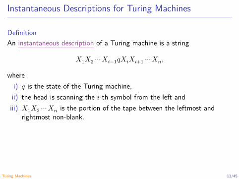
Instantaneous Descriptions for Turing Machines
DefinitionAn instantaneous description of a Turing machine is a string
𝑋1𝑋2 ⋯ 𝑋𝑖−1𝑞𝑋𝑖𝑋𝑖+1 ⋯ 𝑋𝑛,
wherei) 𝑞 is the state of the Turing machine,ii) the head is scanning the 𝑖-th symbol from the left andiii) 𝑋1𝑋2 ⋯ 𝑋𝑛 is the portion of the tape between the leftmost and
rightmost non-blank.
Turing Machines 11/45
Instantaneous Descriptions for Turing Machines
Notation⊢𝑀
: Move of the Turing machine 𝑀 from an instantaneous descriptions toanother.∗⊢𝑀
: Zero o more moves of the Turing machine 𝑀 .
Turing Machines 12/45

Instantaneous Descriptions for Turing Machines
Example0 0 1
𝑞0
𝑋 0 1
𝑞1
𝑋 0 1
𝑞2
𝑞0001 ⊢𝑀
𝑋𝑞101 ⊢𝑀
𝑋0𝑞21
𝑞0001∗⊢𝑀
𝑋0𝑞21
Turing Machines 13/45
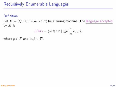
Recursively Enumerable Languages
DefinitionLet 𝑀 = (𝑄, Σ, Γ, 𝛿, 𝑞0, 𝐵, 𝐹) be a Turing machine. The language acceptedby 𝑀 is
𝐿(𝑀) = {𝑤 ∈ Σ∗ ∣ 𝑞0𝑤∗⊢𝑀
𝛼𝑝𝛽},
where 𝑝 ∈ 𝐹 and 𝛼, 𝛽 ∈ Γ∗.
DefinitionA language 𝐿 is recursively enumerable (RE) if exists a Turing machine 𝑀such 𝐿 = 𝐿(𝑀).
Turing Machines 14/45

Recursively Enumerable Languages
DefinitionLet 𝑀 = (𝑄, Σ, Γ, 𝛿, 𝑞0, 𝐵, 𝐹) be a Turing machine. The language acceptedby 𝑀 is
𝐿(𝑀) = {𝑤 ∈ Σ∗ ∣ 𝑞0𝑤∗⊢𝑀
𝛼𝑝𝛽},
where 𝑝 ∈ 𝐹 and 𝛼, 𝛽 ∈ Γ∗.
DefinitionA language 𝐿 is recursively enumerable (RE) if exists a Turing machine 𝑀such 𝐿 = 𝐿(𝑀).
Turing Machines 15/45

Recursively Enumerable Languages
ExampleLet 𝑀 be the machine described by the previous diagram. Then𝐿(𝑀) = {0𝑛1𝑛 ∣ 𝑛 ≥ 1}.See the simulation in the course website.
Turing Machines 16/45

Recursive Languages
ConventionWe assume that a Turing machine halts if it accepts.
What about if the Turing machine does not accept?
RecallRecall that a language 𝐿 is recursively enumerable if exists a Turing ma-chine 𝑀 such that 𝐿 = 𝐿(𝑀).
DefinitionA language 𝐿 is recursive if exists a Turing machine 𝑀 such that
i) 𝐿 = 𝐿(𝑀) andii) 𝑀 always halt (even if it does not accept)
Turing Machines 17/45

Recursive Languages
ConventionWe assume that a Turing machine halts if it accepts.
What about if the Turing machine does not accept?
RecallRecall that a language 𝐿 is recursively enumerable if exists a Turing ma-chine 𝑀 such that 𝐿 = 𝐿(𝑀).
DefinitionA language 𝐿 is recursive if exists a Turing machine 𝑀 such that
i) 𝐿 = 𝐿(𝑀) andii) 𝑀 always halt (even if it does not accept)
Turing Machines 18/45

Recursive Languages
ConventionWe assume that a Turing machine halts if it accepts.
What about if the Turing machine does not accept?
RecallRecall that a language 𝐿 is recursively enumerable if exists a Turing ma-chine 𝑀 such that 𝐿 = 𝐿(𝑀).
DefinitionA language 𝐿 is recursive if exists a Turing machine 𝑀 such that
i) 𝐿 = 𝐿(𝑀) andii) 𝑀 always halt (even if it does not accept)
Turing Machines 19/45

Recursive Languages
ConventionWe assume that a Turing machine halts if it accepts.
What about if the Turing machine does not accept?
RecallRecall that a language 𝐿 is recursively enumerable if exists a Turing ma-chine 𝑀 such that 𝐿 = 𝐿(𝑀).
DefinitionA language 𝐿 is recursive if exists a Turing machine 𝑀 such that
i) 𝐿 = 𝐿(𝑀) andii) 𝑀 always halt (even if it does not accept)
Turing Machines 20/45

Turing Machine Computable Functions
Number-theoretical functionsThe number-theoretical functions are the functions
{𝑓 ∣ 𝑓 ∶ ℕ𝑘 → ℕ}.
ExampleThe following functions are number-theoretical functions:
𝑧(𝑥) = 0 (zero function)𝑠(𝑥) = 𝑥 + 1 (successor function)
𝐼𝑛𝑘 (𝑥1, … , 𝑥𝑛) = 𝑥𝑘 (𝑛-ary projection functions)
𝑖(𝑥) = 𝑥 (identity function)𝑓𝑘(𝑥) = 𝑘 (𝑘-constant function)
𝑥 + 𝑦, 𝑥𝑦, 𝑥𝑦 (addition, multiplication and exponentiation)
Turing Machines 21/45
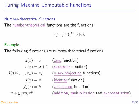
Turing Machine Computable Functions
Number-theoretical functionsThe number-theoretical functions are the functions
{𝑓 ∣ 𝑓 ∶ ℕ𝑘 → ℕ}.
ExampleThe following functions are number-theoretical functions:
𝑧(𝑥) = 0 (zero function)𝑠(𝑥) = 𝑥 + 1 (successor function)
𝐼𝑛𝑘 (𝑥1, … , 𝑥𝑛) = 𝑥𝑘 (𝑛-ary projection functions)
𝑖(𝑥) = 𝑥 (identity function)𝑓𝑘(𝑥) = 𝑘 (𝑘-constant function)
𝑥 + 𝑦, 𝑥𝑦, 𝑥𝑦 (addition, multiplication and exponentiation)
Turing Machines 22/45

Turing Machine Computable Functions
Codification of 𝑘-tuple of natural numbers
�� = 0𝑛 = 0 ⋯ 0⏟𝑛 times
for 𝑛 ∈ ℕ
(𝑛1, 𝑛2, … , 𝑛𝑘) = 𝑛11 𝑛21 ⋯ 1 𝑛𝑘 for (𝑛1, 𝑛2, … , 𝑛𝑘) ∈ ℕ𝑘
Turing Machines 23/45
Turing Machine Computable Functions
DefinitionA function 𝑓 ∶ ℕ → ℕ is Turing machine computable iff exists a machine𝑀 = (𝑄, {0, 1}, Γ, 𝛿, 𝑞0, 𝐵) (there are not accepting states) such that forall 𝑛 ∈ ℕ:From the initial instantaneous description 𝑞0 �� the machine halts with 𝑓(𝑛)on its tape, surrounded by blanks.
RemarkThe definition extends to functions 𝑓 ∶ ℕ𝑘 → ℕ.
Turing Machines 24/45
Turing Machine Computable Functions
DefinitionA function 𝑓 ∶ ℕ → ℕ is Turing machine computable iff exists a machine𝑀 = (𝑄, {0, 1}, Γ, 𝛿, 𝑞0, 𝐵) (there are not accepting states) such that forall 𝑛 ∈ ℕ:From the initial instantaneous description 𝑞0 �� the machine halts with 𝑓(𝑛)on its tape, surrounded by blanks.
RemarkThe definition extends to functions 𝑓 ∶ ℕ𝑘 → ℕ.
Turing Machines 25/45

Turing Machine Computable Functions
ExamplesThe functions𝑧(𝑥) (zero function),𝑠(𝑥) (successor function),𝐼𝑛
𝑘 (𝑥1, … , 𝑥𝑛) (𝑛-ary projection functions),𝑖(𝑥) (identity function),𝑓𝑘(𝑥) (𝑘-constant function),𝑥 + 𝑦, 𝑥𝑦 and 𝑥𝑦
are Turing machine computable functions.
Turing Machines 26/45
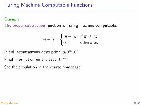
Turing Machine Computable Functions
ExampleThe proper subtraction function is Turing machine computable.
𝑚 ∸ 𝑛 = {𝑚 − 𝑛, if 𝑚 ≥ 𝑛;0, otherwise.
Initial instantaneous description: 𝑞00𝑚10𝑛
Final information on the tape: 0𝑚∸𝑛
See the simulation in the course homepage.
Turing Machines 27/45
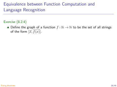
Equivalence between Function Computation andLanguage Recognition
Exercise (8.2.4)Define the graph of a function 𝑓 ∶ ℕ → ℕ to be the set of all stringsof the form [ 𝑥, 𝑓(𝑥)].
A Turing machine is said to compute the function 𝑓 ∶ ℕ → ℕ if,started with 𝑥 on its tape, it halts (in any state) with 𝑓(𝑥) on its tape.
Answer the following, with informal, but clear constructions.
Turing Machines 28/45
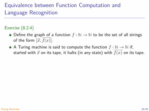
Equivalence between Function Computation andLanguage Recognition
Exercise (8.2.4)Define the graph of a function 𝑓 ∶ ℕ → ℕ to be the set of all stringsof the form [ 𝑥, 𝑓(𝑥)].A Turing machine is said to compute the function 𝑓 ∶ ℕ → ℕ if,started with 𝑥 on its tape, it halts (in any state) with 𝑓(𝑥) on its tape.
Answer the following, with informal, but clear constructions.
Turing Machines 29/45
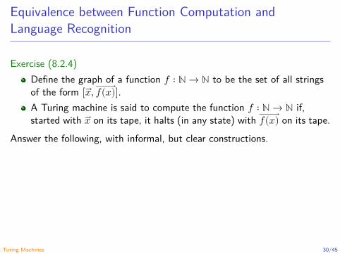
Equivalence between Function Computation andLanguage Recognition
Exercise (8.2.4)Define the graph of a function 𝑓 ∶ ℕ → ℕ to be the set of all stringsof the form [ 𝑥, 𝑓(𝑥)].A Turing machine is said to compute the function 𝑓 ∶ ℕ → ℕ if,started with 𝑥 on its tape, it halts (in any state) with 𝑓(𝑥) on its tape.
Answer the following, with informal, but clear constructions.
Turing Machines 30/45
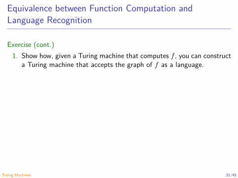
Equivalence between Function Computation andLanguage Recognition
Exercise (cont.)1. Show how, given a Turing machine that computes 𝑓 , you can construct
a Turing machine that accepts the graph of 𝑓 as a language.
2. Show how, given a Turing machine that accepts the graph of 𝑓 , youcan construct a Turing machine that computes 𝑓 .
3. A function is said to partial if it may be undefined for some arguments.If we extend the ideas of this exercise to partial functions, then we donot require that the Turing machine computing 𝑓 halts if its input 𝑥 isone of the natural numbers for which 𝑓(𝑥) is not defined.Do your constructions for parts (1) and (2) work if the function 𝑓 ispartial? If not, explain how you could modify the constructions to makeit work.
Turing Machines 31/45

Equivalence between Function Computation andLanguage Recognition
Exercise (cont.)1. Show how, given a Turing machine that computes 𝑓 , you can construct
a Turing machine that accepts the graph of 𝑓 as a language.2. Show how, given a Turing machine that accepts the graph of 𝑓 , you
can construct a Turing machine that computes 𝑓 .
3. A function is said to partial if it may be undefined for some arguments.If we extend the ideas of this exercise to partial functions, then we donot require that the Turing machine computing 𝑓 halts if its input 𝑥 isone of the natural numbers for which 𝑓(𝑥) is not defined.Do your constructions for parts (1) and (2) work if the function 𝑓 ispartial? If not, explain how you could modify the constructions to makeit work.
Turing Machines 32/45
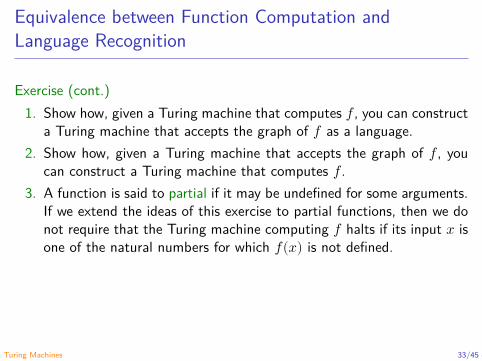
Equivalence between Function Computation andLanguage Recognition
Exercise (cont.)1. Show how, given a Turing machine that computes 𝑓 , you can construct
a Turing machine that accepts the graph of 𝑓 as a language.2. Show how, given a Turing machine that accepts the graph of 𝑓 , you
can construct a Turing machine that computes 𝑓 .3. A function is said to partial if it may be undefined for some arguments.
If we extend the ideas of this exercise to partial functions, then we donot require that the Turing machine computing 𝑓 halts if its input 𝑥 isone of the natural numbers for which 𝑓(𝑥) is not defined.
Do your constructions for parts (1) and (2) work if the function 𝑓 ispartial? If not, explain how you could modify the constructions to makeit work.
Turing Machines 33/45
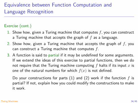
Equivalence between Function Computation andLanguage Recognition
Exercise (cont.)1. Show how, given a Turing machine that computes 𝑓 , you can construct
a Turing machine that accepts the graph of 𝑓 as a language.2. Show how, given a Turing machine that accepts the graph of 𝑓 , you
can construct a Turing machine that computes 𝑓 .3. A function is said to partial if it may be undefined for some arguments.
If we extend the ideas of this exercise to partial functions, then we donot require that the Turing machine computing 𝑓 halts if its input 𝑥 isone of the natural numbers for which 𝑓(𝑥) is not defined.Do your constructions for parts (1) and (2) work if the function 𝑓 ispartial? If not, explain how you could modify the constructions to makeit work.
Turing Machines 34/45

Restrictions to Turing Machines
RestrictionsTuring machines with semi-unbounded tapesMulti-stack machines
TheoremThe previous restrictions are equivalents to Turing machines.
Turing Machines 35/45
Restrictions to Turing Machines
RestrictionsTuring machines with semi-unbounded tapes
Multi-stack machines
TheoremThe previous restrictions are equivalents to Turing machines.
Turing Machines 36/45
Restrictions to Turing Machines
RestrictionsTuring machines with semi-unbounded tapesMulti-stack machines
TheoremThe previous restrictions are equivalents to Turing machines.
Turing Machines 37/45
Restrictions to Turing Machines
RestrictionsTuring machines with semi-unbounded tapesMulti-stack machines
TheoremThe previous restrictions are equivalents to Turing machines.
Turing Machines 38/45
Extensions to Turing Machines
ExtensionsMulti-tape Turing machinesMutil-dimensional tape Turing machinesMulti-head Turing machinesNon-deterministic Turing machinesSubroutines
TheoremThe previous extensions are equivalents to Turing machines.
Turing Machines 39/45

Extensions to Turing Machines
ExtensionsMulti-tape Turing machines
Mutil-dimensional tape Turing machinesMulti-head Turing machinesNon-deterministic Turing machinesSubroutines
TheoremThe previous extensions are equivalents to Turing machines.
Turing Machines 40/45
Extensions to Turing Machines
ExtensionsMulti-tape Turing machinesMutil-dimensional tape Turing machines
Multi-head Turing machinesNon-deterministic Turing machinesSubroutines
TheoremThe previous extensions are equivalents to Turing machines.
Turing Machines 41/45
Extensions to Turing Machines
ExtensionsMulti-tape Turing machinesMutil-dimensional tape Turing machinesMulti-head Turing machines
Non-deterministic Turing machinesSubroutines
TheoremThe previous extensions are equivalents to Turing machines.
Turing Machines 42/45
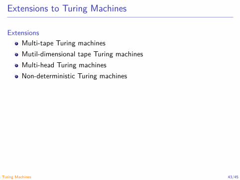
Extensions to Turing Machines
ExtensionsMulti-tape Turing machinesMutil-dimensional tape Turing machinesMulti-head Turing machinesNon-deterministic Turing machines
Subroutines
TheoremThe previous extensions are equivalents to Turing machines.
Turing Machines 43/45

Extensions to Turing Machines
ExtensionsMulti-tape Turing machinesMutil-dimensional tape Turing machinesMulti-head Turing machinesNon-deterministic Turing machinesSubroutines
TheoremThe previous extensions are equivalents to Turing machines.
Turing Machines 44/45
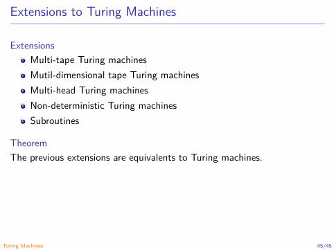
Extensions to Turing Machines
ExtensionsMulti-tape Turing machinesMutil-dimensional tape Turing machinesMulti-head Turing machinesNon-deterministic Turing machinesSubroutines
TheoremThe previous extensions are equivalents to Turing machines.
Turing Machines 45/45

Automata and Formal Languages - CM0081A Language That Is Not Recursively Enumerable
Andrés Sicard-Ramírez
Universidad EAFIT
Semester 2018-1

Undecidability
RecallA language 𝐿 is recursively enumerable if exists a Turing machine 𝑀such that 𝐿 = 𝐿(𝑀).
A language 𝐿 is recursive if exists a Turing machine 𝑀 such thati) 𝐿 = 𝐿(𝑀) andii) 𝑀 always halt (even if it does not accept).
DefinitionA language 𝐿 is undecidable if 𝐿 is not recursive.
A Language That Is Not Recursively Enumerable 2/19
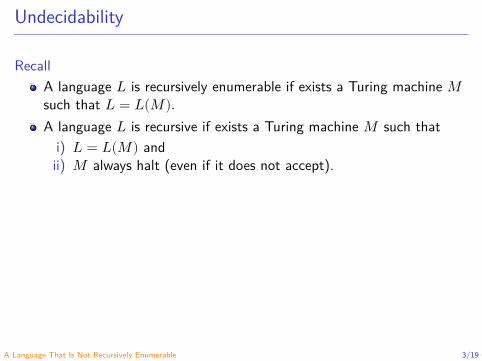
Undecidability
RecallA language 𝐿 is recursively enumerable if exists a Turing machine 𝑀such that 𝐿 = 𝐿(𝑀).A language 𝐿 is recursive if exists a Turing machine 𝑀 such that
i) 𝐿 = 𝐿(𝑀) andii) 𝑀 always halt (even if it does not accept).
DefinitionA language 𝐿 is undecidable if 𝐿 is not recursive.
A Language That Is Not Recursively Enumerable 3/19

Undecidability
RecallA language 𝐿 is recursively enumerable if exists a Turing machine 𝑀such that 𝐿 = 𝐿(𝑀).A language 𝐿 is recursive if exists a Turing machine 𝑀 such that
i) 𝐿 = 𝐿(𝑀) andii) 𝑀 always halt (even if it does not accept).
DefinitionA language 𝐿 is undecidable if 𝐿 is not recursive.
A Language That Is Not Recursively Enumerable 4/19

Why “Recursive”?
The term “recursive” as synonym for “decidable” comes fromMathematics (prior to computers).
Equivalent formalization to Turing-machine computability based onrecursive functions.A function is recursive if only if it is Turing-machine computable (see,for example, (Boolos, Burges and Jeffrey 2007), (Hermes 1969) or(Kleene 1952)).Recursive problem: “it is sufficiently simple that I can write arecursive function to solve it, and the function alwaysfinishes.” (Hopcroft, Motwani and Ullman 2007, p. 385)
A Language That Is Not Recursively Enumerable 5/19
Why “Recursive”?
The term “recursive” as synonym for “decidable” comes fromMathematics (prior to computers).Equivalent formalization to Turing-machine computability based onrecursive functions.
A function is recursive if only if it is Turing-machine computable (see,for example, (Boolos, Burges and Jeffrey 2007), (Hermes 1969) or(Kleene 1952)).Recursive problem: “it is sufficiently simple that I can write arecursive function to solve it, and the function alwaysfinishes.” (Hopcroft, Motwani and Ullman 2007, p. 385)
A Language That Is Not Recursively Enumerable 6/19
Why “Recursive”?
The term “recursive” as synonym for “decidable” comes fromMathematics (prior to computers).Equivalent formalization to Turing-machine computability based onrecursive functions.A function is recursive if only if it is Turing-machine computable (see,for example, (Boolos, Burges and Jeffrey 2007), (Hermes 1969) or(Kleene 1952)).
Recursive problem: “it is sufficiently simple that I can write arecursive function to solve it, and the function alwaysfinishes.” (Hopcroft, Motwani and Ullman 2007, p. 385)
A Language That Is Not Recursively Enumerable 7/19

Why “Recursive”?
The term “recursive” as synonym for “decidable” comes fromMathematics (prior to computers).Equivalent formalization to Turing-machine computability based onrecursive functions.A function is recursive if only if it is Turing-machine computable (see,for example, (Boolos, Burges and Jeffrey 2007), (Hermes 1969) or(Kleene 1952)).Recursive problem: “it is sufficiently simple that I can write arecursive function to solve it, and the function alwaysfinishes.” (Hopcroft, Motwani and Ullman 2007, p. 385)
A Language That Is Not Recursively Enumerable 8/19
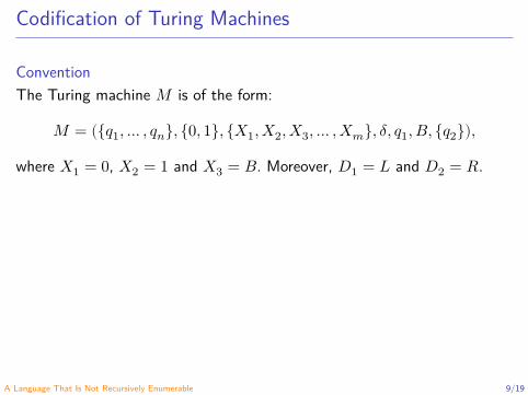
Codification of Turing Machines
ConventionThe Turing machine 𝑀 is of the form:
𝑀 = ({𝑞1, … , 𝑞𝑛}, {0, 1}, {𝑋1, 𝑋2, 𝑋3, … , 𝑋𝑚}, 𝛿, 𝑞1, 𝐵, {𝑞2}),
where 𝑋1 = 0, 𝑋2 = 1 and 𝑋3 = 𝐵. Moreover, 𝐷1 = 𝐿 and 𝐷2 = 𝑅.
Codification of an instructionThe instruction 𝛿(𝑞𝑖, 𝑋𝑗) = (𝑞𝑘, 𝑋𝑙, 𝐷𝑚) is codified by
0𝑖10𝑗10𝑘10𝑙10𝑚.
A Language That Is Not Recursively Enumerable 9/19
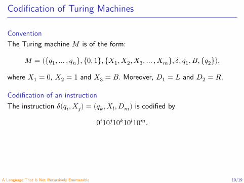
Codification of Turing Machines
ConventionThe Turing machine 𝑀 is of the form:
𝑀 = ({𝑞1, … , 𝑞𝑛}, {0, 1}, {𝑋1, 𝑋2, 𝑋3, … , 𝑋𝑚}, 𝛿, 𝑞1, 𝐵, {𝑞2}),
where 𝑋1 = 0, 𝑋2 = 1 and 𝑋3 = 𝐵. Moreover, 𝐷1 = 𝐿 and 𝐷2 = 𝑅.
Codification of an instructionThe instruction 𝛿(𝑞𝑖, 𝑋𝑗) = (𝑞𝑘, 𝑋𝑙, 𝐷𝑚) is codified by
0𝑖10𝑗10𝑘10𝑙10𝑚.
A Language That Is Not Recursively Enumerable 10/19
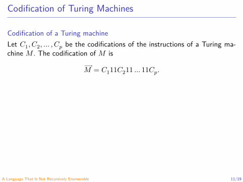
Codification of Turing Machines
Codification of a Turing machineLet 𝐶1, 𝐶2, … , 𝐶𝑝 be the codifications of the instructions of a Turing ma-chine 𝑀 . The codification of 𝑀 is
𝑀 = 𝐶111𝐶211 … 11𝐶𝑝.
RemarkNote that there are other possible codes for 𝑀 .
A Language That Is Not Recursively Enumerable 11/19

Codification of Turing Machines
Codification of a Turing machineLet 𝐶1, 𝐶2, … , 𝐶𝑝 be the codifications of the instructions of a Turing ma-chine 𝑀 . The codification of 𝑀 is
𝑀 = 𝐶111𝐶211 … 11𝐶𝑝.
RemarkNote that there are other possible codes for 𝑀 .
A Language That Is Not Recursively Enumerable 12/19

Codification of Turing Machines
A enumeration for the binary stringsWe ordered the binary strings by [length-]lexicographical order (strings areordered by length, and strings of equal length are ordered lexicographically).If 𝑤 is a binary string, we call 𝑤 the 𝑖-th string where 1𝑤 is the binaryinteger 𝑖. We refer to the 𝑖-th string as 𝑤𝑖.
𝑖-th Turing machineGiven a Turing machine 𝑀 with code 𝑤𝑖, we can now associate a naturalnumber to it: 𝑀 is the 𝑖-th Turing machine, referred to as 𝑀𝑖.
ConventionIf 𝑤𝑖 is not a valid Turing machine code, we shall take 𝑀𝑖 to be the Turingmachine with one state and no transitions. Hence 𝐿(𝑀𝑖) = ∅ if 𝑤𝑖 is not avalid Turing machine code.
A Language That Is Not Recursively Enumerable 13/19

Codification of Turing Machines
A enumeration for the binary stringsWe ordered the binary strings by [length-]lexicographical order (strings areordered by length, and strings of equal length are ordered lexicographically).If 𝑤 is a binary string, we call 𝑤 the 𝑖-th string where 1𝑤 is the binaryinteger 𝑖. We refer to the 𝑖-th string as 𝑤𝑖.
𝑖-th Turing machineGiven a Turing machine 𝑀 with code 𝑤𝑖, we can now associate a naturalnumber to it: 𝑀 is the 𝑖-th Turing machine, referred to as 𝑀𝑖.
ConventionIf 𝑤𝑖 is not a valid Turing machine code, we shall take 𝑀𝑖 to be the Turingmachine with one state and no transitions. Hence 𝐿(𝑀𝑖) = ∅ if 𝑤𝑖 is not avalid Turing machine code.
A Language That Is Not Recursively Enumerable 14/19

Codification of Turing Machines
A enumeration for the binary stringsWe ordered the binary strings by [length-]lexicographical order (strings areordered by length, and strings of equal length are ordered lexicographically).If 𝑤 is a binary string, we call 𝑤 the 𝑖-th string where 1𝑤 is the binaryinteger 𝑖. We refer to the 𝑖-th string as 𝑤𝑖.
𝑖-th Turing machineGiven a Turing machine 𝑀 with code 𝑤𝑖, we can now associate a naturalnumber to it: 𝑀 is the 𝑖-th Turing machine, referred to as 𝑀𝑖.
ConventionIf 𝑤𝑖 is not a valid Turing machine code, we shall take 𝑀𝑖 to be the Turingmachine with one state and no transitions. Hence 𝐿(𝑀𝑖) = ∅ if 𝑤𝑖 is not avalid Turing machine code.
A Language That Is Not Recursively Enumerable 15/19

The Diagonalization Language
The diagonalization languageA language that is not recursively enumerable.
Ld = {𝑤𝑖 ∣ 𝑤𝑖 ∉ 𝐿(𝑀𝑖)}.
𝑤𝑗
𝑀𝑖
1 2 3 4 …1 0 1 1 0 …2 1 1 0 1 …3 0 1 1 0 …4 1 1 0 0 …⋮ ⋮ ⋮ ⋮ ⋮ ⋱
𝑎𝑖𝑗 = {1, if 𝑤𝑗 ∈ 𝐿(𝑀𝑖);0, if 𝑤𝑗 ∉ 𝐿(𝑀𝑖).
Vector for the language 𝐿(𝑀𝑖): 𝑖-th rowLd: Complement of the diagonalIs it possible that Ld be in a row?
A Language That Is Not Recursively Enumerable 16/19

The Diagonalization Language
The diagonalization languageA language that is not recursively enumerable.
Ld = {𝑤𝑖 ∣ 𝑤𝑖 ∉ 𝐿(𝑀𝑖)}.
𝑤𝑗
𝑀𝑖
1 2 3 4 …1 0 1 1 0 …2 1 1 0 1 …3 0 1 1 0 …4 1 1 0 0 …⋮ ⋮ ⋮ ⋮ ⋮ ⋱
𝑎𝑖𝑗 = {1, if 𝑤𝑗 ∈ 𝐿(𝑀𝑖);0, if 𝑤𝑗 ∉ 𝐿(𝑀𝑖).
Vector for the language 𝐿(𝑀𝑖): 𝑖-th rowLd: Complement of the diagonalIs it possible that Ld be in a row?
A Language That Is Not Recursively Enumerable 17/19
The Diagonalization Language
Theorem (9.2)Ld is not recursively enumerable.
ProofWhiteboard.
A Language That Is Not Recursively Enumerable 18/19
References
Boolos, G. S., Burges, J. P. and Jeffrey, R. C. (2007). Computability andLogic. 5th ed. Cambridge University Press (cit. on pp. 5–8).Hermes, H. (1969). Enumerability ⋅ Decidability ⋅ Computability. Secondrevised edition. Springer-Verlag (cit. on pp. 5–8).Hopcroft, J. E., Motwani, R. and Ullman, J. D. (2007). Introduction toAutomata theory, Languages, and Computation. 3rd ed. Pearson Education(cit. on pp. 5–8).Kleene, S. C. (1952). Introduction to Metamathematics. North-Holland(cit. on pp. 5–8).
A Language That Is Not Recursively Enumerable 19/19
Automata and Formal Languages - CM0081An Undecidable Problem That Is Recursively
Enumerable
Andrés Sicard-Ramírez
Universidad EAFIT
Semester 2018-1

Theorems About Recursive Languages
Theorem (9.3)If 𝐿 is a recursive language, so is 𝐿.
ProofWhiteboard.
Theorem (9.4)If both 𝐿 and its complement are recursively enumerable, then 𝐿 is recursive(and by Theorem 9.3, 𝐿 is recursive as well).
ProofWhiteboard.
An Undecidable Problem That Is Recursively Enumerable 2/32
Theorems About Recursive Languages
Theorem (9.3)If 𝐿 is a recursive language, so is 𝐿.
ProofWhiteboard.
Theorem (9.4)If both 𝐿 and its complement are recursively enumerable, then 𝐿 is recursive(and by Theorem 9.3, 𝐿 is recursive as well).
ProofWhiteboard.
An Undecidable Problem That Is Recursively Enumerable 3/32
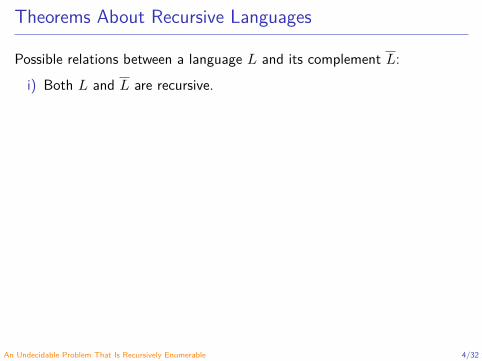
Theorems About Recursive Languages
Possible relations between a language 𝐿 and its complement 𝐿:i) Both 𝐿 and 𝐿 are recursive.
ii) Neither 𝐿 nor 𝐿 are recursively enumerable.iii) 𝐿 is recursively enumerable but not recursive and 𝐿 is not recursively
enumerable.iv) 𝐿 is recursively enumerable but not recursive and 𝐿 is not recursively
enumerable.
An Undecidable Problem That Is Recursively Enumerable 4/32
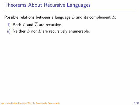
Theorems About Recursive Languages
Possible relations between a language 𝐿 and its complement 𝐿:i) Both 𝐿 and 𝐿 are recursive.ii) Neither 𝐿 nor 𝐿 are recursively enumerable.
iii) 𝐿 is recursively enumerable but not recursive and 𝐿 is not recursivelyenumerable.
iv) 𝐿 is recursively enumerable but not recursive and 𝐿 is not recursivelyenumerable.
An Undecidable Problem That Is Recursively Enumerable 5/32

Theorems About Recursive Languages
Possible relations between a language 𝐿 and its complement 𝐿:i) Both 𝐿 and 𝐿 are recursive.ii) Neither 𝐿 nor 𝐿 are recursively enumerable.iii) 𝐿 is recursively enumerable but not recursive and 𝐿 is not recursively
enumerable.
iv) 𝐿 is recursively enumerable but not recursive and 𝐿 is not recursivelyenumerable.
An Undecidable Problem That Is Recursively Enumerable 6/32
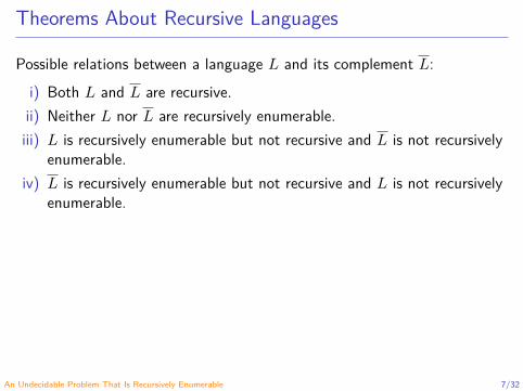
Theorems About Recursive Languages
Possible relations between a language 𝐿 and its complement 𝐿:i) Both 𝐿 and 𝐿 are recursive.ii) Neither 𝐿 nor 𝐿 are recursively enumerable.iii) 𝐿 is recursively enumerable but not recursive and 𝐿 is not recursively
enumerable.iv) 𝐿 is recursively enumerable but not recursive and 𝐿 is not recursively
enumerable.
An Undecidable Problem That Is Recursively Enumerable 7/32

Theorems About Recursive Languages
Exercise (9.2.5)Let 𝐿 be recursively enumerable and let 𝐿 be non-RE. Consider thelanguage
𝐿′ = {0𝑤 ∣ 𝑤 is in 𝐿} ∪ {1𝑤 ∣ 𝑤 is not in 𝐿}.Can you say for certain whether 𝐿′ is recursive, RE, or non-RE? Justifyyour answer.
Solution (from Hopcroft, Motwani and Ullman (2007))Suppose 𝐿′ were RE. Then we could design a Turing machine 𝑀 for 𝐿as follows. Given input 𝑤, 𝑀 changes its input to 1𝑤 and simulates thehypothetical Turing machine for 𝐿′. If that Turing machine accepts, then 𝑤is in 𝐿, so 𝑀 should accept. If the Turing machine for 𝐿′ never accepts,then neither does 𝑀 . Thus, 𝑀 would accept exactly 𝐿, which contradictsthe fact that 𝐿 is not RE. We conclude that 𝐿′ is not RE.
An Undecidable Problem That Is Recursively Enumerable 8/32
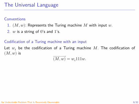
The Universal Language
Conventions1. (𝑀, 𝑤): Represents the Turing machine 𝑀 with input 𝑤.2. 𝑤 is a string of 0’s and 1’s.
Codification of a Turing machine with an inputLet 𝑤𝑖 be the codification of a Turing machine 𝑀 . The codification of(𝑀, 𝑤) is
(𝑀, 𝑤) = 𝑤𝑖111𝑤.
An Undecidable Problem That Is Recursively Enumerable 9/32
The Universal Language
The universal language Lu
An undecidable language that is recursively enumerable.
The set of binary strings that encode a pair (𝑀, 𝑤) such that 𝑤 ∈ 𝐿(𝑀),
Lu = { (𝑀, 𝑤) ∣ 𝑤 ∈ 𝐿(𝑀)} .TheoremLu is recursively enumerable.
Idea of the proofExists a Turing machine U such that Lu = 𝐿(U). The machine U is calleda universal Turing machine.
An Undecidable Problem That Is Recursively Enumerable 10/32
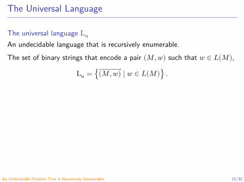
The Universal Language
The universal language Lu
An undecidable language that is recursively enumerable.The set of binary strings that encode a pair (𝑀, 𝑤) such that 𝑤 ∈ 𝐿(𝑀),
Lu = { (𝑀, 𝑤) ∣ 𝑤 ∈ 𝐿(𝑀)} .
TheoremLu is recursively enumerable.
Idea of the proofExists a Turing machine U such that Lu = 𝐿(U). The machine U is calleda universal Turing machine.
An Undecidable Problem That Is Recursively Enumerable 11/32
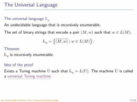
The Universal Language
The universal language Lu
An undecidable language that is recursively enumerable.The set of binary strings that encode a pair (𝑀, 𝑤) such that 𝑤 ∈ 𝐿(𝑀),
Lu = { (𝑀, 𝑤) ∣ 𝑤 ∈ 𝐿(𝑀)} .TheoremLu is recursively enumerable.
Idea of the proofExists a Turing machine U such that Lu = 𝐿(U). The machine U is calleda universal Turing machine.
An Undecidable Problem That Is Recursively Enumerable 12/32
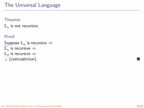
The Universal Language
TheoremLu is not recursive.
Proof.Suppose Lu is recursive ⇒Lu is recursive ⇒Ld is recursive ⇒⊥ (contradiction).
An Undecidable Problem That Is Recursively Enumerable 13/32

Code for a Universal Turing Machine
Since 𝑈 is a Turing machine exists 𝑖 (1654 digits) such that 𝑈 = 𝑀𝑖 givenby (using a different codification) (Penrose 1991, pp. 56-57):7244855335339317577198395039615711237952360672556559631108144796606505059404241090310483613632359365644443458382226883278767626556144692814117715017842551707554085657689753346356942478488597046934725739988582283827795294683460521061169835945938791885546326440925525505820555989451890716537414896033096753020431553625034984529832320651583047664142130708819329717234151056980262734686429921838172157333482823073453713421475059740345184372359593090640024321077342178851492760797597634415123079586396354492269159479654614711345700145048167337562172573464522731054482980784965126988788964569760906634204477989021914437932830019493570963921703904833270882596201301773727202718625919914428275437422351355675134084222299889374410534305471044368695876405178128019437530813870639942772823156425289237514565443899052780793241144826142357286193118332610656122755531810207511085337633806031082361675045635852164214869542347187426437544428790062485827091240422076538754264454133451748566291574299909502623009733738137724162172747723610206786854002893566085696822620141982486216989026091309402985706001743006700868967590344734174127874255812015493663938996905817738591654055356704092821332221631410978710814599786695997045096818419062994436560151454904880922084480034822492077304030431884298993931352668823496621019471619107014619685231928474820344958977095535611070275817487333272966789987984732840981907648512726310017401667873634776058572450369644348979920344899974556624029374876688397514044516657077500605138839916688140725455446652220507242623923792115253181625125363050931728631422004064571305275802307665183351995689139748137504926429605010013651980186945639498
An Undecidable Problem That Is Recursively Enumerable 14/32

The Original Universal Turing Machine
Based on 𝑀 -functions (subroutines with parameters) (Sicard 1997;Copeland 2004b).The machine is composed by 12 symbols and 4.000 instructions,approximately (Sicard Ramírez 1998).
An Undecidable Problem That Is Recursively Enumerable 15/32
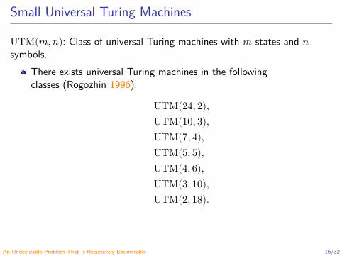
Small Universal Turing Machines
UTM(𝑚, 𝑛): Class of universal Turing machines with 𝑚 states and 𝑛symbols.
There exists universal Turing machines in the followingclasses (Rogozhin 1996):
UTM(24, 2),UTM(10, 3),UTM(7, 4),UTM(5, 5),UTM(4, 6),UTM(3, 10),UTM(2, 18).
The classes UTM(3, 2), UTM(2, 3) and UTM(2, 2) areempty (Rogozhin 1996).
An Undecidable Problem That Is Recursively Enumerable 16/32

Small Universal Turing Machines
UTM(𝑚, 𝑛): Class of universal Turing machines with 𝑚 states and 𝑛symbols.
There exists universal Turing machines in the followingclasses (Rogozhin 1996):
UTM(24, 2),UTM(10, 3),UTM(7, 4),UTM(5, 5),UTM(4, 6),UTM(3, 10),UTM(2, 18).
The classes UTM(3, 2), UTM(2, 3) and UTM(2, 2) areempty (Rogozhin 1996).
An Undecidable Problem That Is Recursively Enumerable 17/32

Wolfram Turing MachineTHE BOOK STORE DOWNLOADS EDUCATION ARCHIVES FORUM
© 2012 Stephen Wolfram, LLC stephenwolfram.com | wolfram.com | send a message | contact info
Announced May 14th, 2007: 5th Anniversary of the Publication of A New Kindof Science
Is this Turing machine universal, ornot?
The machine has 2 states and 3 colors, and is 596440 in Wolfram's numbering scheme.
If it is universal then it is the smallest universal Turing machine that exists.
BACKGROUND » TECHNICAL DETAILS » GALLERY » NEWS »
PRIZE COMMITTEE » RULES & GUIDELINES » FAQs »
A universal Turing machine is powerful enough to emulate any standard computer.
The question is: how simple can the rules for a universal Turing machine be?
Since the 1960s it has been known that there is a universal 7,4 machine. In A New
Kind of Science, Stephen Wolfram found a universal 2,5 machine, and suggested that
the particular 2,3 machine that is the subject of this prize might be universal.
The prize is for determining whether or not the 2,3 machine is in fact universal.
What is a Turing Machine? » | Notable Universal Turing Machines »
INTERACTIVE DEMONSTRATIONS » PRINTABLE POSTER »
NKS|ONLINE »
SPONSORED BY WOLFRAM RESEARCH & STEPHEN WOLFRAM
Wolfram 2,3 Turing Machine Research Prize http://www.wolframscience.com/prizes/tm23/
1 of 1 10/11/2012 09:31 AM
An Undecidable Problem That Is Recursively Enumerable 18/32

Conway’s Game of Life
From: WikipediaNote: Adobe Reader is required to see the simulation (tested with AdobeReader 9.9.5 on Ubuntu).
ExamplesPulsar (Oscillator)Author: Jokey Smurf
Glider (Spaceship)Author: Rodrigo Silveira Camargo
An Undecidable Problem That Is Recursively Enumerable 19/32
Conway’s Game of Life
Rulesi) Any live cell with fewer than two live neighbours dies, as if caused by
under-population.
ii) Any live cell with two or three live neighbours lives on to the nextgeneration.
iii) Any live cell with more than three live neighbours dies, as if byovercrowding.
iv) Any dead cell with exactly three live neighbours becomes a live cell,as if by reproduction.
TheoremIt is possible codified a universal Turing machine in Conway’s Game ofLife (Rendell 2011).
An Undecidable Problem That Is Recursively Enumerable 20/32

Conway’s Game of Life
Rulesi) Any live cell with fewer than two live neighbours dies, as if caused by
under-population.ii) Any live cell with two or three live neighbours lives on to the next
generation.
iii) Any live cell with more than three live neighbours dies, as if byovercrowding.
iv) Any dead cell with exactly three live neighbours becomes a live cell,as if by reproduction.
TheoremIt is possible codified a universal Turing machine in Conway’s Game ofLife (Rendell 2011).
An Undecidable Problem That Is Recursively Enumerable 21/32

Conway’s Game of Life
Rulesi) Any live cell with fewer than two live neighbours dies, as if caused by
under-population.ii) Any live cell with two or three live neighbours lives on to the next
generation.iii) Any live cell with more than three live neighbours dies, as if by
overcrowding.
iv) Any dead cell with exactly three live neighbours becomes a live cell,as if by reproduction.
TheoremIt is possible codified a universal Turing machine in Conway’s Game ofLife (Rendell 2011).
An Undecidable Problem That Is Recursively Enumerable 22/32
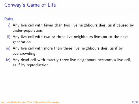
Conway’s Game of Life
Rulesi) Any live cell with fewer than two live neighbours dies, as if caused by
under-population.ii) Any live cell with two or three live neighbours lives on to the next
generation.iii) Any live cell with more than three live neighbours dies, as if by
overcrowding.iv) Any dead cell with exactly three live neighbours becomes a live cell,
as if by reproduction.
TheoremIt is possible codified a universal Turing machine in Conway’s Game ofLife (Rendell 2011).
An Undecidable Problem That Is Recursively Enumerable 23/32
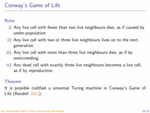
Conway’s Game of Life
Rulesi) Any live cell with fewer than two live neighbours dies, as if caused by
under-population.ii) Any live cell with two or three live neighbours lives on to the next
generation.iii) Any live cell with more than three live neighbours dies, as if by
overcrowding.iv) Any dead cell with exactly three live neighbours becomes a live cell,
as if by reproduction.
TheoremIt is possible codified a universal Turing machine in Conway’s Game ofLife (Rendell 2011).
An Undecidable Problem That Is Recursively Enumerable 24/32

The Halting Problem
The original Turing machine accepted by halting, no by final state.
H(𝑀) = {𝑤 ∣ 𝑀 halts given the input 𝑤}.
The halting problem (language)
Lhp = { (𝑀, 𝑤) ∣ 𝑤 ∈ H(𝑀)} .
Example (Exercise 9.2.1)Show that Lhp is recursively enumerable but not recursive.
An Undecidable Problem That Is Recursively Enumerable 25/32
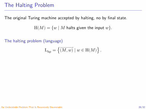
The Halting Problem
The original Turing machine accepted by halting, no by final state.
H(𝑀) = {𝑤 ∣ 𝑀 halts given the input 𝑤}.
The halting problem (language)
Lhp = { (𝑀, 𝑤) ∣ 𝑤 ∈ H(𝑀)} .
Example (Exercise 9.2.1)Show that Lhp is recursively enumerable but not recursive.
An Undecidable Problem That Is Recursively Enumerable 26/32

The Halting Problem
The original Turing machine accepted by halting, no by final state.
H(𝑀) = {𝑤 ∣ 𝑀 halts given the input 𝑤}.
The halting problem (language)
Lhp = { (𝑀, 𝑤) ∣ 𝑤 ∈ H(𝑀)} .
Example (Exercise 9.2.1)Show that Lhp is recursively enumerable but not recursive.
An Undecidable Problem That Is Recursively Enumerable 27/32
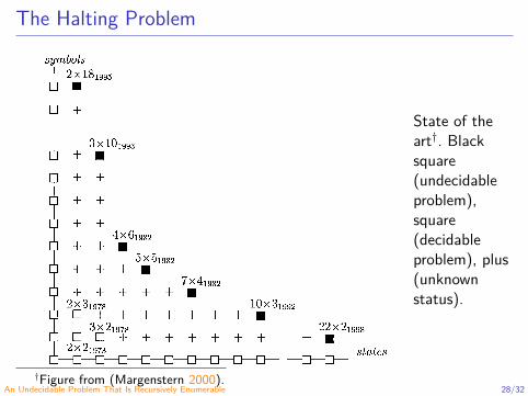
The Halting Problem230 M. Margenstern / Theoretical Computer Science 231 (2000) 217–251
Fig. 2. The state of the art. Black squares indicate undecidable points, while squares indicate decidablepoints, points marked with plus between the white squares lines and the line of black squares in the shapeof a hyperbola correspond to sets for which the status of the halting problem is not known.
author improved some of the results obtained in 1982 [94–96]. Yet his paper of 1982had remained unnoticed by the scienti�c community for ten years. The technique usedin order to obtain these results will be explained in our survey, in Section 3.4.2.Let us have a look now in the opposite direction: it is trivial that Turing machines on
a single letter alphabet have a decidable halting problem. It is not that trivial that thesame property holds for machines with a single state, whatever the number of symbolsis in the machine alphabet. This was de�nitely proved by Hermann in 1966 [32].For more than one state, one does not know much. As for proving the decidability
of the halting problem, M. Minsky writes in his famous book of 1967 that he andone of his students “did this for all 2× 2 machines [1961, unpublished] by a tediousreduction to thirty-odd cases (unpublishable)” [72, p. 281, last two lines]. Six yearslater, Pavlotskaya proved the same theorem [82] in a compact, very short proof. Thispaper has also remained unnoticed for many years. A few years later [84], she provedthat the point 3× 2 is also decidable.All these results about the decidability and undecidability of the halting problem for
Turing machines can be represented as in Fig. 2.
3.1. Decidability criteria
Let us now introduce a more precise notion of decidability criterion, respectivelystrong decidability criterion. Let c be an integer-valued function de�ned on a set Mof Turing machines in M with the following property: there is an integer f such that
State of theart†. Blacksquare(undecidableproblem),square(decidableproblem), plus(unknownstatus).
†Figure from (Margenstern 2000).An Undecidable Problem That Is Recursively Enumerable 28/32
The Halting Problem
RemarkThe halting problem was introduced and named by Davis (1958, p. 70.)not by Turing himself, contrary to popular belief (Copeland 2004a, p. 40).
Practical approach“In contrast to popular belief, proving termination is not always im-possible.” (Cook, Podelski and Rybalchenko 2011, p. 1)
An Undecidable Problem That Is Recursively Enumerable 29/32
The Halting Problem
RemarkThe halting problem was introduced and named by Davis (1958, p. 70.)not by Turing himself, contrary to popular belief (Copeland 2004a, p. 40).
Practical approach“In contrast to popular belief, proving termination is not always im-possible.” (Cook, Podelski and Rybalchenko 2011, p. 1)
An Undecidable Problem That Is Recursively Enumerable 30/32

References
Cook, B., Podelski, A. and Rybalchenko, A. (2011). Proving ProgramTermination. Communications of the ACM 54.5, pp. 88–98. doi:10.1145/1941487.1941509 (cit. on pp. 29, 30).Copeland, B. J. (2004a). Hypercomputation: Philosophical Issues.Theoretical Computer Science 317.1–3, pp. 251–267. doi:10.1016/j.tcs.2003.12.014 (cit. on pp. 29, 30).Davis, M. (1958). Computability and Unsolvability. McGraw-Hill (cit. onpp. 29, 30).Hopcroft, J. E., Motwani, R. and Ullman, J. D. (2007). Introduction toAutomata theory, Languages, and Computation. 3rd ed. Pearson Education(cit. on p. 8).Margenstern, M. (2000). Frontier Between Decidability and Undecidability:A Survey. Theoretical Computer Science 231.2, pp. 217–251. doi:10.1016/S0304-3975(99)00102-4 (cit. on p. 28).Penrose, R. (1991). The Emperor’s New Mind. Penguin Books (cit. onp. 14).
An Undecidable Problem That Is Recursively Enumerable 31/32
References
Rendell, P. (2011). A Universal Turing Machine in Conway’s Game of Life.In: Proceedings of the 2011 International Conference on High PerformanceComputing & Simulation (HPCS 2011). Ed. by Smari, W. W. IEEE,pp. 764–772. doi: 10.1109/HPCSim.2011.5999906 (cit. on pp. 20–24).Rogozhin, Y. (1996). Small Universal Turing Machines. TheoreticalComputer Science 168, pp. 215–240. doi: 10.1016/S0304-3975(96)00077-1(cit. on pp. 16, 17).Sicard Ramírez, A. (1998). Máquinas de Turing Dinámicas: Historia yDesarrollo de una Idea. MA thesis. Departamento de Informática ySistemas. Universidad EAFIT (cit. on p. 15).Sicard, A. (1997). Máquina Universal de Turing: Algunas Indicaciones parasu Construcción. Rev. U. EAFIT 33.108, pp. 61–106 (cit. on p. 15).Sicard, A. and Copeland, B. J. (2004b). Appendix: Subroutines andM-functions. In: The Essential Turing. Vol. 317. 1–3, pp. 54–57. doi:10.1016/j.tcs.2003.12.014 (cit. on p. 15).
An Undecidable Problem That Is Recursively Enumerable 32/32
Automata and Formal Languages - CM0081Undecidable Problems About Turing Machines
Andrés Sicard-Ramírez
Universidad EAFIT
Semester 2018-1

Reductions
DefinitionLet 𝑃1 and 𝑃2 be two problems. A reduction from 𝑃1 to 𝑃2 is a Turingmachine that takes an instance of 𝑃1 written on its tape and halts with aninstance of 𝑃2 that have the same answer (i.e. a reduction is an algorithm).
yes
no
yes
no
𝑃1 𝑃2
Undecidable Problems About Turing Machines 2/28

Reductions
Theorem (9.7.a)If there is a reduction from 𝑃1 to 𝑃2 then if 𝑃1 is undecidable then so 𝑃2.(Hint: Suppose the 𝑃2 is decidable and find a contradiction).
Theorem (9.7.b)If there is a reduction from 𝑃1 to 𝑃2 then if 𝑃1 is not recursively enumerablethen so 𝑃2. (Hint: Suppose the 𝑃2 is recursively enumerable and find acontradiction).
Undecidable Problems About Turing Machines 3/28
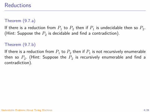
Reductions
Theorem (9.7.a)If there is a reduction from 𝑃1 to 𝑃2 then if 𝑃1 is undecidable then so 𝑃2.(Hint: Suppose the 𝑃2 is decidable and find a contradiction).
Theorem (9.7.b)If there is a reduction from 𝑃1 to 𝑃2 then if 𝑃1 is not recursively enumerablethen so 𝑃2. (Hint: Suppose the 𝑃2 is recursively enumerable and find acontradiction).
Undecidable Problems About Turing Machines 4/28
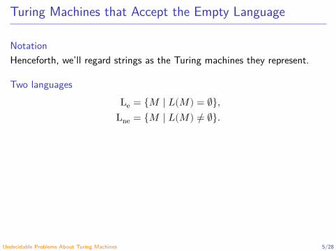
Turing Machines that Accept the Empty Language
NotationHenceforth, we’ll regard strings as the Turing machines they represent.
Two languagesLe = {𝑀 ∣ 𝐿(𝑀) = ∅},
Lne = {𝑀 ∣ 𝐿(𝑀) ≠ ∅}.
Undecidable Problems About Turing Machines 5/28

Turing Machines that Accept the Empty Language
Theorem (9.8)Lne is recursively enumerable.
ProofConstruction of a non-determinist Turing machine to accept Lne:†
†Figure from Hopcroft, Motwani and Ullman (2007, Fig. 9.8).Undecidable Problems About Turing Machines 6/28
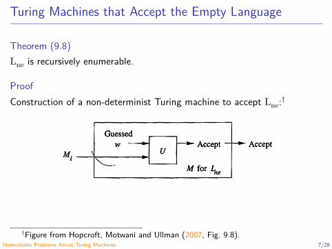
Turing Machines that Accept the Empty Language
Theorem (9.8)Lne is recursively enumerable.
ProofConstruction of a non-determinist Turing machine to accept Lne:†
†Figure from Hopcroft, Motwani and Ullman (2007, Fig. 9.8).Undecidable Problems About Turing Machines 7/28

Turing Machines that Accept the Empty Language
Theorem (9.9)Lne is not recursive.
Undecidable Problems About Turing Machines 8/28
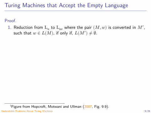
Turing Machines that Accept the Empty Language
Proof.1. Reduction from Lu to Lne where the pair (𝑀, 𝑤) is converted in 𝑀 ′,
such that 𝑤 ∈ 𝐿(𝑀), if only if, 𝐿(𝑀 ′) ≠ ∅.
2. The key is to have 𝑀 ′ ignore its input.†
3. Lne is not recursive by Theorem 9.7.a.
†Figure from Hopcroft, Motwani and Ullman (2007, Fig. 9.9).Undecidable Problems About Turing Machines 9/28

Turing Machines that Accept the Empty Language
Proof.1. Reduction from Lu to Lne where the pair (𝑀, 𝑤) is converted in 𝑀 ′,
such that 𝑤 ∈ 𝐿(𝑀), if only if, 𝐿(𝑀 ′) ≠ ∅.2. The key is to have 𝑀 ′ ignore its input.†
3. Lne is not recursive by Theorem 9.7.a.
†Figure from Hopcroft, Motwani and Ullman (2007, Fig. 9.9).Undecidable Problems About Turing Machines 10/28
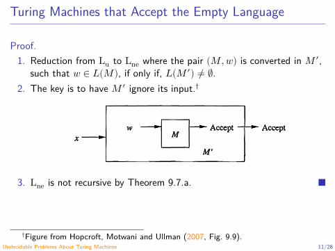
Turing Machines that Accept the Empty Language
Proof.1. Reduction from Lu to Lne where the pair (𝑀, 𝑤) is converted in 𝑀 ′,
such that 𝑤 ∈ 𝐿(𝑀), if only if, 𝐿(𝑀 ′) ≠ ∅.2. The key is to have 𝑀 ′ ignore its input.†
3. Lne is not recursive by Theorem 9.7.a.
†Figure from Hopcroft, Motwani and Ullman (2007, Fig. 9.9).Undecidable Problems About Turing Machines 11/28
Turing Machines that Accept the Empty Language
Theorem (9.10)Le is not recursively enumerable. (Hint: Le is the complement of Lne).
Undecidable Problems About Turing Machines 12/28

Rice’s Theorem
Set of the recursively enumerable languages
ℒ = {𝐿 ∣ 𝐿 is a recursively enumerable language }.
Properties (subsets) of the recursively enumerable languagesProperty 𝑃 of ℒ: 𝑃 ⊆ ℒ.
Example (Trivial properties)𝑃 (𝐿) = ∅ or 𝑃(𝐿) = ℒ.
Example𝑃 (𝐿): 𝐿 is a language regular.
Undecidable Problems About Turing Machines 13/28
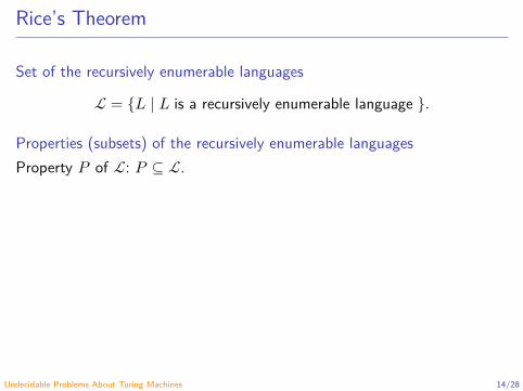
Rice’s Theorem
Set of the recursively enumerable languages
ℒ = {𝐿 ∣ 𝐿 is a recursively enumerable language }.
Properties (subsets) of the recursively enumerable languagesProperty 𝑃 of ℒ: 𝑃 ⊆ ℒ.
Example (Trivial properties)𝑃 (𝐿) = ∅ or 𝑃(𝐿) = ℒ.
Example𝑃 (𝐿): 𝐿 is a language regular.
Undecidable Problems About Turing Machines 14/28
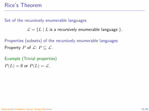
Rice’s Theorem
Set of the recursively enumerable languages
ℒ = {𝐿 ∣ 𝐿 is a recursively enumerable language }.
Properties (subsets) of the recursively enumerable languagesProperty 𝑃 of ℒ: 𝑃 ⊆ ℒ.
Example (Trivial properties)𝑃 (𝐿) = ∅ or 𝑃(𝐿) = ℒ.
Example𝑃 (𝐿): 𝐿 is a language regular.
Undecidable Problems About Turing Machines 15/28
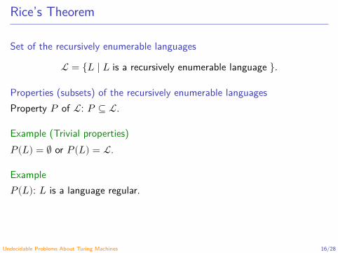
Rice’s Theorem
Set of the recursively enumerable languages
ℒ = {𝐿 ∣ 𝐿 is a recursively enumerable language }.
Properties (subsets) of the recursively enumerable languagesProperty 𝑃 of ℒ: 𝑃 ⊆ ℒ.
Example (Trivial properties)𝑃 (𝐿) = ∅ or 𝑃(𝐿) = ℒ.
Example𝑃 (𝐿): 𝐿 is a language regular.
Undecidable Problems About Turing Machines 16/28
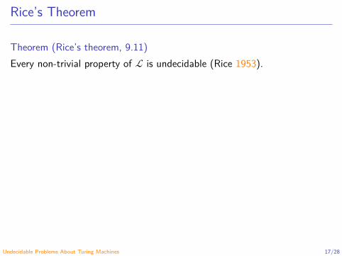
Rice’s Theorem
Theorem (Rice’s theorem, 9.11)Every non-trivial property of ℒ is undecidable (Rice 1953).
How to prove Rice’s theorem?We identify a property 𝑃 by the Turing machines 𝑀 such that 𝐿(𝑀) ∈ 𝑃 .
Theorem (Rice’s theorem (second version))If 𝑃 ⊆ ℒ is a non-trivial property then
𝐿𝑃 = {𝑀 ∣ 𝐿(𝑀) ∈ 𝑃}
is undecidable.
Undecidable Problems About Turing Machines 17/28

Rice’s Theorem
Theorem (Rice’s theorem, 9.11)Every non-trivial property of ℒ is undecidable (Rice 1953).
How to prove Rice’s theorem?We identify a property 𝑃 by the Turing machines 𝑀 such that 𝐿(𝑀) ∈ 𝑃 .
Theorem (Rice’s theorem (second version))If 𝑃 ⊆ ℒ is a non-trivial property then
𝐿𝑃 = {𝑀 ∣ 𝐿(𝑀) ∈ 𝑃}
is undecidable.
Undecidable Problems About Turing Machines 18/28

Rice’s Theorem
Theorem (Rice’s theorem, 9.11)Every non-trivial property of ℒ is undecidable (Rice 1953).
How to prove Rice’s theorem?We identify a property 𝑃 by the Turing machines 𝑀 such that 𝐿(𝑀) ∈ 𝑃 .
Theorem (Rice’s theorem (second version))If 𝑃 ⊆ ℒ is a non-trivial property then
𝐿𝑃 = {𝑀 ∣ 𝐿(𝑀) ∈ 𝑃}
is undecidable.
Undecidable Problems About Turing Machines 19/28

Rice’s Theorem
Proof: Case ∅ ∉ 𝑃 .1. Let 𝐿 be a language and 𝑀𝐿 be a Turing machine such 𝐿 ≠ ∅,
𝐿 ∈ 𝑃 and 𝐿 = 𝐿(𝑀𝐿). Reduction from Lu to 𝐿𝑃 where the pair(𝑀, 𝑤) is converted in 𝑀 ′ such that:†
i) 𝐿(𝑀 ′) = ∅ (i.e. 𝑀 ′ ∉ 𝐿𝑃 ) if 𝑤 ∉ 𝐿(𝑀) andii) 𝐿(𝑀 ′) = 𝐿 (i.e. 𝑀 ′ ∈ 𝐿𝑃 ) if 𝑤 ∈ 𝐿(𝑀).
2. 𝐿𝑃 is not recursive by Theorem 9.7.a.
†Figure from Hopcroft, Motwani and Ullman (2007, Fig. 9.10).Undecidable Problems About Turing Machines 20/28

Rice’s Theorem
Proof: Case ∅ ∉ 𝑃 .1. Let 𝐿 be a language and 𝑀𝐿 be a Turing machine such 𝐿 ≠ ∅,
𝐿 ∈ 𝑃 and 𝐿 = 𝐿(𝑀𝐿). Reduction from Lu to 𝐿𝑃 where the pair(𝑀, 𝑤) is converted in 𝑀 ′ such that:†
i) 𝐿(𝑀 ′) = ∅ (i.e. 𝑀 ′ ∉ 𝐿𝑃 ) if 𝑤 ∉ 𝐿(𝑀) andii) 𝐿(𝑀 ′) = 𝐿 (i.e. 𝑀 ′ ∈ 𝐿𝑃 ) if 𝑤 ∈ 𝐿(𝑀).
2. 𝐿𝑃 is not recursive by Theorem 9.7.a.
†Figure from Hopcroft, Motwani and Ullman (2007, Fig. 9.10).Undecidable Problems About Turing Machines 21/28
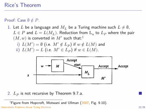
Rice’s Theorem
Proof: Case ∅ ∉ 𝑃 .1. Let 𝐿 be a language and 𝑀𝐿 be a Turing machine such 𝐿 ≠ ∅,
𝐿 ∈ 𝑃 and 𝐿 = 𝐿(𝑀𝐿). Reduction from Lu to 𝐿𝑃 where the pair(𝑀, 𝑤) is converted in 𝑀 ′ such that:†
i) 𝐿(𝑀 ′) = ∅ (i.e. 𝑀 ′ ∉ 𝐿𝑃 ) if 𝑤 ∉ 𝐿(𝑀) andii) 𝐿(𝑀 ′) = 𝐿 (i.e. 𝑀 ′ ∈ 𝐿𝑃 ) if 𝑤 ∈ 𝐿(𝑀).
2. 𝐿𝑃 is not recursive by Theorem 9.7.a.†Figure from Hopcroft, Motwani and Ullman (2007, Fig. 9.10).
Undecidable Problems About Turing Machines 22/28

Rice’s Theorem
Proof: Case ∅ ∈ 𝑃 .1. By the previous case, 𝑃 is undecidable, i.e. 𝐿𝑃 is undecidable.2. 𝐿𝑃 = 𝐿𝑃 .3. Suppose 𝐿𝑃 is decidable then 𝐿𝑃 would be also decidable
(contradiction).4. Therefore, 𝐿𝑃 is undecidable.
Undecidable Problems About Turing Machines 23/28

Rice’s Theorem
All the problems about Turing machines that involve only the language thatthe Turing machine accepts are undecidable.
ExamplesIs the language accepted by the Turing machine empty? Is it finite? Isit regular? Is it context-free?Does the language accepted by the Turing machine contain the string“hello world”? Does it contain all the even numbers?
Undecidable Problems About Turing Machines 24/28

Rice’s Theorem
All the problems about Turing machines that involve only the language thatthe Turing machine accepts are undecidable.
ExamplesIs the language accepted by the Turing machine empty? Is it finite? Isit regular? Is it context-free?Does the language accepted by the Turing machine contain the string“hello world”? Does it contain all the even numbers?
Undecidable Problems About Turing Machines 25/28
Rice’s Theorem
Rice’s theorem does not imply that everything about Turing machines isundecidable.
ExampleIt is decidable if a Turing machine has five states.
Undecidable Problems About Turing Machines 26/28
Rice’s Theorem
Rice’s theorem does not imply that everything about Turing machines isundecidable.ExampleIt is decidable if a Turing machine has five states.
Undecidable Problems About Turing Machines 27/28
References
Hopcroft, J. E., Motwani, R. and Ullman, J. D. (2007). Introduction toAutomata theory, Languages, and Computation. 3rd ed. Pearson Education(cit. on pp. 6, 7, 9–11, 20–22).Rice, H. G. (1953). Classes of Recursively Enumerable Sets and TheirDecision Problems. Trans. Amer. Math. Soc. 74.2, pp. 358–366. doi:10.1090/S0002-9947-1953-0053041-6 (cit. on pp. 17–19).
Undecidable Problems About Turing Machines 28/28

Automata and Formal Languages - CM0081Undecidable Problems
Andrés Sicard-Ramírez
Universidad EAFIT
Semester 2018-1

Undecidable Problems
(From Wikipedia)Problems in logicProblems about abstract machinesProblems about matricesProblems in combinatorial group theoryProblems in topologyProblems in analysis…
Undecidable Problems 2/21

Normal Forms for the 𝜆-Calculus
RemarkThis problem was the first undecidable problem. See (Church 1935).
DefinitionThe set of 𝜆-terms, denoted by Λ, is inductively defined by:
𝑥 ∈ 𝑉 ⇒ 𝑥 ∈ Λ (variable)𝑀, 𝑁 ∈ Λ ⇒ (𝑀𝑁) ∈ Λ (application)
𝑀 ∈ Λ, 𝑥 ∈ 𝑉 ⇒ (𝜆𝑥𝑀) ∈ Λ (abstraction)
where 𝑉 is a set of variables.
Undecidable Problems 3/21
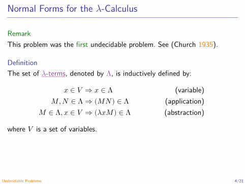
Normal Forms for the 𝜆-Calculus
RemarkThis problem was the first undecidable problem. See (Church 1935).
DefinitionThe set of 𝜆-terms, denoted by Λ, is inductively defined by:
𝑥 ∈ 𝑉 ⇒ 𝑥 ∈ Λ (variable)𝑀, 𝑁 ∈ Λ ⇒ (𝑀𝑁) ∈ Λ (application)
𝑀 ∈ Λ, 𝑥 ∈ 𝑉 ⇒ (𝜆𝑥𝑀) ∈ Λ (abstraction)
where 𝑉 is a set of variables.
Undecidable Problems 4/21

Normal Forms for the 𝜆-Calculus
DefinitionThe 𝛽-reduction is defined by
(𝜆𝑥𝑀)𝑁 →𝛽 𝑀[𝑥 ∶= 𝑁],
where 𝑀[𝑥 ∶= 𝑁] denotes the substitution of 𝑁 for the free occurrencesof 𝑥 in 𝑀 .
Examples(𝜆𝑦.𝑦𝑦)𝑥 →𝛽 𝑥𝑥
(𝜆𝑥.(𝜆𝑦.𝑦𝑥)𝑧)𝑣 →𝛽 (𝜆𝑦.𝑦𝑣)𝑧 →𝛽 𝑧𝑣
Let Ω be (𝜆𝑥.𝑥𝑥)(𝜆𝑥.𝑥𝑥), then Ω →𝛽 Ω →𝛽 ⋯
Undecidable Problems 5/21
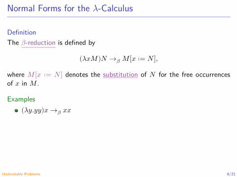
Normal Forms for the 𝜆-Calculus
DefinitionThe 𝛽-reduction is defined by
(𝜆𝑥𝑀)𝑁 →𝛽 𝑀[𝑥 ∶= 𝑁],
where 𝑀[𝑥 ∶= 𝑁] denotes the substitution of 𝑁 for the free occurrencesof 𝑥 in 𝑀 .
Examples(𝜆𝑦.𝑦𝑦)𝑥 →𝛽 𝑥𝑥
(𝜆𝑥.(𝜆𝑦.𝑦𝑥)𝑧)𝑣 →𝛽 (𝜆𝑦.𝑦𝑣)𝑧 →𝛽 𝑧𝑣
Let Ω be (𝜆𝑥.𝑥𝑥)(𝜆𝑥.𝑥𝑥), then Ω →𝛽 Ω →𝛽 ⋯
Undecidable Problems 6/21
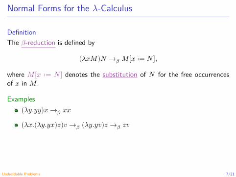
Normal Forms for the 𝜆-Calculus
DefinitionThe 𝛽-reduction is defined by
(𝜆𝑥𝑀)𝑁 →𝛽 𝑀[𝑥 ∶= 𝑁],
where 𝑀[𝑥 ∶= 𝑁] denotes the substitution of 𝑁 for the free occurrencesof 𝑥 in 𝑀 .
Examples(𝜆𝑦.𝑦𝑦)𝑥 →𝛽 𝑥𝑥
(𝜆𝑥.(𝜆𝑦.𝑦𝑥)𝑧)𝑣 →𝛽 (𝜆𝑦.𝑦𝑣)𝑧 →𝛽 𝑧𝑣
Let Ω be (𝜆𝑥.𝑥𝑥)(𝜆𝑥.𝑥𝑥), then Ω →𝛽 Ω →𝛽 ⋯
Undecidable Problems 7/21
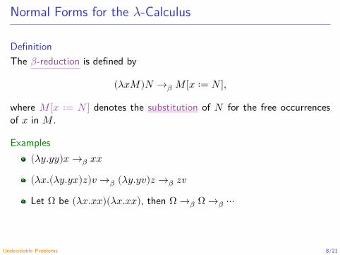
Normal Forms for the 𝜆-Calculus
DefinitionThe 𝛽-reduction is defined by
(𝜆𝑥𝑀)𝑁 →𝛽 𝑀[𝑥 ∶= 𝑁],
where 𝑀[𝑥 ∶= 𝑁] denotes the substitution of 𝑁 for the free occurrencesof 𝑥 in 𝑀 .
Examples(𝜆𝑦.𝑦𝑦)𝑥 →𝛽 𝑥𝑥
(𝜆𝑥.(𝜆𝑦.𝑦𝑥)𝑧)𝑣 →𝛽 (𝜆𝑦.𝑦𝑣)𝑧 →𝛽 𝑧𝑣
Let Ω be (𝜆𝑥.𝑥𝑥)(𝜆𝑥.𝑥𝑥), then Ω →𝛽 Ω →𝛽 ⋯
Undecidable Problems 8/21
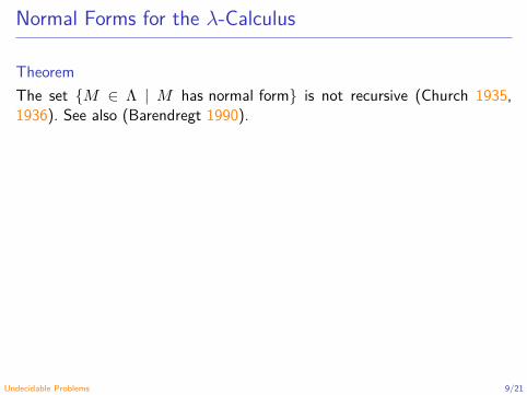
Normal Forms for the 𝜆-Calculus
TheoremThe set {𝑀 ∈ Λ ∣ 𝑀 has normal form} is not recursive (Church 1935,1936). See also (Barendregt 1990).
Undecidable Problems 9/21

Post’s Correspondence Problem (PCP)
An instance of the PCPAn instance of PCP consist of two lists of equal length 𝐴 = 𝑤1, … , 𝑤𝑘 and𝐵 = 𝑥1, … , 𝑥𝑘 of strings over an alphabet Σ. We say this instance of PCPhas a solution, if there is a sequence of one or more integers 𝑖1, … , 𝑖𝑚, with𝑚 ≥ 1 that, when interpreted as indexes for strings in the 𝐴 and 𝐵 lists,yield the same string, i.e. 𝑤𝑖1
⋯ 𝑤𝑖𝑚= 𝑥𝑖1
⋯ 𝑥𝑖𝑚. The sequence 𝑖1, … , 𝑖𝑚
is called a solution of the instance of PCP.
The problemGiven an instance of PCP, tell whether this instance has a solution.
Undecidable Problems 10/21

Post’s Correspondence Problem (PCP)
An instance of the PCPAn instance of PCP consist of two lists of equal length 𝐴 = 𝑤1, … , 𝑤𝑘 and𝐵 = 𝑥1, … , 𝑥𝑘 of strings over an alphabet Σ. We say this instance of PCPhas a solution, if there is a sequence of one or more integers 𝑖1, … , 𝑖𝑚, with𝑚 ≥ 1 that, when interpreted as indexes for strings in the 𝐴 and 𝐵 lists,yield the same string, i.e. 𝑤𝑖1
⋯ 𝑤𝑖𝑚= 𝑥𝑖1
⋯ 𝑥𝑖𝑚. The sequence 𝑖1, … , 𝑖𝑚
is called a solution of the instance of PCP.
The problemGiven an instance of PCP, tell whether this instance has a solution.
Undecidable Problems 11/21
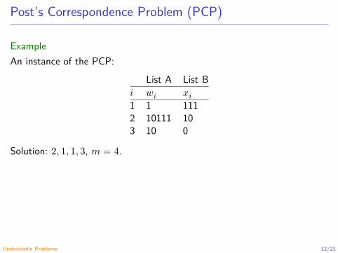
Post’s Correspondence Problem (PCP)
ExampleAn instance of the PCP:
List A List B𝑖 𝑤𝑖 𝑥𝑖1 1 1112 10111 103 10 0
Solution: 2, 1, 1, 3, 𝑚 = 4.
Undecidability proofThe PCP problem is undecidable (Post 1946). Hopcroft, Motwani and Ull-man (2007) shows the undecidability via a reduction of Lu to PCP.
Undecidable Problems 12/21

Post’s Correspondence Problem (PCP)
ExampleAn instance of the PCP:
List A List B𝑖 𝑤𝑖 𝑥𝑖1 1 1112 10111 103 10 0
Solution: 2, 1, 1, 3, 𝑚 = 4.
Undecidability proofThe PCP problem is undecidable (Post 1946). Hopcroft, Motwani and Ull-man (2007) shows the undecidability via a reduction of Lu to PCP.
Undecidable Problems 13/21

The Mortal Matrix Problem (MMP)
The problemLet 𝑆 be a finite set of 𝑛 × 𝑛 matrices with integer entries. To determinewhether the zero matrix belongs to the semigroup generated by 𝑆, i.e.to determine whether the matrices in 𝑆 can be multiplied in some order,possibly with repetitions, to yield the zero matrix.
Some undecidable instancesThe MMP is undecidable for a set of seven 3 × 3 matrices, or a set of two21 × 21 matrices (Halava, Harju and Hirvensalo 2007).
Undecidability proofReduction of PCP to MMP.
Undecidable Problems 14/21

The Mortal Matrix Problem (MMP)
The problemLet 𝑆 be a finite set of 𝑛 × 𝑛 matrices with integer entries. To determinewhether the zero matrix belongs to the semigroup generated by 𝑆, i.e.to determine whether the matrices in 𝑆 can be multiplied in some order,possibly with repetitions, to yield the zero matrix.
Some undecidable instancesThe MMP is undecidable for a set of seven 3 × 3 matrices, or a set of two21 × 21 matrices (Halava, Harju and Hirvensalo 2007).
Undecidability proofReduction of PCP to MMP.
Undecidable Problems 15/21

The Mortal Matrix Problem (MMP)
The problemLet 𝑆 be a finite set of 𝑛 × 𝑛 matrices with integer entries. To determinewhether the zero matrix belongs to the semigroup generated by 𝑆, i.e.to determine whether the matrices in 𝑆 can be multiplied in some order,possibly with repetitions, to yield the zero matrix.
Some undecidable instancesThe MMP is undecidable for a set of seven 3 × 3 matrices, or a set of two21 × 21 matrices (Halava, Harju and Hirvensalo 2007).
Undecidability proofReduction of PCP to MMP.
Undecidable Problems 16/21

Hilbert’s Tenth Problem (HTP)
DefinitionA Diophantine equation is an equation of the form
𝐷(𝑥1, … , 𝑥𝑘) = 0,
where 𝐷 is a polynomial with integer coefficients.
The problem (in present terminology)“Given a Diophantine equation with any number of unknowns: To devise aprocess according to which it can be determined by a finite number of op-erations whether the equation has non-negative integer solutions.” (Sicard,Ospina and Vélez 2006, p. 12542)
Undecidability proofA set is recursively enumerable if and only if it is Diophantine (Matiyasevich1993).
Undecidable Problems 17/21
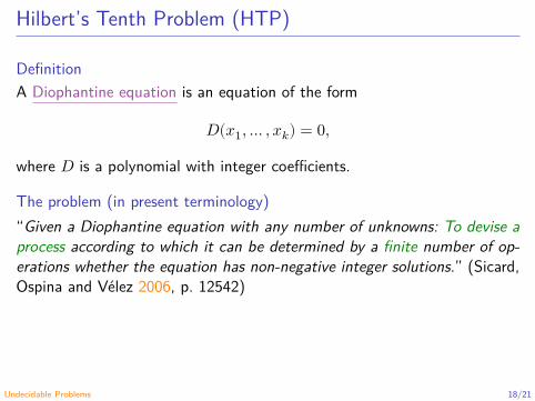
Hilbert’s Tenth Problem (HTP)
DefinitionA Diophantine equation is an equation of the form
𝐷(𝑥1, … , 𝑥𝑘) = 0,
where 𝐷 is a polynomial with integer coefficients.
The problem (in present terminology)“Given a Diophantine equation with any number of unknowns: To devise aprocess according to which it can be determined by a finite number of op-erations whether the equation has non-negative integer solutions.” (Sicard,Ospina and Vélez 2006, p. 12542)
Undecidability proofA set is recursively enumerable if and only if it is Diophantine (Matiyasevich1993).
Undecidable Problems 18/21
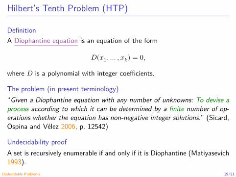
Hilbert’s Tenth Problem (HTP)
DefinitionA Diophantine equation is an equation of the form
𝐷(𝑥1, … , 𝑥𝑘) = 0,
where 𝐷 is a polynomial with integer coefficients.
The problem (in present terminology)“Given a Diophantine equation with any number of unknowns: To devise aprocess according to which it can be determined by a finite number of op-erations whether the equation has non-negative integer solutions.” (Sicard,Ospina and Vélez 2006, p. 12542)
Undecidability proofA set is recursively enumerable if and only if it is Diophantine (Matiyasevich1993).
Undecidable Problems 19/21

References
Barendregt, H. (1990). Functional Programming and Lambda Calculus. In:Handbook of Theoretical Computer Science. Ed. by van Leeuwen, J. Vol. B.Formal Models and Semantics. MIT Press. Chap. 7. doi:10.1016/B978-0-444-88074-1.50012-3 (cit. on p. 9).Church, A. (1935). An Unsolvable Problem of Elementary Number Theory.Preliminar Report (Abstract). Bull. Amer. Math. Soc. 41.5, pp. 332–333.doi: 10.1090/S0002-9904-1935-06102-6 (cit. on pp. 3, 4, 9).— (1936). An Unsolvable Problem of Elementary Number Theory.American Journal of Mathematics 58.2, pp. 345–363. doi:10.2307/2371045 (cit. on p. 9).Halava, V., Harju, T. and Hirvensalo, M. (2007). Undecidability Bounds forInteger Matrices Using Claus Instances. International Journal ofFoundations of Computer Science 18.5, pp. 931–948. doi:10.1142/S0129054107005066 (cit. on pp. 14–16).
Undecidable Problems 20/21
References
Hopcroft, J. E., Motwani, R. and Ullman, J. D. (2007). Introduction toAutomata theory, Languages, and Computation. 3rd ed. Pearson Education(cit. on pp. 12, 13).Matiyasevich, Y. V. (1993). Hilbert’s Tenth Problem. MIT Press (cit. onpp. 17–19).Post, E. (1946). A Variant of a Recursively Unsolvable Problem. Bull.Amer. Math. Soc. 52, pp. 264–268. doi:10.1090/S0002-9904-1946-08555-9 (cit. on pp. 12, 13).Sicard, A., Ospina, J. and Vélez, M. (2006). Quantum HypercomputationBased on the Dynamical Algebra 𝔰𝔲(1, 1). J. Phys. A: Math. Gen. 39.40,pp. 12539–12558. doi: 10.1088/0305-4470/39/40/018 (cit. on pp. 17–19).
Undecidable Problems 21/21
Automata and Formal Languages - CM0081The Church-Turing Thesis
Andrés Sicard-Ramírez
Universidad EAFIT
Semester 2018-1
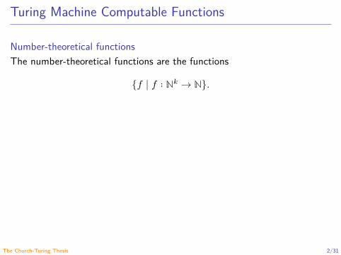
Turing Machine Computable Functions
Number-theoretical functionsThe number-theoretical functions are the functions
{𝑓 ∣ 𝑓 ∶ ℕ𝑘 → ℕ}.
ExampleThe following functions are Turing machine computable:
𝑧(𝑥) = 0 (zero function)𝑠(𝑥) = 𝑥 + 1 (successor function)
𝐼𝑛𝑘 (𝑥1, … , 𝑥𝑛) = 𝑥𝑘 (𝑛-ary projection functions)
𝑖(𝑥) = 𝑥 (identity function)𝑓𝑘(𝑥) = 𝑘 (𝑘-constant function)
𝑥 + 𝑦, 𝑥𝑦, 𝑥𝑦 (addition, multiplication and exponentiation)
The Church-Turing Thesis 2/31

Turing Machine Computable Functions
Number-theoretical functionsThe number-theoretical functions are the functions
{𝑓 ∣ 𝑓 ∶ ℕ𝑘 → ℕ}.
ExampleThe following functions are Turing machine computable:
𝑧(𝑥) = 0 (zero function)𝑠(𝑥) = 𝑥 + 1 (successor function)
𝐼𝑛𝑘 (𝑥1, … , 𝑥𝑛) = 𝑥𝑘 (𝑛-ary projection functions)
𝑖(𝑥) = 𝑥 (identity function)𝑓𝑘(𝑥) = 𝑘 (𝑘-constant function)
𝑥 + 𝑦, 𝑥𝑦, 𝑥𝑦 (addition, multiplication and exponentiation)
The Church-Turing Thesis 3/31
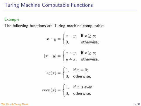
Turing Machine Computable Functions
ExampleThe following functions are Turing machine computable:
𝑥 ∸ 𝑦 = {𝑥 − 𝑦, if 𝑥 ≥ 𝑦;0, otherwise;
|𝑥 − 𝑦| = {𝑥 ∸ 𝑦, if 𝑥 ≥ 𝑦;𝑦 ∸ 𝑥, otherwise;
𝑠𝑔(𝑥) = {1, if 𝑥 = 0;0, otherwise;
𝑒𝑣𝑒𝑛(𝑥) = {1, if 𝑥 is even;0, otherwise.
The Church-Turing Thesis 4/31

Common Versions of the Church-Turing Thesis
“A function is computable (effectively calculable) if and only if there is aTuring machine which computes it.” (Galton 2006, p. 94)
“The unprovable assumption that any general way to compute will allowus compute only the partial-recursive functions (or equivalently, what Tur-ing machines or modern-day computers can compute) is know as Church’shypothesis or the Church-Turing thesis.” (Hopcroft, Motwani and Ullman2007, p. 236)
The Church-Turing Thesis 5/31

Common Versions of the Church-Turing Thesis
“A function is computable (effectively calculable) if and only if there is aTuring machine which computes it.” (Galton 2006, p. 94)“The unprovable assumption that any general way to compute will allowus compute only the partial-recursive functions (or equivalently, what Tur-ing machines or modern-day computers can compute) is know as Church’shypothesis or the Church-Turing thesis.” (Hopcroft, Motwani and Ullman2007, p. 236)
The Church-Turing Thesis 6/31

Alonzo Church: A Definition
“We now define the notion, already discussed,of an effectively calculable function of posit-ive integers by identifying it with the notion ofa recursive function of positive integers (or ofa 𝜆-definable function of positive integers).This definition is thought to be justified byconsiderations which follow, so far as positivejustification can ever be obtained for the se-lection of a formal definition to correspond tointuitive notion.” (Church 1936, p. 356)See also (Church 1935).
The Church-Turing Thesis 7/31

Alan Turing: A Definition
“The ‘computable’ numbers† include all num-bers which would naturally be regarded ascomputable.” (Turing 1936, p. 249)
†The number whose decimal representation can be generating progressively by aTuring machine.
The Church-Turing Thesis 8/31

Stephen Kleene: Church’s thesis and Turing’s thesis
“The thesis of Church and Turing werenot even called ‘thesis’ at all until Kleene(1943, p. 60)† referred to Church’s ‘defin-ition’ as ‘Thesis I’ and the 1952 Kleene‡
referred to ‘Church’s Thesis’ and ‘Turing’sThesis’.” (Soare 1996, pp. 295–296)
†Kleene, S. C. (1943). Recursive Predicates and Quantifiers.‡Kleene, S. C. (1952). Introduction to Metamathematics.
The Church-Turing Thesis 9/31

Stephen Kleene: The Church-Turing Thesis
“The term ‘Church-Turing thesis’ seems to have been first introduce byKleene, with a small flourish of bias in favor of Church:” (Copeland 2002)
“So Turing’s and Church’s thesis are equival-ent. We shall usually refer to them both asChurch’s thesis, or in connection with that one ofits…version which deal with ‘Turing machines’ asthe Church-Turing thesis.” (Kleene 1967, p. 232)
The Church-Turing Thesis 10/31
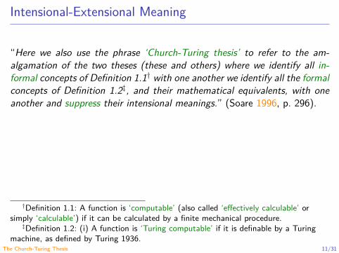
Intensional-Extensional Meaning
“Here we also use the phrase ‘Church-Turing thesis’ to refer to the am-algamation of the two theses (these and others) where we identify all in-formal concepts of Definition 1.1† with one another we identify all the formalconcepts of Definition 1.2‡, and their mathematical equivalents, with oneanother and suppress their intensional meanings.” (Soare 1996, p. 296).
†Definition 1.1: A function is ‘computable’ (also called ‘effectively calculable’ orsimply ‘calculable’) if it can be calculated by a finite mechanical procedure.
‡Definition 1.2: (i) A function is ‘Turing computable’ if it is definable by a Turingmachine, as defined by Turing 1936.
The Church-Turing Thesis 11/31
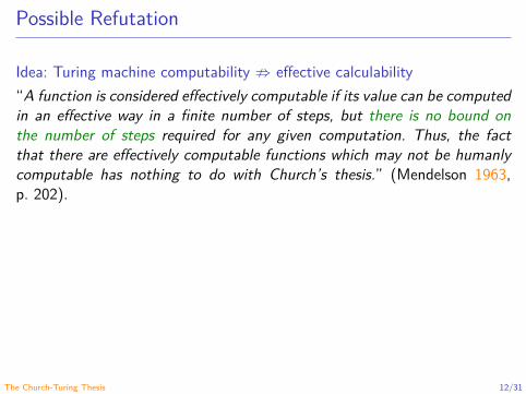
Possible Refutation
Idea: Turing machine computability ⇏ effective calculability“A function is considered effectively computable if its value can be computedin an effective way in a finite number of steps, but there is no bound onthe number of steps required for any given computation. Thus, the factthat there are effectively computable functions which may not be humanlycomputable has nothing to do with Church’s thesis.” (Mendelson 1963,p. 202).
The Church-Turing Thesis 12/31

Possible Refutation
Idea: Effective calculability ⇏ Turing machine computability(the interesting one!)
From a Church’s letter to Pepis (June 8, 1937):“Therefore to discover a function which was effectively calculable but nogeneral recursive would imply discovery of an utterly new principle of logic,not only never before formulated, but never before actually used in a math-ematical proof…Moreover this new principle of logic must be of so strange,and presumably complicated,…I should be inclined to scrutinize the allegedeffective applicability of the principle with considerable care.” (Sieg 1997,pp. 175–176)
The Church-Turing Thesis 13/31

A Precise Version of the Church-Turing Thesis
Turing’ analysis: Features of computations performed by human computers
“States of mind” ⇒ Finite number of states
A human cannot reliably discriminate infinitely many symbols ⇒Finite alphabet
Unlimited sheets of paper ⇒ Unbounded tape
The human read/write symbols on the paper ⇒ Read/Write head
Human’s shift of attention form one part of the paper to another ⇒Displacement of the read/write head
The Church-Turing Thesis 14/31
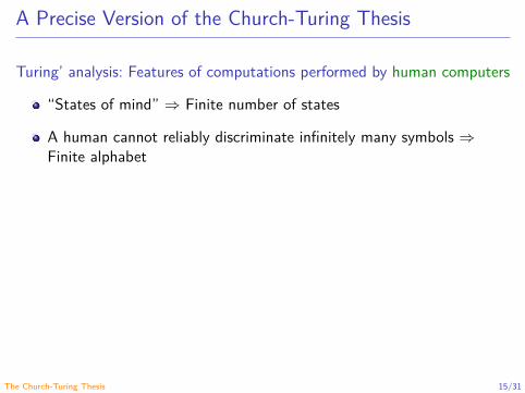
A Precise Version of the Church-Turing Thesis
Turing’ analysis: Features of computations performed by human computers
“States of mind” ⇒ Finite number of states
A human cannot reliably discriminate infinitely many symbols ⇒Finite alphabet
Unlimited sheets of paper ⇒ Unbounded tape
The human read/write symbols on the paper ⇒ Read/Write head
Human’s shift of attention form one part of the paper to another ⇒Displacement of the read/write head
The Church-Turing Thesis 15/31
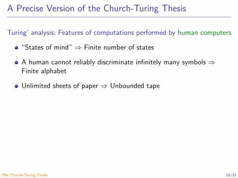
A Precise Version of the Church-Turing Thesis
Turing’ analysis: Features of computations performed by human computers
“States of mind” ⇒ Finite number of states
A human cannot reliably discriminate infinitely many symbols ⇒Finite alphabet
Unlimited sheets of paper ⇒ Unbounded tape
The human read/write symbols on the paper ⇒ Read/Write head
Human’s shift of attention form one part of the paper to another ⇒Displacement of the read/write head
The Church-Turing Thesis 16/31
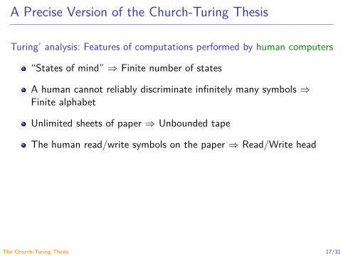
A Precise Version of the Church-Turing Thesis
Turing’ analysis: Features of computations performed by human computers
“States of mind” ⇒ Finite number of states
A human cannot reliably discriminate infinitely many symbols ⇒Finite alphabet
Unlimited sheets of paper ⇒ Unbounded tape
The human read/write symbols on the paper ⇒ Read/Write head
Human’s shift of attention form one part of the paper to another ⇒Displacement of the read/write head
The Church-Turing Thesis 17/31

A Precise Version of the Church-Turing Thesis
Turing’ analysis: Features of computations performed by human computers
“States of mind” ⇒ Finite number of states
A human cannot reliably discriminate infinitely many symbols ⇒Finite alphabet
Unlimited sheets of paper ⇒ Unbounded tape
The human read/write symbols on the paper ⇒ Read/Write head
Human’s shift of attention form one part of the paper to another ⇒Displacement of the read/write head
The Church-Turing Thesis 18/31
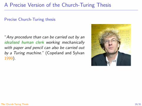
A Precise Version of the Church-Turing Thesis
Precise Church-Turing thesis
“Any procedure than can be carried out by anidealised human clerk working mechanicallywith paper and pencil can also be carried outby a Turing machine.” (Copeland and Sylvan1999).
The Church-Turing Thesis 19/31

Other Theses
Gandy’s theses (Gandy n.d.)
“Thesis P. A discrete deterministicmechanical device satisfies prin-ciples I-IV below.” (p. 126)
“Theorem. What can be calculatedby a device satisfying principles I-IVis computable.” (p. 126)
“Thesis M. What can be calculatedby a machine is Turing machinecomputable.” (p. 124)
The Church-Turing Thesis 20/31

Other Theses
Gandy’s theses (Gandy n.d.)
“Thesis P. A discrete deterministicmechanical device satisfies prin-ciples I-IV below.” (p. 126)
“Theorem. What can be calculatedby a device satisfying principles I-IVis computable.” (p. 126)
“Thesis M. What can be calculatedby a machine is Turing machinecomputable.” (p. 124)
The Church-Turing Thesis 21/31
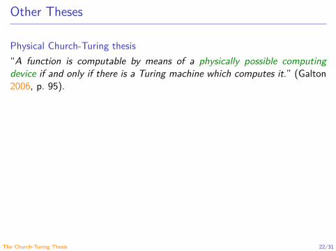
Other Theses
Physical Church-Turing thesis“A function is computable by means of a physically possible computingdevice if and only if there is a Turing machine which computes it.” (Galton2006, p. 95).
The Church-Turing Thesis 22/31

Current Situation
At the moment, it does not exists a refutation to the preciseChurch-Turing thesis.
The hypercomputation models refute the theoretical version of thethesis M.
Open problem: the refutation of the realizable version of the thesis M(i.e. the physical Church-Turing thesis).
The Church-Turing Thesis 23/31
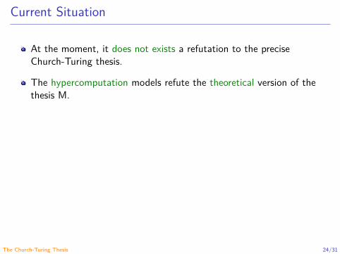
Current Situation
At the moment, it does not exists a refutation to the preciseChurch-Turing thesis.
The hypercomputation models refute the theoretical version of thethesis M.
Open problem: the refutation of the realizable version of the thesis M(i.e. the physical Church-Turing thesis).
The Church-Turing Thesis 24/31

Current Situation
At the moment, it does not exists a refutation to the preciseChurch-Turing thesis.
The hypercomputation models refute the theoretical version of thethesis M.
Open problem: the refutation of the realizable version of the thesis M(i.e. the physical Church-Turing thesis).
The Church-Turing Thesis 25/31

Bonus Slides: Higher Type Computability
ExampleLet 𝑓 and ⊥ be a terminating and a non-terminating function from 𝑎 to 𝑎,respectively. The parallel or function
por ∷ (𝑎 → 𝑎) → (𝑎 → 𝑎) → 𝑎 → 𝑎por 𝑓 ⊥ = 𝑓por ⊥ 𝑓 = 𝑓por ⊥ ⊥ = ⊥
is an effectively calculable function which is not 𝜆-definable (Turner 2006).
The Church-Turing Thesis 26/31

Bonus Slides: Higher Type Computability
Solution: To add extra primitives to 𝜆-calculus (interleaving, concurrency,etc.).
General problem: A definition of higher type computability (see, forexample, (Longley 2003)).
The Church-Turing Thesis 27/31
Bonus Slides: Higher Type Computability
Solution: To add extra primitives to 𝜆-calculus (interleaving, concurrency,etc.).General problem: A definition of higher type computability (see, forexample, (Longley 2003)).
The Church-Turing Thesis 28/31

References
Church, A. (1935). An Unsolvable Problem of Elementary Number Theory.Preliminar Report (Abstract). Bull. Amer. Math. Soc. 41.5, pp. 332–333.doi: 10.1090/S0002-9904-1935-06102-6 (cit. on p. 7).— (1936). An Unsolvable Problem of Elementary Number Theory.American Journal of Mathematics 58.2, pp. 345–363. doi:10.2307/2371045 (cit. on p. 7).Copeland, B. J. (19th Aug. 2002). The Church-Turing Thesis. StanfordEncyclopedia of Philosophy (cit. on p. 10).Copeland, B. J. and Sylvan, R. (1999). Beyond the Universal TuringMachine. Australasian Journal of Philosophy 77.1, pp. 44–66. doi:10.1080/00048409912348801 (cit. on p. 19).Galton, A. (2006). The Church-Turing Thesis: Still Valid after All TheseYears? Applied Mathematics and Computation 178.1, pp. 93–102. doi:10.1016/j.amc.2005.09.086 (cit. on pp. 5, 6, 22).
The Church-Turing Thesis 29/31
References
Gandy, R. (n.d.). Church’s Thesis and Principles for Mechanisms. In: TheKleene Symposium, pp. 123–148. doi: 10.1016/S0049-237X(08)71257-6(cit. on pp. 20, 21).Hopcroft, J. E., Motwani, R. and Ullman, J. D. (2007). Introduction toAutomata theory, Languages, and Computation. 3rd ed. Pearson Education(cit. on pp. 5, 6).Kleene, S. C. (1943). Recursive Predicates and Quantifiers. Trans. Amer.Math. Soc. 53.1, pp. 41–73. doi: 10.1090/S0002-9947-1943-0007371-8(cit. on p. 9).Kleene, S. C. (1952). Introduction to Metamathematics. North-Holland(cit. on p. 9).— (1967). Mathematical Logic. John Wiley & Sons (cit. on p. 10).Longley, J. R. (2003). Notions of Computability at Higher Types I. In: LogicColloquium 2000. Ed. by Cori, R., Razborov, A., Todorcěvić, S. andWood, C. Vol. 19. Lecture Notes in Logic. A K Peters/CRC Press,pp. 32–142 (cit. on pp. 27, 28).
The Church-Turing Thesis 30/31

References
Mendelson, E. (1963). On Some Recent Criticism of Church’s Thesis. NotreDame Journal of Formal Logic 4.3, pp. 201–205. doi:10.1305/ndjfl/1093957577 (cit. on p. 12).Sieg, W. (1997). Step by Recursive Step: Church’s Analysis of EffectiveCalculability. The Bulletin of Symbolic Logic 3.2, pp. 154–180. doi:10.2307/421012 (cit. on p. 13).Soare, R. I. (1996). Computability and Recursion. The Bulletin of SymbolicLogic 2.3, pp. 284–321. doi: 10.2307/420992 (cit. on pp. 9, 11).Turing, A. M. (1936). On Computable Numbers, with an Application to theEntscheidungsproblem. Proc. London Math. Soc. 42, pp. 230–265. doi:10.1112/plms/s2-42.1.230 (cit. on p. 8).Turner, D. (2006). Church’s Thesis and Functional Programming. In:Church’s Thesis After 70 Years. Ed. by Olszewski, A., Woleński, J. andJanusz, R. Ontos Verlag, pp. 518–544 (cit. on p. 26).
The Church-Turing Thesis 31/31

Automata and Formal Languages - CM0081Hypercomputation
Andrés Sicard-Ramírez
Universidad EAFIT
Semester 2018-1

Motivation
Absolute computabilityGödel 1946 (Gödel 1990, p. 150):
“the great importance of the concept of general recursiveness (orTuring’s computability)…is largely due to the fact that with thisconcept one has for the first time succeeded in giving an absolutedefinition of an interesting epistemological notion, i.e., one notdepending on the formalism chosen.”
Hypercomputation 2/56

Motivation
Absolute computabilityDavis (1958, p. 11):
“For how can we ever exclude the possibility of our being presen-ted, some day (perhaps by some extraterrestrial visitor), with a(perhaps extremely complex) device or “oracle” that “computes”a noncomputable function? However, there are fairly convincingreasons for believing that this will never happen.”
Hypercomputation 3/56

Motivation
Relative computabilitySylvan and Copeland (2000, p. 190):
“Troubles with absolutism are deeper and more extensive thanthese cracks (analogue procedures and newer physics) reveal. Forone thing, computability is relative not simply to physics, but moregenerally to systems of frameworks, which include or contain un-derlying logics.”
Hypercomputation 4/56
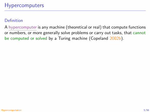
Hypercomputers
DefinitionA hypercomputer is any machine (theoretical or real) that compute functionsor numbers, or more generally solve problems or carry out tasks, that cannotbe computed or solved by a Turing machine (Copeland 2002b).
Super Turing Machines and Non Turing Machines
TMSuper-TM
𝐿 ⊆ Σ∗
non-TM
TM𝐿 ⊆ Σ∗
Hypercomputation 5/56
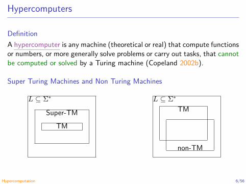
Hypercomputers
DefinitionA hypercomputer is any machine (theoretical or real) that compute functionsor numbers, or more generally solve problems or carry out tasks, that cannotbe computed or solved by a Turing machine (Copeland 2002b).
Super Turing Machines and Non Turing Machines
TMSuper-TM
𝐿 ⊆ Σ∗
non-TM
TM𝐿 ⊆ Σ∗
Hypercomputation 6/56
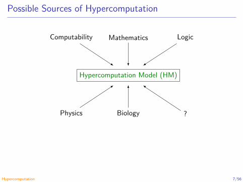
Possible Sources of Hypercomputation
MathematicsComputability Logic
Hypercomputation Model (HM)
BiologyPhysics ?
Hypercomputation 7/56

First Hypercomputation Model: Oracle Turing Machines
DefinitionA oracle Turing machine (OTM) is a Turing machine equipped with anoracle that is capable of answering questions about the membership of aspecific set of natural numbers (Turing 1939).
Hypercomputability featuresIf the oracle is a recursive set then OTM ≡ TM.If the oracle is a non-recursive set then OTM ≡ HM.
Hypercomputation 8/56

First Hypercomputation Model: Oracle Turing Machines
DefinitionA oracle Turing machine (OTM) is a Turing machine equipped with anoracle that is capable of answering questions about the membership of aspecific set of natural numbers (Turing 1939).
Hypercomputability featuresIf the oracle is a recursive set then OTM ≡ TM.If the oracle is a non-recursive set then OTM ≡ HM.
Hypercomputation 9/56
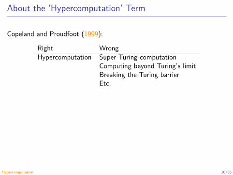
About the ‘Hypercomputation’ Term
Copeland and Proudfoot (1999):
Right WrongHypercomputation Super-Turing computation
Computing beyond Turing’s limitBreaking the Turing barrierEtc.
Hypercomputation 10/56
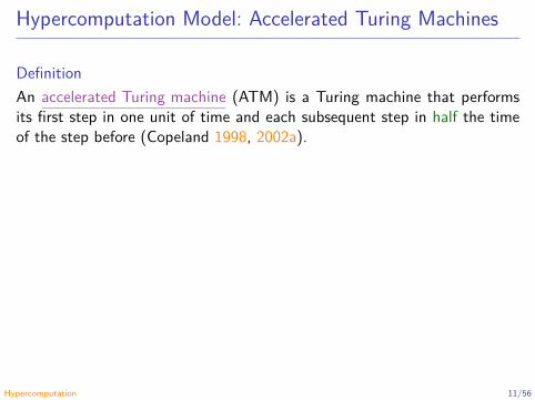
Hypercomputation Model: Accelerated Turing Machines
DefinitionAn accelerated Turing machine (ATM) is a Turing machine that performsits first step in one unit of time and each subsequent step in half the timeof the step before (Copeland 1998, 2002a).
Hypercomputability featuresSince
1 + 1/2 + 1/4 + 1/8 + … =∞
∑𝑖=0
12𝑖 = 2,
an ATM could complete an infinity of steps in two time units.
Hypercomputation 11/56
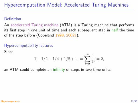
Hypercomputation Model: Accelerated Turing Machines
DefinitionAn accelerated Turing machine (ATM) is a Turing machine that performsits first step in one unit of time and each subsequent step in half the timeof the step before (Copeland 1998, 2002a).
Hypercomputability featuresSince
1 + 1/2 + 1/4 + 1/8 + … =∞
∑𝑖=0
12𝑖 = 2,
an ATM could complete an infinity of steps in two time units.
Hypercomputation 12/56
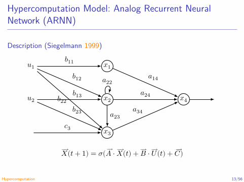
Hypercomputation Model: Analog Recurrent NeuralNetwork (ARNN)
Description (Siegelmann 1999)
𝑢1
𝑢2
𝑥1
𝑥2
𝑥3
𝑥4
𝑏11
𝑏12
𝑏13𝑏22𝑏23
𝑐3
𝑎14𝑎22
𝑎24
𝑎23𝑎34
𝑋(𝑡 + 1) = 𝜎( 𝐴 ⋅ 𝑋(𝑡) + 𝐵 ⋅ 𝑈(𝑡) + 𝐶)
Hypercomputation 13/56

Hypercomputation Model: Analog Recurrent NeuralNetwork (ARNN)
Hypercomputability features
𝑎𝑖𝑗 ∈ {ℕ, ℚ, ℝ} ⇒ ARNN ≡ {DFA, TM, HM}.
Hypercomputation 14/56
Standard Quantum Computation (SQC)
ModelsQuantum Turing machines (QTM) (Deutsch 1985) and quantum cir-cuits (Deutsch 1989).
Relation between the models
TMs Probabilistic TMs
Reversible TMs QTMs
≡
≡ ≡
≡
Hypercomputation 15/56
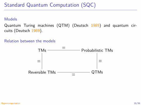
Standard Quantum Computation (SQC)
ModelsQuantum Turing machines (QTM) (Deutsch 1985) and quantum cir-cuits (Deutsch 1989).
Relation between the models
TMs Probabilistic TMs
Reversible TMs QTMs
≡
≡ ≡
≡
Hypercomputation 16/56
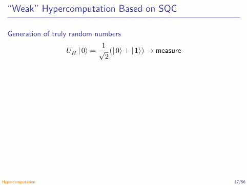
“Weak” Hypercomputation Based on SQC
Generation of truly random numbers
𝑈𝐻 | 0⟩ = 1√2
(| 0⟩ + | 1⟩) → measure
1. We observe the superposition state: “The act of observation causesthe superposition to collapse into either | 0⟩ or the | 1⟩ state withequal probability. Hence you can exploit quantum mechanicalsuperposition and indeterminism to simulate a perfectly fair cointoss.” (Williams and Clearwater 1997, p. 160)
2. The problem: It is not clear how to use this property to solve anon-computable Turing machine problem (Ord and Kieu 2009).
Hypercomputation 17/56
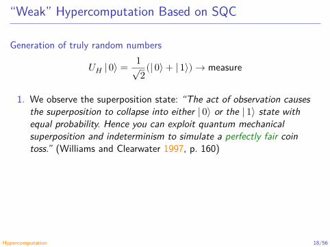
“Weak” Hypercomputation Based on SQC
Generation of truly random numbers
𝑈𝐻 | 0⟩ = 1√2
(| 0⟩ + | 1⟩) → measure
1. We observe the superposition state: “The act of observation causesthe superposition to collapse into either | 0⟩ or the | 1⟩ state withequal probability. Hence you can exploit quantum mechanicalsuperposition and indeterminism to simulate a perfectly fair cointoss.” (Williams and Clearwater 1997, p. 160)
2. The problem: It is not clear how to use this property to solve anon-computable Turing machine problem (Ord and Kieu 2009).
Hypercomputation 18/56

“Weak” Hypercomputation Based on SQC
Generation of truly random numbers
𝑈𝐻 | 0⟩ = 1√2
(| 0⟩ + | 1⟩) → measure
1. We observe the superposition state: “The act of observation causesthe superposition to collapse into either | 0⟩ or the | 1⟩ state withequal probability. Hence you can exploit quantum mechanicalsuperposition and indeterminism to simulate a perfectly fair cointoss.” (Williams and Clearwater 1997, p. 160)
2. The problem: It is not clear how to use this property to solve anon-computable Turing machine problem (Ord and Kieu 2009).
Hypercomputation 19/56

Others Quantum Computation Models
Common misunderstanding
quantum computation ≡ SQC≡ adiabatic quantum computation (AQC)
The real situationKieu’s hypercomputational quantum algorithm (KHQA) (Kieu 2003):
finite AQC ≡ SQCinfinite AQC ≡ KHQA
Hypercomputation 20/56

Others Quantum Computation Models
Common misunderstanding
quantum computation ≡ SQC≡ adiabatic quantum computation (AQC)
The real situationKieu’s hypercomputational quantum algorithm (KHQA) (Kieu 2003):
finite AQC ≡ SQCinfinite AQC ≡ KHQA
Hypercomputation 21/56

Hypercomputational Quantum Algorithm à la Kieu
Sicard, Ospina and Vélez (2006):
Classically non-computable 𝑃 problem
(Hilbert’s 10th problem)
Hypercomputationalquantum algorithm
Physical referent(Infinite square well)
Simulation
Dynamical algebra(Lie alg. 𝔰𝔲(1, 1))
Partialsolution
to 𝑃
Hypercomputation 22/56
Hypercomputation Model: Infinite Time Turing Machines
DefinitionAn infinite time Turing machine is a Turing machine working on a timeclocked by transfinite ordinals (Hamkins and Lewis 2000; Hamkins 2002,2007).
DescriptionFor convenience, the machines have three tapes:†
input:
scratch:
output:
start
1
0
0
1
0
0
0
0
0
1
0
0
1
0
0
0
0
0
· · ·
· · ·
· · ·
†Figure from Hamkins (2002, Fig. 1).Hypercomputation 23/56
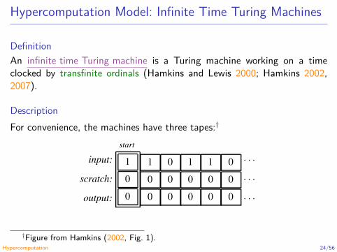
Hypercomputation Model: Infinite Time Turing Machines
DefinitionAn infinite time Turing machine is a Turing machine working on a timeclocked by transfinite ordinals (Hamkins and Lewis 2000; Hamkins 2002,2007).
DescriptionFor convenience, the machines have three tapes:†
input:
scratch:
output:
start
1
0
0
1
0
0
0
0
0
1
0
0
1
0
0
0
0
0
· · ·
· · ·
· · ·
†Figure from Hamkins (2002, Fig. 1).Hypercomputation 24/56
Hypercomputation Model: Infinite Time Turing Machines
Description (cont.)In stage 𝛼 + 1 the machine works as usual.
In limit ordinal stages the machine works as follows (Hamkins and Lewis2000, p. 569–570):“To set up such a limit ordinal configuration, the head is plucked fromwherever it might have been racing towards, and placed on top of the firstcell. And it is placed in a special distinguished limit state.”“Now we need to take a limit of the cell values on the tape. And we will dothis cell by cell according to the following rule: if the values appearing in acell have converged, that is, if they are either eventually 0 or eventually 1before the limit stage, then the cell retains the limiting value at the limitstage. Otherwise, in the case that the cell values have alternated from 0to 1 and back again unboundedly often, we make the limit cell value 1.”
Hypercomputation 25/56
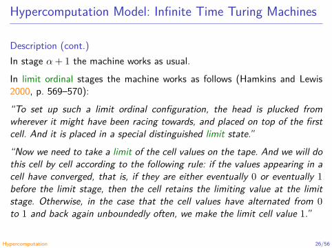
Hypercomputation Model: Infinite Time Turing Machines
Description (cont.)In stage 𝛼 + 1 the machine works as usual.In limit ordinal stages the machine works as follows (Hamkins and Lewis2000, p. 569–570):“To set up such a limit ordinal configuration, the head is plucked fromwherever it might have been racing towards, and placed on top of the firstcell. And it is placed in a special distinguished limit state.”“Now we need to take a limit of the cell values on the tape. And we will dothis cell by cell according to the following rule: if the values appearing in acell have converged, that is, if they are either eventually 0 or eventually 1before the limit stage, then the cell retains the limiting value at the limitstage. Otherwise, in the case that the cell values have alternated from 0to 1 and back again unboundedly often, we make the limit cell value 1.”
Hypercomputation 26/56
Hypercomputation Model: Infinite Time Turing Machines
Description (cont.)“This completely describes the configuration of the machine at any limitordinal stage 𝛽, and the machine can go on computing, 𝛽 + 1, 𝛽 + 2, andso on, eventually taking another limit at 𝛽 + 𝜔 co and so on through theordinals.”
Hypercomputability featuresThe halting problem is decidable in 𝜔 many steps by infinite time Turingmachines (Hamkins and Lewis 2000).
RemarkAlthough not related with computability but algorithmic complexity,𝑃 ≠ 𝑁𝑃 for infinite time Turing machines (Schindler 2003).
Hypercomputation 27/56
Hypercomputation Model: Infinite Time Turing Machines
Description (cont.)“This completely describes the configuration of the machine at any limitordinal stage 𝛽, and the machine can go on computing, 𝛽 + 1, 𝛽 + 2, andso on, eventually taking another limit at 𝛽 + 𝜔 co and so on through theordinals.”
Hypercomputability featuresThe halting problem is decidable in 𝜔 many steps by infinite time Turingmachines (Hamkins and Lewis 2000).
RemarkAlthough not related with computability but algorithmic complexity,𝑃 ≠ 𝑁𝑃 for infinite time Turing machines (Schindler 2003).
Hypercomputation 28/56
Hypercomputation Model: Infinite Time Turing Machines
Description (cont.)“This completely describes the configuration of the machine at any limitordinal stage 𝛽, and the machine can go on computing, 𝛽 + 1, 𝛽 + 2, andso on, eventually taking another limit at 𝛽 + 𝜔 co and so on through theordinals.”
Hypercomputability featuresThe halting problem is decidable in 𝜔 many steps by infinite time Turingmachines (Hamkins and Lewis 2000).
RemarkAlthough not related with computability but algorithmic complexity,𝑃 ≠ 𝑁𝑃 for infinite time Turing machines (Schindler 2003).
Hypercomputation 29/56
Hypercomputation Model: Infinite Time Turing Machines
Theorem (Hamkins and Lewis (2000, Theorem 1.1))Every halting infinite time computation is countable.
RemarkThe infinite time Turing machines have been generalised by theordinal computability models, which are models based on ordinal numbers.These models include infinite time Turing machines or Turing machinesworking on tapes of transfinite “length”. Seyfferth (2013) shows a briefoverview of these models.
Hypercomputation 30/56

Hypercomputation Model: Infinite Time Turing Machines
Theorem (Hamkins and Lewis (2000, Theorem 1.1))Every halting infinite time computation is countable.
RemarkThe infinite time Turing machines have been generalised by theordinal computability models, which are models based on ordinal numbers.These models include infinite time Turing machines or Turing machinesworking on tapes of transfinite “length”. Seyfferth (2013) shows a briefoverview of these models.
Hypercomputation 31/56

Church-Turing Thesis and Thesis M
The Church-Turing thesis“Any procedure than can be carried out by an idealised human clerk workingmechanically with paper and pencil can also be carried out by a Turingmachine.” (Copeland and Sylvan 1999)
Thesis M“What can be calculated by a machine is Turing machine comput-able.” (Gandy 1980)
Hypercomputation 32/56
Church-Turing Thesis and Thesis M
The Church-Turing thesis“Any procedure than can be carried out by an idealised human clerk workingmechanically with paper and pencil can also be carried out by a Turingmachine.” (Copeland and Sylvan 1999)
Thesis M“What can be calculated by a machine is Turing machine comput-able.” (Gandy 1980)
Hypercomputation 33/56
Physical Hypercomputation?
Open problemThe refutation of a general/physical version of Gandy’s Thesis M.
Based on quantum physics (infinite adiabatic quantum computation)?Based on relativistic physics (cosmological phenomena)? (Pitowsky1990; Hogarth 1992, 1994; Etesi and Németi 2002; Németi and Dávid2006)
Hypercomputation 34/56

Physical Hypercomputation?
Open problemThe refutation of a general/physical version of Gandy’s Thesis M.
Based on quantum physics (infinite adiabatic quantum computation)?
Based on relativistic physics (cosmological phenomena)? (Pitowsky1990; Hogarth 1992, 1994; Etesi and Németi 2002; Németi and Dávid2006)
Hypercomputation 35/56
Physical Hypercomputation?
Open problemThe refutation of a general/physical version of Gandy’s Thesis M.
Based on quantum physics (infinite adiabatic quantum computation)?Based on relativistic physics (cosmological phenomena)? (Pitowsky1990; Hogarth 1992, 1994; Etesi and Németi 2002; Németi and Dávid2006)
Hypercomputation 36/56
An Interesting Project: Formal Verification ofHypercomputation in Relativistic Physics
Stannett and Németi (2014) and Stannett (2015):
GoalsImplement first-order axiomatisations of theories of the relativityusing the proof assistant Isabelle;
Add a model of computation carried out by machines travelling alongspecific spacetime trajectories;
Hypercomputation 37/56
An Interesting Project: Formal Verification ofHypercomputation in Relativistic Physics
Stannett and Németi (2014) and Stannett (2015):
GoalsImplement first-order axiomatisations of theories of the relativityusing the proof assistant Isabelle;Add a model of computation carried out by machines travelling alongspecific spacetime trajectories;
Hypercomputation 38/56

An Interesting Project: Formal Verification ofHypercomputation in Relativistic Physics
Goals (cont.)Consider how the power of these computational systems changesaccording to the underlying topology of spacetime;
Select a recursively uncomputable problem 𝑃 (for example, theHalting Problem) and machine-verify the following claims:
in simpler relativistic settings, 𝑃 remains uncomputable;in some spacetimes, 𝑃 can be solved.
Hypercomputation 39/56
An Interesting Project: Formal Verification ofHypercomputation in Relativistic Physics
Goals (cont.)Consider how the power of these computational systems changesaccording to the underlying topology of spacetime;Select a recursively uncomputable problem 𝑃 (for example, theHalting Problem) and machine-verify the following claims:
in simpler relativistic settings, 𝑃 remains uncomputable;in some spacetimes, 𝑃 can be solved.
Hypercomputation 40/56
Is Hypercomputation a Myth?
Davis’ refutationsDavis, M. (2006). Why There is no Such Discipline asHypercomputation. Applied Mathematics and Computation 178.1,pp. 4–7. doi: 10.1016/j.amc.2005.09.066.
Davis, M. (2004). The Myth of Hypercomputation. In: Alan Turing:Life and Legaly of a Great Thinker. Ed. by Teuscher, C. Springer,pp. 195–211. doi: 10.1007/978-3-662-05642-4_8.
Refutation to DavisSundar, N. and Bringsjord, S. (2011). The Myth of ‘The Myth of Hyper-computation’. In: Combined Pre-Proceedings of P&C 2011 and HyperNet2011. Ed. by Stannett, M., pp. 185–196.
Hypercomputation 41/56

Is Hypercomputation a Myth?
Davis’ refutationsDavis, M. (2006). Why There is no Such Discipline asHypercomputation. Applied Mathematics and Computation 178.1,pp. 4–7. doi: 10.1016/j.amc.2005.09.066.Davis, M. (2004). The Myth of Hypercomputation. In: Alan Turing:Life and Legaly of a Great Thinker. Ed. by Teuscher, C. Springer,pp. 195–211. doi: 10.1007/978-3-662-05642-4_8.
Refutation to DavisSundar, N. and Bringsjord, S. (2011). The Myth of ‘The Myth of Hyper-computation’. In: Combined Pre-Proceedings of P&C 2011 and HyperNet2011. Ed. by Stannett, M., pp. 185–196.
Hypercomputation 42/56
Is Hypercomputation a Myth?
Davis’ refutationsDavis, M. (2006). Why There is no Such Discipline asHypercomputation. Applied Mathematics and Computation 178.1,pp. 4–7. doi: 10.1016/j.amc.2005.09.066.Davis, M. (2004). The Myth of Hypercomputation. In: Alan Turing:Life and Legaly of a Great Thinker. Ed. by Teuscher, C. Springer,pp. 195–211. doi: 10.1007/978-3-662-05642-4_8.
Refutation to DavisSundar, N. and Bringsjord, S. (2011). The Myth of ‘The Myth of Hyper-computation’. In: Combined Pre-Proceedings of P&C 2011 and HyperNet2011. Ed. by Stannett, M., pp. 185–196.
Hypercomputation 43/56
Academic Community
CommunitiesHypercomputation Research NetworkComputability in Europe (CiE)
Books and dedicated journal issuesSyropoulos, A. (2008). Hypercomputation. Computing Beyond theChurch-Turing Barrier. Springer.Applied Mathematics and Computation. Vol. 178(1), 2006.Burgin, M. (2005). Super-Recursive Algorithms. Springer.Theoretical Computer Science. Vol. 317(1-3), 2004.Mind and Machines. Vols. 12(4)/13(1), 2002/2003.
Hypercomputation 44/56
Academic Community
CommunitiesHypercomputation Research NetworkComputability in Europe (CiE)
Books and dedicated journal issuesSyropoulos, A. (2008). Hypercomputation. Computing Beyond theChurch-Turing Barrier. Springer.Applied Mathematics and Computation. Vol. 178(1), 2006.Burgin, M. (2005). Super-Recursive Algorithms. Springer.Theoretical Computer Science. Vol. 317(1-3), 2004.Mind and Machines. Vols. 12(4)/13(1), 2002/2003.
Hypercomputation 45/56

Final Remarks
“Once upon on time, back in the golden age of the recursive functiontheory, computability was an absolute.” (Sylvan and Copeland 2000,p. 189)
“Via the great pioneers of electronic computing…the 1930s analysis ofcomputation led to the modern computing era. Who knows where a21st-century overhaul of that classical analysis might lead.” (Copeland,Dresner, Proudfoot and Shagrir 2016, p. 38)“Is there any limit to discrete computation, and more generally, toscientific knowledge?” (Calude and Dinneen 1998, p. 1)““In breaking the Turing barrier, our knowledge of the world, and thereforeour control of it, would be altered forever,” Professor Cooper added.”†
†Computing a way through the Turing barrier. The Reporter. The University of LeedsNewsletter. No. 505. 21 February 2005.
Hypercomputation 46/56
Final Remarks
“Once upon on time, back in the golden age of the recursive functiontheory, computability was an absolute.” (Sylvan and Copeland 2000,p. 189)“Via the great pioneers of electronic computing…the 1930s analysis ofcomputation led to the modern computing era. Who knows where a21st-century overhaul of that classical analysis might lead.” (Copeland,Dresner, Proudfoot and Shagrir 2016, p. 38)
“Is there any limit to discrete computation, and more generally, toscientific knowledge?” (Calude and Dinneen 1998, p. 1)““In breaking the Turing barrier, our knowledge of the world, and thereforeour control of it, would be altered forever,” Professor Cooper added.”†
†Computing a way through the Turing barrier. The Reporter. The University of LeedsNewsletter. No. 505. 21 February 2005.
Hypercomputation 47/56
Final Remarks
“Once upon on time, back in the golden age of the recursive functiontheory, computability was an absolute.” (Sylvan and Copeland 2000,p. 189)“Via the great pioneers of electronic computing…the 1930s analysis ofcomputation led to the modern computing era. Who knows where a21st-century overhaul of that classical analysis might lead.” (Copeland,Dresner, Proudfoot and Shagrir 2016, p. 38)“Is there any limit to discrete computation, and more generally, toscientific knowledge?” (Calude and Dinneen 1998, p. 1)
““In breaking the Turing barrier, our knowledge of the world, and thereforeour control of it, would be altered forever,” Professor Cooper added.”†
†Computing a way through the Turing barrier. The Reporter. The University of LeedsNewsletter. No. 505. 21 February 2005.
Hypercomputation 48/56

Final Remarks
“Once upon on time, back in the golden age of the recursive functiontheory, computability was an absolute.” (Sylvan and Copeland 2000,p. 189)“Via the great pioneers of electronic computing…the 1930s analysis ofcomputation led to the modern computing era. Who knows where a21st-century overhaul of that classical analysis might lead.” (Copeland,Dresner, Proudfoot and Shagrir 2016, p. 38)“Is there any limit to discrete computation, and more generally, toscientific knowledge?” (Calude and Dinneen 1998, p. 1)““In breaking the Turing barrier, our knowledge of the world, and thereforeour control of it, would be altered forever,” Professor Cooper added.”†
†Computing a way through the Turing barrier. The Reporter. The University of LeedsNewsletter. No. 505. 21 February 2005.
Hypercomputation 49/56
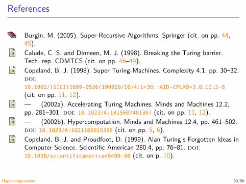
References
Burgin, M. (2005). Super-Recursive Algorithms. Springer (cit. on pp. 44,45).Calude, C. S. and Dinneen, M. J. (1998). Breaking the Turing barrier.Tech. rep. CDMTCS (cit. on pp. 46–49).Copeland, B. J. (1998). Super Turing-Machines. Complexity 4.1, pp. 30–32.doi:10.1002/(SICI)1099-0526(199809/10)4:1<30::AID-CPLX9>3.0.CO;2-8(cit. on pp. 11, 12).— (2002a). Accelerating Turing Machines. Minds and Machines 12.2,pp. 281–301. doi: 10.1023/A:1015607401307 (cit. on pp. 11, 12).— (2002b). Hypercomputation. Minds and Machines 12.4, pp. 461–502.doi: 10.1023/A:1021105915386 (cit. on pp. 5, 6).Copeland, B. J. and Proudfoot, D. (1999). Alan Turing’s Forgotten Ideas inComputer Science. Scientific American 280.4, pp. 76–81. doi:10.1038/scientificamerican0499-98 (cit. on p. 10).
Hypercomputation 50/56

References
Copeland, B. J. and Sylvan, R. (1999). Beyond the Universal TuringMachine. Australasian Journal of Philosophy 77.1, pp. 44–66. doi:10.1080/00048409912348801 (cit. on pp. 32, 33).Copeland, J., Dresner, E., Proudfoot, D. and Shagrir, O. (2016). Time toReinspect the Foundations? Communications of the ACM 59.11, pp. 34–38.doi: 10.1145/2908733 (cit. on pp. 46–49).Davis, M. (1958). Computability and Unsolvability. McGraw-Hill (cit. onp. 3).— (2004). The Myth of Hypercomputation. In: Alan Turing: Life andLegaly of a Great Thinker. Ed. by Teuscher, C. Springer, pp. 195–211. doi:10.1007/978-3-662-05642-4_8 (cit. on pp. 41–43).— (2006). Why There is no Such Discipline as Hypercomputation.Applied Mathematics and Computation 178.1, pp. 4–7. doi:10.1016/j.amc.2005.09.066 (cit. on pp. 41–43).Deutsch, D. (1985). Quantum Theory, the Church-Turing Principle and theUniversal Quantum Computer. Proc. R. Soc. Lond. A 400, pp. 97–117.doi: 10.1098/rspa.1985.0070 (cit. on pp. 15, 16).
Hypercomputation 51/56

References
Deutsch, D. (1989). Quantum Computational Networks. Proc. R. Soc.Lond. A 425, pp. 73–90. doi: 10.1098/rspa.1989.0099 (cit. on pp. 15, 16).Etesi, G. and Németi, I. (2002). Non-Turing Computations ViaMalament-Hogart Space-Times. Int. J. Theor. Phys. 41.2, pp. 341–370.doi: 10.1023/A:1014019225365 (cit. on pp. 34–36).Gandy, R. (1980). Church’s Thesis and Principles for Mechanisms. In: TheKleene Symposium. Ed. by Barwise, J., Keisler, H. J. and Kunen, K.Vol. 101. Studies in Logic and the Foundations of Mathematics.North-Holland Publishing Company, pp. 123–148. doi:10.1016/S0049-237X(08)71257-6 (cit. on pp. 32, 33).Gödel, K. (1990). Remarks Before the Princeton Bicentennial Conferenceon Problems in Mathematics (1946). In: Kurt Gödel. Collected works.Ed. by Feferman, S. et al. Vol. I. Publications 1938–1974. Oxford UniversityPress, pp. 150–153 (cit. on p. 2).Hamkins, J. D. (2002). Infinite Time Turing machines. Minds and Machines12.4, pp. 521–539. doi: 10.1023/A:1021180801870 (cit. on pp. 23, 24).
Hypercomputation 52/56

References
Hamkins, J. D. (2007). A Survey of Infinite time Turing machines. In:Machines, Computations, and Universality (MCU 2007). Ed. byDurand-Lose, J. and Margenstern, M. Vol. 4664. Lecture Notes inComputer Science, pp. 62–71. doi: 10.1007/978-3-540-74593-8_5 (cit. onpp. 23, 24).Hamkins, J. D. and Lewis, A. (2000). Infinite Time Turing machines. TheJournal of Symbolic Logic 65.2, pp. 567–604. doi: 10.2307/2586556(cit. on pp. 23–31).Hogarth, M. (1992). Does General Relativity Allow an Observer to View anEternity in a Finite Time? Foundations on Physics Letters 5.2, pp. 173–181.doi: 10.1007/BF00682813 (cit. on pp. 34–36).— (1994). Non-Turing Computers and Non-Turing Computability. PSA1994, pp. 126–138 (cit. on pp. 34–36).Kieu, T. D. (2003). Computing the Non-Computable. ContemporaryPhysics 44.1, pp. 51–71. doi: 10.1080/00107510302712 (cit. on pp. 20, 21).
Hypercomputation 53/56

References
Németi, I. and Dávid, G. (2006). Relativistic Computers and the TuringBarrier. Applied Mathematics and Computation 178.1, pp. 118–142. doi:10.1016/j.amc.2005.09.075 (cit. on pp. 34–36).Ord, T. and Kieu, T. D. (2009). Using Biased Coins as Oracles.International Journal of Unconventional Computing 5, pp. 253–265 (cit. onpp. 17–19).Pitowsky, I. (1990). The Physical Church Thesis and PhysicalComputational Complexity. Iyyun 39, pp. 81–99. url:http://www.jstor.org/stable/23350656 (cit. on pp. 34–36).Schindler, R. (2003). 𝑃 ≠ 𝑁𝑃 for Infinite Time Turing Machines.Monatshefte für Mathematik 139.4, pp. 335–340. doi:10.1007/s00605-002-0545-5 (cit. on pp. 27–29).Seyfferth, B. (2013). Three Models of Ordinal Computability. PhD thesis.University of Bonn. url:http://hss.ulb.uni-bonn.de/2013/3196/3196.pdf (visited on14/05/2018) (cit. on pp. 30, 31).
Hypercomputation 54/56
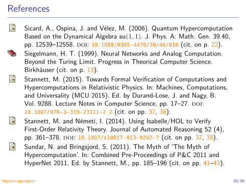
References
Sicard, A., Ospina, J. and Vélez, M. (2006). Quantum HypercomputationBased on the Dynamical Algebra 𝔰𝔲(1, 1). J. Phys. A: Math. Gen. 39.40,pp. 12539–12558. doi: 10.1088/0305-4470/39/40/018 (cit. on p. 22).Siegelmann, H. T. (1999). Neural Networks and Analog Computation.Beyond the Turing Limit. Progress in Theorical Computer Science.Birkhäuser (cit. on p. 13).Stannett, M. (2015). Towards Formal Verification of Computations andHypercomputations in Relativistic Physics. In: Machines, Computations,and Universality (MCU 2015). Ed. by Durand-Lose, J. and Nagy, B.Vol. 9288. Lecture Notes in Computer Science, pp. 17–27. doi:10.1007/978-3-319-23111-2_2 (cit. on pp. 37, 38).Stannett, M. and Németi, I. (2014). Using Isabelle/HOL to VerifyFirst-Order Relativity Theory. Journal of Automated Reasoning 52 (4),pp. 361–378. doi: 10.1007/s10817-013-9292-7 (cit. on pp. 37, 38).Sundar, N. and Bringsjord, S. (2011). The Myth of ‘The Myth ofHypercomputation’. In: Combined Pre-Proceedings of P&C 2011 andHyperNet 2011. Ed. by Stannett, M., pp. 185–196 (cit. on pp. 41–43).
Hypercomputation 55/56

References
Sylvan, R. and Copeland, J. (2000). Computability is Logic-Relative. In:Sociative Logics and Their Applications: Essays by the late Richard Sylvan.Ed. by Priest, G. and Hyde, D. Ashgate Publishing Company, pp. 189–199(cit. on pp. 4, 46–49).Syropoulos, A. (2008). Hypercomputation. Computing Beyond theChurch-Turing Barrier. Springer (cit. on pp. 44, 45).Turing, A. M. (1939). Systems of Logic Based on Ordinales. Proc. LondonMath. Soc. 45.2239, pp. 161–228. doi: 10.1112/plms/s2-45.1.161 (cit. onpp. 8, 9).Williams, C. P. and Clearwater, S. H. (1997). Explorations in QuantumComputing. Springer-Telos (cit. on pp. 17–19).
Hypercomputation 56/56