Embed Size (px)
Citation preview

AutoGF: An Automated System to Calculate Coefficients of
Generating Functions
by
Huantian Cao
(Under the direction of Robert W. Robinson)
Abstract
AutoGF, an automated system to calculate coefficients of generating functions,is developed in this thesis. The algorithms for power series manipulations such asaddition, substraction, multiplication, division, powers, exponentiation, logorithm,reversion and composition are implemented in AutoGF. Maclaurin series provide thebasis for calculating the coefficients of basic generating functions. User defined gener-ating functions are also provided for. By writing a text file listing the algebraic stepsdefining a target generating function, the user of AutoGF can obtain the coefficientsof very complicated generating functions.
Exponential generating functions are widely used to count labeled graphs anddigraphs. By applying a Hadamard product to the coefficients of exponential gen-erating functions, the exact numbers of labeled graphs or digraphs with differentnumbers of vertices can be obtained under various restrictions using AutoGF. Thisis demonstrated for connected graphs, blocks, connected eulerian graphs, acyclicdigraphs, strong digraphs, and forests. The time performances of these graphicalenumerations are investigated and their time complexities are estimated.
Generating functions can also be applied to count integer partitions. The numbersof all partitions and of partitions into distinct parts are calculated by using AutoGF.The time performances of these partition enumerations are investigated and theirtime complexities are estimated.
Index words: Generating Function, Exponential Generating Function, PowerSeries, Graph Enumeration, Integer Partitions, Python

AutoGF: An Automated System to Calculate Coefficients of
Generating Functions
by
Huantian Cao
B.S., China Textile University, China, 1994
M.S., China Textile University, China, 1997
Ph.D., The University of Georgia, 2000
A Thesis Submitted to the Graduate Faculty
of The University of Georgia in Partial Fulfillment
of the
Requirements for the Degree
Master of Science
Athens, Georgia
2002
c© 2002
Huantian Cao
All Rights Reserved
AutoGF: An Automated System to Calculate Coefficients of
Generating Functions
by
Huantian Cao
Approved:
Major Professor: Robert W. Robinson
Committee: E. Rodney Canfield
David Gries
Electronic Version Approved:
Gordhan L. Patel
Dean of the Graduate School
The University of Georgia
May 2002
Acknowledgments
The author would like to express his deep appreciation to his major professor, Dr.
Robert W. Robinson, for his remarkable encouragement, support, guidance, assis-
tance, and kindness. Without Dr. Robinson’s advice and effort, completion of this
thesis would have been impossible.
The author is thankful to Dr. E. Rodney Canfield and Dr. David Gries for serving
on his thesis committee. The author expresses his gratitude to Dr. Michael A. Cov-
inton for providing LATEX style sheet uga.sty to make it easier to type this thesis.
The author appreciates the faculty, staff, and graduate students of the Department
of Computer Science for their cooperation and help.
The author is thankful for the financial assistance provided by the Deaprtment
of Computer Science and the Department of Textiles, Merchandising and Interiors
of the University of Georgia.
iv

Table of Contents
Page
Acknowledgments . . . . . . . . . . . . . . . . . . . . . . . . . . . . . iv
List of Tables . . . . . . . . . . . . . . . . . . . . . . . . . . . . . . . vii
Chapter
1 Introduction . . . . . . . . . . . . . . . . . . . . . . . . . . . . 1
1.1 Generating Functions . . . . . . . . . . . . . . . . . . 1
1.2 Purpose of This Study . . . . . . . . . . . . . . . . . . 4
2 Algorithms For Manipulating Generating Functions . . . 6
2.1 Rational Arithmetic . . . . . . . . . . . . . . . . . . . 6
2.2 Expansions of Basic Functions . . . . . . . . . . . . . 7
2.3 Manipulation of Generating Functions . . . . . . . . 8
3 The Implementation of AutoGF . . . . . . . . . . . . . . . . . . 16
3.1 Python . . . . . . . . . . . . . . . . . . . . . . . . . . . . 16
3.2 The Architecture of AutoGF . . . . . . . . . . . . . . . 18
3.3 How to Use The System . . . . . . . . . . . . . . . . . 20
4 Applications of AutoGF to Labeled Graph Enumeration . . 23
4.1 Connected Labeled Graphs . . . . . . . . . . . . . . . 23
4.2 Labeled Blocks . . . . . . . . . . . . . . . . . . . . . . 25
4.3 Connected Labeled Eulerian Graphs . . . . . . . . . 28
4.4 Labeled Acyclic Digraphs . . . . . . . . . . . . . . . . 31
v
vi
4.5 Labeled Strong Digraphs . . . . . . . . . . . . . . . . 35
4.6 Labeled Trees and Forests . . . . . . . . . . . . . . . 38
5 Applications of AutoGF to Counting Integer Partitions . . 44
6 Conclusion . . . . . . . . . . . . . . . . . . . . . . . . . . . . . 51
Bibliography . . . . . . . . . . . . . . . . . . . . . . . . . . . . . . . . 54

List of Tables
4.1 Number of Connected Labeled Graphs . . . . . . . . . . . . . . . . . 26
4.2 Time Performance of Connected Labeled Graphs . . . . . . . . . . . . 27
4.3 Number of Labeled Blocks . . . . . . . . . . . . . . . . . . . . . . . . 29
4.4 Time Performance of Labeled Blocks . . . . . . . . . . . . . . . . . . 30
4.5 Number of Connected Labeled Eulerian Graphs . . . . . . . . . . . . 32
4.6 Time Performance of Connected Labeled Eulerian Graphs . . . . . . 33
4.7 Number of Labeled Acyclic Digraphs . . . . . . . . . . . . . . . . . . 34
4.8 Time Performance of Labeled Acyclic Digraphs . . . . . . . . . . . . 35
4.9 Number of Labeled Strong Digraphs . . . . . . . . . . . . . . . . . . 37
4.10 Time Performance of Labeled Strong Digraphs . . . . . . . . . . . . . 38
4.11 Number of Labeled Trees . . . . . . . . . . . . . . . . . . . . . . . . . 40
4.12 Time Performance of Labeled Trees . . . . . . . . . . . . . . . . . . . 41
4.13 Number of Labeled Forests . . . . . . . . . . . . . . . . . . . . . . . . 42
4.14 Time Performance of Labeled Forests . . . . . . . . . . . . . . . . . . 43
5.1 Number of Unrestricted Partitions . . . . . . . . . . . . . . . . . . . . 46
5.2 Time Performance of Unrestricted Partitions . . . . . . . . . . . . . . 47
5.3 Number of Partitions with Distinct Parts . . . . . . . . . . . . . . . . 49
5.4 Time Performance of Partitions into Distinct Parts . . . . . . . . . . 50
6.1 Time Complexity of Graph Enumerations . . . . . . . . . . . . . . . 52
6.2 Time Complexity of Integer Partition Enumerations . . . . . . . . . . 52
vii
Chapter 1
Introduction
1.1 Generating Functions
A generating function is a power series whose coefficients are a sequence of numbers,
a0, a1, a2, · · · (Wilf 1990, p. 1). That is, g(x) is a generating function for ar if g(x)
has the polynomial expansion
g(x) = a0 + a1x + a2x2 + · · ·+ arx
r + · · ·+ anxn.
If the function has an infinite number of terms, it is called a power series (Tucker
1995, p. 243). In the application of generating functions, it does not matter whether
the power series converges, all power series discussed in this thesis are formal power
series meaning that we are not concerned with questions of convergence (Brent and
Kung 1978).
For a problem whose answer is a sequence of numbers, a0, a1, a2, · · · , an explicit
formula such as
an = n2 + 2n + 1,
or a recurrence relation such as
Fn+1 = Fn + Fn−1, (n ≥ 1; F0 = 0, F1 = 1)
may be available to calculate the terms. However, there are situations where a simple
formula or a recurrence relation does not exist or is hard to obtain. In these situ-
ations, relations involving generating functions may be another useful way to deal
with the sequence of numbers problem.
1
2
For example, we have the Fibonacci numbers F0, F1, F2, · · · , where
Fn+1 = Fn + Fn−1, (n ≥ 1; F0 = 0, F1 = 1).
The sequence begins with 0, 1, 1, 2, 3, 5, 8, 13, 21, 34, 55, 89, · · ·. But in addition to the
recurrence relation, we can also use the generating function
f(x) =x
1− x− x2
to represent the sequence of Fibonacci numbers. That is, the nth Fibonacci number,
Fn, is the coefficient of xn in the expansion of the function x/(1−x−x2) as a power
series about x = 0.
The generating functions discussed above are called ordinary generating func-
tions . They are used to model selection with repetition problems. There is another
category of generating functions called exponential generating functions , which are
usually used to model and solve problems involving arrangements and distributions
of distinct objects. An exponential generating function g(x) for ar is a function with
the power series expansion (Tucker 1995, p. 267):
g(x) = a0 + a1x + a2x2
2!+ a3
x3
3!+ · · ·+ ar
xr
r!+ · · ·
Exponential generating functions are defined in the same way as ordinary generating
functions except that each power xr is divided by r!. For a given expanded expo-
nential generating function, ar can be obtained by the operation of the Hadamard
product (@), which is defined as
< fi > @ < gi >=< figi >
Like exact formulas and recurrence relations, generating functions allow the user
to do almost anything he wants to do with a sequence. In many cases, the generating
functions are elegant, simple and easy to handle when exact formulas and recurrence
relations are very complicated or very difficult to find.

3
In his book Generatingfunctionology , Herbert S. Wilf described things that gen-
erating functions can do (Wilf 1990, p. 2).
(a) Find an exact formula for the sequence numbers. Generating functions cannot
guarantee to find the exact formula, but they provide a powerful way to find exact
formulas in some cases.
(b) Find a recurrence relation. Usually generating functions are obtained from
recurrence relations. However, from a generating function, the user may derive a new
recurrence relation and gain new insight into the nature of the sequence.
(c) Find the average and other statistical properties of the sequence. Generating
functions can provide quick ways to calculate probabilistic aspects of the problem
represented by a sequence of numbers.
(d) Find an asymptotic formula for the sequence. For some cases, it is impossible
to derive an the exact formula for a sequence, but an approximate formula may be
obtained by using generating functions.
(e) Prove unimodality, convexity, etc. A sequence is called unimodal if it increases
steadily at first and then decreases steadily. By analyzing a generating function, one
may be able to analyze the rises and falls of the sequence of coefficients.
(f) Prove identities. The identities referred to here are those in which a certain
formula is asserted to be equal to another formula for stated values of the free
variables. To prove this, we can define a generating function whose coefficients are
the sequence shown on the left side of the identity and a generating function whose
coefficients are the sequence shown on the right side of the identity and show that
they are the same function.
(g) Other. Generating functions may offer a way for the user who wants to
know something else about the sequence. For example, if a generating function has
a striking resemblance to some other known generating functions. This may lead the
user to discover that the problem is closely related to another one.

4
1.2 Purpose of This Study
In the application of generating functions, usually a generating function is obtained
as a result for a sequence of numbers. However, for a generating function, like
F (x) =x
1− x− x2,
it is highly desired to know the sequence numbers it represents. That is, we want to
know a0, a1, a2, · · · , ar, · · · , such that
x
1− x− x2= a0 + a1x + a2x
2 + · · ·+ arxr + · · · .
Because computer memory is finite, the user must specify a bound N so that coef-
ficients are calculated and stored only for powers less than N .
The purpose of the study is to develop an automatic system, called AutoGF,
to calculate coefficients of generating functions. The user of AutoGF must analyze
the generating function and express it in terms of simple or standard generating
functions and operations on them. AutoGF can then carry out the manipulation of
generating functions and calculate the coefficients. For example, for the generating
function
F (x) =x
1− x− x2,
we can divide it into two simple generating functions,
f(x) = x,
whose coefficients are 0, 1, 0, 0, 0, · · · and
g(x) = 1− x− x2,
whose coefficients are 1,−1,−1, 0, 0, · · ·, and use the division operation
F (x) =f(x)
g(x)

5
to express F (x).
Exponential generating functions are widely used in graph enumeration. In this
thesis, AutoGF is used with exponential generating functions to obtain the numbers of
connected labeled graphs, labeled blocks, connected labeled eulerian graphs, labeled
acyclic digraphs, labeled strong digraphs, labeled trees, and labeled forests. AutoGF
is also used with ordinary generating functions to count general integer partitions
and partitions into distinct parts. The amounts of time used to obtain these numbers
are measured and the time complexities are estimated. These experiments serve as
test cases for AutoGF since all of these numbers had been calculated previously.

Chapter 2
Algorithms For Manipulating Generating Functions
2.1 Rational Arithmetic
To calculate quantities defined by generating functions, it is desirable to calculate
the coefficients exactly rather than as floating point values. To accomplish this,
coefficients are represented as rational numbers with no preset limits on the size
of the numerator or denominator. Rational numbers can be represented as pairs of
integers (u/u′), where u′ 6= 0. The operations on two rational numbers (u/u′) (for
u′ 6= 0) and (v/v′) (for v′ 6= 0) are as follows:
u
u′± v
v′=
uv′ ± u′vu′v′
,
u
u′× v
v′=
uv
u′v′,
u
u′÷ v
v′=
uv′
u′v(v′ 6= 0).
If the numerator a and denominator a′ of the result are not relative prime, it is usually
best for efficiency to compute the greatest common divisor d = gcd(a, a′) and reduce
the fraction to w/w′ where w = a/d and w′ = a′/d. The modern Euclidean algorithm
(Knuth 1998, Algorithm A, p. 337), described below, is used to determine greatest
common divisor in this thesis.
Given nonnegative integers u and v, this algorithm finds their greatest common
divisor. The greatest common divisor of arbitrary integers u and v may be obtained
by applying the algorithm to |u| and |v| because
gcd(u, v) = gcd(v, u)
6

7
and
gcd(u, v) = gcd(−u, v)
1. [v = 0?] If v = 0, the algorithm terminates with u as the answer.
2. [Take u mod v.] Set r ← u mod v, u ← v, v ← r, and return to step 1. Application
of step 2 decreases the value of v but leaves gcd(u, v) unchanged.
2.2 Expansions of Basic Functions
For efficiency, it is helpful for a generatingfunctionologist to have available a reference
list of known power series and other series that occur frequently in applications. In
our system for automatically calculating coefficients of complicated generating func-
tions, these basic power series serve as bricks for the building since many complicated
generating functions are obtained from the manipulations of these basic power series.
The Maclaurin series generated by a function f , which is the Taylor series for
f at x = 0, can often be used to expand functions and produce useful power series
(Finney et al. 2000, p. 671). The Maclaurin series generated by the function f is
∞∑
k=0
f (k)(0)
k!xk = f(0) + f ′(0)x +
f ′′(0)
2!x2 + · · ·+ f (n)(0)
n!xn + · · · .
For example, we can use a Maclaurin series to expand ex as follows. Since
f(x) = ex, f ′(x) = ex, · · · , f (n)(x) = ex, · · · ,
we have
f(0) = e0 = 1, f ′(0) = e0 = 1, · · · , f (n)(0) = e0 = 1, · · · .
The Maclaurin series generated by f(x) = ex is
f(0) + f ′(0)x +f ′′(0)
2!x2 + · · ·+ f (n)(0)
n!xn + · · · = 1 + x +
1
2!x2 + · · ·+ 1
n!xn + · · · .
That is,
ex = 1 + x +1
2!x2 + · · ·+ 1
n!xn + · · · .

8
Here is a list of basic power series used in this study.
(1 + x)n = 1 + nx +n(n− 1)
2x2 + · · ·+ xn =
n∑
k=0
(n
k
)xk
ex = 1 + x +1
2!x2 + · · · =
∞∑
k=0
1
k!xk
ln(1 + x) = x− 1
2x2 +
1
3x3 + · · · =
∞∑
k=0
(−1)k+1
kxk
ln1
1− x= x +
1
2x2 +
1
3x3 + · · · =
∞∑
k=0
1
kxk
1
1− x= 1 + x + x2 + · · · =
∞∑
k=0
xk
1
1 + x= 1− x + x2 − · · · =
∞∑
k=0
(−1)kxk
sin x = x− x3
3!+
x5
5!+ · · · =
∞∑
k=0
(−1)k x2k+1
(2k + 1)!
cos x = 1− x2
2!+
x4
4!− · · · =
∞∑
k=0
(−1)k x2k
(2k)!
arctan x = x− x3
3+
x5
5− · · · =
∞∑
k=0
(−1)k x2k+1
2k + 1
sinh x =ex − e−x
2= x +
x3
3+
x5
5+ · · · =
∞∑
k=0
x2k+1
(2k + 1)!
cosh x =ex + e−x
2= 1 +
x2
2+
x4
4+ · · · =
∞∑
k=0
x2k
(2k)!
2.3 Manipulation of Generating Functions
For two generating functions
U(x) = U0 + U1x + U2x2 + · · ·
and
V (x) = V0 + V1x + V2x2 + · · · ,

9
their sum, difference, product, quotient, and composition can be used to express new
generating functions. For one generating function, its powers, exponential, logarithm
and reversion can also be used to form new generating functions. Because only a finite
number of terms can be represented and stored in a computer, we work only with the
first N coefficients of any generating function, where N is a user-specified bound. In
the following sections, we use [xn]W (x) to denote the nth coefficient of generating
function W (x).
2.3.1 Sum and Difference of Generating Functions
For the sum and difference of two generating functions, W (x) = U(x) ± V (x), the
coefficients of W (x) can be computed termwize (Knuth 1998, p. 525):
[xn](U(x)± V (x)) = Un ± Vn.
2.3.2 Product of Generating Functions
The convolution rule is used to calculate the coefficients of W (x) = U(x)V (x) (Knuth
1998, p. 525):
Wn = [xn]W (x) =n∑
k=0
UkVn−k = U0Vn + U1Vn−1 + · · ·+ UnV0.
The termwize or Hadamard product is essential to easily create exponential gen-
erating functions and obtain exact numbers from them. We use @ to represent
Hadamard product: W (x) = U(x)@V (x), where
Wn = [xn]W (x) = UnVn.
10
2.3.3 Quotient of Generating Functions
The rule to obtain the quotient W (x) = U(x)/V (x), when V0 6= 0, is to interchange
U and W in the previous formula for multiplication (Knuth 1998, p. 525):
Wn =Un −∑n−1
k=0 WkVn−k
V0
=Un −W0Vn −W1Vn−1 − · · · −Wn−1V1
V0
.
In some cases, the quotient of generating function W (x) = U(x)/V (x) can also be
calculated when V0 = 0. Let
U(x) = Ukxk + Uk+1x
k+1 + · · ·
and
V (x) = Vmxm + Vm+1xm+1 + · · ·
where Uk is the first non-zero coefficient of U(x) and Vm is the first non-zero coeffi-
cient of V (x). Coefficients of generating function W (x) = U(x)/V (x) can be calcu-
lated when k ≥ m since
U(x)
V (x)=
U(x)/xm
V (x)/xm
and the first m zero coefficients of denominator and numerator can be removed.
2.3.4 Powers of Generating Functions
For W (x) = V (x)α, where α is an arbitrary power, and Vm is the first nonzero
coefficient of V (x), we have
V (x) = Vmxm(1 + (Vm+1/Vm)x + (Vm+1/Vm)x2 + · · ·)
and
V (x)α = V αmxαm(1 + (Vm+1/Vm)x + (Vm+1/Vm)x2 + · · ·)α.
This will be a power series if and only if αm is a nonnegative integer. The operation
of computing W (x) = V (x)α, where α is an arbitrary power, can thus be reduced to

11
the case that V0 = 1 and
W (x) = (1 + V1x + V2x2 + V3x
3 + · · ·)α
Clearly W0 = 1α = 1.
In 1748, Leonhard Euler published a simple and efficient way to compute powers
of power series (Knuth 1998, p. 526). If W (x) = V (x)α, then by differentiation, we
get
W1 + 2W2x + 3W3x2 + · · · = W ′(x) = αV (x)α−1V ′(x)
and therefore
W ′(x)V (x) = αW (x)V ′(x).
Equating the coefficients of xn−1, we find
n∑
k=0
kWkVn−k = αn∑
k=0
(n− k)WkVn−k.
This gives us a useful computational rule valid for all n ≥ 1 and thus a simple online
algorithm to successively compute W1,W2, · · ·:
Wn =n∑
k=1
((α + 1
n)k − 1)VkWn−k
=(α + 1− n)V1Wn−1 + · · ·+ (kα− (n− k))VkWn−k + · · ·+ nαVnW0
n.
For us, α must be rational. In case α is not an integer, V (x)α is not unique so W (x)
represents just one of the possible values for V (x)α. In most applications, the desired
value for V (x)α will be W (x) or −W (x).
Online algorithms are used in this power operation and the operations discussed
below. Here online algorithm means that the calculation of the nth coefficient is based
on the n − 1 coefficients obtained previously instead of from user input numbers.
Online algorithms save space (and hence, to some extent, time) compared to offline
algorithms.

12
2.3.5 Exponential of Generating Functions
The calculation of coefficients of the exponential of a generating function, W (x) =
eU(x), where U0 = 0, is similar to the calculation of the powers of generating functions.
Differentiation of W (x) gives rise to a useful recurrence, as follows:
W (0) = eU(0) = e0 = 1;
W ′(x) = eU(x)U ′(x) = W (x)U ′(x).
Equating the coefficients of xn−1, we have for all n ≥ 1
nWn =n∑
k=1
Wn−kkUk.
This gives us a useful computational rule valid for all n ≥ 1 and thus a simple online
algorithm to successively compute W1,W2, · · ·:
Wn =1
n
n∑
k=1
Wn−kkUk.
2.3.6 Logarithm of Generating Functions
The reversion of the exponential of generating functions is the logarithm of gener-
ating functions. That is, if
W (x) = eU(x)
then
U(x) = ln(W (x)).
Here W0 = 1 and U0 = 0. From the exponential relation we have
Wn =1
n
n∑
k=1
Wn−kkUk,
hence
Wn =1
n
n−1∑
k=1
Wn−kkUk +1
nnUn,
13
and so (for n ≥ 1)
Un = Wn − 1
n
n−1∑
k=1
kUkWn−k.
The initial values for this formula are W0 = 1 and U0 = 0. We can also use this
formula to calculate the coefficients of U(x) = ln(1+V (x)) with V0 = 0 and U0 = 0.
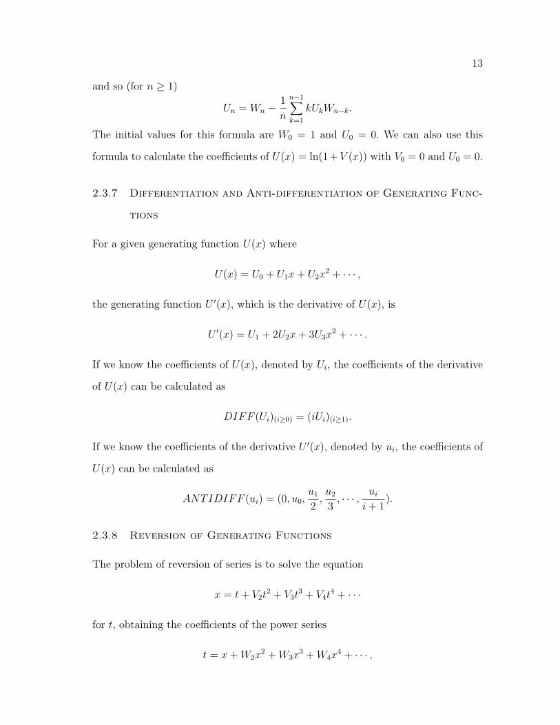
2.3.7 Differentiation and Anti-differentiation of Generating Func-
tions
For a given generating function U(x) where
U(x) = U0 + U1x + U2x2 + · · · ,
the generating function U ′(x), which is the derivative of U(x), is
U ′(x) = U1 + 2U2x + 3U3x2 + · · · .
If we know the coefficients of U(x), denoted by Ui, the coefficients of the derivative
of U(x) can be calculated as
DIFF (Ui)(i≥0) = (iUi)(i≥1).
If we know the coefficients of the derivative U ′(x), denoted by ui, the coefficients of
U(x) can be calculated as
ANTIDIFF (ui) = (0, u0,u1
2,u2
3, · · · , ui
i + 1).
2.3.8 Reversion of Generating Functions
The problem of reversion of series is to solve the equation
x = t + V2t2 + V3t
3 + V4t4 + · · ·
for t, obtaining the coefficients of the power series
t = x + W2x2 + W3x
3 + W4x4 + · · · ,

14
where x(t(x)) = x and t(x(t)) = t.
In 1768, Lagrange published an inversion formula that leads to a classical method
to obtain the reversion of power series:
Wn =1
n[tn−1](1 + V2t + V3t
2 + · · ·)−n.
Therefore, if we successively compute the negative powers (1+V2t+V3t2 + · · ·)−n for
n = 1, 2, 3, · · ·, an online reversion algorithm can be obtained. The following is the
Lagrangian power series reversion algorithm implemented in AutoGF (Knuth 1998,
Algorithm L, p. 527).
1. [Initialize.] Set n ← 1, U0 ← 1. (The relation
(1 + V2t + V3t2 + · · ·)−n = U0 + U1t + · · ·+ Un−1t
n−1 + O(tn)
will be maintained throughout this algorithm.)
2. [Input Vn.] Increase n by 1. If n > N , the algorithm terminates; otherwise input
the next coefficient, Vn.
3. [Divide.] Set Uk ← Uk − Uk−1V2 − · · · − U1Vk − U0Vk+1, for k = 1, 2, · · · , n− 2 (in
this order); then set
Un−1 ← −2Un−2V2 − 3Un−3V3 − · · · − (n− 1)U1Vn−1 − nU0Vn.
(We have thereby divided U(x) by V (x)/x.)
4. [Output Wn.] Output Un−1/n (which is Wn) and return to step 2.
2.3.9 Composition of Generating Functions
The problem of composition of power series is to compute the first N coefficients of
U(V (x)) for
U(x) = U0 + U1x + U2x2 + U3x
3 + · · ·
and
V (x) = V1x + V2x2 + V3x
3 + · · · .

15
The following algorithm provides a way to obtain the first N coefficients of compo-
sition of generating functions U(V (x)) (Knuth 1998, answer to exercise 11, p. 720).
1. [Initialize.] Set W0 ← U0. For 1 ≤ k ≤ N , set Tk ← Vk and Wk ← 0.
2. [Iteratively Compose.] For n = 1, 2, · · · , N , do the following: Set Wj ← Wj +UnTj
for n ≤ j ≤ N ; and then set Tj ← Tj−1V1 + · · ·+TnVj−n for j = N,N − 1, · · · , n+1.
The sequence W0,W1, · · · ,WN−1 are the first N coefficients of composition of
generating functions U(V (x)).
This composition algorithm, as well as the Lagrangian power series reversion
discussed in previous section, are classical algorithms and require O(n3) time com-
plexity. There are other reversion and composition algorithms which are faster
asymptotically (Brent and Kung 1978). The Brent and Kung algorithms require
O((nlogn)2/3) time complexity. Because the Lagrangian reversion algorithm and the
composition algorithm described previously are easy to implement, we use these two
algorithms in our automated system.
Chapter 3
The Implementation of AutoGF
3.1 Python
In this thesis, AutoGF, an automated system to calculate coefficients of generating
functions, is implemented in Python. The version we use is Python 1.5.2. Python is
an open source language developed by Guido van Rossum and its first public release
was in 1991. The version 1.5.2 was released in April, 1999 and the latest official
version at the time of writing is Python 2.1.
3.1.1 What is Python?
Python is an interpreted high-level programming language. It is purely object-
oriented, and provides a powerful server-side scripting language for the Web. Like
all scripting languages, Python code resembles pseudo-code and does not provide
a rich syntax. Thus Python code is readable among multiprogrammer development
teams (Lessa 2001).
Python has been in the market for more than 10 years and source code and bina-
ries for its interpreter and all standard libraries are freely available. Consequently,
Python is a very stable language. Python provides automatic memory management,
which collects unreachable Python objects and frees the user from the responsibility
for garbage collection. Python also has exception handling, which helps the user
catch errors without having to add a lot of error checking statements to the code.
The design of Python ensures that Python programs never crash and always return
16

17
a traceback message. As an interpreted language, Python is a little bit slower than
compiled languages (Lessa 2001).
3.1.2 Why Python?
The coefficients of a generating function can easily be very large integers that exceed
the built-in largest integer defined in C++ or Java. In both C++ and Java, at most
64 bits can be used to store an integer. The largest commonly supported integer
type in C++ is unsigned long long , which can be as large as 264− 1, and the largest
integer type in Java is long , which can be as large as 263 − 1. If the coefficients we
calculate are greater than the largest number defined, an overflow error will occur.
However, it is easy for a generating function to have coefficients greater than the
largest integer defined in C++ or Java. For example, The 30th coefficient of the
generating function
f(x) = ex =∑
k≥0
1
k!xk
is 129!
. The denominator is 29!, which is greater than the largest integer commonly
supported in either C++ or Java. Java provides a class called BigInteger in package
java.math to deal with arbitrary precision mathematical calculations that cannot
be represented with Java’s primitive data types. However, using class objects to
represent arbitrary precision numbers can make the program slow.
In Python, there are two types of integers, i.e., IntType and LongType. The range
for IntType is −231 to 231− 1, but the LongType in Python can represent arbitrary
precision integers, which are whole numbers of unlimited range (only limited by
available memory). Therefore, by using Python, the only thing we need to do is to
define an integer as LongType to obtain arbitrary precision.

18
3.2 The Architecture of AutoGF
AutoGF consists of one class, Ration, and the four modules support.py, basicGF.py,
funcOper.py, and AutoGF.py. We will discuss these in the subsections below.
3.2.1 Class Ration
Class Ration, which is defined in file Ration.py, provides the data structure for the
rational representation of a number and the arithmetic operations. In generating
function applications, it is desirable to compute the rational coefficients exactly
instead of with floating point arithmetic. Therefore, rational representation and
operations are necessary in this system.
In class Ration, some special methods in Python are implemented so that the
Ration objects can work with Python’s built-in operators. These special methods
include:
initilizing objects ( init (self, numerator, denominator)),
adding objects ( add (self, other)),
subtracting objects ( sub (self, other)),
multiplying objects ( mul (self, other)),
dividing objects ( div (self, other)),
negating objects ( neg (self)), and
creating string representation of an object ( repr (self)).
For example, if we have two ration objects a and b, method add (a, b) is called
when there is a statement a+b in the program and method repr (a) is called when
there is a statement print a in the program.

19
3.2.2 support.py
Module support.py provides all the supporting functions used in this system.
These supporting functions include the computation of n! (factorial(n)),(
ab
)
(choose(a, b)), ab (power(a, b)), the determination of whether a string is an integer
number (isdata(str)), and the computation of the greatest common divisor of two
integers (gcd(a, b)).
3.2.3 basicGF.py
Module basicGF.py provides functions to obtain the first N coefficients for basic
generating functions listed in section 2.2. The result of the first N coefficients is
represented as a list of rational numbers.
3.2.4 funcOper.py
Module funcOper.py provides functions to obtain the coefficients of a generating
function obtained from operations on one or two generating functions. The oper-
ations are discussed in section 2.3. For two generating functions U(x) and V (x),
the operations include sum (U(x) + V (x)), difference (U(x)− V (x)), series product
(U(x)V (x)), Hadamard product U(x)@V (x), quotient (U(x)/V (x)), power (U(x)α),
exponential (eU(x)), logarithm (ln(1 + U(x))), derivative, anti-derivative, reversion,
and composition (U(V (x)). There are pre-conditions for some of these operations
such as that the constant coefficient of f(x) in the exponential operation ef(x) must
be zero (f0 = 0). An error message will be printed if a pre-condition of the operation
is violated.

20
3.2.5 AutoGF.py
The user of this automated generating function system should write a text file related
to his problem and pass the text file to the automated system. The next section will
discuss how to write the text file. Module AutoGF.py provides the main function,
which tokenizes and analyzes the text file provided by the user and prints out the
result, which is the first N coefficients of the generating function.
3.3 How to Use The System
The main function is in module AutoGF.py. Suppose the text file the user provided
is named test and the user wants the results to be written in the file named result .
The command
python AutoGF.py test result
can be used to obtain the coefficients.
3.3.1 How to Compose the Input File
The following is a sample text file that is used to calculate the first 20 coefficients
of the generating function F(x) defined by
F (x) = eA(x)
A(x) = U(x) + V (x)
U(x) =∑
n≥0
(2n− 1)!!xn
V (x) = −1
(1) 20
(2) U(x) in def V(x) = -1
(3) def U(x)
(4) r=1L

21
(5) for i in range(n):
(6) result.append(Ration(r))
(7) r=r*(2*i+1)
(8) endef
(9) begin
(10) A(x) = U(x) + V(x)
(11) F(x) = e ^ A(x)
(12) F(x)
Here, the line numbers are printed for reference purposes and would not be in the
actual input file. The first line of the text file is the number of coefficients the user
needs. All the basic generating functions should be declared in the second line of the
text file. Because the program uses spaces to tokenize, all the spaces in the second
line are necessary. There are two basic generating functions in this example, U(x)
and V (x). U(x) is a user defined generating function and V (x) is a basic generating
function specified in the declaration. Lines (3) through (8) contain the definition
provided by the user for U(x). The format for user defined functions is discussed in
the next section. If the user wants to define more than one function, the definitions
are listed one by one before the begin statement. The begin statement in line (9)
marks the beginning of the generating function operations, which are in lines (10)
and (11). The program uses spaces to tokenize, so the spaces in lines (10) and (11) are
necessary. The last line of the file notifies the program which function’s coefficients
should be written to the output file. There is a dictionary in AutoGF program, which
associates the names of the generating functions (such as U(x), V (x), A(x), and
F (x)), with the lists of rational numbers that are the first N coefficients of the
functions.
3.3.2 How to Define a User Function
The user defined function should begin with def followed by the function name and
end with endef , as in lines (3) and (8) of the example. The statements between

22
def and endef are passed as a string to the exec statement (Beazley 2001) in the
program. Therefore, Python syntax is used in the function definition, so the user
must know a little bit of Python. The number of the coefficients the user needs are
represented in variable n, and the coefficient list to be output must be specified by
variable result, as in lines (5) and (6) of the example.

Chapter 4
Applications of AutoGF to Labeled Graph Enumeration
Exponential generating functions have been widely applied to labeled graph enumer-
ation, that is, to counting labeled graphs and digraphs. A labeled graph or digraph is
one with a linear ordering on the vertices. Often this is indicated by naming the ver-
tices 1, 2, · · · , n. The exponential generating function for the sequence (a0, a1, a2, · · ·)is
g(x) = a0 + a1x + a2x2
2!+ a3
x3
3!+ · · ·+ ar
xr
r!+ · · ·
Therefore, the Hadamard product < i! > @g(x) can be used to calculate ai once g(x)
is determined. In this chapter, we will discuss the application of AutoGF to counting
several types of labeled graphs: connected graphs, blocks, connected eulerian graphs,
acyclic digraphs, strong digraphs, trees and forests.
4.1 Connected Labeled Graphs
Definition Let G be a graph and let v0, v1, v2, · · · , vn be a sequence of vertices of G
such that vi is adjacent to vi+1 for i = 0 to n− 1. Such a sequence together with the
n edges is called a walk of length n. If the edges {vi, vi+1} for i = 0 to n are distinct,
the walk is called a trail . If all the vertices and edges are distinct, it is called a path
of length n. A connected graph is a graph in which any two vertices are joined by a
path (Harary and Palmer 1973, p. 6).
The exponential generating function for the number of labeled graphs is:
A(x) =∑
n≥0
2(n2)xn
n!
23

24
This is because each of the(
n2
)unordered pairs of distinct vertices presents a binary
choice, to be included as an edge or not, in building an arbitrary graph on n vertices.
The following theorem (Harary and Palmer 1973, p. 8) describes the relationship
between labeled graphs and labeled connected graphs.
Theorem 1 The exponential generating functions A(x) and C(x) for labeled graphs
and labeled connected graphs satisfy the following relation:
A(x) = eC(x).
That is,
C(x) = log A(x),
from which the text file below was composed. When input to AutoGF, the numbers
of labeled connected graphs are obtained. The results are shown in Table 4.1 and
the time performance is in Table 4.2. In Table 4.2 and time performance tables in
following sections, i equals vertices/10, which is used to simplify the calculation.
From Table 4.2, we can see that if i is the number of vertices then time/i4 seems to
approach a constant. So, the time complexity for labeled connected graphs could be
Θ(n4), or perhaps Θ(nc) for some constant c near 4.
29
A(x) in def f(x) in def
def A(x)
for i in range(n):
a=choose(i, 2)
b=factorial(i)
c=power(2, a)
d=Ration(c)/Ration(b)
result.append(d)
endef
def f(x)
for i in range(n):
a=factorial(i)
result.append(Ration(a))

25
endef
begin
C(x) = ln A(x)
c(x) = C(x) @ f(x)
c(x)
4.2 Labeled Blocks
Definition The removal of a vertex v from a graph G results in the subgraph
G − v of G consisting all vertices of G except v and all edges not incident with v.
A cutpoint of a graph is one whose removal increases the number of components. A
block or nonseparable graph is connected, nontrivial, and has no cutpoints (Harary
and Palmer 1973, p. 9).
Let B(x) denote the exponential generating function for labeled blocks and C(x)
denote the exponential generating function for connected labeled graphs. The fol-
lowing theorem (Harary and Palmer 1973, p. 10) describes the relationship between
B(x) and C(x).
Theorem 2 The two exponential generating functions B(x) and C(x) for labeled
blocks and connected graphs are related by:
logC ′(x) = B′(xC ′(x)).
So, we have
xC ′(x) = xeB′(xC′(x)).
Let ϕ(x) = reversion of xC ′(x), then
x = ϕ(x)eB′(x)
logx
ϕ(x)= B′(x)

26
Table 4.1: Number of Connected Labeled Graphs
Vertices Connected Labeled Graphs0 01 12 13 44 385 7286 267047 18662568 2515485929 66296291072
10 3449648859481611 3564165754895334412 7335459620676662220813 30127220264966408895180814 247164881103044373529089126415 4052768093773048023460975534489616 132857895833578320100833898684542771217 8708968905244718284179138898905140097843218 1141641352043452230878867428571324791924464025619 299293841160181803737003428015289393545846617269862420 156921557073940634625654721037776857576588498326480440524821 16454716025370648777224855178001761643740015163273062875613
1020822 34508369722950116062601714914260936851437546115328069963470
2334584422423 14473931784581530777452916362195345689326195578125463551466
44940419574897049624 12141645838784034832247737828641414668703840762841807733278
352921867122714386051891225 20370329409143419676922561585800800631483979568699568444273
5589368899471605148637260362547226 68351532186533737864736355381396298734910952426503780423683
99073031877791537875686137879298939289627 45869953864873439868450361909803259294922972126320661426113
6084423396296063752011825223591524948198712934428 61565621838274124223450863197683805128241193119763036274703
3724174222395343543109861028695816566950855890811486208

27
Table 4.2: Time Performance of Connected Labeled Graphs
i Vertices time (s) time/i3.5 time/i4 time/i4.5
1 10 0.17 0.1700 0.1700 0.17002 20 0.48 0.0424 0.0300 0.02123 30 1.53 0.0327 0.0189 0.01094 40 4.07 0.0318 0.0159 0.00795 50 9.24 0.0331 0.0148 0.00666 60 18.35 0.0347 0.0142 0.00587 70 33.64 0.0371 0.0140 0.00538 80 56.55 0.0391 0.0138 0.00499 90 90.32 0.0413 0.0138 0.0046
Applying AutoGF on the following text file can obtain the number of labeled blocks.
The results are shown in Table 4.3 and the time performance is in Table 4.4. From
Table 4.4, we see that time/i5 seems to approach a constant. So, the time complexity
for labeled blocks could be Θ(n5), or perhaps Θ(nc) for some constant c near 5.
29
A(x) in def f(x) in def a(x) = 1x^1
def A(x)
for i in range(n):
a=choose(i, 2)
b=factorial(i)
c=power(2, a)
d=Ration(c)/Ration(b)
result.append(d)
endef
def f(x)
for i in range(n):
a=factorial(i)
result.append(Ration(a))
endef
begin
C(x) = ln A(x)
c(x) = C(x) @ f(x)

28
diffC(x) = diff C(x)
b(x) = a(x) * diffC(x)
fi(x) = reverse b(x)
fi1(x) = a(x) / fi(x)
diffB(x) = ln fi1(x)
B(x) = antidiff diffB(x)
b(x) = B(x) @ f(x)
b(x)
4.3 Connected Labeled Eulerian Graphs
Definition The degree of a vertex v in a graph G, denoted deg v , is the number of
edges of G that are incident with v. If every vertex of G has even degree, G is called
even. An eulerian graph is a connected, even graph (Harary and Palmer 1973, p.
11).
Let Wp denote the number of labeled, even graphs of order p. A rather surprising
result occurs (Harary and Palmer 1973, p. 11).
Theorem 3 The number of labeled, even graphs of order p equals the number of
graphs of order p− 1:
Wp = 2(p−12 ).
Let W (x) be the exponential generating function for labeled even graphs and U(x)
be the exponential generating function for labeled eulerian graph. That is,
W (x) =∞∑
p=1
2(p−12 )xp/p!
and
U(x) =∞∑
p=1
Upxp/p!.
Theorem 4 The exponential generating function U(x) for labeled eulerian graphs
satisfies
U(x) = log(W (x) + 1).

29
Table 4.3: Number of Labeled Blocks
Vertices Labeled Blocks0 01 02 13 14 105 2386 113687 10148888 1665376169 50680432112
10 2910780937433611 3209352715929612812 6884660772303323264013 29012694709853253337881614 241768461252342560072113254415 4001352270253878090080389388185616 131890599047043284183515841468098355217 8672946920134117667313980763523530964787218 1138981276695651924649930270600720997614934425619 298903804440873945806253789778187016308202160472064020 156807891747501546261703952529349290193445253718290287820821 16448127468736970632063070994303249368960994959603467329113
2928022 34500769021328908890523074390192120265436815097346271377978
3256270438423 14472185835901911075939339272410939146526627818815205088630
76304136632821350424 12140846921749124902302708650124614591779037735281752223140
413578895590527516016640025 20369600932363773774786416095639266260102145662228030038060
4618049840134502972580111004467226 68350208136903849382501718699793235835557818853441949630240
00171681766598239961870013189118440243227 45869474041407437965287581983075202953749565649431838397055
0096552795135543883857098031107779579627123507228 61565275063102293583487307796090899080191744625775957442248
6470642052109423377288299621933060142975550411258200064

30
Table 4.4: Time Performance of Labeled Blocks
i Vertices time (s) time/i4 time/i5 time/i6
1 10 0.35 0.350 0.350 0.3502 20 2.35 0.147 0.073 0.0373 30 11.62 0.143 0.048 0.0164 40 38.19 0.149 0.037 0.0095 50 100.96 0.162 0.032 0.0066 60 234.85 0.181 0.030 0.0057 70 480.81 0.200 0.029 0.004
The number of connected labeled eulerian graphs can be obtained by applying
AutoGF on the following text file. The results are shown in Table 4.5 and the time
performance is in Table 4.6. From Table 4.6, we can see that time/i4 seems to
approach a constant. So, the time complexity for connected labeled eulerian graphs
could be Θ(n4), or perhaps Θ(nc) for some constant c near 4.
30
W(x) in def f(x) in def
def W(x)
result.append(Ration(1))
for i in range(1, n):
a=choose(i-1, 2)
b=factorial(i)
c=power(2, a)
d=Ration(c)/Ration(b)
result.append(d)
endef
def f(x)
for i in range(n):
a=factorial(i)
result.append(Ration(a))
endef
begin
U(x) = ln W(x)

31
u(x) = U(x) @ f(x)
u(x)
4.4 Labeled Acyclic Digraphs
Definition A walk of length n in a digraph D is determined by its sequence of
vertices v0, v1, v2, · · · , vn in which vi is adjacent to vi+1 for i < n. A closed walk has
the same first and last vertices. A cycle is a nontrivial closed walk with all vertices
distinct except the first and last. An acyclic digraph has no cycles (Harary and
Palmer 1973, p. 18).
Let g(x) be the special exponential generating function (with weight 1/(n!2(n2))
instead of 1/n!) for the set of labeled acyclic digraphs. We have (Robinson 1973)
g(x) =1
f(x)
and
f(x) =∞∑
i=0
(−1)ixi
i!2(i2)
The number of labeled acyclic digraphs can be obtained by g(x)@(2(i2)i!). Applying
the following text file to AutoGF can obtain the number of labeled acyclic digraph.
The results are shown in Table 4.7 and the time performance is in Table 4.8. From
Table 4.8, we see that time/i5 seems to approach a constant. So, the time complexity
for labeled acyclic digraphs could be Θ(n5), or perhaps Θ(nc) for some constant c
near 5.
26
f(x) in def fact(x) in def c(x) = 1
def f(x)
for i in range(n):
a=choose(i, 2)
b=factorial(i)
c=power(2, a)

32
Table 4.5: Number of Connected Labeled Eulerian Graphs
Vertices Connected Labeled Eulerian Graphs0 01 12 03 14 35 386 7207 266148 18581229 250586792
10 6612192672011 3444254032645612 3561100305773392813 7332130727734150116814 30120169035718709752896015 247135432168160598310237086416 4052524131130493916753216372667217 132853873016739100873110026052148083218 8708836603021464838187969729224666550784019 1141632663543436733585213927312951754681751897620 299292701017116030186614285772620097595836127106572821 156921257998179628443440026751965736041558731250815121740822 16454700339530451359024830804863915826828211432301128864387
7888023 34508353271874795891874674233715177108905115177521001847552
7222375142424 14473928334162515846638214596417526677787291548160298089549
52149502061526707225 12141644391486445470209298866826569662207491374208788584136
182235908876337953086771226 20370328195022402551394801101435954482828794989816814465049
6924124901487303361882783715328027 68351530149540378819666723147229445654570198213092656662768
22525153317113101600234223134092097433628 45869953181365288368897400817381238796643968164071866862947
4787273923769197673383479041682008308196894412829 61565621379577176099639635945335275528341816323598265597874
4629411945957290928874550900890570953815490865545361408

33
Table 4.6: Time Performance of Connected Labeled Eulerian Graphs
i Vertices time (s) time/i3.5 time/i4 time/i4.5
1 10 0.17 0.1700 0.1700 0.17002 20 0.49 0.0433 0.0306 0.02173 30 1.58 0.0338 0.0195 0.01134 40 4.16 0.0325 0.0163 0.00815 50 10.07 0.0360 0.0161 0.00726 60 19.29 0.0365 0.0149 0.00617 70 34.14 0.0376 0.0142 0.00548 80 56.98 0.0393 0.0139 0.00499 90 95.68 0.0437 0.0146 0.0049
10 100 148.76 0.0470 0.0149 0.004711 110 219.13 0.0496 0.0150 0.0045
d=b*c
e=(-1) ** i
f=Ration(e)/Ration(d)
result.append(f)
endef
def fact(x)
for i in range(n):
a=factorial(i)
b=choose(i, 2)
c=power(2, b)
d=c*a
result.append(Ration(d))
endef
begin
g(x) = c(x) / f(x)
r(x) = g(x) @ fact(x)
r(x)

34
Table 4.7: Number of Labeled Acyclic Digraphs
Vertices Labeled Acyclic Digraphs0 11 12 33 254 5435 292816 37815037 11387792658 7837023293439 1213442454842881
10 417509897643059814311 3160345939641891760742512 52193965134382940502050406313 1867660074443203518666481692672114 143942814104439833494179071983953510315 23772526555341035499218021828637671925350516 8375667077373332028769930304799641223522313830317 6270792119692388989944645260249492190696355148267520118 9942119532215951589522891459235452451655502687858830501478319 33277190122710759173617757331126112588358307625842190258354
677350520 23448804510510889881525598552290991888990811922342912987958
0323606849126321 34698768283588750028759328430181088222313944540438601719027
55911344658607767552122 10758229217257614936529561793276243265737276628091852181040
9000050055952751169349510758323 69743329837281492647141549700245804876504274990515985894109
10640154981198551095150137712207462524 94357834486618508938161152848393652139840190649830971425387
7623251586121061999901807788254883945539174325 26595736077837381797589415611381864213634144630228868053872
37791664160209221179044776702988190938181603615047681

35
Table 4.8: Time Performance of Labeled Acyclic Digraphs
i Vertices time (s) time/i4.5 time/i5 time/i5.5
1 10 0.17 0.1700 0.1700 0.172 20 1.06 0.0468 0.0331 0.02343 30 5.35 0.0381 0.0220 0.01274 40 19.65 0.0384 0.0192 0.00965 50 57.94 0.0415 0.0185 0.00836 60 146.23 0.0461 0.0188 0.00777 70 329.00 0.0518 0.0196 0.0074
4.5 Labeled Strong Digraphs
Definition A digraph G is strongly connected or strong if for every ordered pair
u, v ∈ V (G) there is a u, v-path in G (West 1996, p. 88).
Let D(x) be the special exponential generating function for the set of all digraphs
and S(x) be the special exponential generating function for the set of all strong
digraphs. The special exponential generating function is weighted by (1/(i!2(i2)))i≥0
instead of (1/i!)i≥0. Thus
D(x) =∑
i≥0
2(i2)xi
i!,
since there are 4(i2) labeled unrestricted digraphs with i vertices. The following for-
mula describes the relationship between D(x) and S(x) (Robinson, 1973):
D(x) =1
e−S(x).
So, the following two formulas describe how to obtain S(x):
E(x) = (1
D(x))@(2(i
2))i≥0,
S(x) = −logE(x).

36
The following text file can be used to obtain the numbers of labeled strong digraphs.
The result is shown in Table 4.9 and the time performance is in Table 4.10. From
Table 4.10, we can see that time/i4 is seems to approach a constant. So, the time
complexity for labeled strong digraphs could be Θ(n4), or perhaps Θ(nc) for some
constant c near 4.
24
D(x) in def fact(x) in def c(x) = 1 a(x) in def f(x) in def
def D(x)
for i in range(n):
a=choose(i, 2)
b=factorial(i)
c=power(2, a)
f=Ration(c)/Ration(b)
result.append(f)
endef
def fact(x)
for i in range(n):
a=choose(i, 2)
c=power(2, a)
result.append(Ration(c))
endef
def a(x)
for i in range(n):
result.append(Ration(-1))
endef
def f(x)
for i in range(n):
a=factorial(i)
result.append(Ration(a))
endef
begin
d(x) = c(x) / D(x)
E(x) = d(x) @ fact(x)
e(x) = ln E(x)
S(x) = e(x) @ a(x)
r(x) = S(x) @ f(x)
r(x)

37
Table 4.9: Number of Labeled Strong Digraphs
Vertices Labeled Strong Digraphs0 01 12 13 184 16065 5650806 7347747767 35230916155688 635192093896641769 4400410978376102609280
10 119043370531781468529539929611 127046386495782879931842467676748812 538106796682625513245961168151135932953613 9076578883940309045724412895130741337188349440014 610906446282154570404642603246573776322476063573288857615 16424942092009591525859256759939115165943340472011211026326
7532816 17651224434079884458050335525533552660769075629873272973608
3680905155993617 75846144198058811756804332211790789408476795856235771995725
3581786882082364309504018 13033449999158690952742049890953773459062526917965995110362
688875204309747946884981382797721619 89576803802275831962288753469640684080747501266298859748316
3983687225234069527076226938380360833322188820 24624375108553869772331593489405576878844787393033664278117
5006243915225479308136165315486208618551145702055221657621 27075767957901951427215692106344363440185025935601601711915
88440833903486828501437858808457787221705290533079569526240346112000
22 1190827581060915090283626443408959287332763159167976860776946422376490007400140895593655763479186824298483861059776375
654138985221547334041623 20949470131074520450476808161964881060432244983511064780763
7860715062519047399858621969142551785980560618364945224942256115801325843844436151264771309568

38
Table 4.10: Time Performance of Labeled Strong Digraphs
i Vertices time (s) time/i3.5 time/i4 time/i4.5
1 10 0.22 0.2200 0.2200 0.22002 20 0.90 0.0796 0.0562 0.03983 30 2.86 0.0612 0.0353 0.02044 40 7.91 0.0618 0.0309 0.01545 50 18.17 0.0650 0.0291 0.01306 60 37.17 0.0703 0.0287 0.01177 70 67.73 0.0746 0.0283 0.01078 80 112.72 0.0778 0.0275 0.00979 90 185.61 0.0849 0.0283 0.0094
10 100 292.88 0.0926 0.0293 0.0093
4.6 Labeled Trees and Forests
Definition A tree is a connected acyclic graph. A forest is an acyclic graph (West
1996, p. 51).
The exponential generating function for labeled trees is:
t(x) =∑
k≥1
kk−2xk
k!.
The relationship between the exponential generating function for labeled trees t(x)
and the exponential generating function for labeled forests f(x) is:
f(x) = et(x).
Applying the Hadamard product of t(x) and f(x) with i! for i ≥ 0 will produce the
numbers of labeled trees and labeled forests. The following text file can be used to
obtain the number of labeled forests and the number of labeled trees can be obtained
by substituting f(x) with t(x) in the second to last line and removing the third to
last line which calculates f(x).

39
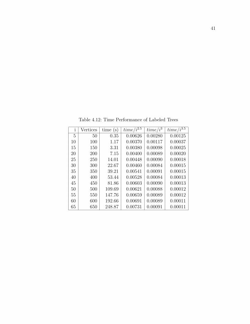
The number of labeled trees are shown in Table 4.11 and time used to obtain
these numbers are shown in Table 4.12. From Table 4.12, we can see that time/i3
seems to approach a constant. So, the time complexity for labeled trees could be
Θ(n3), or perhaps Θ(nc) for some constant c near 3.
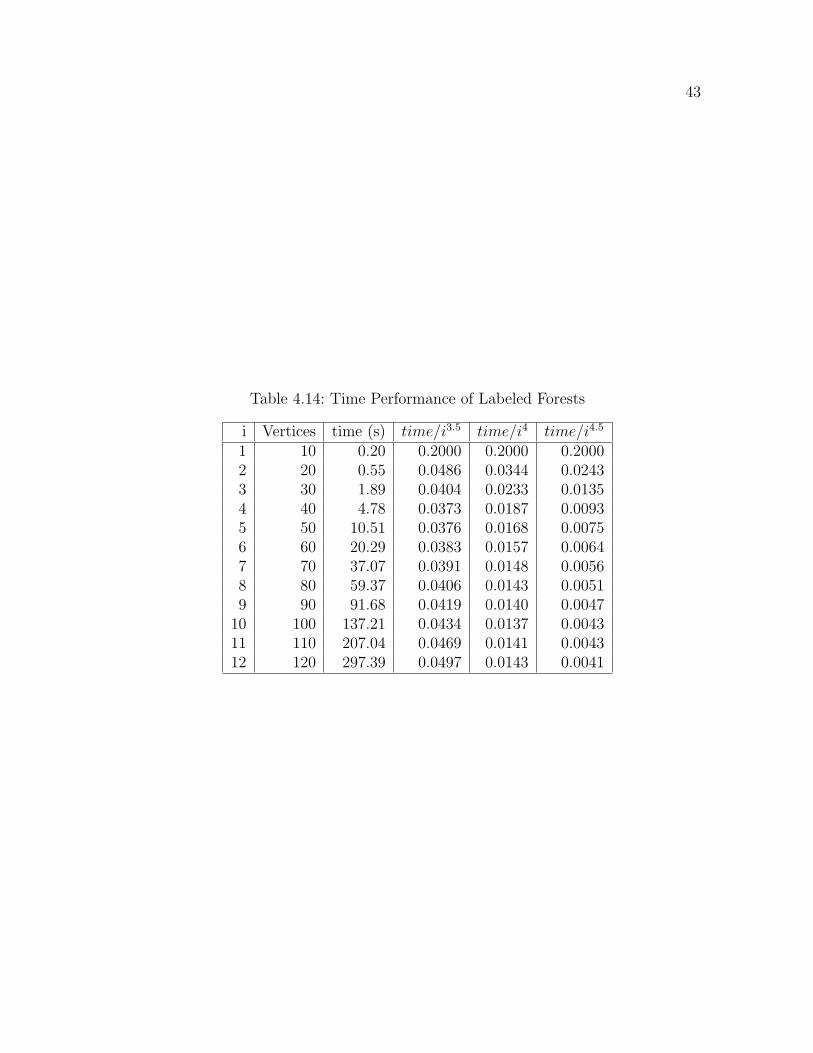
The number of labeled forests are shown in Table 4.13 and time performance
of labeled forests is shown in Table 4.14. From Table 4.14, we can see that time/i4
seems to approach a constant. So, the time complexity for labeled trees could be
Θ(n4), or perhaps Θ(nc) for some constant c near 4.
30
t(x) in def fact(x) in def
def t(x)
result.append(Ration())
result.append(Ration(1))
b=0L
for i in range(2, n):
a=i-2
b=power(i, a)
c=factorial(i)
d=Ration(b)/Ration(c)
result.append(d)
endef
def fact(x)
for i in range(n):
a=factorial(i)
result.append(Ration(a))
endef
begin
f(x) = e ^ t(x)
r(x) = f(x) @ fact(x)
r(x)

40
Table 4.11: Number of Labeled Trees
Vertices Labeled Trees0 01 12 13 34 165 1256 12967 168078 2621449 4782969
10 10000000011 235794769112 6191736422413 179216039403714 5669391237529615 194619506835937516 7205759403792793617 286242305150981579318 12143953109659425177619 548038685778480218593920 26214400000000000000000021 1324849664033102612558078122 70542949868640404420794777623 3947158412069548588724958962324 231551350147618771605743311257625 14210854715202003717422485351562526 910668576953721495679981403609497627 60826678771335770911968399261886130728 4227745295057828426348562277214873190429 3053134545970524535745336759489912159909
41
Table 4.12: Time Performance of Labeled Trees
i Vertices time (s) time/i2.5 time/i3 time/i3.5
5 50 0.35 0.00626 0.00280 0.0012510 100 1.17 0.00370 0.00117 0.0003715 150 3.31 0.00380 0.00098 0.0002520 200 7.15 0.00400 0.00089 0.0002025 250 14.01 0.00448 0.00090 0.0001830 300 22.67 0.00460 0.00084 0.0001535 350 39.21 0.00541 0.00091 0.0001540 400 53.44 0.00528 0.00084 0.0001345 450 81.86 0.00603 0.00090 0.0001350 500 109.69 0.00621 0.00088 0.0001255 550 147.76 0.00659 0.00089 0.0001260 600 192.66 0.00691 0.00089 0.0001165 650 248.87 0.00731 0.00091 0.00011

42
Table 4.13: Number of Labeled Forests
Vertices Labeled Forests0 11 12 23 74 385 2916 29327 369618 5619489 10026505
10 20560853611 476744067912 12337320320813 352563011010714 11028428300664015 374835769956096116 13755791009484084817 542117905035033492918 22835948733519457052819 1023920647304088127757520 48690974486257665428361621 2447669761084907491190037122 129692217032696701702145619223 7224234394625047476537521609724 422040860405279505063069393760025 25802582394869095934016499242300126 1647632513313120685638853134500083227 109688154302489879969077541547487671128 7600421771817836654284855610186632716829 5473008907162709455528258930972402876875
43
Table 4.14: Time Performance of Labeled Forests
i Vertices time (s) time/i3.5 time/i4 time/i4.5
1 10 0.20 0.2000 0.2000 0.20002 20 0.55 0.0486 0.0344 0.02433 30 1.89 0.0404 0.0233 0.01354 40 4.78 0.0373 0.0187 0.00935 50 10.51 0.0376 0.0168 0.00756 60 20.29 0.0383 0.0157 0.00647 70 37.07 0.0391 0.0148 0.00568 80 59.37 0.0406 0.0143 0.00519 90 91.68 0.0419 0.0140 0.0047
10 100 137.21 0.0434 0.0137 0.004311 110 207.04 0.0469 0.0141 0.004312 120 297.39 0.0497 0.0143 0.0041

Chapter 5
Applications of AutoGF to Counting Integer Partitions
Definition A partition of a positive integer n is a representation of n as a sum of
positive integers
n = r1 + r2 + · · ·+ rk,
where r1 ≥ r2 ≥ · · · ≥ rk ≥ 1. The numbers r1, r2, · · · , rk are the parts of the
partition and thus the above is a partition of n into k parts (Wilf 1990, p. 91).
There are 7 partitions of 5, namely 5 = 5, = 4+1, = 3+2, = 3+1+1, = 2+2+2, =
2 + 1 + 1 + 1, = 1 + 1 + 1 + 1 + 1. The number of partitions of n is denoted by p(n).
The following theorem describes the generating function of p(n) (Hall 1986, p. 34).
Theorem 5 The ordinary generating function of p(n),
P (x) = 1 + p(1)x + p(2)x2 + · · ·+ p(n)xn + · · ·
is given by
P (x) =∞∏
i=1
1
1− xi.
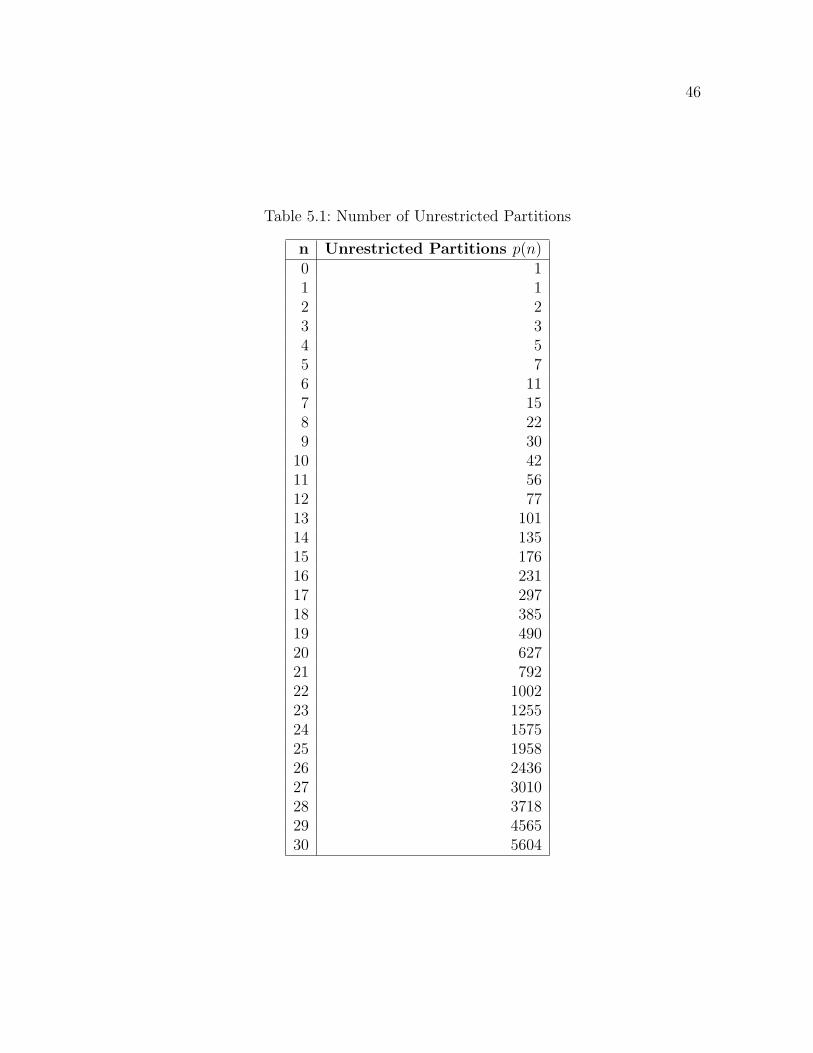
The text file below is used to calculate p(n) based on the theorem. The results
are shown in Table 5.1 and the time performance is in Table 5.2. From Table 5.2, we
can see that time/i3 seems roughly to approach a constant for unrestricted integer
partitions. So, the time complexity for unrestricted integer partitions could be Θ(n3),
or perhaps Θ(nc) for some constant c near 3.
44

45
31
A(x) in def B(x) = 1
def A(x)
coeff1=[]
coeff2=[]
for i in range(n):
coeff1.append(Ration())
coeff2.append(Ration())
result.append(Ration())
result[0]=Ration(1)
result[1]=Ration(-1)
i=2
while i<=30:
for l in range(n):
coeff1[l]=Ration()
coeff2[l]=Ration()
coeff2[0]=Ration(1)
coeff2[i]=Ration(-1)
for j in range(n):
coeff1[j]=result[j]
for a in range(n):
b=a+1
s=Ration()
for c in range(b):
s=s+coeff1[c]*coeff2[a-c]
result[a]=s
i=i+1
endef
begin
C(x) = B(x) / A(x)
C(x)
A partition is said to be into distinct parts if the parts are all different. There are
3 partitions into distinct parts of 5, namely 5 = 5, = 4 + 1, = 3 + 2. The generating
function for partitions into distinct parts is (Hall 1986, Chapter 4, Problem 3, p. 46)
D(x) =∞∏
i=1
(1 + xi).
The following text file is used to calculate the numbers of partitions into distinct
parts. The results are shown in Table 5.3 and the time performance is in Table
46
Table 5.1: Number of Unrestricted Partitions
n Unrestricted Partitions p(n)0 11 12 23 34 55 76 117 158 229 30
10 4211 5612 7713 10114 13515 17616 23117 29718 38519 49020 62721 79222 100223 125524 157525 195826 243627 301028 371829 456530 5604

47
Table 5.2: Time Performance of Unrestricted Partitions
i n time (s) time/i2.5 time/i3 time/i3.5
1 10 0.31 0.310 0.310 0.31002 20 1.38 0.244 0.173 0.12203 30 4.63 0.297 0.171 0.09904 40 10.08 0.315 0.158 0.07885 50 18.64 0.333 0.149 0.06676 60 32.46 0.368 0.150 0.06147 70 54.80 0.423 0.160 0.06048 80 73.82 0.408 0.144 0.05109 90 109.68 0.451 0.150 0.0502
10 100 147.06 0.465 0.147 0.046511 110 193.54 0.482 0.145 0.0438
5.4. From Table 5.4, we can see that time/i3 roughly approaches a constant for the
distinct integer partitions. So, the time complexity for distinct integer partitions
could be Θ(n3) or Θ(nc) for some constant c near 3.
31
A(x) in def
def A(x)
coeff1=[]
coeff2=[]
for i in range(n):
coeff1.append(Ration())
coeff2.append(Ration())
result.append(Ration())
result[0]=Ration(1)
result[1]=Ration(1)
i=2
while i <=30:
for l in range(n):
coeff1[l]=Ration()
coeff2[l]=Ration()
coeff2[0]=Ration(1)
coeff2[i]=Ration(1)

48
for j in range(n):
coeff1[j]=result[j]
for a in range(n):
b=a+1
s=Ration()
for c in range(b):
s=s+coeff1[c]*coeff2[a-c]
result[a]=s
i=i+1
endef
begin
A(x)

49
Table 5.3: Number of Partitions with Distinct Parts
n Partitions with Distinct Parts D(n)0 11 12 13 24 25 36 47 58 69 8
10 1011 1212 1513 1814 2215 2716 3217 3818 4619 5420 6421 7622 8923 10424 12225 14226 16527 19228 22229 25630 296

50
Table 5.4: Time Performance of Partitions into Distinct Parts
i n time (s) time/i2.5 time/i3 time/i3.5
1 10 0.36 0.36 0.36 0.362 20 1.35 0.239 0.169 0.1193 30 4.57 0.293 0.169 0.09774 40 9.87 0.308 0.154 0.07715 50 19.14 0.342 0.153 0.06846 60 32.24 0.366 0.149 0.06097 70 51.20 0.395 0.149 0.05648 80 77.13 0.426 0.151 0.05339 90 110.87 0.456 0.152 0.0507
10 100 152.57 0.482 0.153 0.048211 110 196.32 0.489 0.147 0.0445

Chapter 6
Conclusion
We have developed an automated system, AutoGF, to calculate coefficients of gener-
ating functions. The user of AutoGF must analyze the generating function problem
and express it as a series of operations on basic generating functions which are defined
in the system or supplied by the user. The user then creates a text file listing these
operations and passes the text file to AutoGF. In turn, AutoGF tokenizes and analyzes
the text file, computes the requested coefficients and writes them to an output file.
Exponential generating functions have been widely applied to count classes of
labeled graphs and digraphs. The numbers of graphs or digraphs with different
numbers of vertices can be found by applying the Hadamard product of the fac-
torial number series to the coefficients of exponential generating functions. In this
thesis, AutoGF is used to count the numbers of connected labeled graphs, labeled
blocks, connected labeled eulerian graphs, labeled acyclic digraphs, labeled strong
digraphs, and labeled forests. The time performances of these graph enumerations
are measured and their time complexities are estimated. The time complexities are
summarized in Table 6.1. The time used to count the number of graphs of a given
type is determined by the number of operations and time used for each operation.
The latter depends on the implementation of arithmetic operations and the size and
growth rate of the numbers. From Table 6.1, we can see that the time complexities
for these graph enumerations appear to lie in the range Θ(n4) to Θ(n5) except for
labeled trees. The latter seems to be in the class Θ(n3), presumably because it only
requires simple manipulations of numbers of size Θ(nlogn) instead of Θ(n2).
51

52
Table 6.1: Time Complexity of Graph Enumerations
Graphs Time ComplexityConnected Labeled Graph Θ(n4)
Labeled Blocks Θ(n5)Connected Labeled Eulerian Graph Θ(n4)
Labeled Acyclic Digraphs Θ(n5)Labeled Strong Digraphs Θ(n4)
Labeled Trees Θ(n3)Labeled Forests Θ(n4)
Table 6.2: Time Complexity of Integer Partition Enumerations
Partition Type Time ComplexityGeneral Partition Θ(n3)Distinct Partition Θ(n3)
Generating functions can also be used to count partitions of integers. In this
thesis, AutoGF is used to count general partitions and partitions into distinct parts.
Time complexities are estimated and summarized in Table 6.2. Both types of parti-
tions can apparently be counted in time complexity Θ(n3).
There are two obvious directions for future improvements to AutoGF. One would
be to allow for arbitrary polynomials with rational coefficients to be used as coef-
ficients of generating functions. At present, only generating functions with rational
coefficients can be calculated and manipulated by AutoGF. Arbitrary rational poly-
nomial coefficients would allow for applications in which there is more than one
parameter to keep track of, such as graphs or digraphs by numbers of edges or
numbers of components as well as by numbers of vertices.

53
The second direction would be to allow for problems defined implicitly by equa-
tions, which would then be automatically expressed in terms of fundamental opera-
tions on basic series.

Bibliography
D. M. Beazley, Python Essential Reference, 2nd ed., New Riders, Indianapolis, IN
(2001).
R. P. Brent and H. T. Kung, Fast Algorithms for Manipulating Formal Power
Series, J. Assoc. Comput. Mach. 25 (1978) 581-595.
R. L. Finney, M. D. Weir, and F. R. Giordano, Thomas’s Calculus, Part I, 10th
ed., Addison Wesley, Reading, MA (2000).
M. Hall, Jr., Combinatorial Theory, 2nd ed., John Wiley & Sons, New York (1986).
F. Harary and E. M. Palmer, Graphical Enumeration, Academic Press, New York
(1973).
D. E. Knuth, The Art of Computer Programming, Volume 2, Seminumerical Algo-
rithms, 3rd ed., Addison Wesley, Reading, MA (1998).
A. Lessa, Python Developer’s Handbook, Sams Publishing,Indianapolis, IN (2001).
R. W. Robinson, Counting Labeled Acyclic Digraphs, New Directions in the Theory
of Graphs (F. Harary, ed.) Academic Press, New York (1973) 239-273.
A. Tucker, Applied Combinatorics, 3rd ed., John Wiley & Sons, New York (1995).
D. B. West, Introduction to Graph Theory, Prentice Hall, Upper Saddle River, NJ
(1996).
H. S. Wilf, Generatingfunctionology, Academic Press, San Diego, CA (1990).
54