Embed Size (px)
Citation preview
AutoCAD® Map 3D 2010
Tutorials
April 2009

© 2009 Autodesk, Inc. All Rights Reserved. Except as otherwise permitted by Autodesk, Inc., this publication, or parts thereof, may not bereproduced in any form, by any method, for any purpose. Certain materials included in this publication are reprinted with the permission of the copyright holder. TrademarksThe following are registered trademarks or trademarks of Autodesk, Inc., in the USA and other countries: 3DEC (design/logo), 3December,3December.com, 3ds Max, ADI, Alias, Alias (swirl design/logo), AliasStudio, Alias|Wavefront (design/logo), ATC, AUGI, AutoCAD, AutoCADLearning Assistance, AutoCAD LT, AutoCAD Simulator, AutoCAD SQL Extension, AutoCAD SQL Interface, Autodesk, Autodesk Envision, AutodeskInsight, Autodesk Intent, Autodesk Inventor, Autodesk Map, Autodesk MapGuide, Autodesk Streamline, AutoLISP, AutoSnap, AutoSketch,AutoTrack, Backdraft, Built with ObjectARX (logo), Burn, Buzzsaw, CAiCE, Can You Imagine, Character Studio, Cinestream, Civil 3D, Cleaner,Cleaner Central, ClearScale, Colour Warper, Combustion, Communication Specification, Constructware, Content Explorer, Create>what's>Next>(design/logo), Dancing Baby (image), DesignCenter, Design Doctor, Designer's Toolkit, DesignKids, DesignProf, DesignServer, DesignStudio,Design|Studio (design/logo), Design Web Format, Discreet, DWF, DWG, DWG (logo), DWG Extreme, DWG TrueConvert, DWG TrueView, DXF,Ecotect, Exposure, Extending the Design Team, Face Robot, FBX, Filmbox, Fire, Flame, Flint, FMDesktop, Freewheel, Frost, GDX Driver, Gmax,Green Building Studio, Heads-up Design, Heidi, HumanIK, IDEA Server, i-drop, ImageModeler, iMOUT, Incinerator, Inferno, Inventor, InventorLT, Kaydara, Kaydara (design/logo), Kynapse, Kynogon, LandXplorer, LocationLogic, Lustre, Matchmover, Maya, Mechanical Desktop, Moonbox,MotionBuilder, Movimento, Mudbox, NavisWorks, ObjectARX, ObjectDBX, Open Reality, Opticore, Opticore Opus, PolarSnap, PortfolioWall,Powered with Autodesk Technology, Productstream, ProjectPoint, ProMaterials, RasterDWG, Reactor, RealDWG, Real-time Roto, REALVIZ,Recognize, Render Queue, Retimer,Reveal, Revit, Showcase, ShowMotion, SketchBook, Smoke, Softimage, Softimage|XSI (design/logo),SteeringWheels, Stitcher, Stone, StudioTools, Topobase, Toxik, TrustedDWG, ViewCube, Visual, Visual Construction, Visual Drainage, VisualLandscape, Visual Survey, Visual Toolbox, Visual LISP, Voice Reality, Volo, Vtour, Wire, Wiretap, WiretapCentral, XSI, and XSI (design/logo). The following are registered trademarks or trademarks of Autodesk Canada Co. in the USA and/or Canada and other countries:Backburner,Multi-Master Editing, River, and Sparks. The following are registered trademarks or trademarks of MoldflowCorp. in the USA and/or other countries: Moldflow, MPA, MPA(design/logo),Moldflow Plastics Advisers, MPI, MPI (design/logo), Moldflow Plastics Insight,MPX, MPX (design/logo), Moldflow Plastics Xpert. All other brand names, product names or trademarks belong to their respective holders. DisclaimerTHIS PUBLICATION AND THE INFORMATION CONTAINED HEREIN IS MADE AVAILABLE BY AUTODESK, INC. "AS IS." AUTODESK, INC. DISCLAIMSALL WARRANTIES, EITHER EXPRESS OR IMPLIED, INCLUDING BUT NOT LIMITED TO ANY IMPLIED WARRANTIES OF MERCHANTABILITY ORFITNESS FOR A PARTICULAR PURPOSE REGARDING THESE MATERIALS. Published by:Autodesk, Inc.111 Mclnnis ParkwaySan Rafael, CA 94903, USA

Contents
Chapter 1 Tutorial: Introducing AutoCAD Map 3D 2010 . . . . . . . . . . . 1Lesson 1: Get Ready to Use the Tutorials . . . . . . . . . . . . . . . . . . 1
Exercise 1: Prepare your sample data . . . . . . . . . . . . . . . . . 2Exercise 2: Save your tutorial maps . . . . . . . . . . . . . . . . . 3Exercise 3: Set up the tutorial window . . . . . . . . . . . . . . . . 3Exercise 4: Choose a workspace . . . . . . . . . . . . . . . . . . . 4
Lesson 2: Take a Quick Tour of AutoCAD Map 3D . . . . . . . . . . . . . 4The Ribbon . . . . . . . . . . . . . . . . . . . . . . . . . . . . . . 6Finding Commands . . . . . . . . . . . . . . . . . . . . . . . . . 9Workspaces . . . . . . . . . . . . . . . . . . . . . . . . . . . . . 11The Task Pane . . . . . . . . . . . . . . . . . . . . . . . . . . . . 12Properties Palette . . . . . . . . . . . . . . . . . . . . . . . . . . 20Data Table and Data View . . . . . . . . . . . . . . . . . . . . . . 21Status Bars . . . . . . . . . . . . . . . . . . . . . . . . . . . . . . 23Layout Tabs . . . . . . . . . . . . . . . . . . . . . . . . . . . . . 24Dynamic Input . . . . . . . . . . . . . . . . . . . . . . . . . . . 25Shortcut Menus . . . . . . . . . . . . . . . . . . . . . . . . . . . 28Options . . . . . . . . . . . . . . . . . . . . . . . . . . . . . . . 29
Lesson 3: Get Started . . . . . . . . . . . . . . . . . . . . . . . . . . . 30Exercise 1: Create a map . . . . . . . . . . . . . . . . . . . . . . 30Exercise 2: Use Data Connect to add data to your map . . . . . . 32Exercise 3: Style a feature . . . . . . . . . . . . . . . . . . . . . . 33Where you are now . . . . . . . . . . . . . . . . . . . . . . . . . 35
iii

Chapter 2 Tutorial: Building a Map . . . . . . . . . . . . . . . . . . . . . 37About the Building a Map Tutorial . . . . . . . . . . . . . . . . . . . . 37Lesson 1: Use Multiple Sources . . . . . . . . . . . . . . . . . . . . . . 38
Exercise 1: Drag and drop a source file . . . . . . . . . . . . . . . 38Exercise 2: Attach a drawing file . . . . . . . . . . . . . . . . . . 39Exercise 3: Query in data from the drawing . . . . . . . . . . . . 41Exercise 4: Use Data Connect . . . . . . . . . . . . . . . . . . . . 43Exercise 5: Add a raster image . . . . . . . . . . . . . . . . . . . . 45Exercise 6: Display the raster image behind other features . . . . . 47
Lesson 2: Style Map Features . . . . . . . . . . . . . . . . . . . . . . . 49Exercise 1: Create a theme for the parcels layer . . . . . . . . . . 49Exercise 2: Define the theme . . . . . . . . . . . . . . . . . . . . 50Exercise 3: Add labels . . . . . . . . . . . . . . . . . . . . . . . . 52
Lesson 3: Change the Display by Zoom Level . . . . . . . . . . . . . . 54Exercise 1: Add roads to your map . . . . . . . . . . . . . . . . . 55Exercise 2: Create a composite road style . . . . . . . . . . . . . . 56Exercise 3: View styles at different zoom levels . . . . . . . . . . . 59
Lesson 4: Create Map Features . . . . . . . . . . . . . . . . . . . . . . 60Exercise 1: Draw a new parcel . . . . . . . . . . . . . . . . . . . . 60Exercise 2: Add information about the new parcel . . . . . . . . . 62
Lesson 5: Find Objects . . . . . . . . . . . . . . . . . . . . . . . . . . . 63Exercise 1: Display the Data Table . . . . . . . . . . . . . . . . . 63Exercise 2: Filter the Data Table . . . . . . . . . . . . . . . . . . . 63
Lesson 6: Edit Objects . . . . . . . . . . . . . . . . . . . . . . . . . . . 65Exercise 1: Check out and edit a feature . . . . . . . . . . . . . . 65Exercise 2: Update information for the edited feature . . . . . . . 66
Lesson 7: Create a Legend . . . . . . . . . . . . . . . . . . . . . . . . . 67Exercise 1: Insert a legend object . . . . . . . . . . . . . . . . . . 67Exercise 2: Change the order of items in the legend . . . . . . . . 69
Lesson 8: Publish Your Map . . . . . . . . . . . . . . . . . . . . . . . . 70Exercise 1: Specify attributes to include . . . . . . . . . . . . . . 70Exercise 2: Publish to DWF . . . . . . . . . . . . . . . . . . . . . 72
Lesson 9: Branch Out - Find Data Sources . . . . . . . . . . . . . . . . 74Exercise 1: Explore the Data Portal - DigitalGlobe® . . . . . . . . 75Exercise 2: Explore the Data Portal - NAVTEQ™ . . . . . . . . . . 76Exercise 3: Explore the Data Portal - Intermap™ . . . . . . . . . . 76Exercise 4: Try out the sample data . . . . . . . . . . . . . . . . . 77
Chapter 3 Tutorial: Moving From AutoCAD to AutoCAD Map 3D . . . . . . 83About The AutoCAD/AutoCAD Map 3D Tutorial . . . . . . . . . . . . . 83Lesson 1: Prepare Drawings for Use With AutoCAD Map 3D . . . . . . 83
Exercise 1: Set up a drive alias . . . . . . . . . . . . . . . . . . . . 84Exercise 2: Georeference source drawings . . . . . . . . . . . . . 86
Lesson 2: Clean Up Your Drawings . . . . . . . . . . . . . . . . . . . . 89Exercise 1: Delete duplicates . . . . . . . . . . . . . . . . . . . . 90
iv | Contents
Exercise 2: Extend undershoots . . . . . . . . . . . . . . . . . . . 93Exercise 3: Use cleanup profiles (optional) . . . . . . . . . . . . . 96
Lesson 3: Add Drawing Objects to a Map . . . . . . . . . . . . . . . . 98Exercise 1: Attach source drawings . . . . . . . . . . . . . . . . . 99Exercise 2: Preview attached drawings with Quick View . . . . . 100Exercise 3: Preview drawing objects with a property query . . . . 102Exercise 4: Retrieve objects with a property and location
query . . . . . . . . . . . . . . . . . . . . . . . . . . . . . . . 105Exercise 5: Query object data . . . . . . . . . . . . . . . . . . . 108Exercise 6: Create an object data index (optional) . . . . . . . . 111
Lesson 4: Add Raster Images . . . . . . . . . . . . . . . . . . . . . . . 114Exercise 1: Insert a raster image . . . . . . . . . . . . . . . . . . 114Exercise 2: View image information . . . . . . . . . . . . . . . . 117Exercise 3: Change the display order . . . . . . . . . . . . . . . 119
Lesson 5: Modify Raster Images . . . . . . . . . . . . . . . . . . . . . 120Exercise 1: Adjust image brightness, contrast, and fade . . . . . . 120Exercise 2: Clip the image . . . . . . . . . . . . . . . . . . . . . 122Exercise 3: Add a raster image to a Display Manager layer . . . . 125
Lesson 6: Share Your Map with Others . . . . . . . . . . . . . . . . . 127Exercise 1: Export a map to Autodesk SDF . . . . . . . . . . . . 128Exercise 2: Publish a map to a DWF file . . . . . . . . . . . . . . 130
Chapter 4 Tutorial: Classifying Drawing Objects . . . . . . . . . . . . . . 135About the Classifying Drawing Objects Tutorial . . . . . . . . . . . . 135Lesson 1: Set Up For Classification . . . . . . . . . . . . . . . . . . . 136
Exercise 1: Set up your work environment . . . . . . . . . . . . 137Exercise 2: Set up your user privileges . . . . . . . . . . . . . . . 137
Lesson 2: Define Object Classes . . . . . . . . . . . . . . . . . . . . . 139Exercise 1: Create the object class definition file . . . . . . . . . 139Exercise 2: Define an object class . . . . . . . . . . . . . . . . . 140Exercise 3: Add object classes to the definition file . . . . . . . . 147
Lesson 3: Classify Objects . . . . . . . . . . . . . . . . . . . . . . . . 148Exercise 1: Classify the signal objects . . . . . . . . . . . . . . . 148Exercise 2: Classify roads and parcels . . . . . . . . . . . . . . . 152
Lesson 4: Create a Map Using Object Classes . . . . . . . . . . . . . . 153Exercise 1: Create a map . . . . . . . . . . . . . . . . . . . . . . 154Exercise 2: Assign a coordinate system . . . . . . . . . . . . . . 156Exercise 3: Query in objects . . . . . . . . . . . . . . . . . . . . 158
Lesson 5: Create and Edit Objects Using Object Classes . . . . . . . . 159Exercise 1: Create objects using object classes . . . . . . . . . . . 159Exercise 2: Edit classified objects . . . . . . . . . . . . . . . . . 162
Lesson 6: Generate Metadata for a Classified Drawing . . . . . . . . . 165Exercise 1: View metadata . . . . . . . . . . . . . . . . . . . . . 165Exercise 2: Share metadata . . . . . . . . . . . . . . . . . . . . . 166
Lesson 7: Use Object Classes When Exporting . . . . . . . . . . . . . 168Exercise 1: Export object classes to SDF . . . . . . . . . . . . . . 168
Contents | v

Exercise 2: Connect to the resulting SDF file . . . . . . . . . . . 170Exercise 3: Style the new feature classes . . . . . . . . . . . . . . 172
Object Classification: Best Practices . . . . . . . . . . . . . . . . . . . 174
Chapter 5 Tutorial: Creating a Map Book With an Inset . . . . . . . . . . 175About the Map Book Tutorial . . . . . . . . . . . . . . . . . . . . . . 175Lesson 1: Prepare the Map . . . . . . . . . . . . . . . . . . . . . . . . 175
Exercise 1: Create a map . . . . . . . . . . . . . . . . . . . . . . 176Exercise 2: Add data to your map . . . . . . . . . . . . . . . . . 176
Lesson 2: Customize a Map Book Template . . . . . . . . . . . . . . . 178Exercise 1: Change the printer/plotter for the template . . . . . 178Exercise 2: Resize the main viewport . . . . . . . . . . . . . . . 180Exercise 3: Modify the title block . . . . . . . . . . . . . . . . . 182Exercise 4: Replace the north arrow block . . . . . . . . . . . . . 185
Lesson 3: Create A Map Book . . . . . . . . . . . . . . . . . . . . . . 186Exercise 1: Create a key map view and a legend . . . . . . . . . . 186Exercise 2: Specify the map book settings . . . . . . . . . . . . . 187Exercise 3: Preview and generate the map book . . . . . . . . . . 189
Lesson 4: Create an Inset . . . . . . . . . . . . . . . . . . . . . . . . . 193Exercise 1: Draw a viewport for the inset . . . . . . . . . . . . . 193Exercise 2: Change the information displayed in the
viewport . . . . . . . . . . . . . . . . . . . . . . . . . . . . . 194Lesson 5: Publish The Map Book . . . . . . . . . . . . . . . . . . . . 195
Exercise 1: Set DWF publishing options . . . . . . . . . . . . . . 196Exercise 2: Set background publishing options . . . . . . . . . . 197Exercise 3: Publish the map book to DWF format . . . . . . . . . 198
Chapter 6 Tutorial: Analyzing Data . . . . . . . . . . . . . . . . . . . . . 201About the Analyzing Data Tutorial . . . . . . . . . . . . . . . . . . . 201Lesson 1: Analyze Data Visually, Using Surfaces . . . . . . . . . . . . 202
Exercise 1: Prepare your map file . . . . . . . . . . . . . . . . . 202Exercise 2: Add a surface to view elevation data . . . . . . . . . 204Exercise 3: Add a layer on top of the surface . . . . . . . . . . . 209Exercise 4: Drape a parcel layer on top of the surface . . . . . . . 212
Lesson 2: Analyze Data With External Information Using Joins . . . . 214Exercise 1: Set up an ODBC connection for an Access database
. . . . . . . . . . . . . . . . . . . . . . . . . . . . . . . . . . 215Exercise 2: Connect to the Access database . . . . . . . . . . . . 217Exercise 3: Join the data from the ODBC source to the layer
containing the parcels . . . . . . . . . . . . . . . . . . . . . . 218Exercise 4: Use the joined data for calculated fields and
styles . . . . . . . . . . . . . . . . . . . . . . . . . . . . . . . 219Lesson 3: Analyze Data by Proximity Using Buffers . . . . . . . . . . . 220
Exercise 1: Create a buffer representing a constructionzone . . . . . . . . . . . . . . . . . . . . . . . . . . . . . . . 221
vi | Contents
Exercise 2: Select the parcels within the construction-zonebuffer . . . . . . . . . . . . . . . . . . . . . . . . . . . . . . . 222
Exercise 3: Export the construction-zone parcels to an SDFfile . . . . . . . . . . . . . . . . . . . . . . . . . . . . . . . . 224
Exercise 4: Compare the two parcel layers . . . . . . . . . . . . . 225Exercise 5: Export the data to CSV for use in a report . . . . . . . 228
Lesson 4: Perform a Flood Analysis with Overlay . . . . . . . . . . . . 229Exercise 1: Add the layers to compare . . . . . . . . . . . . . . . 230Exercise 2: Use an overlay to compare two layers . . . . . . . . . 231Exercise 3: Add and style a road layer . . . . . . . . . . . . . . . 234Exercise 4: Add emergency response points . . . . . . . . . . . . 236Exercise 5: Find streets that are far from a hospital . . . . . . . . 237
Lesson 5: Automate an Overlay Operation with a Workflow . . . . . . 239Exercise 1: Edit a workflow . . . . . . . . . . . . . . . . . . . . 239Exercise 2: Complete the workflow definition . . . . . . . . . . 243Exercise 3: Run the workflow . . . . . . . . . . . . . . . . . . . 244
Chapter 7 Tutorial: Managing Data From Different Sources . . . . . . . . 247About the Managing Data Tutorial . . . . . . . . . . . . . . . . . . . 247Lesson 1: Convert Drawing Layers to Feature Classes . . . . . . . . . . 250
Exercise 1: Examine the original drawing layers . . . . . . . . . 251Exercise 2: Examine the object data . . . . . . . . . . . . . . . . 253Exercise 3: Export the drawing layers to SDF - Select the
layers . . . . . . . . . . . . . . . . . . . . . . . . . . . . . . . 255Exercise 4: Export the drawing layers to SDF - Map object data
to feature class properties . . . . . . . . . . . . . . . . . . . . 256Exercise 5: Export the drawing layers to SDF - Map drawing
properties to feature class properties . . . . . . . . . . . . . . . 259Exercise 6: Export the drawing layers to SDF - Set export
options . . . . . . . . . . . . . . . . . . . . . . . . . . . . . . 262Lesson 2: Use the Resulting SDF Files . . . . . . . . . . . . . . . . . . 262
Exercise 1: Create a map . . . . . . . . . . . . . . . . . . . . . 263Exercise 2: Connect to the new SDF data . . . . . . . . . . . . . 264Exercise 3: Edit the schema . . . . . . . . . . . . . . . . . . . . 267Exercise 4: Add a property . . . . . . . . . . . . . . . . . . . . . 268Exercise 5: Populate the new property with values . . . . . . . . 271
Lesson 3: Move SDF Data to a Different Geospatial Format . . . . . . . 272Exercise 1: Connect to a new SHP file folder . . . . . . . . . . . 272Exercise 2: Use Bulk Copy to move an SDF layer to SHP
format . . . . . . . . . . . . . . . . . . . . . . . . . . . . . . 273Lesson 4: Import SDF Files as DWG Layers . . . . . . . . . . . . . . . 276
Exercise 1: Create a template for the imported material . . . . . 276Exercise 2: Import the SDF layers . . . . . . . . . . . . . . . . . 277Exercise 3: Use display layers to assign object properties . . . . . 279
Contents | vii
Chapter 8 Tutorial: Working with Polygon Features . . . . . . . . . . . . 283About the Polygon Features Tutorial . . . . . . . . . . . . . . . . . . 283Lesson 1: Connect to Parcel Data . . . . . . . . . . . . . . . . . . . . 284
Exercise 1: Create a map . . . . . . . . . . . . . . . . . . . . . 284Exercise 2: Bring in the parcel data . . . . . . . . . . . . . . . . 285
Lesson 2: Split a Polygon Feature . . . . . . . . . . . . . . . . . . . . 286Exercise 1: Define split/merge rules . . . . . . . . . . . . . . . . 286Exercise 2: Find the parcel to split . . . . . . . . . . . . . . . . . 288Exercise 3: Split the parcel . . . . . . . . . . . . . . . . . . . . . 290Exercise 4: Examine the results . . . . . . . . . . . . . . . . . . 291
Lesson 3: Use Joined Data to Create Calculated Properties . . . . . . . 292Exercise 1: Set up an ODBC connection for a Microsoft Access
database . . . . . . . . . . . . . . . . . . . . . . . . . . . . . 293Exercise 2: Connect to the Microsoft Access database . . . . . . 294Exercise 3: Join the ODBC data to the Parcels layer . . . . . . . . 295Exercise 4: Save the properties to a new data store . . . . . . . . 296Exercise 5: Create a calculated property . . . . . . . . . . . . . . 299
Lesson 4: Theme Polygon Features . . . . . . . . . . . . . . . . . . . 301Exercise 1: Create a theme . . . . . . . . . . . . . . . . . . . . . 301Exercise 2: Add labels that use an expression . . . . . . . . . . . 303
Lesson 5: Publish Your Styled Map to MapGuide . . . . . . . . . . . . 305Exercise 1: Publish to MapGuide . . . . . . . . . . . . . . . . . 305
Chapter 9 Glossary . . . . . . . . . . . . . . . . . . . . . . . . . . . . . 309
Index . . . . . . . . . . . . . . . . . . . . . . . . . . . . . . . 317
viii | Contents

Tutorial: IntroducingAutoCAD Map 3D 2010
■ These tutorials provide an overview of the product and hands-on exercises to help youlearn many aspects of AutoCAD Map 3D.
Lesson 1: Get Ready to Use the TutorialsThese AutoCAD Map 3D tutorials cover the following:
■ Introducing AutoCAD Map 3D 2010 (page 1): Take a quick tour of theapplication. Create a map file, assign a coordinate system, connect to data,style features, and save your work.
■ Building a map (page 37): Learn all the basics of creating a map from startto finish. Use multiple sources, design themes and composite styles to changethe appearance of objects, create new features and edit them, and publishyour finished map.
■ Moving from AutoCAD to AutoCAD Map 3D 2010 (page 83): Preparedrawings for use with AutoCAD Map 3D, clean up drawing data, add drawingobjects to a map, add and edit raster images, and share maps with others.
■ Classifying Drawing Objects (page 135): Define object classes, assign drawingobjects to different classes, and then use the object classes to create, edit,and export drawing objects. To be part of the object class, drawing objectsmust meet certain rules when they are classified. Object classes help to ensurethat drawing objects are standardized.
■ Creating a Map Book With an Inset (page 175): Customize a map booktemplate, create a map book, create an inset, and publish to DWF.
1
1
■ Analyzing Data (page 201): Add a surface and style it using a theme andcontour lines to show elevation. Join an external database to a feature andcreate a style using both sets of data. Create a buffer zone that highlightsareas within 1000 feet of a river and identify parcels that lie within thatzone. Export comma-separated data to use in a report to the owners ofthose parcels. Overlay two geospatial layers and save the resultingcomparison layer as a separate data store. Automate the overlay processwith a workflow.
■ Managing Data From Different Sources (page 247): Export drawing objectsto Autodesk SDF format, and then connect to the resulting SDF file to addit as a layer in another map. Use Bulk Copy to copy the SDF data to SHPformat. Import the SDF data to convert it back to drawing layers.
■ Working With Polygon Features (page 283): Connect to geospatial data forparcel polygons. Join a data source to the parcels to add assessor data. Adda new calculated property that uses native and joined properties. Split aparcel into two uneven pieces using the Split command and assignattributes to each resulting parcel using split/merge rules.
Exercise 1: Prepare your sample dataWhen you installed AutoCAD Map 3D, the tutorial sample data was installedon your computer in the \Program Files\AutoCAD Map 3D 2010\Help\Map 3DTutorials folder. You need that sample data to use the tutorials.
Copy the Map 3D Tutorials folder to My Documents. That way, if you changethe sample files, the original versions remain unchanged and can be usedagain and again.
To make a copy of the sample data
1 In Windows Explorer, navigate to the\Program Files\AutoCAD Map 3D2010\Help folder.
2 Right-click the Map 3D Tutorials folder and click Copy.
3 Navigate to your My Documents folder.
NOTE The location of My Documents varies, depending on your operatingsystem. For Microsoft Windows XP, it is usually C:\MyDocuments. For MicrosoftVista, it might be C:\Documents and Settings\Administrator\My Documents\Map3D Tutorials.
2 | Chapter 1 Tutorial: Introducing AutoCAD Map 3D 2010
4 Paste the Map 3D Tutorials folder into My Documents.
A new folder is displayed in My Documents, for example C:\MyDocuments\Map 3D Tutorials.
5 Add the location to the Favorites list in Windows Explorer, or make anote of it.
Exercise 2: Save your tutorial mapsYou can create a folder for any map files you create or change as you use thetutorials.
To create a folder for your tutorial map files
1 Open Windows Explorer.
2 Navigate to the C:\My Documents folder.
NOTE The location of My Documents varies, depending on your operatingsystem. For Microsoft Windows XP, it is usually C:\MyDocuments. For MicrosoftVista, it might be C:\Documents and Settings\Administrator\My Documents\Map3D Tutorials.
3 Click File ➤ New Folder.
4 Change the name of the new folder to My AutoCAD Map 3D Tutorial Data.
Exercise 3: Set up the tutorial windowResize the window that displays the tutorial instructions so you can see itwhile you work.
To resize the tutorial window
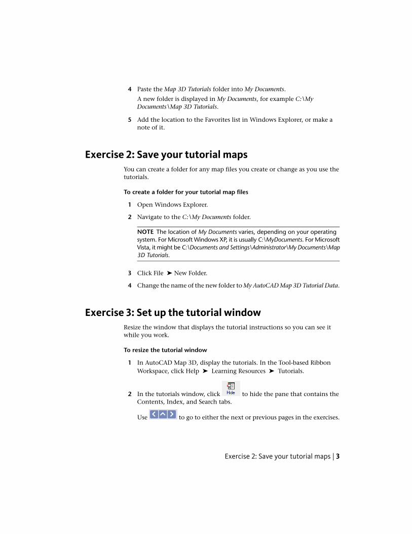
1 In AutoCAD Map 3D, display the tutorials. In the Tool-based RibbonWorkspace, click Help ➤ Learning Resources ➤ Tutorials.
2 In the tutorials window, click to hide the pane that contains theContents, Index, and Search tabs.
Use to go to either the next or previous pages in the exercises.
Exercise 2: Save your tutorial maps | 3

Exercise 4: Choose a workspaceThe tutorials assume that you are using the Tool-based Ribbon workspace (thedefault) unless otherwise noted.
To switch to the Tool-based Ribbon workspace
1 Click the workspace entry in the status bar.
2 Click Tool-based Ribbon Workspace.
Lesson 2: Take a Quick Tour of AutoCAD Map 3DStart by becoming familiar with the AutoCAD Map 3D window:
4 | Chapter 1 Tutorial: Introducing AutoCAD Map 3D 2010

The AutoCAD Map 3D window
To tour the AutoCAD Map 3D application window
1 Before you begin the tutorial, see Lesson 1: Get Ready to Use the Tutorials(page 1).
2 From the desktop or the Start menu, start AutoCAD Map 3D.
3 Click .
4 Navigate to the folder in My Documents where you copied the samplefiles.
5 Open SampleMap.dwg.
An alert may tell you that an undefined drive alias (page 311) is referenced.If so, click Define and use the following procedure. If not, proceed to“The Ribbon (page 6).”
To define a drive alias
■ The alias you need is already selected. Click in the Actual Path fieldand click Browse.
Lesson 2: Take a Quick Tour of AutoCAD Map 3D | 5

■ Navigate to the folder where you copied the sample files. Open thatfolder and click OK. (Be careful to select the Map 3D Tutorials subfolder,not the parent My Documents folder.)
■ Click Add, and then click Close.The sample data location is now mapped to your drive alias. In future,you can open the sample data without defining any further aliases.
The RibbonIn AutoCAD Map 3D, the tabs across the top of the application window arecalled a ribbon.
Tabs are like horizontal menus. Click a tab to see the commands associatedwith it. Sets of related commands are grouped in panels. Click a commandicon within a panel to select that command. Panel titles that display a downarrow contain more options. Panel titles that display an arrow in the lowerright corner have a dialog box associated with them.
Use the following techniques when working with the ribbon
■ To see more options for a panel, click the down arrow on the panel titlebar. Click the pushpin icon to keep the expanded portion displayed.For example, on the Home tab, click the down arrow on the Data panel.
■ To see the dialog box associated with a panel, click the arrow in the lowerright corner of the panel.For example, click the arrow on the Data panel to see the AutoCAD Map3D Options dialog box.
■ To see the keyboard shortcuts for displaying ribbon elements, press theAlt key. Press it again to hide the shortcuts.
■ To make a panel into a floating panel, drag its title bar away from theribbon. To reinsert it into the ribbon, drag it by its title bar to the desiredlocation.
■ To change the order of the tabs, drag a tab to a new position in the ribbon.
6 | Chapter 1 Tutorial: Introducing AutoCAD Map 3D 2010

■ To see commands for a particular Display Manager layer or Map Explorerentry, select that item. The ribbon expands to include a new tab for theselected item.By default, the ribbon switches to the new tab. To keep the ribbon fromswitching, at the Command prompt, type ribboncontextselect.
The application menu
The application menu includes the Search Field (page 10) and file-relatedcommands. Options displays the AutoCAD Options dialog box, which controlssuch things as the background color for maps.
To use the application menu
1 Click to see the application menu.
The Ribbon | 7

2 Do any of the following:
■ Click a command or submenu item on the left side of the applicationmenu.
■ To issue a different command, type its name into the Search field. SeeFinding Commands (page 9).
■ To switch between viewing recent documents and open documents,click the icons above the list of commands on the left.You can view recent documents as an ordered list, or by size, type, oraccess date. You can display large or small icons or images for eitherlist.
■ To change AutoCAD settings, click Options. See Options (page 29).
Quick Access Toolbar
Put the commands you use most often on the Quick Access Toolbar. You candisplay the toolbar at the top of the application window or just below theribbon.
To customize the Quick Access Toolbar
1 Click the down arrow next to the current Quick Access Toolbar.
2 Do any of the following:
■ To add a command to the Quick Access Toolbar, select any commandthat is listed.
■ To remove a selected command from the Quick Access Toolbar, clickit to clear its check mark.
■ To move the Quick Access Toolbar below the ribbon area, select ShowBelow The Ribbon.
To continue this tour of AutoCAD Map 3D, go to Finding Commands (page9)
See also:
■ Customizing Your Work Environment
■ Workspaces (page 11)
■ Finding Commands (page 9)
8 | Chapter 1 Tutorial: Introducing AutoCAD Map 3D 2010

Finding CommandsIf you know the command you want but cannot locate it in the ribbon, usethese tools to find it.
Ribbon Command Locator
The Ribbon Command Locator displays the current ribbon location for menucommands you used in previous releases of AutoCAD Map 3D. If the commandis not on the ribbon, the Ribbon Command Locator tells you how to accessit.
To locate a command on the ribbon
1 In the InfoCenter field, type the name of the command.
2 In the list that displays, choose Find A Command On The Ribbon.
NOTE You can also click Tools tab ➤ Customization panel ➤ RibbonCommand Locator.
3 In the Ribbon Command Locator window, specify the workspace youused in the previous release.
4 Select the command from a menu to see its current ribbon location (oran alternative way to access it).
Choose the command from the menu you used in the previous release of AutoCADMap 3D. Its current location appears in the Location In Ribbon field.
Finding Commands | 9

Search Field
Type a command name into the application menu Search field to issue thatcommand or display its dialog box.
The Search field is at the top of the application menu.
To use the Search field
1 Click to see the application menu.
2 In the field at the top of the menu, type all or part of the command name.
For example, type define. Commands beginning with the word “define”are displayed.
3 In the list that displays, click the appropriate entry.
10 | Chapter 1 Tutorial: Introducing AutoCAD Map 3D 2010
For example, if you typed define, click Define Query to display the DefineQuery Of Attached Drawing(s) dialog box.
NOTE If you customized the ribbon, the command might not be in theindicated location. To find its current location, use the Ribbon CommandLocator instead.
To continue this tour of AutoCAD Map 3D, go to Workspaces (page 11)
WorkspacesAutoCAD Map 3D comes with predefined workspaces. Each workspaceorganizes and displays commands and toolbars differently. You can switchbetween the following workspaces:
■ Tool-based ribbon workspace — customized for those who are alreadyfamiliar with the AutoCAD ribbon
■ Task-based ribbon workspace — customized for AutoCAD Map 3Dcommands
■ Map Classic — the menu-driven interface from earlier versions of theproduct. Many new commands are unavailable from this workspace.
You can customize any workspace, specifying the contents of the ribbon tabs,keyboard shortcuts, and how the mouse buttons behave.
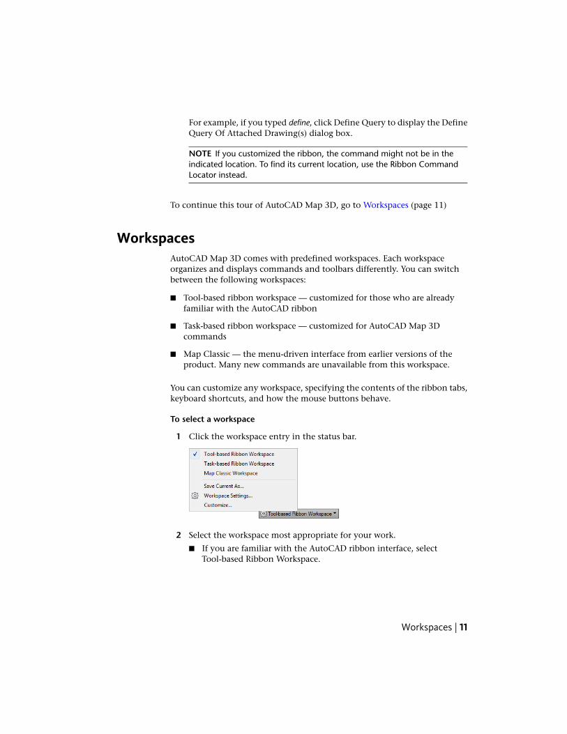
To select a workspace
1 Click the workspace entry in the status bar.
2 Select the workspace most appropriate for your work.
■ If you are familiar with the AutoCAD ribbon interface, selectTool-based Ribbon Workspace.
Workspaces | 11

The tutorials assume that you use the Tool-based Ribbon workspaceunless otherwise noted.
■ If you work mainly with AutoCAD Map 3D, select Task-based RibbonWorkspace.
■ Those familiar with older versions of AutoCAD Map 3D might preferMap Classic. However, commands added in recent releases are notavailable from the menus in this workspace.
To continue this tour of AutoCAD Map 3D, go to The Task Pane (page 12)
See also:
■ Customizing Your Work Environment
■ Finding Commands (page 9)
■ The Ribbon (page 6)
The Task PaneThe Task pane gives you quick access to frequently used features, and groupsthese features into task-related views. Use the Task pane to create, manage,display, and publish maps.
12 | Chapter 1 Tutorial: Introducing AutoCAD Map 3D 2010
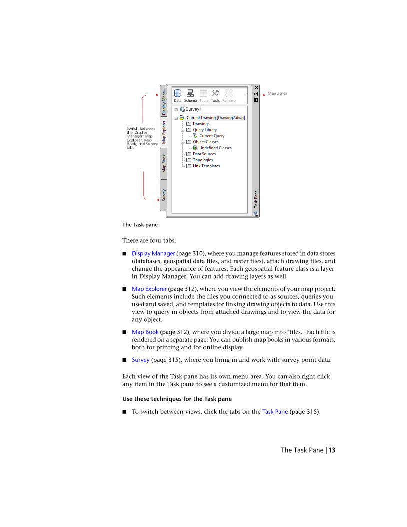
The Task pane
There are four tabs:
■ Display Manager (page 310), where you manage features stored in data stores(databases, geospatial data files, and raster files), attach drawing files, andchange the appearance of features. Each geospatial feature class is a layerin Display Manager. You can add drawing layers as well.
■ Map Explorer (page 312), where you view the elements of your map project.Such elements include the files you connected to as sources, queries youused and saved, and templates for linking drawing objects to data. Use thisview to query in objects from attached drawings and to view the data forany object.
■ Map Book (page 312), where you divide a large map into "tiles." Each tile isrendered on a separate page. You can publish map books in various formats,both for printing and for online display.
■ Survey (page 315), where you bring in and work with survey point data.
Each view of the Task pane has its own menu area. You can also right-clickany item in the Task pane to see a customized menu for that item.
Use these techniques for the Task pane
■ To switch between views, click the tabs on the Task Pane (page 315).
The Task Pane | 13
■ To see options for the current Task pane tab, click an icon in the menuarea at the top of the Task pane.
■ To hide the Task pane, click its Minimize button. Hold your cursor overthe Task pane title bar to see the Minimize button. To display the Taskpane after hiding it, move your cursor over its title bar.
■ To make the Task pane a floating palette, grab its title bar and drag it tothe desired location. Drag the title bar to a window edge to dock it again.
NOTE To minimize the Task pane each time you move your cursor away fromit, right-click the Task pane title bar and turn on Auto-hide.
■ To close the Task pane, click the X in its top right corner. Hold your cursorover the Task pane title bar to see the X.Once you have closed the Task pane, you can redisplay it. In the Tool-basedRibbon Workspace, click View tab ➤ Palettes panel ➤ Map Task pane.
See also:
■ Setting Task Pane Options
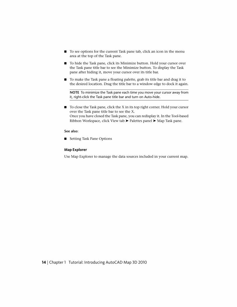
Map Explorer
Use Map Explorer to manage the data sources included in your current map.
14 | Chapter 1 Tutorial: Introducing AutoCAD Map 3D 2010
Use Map Explorer to manage the following:
■ feature sources (such as Oracle, ArcSDE, SHP, and SDF)
■ attached source drawings
■ drawing queries
■ object classes
■ external data sources for drawing objects
■ topologies
■ link templates
To attach a drawing to the current map
■ Drag the file from Windows Explorer to the Map Explorer tab of the Taskpane.
The Task Pane | 15
To use a database in a drawing
Do one of the following:
■ From Windows Explorer, drag a database file to the Map Explorer tab ofthe Task pane.If the Map Explorer tab does not immediately display the data source,right-click a blank space in the Map Explorer tab. Click Refresh.
■ Right-click the Data Sources folder on the Map Explorer tab and selectAttach.AutoCAD Map 3D automatically creates the required files forcommunicating with the database application. However, for some databasetypes, you must configure these files yourself.
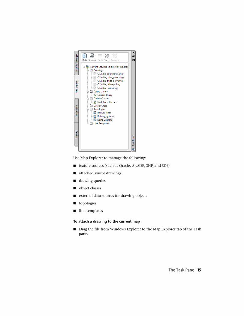
Display Manager
The Display Manager lets you create display maps. Each display map containsa set of styled layers. You can have more than one display map in a map file,and you can style the same data differently in each one.
Use Data Connect to add features to your map, or drag data sources into DisplayManager to add them as layers. For example, drag an SDF file from Windows®
Explorer into the layer area to add it.
16 | Chapter 1 Tutorial: Introducing AutoCAD Map 3D 2010

Use these techniques in the Display Manager
■ To change the appearance of a layer, select it and click .
■ To view and edit the attributes for a layer, select it and click
■ To change the draw order of the layers, select a layer and click Groups ➤
Draw Order. Drag the layers into the order in which you want them toappear in your map.
■ To see options specific to a layer, right-click any layer.Selecting a layer also displays a contextual tab in the ribbon, with theavailable options for that layer. See Shortcut Menus (page 28)
To use the Style Editor to style geospatial features
1 In the SampleMap.dwg file, select the Parcels layer in Display Manager(page 310).
2 To change the color of the parcels, click the Style button in the Task Pane(page 315) menu area.
■ Click in the Style field in the middle of the Style Editor window.
■ Select a different Foreground color and click OK.
■ Close the Style Editor by clicking the X in its top right corner. Thechanges are displayed in your map.
See also:
■ Overview of the Display Manager
■ Organizing Layers in Your Map
■ Controlling Display Order
Map Book
Use the Map Book tab to create printed maps, map books, and multi-pageDWFs from styled maps. Map Book uses the AutoCAD Sheet Set Manager, andprovides a tree view of the tiles in the map book, like pages in an atlas. Usenavigation arrows to move between tiles in your map.
The Task Pane | 17
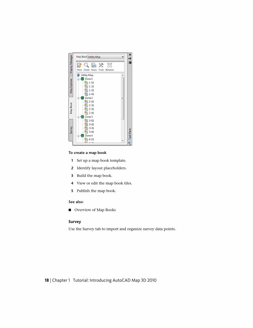
To create a map book
1 Set up a map book template.
2 Identify layout placeholders.
3 Build the map book.
4 View or edit the map book tiles.
5 Publish the map book.
See also:
■ Overview of Map Books
Survey
Use the Survey tab to import and organize survey data points.
18 | Chapter 1 Tutorial: Introducing AutoCAD Map 3D 2010

Use the Survey tab to import andorganize survey data.
To work with survey data
1 Create a survey data store to contain the data.
2 Import data from LandXML or ASCII files.
3 Organize the data:
■ Organize the data into projects.
■ Within each project, create surveys and classify points into pointgroups.
■ Create new points within defined point groups, and create featuresfrom points.
To continue this tour of AutoCAD Map 3D, go to Properties Palette (page 20)
See also:
■ Bringing in Survey Data
■ Working with Survey Data
The Task Pane | 19
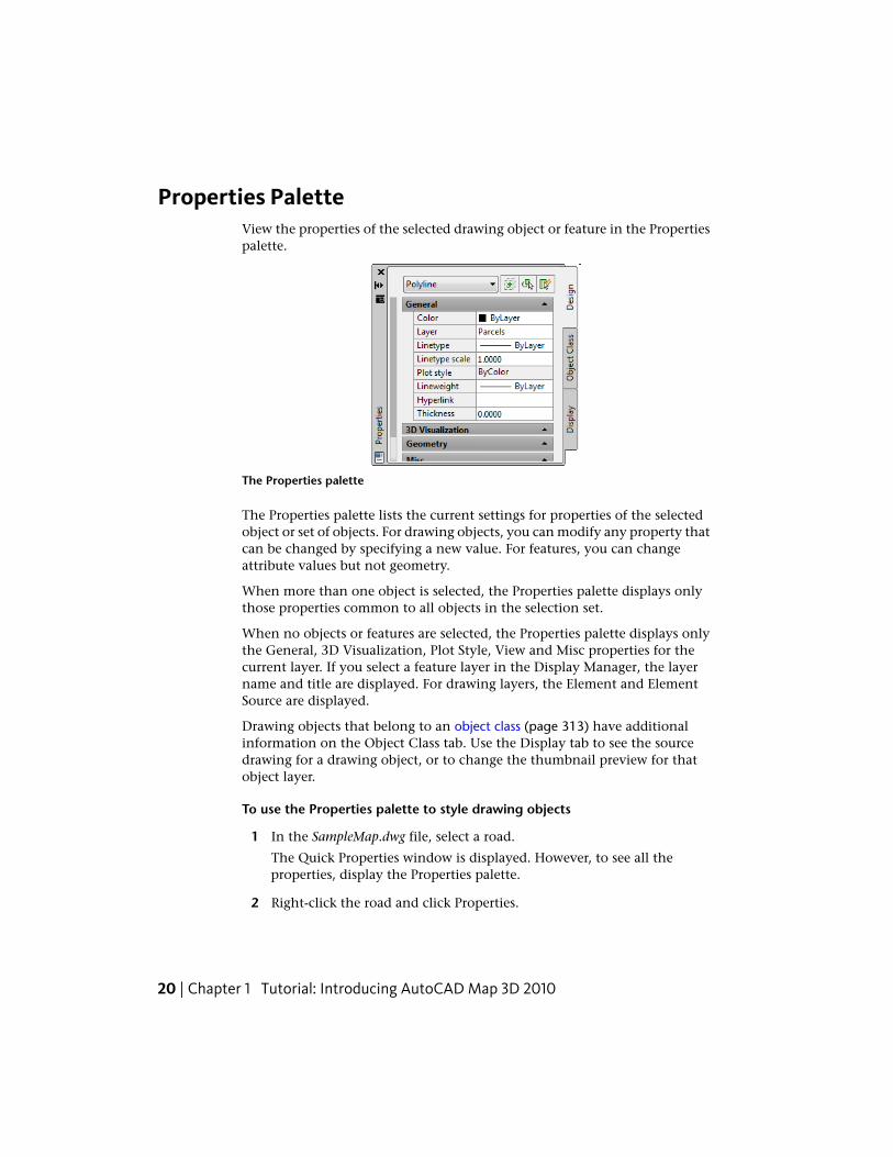
Properties PaletteView the properties of the selected drawing object or feature in the Propertiespalette.
The Properties palette
The Properties palette lists the current settings for properties of the selectedobject or set of objects. For drawing objects, you can modify any property thatcan be changed by specifying a new value. For features, you can changeattribute values but not geometry.
When more than one object is selected, the Properties palette displays onlythose properties common to all objects in the selection set.
When no objects or features are selected, the Properties palette displays onlythe General, 3D Visualization, Plot Style, View and Misc properties for thecurrent layer. If you select a feature layer in the Display Manager, the layername and title are displayed. For drawing layers, the Element and ElementSource are displayed.
Drawing objects that belong to an object class (page 313) have additionalinformation on the Object Class tab. Use the Display tab to see the sourcedrawing for a drawing object, or to change the thumbnail preview for thatobject layer.
To use the Properties palette to style drawing objects
1 In the SampleMap.dwg file, select a road.
The Quick Properties window is displayed. However, to see all theproperties, display the Properties palette.
2 Right-click the road and click Properties.
20 | Chapter 1 Tutorial: Introducing AutoCAD Map 3D 2010

The Properties palette is displayed.
3 Click the Design tab if it is not already displayed.
The roads are objects in an AutoCAD drawing. Notice that the currentselection is defined as a Polyline. For drawing objects, you can formatsome properties with the Properties palette.
■ To change the way the currently selected road segment is displayed,click in the Color field and then click the down arrow to select a color.If you are asked whether to add this object to the save set, click No.With your cursor positioned in the map, press Esc to see the results.
■ To change the color for all roads, click Home tab ➤ AutoCAD Layerspanel ➤ Layer Properties. Click in the Color field for layer 0, whichcontains the roads, select a color, and click OK.The color of all the roads changes to the color you selected.
To edit feature properties in the Properties palette
1 In the SampleMap.dwg file, select the Parcels layer in Display Manager(page 310).
2 Click a parcel in the map.
3 If the Properties palette is not still open, right-click the parcel and selectProperties.
The Design tab displays the properties for this feature.
4 Click in the LAND_VALUE field and type a new value for this parcel.
5 Press the Tab key or click in a different field to make your changes takeeffect.
To continue this tour of AutoCAD Map 3D, go to Data Table and Data View(page 21)
Data Table and Data ViewData Table displays geospatial features in a tabular format. Data View displaysexternal data linked to drawing objects.
Data Table and Data View | 21
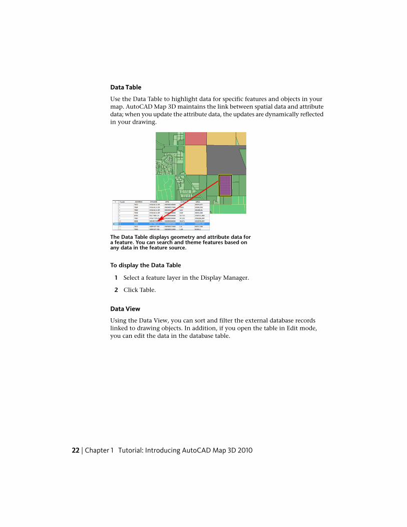
Data Table
Use the Data Table to highlight data for specific features and objects in yourmap. AutoCAD Map 3D maintains the link between spatial data and attributedata; when you update the attribute data, the updates are dynamically reflectedin your drawing.
The Data Table displays geometry and attribute data fora feature. You can search and theme features based onany data in the feature source.
To display the Data Table
1 Select a feature layer in the Display Manager.
2 Click Table.
Data View
Using the Data View, you can sort and filter the external database recordslinked to drawing objects. In addition, if you open the table in Edit mode,you can edit the data in the database table.
22 | Chapter 1 Tutorial: Introducing AutoCAD Map 3D 2010
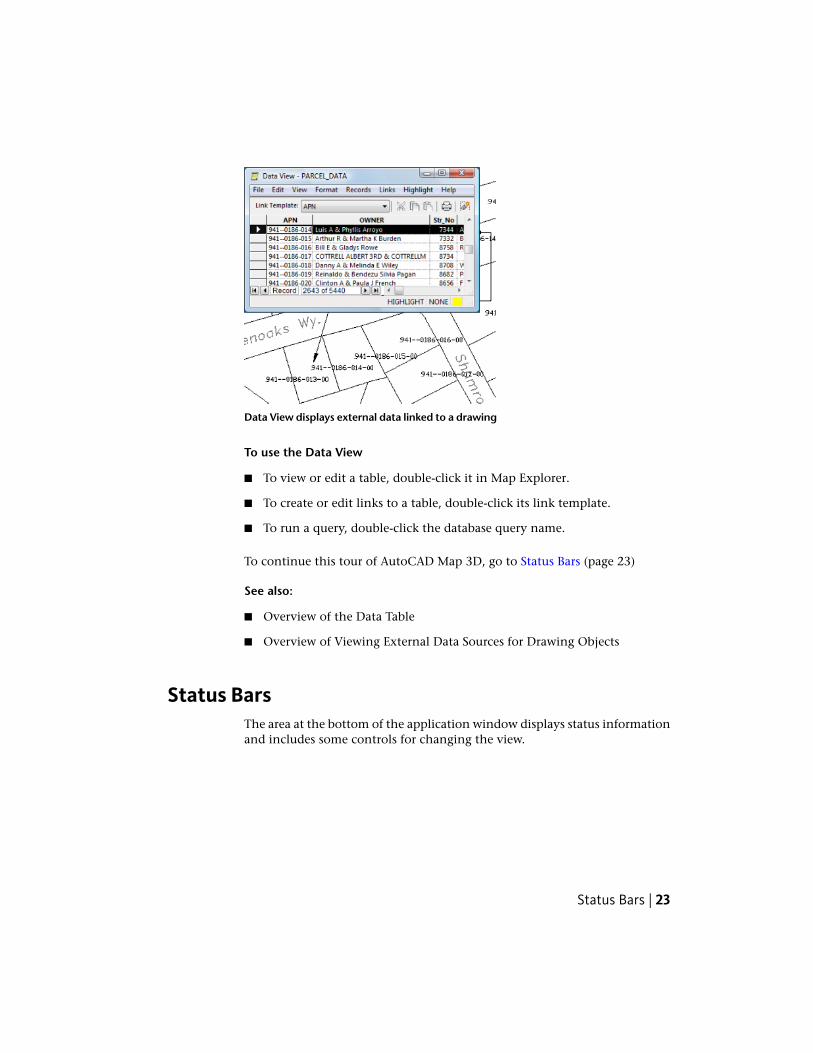
Data View displays external data linked to a drawing
To use the Data View
■ To view or edit a table, double-click it in Map Explorer.
■ To create or edit links to a table, double-click its link template.
■ To run a query, double-click the database query name.
To continue this tour of AutoCAD Map 3D, go to Status Bars (page 23)
See also:
■ Overview of the Data Table
■ Overview of Viewing External Data Sources for Drawing Objects
Status BarsThe area at the bottom of the application window displays status informationand includes some controls for changing the view.
Status Bars | 23
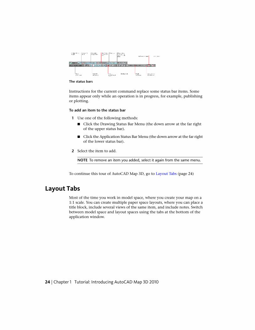
The status bars
Instructions for the current command replace some status bar items. Someitems appear only while an operation is in progress, for example, publishingor plotting.
To add an item to the status bar
1 Use one of the following methods:
■ Click the Drawing Status Bar Menu (the down arrow at the far rightof the upper status bar).
■ Click the Application Status Bar Menu (the down arrow at the far rightof the lower status bar).
2 Select the item to add.
NOTE To remove an item you added, select it again from the same menu.
To continue this tour of AutoCAD Map 3D, go to Layout Tabs (page 24)
Layout TabsMost of the time you work in model space, where you create your map on a1:1 scale. You can create multiple paper space layouts, where you can place atitle block, include several views of the same item, and include notes. Switchbetween model space and layout spaces using the tabs at the bottom of theapplication window.
24 | Chapter 1 Tutorial: Introducing AutoCAD Map 3D 2010
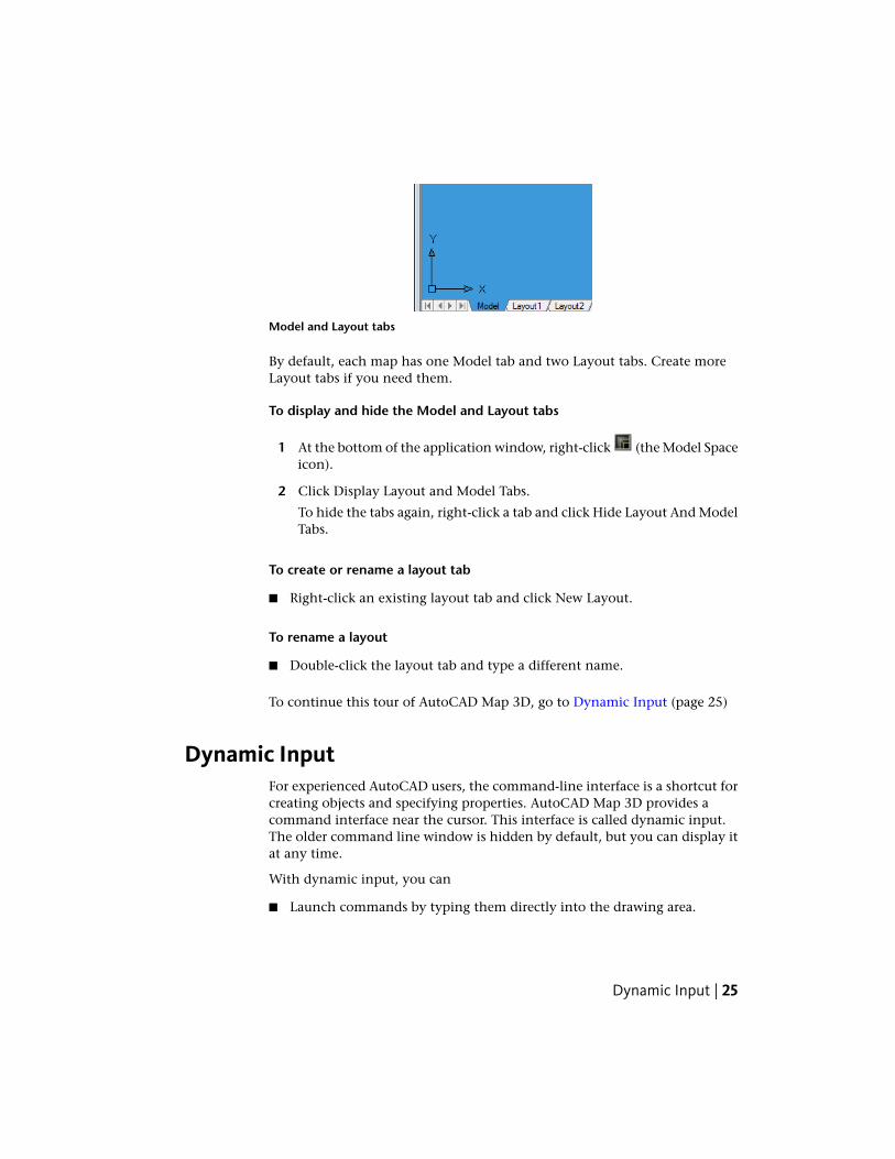
Model and Layout tabs
By default, each map has one Model tab and two Layout tabs. Create moreLayout tabs if you need them.
To display and hide the Model and Layout tabs
1 At the bottom of the application window, right-click (the Model Spaceicon).
2 Click Display Layout and Model Tabs.
To hide the tabs again, right-click a tab and click Hide Layout And ModelTabs.
To create or rename a layout tab
■ Right-click an existing layout tab and click New Layout.
To rename a layout
■ Double-click the layout tab and type a different name.
To continue this tour of AutoCAD Map 3D, go to Dynamic Input (page 25)
Dynamic InputFor experienced AutoCAD users, the command-line interface is a shortcut forcreating objects and specifying properties. AutoCAD Map 3D provides acommand interface near the cursor. This interface is called dynamic input.The older command line window is hidden by default, but you can display itat any time.
With dynamic input, you can
■ Launch commands by typing them directly into the drawing area.
Dynamic Input | 25

■ Respond to command prompts in a tooltip or tooltip menu near the cursor,instead of on the command line.
■ View the location of the crosshairs as coordinate values in a tooltip.
■ Enter coordinate values in the tooltip when a command prompts for apoint, instead of on the command line.
■ View distance and angle values when a command prompts for a secondpoint.
An example of dynamic input
NOTE With the command line hidden, detailed information for some commandsis not visible. To see this information, display the command line by pressing CTRL+9on the keyboard.
Keep in mind the following rules :
■ Some commands require that you specify vectors with your cursor. Whenyou finish, press Esc.
■ Some commands require that you select an object. Click the object andpress Enter.
■ Some commands have multiple input fields. Press the Tab key to movefrom one to another.
26 | Chapter 1 Tutorial: Introducing AutoCAD Map 3D 2010

■ When the down arrow icon appears in a prompt, press the down arrowon your keyboard to see a list of options for that command. Press the downarrow again to move between options, and then press Enter to select thehighlighted one.
To use dynamic input
1 Position your cursor over an empty space in the map.
2 Enter circle and press Enter.
3 Respond to the prompts to draw a circle.
■ For the center point of the circle, click somewhere in the map.
■ For the radius of the circle, enter 500 and press Enter.
To turn dynamic input on or off
■ On the status bar, click , or press F12.
To turn off dynamic input temporarily
■ Hold down the F12 key while you work.
To control dynamic input settings
■ Right-click and click Settings.
NOTE By default, dynamic input is set to relative (not absolute) coordinates.For example, entering 10,10 and then 20,20 draws a line from 10,10 to 30,30.If you frequently enter absolute coordinates, you can change this setting.
To hide or show the command line window
■ Press CTRL+9 on the keyboardTo display the AutoCAD text window with all your past command-lineinput history, press F2. To hide this information, press F2 again.
To continue this tour of AutoCAD Map 3D, go to Shortcut Menus (page 28)
Dynamic Input | 27
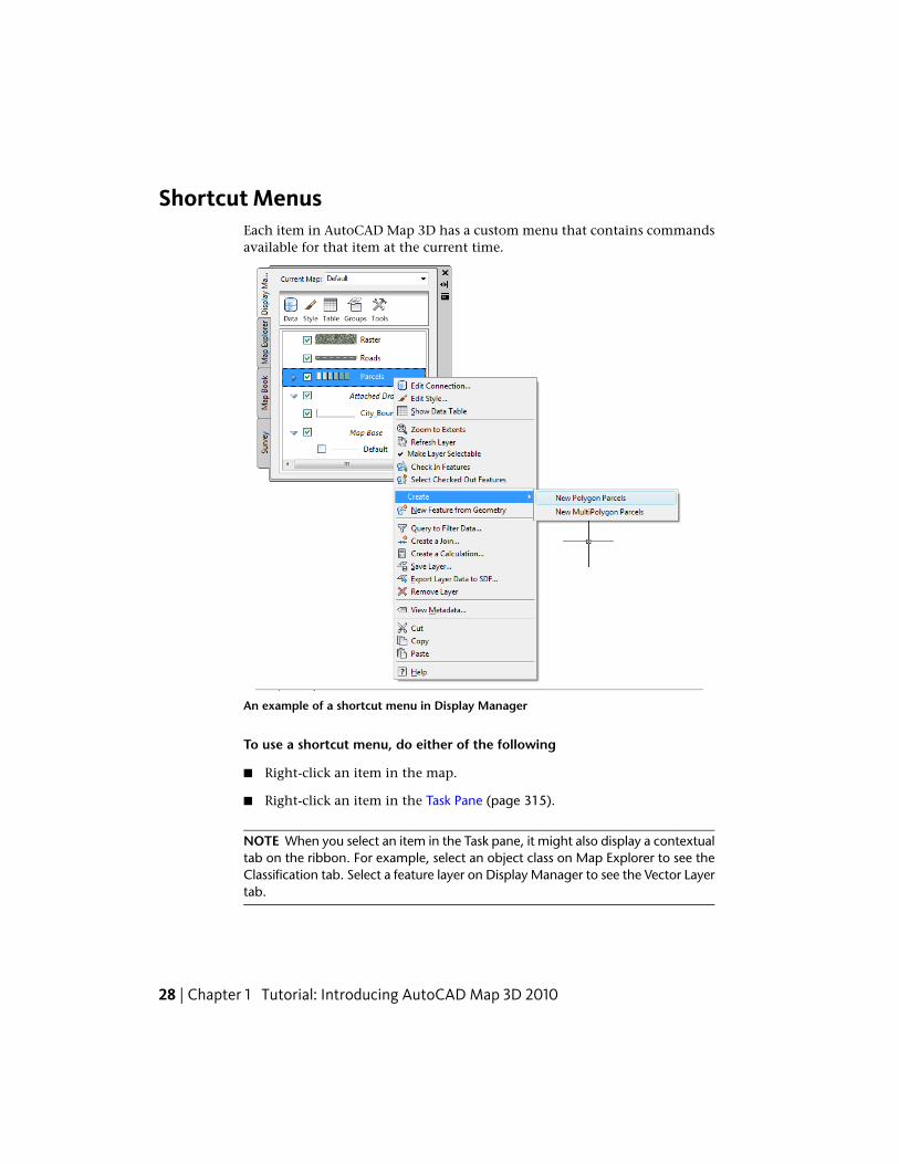
Shortcut MenusEach item in AutoCAD Map 3D has a custom menu that contains commandsavailable for that item at the current time.
An example of a shortcut menu in Display Manager
To use a shortcut menu, do either of the following
■ Right-click an item in the map.
■ Right-click an item in the Task Pane (page 315).
NOTE When you select an item in the Task pane, it might also display a contextualtab on the ribbon. For example, select an object class on Map Explorer to see theClassification tab. Select a feature layer on Display Manager to see the Vector Layertab.
28 | Chapter 1 Tutorial: Introducing AutoCAD Map 3D 2010
To continue this tour of AutoCAD Map 3D, go to Options (page 29)
OptionsYou can set two sets of options in AutoCAD Map 3D: AutoCAD options andAutoCAD Map 3D options.
AutoCAD options affect your map in some ways. For example, you can changethe background color for maps using these options.
AutoCAD Map 3D options are all specific to mapping.
To change AutoCAD options
1 Click to see the application menu.
The application menu remains displayed until you select a command orclick somewhere else.
2 Click Options (at the bottom of the menu).
3 Change any options you like. For example, to change the backgroundcolor of all future maps, change the following option:
■ Click the Display tab.
■ Click Colors.Under Context, 2D Model Space should be selected. Under InterfaceElement, Uniform Background should be selected.
■ Change the value for Color.Select any color.
■ Click Apply & Close.
To change AutoCAD Map 3D options
1 Click Map Setup tab ➤ Map panel ➤ angle-arrow.
2 Click a tab.
3 Modify options.
4 Click OK to save the settings.
Options | 29
See also:
■ Overview of Setting Options
Lesson 3: Get StartedThis lesson provides an overview of the basic tasks needed for creating maps.
In this lesson, you use the Display Manager. Bring in a file containing roaddata, change the way the roads are displayed, and then save your work. Inabout 15 minutes, you will have a complete map.
Exercise 1: Create a mapCreate a map file using a standard template. Assign a coordinate system. Anydata you add to your map is converted to that coordinate system.
To create a map
1 Before you begin this tutorial, see Lesson 1: Get Ready to Use the Tutorials(page 1).
2 From your desktop or the Start menu, start AutoCAD Map 3D (if it is notalready running).
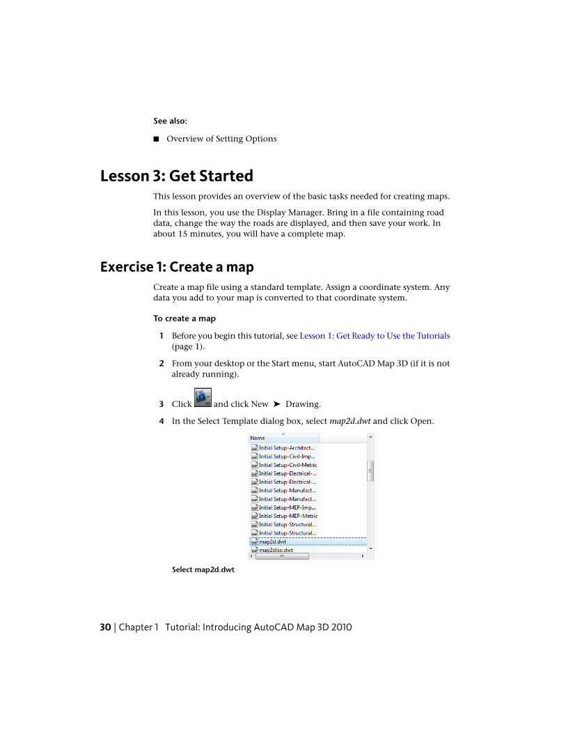
3 Click and click New ➤ Drawing.
4 In the Select Template dialog box, select map2d.dwt and click Open.
Select map2d.dwt
30 | Chapter 1 Tutorial: Introducing AutoCAD Map 3D 2010

This file is an AutoCAD template that is set up to work withtwo-dimensional maps in AutoCAD Map 3D.
5 Assign a coordinate system for your map.
■ In the Task pane, click the Map Explorer tab.
■ In Map Explorer (page 312), right-click Current Drawing and clickCoordinate System.
Set the coordinate system from the Task pane.
■ In the Assign Global Coordinate System dialog box, for Code, enterCA-I . (Enter the letters CA, hyphen, letter I.)
Specify the code for your coordinate system.
Exercise 1: Create a map | 31

NOTE To find the code for a particular coordinate system, click SelectCoordinate System in this dialog box and select a coordinate system bycategory. Use the Properties button to see information about differentcoordinate systems until you find the one for your map.
■ Click OK.
Exercise 2: Use Data Connect to add data to your mapUse Display Manager to bring in a file containing road data.
To add data to your map
1 In the Task Pane (page 315), switch to Display Manager (page 310).
2 In the Display Manager menu area, click Data ➤ Connect To Data.
Use the Data menu in the Task pane toadd any type of data to a map.
The Data Connect (page 310) window is displayed.
3 Under Data Connections By Provider (on the left side), click Add SHPConnection.
4 Click the file icon next to Source File Or Folder (on the right side).
5 Navigate to the sample data folder (page 2) and select Roads.shp. ClickOpen.
32 | Chapter 1 Tutorial: Introducing AutoCAD Map 3D 2010

6 Click Connect to add the Roads SHP file as a data source.
To add a feature, first connect to its source.
7 In the Data Connect window, click Add to Map.
Click Add To Map to see the data in your map.
8 Close the Data Connect window by clicking the X at the top.
Exercise 3: Style a featureChange the appearance of the roads.
Exercise 3: Style a feature | 33

To style the roads
1 In Display Manager (page 310), select the layer labeled Roads and clickStyle in the menu area.
Select the Roads layer and click Style.
The Style Editor window is displayed over your map.
2 In the Style Editor window, click for Style and select a thickness, color,and pattern for the roads. Click OK.
34 | Chapter 1 Tutorial: Introducing AutoCAD Map 3D 2010
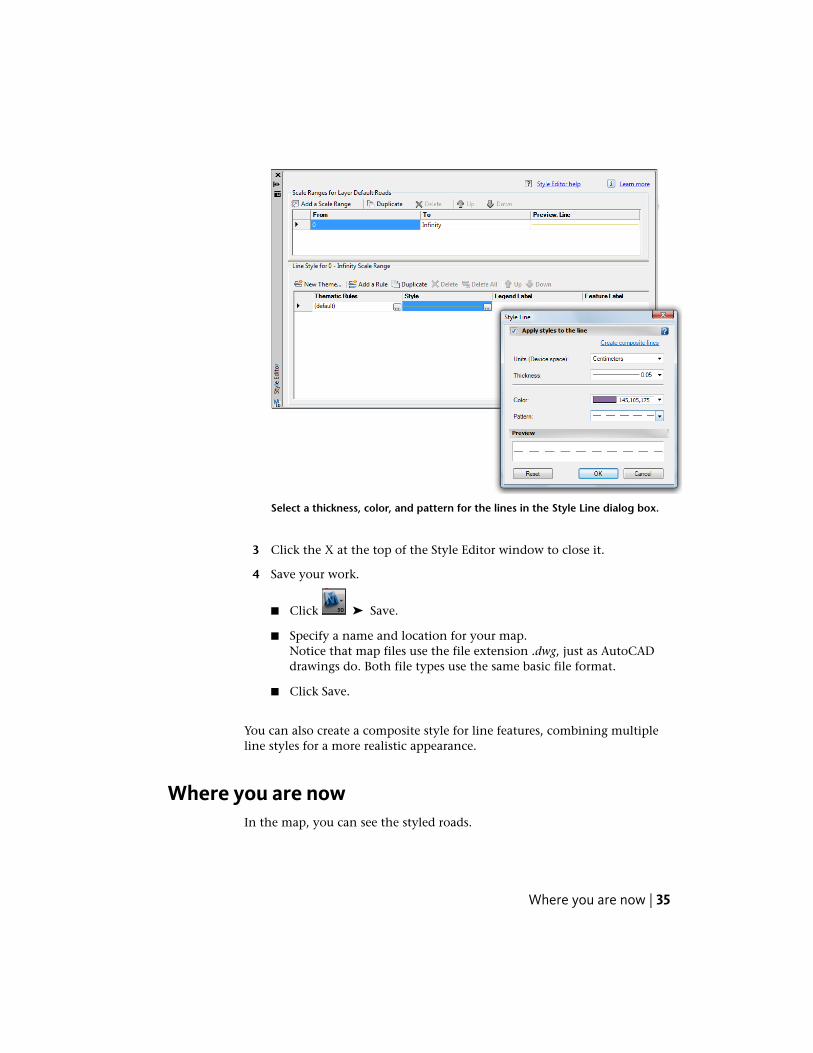
Select a thickness, color, and pattern for the lines in the Style Line dialog box.
3 Click the X at the top of the Style Editor window to close it.
4 Save your work.
■ Click ➤ Save.
■ Specify a name and location for your map.Notice that map files use the file extension .dwg, just as AutoCADdrawings do. Both file types use the same basic file format.
■ Click Save.
You can also create a composite style for line features, combining multipleline styles for a more realistic appearance.
Where you are nowIn the map, you can see the styled roads.
Where you are now | 35

36 | Chapter 1 Tutorial: Introducing AutoCAD Map 3D 2010
Tutorial: Building a Map
About the Building a Map TutorialThe lessons in this tutorial take you through the entire workflow of buildingand publishing a map. You use real data from the city of Redding, Californiato do the following:
■ Start a map project by connecting to all the data stores needed by your map.Data stores can include geospatial databases, spatial data files, such as Shape(SHP) and SDF files, AutoCAD drawings (DWG files), and raster images.Connecting to a data store makes the information in that data store availableto your map.
■ Style the objects in your map so you can easily identify them. Styles canhelp you provide complex information quickly and intuitively. For example,themed styles can show population density, water depth, or the relativeheight of geographic features.
■ Edit objects in your map. In AutoCAD Map 3D, you can check out and editany type of object using AutoCAD commands. For example, edit geometryin a drawing file, a schema in an ESRI SHP file, or geospatial data stored inan Oracle database. You can then save the changes back into their originalformat. You can also use the Data Table to change the properties of geospatialdata.
■ Publish the resulting map for display on a web site. In this tutorial, youpublish to DWF format (for use with Autodesk Design Review). You can alsopublish or export to Autodesk MapGuide, or save your map as a static webpage.
2
37

Lesson 1: Use Multiple SourcesIn the first set of lessons, you practice connecting to data from various sources.
Exercise 1: Drag and drop a source fileStart by creating a map file and adding the city boundaries of Redding to it.
To create a map and add a source file
1 Before you begin this tutorial, see Lesson 1: Get Ready to Use the Tutorials(page 1).
2 Create a map file.
■ Click ➤ New ➤ Drawing.
■ Select the map2d.dwt template.
■ Click Open.
3 Set the coordinate system for the map.
■ Switch to Map Explorer (page 312) in the Task Pane (page 315).
■ Right-click Current Drawing and click Coordinate System.
■ Enter CA-I and click OK.
4 Add the city boundaries to your map by dragging and dropping a sourcefile to Display Manager.
■ Switch to Display Manager (page 310) in the Task pane.
■ Use Windows Explorer to navigate to the folder in My Documentswhere you copied the sample files.
NOTE The location of My Documents varies, depending on your operatingsystem. For Microsoft Windows XP, it is usually C:\MyDocuments. ForMicrosoft Vista, it might be C:\Documents and Settings\Administrator\MyDocuments\Map 3D Tutorials.
■ Resize the AutoCAD Map 3D window and your sample data folderwindow so you can see both of them at the same time.
38 | Chapter 2 Tutorial: Building a Map
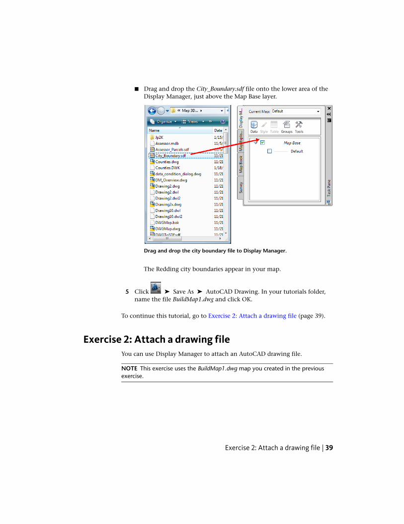
■ Drag and drop the City_Boundary.sdf file onto the lower area of theDisplay Manager, just above the Map Base layer.
Drag and drop the city boundary file to Display Manager.
The Redding city boundaries appear in your map.
5 Click ➤ Save As ➤ AutoCAD Drawing. In your tutorials folder,name the file BuildMap1.dwg and click OK.
To continue this tutorial, go to Exercise 2: Attach a drawing file (page 39).
Exercise 2: Attach a drawing fileYou can use Display Manager to attach an AutoCAD drawing file.
NOTE This exercise uses the BuildMap1.dwg map you created in the previousexercise.
Exercise 2: Attach a drawing file | 39
To attach an AutoCAD drawing file
1 If you have not already done so, copy the \Program Files\AutoCAD Map3D 2010\Help\Map 3D Tutorials folder to My Documents.
NOTE The location of My Documents varies, depending on your operatingsystem. For Microsoft Windows XP, it is usually C:\MyDocuments. For MicrosoftVista, it might be C:\Documents and Settings\Administrator\My Documents\Map3D Tutorials.
2 In the BuildMap1.dwg file, in the Task pane, click the Display Managertab.
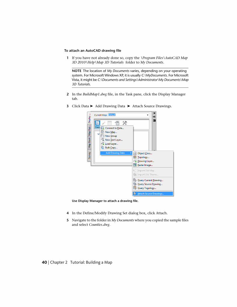
3 Click Data ➤ Add Drawing Data ➤ Attach Source Drawings.
Use Display Manager to attach a drawing file.
4 In the Define/Modify Drawing Set dialog box, click Attach.
5 Navigate to the folder in My Documents where you copied the sample filesand select Counties.dwg.
40 | Chapter 2 Tutorial: Building a Map
NOTE The location of My Documents varies, depending on your operatingsystem. For Microsoft Windows XP, it is usually C:\MyDocuments. For MicrosoftVista, it might be C:\Documents and Settings\Administrator\My Documents\Map3D Tutorials.
6 Click Add and then click OK.
7 In the Define/Modify Drawing Set dialog box, click OK to attach thedrawing file to your map.
When you attach a drawing, it is not listed in Display Manager (page 310)and it does not appear in your map. You “query in” objects from thedrawing to use in your map, as demonstrated in the next exercise.
8 Save your work. Click ➤ Save As ➤ AutoCAD Drawing.
To continue this tutorial, go to Exercise 3: Query in data from the drawing(page 41).
Exercise 3: Query in data from the drawingWhen you attach a drawing to a map, objects in the drawing do not appearin the map immediately. You must query them in. The drawing file youattached is a map of California with polygons defined for each county. Sincethe city of Redding is in Shasta County, you add the Shasta County boundariesto your map. You can query in data based on location, properties, or data. Inthis case, query the name of the county, which is stored as object data.
NOTE This exercise uses the BuildMap1.dwg map you created and modified in theprevious exercises.
To query in drawing data
1 In the BuildMap1.dwg file, in Display Manager (page 310), click Data ➤
Add Drawing Data ➤ Query Source Drawing.
2 In the Define Query Of Attached Drawings dialog box, under Query Type,click Data.
3 In the Data Condition dialog box, select the Object Data option.
4 In the Object Data Fields list, select NAME.
Exercise 3: Query in data from the drawing | 41
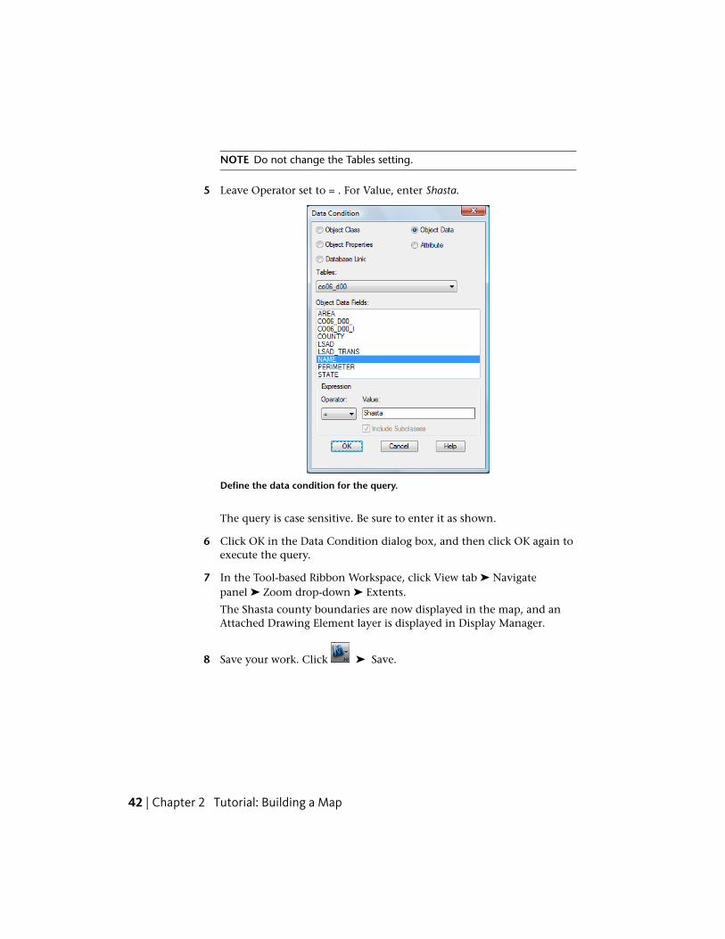
NOTE Do not change the Tables setting.
5 Leave Operator set to = . For Value, enter Shasta.
Define the data condition for the query.
The query is case sensitive. Be sure to enter it as shown.
6 Click OK in the Data Condition dialog box, and then click OK again toexecute the query.
7 In the Tool-based Ribbon Workspace, click View tab ➤ Navigatepanel ➤ Zoom drop-down ➤ Extents.
The Shasta county boundaries are now displayed in the map, and anAttached Drawing Element layer is displayed in Display Manager.
8 Save your work. Click ➤ Save.
42 | Chapter 2 Tutorial: Building a Map

NOTE You might see an alert as you work through the remainder of the tutorial.It warns that the association between queried objects in the current and attacheddrawings is not retained once the current drawing file is closed. This messagereminds you to save back any changes you make to the original drawing file. Sinceyou do not edit the Shasta County drawing in this tutorial, you can safely ignorethe alert.
To continue this tutorial, go to Exercise 4: Use Data Connect (page 43).
Exercise 4: Use Data ConnectUse Data Connect (page 310) to connect your map to a file containing parceldata.
Use the Data Connect window to attach any non-DWG data source:
■ Database formats, such as ArcSDE, Oracle, or SQL Server
■ An ODBC source, such as Microsoft Access
■ A raster file
■ Web-based sources such as WMS or WFS
■ Spatial data files, such as SDF and SHP
Data Connect displays information about all attached non-DWG data sources,even if you did not use Data Connect to attach them. For example, the SDFfile you dragged and dropped into your map is listed in the Data Connectwindow.
NOTE This exercise uses the BuildMap1.dwg map you created and modified in theprevious exercises.
To use Data Connect
1 If you have not already done so, copy the \Program Files\AutoCAD Map3D 2010\Help\Map 3D Tutorials folder to My Documents.
NOTE The location of My Documents varies, depending on your operatingsystem. For Microsoft Windows XP, it is usually C:\MyDocuments. For MicrosoftVista, it might be C:\Documents and Settings\Administrator\My Documents\Map3D Tutorials.
Exercise 4: Use Data Connect | 43
2 In the BuildMap1.dwg file, in Display Manager (page 310), click Data ➤
Connect to Data.
3 Under Data Connections By Provider, select Add SDF Connection.
4 Click the file icon next to Source File.
5 Navigate to the folder in My Documents where you copied the sample filesand select PARCELS.SDF. Click Open.
6 Click Connect to add the parcel data file as a data source.
Under Add Data To Map, Parcels is selected.
The coordinate system for this feature class is displayed next to its name.If this information was incorrect, you could click the current coordinatesystem listing to see a down arrow and select a different coordinate system.
NOTE Change the incoming coordinate system only if you know the originalcoordinate system for the feature—do not change the coordinate system tomatch your map. AutoCAD Map 3D automatically converts each feature fromits own coordinate system into the coordinate system for the current map.If you change the coordinate system, the conversion might not be correct.
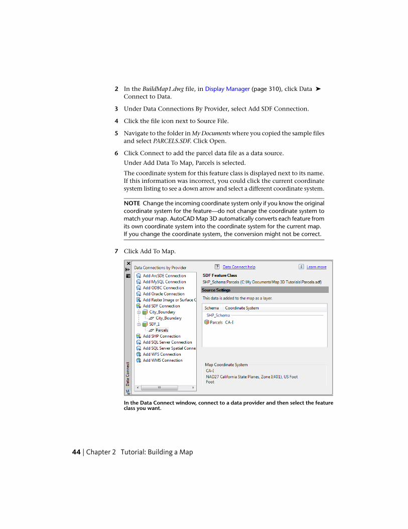
7 Click Add To Map.
In the Data Connect window, connect to a data provider and then select the featureclass you want.
44 | Chapter 2 Tutorial: Building a Map
When you click Add To Map, a layer called Parcels is displayed in the listin the Display Manager (page 310). A layer can be styled, saved, displayed,or hidden, independent of other layers in your map.
8 Save your work. Click ➤ Save.
To continue this tutorial, go to Exercise 5: Add a raster image (page 45).
Exercise 5: Add a raster imagePhotographs and other images formed of pixels are called raster images, whileimages formed of lines and arcs are called vector images. Bring in an aerialphotograph to display behind the objects in your map. Real-world elementsin the raster image line up with the geometry in your map and make it easierfor the viewer to get a visual orientation.
NOTE This exercise uses the BuildMap1.dwg map you created and modified in theprevious exercises.
To add a raster image
1 If you have not already done so, copy the \Program Files\AutoCAD Map3D 2010\Help\Map 3D Tutorials folder to My Documents.
NOTE The location of My Documents varies, depending on your operatingsystem. For Microsoft Windows XP, it is usually C:\MyDocuments. For MicrosoftVista, it might be C:\Documents and Settings\Administrator\My Documents\Map3D Tutorials.
2 In the BuildMap1.dwg file, the Data Connect (page 310) window shouldstill be displayed. If it is not, open Display Manager (page 310). Click Data ➤ Connect To Data.
3 Under Data Connections By Provider, select Add Raster Image Or SurfaceConnection.
4 Click the folder button next to Source File Or Folder.
5 Navigate to the folder in My Documents where you copied the samplefiles. Find the folder containing the JPEG 2000 raster files (originallycalled JP2K), and select it. Click OK.
6 Click Connect to add the folder as a data source.
Exercise 5: Add a raster image | 45

7 Under Add Data To Map, select the j-05, j-07, l-05, and l-07 items.
The folder contains multiple JPEG 2000 files, each of which covers a smallarea of the city of Redding. Since there are multiple items and you mightnot want all of them, they are not selected automatically.
If your folder contains multiple images, select the ones you want.
8 Set the coordinate systems for the images.
■ Click Edit Coordinate Systems.
■ In the Global Coordinate System dialog box, click in the blank fieldin the row labeled “Default” and click Edit.
■ For Category, select USA, California.
■ Under Coordinate Systems In Category, click CA-I.
■ Click OK in both dialog boxes, to return to the Data Connect window.All the images now show CA-I as their coordinate systems.
46 | Chapter 2 Tutorial: Building a Map
9 Select Combine Into One Layer, so you can style the raster images as asingle item in Display Manager.
10 Enter a name for the layer, for example, ReddingRasterImages.
11 Click Add To Map.
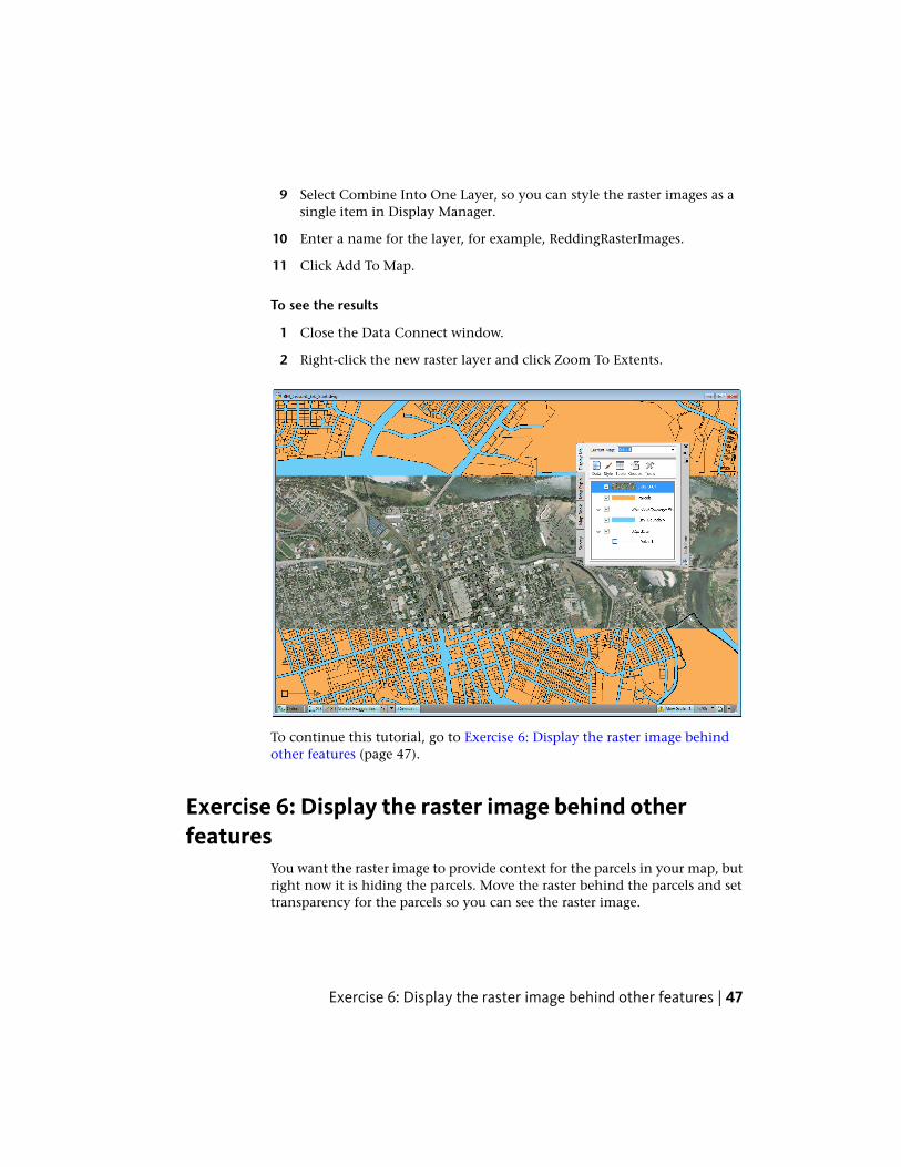
To see the results
1 Close the Data Connect window.
2 Right-click the new raster layer and click Zoom To Extents.
To continue this tutorial, go to Exercise 6: Display the raster image behindother features (page 47).
Exercise 6: Display the raster image behind otherfeatures
You want the raster image to provide context for the parcels in your map, butright now it is hiding the parcels. Move the raster behind the parcels and settransparency for the parcels so you can see the raster image.
Exercise 6: Display the raster image behind other features | 47

NOTE This exercise uses the BuildMap1.dwg map you created and modified in theprevious exercises.
To display the raster image behind other features
1 In the BuildMap1.dwg file, in the Display Manager (page 310) menu bar,make sure the fourth item reads Draw Order. If it reads Groups, click itand change it to Draw Order.
2 Drag the new raster layer just below the Parcels layer.
The list of layers is the draw order for your map. The item at the top ofthe list is also at the top of the draw order. Dragging the raster imagebelow the Parcels layer places it behind that layer in your map.
To see the raster layer behind the parcels, make the city boundary layerwhite and make the parcels semi-transparent.
3 In Display Manager, select the City_Boundary layer.
4 Click Style to see the Style Editor.
NOTE If the Style Editor is docked, move your cursor over it to display it. Itmight be docked at the left side of the application window.
5 In the Style Editor, in the Polygon Style For 0 - Infinity: Scale Rangesection, click the Style entry.
6 Change the Foreground Color to white and click OK.
7 Without closing the Style Editor, select the Parcels layer in DisplayManager.
The Data Connect window updates to show the values for the Parcelslayer.
8 In the Style Editor, click the Style entry again.
9 Move the Foreground Transparency slider to 50% and click OK.
Close the Style Editor. Right-click the Parcels layer and click Zoom ToExtents to see the results.
10 Save your map.
48 | Chapter 2 Tutorial: Building a Map

Where you are now
You have assembled all the raw materials for your map. The aerial photographprovides context. The geometry from the DWG drawing shows the countyboundaries, and the SDF files add the city boundary and parcel outlines.
To continue this tutorial, go to Lesson 2: Style Map Features (page 49)
Lesson 2: Style Map FeaturesIn the Lesson 3: Get Started (page 30) lesson, you changed the style for theroads in your map. You changed the color, thickness, and pattern for the linesrepresenting roads.
In this lesson, you use themed styles to give the viewer an immediate senseof the value of each parcel.
Exercise 1: Create a theme for the parcels layerA theme uses a range of colors to represent an analogous range of values. Youcan also use theming to show relative area, population density, water depth,or height of geographic features.
NOTE This exercise uses the BuildMap1.dwg map you created and modified in theprevious exercises.
To style the parcels layer with a theme
1 Open your finished map from the previous lesson.
■ Click ➤ Open ➤ Drawing.
■ Locate BuildMap1.dwg.
■ Select it, and click Open.
2 Create a theme for the parcel layer.
A theme is a display style. You assign styles for geospatial features bylayer.
■ In Display Manager (page 310), select the Parcels layer and click Style.
Lesson 2: Style Map Features | 49
NOTE If the Style Editor is docked, move your cursor over it to display it.It might be docked at the left side of the application window.
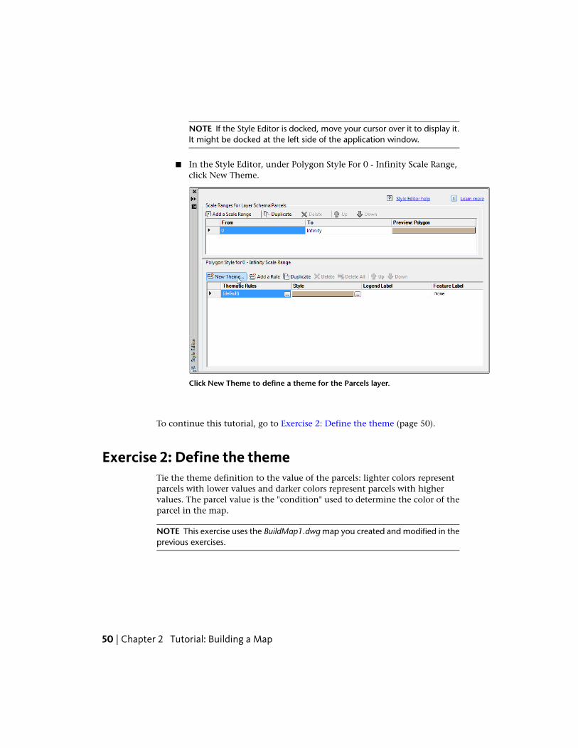
■ In the Style Editor, under Polygon Style For 0 - Infinity Scale Range,click New Theme.
Click New Theme to define a theme for the Parcels layer.
To continue this tutorial, go to Exercise 2: Define the theme (page 50).
Exercise 2: Define the themeTie the theme definition to the value of the parcels: lighter colors representparcels with lower values and darker colors represent parcels with highervalues. The parcel value is the "condition" used to determine the color of theparcel in the map.
NOTE This exercise uses the BuildMap1.dwg map you created and modified in theprevious exercises.
50 | Chapter 2 Tutorial: Building a Map

To define the theme
1 In the Theme Polygons dialog box, under Create Thematic Rules BasedOn A Property, click the down arrow next to Property and selectLAND_VALUE. Leave the minimum value, maximum value, anddistribution settings as they are.
Use the Theme Polygons dialog box to design your theme.
2 Under Theme The Polygons, click next to the illustration of the StyleRange.
3 Set Foreground transparency to 50% so you can continue to see the rasterimage below the parcels.
4 For Foreground Color Range, select colors from the color boxes underFrom and To.
5 Experiment with line thickness and color, if you like.
Exercise 2: Define the theme | 51

Set transparency, colors, and line attributes for the theme.
6 Click OK twice to return to the Style Editor. Leave the Style Editor openfor the next exercise.
To continue this tutorial, go to Exercise 3: Add labels (page 52).
Exercise 3: Add labelsAdd a label for each parcel, based on its land value.
NOTE This exercise uses the BuildMap1.dwg map you created and modified in theprevious exercises.
52 | Chapter 2 Tutorial: Building a Map
To add labels
1 In the Style Editor, click the first field in the Feature Label column.
The field value is “None.”
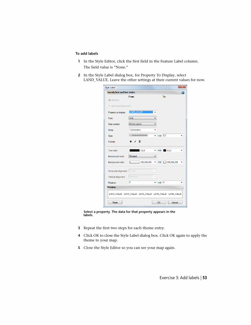
2 In the Style Label dialog box, for Property To Display, selectLAND_VALUE. Leave the other settings at their current values for now.
Select a property. The data for that property appears in thelabels.
3 Repeat the first two steps for each theme entry.
4 Click OK to close the Style Label dialog box. Click OK again to apply thetheme to your map.
5 Close the Style Editor so you can see your map again.
Exercise 3: Add labels | 53

6 Zoom in so you can see the labels. In the Tool-based Ribbon Workspace,click View tab ➤ Navigate panel ➤ Zoom Drop-down ➤ Window.
TIP The smaller you draw the zoom window, the larger the magnification.
7 Save your map.
Where you are now
In the map, the parcels are colored to represent their relative values, whichare displayed as labels on each parcel.
Themed parcels with labels
To continue this tutorial, go to Lesson 3: Change the Display by Zoom Level(page 54)
Lesson 3: Change the Display by Zoom LevelUse styles to make objects display differently, depending on the zoom level.In this example, when the viewer is zoomed in, roads are dark gray with adashed yellow centerline. When the viewer zooms out, the roads display as
54 | Chapter 2 Tutorial: Building a Map
solid black. When the viewer zooms out far enough, roads are not displayedat all.
Exercise 1: Add roads to your mapAdd roads to your map and assign several styles to them, with each styledisplaying at a different zoom level.
NOTE This exercise uses the BuildMap1.dwg map you created and modified in theprevious exercises.
To add roads to your map
1 If you have not already done so, copy the \Program Files\AutoCAD Map3D 2010\Help\Map 3D Tutorials folder to My Documents.
NOTE The location of My Documents varies, depending on your operatingsystem. For Microsoft Windows XP, it is usually C:\MyDocuments. For MicrosoftVista, it might be C:\Documents and Settings\Administrator\My Documents\Map3D Tutorials.
2 Open your finished map from the previous lesson.
■ Click ➤ Open ➤ Drawing.
■ Locate BuildMap1.dwg.
■ Select the map, and click Open.
3 In the Task Pane (page 315), switch to Display Manager (page 310) .
4 In the menu area, click Group and select Layers By Group.
5 Use Windows Explorer to navigate to the folder in My Documents whereyou copied the sample files.
6 Resize the AutoCAD Map 3D window and the sample data folder windowso you can see both of them at the same time.
7 Drag and drop the Roads.shp file to the list of layers in the DisplayManager, just above the Parcels layer.
To continue this tutorial, go to Exercise 2: Create a composite road style (page56).
Exercise 1: Add roads to your map | 55
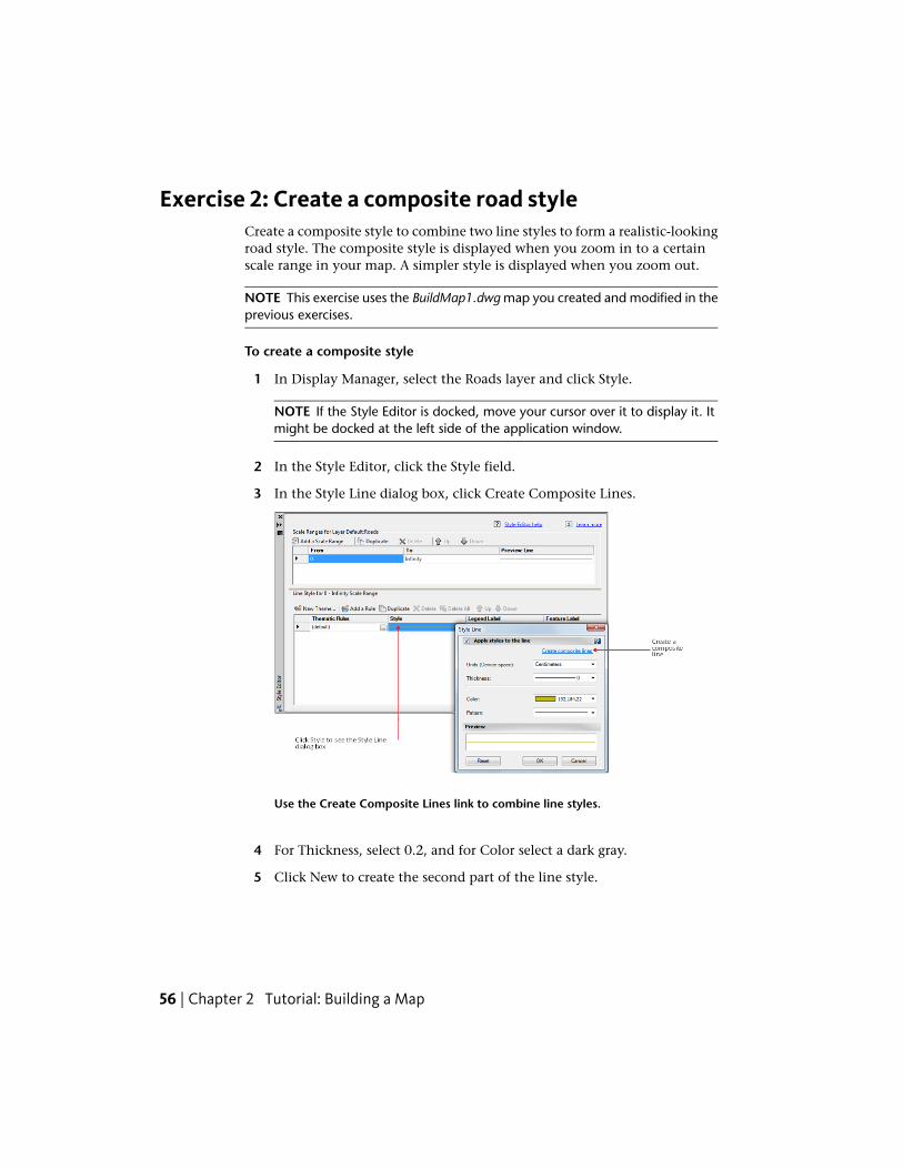
Exercise 2: Create a composite road styleCreate a composite style to combine two line styles to form a realistic-lookingroad style. The composite style is displayed when you zoom in to a certainscale range in your map. A simpler style is displayed when you zoom out.
NOTE This exercise uses the BuildMap1.dwg map you created and modified in theprevious exercises.
To create a composite style
1 In Display Manager, select the Roads layer and click Style.
NOTE If the Style Editor is docked, move your cursor over it to display it. Itmight be docked at the left side of the application window.
2 In the Style Editor, click the Style field.
3 In the Style Line dialog box, click Create Composite Lines.
Use the Create Composite Lines link to combine line styles.
4 For Thickness, select 0.2, and for Color select a dark gray.
5 Click New to create the second part of the line style.
56 | Chapter 2 Tutorial: Building a Map
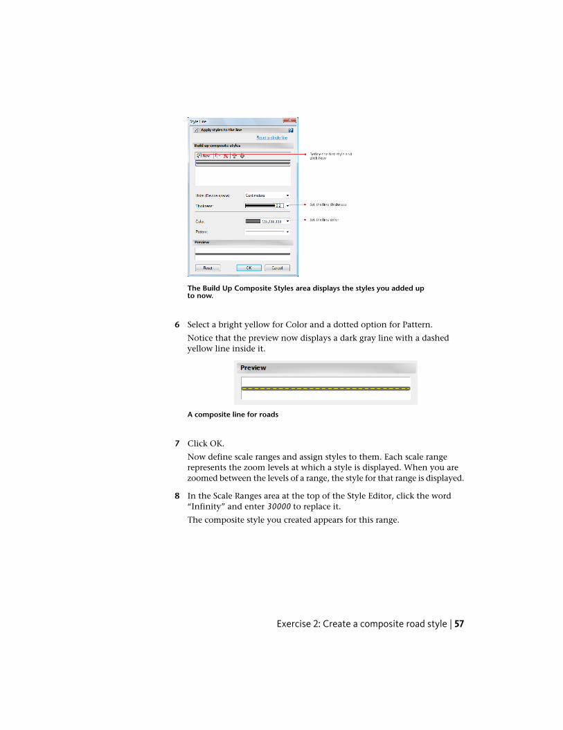
The Build Up Composite Styles area displays the styles you added upto now.
6 Select a bright yellow for Color and a dotted option for Pattern.
Notice that the preview now displays a dark gray line with a dashedyellow line inside it.
A composite line for roads
7 Click OK.
Now define scale ranges and assign styles to them. Each scale rangerepresents the zoom levels at which a style is displayed. When you arezoomed between the levels of a range, the style for that range is displayed.
8 In the Scale Ranges area at the top of the Style Editor, click the word“Infinity” and enter 30000 to replace it.
The composite style you created appears for this range.
Exercise 2: Create a composite road style | 57
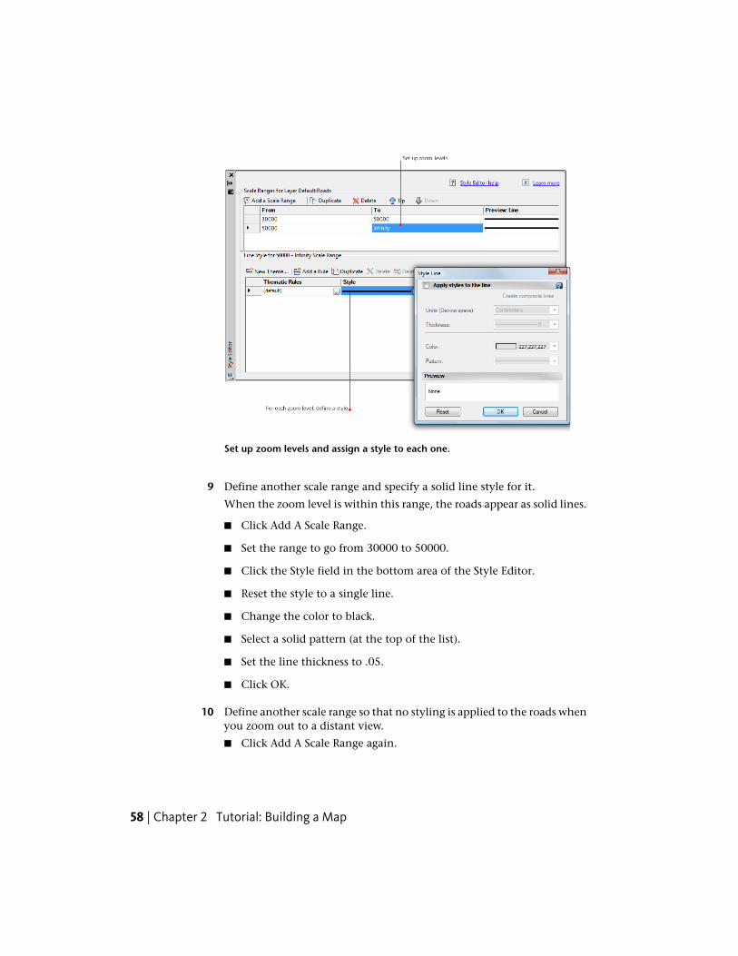
Set up zoom levels and assign a style to each one.
9 Define another scale range and specify a solid line style for it.
When the zoom level is within this range, the roads appear as solid lines.
■ Click Add A Scale Range.
■ Set the range to go from 30000 to 50000.
■ Click the Style field in the bottom area of the Style Editor.
■ Reset the style to a single line.
■ Change the color to black.
■ Select a solid pattern (at the top of the list).
■ Set the line thickness to .05.
■ Click OK.
10 Define another scale range so that no styling is applied to the roads whenyou zoom out to a distant view.
■ Click Add A Scale Range again.
58 | Chapter 2 Tutorial: Building a Map
■ Set the new range to go from 50000 to infinity.
■ Click the Style field in the bottom area of the Style Editor.
■ Clear the Apply Styles To The Line check box at the top of the StyleLine dialog box.
■ Click OK.
The style for this scale range is now None. When you zoom out to adistant view, you cannot see the roads.
11 Close the Style Editor.
12 Save the file.
To continue this tutorial, go to Exercise 3: View styles at different zoom levels(page 59).
Exercise 3: View styles at different zoom levelsZoom to different scales in your map to see the different line styles.
NOTE This exercise uses the BuildMap1.dwg map you created and modified in theprevious exercises.
To see the styles at different zoom levels
1 In the BuildMap1.dwg file, use the Zoom Window tool to zoom in so youcan see the labels and the composite lines. In the Tool-based RibbonWorkspace, click View tab ➤ Navigate panel ➤ Zoomdrop-down ➤ Window.
TIP The smaller you draw the zoom window, the larger the magnification.
2 Zoom out to see thinner black lines for the roads.
3 Zoom out even farther until the roads are not displayed.
4 Save your map.
Where you are now
In the map, the roads are themed to display appropriately at different zoomlevels.
Exercise 3: View styles at different zoom levels | 59

At a scale of 1:10000, the roads display the composite style.
To continue this tutorial, go to Lesson 4: Create Map Features (page 60)
Lesson 4: Create Map FeaturesUse the powerful editing abilities of AutoCAD to draw new features.
Exercise 1: Draw a new parcelWhen you draw a new feature, it is automatically added to the layer fromwhich it was created. The source for that layer is updated to include the featureyou added.
NOTE This exercise uses the BuildMap1.dwg map you created and modified in theprevious exercises.
To create a feature
1 If it is not still open, open your map from the previous lesson.
■ Click ➤ Open ➤ Drawing.
■ Locate the BuildMap1.dwg file.
60 | Chapter 2 Tutorial: Building a Map
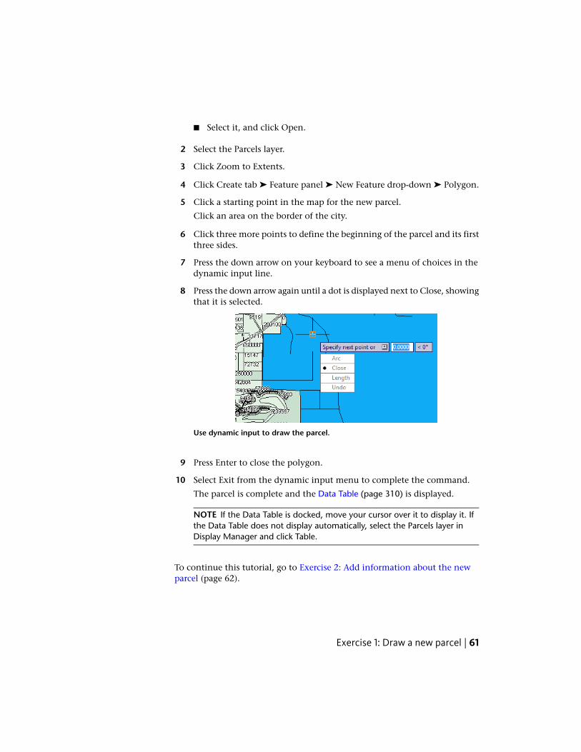
■ Select it, and click Open.
2 Select the Parcels layer.
3 Click Zoom to Extents.
4 Click Create tab ➤ Feature panel ➤ New Feature drop-down ➤ Polygon.
5 Click a starting point in the map for the new parcel.
Click an area on the border of the city.
6 Click three more points to define the beginning of the parcel and its firstthree sides.
7 Press the down arrow on your keyboard to see a menu of choices in thedynamic input line.
8 Press the down arrow again until a dot is displayed next to Close, showingthat it is selected.
Use dynamic input to draw the parcel.
9 Press Enter to close the polygon.
10 Select Exit from the dynamic input menu to complete the command.
The parcel is complete and the Data Table (page 310) is displayed.
NOTE If the Data Table is docked, move your cursor over it to display it. Ifthe Data Table does not display automatically, select the Parcels layer inDisplay Manager and click Table.
To continue this tutorial, go to Exercise 2: Add information about the newparcel (page 62).
Exercise 1: Draw a new parcel | 61
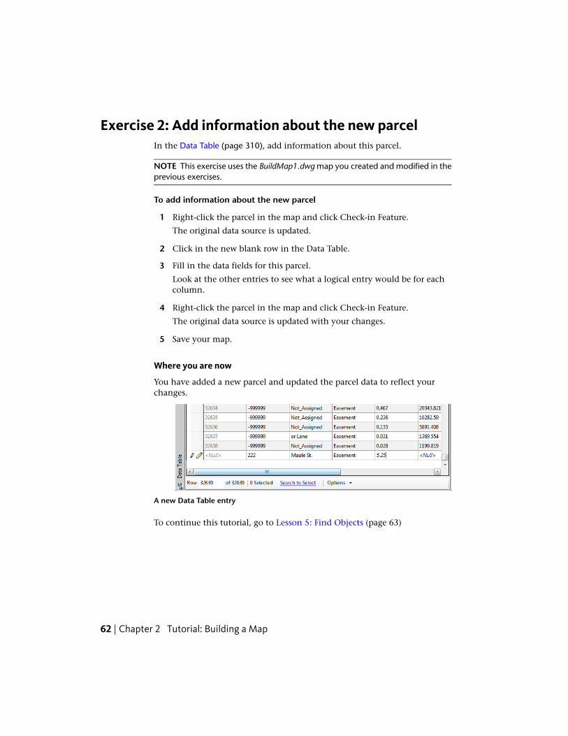
Exercise 2: Add information about the new parcelIn the Data Table (page 310), add information about this parcel.
NOTE This exercise uses the BuildMap1.dwg map you created and modified in theprevious exercises.
To add information about the new parcel
1 Right-click the parcel in the map and click Check-in Feature.
The original data source is updated.
2 Click in the new blank row in the Data Table.
3 Fill in the data fields for this parcel.
Look at the other entries to see what a logical entry would be for eachcolumn.
4 Right-click the parcel in the map and click Check-in Feature.
The original data source is updated with your changes.
5 Save your map.
Where you are now
You have added a new parcel and updated the parcel data to reflect yourchanges.
A new Data Table entry
To continue this tutorial, go to Lesson 5: Find Objects (page 63)
62 | Chapter 2 Tutorial: Building a Map
Lesson 5: Find ObjectsUse the Data Table (page 310) to find objects that match certain criteria. Then,use the Data Table to zoom in to that area of your map.
Exercise 1: Display the Data Table
NOTE This exercise uses the BuildMap1.dwg map you created and modified in theprevious exercises.
Display the Data Table (page 310) for any layer.
To display the Data Table
1 If it is not still open, open your finished map from Lesson 4: Create MapFeatures (page 60).
■ Click ➤ Open ➤ Drawing.
■ Locate the BuildMap1.dwg file.
■ Select it and click Open.
2 In the Task pane, switch to Display Manager (page 310).
3 In Display Manager, select the Parcels layer and click Table.
4 If the Data Table is docked against the left side of the application window,move your cursor over it to see its contents.
To continue this tutorial, go to Exercise 2: Filter the Data Table (page 63).
Exercise 2: Filter the Data TableFilter the Data Table (page 310) to show a subset of parcels—in this case, onlyparcels on Villa Drive.
NOTE This exercise uses the BuildMap1.dwg map you created and modified in theprevious exercises.
Lesson 5: Find Objects | 63
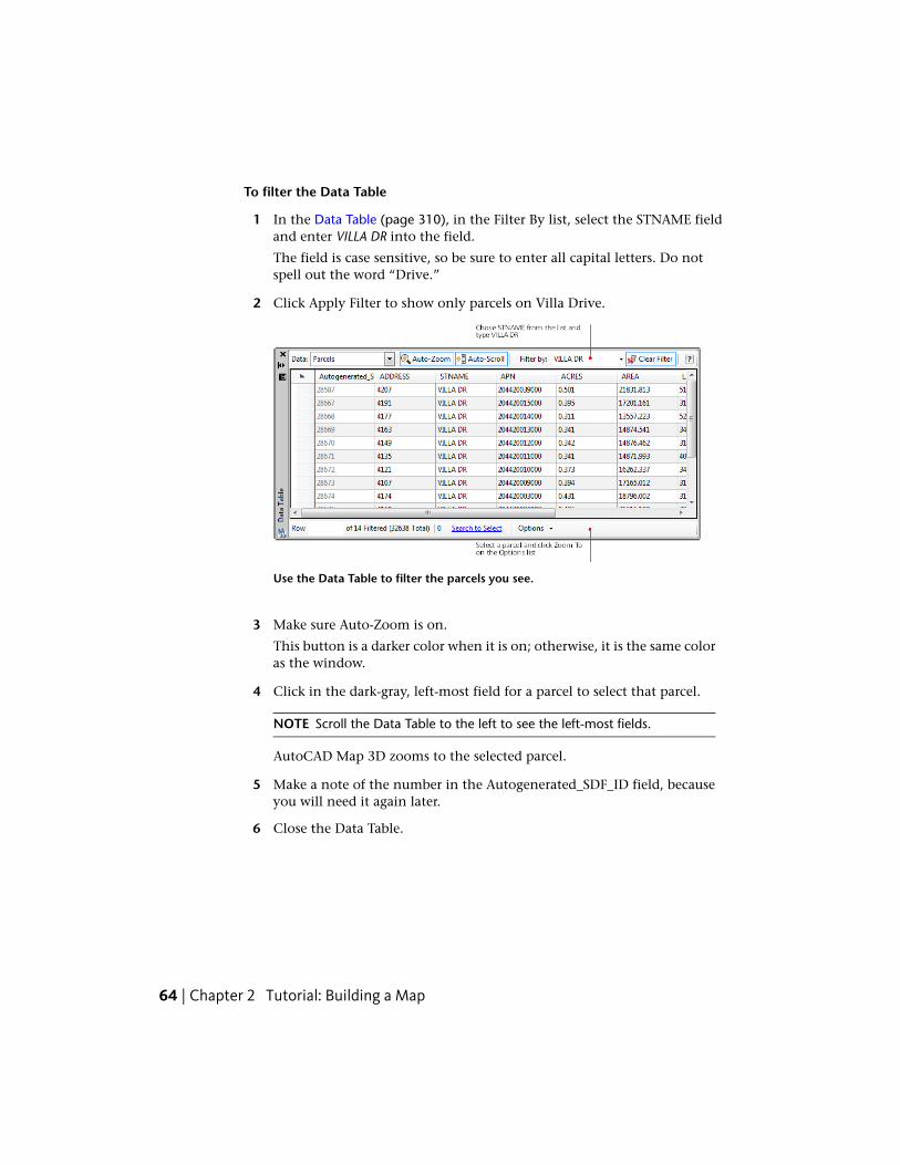
To filter the Data Table
1 In the Data Table (page 310), in the Filter By list, select the STNAME fieldand enter VILLA DR into the field.
The field is case sensitive, so be sure to enter all capital letters. Do notspell out the word “Drive.”
2 Click Apply Filter to show only parcels on Villa Drive.
Use the Data Table to filter the parcels you see.
3 Make sure Auto-Zoom is on.
This button is a darker color when it is on; otherwise, it is the same coloras the window.
4 Click in the dark-gray, left-most field for a parcel to select that parcel.
NOTE Scroll the Data Table to the left to see the left-most fields.
AutoCAD Map 3D zooms to the selected parcel.
5 Make a note of the number in the Autogenerated_SDF_ID field, becauseyou will need it again later.
6 Close the Data Table.
64 | Chapter 2 Tutorial: Building a Map
NOTE You can do a more sophisticated search. Click Home tab ➤ Data
panel ➤ Search. That option lets you query a layer with a Booleancondition—for example, ACRES > 1 to find parcels that are larger than anacre. The map then shows only the objects that match your query.
7 Save your map, but leave it open for the next lesson.
Where you are now
You used the Data Table to zoom to a parcel.
To continue this tutorial, go to Lesson 6: Edit Objects (page 65)
Lesson 6: Edit ObjectsEdit objects and then update their original data stores.
Exercise 1: Check out and edit a featureIf AutoCAD Map 3D is set to check in your changes automatically, the sourcefile updates while you edit. Automatic update can result in inadvertent changesto the data store. The safest way to edit geospatial data is to turn off automaticupdate feature before you edit a feature. Once you make your changes, checkthe feature in to update the data store with your changes and make the featureavailable to others again.
When you edit a feature, that feature is automatically checked out and lockedfor editing by anyone else (if the data format supports such locking). Otherpeople can view the feature source, but they cannot change it until you checkit back in.
NOTE This exercise uses the BuildMap1.dwg map you created and modified in theprevious exercises.
To edit an object
1 If you closed your finished map from the previous lesson, reopen it anddisplay the Data Table for the Parcels layer.
■ Click ➤ Open ➤ Drawing.
Lesson 6: Edit Objects | 65

■ Locate the BuildMap1.dwg file.
■ Select it, and click Open.
■ In the Display Manager, click the Parcels layer and click Table.
■ Zoom to a parcel on Villa Drive.
The parcel is checked outautomatically and displays grips.
2 Turn off the automatic update option. Click Feature Edit tab ➤ Edit Set
panel ➤ Automatic Update.
NOTE You cannot undo this operation.
3 Use the grips to change the size and shape of the parcel, just as you wouldany AutoCAD polygon.
4 Click Feature Edit tab ➤ Edit Set panel ➤ Check In.
To continue this tutorial, go to Exercise 2: Update information for the editedfeature (page 66).
Exercise 2: Update information for the edited featureUse the Data Table (page 310) to find the entry for the parcel you edited, andchange its information. When you edit a feature (whether in the map or inthe Data Table), you automatically check it out. Check in the feature to updateits source with your changes.
66 | Chapter 2 Tutorial: Building a Map
NOTE This exercise uses the BuildMap1.dwg map you created and modified in theprevious exercises.
To edit the feature information
1 Redisplay the Data Table for the Parcels layer.
Select the Parcels layer and click Table, or right-click the Parcels layer andclick Show Data Table.
2 In the Data Table (page 310), select Autogenerated_SDF_ID from the FilterBy list and enter the parcel ID number you noted earlier (the one youjust edited).
3 Click Apply Filter to filter the list and see the parcel entry.
4 Change the area of the parcel and close the Data Table.
5 Update the information in the data source. Click Feature Edit tab ➤ Edit
Set panel ➤ Check In.
The information is now available to other users.
6 Save your map.
Where you are now
You edited a parcel and updated its data to reflect your changes. You checkedin the feature to update the source file.
To continue this tutorial, go to Lesson 7: Create a Legend (page 67)
Lesson 7: Create a LegendCreate a legend that lists the layers in your map, using a color key thatidentifies each one. The legend is an object that you drop into place on yourmap.
Fine-tune the legend to show only the layers you want, in the order in whichyou want them. This order might be different from your draw order.
Exercise 1: Insert a legend objectInsert a legend anywhere on your map.
Lesson 7: Create a Legend | 67
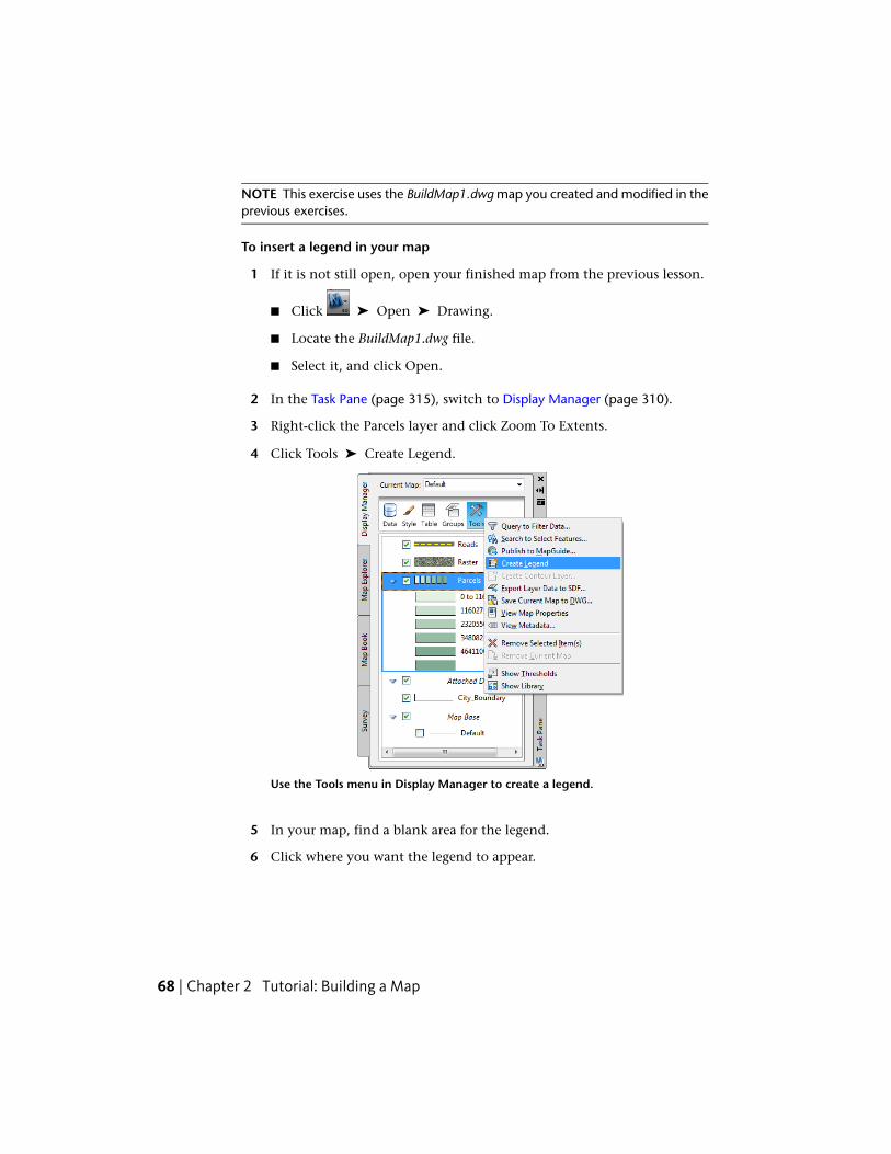
NOTE This exercise uses the BuildMap1.dwg map you created and modified in theprevious exercises.
To insert a legend in your map
1 If it is not still open, open your finished map from the previous lesson.
■ Click ➤ Open ➤ Drawing.
■ Locate the BuildMap1.dwg file.
■ Select it, and click Open.
2 In the Task Pane (page 315), switch to Display Manager (page 310).
3 Right-click the Parcels layer and click Zoom To Extents.
4 Click Tools ➤ Create Legend.
Use the Tools menu in Display Manager to create a legend.
5 In your map, find a blank area for the legend.
6 Click where you want the legend to appear.
68 | Chapter 2 Tutorial: Building a Map
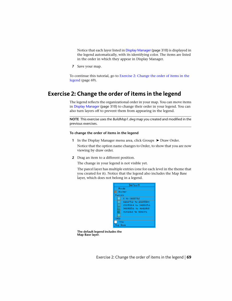
Notice that each layer listed in Display Manager (page 310) is displayed inthe legend automatically, with its identifying color. The items are listedin the order in which they appear in Display Manager.
7 Save your map.
To continue this tutorial, go to Exercise 2: Change the order of items in thelegend (page 69).
Exercise 2: Change the order of items in the legendThe legend reflects the organizational order in your map. You can move itemsin Display Manager (page 310) to change their order in your legend. You canalso turn layers off to prevent them from appearing in the legend.
NOTE This exercise uses the BuildMap1.dwg map you created and modified in theprevious exercises.
To change the order of items in the legend
1 In the Display Manager menu area, click Groups ➤ Draw Order.
Notice that the option name changes to Order, to show that you are nowviewing by draw order.
2 Drag an item to a different position.
The change in your legend is not visible yet.
The parcel layer has multiple entries (one for each level in the theme thatyou created for it). Notice that the legend also includes the Map Baselayer, which does not belong in a legend.
The default legend includes theMap Base layer.
Exercise 2: Change the order of items in the legend | 69
3 In Display Manager, clear the check box for the Map Base layer.
4 Click Tools ➤ Update Legend.
5 Save your map.
Where you are now
You inserted a legend, and then removed the reference to the Map Base layerfrom the legend. The legend now reflects the new organizational order.
To continue this tutorial, go to Lesson 8: Publish Your Map (page 70)
Lesson 8: Publish Your MapPublish a georeferenced map in DWF format, for eventual display on the Webor on an intranet. DWF (Design Web Format™) is an open, secure file formatdeveloped by Autodesk for sharing engineering design data. DWF files arehighly compressed, so they are smaller and quickly transmitted and viewed.This format can include object data or feature attributes, as well as the graphicalelements of your map.
If you assigned a coordinate system to all model-space maps in your DWF file,the publishing operation automatically converts the coordinate informationto latitude/longitude coordinates. Autodesk Design Review 2008 canautomatically navigate to a specific location when you enter coordinates. Itdisplays coordinates of any location in the map when you move your mouseover that location. With computers integrated with a GPS device using theNMEA 0183 protocol, field workers can center the map to coordinates providedby that device. As a result, the “my coordinates” icon appears within the map.
Files in DWF format can be displayed using Autodesk® Design Review. Forproduct information and a download link for this product, refer to theAutodesk Design Review page on the Autodesk web site. Autodesk DesignReview is the latest version of the Autodesk® DWF Viewer. It includes theability to measure, mark up, stamp, review, convert, and aggregate DWFcontent.
Exercise 1: Specify attributes to includeSet DWF publishing options that specify the attribute information to publishwith your map.
70 | Chapter 2 Tutorial: Building a Map
NOTE This exercise uses the BuildMap1.dwg map you created and modified in theprevious exercises.
To set publishing options
1 Open your finished map from the previous lesson.
■ Click ➤ Open ➤ Drawing.
■ Locate the BuildMap1.dwg file.
■ Select it, and click Open.
2 In the Tool-based Ribbon Workspace, click Output tab ➤ Export ToDWF/PDF panel ➤ Export To DWF/PDF Options (MAPDWFOPTIONS).
3 In the Map Information dialog box, select Publish Map Information.
4 In the Map Information dialog box, expand the items in the list andselect the Roads and Parcels items.
Exercise 1: Specify attributes to include | 71

You can include and exclude information at anylevel.
Notice that when you select Roads, everything under Roads isautomatically selected.
5 To publish the information to an XML file, click the file icon and specifya location for the published file. Click Save.
The DWF Publish operation uses the XML file.
6 Click OK.
To continue this tutorial, go to Exercise 2: Publish to DWF (page 72).
Exercise 2: Publish to DWFPublishing to DWF is like printing to a file. You set up plotting parameters,as if printing to a physical plotter. You apply those settings to your layout,which is like a plotting template. You display a layout tab for your map toactivate the layout.
72 | Chapter 2 Tutorial: Building a Map

Each view of your map (which initially includes model space and two defaultlayout spaces) is considered a sheet in your map sheet set. Learn more aboutsheet sets in the Help.
Use the Publish dialog box to specify the sheets to publish and whether topublish to a plotter or a file.
NOTE This exercise uses the BuildMap1.dwg map you created and modified in theprevious exercises.
To publish to DWF
1 Save your map.
You cannot plot or publish without saving first.
2 Click Output tab ➤ Plot panel ➤ Plot.
3 In the Plot dialog box, select a Printer/Plotter.
4 Click Apply To Layout, and then click Cancel.
Printer/plotter settings are applied to your publishing job without sendingthe job to a plotter or printer.
5 If Model and Layout tabs are not displayed just below your map,
right-click in the status area at the bottom of the application window.Click Display Model And Layout Tabs.
6 Click the Layout 1 tab.
7 Click ➤ Publish.
Do not choose an option from the Publish submenu. Click the wordPublish in the application menu.
8 In the Publish dialog box, in the Sheets To Publish list, make sure thatonly the sheets you want are selected.
For example, if another map is open, its model and layout views appearin the list. The default Layout2 view of the current map also appears.Select any undesired entries (such as Layout2) and click Remove Sheets.
9 Under Publish To, click DWF.
10 Click Publish Options and click Layer Information (under DWF DataOptions). On the pull-down menu in this field, click Include.
Exercise 2: Publish to DWF | 73

This setting publishes each layer in your map to a separate layer in DWF.In Design Review, you can turn the display of these layers on and offindependently.
11 Click OK to close the Publish Options dialog box.
12 In the Publish dialog box, click Publish (at the bottom of the window).
13 Specify a location and a name for the published file and click Select.
14 If you are prompted to save the sheet list, click No.
15 You might see a message telling you that the job is processing in thebackground. Click OK to dismiss the message.
The files needed by Autodesk Design Review are published to the file youspecified. Monitor the progress of the publishing operation by holdingyour cursor over the animated icon in the lower-right corner.
When the job is complete, a bubble appears in the bottom, right-handcorner of the window. Click the link in the bubble to view any warningsor errors. Close the window when you are done.
Where you are now
You have published your map to a DWF file, which can be displayed inAutodesk Design Review.
To continue this tutorial, go to Lesson 9: Branch Out - Find Data Sources (page74)
Lesson 9: Branch Out - Find Data SourcesAs you go on to create your own maps, you can add data to enhance them.For example, you can add surface rasters with elevation data for your area, orgeneric vector symbols showing parks, hydrants, or other items.
The Autodesk geodata portal has access to multiple data providers. In thislesson, you explore the geodata portal. Take a look at sample data providedwith AutoCAD Map 3D by the data providers who have partnered withAutodesk.
74 | Chapter 2 Tutorial: Building a Map

Exercise 1: Explore the Data Portal - DigitalGlobe®
In this exercise, you visit the geodata portal and view the data available fromDigitalGlobe®.®
To explore the DigitalGlobe data
1 In your browser, go to http://www.autodesk.com/geodata.
2 On the geodata site, click Go Now for DigitalGlobe.
3 Click the image of the Verrazano Narrows Bridge in Brooklyn, New Yorkto see the high-resolution satellite photo.
DigitalGlobe® has an exhaustive library of high-quality Earthimagery available for purchase.
4 To try out some of the DigitalGlobe data, click Download Your Free Trialand follow the directions on the screen.
Once you install DigitalGlobe and you start AutoCAD Map 3D, a newImageConnect menu appears on the menu bar.
To continue this lesson, go to Exercise 2: Explore the Data Portal - NAVTEQ™
(page 76).
Exercise 1: Explore the Data Portal - DigitalGlobe® | 75
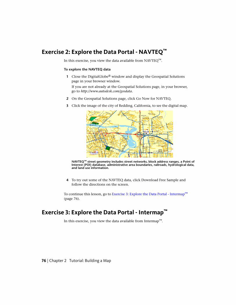
Exercise 2: Explore the Data Portal - NAVTEQ™
In this exercise, you view the data available from NAVTEQ™.
To explore the NAVTEQ data
1 Close the DigitalGlobe® window and display the Geospatial Solutionspage in your browser window.
If you are not already at the Geospatial Solutions page, in your browser,go to http://www.autodesk.com/geodata.
2 On the Geospatial Solutions page, click Go Now for NAVTEQ.
3 Click the image of the city of Redding, California, to see the digital map.
NAVTEQ™ street geometry includes street networks, block address ranges, a Point ofInterest (POI) database, administrative area boundaries, railroads, hydrological data,and land use information.
4 To try out some of the NAVTEQ data, click Download Free Sample andfollow the directions on the screen.
To continue this lesson, go to Exercise 3: Explore the Data Portal - Intermap™
(page 76).
Exercise 3: Explore the Data Portal - Intermap™
In this exercise, you view the data available from Intermap™.
76 | Chapter 2 Tutorial: Building a Map

To explore the Intermap data
1 Close the NAVTEQ™ window and display the Geospatial Solutions pagein your browser window.
If you are not already at the Geospatial Solutions page, in your browser,go to http://www.autodesk.com/geodata.
2 On the Geospatial Solutions page, click Go Now for Intermap.
3 Click the Digital Elevation Models image to see information about DEMtopographic layers.
Intermap™ provides digital surface models,digital terrain models, orthorectified radarimages, and color orthorectified radar images.
4 Close the browser windows.
To continue this lesson, go to Exercise 4: Try out the sample data (page 77).
Exercise 4: Try out the sample dataSample data from each of these providers is included with AutoCAD Map 3D.In this exercise, you add some of this data to a map of the city of Munich,Germany
Exercise 4: Try out the sample data | 77

To work with the sample data
1 Create a map.
■ Click ➤ New ➤ Drawing.
■ In the Open dialog box, select the map2d.dwt template.
■ In Map Explorer, right-click Current Drawing and click CoordinateSystem.
■ In the Assign Global Coordinate System dialog box, for Code, set thecoordinate system to LL84 and click OK.
2 Connect to a surface graphic.
■ In Display Manager, click Data ➤ Connect To Data.
■ In the Data Connect window, under Data Connections By Provider,click Add Raster Image or Surface Connection.
■ Click the file icon next to Source File Or Folder.
■ In the Open dialog box, navigate to the Intermap Munich_dtm.demraster file.
■ Select the file and click Open.
■ In the Data Connect window, click Connect.
■ In the Data Connect window, select the image and click Add To Map.
3 Style the surface image.
■ In Display Manager, select the surface layer.
■ On the status bar at the bottom of the application window, click thedown arrow next to Vertical Exaggeration.
■ Increase the vertical exaggeration to 25x.
■ In Display Manager, with the surface layer still selected, click Style.
■ In the Style Editor, click the down arrow in the Style cell and selectTheme.
■ In the Theme dialog box, under Specify A Theme, select Palette andselect the Contour Palette.
■ Click OK, then click Apply and close the Style Editor.
78 | Chapter 2 Tutorial: Building a Map
4 Connect to a satellite image of Munich.
■ If the Data Connect window is not displayed, in Display Manager,click Data ➤ Connect To Data.
■ In the Data Connect window, under Data Connections By Provider,click Add Raster Image or Surface Connection.
■ Click the file icon next to Source File Or Folder.
■ In the Open dialog box, navigate to the DigitalGlobe_munich.ecw rasterfile.
■ Select the file and click Open.
■ In the Data Connect window, click Connect.
■ In the Data Connect window, select the image and click Add To Map.
5 Style the satellite image.
■ In Display Manager, right-click the image layer and click Zoom ToExtents.
■ In Display Manager, with the image layer still selected, click Style.
■ In the Style Editor, click Transparent.
■ Click Select and select a dark gray color in the raster image to betransparent.
6 Connect to a Navteq SHP file to add points representing restaurants.
■ In Display Manager, click Data ➤ Connect To Data.
■ In the Data Connect window, under Data Connections By Provider,click Add SHP Connection.
■ In the Data Connect window, click the file icon next to Source FileOr Folder.
■ In the Open dialog box, navigate to the Navteq Restrnts.shp file.
■ Select the file and click Open.
■ In the Data Connect window, click Connect.
■ Select Restrnts and click Add To Map.
Exercise 4: Try out the sample data | 79
7 Style the points to use symbols.
■ In Display Manager, select the Restrnts layer and click Style.
■ In the Style Editor, click in the Style cell.
■ In the Style Point dialog box, click next to Symbol.
■ In the Select A Symbol dialog box, click next to Symbol Libraryand open the Map - Points of Interest.dwg file.
■ Select the Restaurant symbol.
■ If you want, in the Style Editor, change the Fill Color and Edge Colorof the points so you can see them better.
■ Click OK and close the Style Editor.
Where you are now
You explored the geodata portal. You used sample data from Autodesk partnerproviders to create a map of Munich using a surface with elevation, a satellitephoto, and symbols representing restaurants.
80 | Chapter 2 Tutorial: Building a Map

Exercise 4: Try out the sample data | 81

82
Tutorial: Moving FromAutoCAD to AutoCAD Map3D
About The AutoCAD/AutoCAD Map 3D TutorialAutoCAD Map 3D is built on AutoCAD and includes all AutoCAD functionality.Map files are saved in DWG format, just like regular AutoCAD drawings.However, AutoCAD Map 3D adds features that are not available in AutoCAD.Try out these additional features in this tutorial.
NOTE For a white paper by Russell Martin on the benefits of AutoCAD Map 3D toAutoCAD users, click here.
Lesson 1: Prepare Drawings for Use With AutoCADMap 3D
If you are new to AutoCAD Map 3D, your drawings might not be ready to takeadvantage of the features in AutoCAD Map 3D. This lesson covers some waysto prepare your data.
Digitize and georeference paper drawings
If your data is still stored in paper drawings, you can use AutoCAD Raster Designto digitize them and save them in AutoCAD drawing format.
3
83

You can also use AutoCAD Raster Design to georeference your data.Georeferencing aligns the drawing objects to real-world locations.Georeferenced drawings take advantage of many AutoCAD Map 3D features,such as combining data from multiple sources.
This tutorial does not cover the required steps in AutoCAD Raster Design todigitize and georeference drawings. Consult the AutoCAD Raster Designdocumentation for this information.
For more information about AutoCAD Raster Design, seehttp://www.autodesk.com/rasterdesign.
Set up a drive alias
When you edit drawings in AutoCAD Map 3D, others can work on those samedrawings at the same time. Individual objects are locked when you work onthem, so one person can edit part of a drawing while someone else works ona different section.
To use this feature, follow the procedures in this lesson to set up a drive alias.
Georeference existing drawings
To incorporate existing drawings into maps, the drawings must begeoreferenced. Otherwise, the drawing objects do not align with features inlarger maps.
Maps use coordinate systems to describe the position of objects using theirlongitude and latitude relative to a particular datum (an agreed-upon referencepoint). Once you assign a coordinate system to a map, you can add data tothat map from drawings that use different coordinate systems. AutoCAD Map3D automatically converts the data when you add it to the map, so everythinglines up.
However, if the incoming data does not have a coordinate system assigned toit, there is no way to convert it. Instead, designate the position of the datayourself.
This lesson shows you how to align objects in a non-georeferenced drawingwith features in a drawing with a known coordinate system.
Exercise 1: Set up a drive aliasA drive alias allows multiple users to use the same pathname for a drawingstored on a shared drive. It allows each user to map that drive to a differentdrive letter.
84 | Chapter 3 Tutorial: Moving From AutoCAD to AutoCAD Map 3D

To define a drive alias
1 In AutoCAD Map 3D, in the Task pane, click the Display Manager tab.
2 In Display Manager, click Data ➤ Add Drawing Data ➤ Attach SourceDrawings.
3 In the Define/Modify Drawing Set dialog box, click Attach.
4 In the Select Drawings to Attach dialog box, click (Create/Edit Aliases).
5 In the Drive Alias Administration dialog box, type a name for the alias.
The name must use only alphanumeric characters (including hyphenand underscore), contain no spaces or colons, and start with a character.For example, you can call the alias TutorialData.
6 Specify a path for the new alias.
In the Drive Alias Administration dialog box, specify a name for the alias and the actualpath it represents.
In this example, use the path to the folder where you copied your tutorialfiles.
7 Click Add, and then click Close.
Exercise 1: Set up a drive alias | 85
8 Click OK in the remaining two dialog boxes.
The drawing location is now mapped to your drive alias. You can nowopen drawings in that folder without defining any further aliases.
To continue this tutorial, go to Exercise 2: Georeference source drawings (page86).
Exercise 2: Georeference source drawingsYou can query objects from one drawing into another drawing of the samegeographical area, even if the drawings use different coordinate systems. Thequeried objects are automatically converted to the assigned coordinate system.If a drawing does not use a known coordinate system, align the objects to themap manually.
In this exercise, you georeference drawing objects by adding them to a mapwith a known coordinate system.
In practice, you can obtain such a map from the local county or municipality.For example, for a drawing of city parcels, obtain a digital version of an assessormap of that city. Make sure that you know the coordinate system used tocreate that map. We refer to this map as the “target map.” In this example,you connect to an SDF data store containing parcel information.
You use the Rubber Sheet command to align the drawing objects with knownlocations in the target map.
To georeference drawing objects
1 Create a drawing and assign a coordinate system.
■ Click ➤ New ➤ Drawing. Select the map2d.dwt template andclick Open.
■ Assign a coordinate system. Switch to Map Explorer in the Task Pane(page 315). Right-click Current Drawing and click Coordinate System.Enter CA-I and click OK.
2 Connect to a parcel data store of the same geographical area.
In this example, connect to the tutorial sample file PARCELS.SDF, whichuses the coordinate system CA-I.
■ Click Data ➤ Connect to Data.
86 | Chapter 3 Tutorial: Moving From AutoCAD to AutoCAD Map 3D
■ Under Data Connections By Provider, select Add SDF Connection.
■ Click the file icon next to Source File.
■ Navigate to the folder where you copied the sample files and selectPARCELS.SDF. Click Open.
■ Click Connect to add the parcel data file as a data source.
■ Under Add Data To Map, select Parcels.
■ Click Add To Map.
3 Open the drawing containing your drawing objects.
In this example, open the sample tutorial drawing subdivision_block.dwg,which has no coordinate system.
4 In the subdivision_block.dwg drawing, select and copy the objects to align.
The objects in subdivision_block.dwg are defined as a block.
■ Click anywhere on the block perimeter to select all the objects.
■ Click Home tab ➤ Clipboard panel ➤ Copy drop down ➤ Copy Clip
5 In the target map, paste the objects into the blank area in the center ofthe drawing.
■ Switch the current window to the parcels drawing you created.
■ Zoom into the large empty area in the center of the drawing.
■ In the empty area, right-click and select Paste.
■ Click an insertion point for the block.
Exercise 2: Georeference source drawings | 87

Paste the subdivision block in the empty space. Find the parcel to which the subdivisionaligns. In this illustration, the parcel is red (but it is not red in the sample file).
6 Find the points that the target map and the drawing objects have incommon.
For example, if your drawing represents new parcels, find the developmentthat contains those parcels. Find at least two common points.
In the parcels drawing you created, the parcel you want is to the left ofthe empty area. In the illustration above, it is red.
7 Use the Rubber Sheet command to align your drawing objects with theknown objects in the map.
■ Zoom in as close as you can, while still displaying the target area andthe subdivision drawing.
■ Click Tools tab ➤ Map Edit panel ➤ Rubber Sheet
■ When prompted on the command line for Base Point 1, click the firstcommon point in your drawing object block.
■ When prompted on the command line for Reference Point 1, clickthe corresponding point in the target map.
■ For this tutorial, specify four reference points. When you are finished,press Enter.
88 | Chapter 3 Tutorial: Moving From AutoCAD to AutoCAD Map 3D

The order in which you select the points and the spread of the pointsaffects the results. For complex curved figures, more vertices result ina more accurate alignment.
■ Select the object to align it with the reference area.
■ Enter s to select the objects to rubber sheet.
■ Click the subdivision block to select it.
■ Press Enter to complete the process.For more information about this procedure, and to see ananimation of the rubber sheet procedure, see Georeference parcelsby rubber sheeting.
Where you are now
You created a drive alias for drawings stored on a shared drive. Yougeoreferenced drawing objects, using the Rubber Sheet command to alignthem with known locations.
To continue this tutorial, go to Lesson 2: Clean Up Your Drawings (page 89).
Lesson 2: Clean Up Your DrawingsDrawings can contain various kinds of errors that make accurate mappingdifficult. For example, digitizing from a paper map can produce lines thatwere actually creases in the paper.
Drawings edited by multiple people can contain duplicate lines or objects.Finding duplicate objects in the same location can be nearly impossible withoutthe right tools.
If lines in your drawing do not connect precisely at endpoints, data thatappears to be precise can actually be inaccurate. Locating these issues visuallycan take hours.
AutoCAD Map 3D has an option called Drawing Cleanup to help you correctcommon geometry errors. In this lesson, you clean up a street map by deletingduplicate objects and extending undershoots. It is best to perform eachoperation separately, so you can see the result of each operation beforeperforming the next one.
Optionally, you can use a cleanup profile to automate the drawing cleanupprocess with scripts or to share settings with other users.
Lesson 2: Clean Up Your Drawings | 89
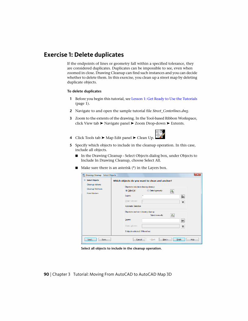
Exercise 1: Delete duplicatesIf the endpoints of lines or geometry fall within a specified tolerance, theyare considered duplicates. Duplicates can be impossible to see, even whenzoomed in close. Drawing Cleanup can find such instances and you can decidewhether to delete them. In this exercise, you clean up a street map by deletingduplicate objects.
To delete duplicates
1 Before you begin this tutorial, see Lesson 1: Get Ready to Use the Tutorials(page 1).
2 Navigate to and open the sample tutorial file Street_Centerlines.dwg.
3 Zoom to the extents of the drawing. In the Tool-based Ribbon Workspace,click View tab ➤ Navigate panel ➤ Zoom Drop-down ➤ Extents.
4 Click Tools tab ➤ Map Edit panel ➤ Clean Up.
5 Specify which objects to include in the cleanup operation. In this case,include all objects.
■ In the Drawing Cleanup - Select Objects dialog box, under Objects toInclude In Drawing Cleanup, choose Select All.
■ Make sure there is an asterisk (*) in the Layers box.
Select all objects to include in the cleanup operation.
90 | Chapter 3 Tutorial: Moving From AutoCAD to AutoCAD Map 3D
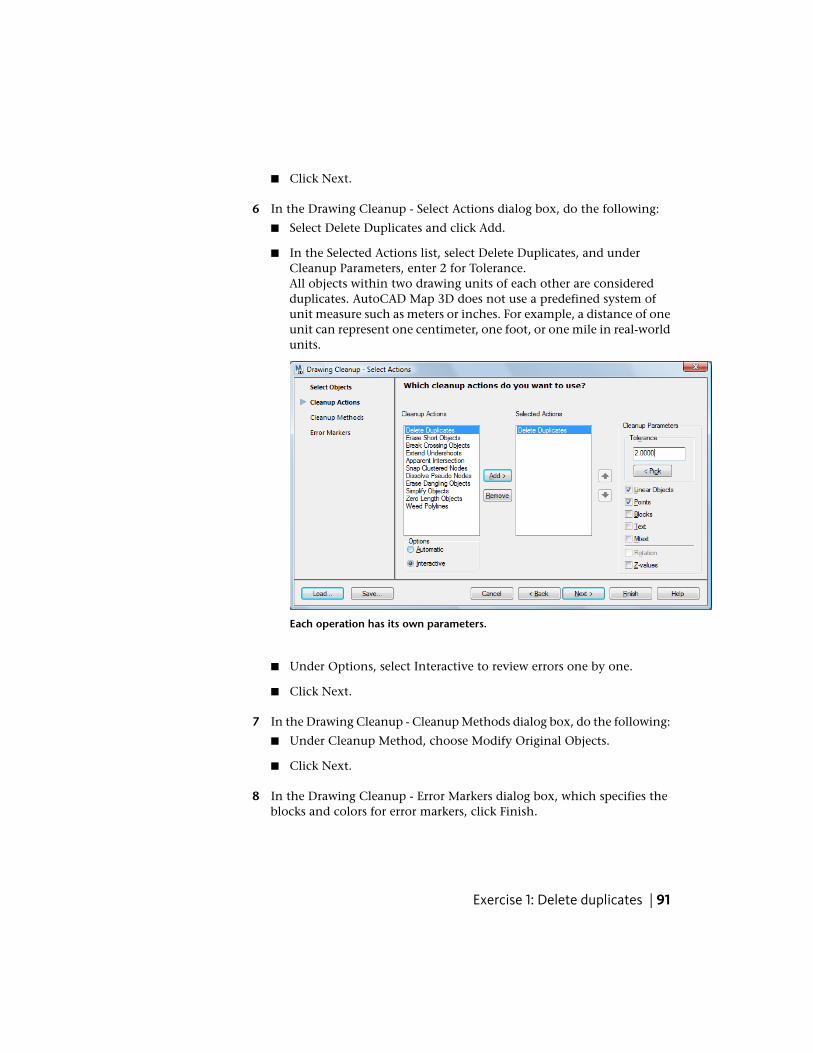
■ Click Next.
6 In the Drawing Cleanup - Select Actions dialog box, do the following:
■ Select Delete Duplicates and click Add.
■ In the Selected Actions list, select Delete Duplicates, and underCleanup Parameters, enter 2 for Tolerance.All objects within two drawing units of each other are consideredduplicates. AutoCAD Map 3D does not use a predefined system ofunit measure such as meters or inches. For example, a distance of oneunit can represent one centimeter, one foot, or one mile in real-worldunits.
Each operation has its own parameters.
■ Under Options, select Interactive to review errors one by one.
■ Click Next.
7 In the Drawing Cleanup - Cleanup Methods dialog box, do the following:
■ Under Cleanup Method, choose Modify Original Objects.
■ Click Next.
8 In the Drawing Cleanup - Error Markers dialog box, which specifies theblocks and colors for error markers, click Finish.
Exercise 1: Delete duplicates | 91

Drawing Cleanup locates the errors in the drawing and displays theDrawing Cleanup Errors dialog box. The dialog box groups the errors byerror type. Delete Duplicates is highlighted.
To review errors before fixing them, expand DeleteDuplicates. To fix all duplicates at once withoutreviewing them, select Delete Duplicates withoutexpanding it and click Fix All.
9 In the Drawing Cleanup Errors dialog box, do the following:
■ Expand Delete Duplicates to see how many duplicate objects weredetected.
■ Click Error 1 of 3.In the map, the first error displays a temporary marker so you canfind it easily.
92 | Chapter 3 Tutorial: Moving From AutoCAD to AutoCAD Map 3D

■ Click Fix to correct this error and proceed to the next error.
■ Continue clicking Fix until you have deleted all duplicate objects.
To continue this tutorial, go to Exercise 2: Extend undershoots (page 93).
Exercise 2: Extend undershootsUndershoots are objects that come within the specified tolerance radius ofeach other, but do not meet. Undershoots can occur due to inaccuratedigitizing or when converting scanned data. Use the Extend Undershootscleanup action to locate and correct undershoots.
If possible, one object is extended to cross the other. It maintains the samedirection and snaps to a point on the object. If no node exists, the operationcreates one at the intersection.
Two objects that pass within the specified tolerance snap together, as long asthe snap does not change their direction. If no node exists at that point, theoperation creates one.
NOTE This exercise uses the Street_Centerlines.dwg you used in Exercise 1: Deleteduplicates (page 90).
To extend undershoots
1 If the Street_Centerlines.dwg is not still open, reopen it.
2 Click Tools tab ➤ Map Edit panel ➤ Clean Up.
Exercise 2: Extend undershoots | 93

3 In the Drawing Cleanup - Select Objects dialog box, do the following:
■ Under Objects to Include In Drawing Cleanup, choose Select All.
■ Make sure there is an asterisk (*) in the Layers box.
■ Click Next.
Select all objects to include in the cleanup operation.
4 In the Drawing Cleanup - Select Actions dialog box, do the following:
■ Select Extend Undershoots and click Add.
■ In the Selected Actions list, select Extend Undershoots and enter 10for the Tolerance.
■ Under Options, select Interactive to review errors one by one.
■ Click Next.
5 In the Drawing Cleanup - Cleanup Methods dialog box, do the following:
■ Under Cleanup Method, choose Modify Original Objects.
■ Click Finish.
94 | Chapter 3 Tutorial: Moving From AutoCAD to AutoCAD Map 3D
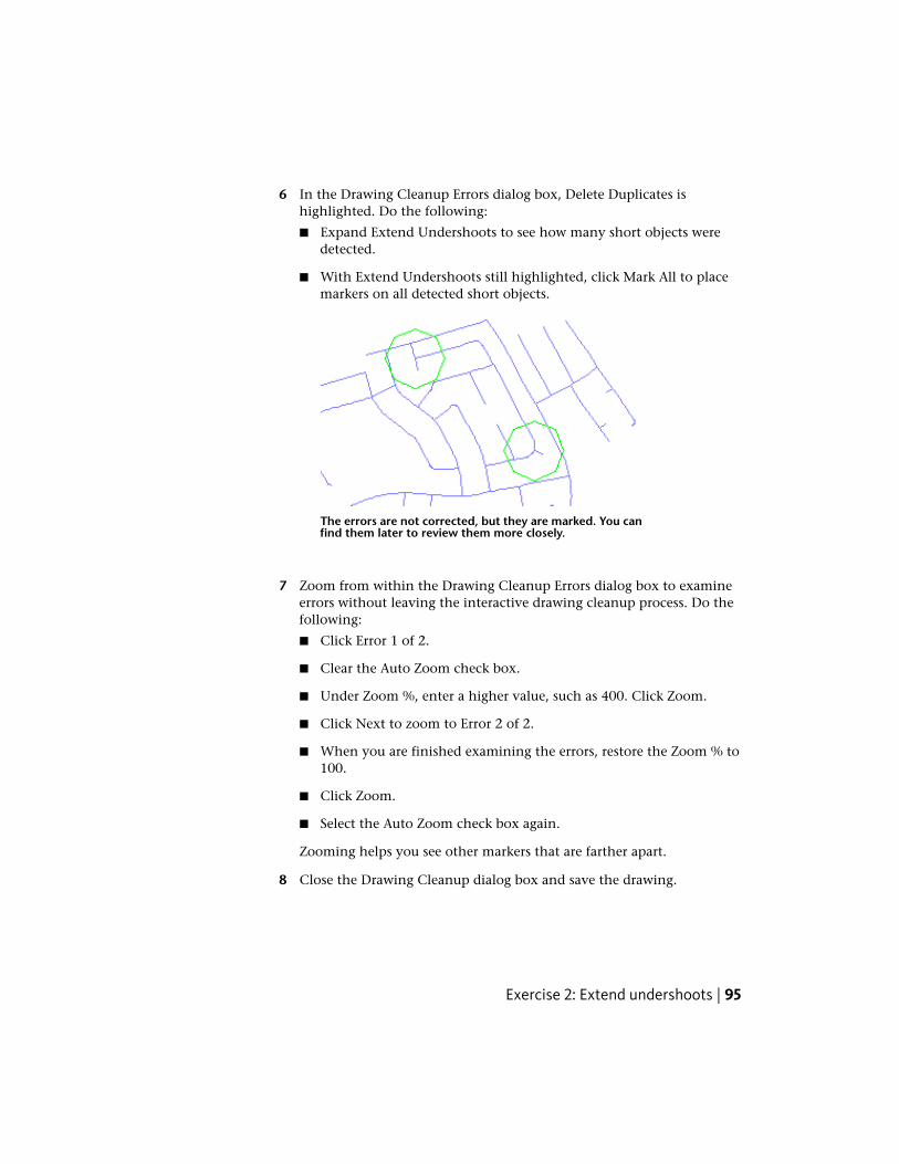
6 In the Drawing Cleanup Errors dialog box, Delete Duplicates ishighlighted. Do the following:
■ Expand Extend Undershoots to see how many short objects weredetected.
■ With Extend Undershoots still highlighted, click Mark All to placemarkers on all detected short objects.
The errors are not corrected, but they are marked. You canfind them later to review them more closely.
7 Zoom from within the Drawing Cleanup Errors dialog box to examineerrors without leaving the interactive drawing cleanup process. Do thefollowing:
■ Click Error 1 of 2.
■ Clear the Auto Zoom check box.
■ Under Zoom %, enter a higher value, such as 400. Click Zoom.
■ Click Next to zoom to Error 2 of 2.
■ When you are finished examining the errors, restore the Zoom % to100.
■ Click Zoom.
■ Select the Auto Zoom check box again.
Zooming helps you see other markers that are farther apart.
8 Close the Drawing Cleanup dialog box and save the drawing.
Exercise 2: Extend undershoots | 95

To continue this tutorial, go to Exercise 3: Use cleanup profiles (optional)(page 96).
Exercise 3: Use cleanup profiles (optional)You can save your settings for Drawing Cleanup in a profile and use themagain later. Profiles are useful when you automate the drawing cleanup processwith scripts or share settings with other users. Drawing Cleanup profiles aresaved as *.dpf files.
NOTE If you do not plan to use Drawing Cleanup profiles, you can skip this exerciseand go on to Lesson 3: Add Drawing Objects to a Map (page 98).
Drawing Cleanup profiles include all the options specified in the DrawingCleanup dialog boxes:
■ Layer names used for object selection
■ Cleanup actions and settings
■ Cleanup methods
■ Error marker settings (if any)
Drawing Cleanup profiles do not include the actual objects selected on thespecified layers.
In this exercise you create, save, and edit a Drawing Cleanup profile.
To create and save a Drawing Cleanup profile
1 Navigate to and open the tutorial sample file Street_Centerlines.dwg.
2 Click Tools tab ➤ Map Edit panel ➤ Clean Up.
3 In the Drawing Cleanup - Select Objects dialog box, do the following:
■ Under Objects To Include In Drawing Cleanup, make sure Select Allis selected.
■ Click Next.
4 In the Drawing Cleanup - Select Actions dialog box, do the following:
■ Under Cleanup Actions, select the actions for your profile.
96 | Chapter 3 Tutorial: Moving From AutoCAD to AutoCAD Map 3D

Select only Delete Duplicates. Since Drawing Cleanup is most effectivewhen each action is run separately, you can create a separate profilefor each action you use regularly.
■ Click Add to add Delete Duplicates to the Selected Actions window.
■ Click Save.
5 In the Save Drawing Cleanup Profile dialog box, enter a folder and aname for the profile.
For example, create a folder called DrawingCleanupProfiles and name thisprofile DeleteDuplicates.dpf.
6 Click Save As and specify a name and location.
7 Click Finish.
8 If the Drawing Cleanup Errors dialog box is displayed, click Cancel.
To use a saved profile
1 Open the drawing to clean.
NOTE Do not use the drawing you used in the previous exercises. It hasalready been corrected, so the loaded profile does not produce any furtherresults. If desired, replace that drawing with the original (uncorrected) sampledrawing from the installed tutorial sample data folder.
2 Click Tools tab ➤ Map Edit panel ➤ Clean Up.
3 In the Drawing Cleanup dialog box, click Load.
4 Select the profile and click Open.
5 In the Drawing Cleanup dialog box, click Finish.
6 Correct any errors.
Where you are now
You used the Drawing Cleanup option to remove duplicate lines and geometryand undershoots. You created a profile for use with other drawings.
To continue this tutorial, go to Lesson 3: Add Drawing Objects to a Map (page98).
Exercise 3: Use cleanup profiles (optional) | 97

Lesson 3: Add Drawing Objects to a MapWhen you add drawing objects to a map, you use a query (page 314) to specifythe objects you want. In this lesson, you add objects from multiple sourcedrawings to a single map. You use three types of queries:
■ Quick View — Displays all data in the attached drawings, but does notretrieve any objects. When you refresh the screen, the objects disappear.
■ Preview query mode — Displays objects in the attached drawings that matchcriteria you specify, but does not retrieve them. When you refresh the screen,the objects disappear.
■ Draw query mode — Retrieves objects that match criteria you specify(copies the objects into the current drawing). You can manipulate, edit,and save the objects (to their attached drawings, to the current drawing,or to a new drawing).
Attach multiple source drawings
Attaching a drawing to a map does not add any objects to the map. It makesthe drawing data available to the map. You can then preview or add the objects.
Preview drawing objects
Use Quick View or a Preview mode query to display objects in an attacheddrawing temporarily. For example, you can use a location preview query tosee all objects that fall within the radius of a circle that you draw.
These objects cross a circle in a location query.
98 | Chapter 3 Tutorial: Moving From AutoCAD to AutoCAD Map 3D

Use queries to add objects
Use Draw mode queries to retrieve information in attached drawing files andadd them to your drawing. In this lesson, you use two types of Draw modequeries:
■ Property queries — Retrieve objects based on properties such as color,linetype, or layer.
■ Location queries — Retrieve objects based on location conditions such asboundaries and buffer distances.
Alter object properties with a query
A special type of query allows you to alter the properties of the objects as youadd them to the map. For example, you can break out objects into layers,changing the layer property for the objects as you add them to your map.
Exercise 1: Attach source drawingsIn this exercise, you open a drawing for the city of Redding, California. Youattach three source drawings that contain parcel, sewer, and drainageinformation. Even though the drawings are attached, no objects appear untilyou perform a Quick View or a Preview mode query.
To attach drawings
1 If you have not already done so, see Lesson 1: Get Ready to Use theTutorials (page 1).
2 Navigate to and open the tutorial sample file Redding.dwg.
3 On the Map Explorer tab of the Task pane, right-click the Drawings folder.Click Attach.
Exercise 1: Attach source drawings | 99

Attach drawings from the Map Explorer tabof the Task pane.
4 In the Select Drawings to Attach dialog box, do the following:
■ Navigate to the location where you stored your tutorial sample files.
■ Press and hold the Ctrl key and select the following files: Drainage,Parcel, and Sewer.
■ Click Add.
■ Click OK.The parcel, sewer, and drainage drawings are now attached to theRedding.dwg file, but no drawing objects have been added yet.
To continue this tutorial, go to Exercise 2: Preview attached drawings withQuick View (page 100).
Exercise 2: Preview attached drawings with Quick ViewQuick View temporarily displays all data in the attached drawings in yourdrawing file. The drawing objects are not copied into the drawing.
NOTE This exercise uses the Redding.dwg map you created and modified in Exercise1: Attach source drawings (page 99).
100 | Chapter 3 Tutorial: Moving From AutoCAD to AutoCAD Map 3D
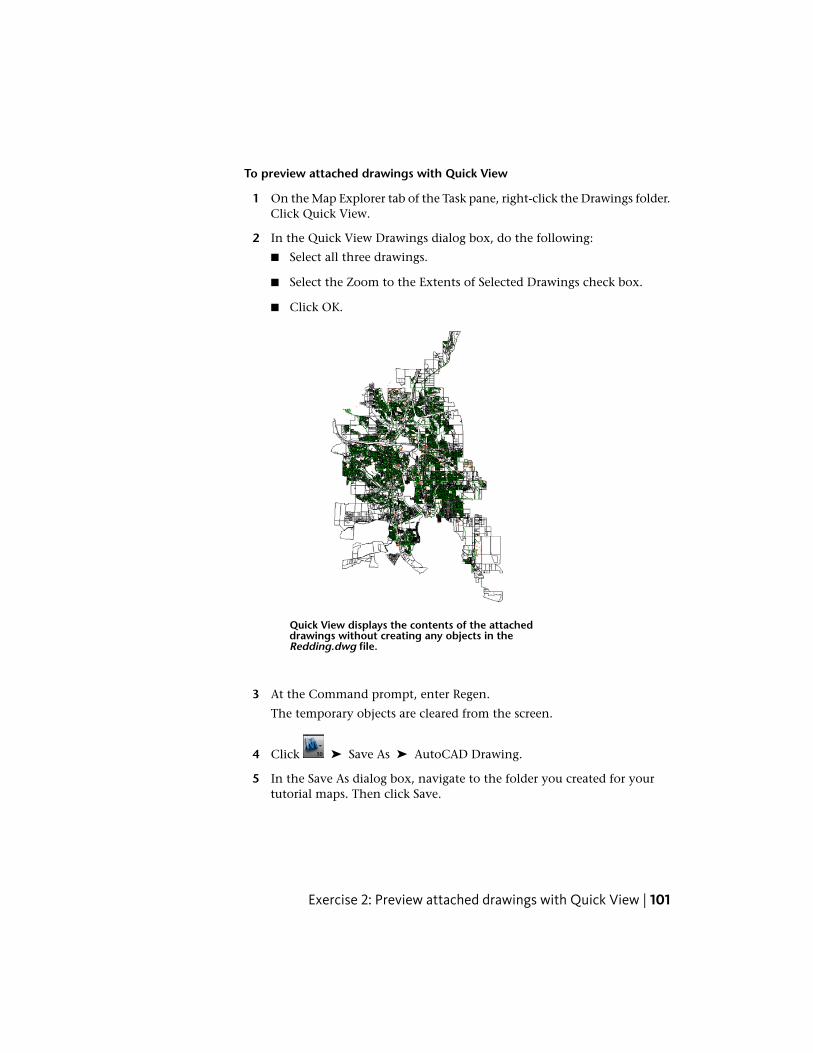
To preview attached drawings with Quick View
1 On the Map Explorer tab of the Task pane, right-click the Drawings folder.Click Quick View.
2 In the Quick View Drawings dialog box, do the following:
■ Select all three drawings.
■ Select the Zoom to the Extents of Selected Drawings check box.
■ Click OK.
Quick View displays the contents of the attacheddrawings without creating any objects in theRedding.dwg file.
3 At the Command prompt, enter Regen.
The temporary objects are cleared from the screen.
4 Click ➤ Save As ➤ AutoCAD Drawing.
5 In the Save As dialog box, navigate to the folder you created for yourtutorial maps. Then click Save.
Exercise 2: Preview attached drawings with Quick View | 101
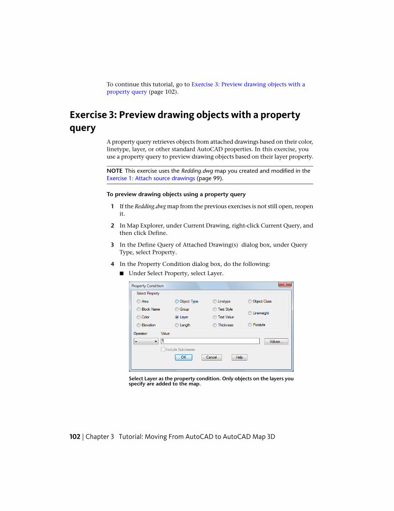
To continue this tutorial, go to Exercise 3: Preview drawing objects with aproperty query (page 102).
Exercise 3: Preview drawing objects with a propertyquery
A property query retrieves objects from attached drawings based on their color,linetype, layer, or other standard AutoCAD properties. In this exercise, youuse a property query to preview drawing objects based on their layer property.
NOTE This exercise uses the Redding.dwg map you created and modified in theExercise 1: Attach source drawings (page 99).
To preview drawing objects using a property query
1 If the Redding.dwg map from the previous exercises is not still open, reopenit.
2 In Map Explorer, under Current Drawing, right-click Current Query, andthen click Define.
3 In the Define Query of Attached Drawing(s) dialog box, under QueryType, select Property.
4 In the Property Condition dialog box, do the following:
■ Under Select Property, select Layer.
Select Layer as the property condition. Only objects on the layers youspecify are added to the map.
102 | Chapter 3 Tutorial: Moving From AutoCAD to AutoCAD Map 3D
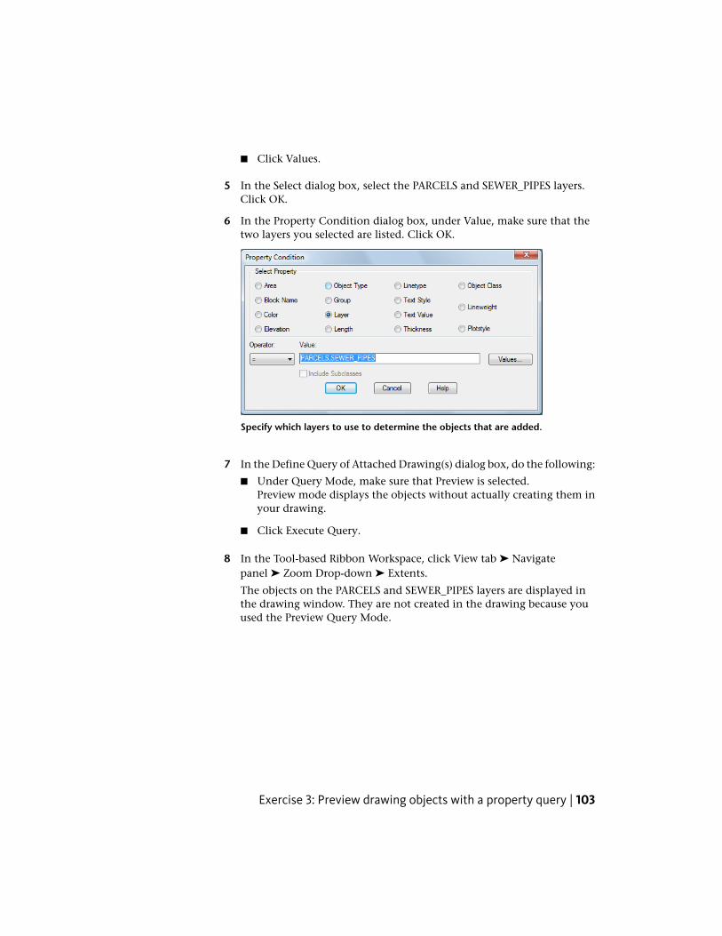
■ Click Values.
5 In the Select dialog box, select the PARCELS and SEWER_PIPES layers.Click OK.
6 In the Property Condition dialog box, under Value, make sure that thetwo layers you selected are listed. Click OK.
Specify which layers to use to determine the objects that are added.
7 In the Define Query of Attached Drawing(s) dialog box, do the following:
■ Under Query Mode, make sure that Preview is selected.Preview mode displays the objects without actually creating them inyour drawing.
■ Click Execute Query.
8 In the Tool-based Ribbon Workspace, click View tab ➤ Navigatepanel ➤ Zoom Drop-down ➤ Extents.
The objects on the PARCELS and SEWER_PIPES layers are displayed inthe drawing window. They are not created in the drawing because youused the Preview Query Mode.
Exercise 3: Preview drawing objects with a property query | 103
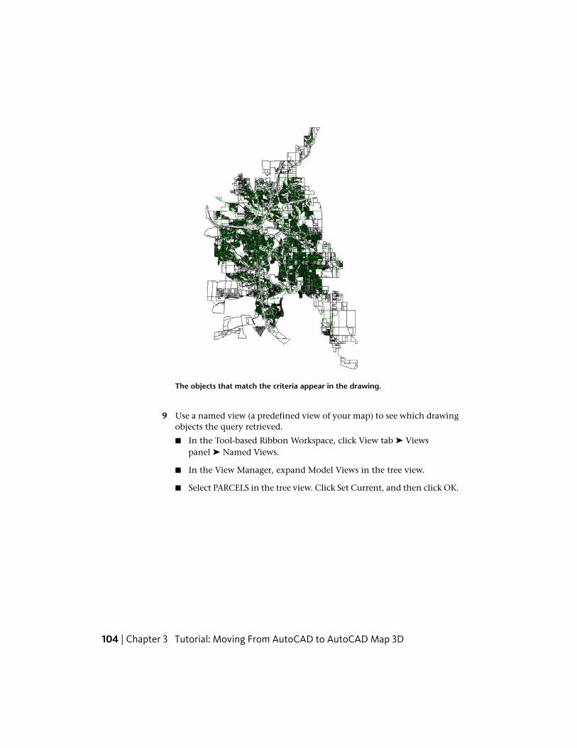
The objects that match the criteria appear in the drawing.
9 Use a named view (a predefined view of your map) to see which drawingobjects the query retrieved.
■ In the Tool-based Ribbon Workspace, click View tab ➤ Viewspanel ➤ Named Views.
■ In the View Manager, expand Model Views in the tree view.
■ Select PARCELS in the tree view. Click Set Current, and then click OK.
104 | Chapter 3 Tutorial: Moving From AutoCAD to AutoCAD Map 3D

Only the parcels (polygons with black outlines) and the sewerpipes (green lines) are displayed in the drawing area.
10 Do not save or close the drawing.
To continue this tutorial, go to Exercise 4: Retrieve objects with a propertyand location query (page 105).
Exercise 4: Retrieve objects with a property and locationquery
In this exercise, you add location conditions to the property query you definedin the previous exercise. Then you execute the result as a draw query to displaythe information in your drawing.
NOTE This exercise uses the Redding.dwg map you created and modified in Exercise1: Attach source drawings (page 99).
To combine location and property conditions in a query
1 In Map Explorer, under Current Drawing, right-click Current Query, andclick Define.
2 In the Define Query of Attached Drawing(s) dialog box, do the following:
■ Under Query Type, make sure And is selected.
■ Click Location.
3 In the Location Condition dialog box, do the following:
■ Under Boundary Type, select Circle.
Exercise 4: Retrieve objects with a property and location query | 105
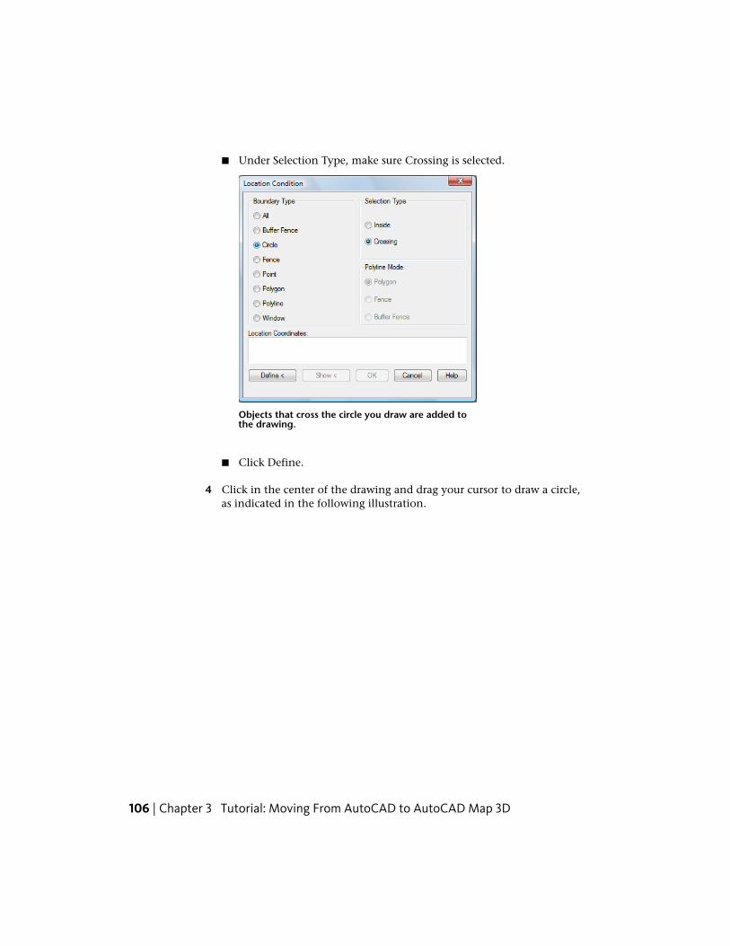
■ Under Selection Type, make sure Crossing is selected.
Objects that cross the circle you draw are added tothe drawing.
■ Click Define.
4 Click in the center of the drawing and drag your cursor to draw a circle,as indicated in the following illustration.
106 | Chapter 3 Tutorial: Moving From AutoCAD to AutoCAD Map 3D

Define the circle for the selection.
5 In the Define Query of Attached Drawing(s) dialog box, do the following:
■ Under Query Mode, select Draw.
■ Click Execute Query.
Exercise 4: Retrieve objects with a property and location query | 107
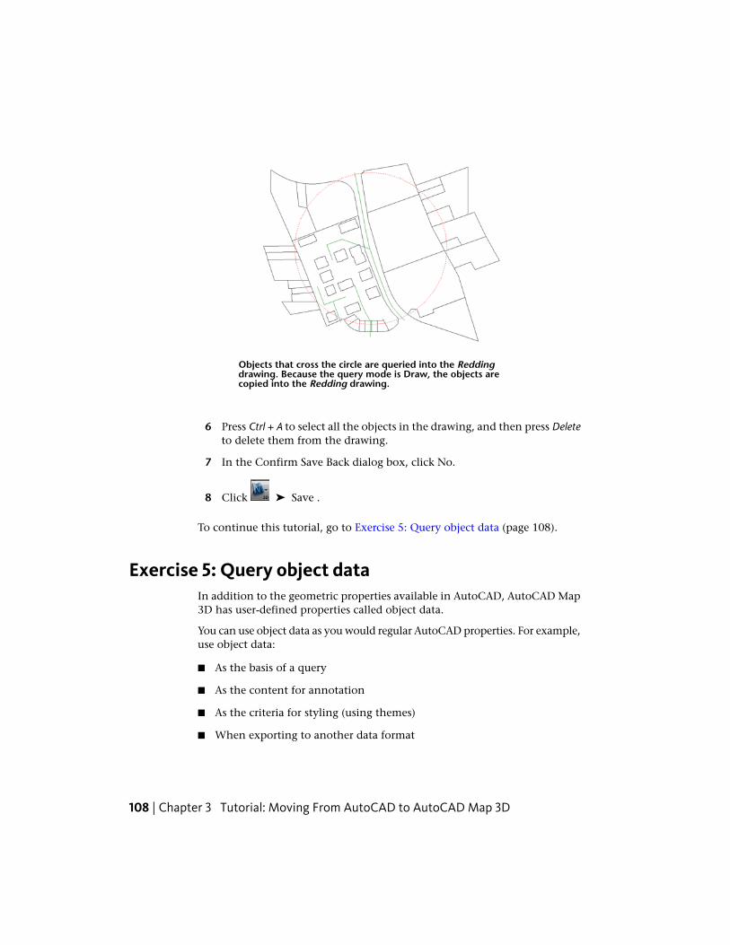
Objects that cross the circle are queried into the Reddingdrawing. Because the query mode is Draw, the objects arecopied into the Redding drawing.
6 Press Ctrl + A to select all the objects in the drawing, and then press Deleteto delete them from the drawing.
7 In the Confirm Save Back dialog box, click No.
8 Click ➤ Save .
To continue this tutorial, go to Exercise 5: Query object data (page 108).
Exercise 5: Query object dataIn addition to the geometric properties available in AutoCAD, AutoCAD Map3D has user-defined properties called object data.
You can use object data as you would regular AutoCAD properties. For example,use object data:
■ As the basis of a query
■ As the content for annotation
■ As the criteria for styling (using themes)
■ When exporting to another data format
108 | Chapter 3 Tutorial: Moving From AutoCAD to AutoCAD Map 3D
You must have AutoCAD Map 3D to create object data, but anyone who usesthe free Autodesk® Design Review software can view it. For example, a fieldworker can view a DWF™ version of a sewer map in Autodesk® Design Review.To see information about a sewer pipe, the worker holds the cursor over thatpipe. The information is available without obscuring the map itself.
The drawings in this tutorial have object data tables with information alreadyentered. In this exercise, you use object data (page 313) as a query condition.In a later exercise, you use object data to create feature classes in a new dataformat.
NOTE This exercise uses the Redding.dwg map you created and modified in Exercise1: Attach source drawings (page 99).
To create a query based on object data
1 If the Redding.dwg map from the previous exercise is not still open, reopenit.
2 In Map Explorer, under Current Drawing, right-click Current Query, andclick Define.
3 In the Define Query of Attached Drawing(s) dialog box, do the following:
■ Under Current Query, click Clear Query.
■ Under Query Type, click Data.
4 In the Data Condition dialog box, do the following:
■ Select Object Data.
■ Under Tables, select SEWER_PIPES.
■ Under Object Data Fields, select PIPESIZE.
■ In the Expression area, under Operator, select >. Under Value, enter8.
Exercise 5: Query object data | 109
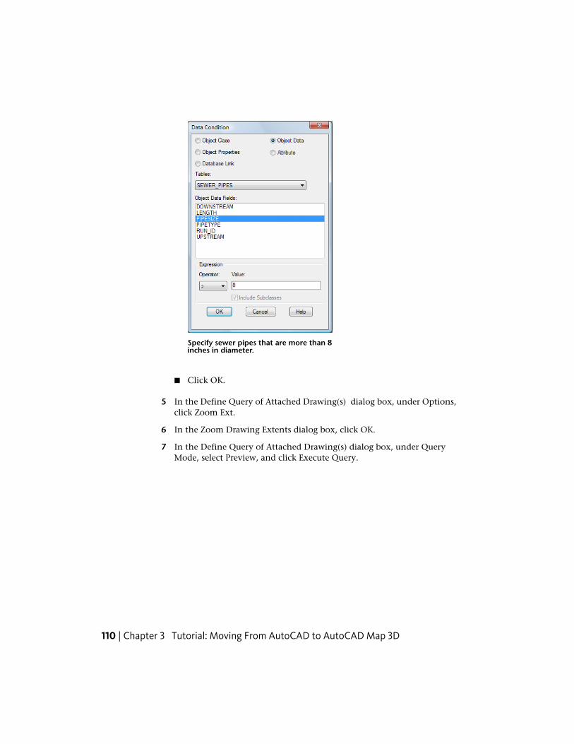
Specify sewer pipes that are more than 8inches in diameter.
■ Click OK.
5 In the Define Query of Attached Drawing(s) dialog box, under Options,click Zoom Ext.
6 In the Zoom Drawing Extents dialog box, click OK.
7 In the Define Query of Attached Drawing(s) dialog box, under QueryMode, select Preview, and click Execute Query.
110 | Chapter 3 Tutorial: Moving From AutoCAD to AutoCAD Map 3D
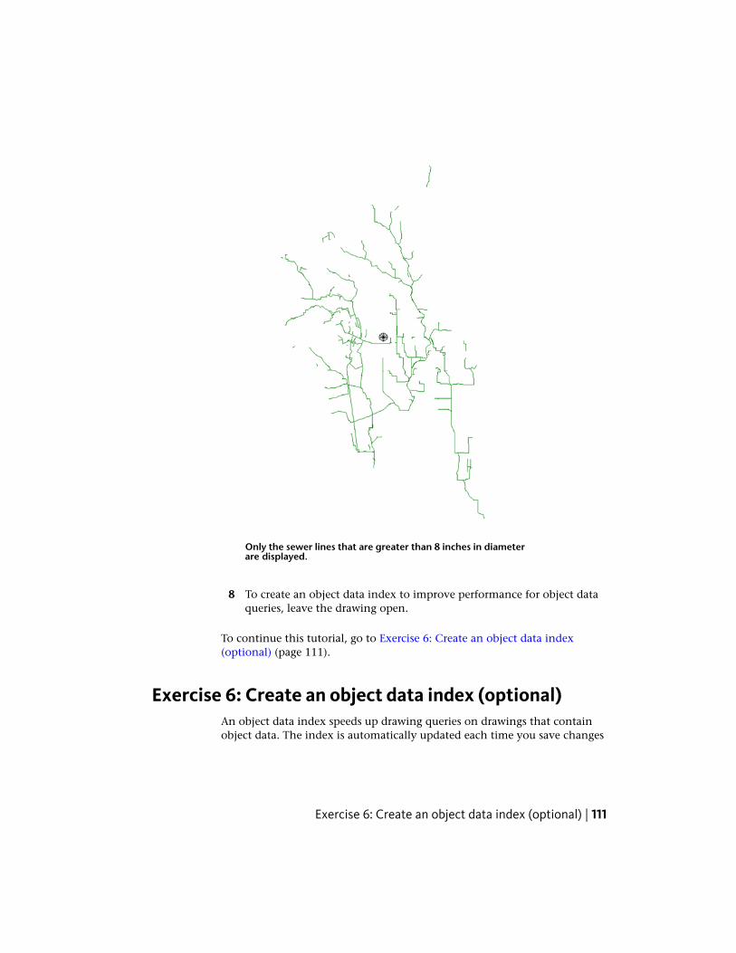
Only the sewer lines that are greater than 8 inches in diameterare displayed.
8 To create an object data index to improve performance for object dataqueries, leave the drawing open.
To continue this tutorial, go to Exercise 6: Create an object data index(optional) (page 111).
Exercise 6: Create an object data index (optional)An object data index speeds up drawing queries on drawings that containobject data. The index is automatically updated each time you save changes
Exercise 6: Create an object data index (optional) | 111
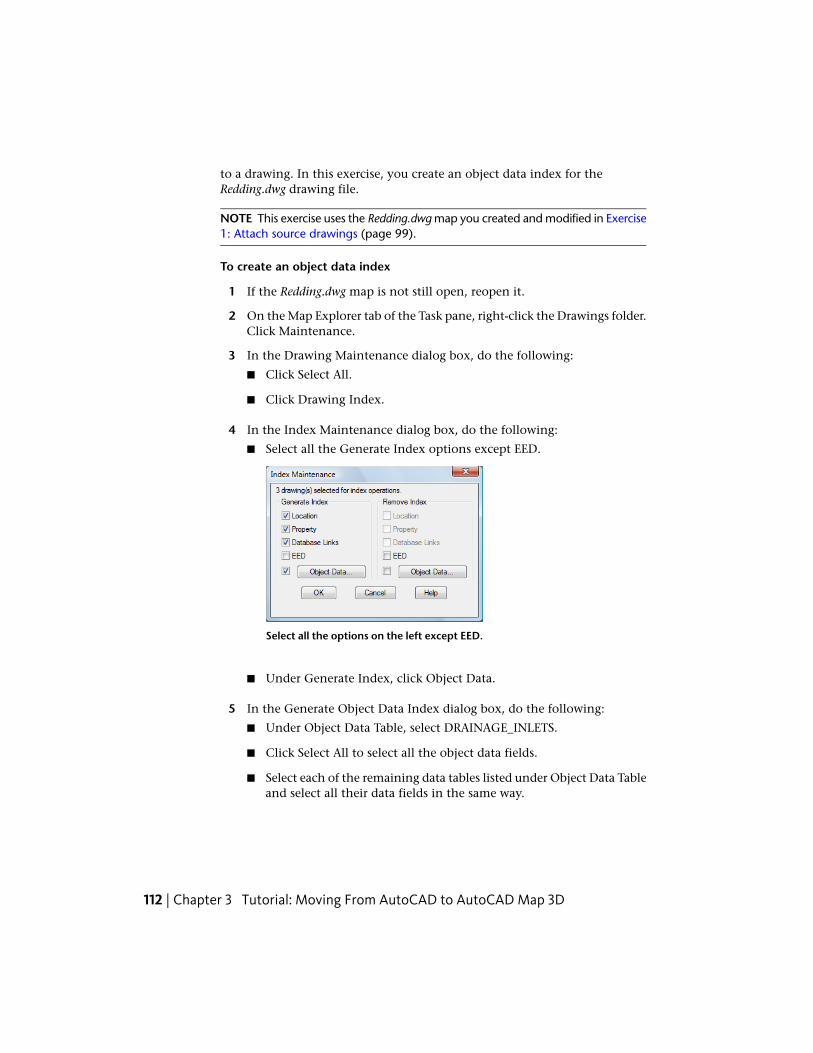
to a drawing. In this exercise, you create an object data index for theRedding.dwg drawing file.
NOTE This exercise uses the Redding.dwg map you created and modified in Exercise1: Attach source drawings (page 99).
To create an object data index
1 If the Redding.dwg map is not still open, reopen it.
2 On the Map Explorer tab of the Task pane, right-click the Drawings folder.Click Maintenance.
3 In the Drawing Maintenance dialog box, do the following:
■ Click Select All.
■ Click Drawing Index.
4 In the Index Maintenance dialog box, do the following:
■ Select all the Generate Index options except EED.
Select all the options on the left except EED.
■ Under Generate Index, click Object Data.
5 In the Generate Object Data Index dialog box, do the following:
■ Under Object Data Table, select DRAINAGE_INLETS.
■ Click Select All to select all the object data fields.
■ Select each of the remaining data tables listed under Object Data Tableand select all their data fields in the same way.
112 | Chapter 3 Tutorial: Moving From AutoCAD to AutoCAD Map 3D

Select a data table, then select its datafields.
■ Click OK when you are finished.
6 In the Index Maintenance dialog box, click OK.
7 In the Confirm dialog box, click OK.
8 In the Drawing Maintenance dialog box, click Close.
The indexes are created. As you work with your drawings, repeat thisprocedure periodically to update and recreate the indexes.
9 Click ➤ Save .
Where you are now
You used Quick View and Preview queries to look at objects in attacheddrawings. You used Draw queries to add objects from attached drawings tothe current drawing. You created an object data index to improve theperformance of data queries.
To see the effect of the object index on performance, repeat Exercise 5: Queryobject data (page 108) with the new index you just created.
To continue this tutorial, go to Lesson 4: Add Raster Images (page 114).
Exercise 6: Create an object data index (optional) | 113

Lesson 4: Add Raster ImagesMaps can contain more than drawing objects. For example, you can addgraphics.
In this lesson, you insert a raster (bitmapped) graphic and display it behindthe other objects in your map.
You also modify the image in your map. Your edits do not change the originalimage file, but only the way the map displays it. In this lesson, you changethe brightness and contrast. You also clip the image, to display only part ofit.
NOTE For a tutorial on adding an FDO raster image through Data Connect, seeExercise 5: Add a raster image (page 45) in the Building a Map tutorial.
Exercise 1: Insert a raster imageAerial and satellite photographs often contain information about their locationand scale. This information makes the images “georeferenced.” AutoCADcannot use this georeferencing information, so it cannot properly positionthe imagery, but AutoCAD Map 3D can.
In this exercise, you insert a digital raster graphic (DRG) of Redding, California,into a drawing of the same city. The information in the associated TIFF worldfile (TWF) allows you to locate and scale the image correctly.
NOTE While it is not required for this tutorial, you can download AutoCAD RasterDesign Object Enabler for AutoCAD Map 3D 2009 fromhttp://www.autodesk.com/rasterobjenabler. This free utility supports many rasterimage formats that Data Connect does not support.
114 | Chapter 3 Tutorial: Moving From AutoCAD to AutoCAD Map 3D

Raster images provide context for drawing objects, like roads.
To insert a raster image
1 If you have not already done so, see Lesson 1: Get Ready to Use theTutorials (page 1).
2 Open the tutorial sample file CITY.dwg.
3 Click Home tab ➤ Data panel ➤ Insert An Image.
4 In the Insert Image dialog box, do the following:
■ Navigate to the location where you stored your tutorial sample files.
■ In the Files Of Type box, select Tagged Image File Format (*.tif,*.tiff).
■ In the list of images, select REDDING_DRG.tif.
■ Click Information to display the file size, creation date, and otherinformation, as well as a preview of the image.
Exercise 1: Insert a raster image | 115
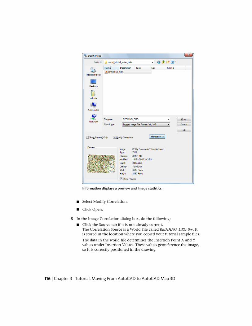
Information displays a preview and image statistics.
■ Select Modify Correlation.
■ Click Open.
5 In the Image Correlation dialog box, do the following:
■ Click the Source tab if it is not already current.The Correlation Source is a World File called REDDING_DRG.tfw. Itis stored in the location where you copied your tutorial sample files.
The data in the world file determines the Insertion Point X and Yvalues under Insertion Values. These values georeference the image,so it is correctly positioned in the drawing.
116 | Chapter 3 Tutorial: Moving From AutoCAD to AutoCAD Map 3D

NOTE You can manually adjust the insertion values as needed.
■ Click OK.The image is correctly placed in the drawing.
6 Save the file.
■ Click ➤ Save As ➤ AutoCAD Drawing.
■ In the Save As dialog box, navigate to the folder you created for yourtutorial maps.
■ Click Save.
To continue this tutorial, go to Exercise 2: View image information (page 117).
Exercise 2: View image informationYou can view the file name, size, density, depth, and type for an image youinserted. You can also view the date the image was created and modified, andthe layer on which it resides.
In this exercise, you view information about the raster image in two ways.The second method displays some additional information, such as the widthand height of the image.
NOTE This exercise uses the CITY.dwg map you used in Exercise 1: Insert a rasterimage (page 114).
To view information about a raster image
1 If the CITY.dwg map is not still open, reopen it.
2 In the drawing area, place your cursor over the image, hold down theShift key and click the image.
3 Click Insert tab ➤ Image panel ➤ Image Management.
4 In the Image Management dialog box, view information about theREDDING_DRG image.
Exercise 2: View image information | 117
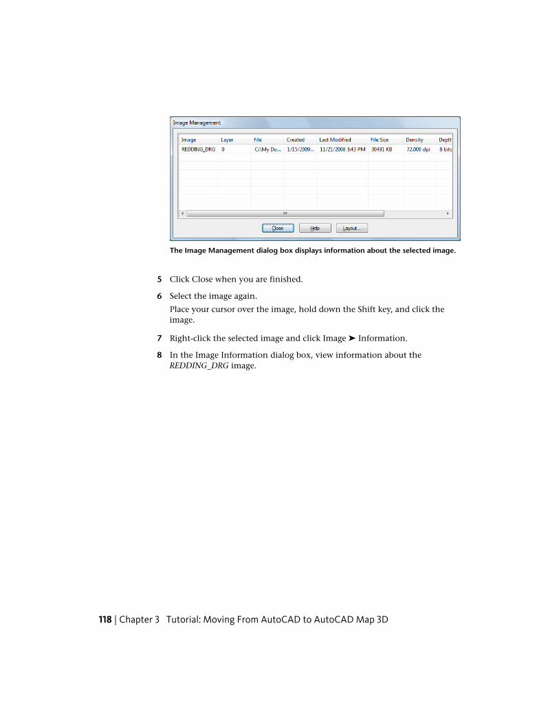
The Image Management dialog box displays information about the selected image.
5 Click Close when you are finished.
6 Select the image again.
Place your cursor over the image, hold down the Shift key, and click theimage.
7 Right-click the selected image and click Image ➤ Information.
8 In the Image Information dialog box, view information about theREDDING_DRG image.
118 | Chapter 3 Tutorial: Moving From AutoCAD to AutoCAD Map 3D

The Image Information dialog box has some extra imageinformation.
9 Click Close when you are finished.
To continue this tutorial, go to Exercise 3: Change the display order (page 119).
Exercise 3: Change the display orderIn this exercise, you change the display order of the raster image in the drawingfile. You send the raster image to the back, so objects in the original mapdisplay in front of it.
NOTE This exercise uses the CITY.dwg map you used in Exercise 1: Insert a rasterimage (page 114).
To change the display order
1 If the CITY.dwg map is not still open, reopen it.
2 In the drawing area, place your cursor over the image, hold down theShift key, and click the image.
Exercise 3: Change the display order | 119
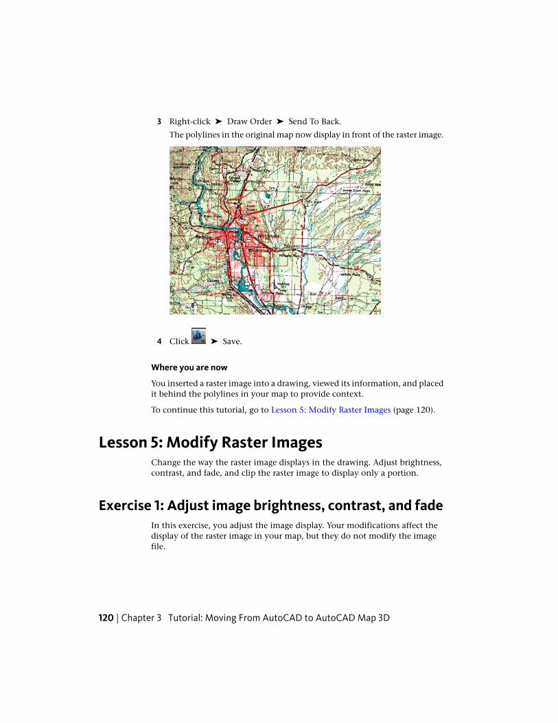
3 Right-click ➤ Draw Order ➤ Send To Back.
The polylines in the original map now display in front of the raster image.
4 Click ➤ Save.
Where you are now
You inserted a raster image into a drawing, viewed its information, and placedit behind the polylines in your map to provide context.
To continue this tutorial, go to Lesson 5: Modify Raster Images (page 120).
Lesson 5: Modify Raster ImagesChange the way the raster image displays in the drawing. Adjust brightness,contrast, and fade, and clip the raster image to display only a portion.
Exercise 1: Adjust image brightness, contrast, and fadeIn this exercise, you adjust the image display. Your modifications affect thedisplay of the raster image in your map, but they do not modify the imagefile.
120 | Chapter 3 Tutorial: Moving From AutoCAD to AutoCAD Map 3D
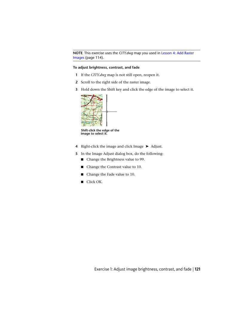
NOTE This exercise uses the CITY.dwg map you used in Lesson 4: Add RasterImages (page 114).
To adjust brightness, contrast, and fade
1 If the CITY.dwg map is not still open, reopen it.
2 Scroll to the right side of the raster image.
3 Hold down the Shift key and click the edge of the image to select it.
Shift-click the edge of theimage to select it.
4 Right-click the image and click Image ➤ Adjust.
5 In the Image Adjust dialog box, do the following:
■ Change the Brightness value to 99.
■ Change the Contrast value to 10.
■ Change the Fade value to 10.
■ Click OK.
Exercise 1: Adjust image brightness, contrast, and fade | 121

The image is much lighter, displaying the polylines of theoriginal map more clearly.
6 Click ➤ Save.
To continue this tutorial, go to Exercise 2: Clip the image (page 122).
Exercise 2: Clip the imageIn this exercise, you change the width of the polyline that represents the citylimits. The city limits display more prominently in the drawing. Then youclip the image to display a rectangular portion that frames the city .
NOTE This exercise uses the CITY.dwg map you used in Exercise 1: Adjust imagebrightness, contrast, and fade (page 120).
To change the width of a polyline
1 If the CITY.dwg map is not still open, reopen it.
2 Move your cursor over the city limits.
122 | Chapter 3 Tutorial: Moving From AutoCAD to AutoCAD Map 3D

The green polyline represents thecity limits.
3 Click the polyline to select it.
If the Quick Properties panel is not displayed, right-clickanywhere in the drawing and select Quick Properties.
4 Move your cursor over the Quick Properties window to expand it.
The Global Width property becomes visible.
5 Select the value for Global Width, enter 100, and press Enter.
You can edit values in the QuickProperties window.
6 Press Esc to close the Quick Properties window.
Exercise 2: Clip the image | 123
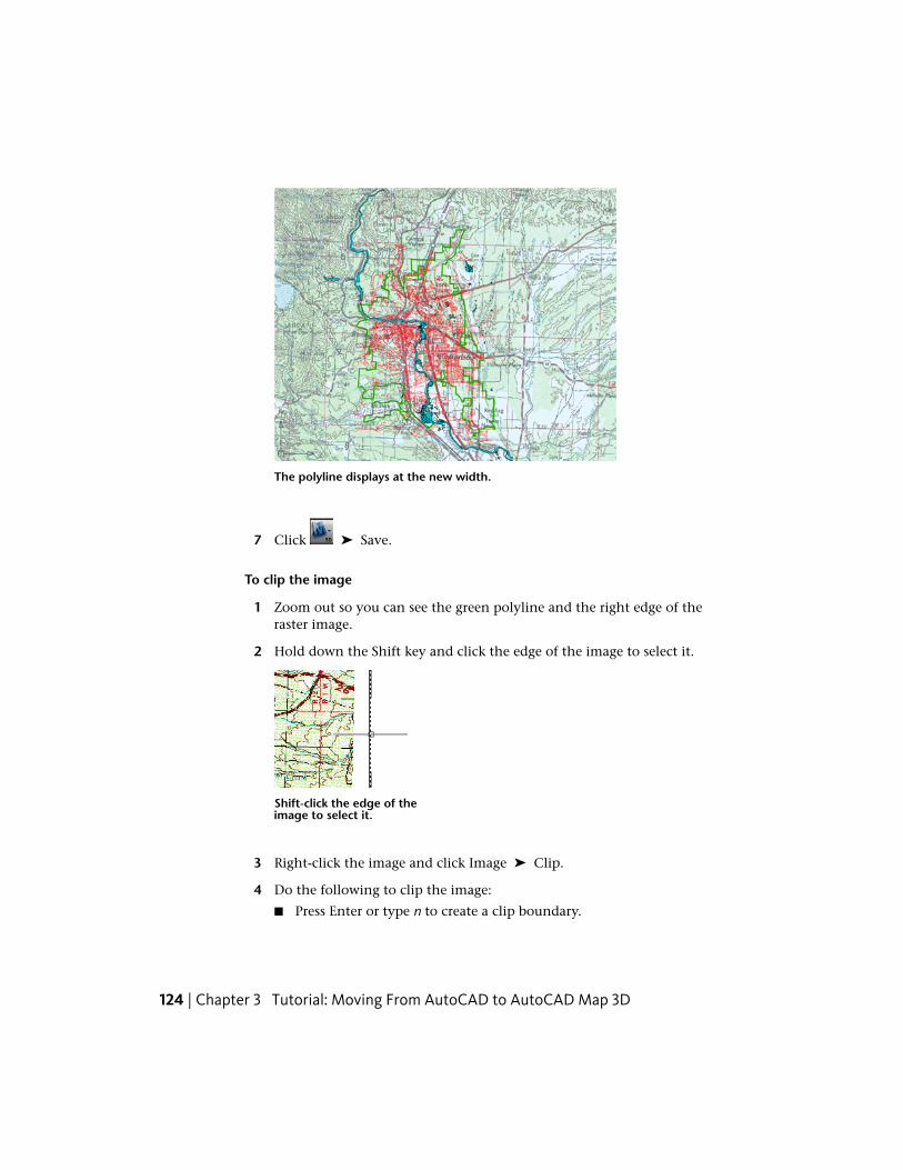
The polyline displays at the new width.
7 Click ➤ Save.
To clip the image
1 Zoom out so you can see the green polyline and the right edge of theraster image.
2 Hold down the Shift key and click the edge of the image to select it.
Shift-click the edge of theimage to select it.
3 Right-click the image and click Image ➤ Clip.
4 Do the following to clip the image:
■ Press Enter or type n to create a clip boundary.
124 | Chapter 3 Tutorial: Moving From AutoCAD to AutoCAD Map 3D
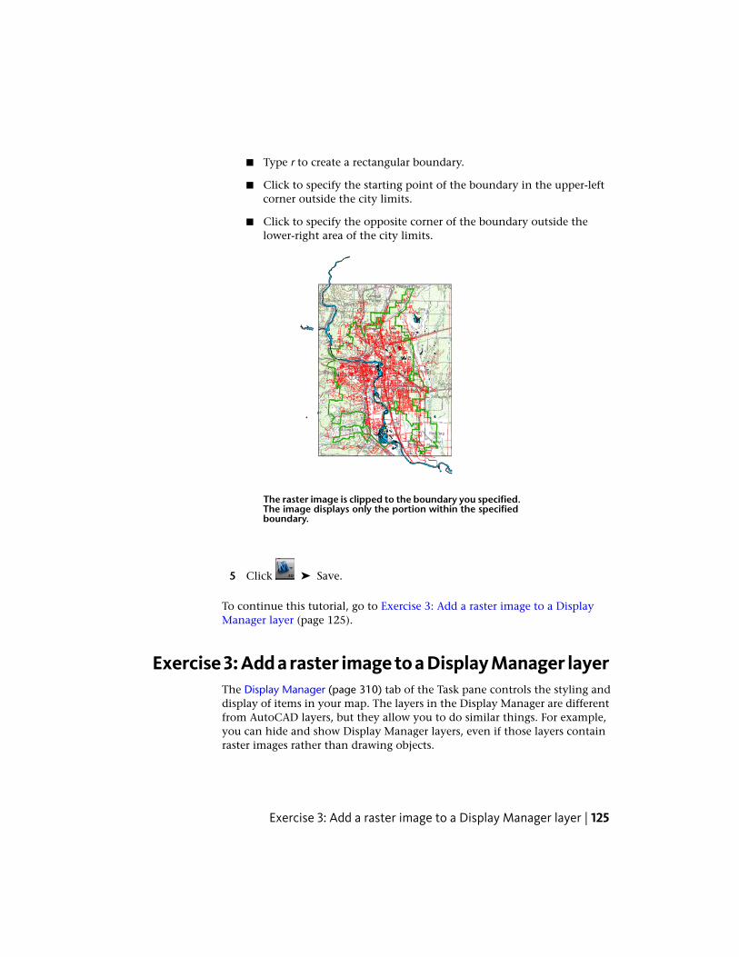
■ Type r to create a rectangular boundary.
■ Click to specify the starting point of the boundary in the upper-leftcorner outside the city limits.
■ Click to specify the opposite corner of the boundary outside thelower-right area of the city limits.
The raster image is clipped to the boundary you specified.The image displays only the portion within the specifiedboundary.
5 Click ➤ Save.
To continue this tutorial, go to Exercise 3: Add a raster image to a DisplayManager layer (page 125).
Exercise 3: Add a raster image to a Display Manager layerThe Display Manager (page 310) tab of the Task pane controls the styling anddisplay of items in your map. The layers in the Display Manager are differentfrom AutoCAD layers, but they allow you to do similar things. For example,you can hide and show Display Manager layers, even if those layers containraster images rather than drawing objects.
Exercise 3: Add a raster image to a Display Manager layer | 125

In this lesson, you add a raster image to a Display Manager layer. You renameand hide the raster image layer.
NOTE This exercise uses the CITY.dwg map you used in Exercise 1: Adjust imagebrightness, contrast, and fade (page 120).
To add an image to a new Display Manager layer
1 If the CITY.dwg map is not still open, reopen it.
2 On the Display Manager tab of the Task pane, click Data ➤ Add DrawingData ➤ Raster Image.
3 In the Select Image dialog box, select the check box next toREDDING_DRG.
4 Click OK.
In the Display Manager, REDDING_DRGis now listed as a layer.
5 In the Display Manager, right-click the REDDING_DRG layer and clickRename.
6 Type REDDING_RASTER and press Enter.
7 Click ➤ Save.
8 In the Display Manager, clear the check box for the REDDING_RASTERlayer.
126 | Chapter 3 Tutorial: Moving From AutoCAD to AutoCAD Map 3D

The raster image is no longer displayed in the drawing.
Where you are now
You adjusted the image appearance in your map without changing the imagefile itself. You added the image to a layer in Display Manager, where you canhide and show it easily.
To continue this tutorial, go to Lesson 6: Share Your Map with Others (page127).
Lesson 6: Share Your Map with OthersYou can convert your drawing objects to a geospatial format using the Exportoption.
For example, you can export your map to an Autodesk SDF file. This storesthe geometry for each drawing object as data, so it can be shared with otherAutodesk users in a small, portable format. When you connect to that file inAutoCAD Map 3D, all the objects appear on the screen, like AutoCAD objects.
Lesson 6: Share Your Map with Others | 127

You can edit them using the same commands. However, the objects are now“features” and are stored in a data file, rather than in an AutoCAD drawing.
You can also publish your map to a DWF file. People without a copy ofAutoCAD Map 3D can view this format using a free, downloadable vieweravailable from http://www.autodesk.com/designreview.
Exercise 1: Export a map to Autodesk SDFThe drawing you used in Lesson 2: Clean Up Your Drawings (page 89) containsobject data (page 313). Object data consists of attributes of the real-world objectsthat the drawing objects represent. The object data is stored in the map itselfand is associated with individual drawing objects.
When you export drawing objects, you can use object data to create featureclasses in an SDF file. The resulting feature classes have properties thatcorrespond to the object data attributes.
In this exercise, the street centerlines in the drawing have three object dataattributes: Lanes, Speed_Limit, and Surface.
To export drawing objects to SDF
1 Navigate to and open the Street_Centerlines.dwg map you used in Lesson2: Clean Up Your Drawings (page 89).
2 Click Output tab ➤ Map Data Transfer panel ➤ Map 3D Export.
3 In the Export Location dialog box, do the following:
■ Make sure Files Of Type is set to Autodesk SDF (*.SDF).
■ Specify a location and a file name for the exported file.
■ Click OK.
4 In the Export dialog box, on the Selection tab, make sure Select All isselected.
5 Click the Feature Class tab, and do the following:
■ Click Create Multiple Classes Based On A Drawing Object.
■ For Drawing Object To Use, select Object Data.
■ Under Drawing Object, clear the Non-Classified check box.
128 | Chapter 3 Tutorial: Moving From AutoCAD to AutoCAD Map 3D
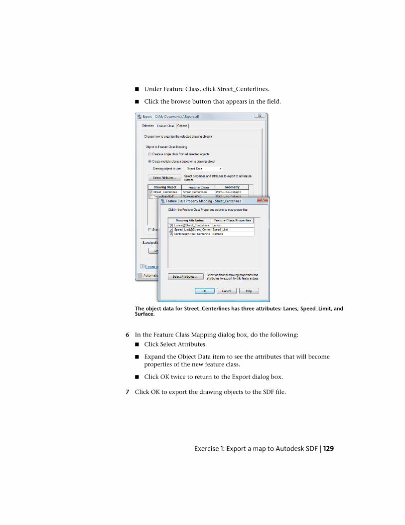
■ Under Feature Class, click Street_Centerlines.
■ Click the browse button that appears in the field.
The object data for Street_Centerlines has three attributes: Lanes, Speed_Limit, andSurface.
6 In the Feature Class Mapping dialog box, do the following:
■ Click Select Attributes.
■ Expand the Object Data item to see the attributes that will becomeproperties of the new feature class.
■ Click OK twice to return to the Export dialog box.
7 Click OK to export the drawing objects to the SDF file.
Exercise 1: Export a map to Autodesk SDF | 129
Use the Data Connect window to connect to the resulting SDF file. To see ananimation on how to do this, see Exercise 2: Use Data Connect to add datato your map (page 32) in the “Introducing AutoCAD Map 3D 2010” tutorial.
You can edit the features in the SDF file using AutoCAD commands.
To continue this tutorial, go to Exercise 2: Publish a map to a DWF file (page130).
Exercise 2: Publish a map to a DWF fileIn this exercise, you set DWF publishing options that specify the object datato publish with your map. Then you publish your map to a DWF file.
NOTE This exercise uses the Street_Centerlines.dwg map you modified in Lesson2: Clean Up Your Drawings (page 89).
To set publishing options
1 Navigate to and open the Street_Centerlines.dwg map you used in Lesson2: Clean Up Your Drawings (page 89).
2 Click Output tab ➤ Export To DWF/PDF panel ➤ DWF Options.
3 In the Map Information dialog box, select Publish Map Information.
4 In the Map Information dialog box, expand the items in the list andselect Street_Centerlines.
130 | Chapter 3 Tutorial: Moving From AutoCAD to AutoCAD Map 3D
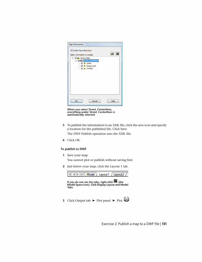
When you select Street_Centerlines,everything under Street_Centerlines isautomatically selected.
5 To publish the information to an XML file, click the save icon and specifya location for the published file. Click Save.
The DWF Publish operation uses the XML file.
6 Click OK.
To publish to DWF
1 Save your map.
You cannot plot or publish without saving first.
2 Just below your map, click the Layout 1 tab.
If you do not see the tabs, right-click (theModel Space icon). Click Display Layout and ModelTabs.
3 Click Output tab ➤ Plot panel ➤ Plot.
Exercise 2: Publish a map to a DWF file | 131

4 In the Plot dialog box, under Printer/Plotter, select DWF6eplot.pc3.
5 Click Apply To Layout, and then click Cancel.
Printer/plotter settings are applied to your publishing job without sendingthe job to a plotter or printer.
6 Click ➤ Publish.
NOTE Do not choose an option from the Publish submenu. Click the wordPublish in the application menu.
7 In the Publish dialog box, do the following:
■ in the Sheets To Publish list, make sure that only the sheets you wantare selected.For example, if another map is open, its model and layout views appearin the list. The default Layout2 view of the current map also appears.
Select any undesired entries (such as Layout2) and click .
■ Under Publish To, select DWF .
■ Click Publish Options.
8 In the Publish Options dialog box, do the following:
■ Click Layer Information (under General DWF/PDF Options).
■ On the pull-down menu in this field, click Include.Each layer in your map becomes a separate layer in the DWF output.In Design Review, you can turn the display of these layers on and offindependently.
■ Click OK.
9 In the Publish dialog box, do the following:
■ Click Publish (at the bottom of the window).
■ Specify a location and a name for the published file and click Select.
■ If you are prompted to save the sheet list, click No.
10 If you see a message about the job processing in the background, clickClose to dismiss the message.
The files needed by Autodesk Design Review are published to the file youspecified.
132 | Chapter 3 Tutorial: Moving From AutoCAD to AutoCAD Map 3D
11 Monitor the progress of the publishing operation by holding your cursorover the animated icon in the lower-right corner.
12 When the job is complete, a bubble appears in the bottom, right-handcorner of the window. Click the link in the bubble to view any warningsor errors. Close the window when you are finished.
Where you are now
You exported your map to an Autodesk SDF file. You also published your mapto a DWF file. People without a copy of AutoCAD Map 3D can view yourpublished map using a free, downloadable viewer available fromhttp://www.autodesk.com/designreview.
Exercise 2: Publish a map to a DWF file | 133

134
Tutorial: ClassifyingDrawing Objects
About the Classifying Drawing Objects TutorialIn this tutorial, you define object classes, assign drawing objects to differentclasses, and then use the object classes to create, edit, and export drawing objects.To be part of the object class, drawing objects must meet certain rules whenthey are classified. If you create a drawing object in an object class, it inheritsthe layer and attribute characteristics of that object class. Object classes help toensure that drawing objects are standardized.
For example, you can define an object class (page 313) called Roads and specifyits rules:
■ It can contain only line objects.
■ All members of the Roads class have a property for number of lanes.
■ The value for the Lanes property is from 1 through 6.
Then, only line objects that represent 1- to 6-lane roads can be added to theRoads class.
Object classification is helpful when you create metadata. Although the AutoCADMap 3D Metadata feature generates basic metadata for DWG files, it is optimizedfor use with maps that use object classes.
Object classification is useful when you are preparing drawing files for exportto a spatial data (FDO) format, such as SDF or Oracle. You can export objectsbased on object classes. Then, each set of exported objects has only the propertiesassigned to it by its object class.
4
135
NOTE This tutorial is for DWG data only. Geospatial data uses feature classesinstead of object classes, and feature classes are defined in the data store itself.
Using Industry Toolkits to Set Up Classification
The AutoCAD Map 3D Industry Toolkits provide industry-specific data modelsand templates for water, wastewater, and electric utilities. The Industry Toolkitsinclude object class definitions and supporting material specific to eachindustry. Data in DWG or other file formats can be easily classified to matchIndustry Toolkit object classes.
The toolkits include:
■ Data modelsA set of industry object classes and corresponding data attributes, forexample, an overhead conductor and the voltage carried by that conductor.
■ A set of pre-configured industry symbols that are tied to the object classes.
■ Templates for AutoCAD Map 3D maps (DWT files) and object classification(XML files).
■ Documentation (a User’s Guide, Workflows, and Data Model Schemas).
■ Instructional videos
The AutoCAD Map 3D Industry Toolkits are provided as free downloads toAutoCAD Map 3D 2010 Subscription customers. In North America, the toolkitsare available from within Subscription Center athttp://www.autodesk.com/subscriptioncenter.
The AutoCAD Map 3D Industry Toolkits are for use only with licensedAutoCAD Map 3D software. The toolkits are subject to the terms and conditionsof the Autodesk Software License Agreement that accompanies that licensedsoftware.
Lesson 1: Set Up For ClassificationTo use this tutorial, prepare the sample data, change your AutoCAD Map 3Dworkspace, and set up your user privileges (page 316) for AutoCAD Map 3D.
136 | Chapter 4 Tutorial: Classifying Drawing Objects

Exercise 1: Set up your work environmentCopy the sample data to a local drive and switch to the Tool-Based Ribbonworkspace.
1 Prepare your sample data. (page 2)
2 Create a folder for your saved maps. (page 3)
3 Start AutoCAD Map 3D.
4 Switch to the Tool-based Ribbon workspace. (page 4)
To continue this tutorial, go to Exercise 2: Set up your user privileges (page137).
Exercise 2: Set up your user privilegesYou must have the appropriate user privileges (page 316) to define object classes(page 313) for your version of AutoCAD Map 3D.
Creating a User with the Required Privileges
If your organization does not assign privileges, you can log in as SuperUser(page 315). As SuperUser, you can create a user with the privileges you need.
NOTE If your organization assigns user privileges for AutoCAD Map 3D, ask theSuperUser in your group to grant you these privileges.
To log in as SuperUser
1 Click Map Setup tab ➤ Map panel ➤ ➤ User Login.
2 Do one of the following:
■ If you have not changed the SuperUser login, specify the default loginname SuperUser and the password SUPERUSER, using the capitalizationshown. (Login is case sensitive.)
Exercise 1: Set up your work environment | 137
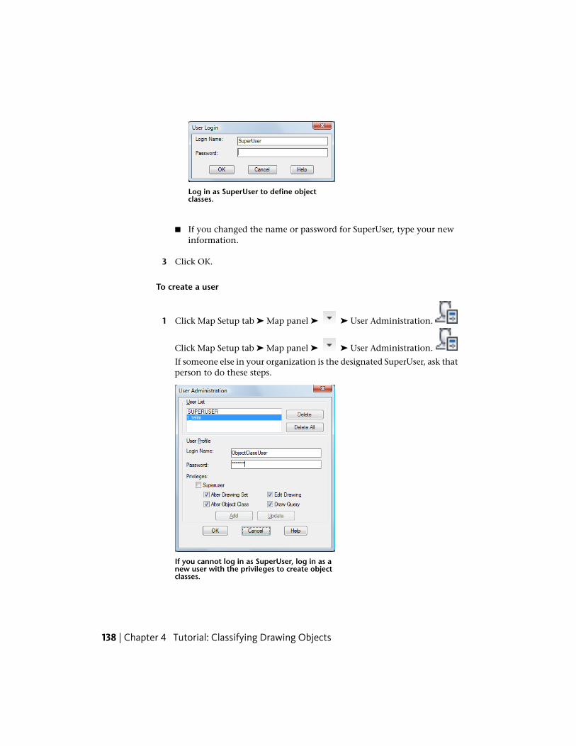
Log in as SuperUser to define objectclasses.
■ If you changed the name or password for SuperUser, type your newinformation.
3 Click OK.
To create a user
1 Click Map Setup tab ➤ Map panel ➤ ➤ User Administration.
Click Map Setup tab ➤ Map panel ➤ ➤ User Administration.
If someone else in your organization is the designated SuperUser, ask thatperson to do these steps.
If you cannot log in as SuperUser, log in as anew user with the privileges to create objectclasses.
138 | Chapter 4 Tutorial: Classifying Drawing Objects

2 Specify a new user name and password.
3 Assign all privileges except SuperUser to the new user and click OK.
Where you are now
You set up the privileges necessary for creating object class definitions.
To continue this tutorial, go to Lesson 2: Define Object Classes (page 139).
Lesson 2: Define Object ClassesYou define object classes by example. You select an existing object thatembodies the object class (page 313) you are defining (a “model object”). Thenyou modify the properties for that object to define the class.
Object class definitions are stored in an object class definition (page 313) file,which you can attach to any map. You can add definitions from multipledrawings to a single definition file. It becomes a library of object classes. Youattach the definition file to a map. Then you use the object classes in thatdefinition file to classify existing objects and create new ones.
Exercise 1: Create the object class definition fileUse the Map Explorer tab in the Task pane to create the object class definition(page 313) file. You can create this file in any map.
To create the definition file
1 Click ➤ New ➤ Drawing.
Select the map2d.dwt template and click Open.
2 Switch to Map Explorer in the Task pane.
3 Right-click Object Classes and click New Definition File.
Lesson 2: Define Object Classes | 139

Create the object class definitionfile.
NOTE If you see an error message, you are not logged in as a user who candefine object classes. See Exercise 2: Set up your user privileges (page 137).
4 Name and save the definition file in a convenient location.
For example, navigate to the folder where you copied your tutorial files.Call the definition file MyDefinition.xml.
5 Right-click Object Classes again and click Attach Definition File. Specifythe definition file you created.
Object classes you define are now saved in the new definition file.
To continue this tutorial, go to Exercise 2: Define an object class (page 140).
Exercise 2: Define an object classYou must base each new object class (page 313) on an existing object. Start byopening a map that contains objects that are typical of the object class youare defining (“model objects”). In this example, you open the Roads.dwg mapto define the Roads object class.
140 | Chapter 4 Tutorial: Classifying Drawing Objects
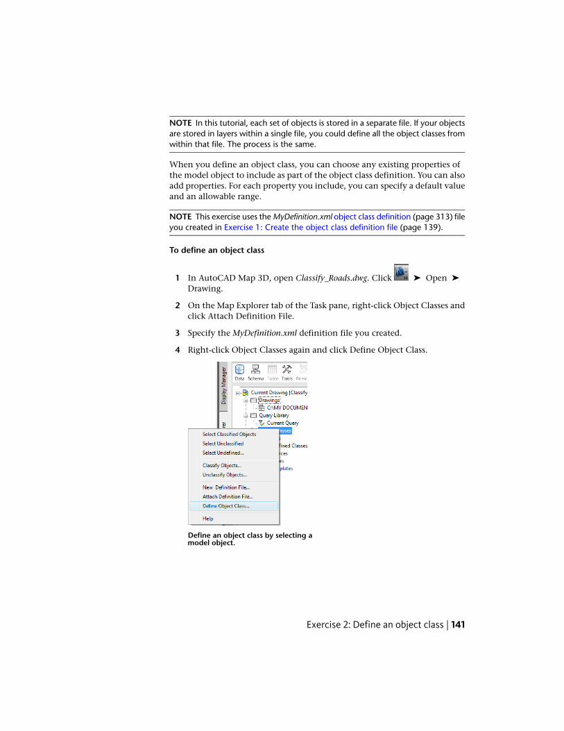
NOTE In this tutorial, each set of objects is stored in a separate file. If your objectsare stored in layers within a single file, you could define all the object classes fromwithin that file. The process is the same.
When you define an object class, you can choose any existing properties ofthe model object to include as part of the object class definition. You can alsoadd properties. For each property you include, you can specify a default valueand an allowable range.
NOTE This exercise uses the MyDefinition.xml object class definition (page 313) fileyou created in Exercise 1: Create the object class definition file (page 139).
To define an object class
1 In AutoCAD Map 3D, open Classify_Roads.dwg. Click ➤ Open ➤
Drawing.
2 On the Map Explorer tab of the Task pane, right-click Object Classes andclick Attach Definition File.
3 Specify the MyDefinition.xml definition file you created.
4 Right-click Object Classes again and click Define Object Class.
Define an object class by selecting amodel object.
Exercise 2: Define an object class | 141

5 Select any road as the model object for this class. Click Map Setup
tab ➤ Object Class panel ➤ Define.
6 In the Define Object Classification dialog box, specify Roads as the namefor this object class. Click the topmost box in the Object Types list(AcDbEntity).
Specify the object creation method that existing objects mustuse to belong to this object class.
All existing objects you add to this class must use the object type (page313) you check here. Unless you know for certain that all existing roadobjects were created using the AcDbLine or AcDbCurve method, it is saferto check only AcDbEntity (page 309).
7 Click the Properties List tab and check the properties to include in thisobject class.
Objects you include in this class always retain their own properties. Theproperties you specify here are the properties of the class as a whole.Choose properties to set their default values or allowable ranges, or tomake them editable for all members of the class.
142 | Chapter 4 Tutorial: Classifying Drawing Objects

For example, to be able to change the layer, linetype, or color for allmembers of the Roads class as a group, select those properties. You canset default values, where appropriate. For example, you can assign allmembers of the Roads class to a Roads layer.
You can include the following property types:
■ General properties, such as color and layer
■ Miscellaneous properties, such as linetype generation
■ Object properties, such as street name (ST_NAME).
Specify the properties for objects in this object class, and anydefault values for those properties.
The following table shows a suggested set of General properties and valuesfor the Roads class.
ValueProperty
General Properties
RedColor
Exercise 2: Define an object class | 143

ValueProperty
RoadsLayer
No valueLinetype
13Lineweight
NOTE To specify a lineweight, enter the decimal value as an integer. Forexample, to specify a lineweight of 0.13, enter 13 (as indicated in the table).
8 Specify the object data fields and their values.
For object data fields, clear the values that are specific to the model objectyou chose. For example, include the NAME and ST_NAME properties toensure that all new roads you create contain those properties. Delete thevalues that appear there, because each new road name will differ fromthe name of the model object.
For example, click the ST_NAME property and look at its values. Thedefault value for the street name is the name of the model object. Thisvalue is incorrect for almost any new road you create. Select that valueand delete it.
Objects assigned to this class have a ST_NAME property, but the valuewill be the name for that road (as stored in its object properties). If novalue exists, the property is blank. The following table shows a suggestedset of OD:Schema_Roads properties and values for the Roads class.
ValueProperty
No valueAutogenerated_SDF_ID
No valueLENGTH
No valueNAME
No valuePREFIX
No valueSEG_ID
No valueST_NAME
No valueST_TYPE
144 | Chapter 4 Tutorial: Classifying Drawing Objects

ValueProperty
No valueSUFFIX
No ValueTYPE
9 To add a new property that specifies the number of lanes for a road, dothe following:
■ Click New Property.
Define any custom properties for the object class.
■ For Property Name, type NumberLanes and click OK.NumberLanes is checked and selected.
10 Specify that NumberLanes is a whole number from 1 through 6, with 2being the default:
■ For Type, select Integer.
■ For Range, type [1,6].
Exercise 2: Define an object class | 145

■ For Default, type 2.
11 Click the Class Settings tab. For Create Method, select Polyline.
Choose the Create Method (page 310) for new objects youcreate within this object class.
When you use this class to create a road, use a Polyline to create it.Existing objects you add to this class do not have to be polylines.
12 Click Save Definition.
13 Leave Classify_Roads.dwg open.
To continue this tutorial, go to Exercise 3: Add object classes to the definitionfile (page 147).
146 | Chapter 4 Tutorial: Classifying Drawing Objects

Exercise 3: Add object classes to the definition fileYou can add more object classes to the object class definition (page 313) file,even if you add them from a different drawing. When you attach the resultingdefinition file to a map, all the class definitions are available.
NOTE This exercise uses the MyDefinition.xml object class definition file you createdin Exercise 1: Create the object class definition file (page 139).
To add an object class to an existing definition file
1 Open Classify_Parcels.dwg. Click ➤ Open ➤ Drawing.
2 On the Map Explorer tab of the Task pane, right-click Object Classes andclick Attach Definition File.
3 Navigate to the object class definition file you created earlier(MyDefinition.xml) and open it.
4 On the Map Explorer tab, right-click Object Classes and click DefineObject Class.
5 Select a parcel as the model object for this object class (page 313) and pressEnter.
6 In the Define Object Classification dialog box, specify Parcels as the namefor this object class and check the topmost box in the Object Types list.
7 Click the Properties List tab and check the properties to include in thisobject class.
■ Select a set of General properties and assign default values asappropriate.
■ Select all Geometry and OD:Schema_Parcels properties, but deletetheir default values.
8 Click the Class Settings tab, click Create Method and click Polygon.
When you create a parcel for this class, use the Polygon method to createit.
9 Click Save Definition.
10 Leave Classify_Parcels.dwg open.
Exercise 3: Add object classes to the definition file | 147

11 Open the Classify_Signals.dwg file. Attach the MyDefinition.xml definitionfile and create an object class using the following settings:
■ Name: Signals
■ Properties: Select a set of General properties and assign default valuesas appropriate. Select all Geometry and OD:Schema_signals properties,but delete their default values.
■ Create Method: Point
12 Leave Classify_Signals.dwg open.
Where you are now
You created an object class definition file, defined object classes, and addedthe object classes to the definition file.
To continue this tutorial, go to Lesson 3: Classify Objects (page 148).
Lesson 3: Classify ObjectsNow that you have defined the object classes, you can assign objects to thoseclasses. (This process is called “classifying” the objects). Whenever you attachthe object class definition (page 313) file to a map, the object classes arerecognized in that map. If you then query in the classified objects from theirnative drawings, the map recognizes that these objects are members of theclass you assigned to them.
Exercise 1: Classify the signal objectsBegin by classifying the objects in the Classify_Signals drawing.
NOTE This exercise uses the Classify_Signals.dwg file you worked with in Exercise3: Add object classes to the definition file (page 147).
To classify the signal objects
1 If the Classify_Signals drawing is not already open in AutoCAD Map 3D,open it.
2 Click Create tab ➤ Drawing Object panel ➤ Select Unclassified.
148 | Chapter 4 Tutorial: Classifying Drawing Objects

Select the unclassified objects(page 316) so you can add themto an object class (page 313).
3 Press Enter to select all unclassified objects.
4 Right-click the Signals object class in Map Explorer in the Task pane andclick Classify Objects.
Exercise 1: Classify the signal objects | 149

Classify the selected objects if theymeet the criteria of the object class.
5 Leave both boxes checked in the Classify Objects dialog box and clickOK.
6 To check that the objects were properly classified, press Esc to clear theselection. In the Map Explorer tab of the Task pane, right-click the Signalsobject class and click Select Classified Objects.
150 | Chapter 4 Tutorial: Classifying Drawing Objects

All the signals are selected.
7 Press Esc again to clear the selection, and then click a single signal toselect it.
8 Right-click the selected signal and click Properties.
9 On the Properties palette, click the Object Class tab and examine theproperties.
Exercise 1: Classify the signal objects | 151
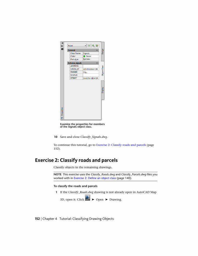
Examine the properties for membersof the Signals object class.
10 Save and close Classify_Signals.dwg.
To continue this tutorial, go to Exercise 2: Classify roads and parcels (page152).
Exercise 2: Classify roads and parcelsClassify objects in the remaining drawings.
NOTE This exercise uses the Classify_Roads.dwg and Classify_Parcels.dwg files youworked with in Exercise 2: Define an object class (page 140).
To classify the roads and parcels
1 If the Classify_Roads.dwg drawing is not already open in AutoCAD Map
3D, open it. Click ➤ Open ➤ Drawing.
152 | Chapter 4 Tutorial: Classifying Drawing Objects
2 Click Create tab ➤ Drawing Object panel ➤ Select Unclassified.
3 Press Enter to select all unclassified objects (page 316).
4 Right-click the Roads object class (page 313) in Map Explorer in the Taskpane and click Classify Objects.
5 Leave both boxes checked in the Classify Objects dialog box and clickOK.
6 Save and close Classify_Roads.dwg.
7 If the Classify_Parcels.dwg drawing is not already open in AutoCAD Map
3D, open it. Click ➤ Open ➤ Drawing.
8 Instead of selecting all the parcels, drag-select only a portion of them.
Select about one quarter of the parcels.
9 Right-click the Parcels object class in Map Explorer in the Task pane andclick Classify Objects.
10 Leave both boxes checked in the Classify Objects dialog box and clickOK.
11 Save and close Classify_Parcels.dwg.
Where you are now
You classified objects for three object classes.
To continue this tutorial, go to Lesson 4: Create a Map Using Object Classes(page 153).
Lesson 4: Create a Map Using Object ClassesNow that you saved the object class definitions in a file, you can attach thatfile to any map to use the definitions. You can also attach the drawings whoseobjects are classified, and query those objects into the map with the definitionfile attached to it. The combination of the definition file and the classifiedobjects in the attached drawings determines that AutoCAD Map 3D treats theobjects as classified.
Lesson 4: Create a Map Using Object Classes | 153
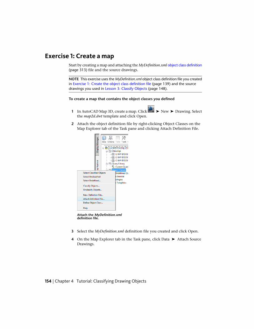
Exercise 1: Create a mapStart by creating a map and attaching the MyDefinition.xml object class definition(page 313) file and the source drawings.
NOTE This exercise uses the MyDefinition.xml object class definition file you createdin Exercise 1: Create the object class definition file (page 139) and the sourcedrawings you used in Lesson 3: Classify Objects (page 148).
To create a map that contains the object classes you defined
1 In AutoCAD Map 3D, create a map. Click ➤ New ➤ Drawing. Selectthe map2d.dwt template and click Open.
2 Attach the object definition file by right-clicking Object Classes on theMap Explorer tab of the Task pane and clicking Attach Definition File.
Attach the MyDefinition.xmldefinition file.
3 Select the MyDefinition.xml definition file you created and click Open.
4 On the Map Explorer tab in the Task pane, click Data ➤ Attach SourceDrawings.
154 | Chapter 4 Tutorial: Classifying Drawing Objects
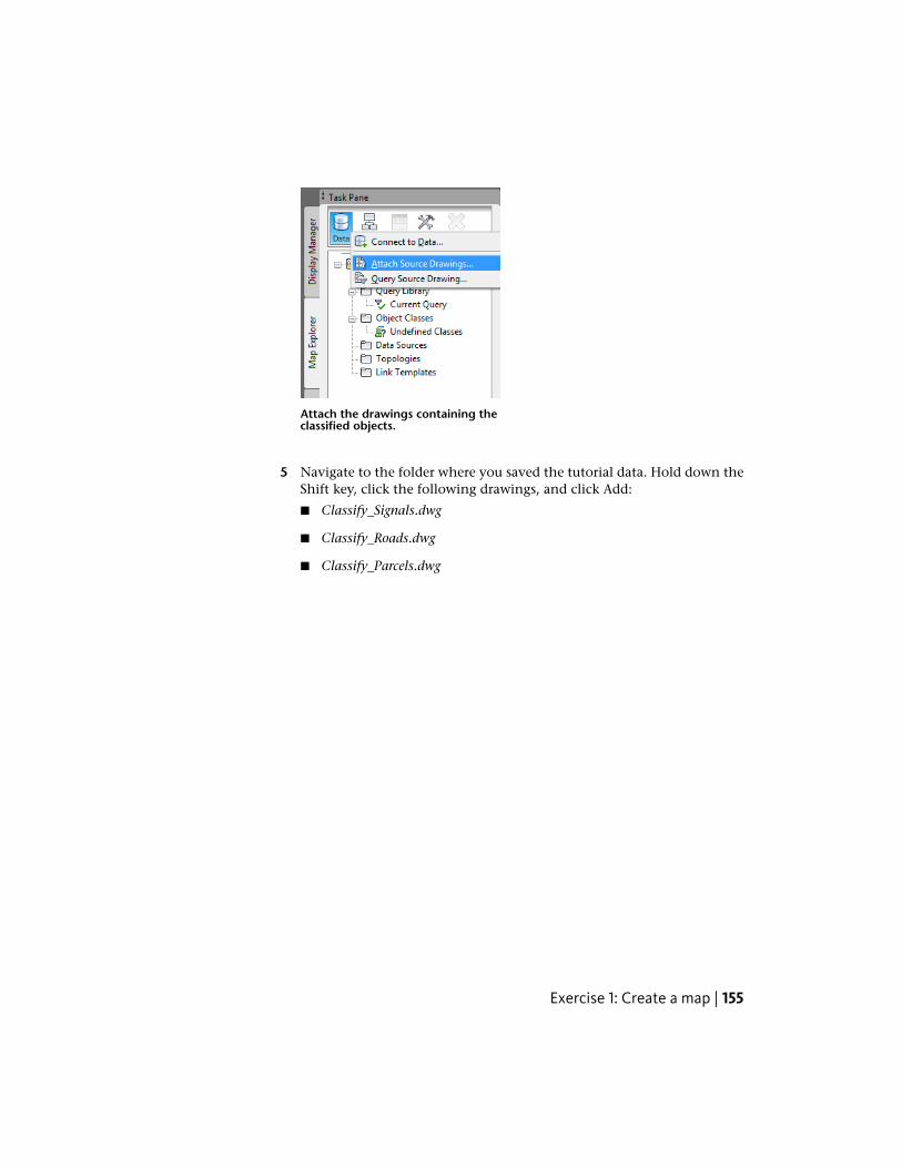
Attach the drawings containing theclassified objects.
5 Navigate to the folder where you saved the tutorial data. Hold down theShift key, click the following drawings, and click Add:
■ Classify_Signals.dwg
■ Classify_Roads.dwg
■ Classify_Parcels.dwg
Exercise 1: Create a map | 155

Select all three drawing files.
6 Click OK.
NOTE You might see an alert as you work through the remainder of thetutorial. The alert warns that the association between queried objects in thecurrent and attached drawings is not retained once the current drawing fileis closed. This message reminds you to save back any changes you make tothe original drawing file. You can safely ignore the alert.
To continue this tutorial, go to Exercise 2: Assign a coordinate system (page156).
Exercise 2: Assign a coordinate systemAssign a coordinate system to the current map and the attached drawings atone time.
156 | Chapter 4 Tutorial: Classifying Drawing Objects

NOTE This exercise uses the map you created in Exercise 1: Create a map (page154).
To assign a coordinate system to the current map and to the attacheddrawings
1 Click Map Setup tab ➤ Coordinate System panel ➤ Assign.
Assign a coordinate system to the current and attacheddrawings.
2 Under Current Drawing, for Code, type CA-I (uppercase C, uppercase A,hyphen, uppercase I). Press Enter. The dialog box displays the descriptionof this coordinate system.
3 Under Source Drawings, click Select Drawings and select all three attacheddrawings. Click Add and then click OK.
4 Under Source Drawings, for Code, type CA-I and press Enter (as in step2).
5 Click OK.
To continue this tutorial, go to Exercise 3: Query in objects (page 158).
Exercise 2: Assign a coordinate system | 157
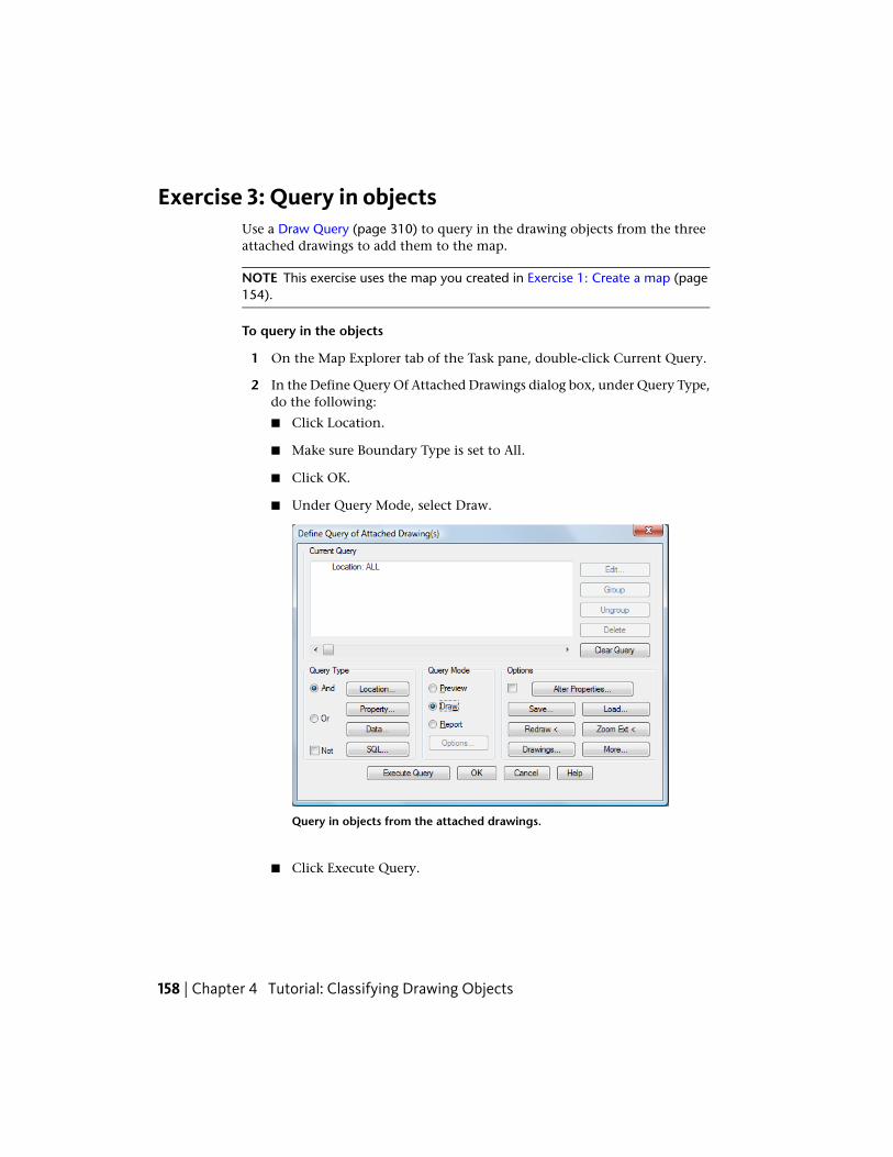
Exercise 3: Query in objectsUse a Draw Query (page 310) to query in the drawing objects from the threeattached drawings to add them to the map.
NOTE This exercise uses the map you created in Exercise 1: Create a map (page154).
To query in the objects
1 On the Map Explorer tab of the Task pane, double-click Current Query.
2 In the Define Query Of Attached Drawings dialog box, under Query Type,do the following:
■ Click Location.
■ Make sure Boundary Type is set to All.
■ Click OK.
■ Under Query Mode, select Draw.
Query in objects from the attached drawings.
■ Click Execute Query.
158 | Chapter 4 Tutorial: Classifying Drawing Objects
3 Click View tab ➤ Navigate panel ➤ Zoom drop-down ➤ Extents. The map is centered on the data.
4 Name and save the map.
■ Click ➤ Save.
■ Navigate to the folder where your tutorial data is stored.
■ Name the map file ObjectClass.dwg.
■ Click Save.
Where you are now
You created a new map that uses the object class definition (page 313) file youdefined. You queried in objects to the new map.
To continue this tutorial, go to Lesson 5: Create and Edit Objects Using ObjectClasses (page 159).
Lesson 5: Create and Edit Objects Using ObjectClasses
You can use object class definitions as a shortcut when you create or changeclassified objects. In this lesson, you create and edit objects using object classes.
Exercise 1: Create objects using object classesWhen you create a new object using object classification, the new objectinherits the basic properties for its object class (page 313) with default valuesfor those properties. You can change the values as needed.
When you query in objects from a DWG file to a map, any styling informationis lost. Since the points are not styled, you cannot see them in your new map.To see the signal points, assign a point style to your map.
Once the signals are visible, you create a signal using the Signals object class.
NOTE This exercise uses the map you created in Exercise 1: Create objects usingobject classes (page 159).
Lesson 5: Create and Edit Objects Using Object Classes | 159

To assign a point style to your map
1 If the ObjectClass.dwg file you created in the previous exercise is not still
open, open it. Click ➤ Open ➤ Drawing.
2 To assign a point style, at the command prompt enter ddptype.
3 In the Point Style dialog box, select any point style in the second row.You can use the default point size settings.
Select a point style for the signals.
4 Click OK.
To create a Signals object
1 Zoom in until you can see the signal points easily.
2 On the Map Explorer tab of the Task pane, right-click the Signals objectclass and click Create Classified Object.
160 | Chapter 4 Tutorial: Classifying Drawing Objects
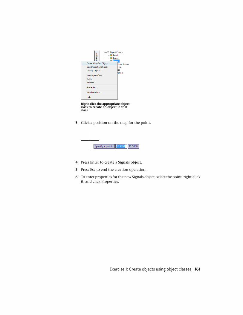
Right-click the appropriate objectclass to create an object in thatclass.
3 Click a position on the map for the point.
4 Press Enter to create a Signals object.
5 Press Esc to end the creation operation.
6 To enter properties for the new Signals object, select the point, right-clickit, and click Properties.
Exercise 1: Create objects using object classes | 161
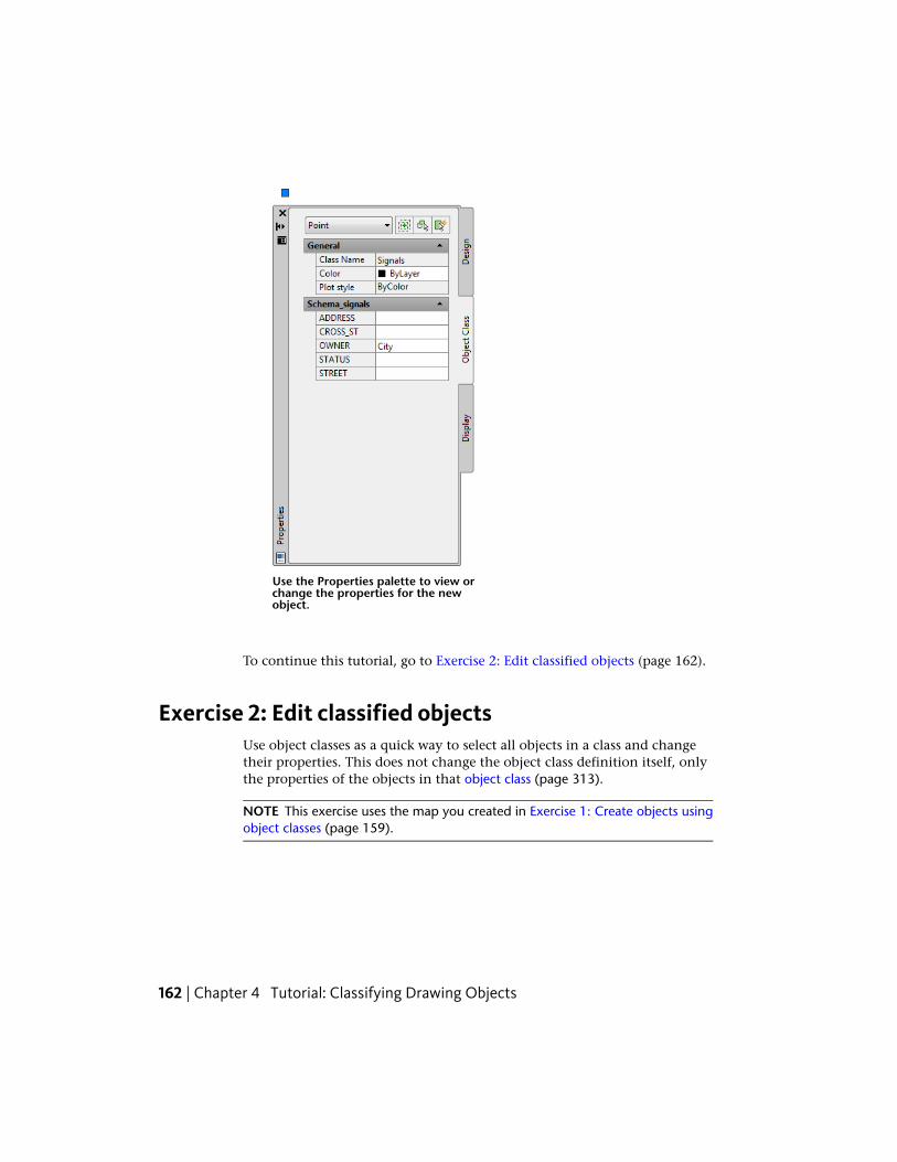
Use the Properties palette to view orchange the properties for the newobject.
To continue this tutorial, go to Exercise 2: Edit classified objects (page 162).
Exercise 2: Edit classified objectsUse object classes as a quick way to select all objects in a class and changetheir properties. This does not change the object class definition itself, onlythe properties of the objects in that object class (page 313).
NOTE This exercise uses the map you created in Exercise 1: Create objects usingobject classes (page 159).
162 | Chapter 4 Tutorial: Classifying Drawing Objects

To change the color of the classified parcels
1 If the ObjectClass.dwg file you created previously is not still open, open
it. Click ➤ Open ➤ Drawing.
2 On the Map Explorer tab of the Task pane, right-click the Parcels objectclass name.
3 Click Select Classified Objects.
All objects classified as Parcels are selected.
4 Right-click any of the selected parcels and click Properties.
5 In the Properties palette, click the Pattern Fill Color field (under Patternon the Design tab) and choose a different color.
Exercise 2: Edit classified objects | 163
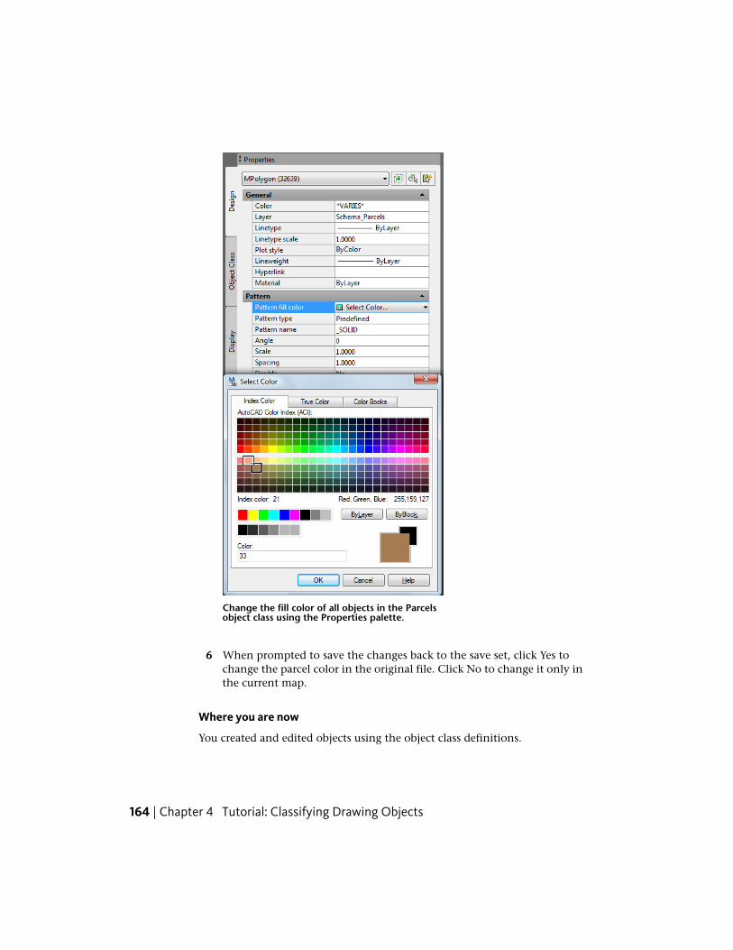
Change the fill color of all objects in the Parcelsobject class using the Properties palette.
6 When prompted to save the changes back to the save set, click Yes tochange the parcel color in the original file. Click No to change it only inthe current map.
Where you are now
You created and edited objects using the object class definitions.
164 | Chapter 4 Tutorial: Classifying Drawing Objects
To continue this tutorial, go to Lesson 6: Generate Metadata for a ClassifiedDrawing (page 165).
Lesson 6: Generate Metadata for a ClassifiedDrawing
Metadata is data about data. For example, metadata includes informationabout object class definitions, as well as more general information, such asthe coordinate system used by the drawing. When you classify objects in adrawing, AutoCAD Map 3D generates metadata automatically. You can viewand share this metadata.
Exercise 1: View metadataWhen you open the Metadata Viewer for the first time, metadata (page 313) isautomatically generated and displayed for the current drawing if the drawingcontains classified objects.
The metadata is stored inside the drawing itself. Metadata is updated eachtime you edit the drawing or reconnect to the attached drawings that containclassified objects.
NOTE This exercise uses the map you created in Exercise 1: Create objects usingobject classes (page 159).
To view metadata
1 If the ObjectClass.dwg file you created previously is not still open, open
it. Click ➤ Open ➤ Drawing.
2 Click the Map Explorer tab on the Task pane.
3 Expand the Object Classes item.
4 Right-click an object class (page 313) and click View Metadata.
5 In the Metadata Viewer, scroll down to see the various fields and data.
Lesson 6: Generate Metadata for a Classified Drawing | 165

Metadata for classified drawings is generated automatically.
To continue this tutorial, go to Exercise 2: Share metadata (page 166).
Exercise 2: Share metadataYou can export metadata (page 313) from your drawing to an XML file withthe extension .mtd. A linking file is also created and placed in the same locationas the MTD file. You can set an Auto Update option in the Metadata Optionsdialog box. With this option on, the linking file remembers the location ofthe data and keeps the exported metadata current.
NOTE This exercise uses the map you created in Exercise 1: Create objects usingobject classes (page 159).
To export metadata
1 In the Metadata Viewer, click Options (in the top-right area of theMetadata Viewer window).
166 | Chapter 4 Tutorial: Classifying Drawing Objects

2 In the Metadata Options dialog box, click the Preference tab.
3 Select the Auto Update When Selecting Data Source option.
4 Click OK.
5 In the Metadata Viewer, click Export (at the top of the Metadata Viewerwindow).
6 In the Export Metadata dialog box, do the following:
■ Select All Items In and select the Object Classes check box.
■ For Location, click Browse and navigate to a folder for the exportedmetadata and link files.For example, navigate to the folder where you copied your tutorialfiles.
■ Click Export.
Use object classes to organize the exported metadata.
Where you are now
You generated metadata (page 313) that included object class (page 313)information. You exported the metadata for the object classes.
To continue this tutorial, go to Lesson 7: Use Object Classes When Exporting(page 168).
Exercise 2: Share metadata | 167

Lesson 7: Use Object Classes When ExportingWhen you export to a spatial data format, such as Autodesk SDF, Oracle, orSHP, you create feature classes. Feature classes are like object classes: they haveproperties that represent the geometry of objects, as well as properties thatrepresent attribute data. Some database spatial data formats support multiplefeature classes within a single file. These formats include Oracle, SQL Server,and some file-based data formats, such as Autodesk SDF. Some formats (forexample, SHP) store only a single feature class in each file.
If you have classified objects in your drawing, you can use the object classesas the basis for the new feature classes. In this lesson, you export the objectclasses in your drawing to multiple feature classes in a single Autodesk SDFfile. You then connect to that file in a new drawing to see how the resultingfeature classes appear in a map.
Exercise 1: Export object classes to SDFIn this exercise, you export the object classes in your drawing to multiplefeature classes in a single Autodesk SDF file.
NOTE This exercise uses the map you created in Exercise 1: Create objects usingobject classes (page 159).
To export to an Autodesk SDF file using object classes
1 If the ObjectClass.dwg file you created previously is not still open, openit.
2 Click Output tab ➤ Map Data Transfer panel ➤ As SDF.
3 In the Export Location dialog box, do the following:
■ Make sure that Files Of Type is set to Autodesk SDF (*.sdf).
■ Navigate to the folder where you copied the tutorial data.
■ For the file name, enter Roads_Parcels_Signals.sdf.
■ Click OK.
4 In the Export dialog box, under Filter Selection, click Select Object Classes.
168 | Chapter 4 Tutorial: Classifying Drawing Objects

5 In the Select Object Classes dialog box, hold down the Ctrl or Shift keyand click all three object classes. Click Select.
6 In the Export dialog box, click the Feature Class tab and do the following:
■ Under Object To Feature Class Mapping, click Create Multiple ClassesBased On Drawing Object.
■ For Drawing Object To Use, select Object Class.
■ Click Select Attributes.
7 In the Select Attributes dialog box, expand the Object Classes item andselect all three object classes. Click OK.
The new SDF file will contain one feature class for each object class (page313) you selected. The properties of each feature class match the attributesof its corresponding object class.
8 On the Feature Class tab of the Export dialog box, under Object To FeatureClass Mapping, specify the appropriate Geometry entry:
■ For Roads, select Line.
■ For Parcels, select Polygon.
■ For Signals, select Point.
Exercise 1: Export object classes to SDF | 169
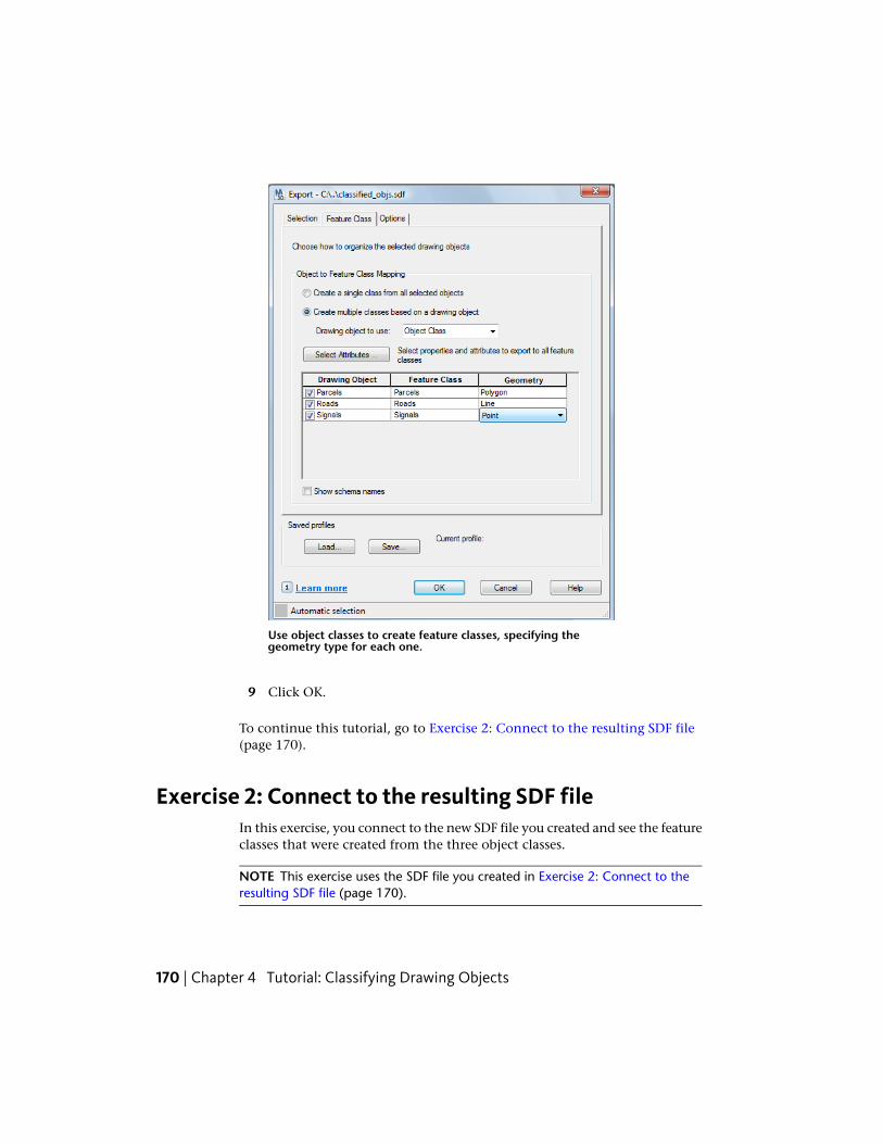
Use object classes to create feature classes, specifying thegeometry type for each one.
9 Click OK.
To continue this tutorial, go to Exercise 2: Connect to the resulting SDF file(page 170).
Exercise 2: Connect to the resulting SDF fileIn this exercise, you connect to the new SDF file you created and see the featureclasses that were created from the three object classes.
NOTE This exercise uses the SDF file you created in Exercise 2: Connect to theresulting SDF file (page 170).
170 | Chapter 4 Tutorial: Classifying Drawing Objects
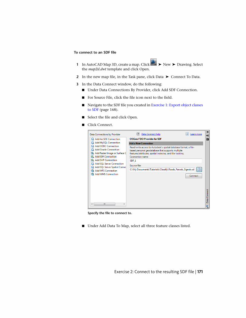
To connect to an SDF file
1 In AutoCAD Map 3D, create a map. Click ➤ New ➤ Drawing. Selectthe map2d.dwt template and click Open.
2 In the new map file, in the Task pane, click Data ➤ Connect To Data.
3 In the Data Connect window, do the following:
■ Under Data Connections By Provider, click Add SDF Connection.
■ For Source File, click the file icon next to the field.
■ Navigate to the SDF file you created in Exercise 1: Export object classesto SDF (page 168).
■ Select the file and click Open.
■ Click Connect.
Specify the file to connect to.
■ Under Add Data To Map, select all three feature classes listed.
Exercise 2: Connect to the resulting SDF file | 171
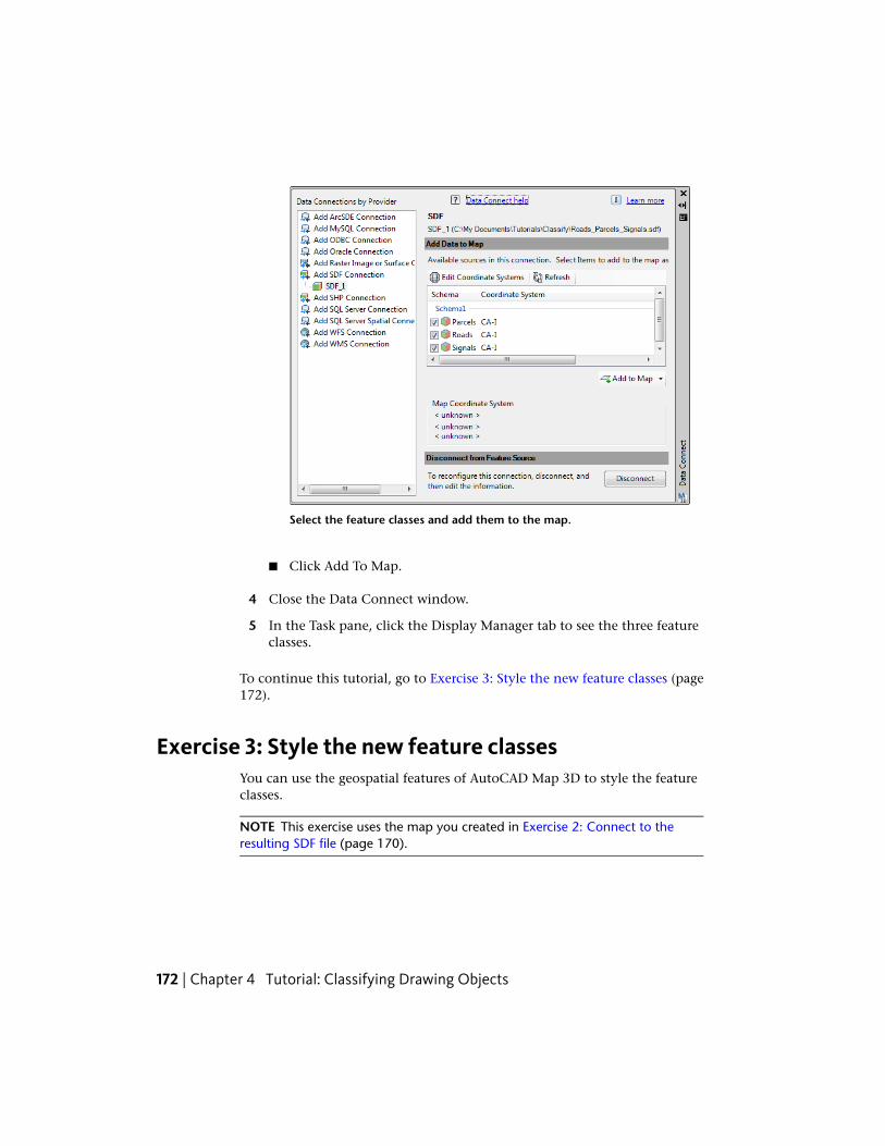
Select the feature classes and add them to the map.
■ Click Add To Map.
4 Close the Data Connect window.
5 In the Task pane, click the Display Manager tab to see the three featureclasses.
To continue this tutorial, go to Exercise 3: Style the new feature classes (page172).
Exercise 3: Style the new feature classesYou can use the geospatial features of AutoCAD Map 3D to style the featureclasses.
NOTE This exercise uses the map you created in Exercise 2: Connect to theresulting SDF file (page 170).
172 | Chapter 4 Tutorial: Classifying Drawing Objects

To style the feature classes
1 If the map you created in the previous exercise is not still open, reopenit.
2 In Display Manager, click the Parcels layer and click Style.
3 In the Style Editor, click in the Style field.
4 In the Style Polygon dialog box, change the Foreground Color to a lightbrown and click OK.
5 With the Style Editor still open, click the Roads layer in Display Manager.
6 In the Style Editor, do the following:
■ Click the browse button next to the Feature Label field.
■ In the Style Label dialog box, from the Property To Display list, selectST_NAME. Click OK.
■ In the Style Editor, click in the Style field.
■ In the Style Line dialog box, change the Color to a dark gray.
7 With the Style Editor still open, click the Signals layer in Display Manager.
8 In the Style Editor, click in the Style field.
9 In the Style Point dialog box, do the following:
■ Click the browse button next to Symbol and choose the round symbol.
■ Change the Fill Color and Edge Color to a light gray.
10 Close the Style Editor.
The map is now styled with the colors and symbols you chose. The roads arelabeled with their street names. The original data is unaffected by these stylingchanges.
Where you are now
You used object classes to export the drawing objects to a geospatial format.
To learn about guidelines to follow when using object classification, go toObject Classification: Best Practices (page 174).
Exercise 3: Style the new feature classes | 173

Object Classification: Best PracticesWhen setting up and using object classification, follow these guidelines forthe best results:
■ Use only one object class definition (page 313) file for a project. Object classesshould be general enough that a definition for “roads” is appropriate inany circumstance. Create subclasses for freeways, parkways, small streets,and so on.
■ Only one person should edit object class definitions at a time, or one setof edits might be lost. If the definition file was just edited, quit AutoCADMap 3D and restart it to get the updated definitions.
■ Distinguish between the Object Type (on the Applies To tab of the DefineObject Classification dialog box) and the Create Method (on the ClassSettings tab). Object Type determines which existing objects you can addto this object class (page 313). If the object was not created with the selectedmethod, you cannot add it. Create Method determines the method usedto create new objects from this class (when you right-click the object classand choose Create Classified Object).
NOTE If you plan to use this object class with objects from a drawing source,do not select more than one object type
■ Avoid renaming object classes, because this changes the name only in theobject class definition file. Objects tagged with the object class name areunchanged. Since these objects point to a name that no longer exists inthe object class definition file, the objects become undefined. You cansearch for undefined objects and update their object class name.
■ Avoid including styling options in object class definitions. For example,you can draw points using a block. You can specify that block if you useBlock as the Create Method for an object class that represents point data.However, the block will not scale to the map, and might cause more workthan it saves. Instead, create a drawing layer in Display Manager and assignthe point objects to that layer. Style the layer from Display Manager usingthe desired block.
174 | Chapter 4 Tutorial: Classifying Drawing Objects

Tutorial: Creating a MapBook With an Inset
About the Map Book TutorialA map book is like an atlas: it takes a single map and divides it into "tiles" byplacing a grid over it. Each square of the grid becomes a map tile. Each tile isthen rendered on a separate page, which you can publish to a plotter or to anelectronic format called DWF. Once you publish a map to DWF, you can shareit with people who do not have a copy of AutoCAD Map 3D. These people candownload Autodesk Design Review (page 309), a free viewer available fromhttp://www.autodesk.com, to see the maps.
Map books use viewports to organize the information on each page. A viewportis like a frame on a web page. You can create a custom viewport as an inset (page312) on one or more of the map book pages. Pan and zoom within that viewportto display an enlarged detail of the map.
You can also link a regular “key” viewport on the map book to a copy of themain map file. Then, every tile of the map book displays the overall map in asmall window.
Lesson 1: Prepare the MapIn this lesson, you create a map and add the city boundary and roads for thecity of Redding, California.
5
175
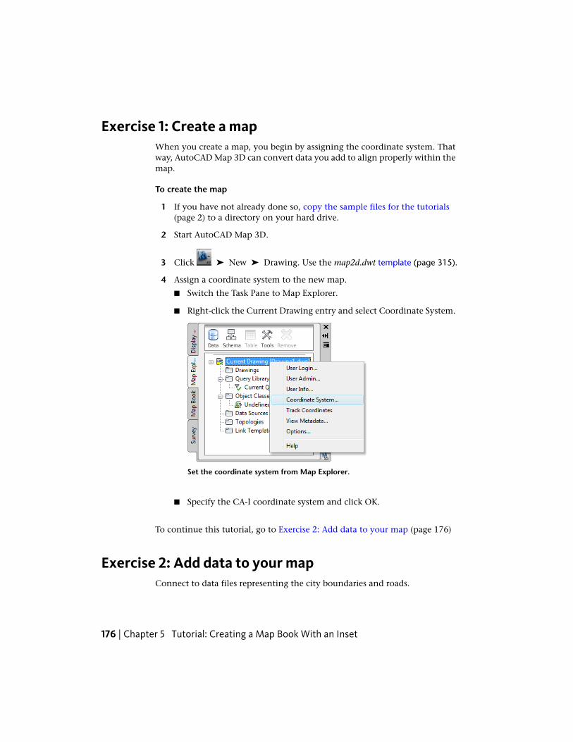
Exercise 1: Create a mapWhen you create a map, you begin by assigning the coordinate system. Thatway, AutoCAD Map 3D can convert data you add to align properly within themap.
To create the map
1 If you have not already done so, copy the sample files for the tutorials(page 2) to a directory on your hard drive.
2 Start AutoCAD Map 3D.
3 Click ➤ New ➤ Drawing. Use the map2d.dwt template (page 315).
4 Assign a coordinate system to the new map.
■ Switch the Task Pane to Map Explorer.
■ Right-click the Current Drawing entry and select Coordinate System.
Set the coordinate system from Map Explorer.
■ Specify the CA-I coordinate system and click OK.
To continue this tutorial, go to Exercise 2: Add data to your map (page 176)
Exercise 2: Add data to your mapConnect to data files representing the city boundaries and roads.
176 | Chapter 5 Tutorial: Creating a Map Book With an Inset
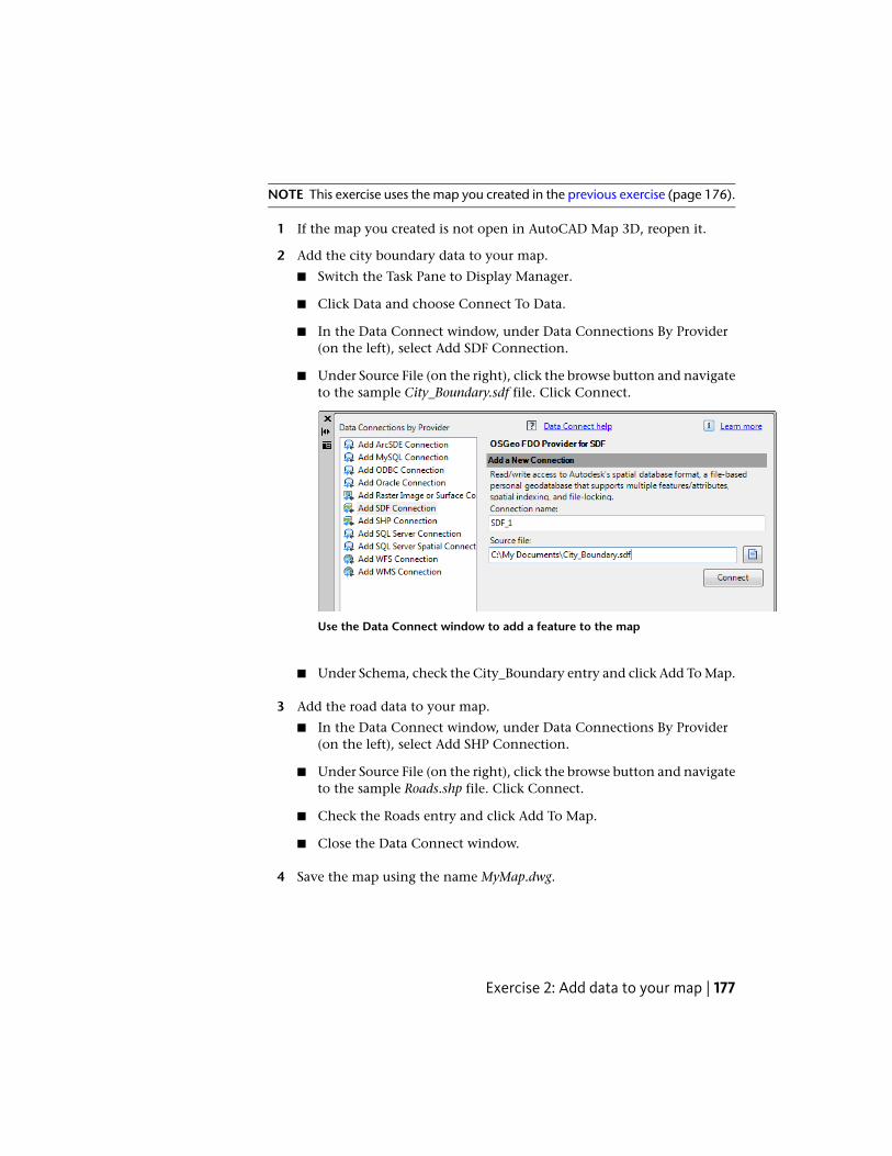
NOTE This exercise uses the map you created in the previous exercise (page 176).
1 If the map you created is not open in AutoCAD Map 3D, reopen it.
2 Add the city boundary data to your map.
■ Switch the Task Pane to Display Manager.
■ Click Data and choose Connect To Data.
■ In the Data Connect window, under Data Connections By Provider(on the left), select Add SDF Connection.
■ Under Source File (on the right), click the browse button and navigateto the sample City_Boundary.sdf file. Click Connect.
Use the Data Connect window to add a feature to the map
■ Under Schema, check the City_Boundary entry and click Add To Map.
3 Add the road data to your map.
■ In the Data Connect window, under Data Connections By Provider(on the left), select Add SHP Connection.
■ Under Source File (on the right), click the browse button and navigateto the sample Roads.shp file. Click Connect.
■ Check the Roads entry and click Add To Map.
■ Close the Data Connect window.
4 Save the map using the name MyMap.dwg.
Exercise 2: Add data to your map | 177

Where you are now
You created a map and connected to feature sources for the city boundariesand the roads of Redding, California.
To continue this tutorial, go to Lesson 2: Customize a Map Book Template(page 178)
Lesson 2: Customize a Map Book TemplateAutoCAD Map 3D comes with a variety of map book templates that make iteasy to create a map book. Each template (page 315) contains all the basic mapbook elements, which you can customize for a particular purpose.
Exercise 1: Change the printer/plotter for the templateOpen an existing map book template (page 315) and begin customizing it byspecifying your printer or plotter.
NOTE This information is used every time you publish your map book to a plotter.You cannot change these settings at print time.
To assign a printer or plotter to a map book template
1 Open the 8.5x11 map book template.
■ Click ➤ Open ➤ Drawing.
■ Change Files Of Type to Drawing Template (*.DWT).AutoCAD Map 3D automatically changes to the Template folder.
■ Scroll about halfway down the list of templates.
■ Select Map Book Template - 8.5x11 Classic.dwt.
■ Click Open.
178 | Chapter 5 Tutorial: Creating a Map Book With an Inset
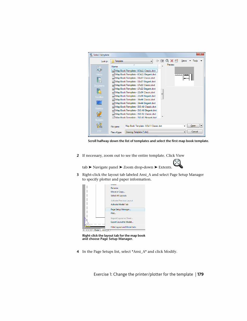
Scroll halfway down the list of templates and select the first map book template.
2 If necessary, zoom out to see the entire template. Click View
tab ➤ Navigate panel ➤ Zoom drop-down ➤ Extents.
3 Right-click the layout tab labeled Ansi_A and select Page Setup Managerto specify plotter and paper information.
Right-click the layout tab for the map bookand choose Page Setup Manager.
4 In the Page Setups list, select *Ansi_A* and click Modify.
Exercise 1: Change the printer/plotter for the template | 179
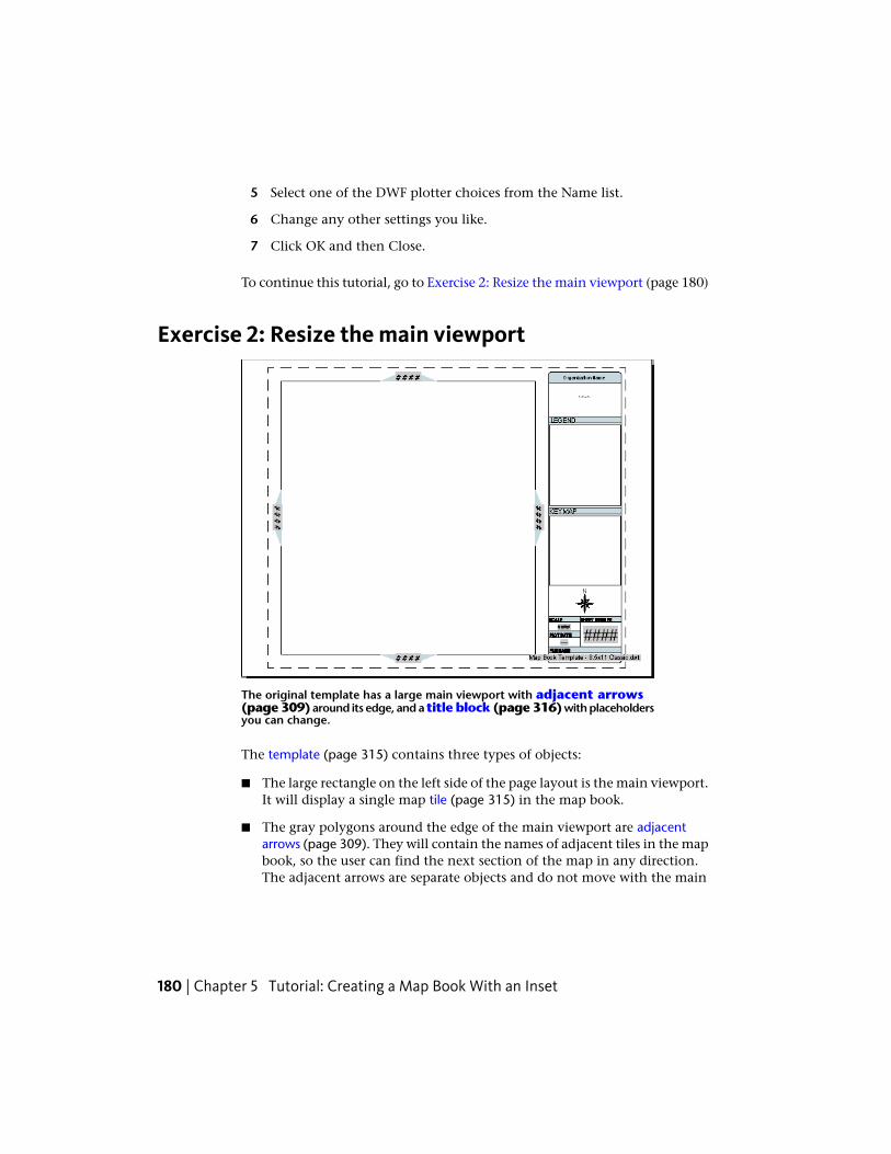
5 Select one of the DWF plotter choices from the Name list.
6 Change any other settings you like.
7 Click OK and then Close.
To continue this tutorial, go to Exercise 2: Resize the main viewport (page 180)
Exercise 2: Resize the main viewport
The original template has a large main viewport with adjacent arrows(page 309) around its edge, and a title block (page 316) with placeholdersyou can change.
The template (page 315) contains three types of objects:
■ The large rectangle on the left side of the page layout is the main viewport.It will display a single map tile (page 315) in the map book.
■ The gray polygons around the edge of the main viewport are adjacentarrows (page 309). They will contain the names of adjacent tiles in the mapbook, so the user can find the next section of the map in any direction.The adjacent arrows are separate objects and do not move with the main
180 | Chapter 5 Tutorial: Creating a Map Book With an Inset
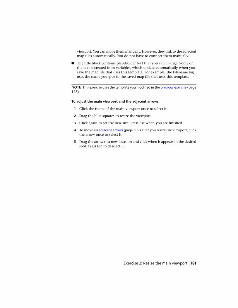
viewport. You can move them manually. However, they link to the adjacentmap tiles automatically. You do not have to connect them manually.
■ The title block contains placeholder text that you can change. Some ofthe text is created from variables, which update automatically when yousave the map file that uses this template. For example, the Filename taguses the name you give to the saved map file that uses this template.
NOTE This exercise uses the template you modified in the previous exercise (page178).
To adjust the main viewport and the adjacent arrows
1 Click the frame of the main viewport once to select it.
2 Drag the blue squares to resize the viewport.
3 Click again to set the new size. Press Esc when you are finished.
4 To move an adjacent arrows (page 309) after you resize the viewport, clickthe arrow once to select it.
5 Drag the arrow to a new location and click when it appears in the desiredspot. Press Esc to deselect it.
Exercise 2: Resize the main viewport | 181
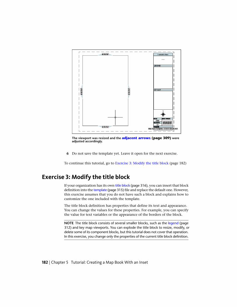
The viewport was resized and the adjacent arrows (page 309) wereadjusted accordingly.
6 Do not save the template yet. Leave it open for the next exercise.
To continue this tutorial, go to Exercise 3: Modify the title block (page 182)
Exercise 3: Modify the title blockIf your organization has its own title block (page 316), you can insert that blockdefinition into the template (page 315) file and replace the default one. However,this exercise assumes that you do not have such a block and explains how tocustomize the one included with the template.
The title block definition has properties that define its text and appearance.You can change the values for these properties. For example, you can specifythe value for text variables or the appearance of the borders of the block.
NOTE The title block consists of several smaller blocks, such as the legend (page312) and key map viewports. You can explode the title block to resize, modify, ordelete some of its component blocks, but this tutorial does not cover that operation.In this exercise, you change only the properties of the current title block definition.
182 | Chapter 5 Tutorial: Creating a Map Book With an Inset
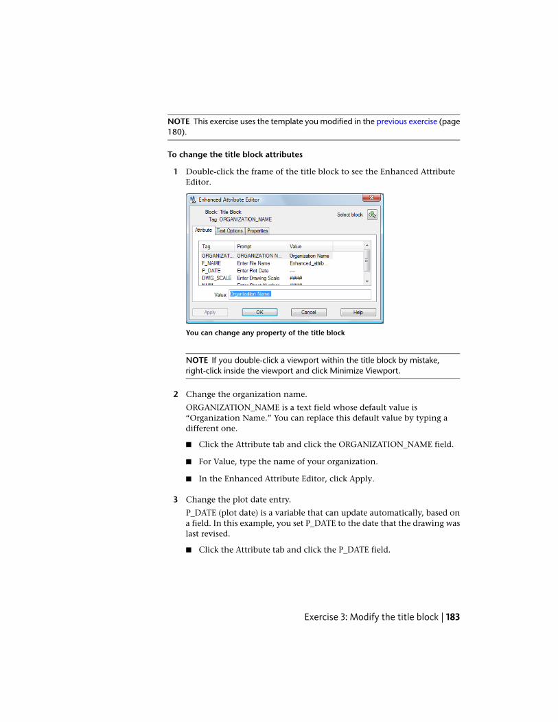
NOTE This exercise uses the template you modified in the previous exercise (page180).
To change the title block attributes
1 Double-click the frame of the title block to see the Enhanced AttributeEditor.
You can change any property of the title block
NOTE If you double-click a viewport within the title block by mistake,right-click inside the viewport and click Minimize Viewport.
2 Change the organization name.
ORGANIZATION_NAME is a text field whose default value is“Organization Name.” You can replace this default value by typing adifferent one.
■ Click the Attribute tab and click the ORGANIZATION_NAME field.
■ For Value, type the name of your organization.
■ In the Enhanced Attribute Editor, click Apply.
3 Change the plot date entry.
P_DATE (plot date) is a variable that can update automatically, based ona field. In this example, you set P_DATE to the date that the drawing waslast revised.
■ Click the Attribute tab and click the P_DATE field.
Exercise 3: Modify the title block | 183
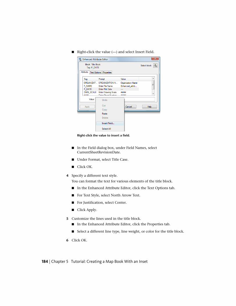
■ Right-click the value (---) and select Insert Field.
Right-click the value to insert a field.
■ In the Field dialog box, under Field Names, selectCurrentSheetRevisionDate.
■ Under Format, select Title Case.
■ Click OK.
4 Specify a different text style.
You can format the text for various elements of the title block.
■ In the Enhanced Attribute Editor, click the Text Options tab.
■ For Text Style, select North Arrow Text.
■ For Justification, select Center.
■ Click Apply.
5 Customize the lines used in the title block.
■ In the Enhanced Attribute Editor, click the Properties tab.
■ Select a different line type, line weight, or color for the title block.
6 Click OK.
184 | Chapter 5 Tutorial: Creating a Map Book With an Inset

7 Save the modified template.
■ Click ➤ Save As ➤ AutoCAD Drawing Template.
■ Specify a new name (for example, Map Book Template - Inset.dwt).Save the template in the Templates directory if you plan to reuse it.Otherwise, save it in My Documents.
8 Edit the description when it displays. Leave Save All Layers AsUnreconciled selected.
9 Leave the template file open for the next exercise.
To continue this tutorial, go to Exercise 4: Replace the north arrow block (page185).
Exercise 4: Replace the north arrow blockAutoCAD Map 3D comes with sample files, including blocks such as northarrow symbols. You can delete the default north arrow and replace it withone of the sample blocks.
The template (page 315) also has an area in which you can insert your companylogo as a block. The process would be similar.
NOTE This exercise uses the template you modified in the previous exercise (page182).
To replace the north arrow in the map book template
1 If the template you modified is not still open, open it again.
2 Click the north arrow block in the template and press Delete.
3 Open the sample file containing the north arrow symbols.
By default, the north arrow file is C:\Program Files\AutoCAD Map 3D2010\Sample\Symbols\North Arrows.dwg.
4 In the North Arrows.dwg file, click a north arrow symbol.
5 Right-click the selected symbol and click Copy.
6 Close the North Arrows.dwg file and, in the template file, right-click ablank area and click Paste As Block.
Exercise 4: Replace the north arrow block | 185

7 At the Specify Insertion Point prompt, click the location for the newnorth arrow.
8 Save and close the template file.
Where you are now
You modified a map book template to use your printer or plotter. You changedthe size of the main viewport and adjusted the adjacent arrows (page 309). Youchanged the attributes of the title block (page 316). You replaced the defaultnorth arrow with another one.
To continue this tutorial, go to Lesson 3: Create A Map Book (page 186)
Lesson 3: Create A Map BookYou create a map book within the map file itself—not within the template(page 315). When you create the map book, you specify the template to use.In this case, you specify the template you modified in Lesson 2 (page 178) (MapBook Template - Inset.dwt).
Exercise 1: Create a key map view and a legendThe template (page 315) contains a viewport called a key map. The key mapview displays the same content for every tile (page 315) in the map book. Often,a key view (page 312) contains the entire mapped area, to provide context forthe smaller area represented by the tile.
You can link the key map viewport to any external drawing. In this exercise,you save a copy of the current drawing to use as a key map view.
The template also contains a viewport called Legend. You can link this viewportto an external drawing you use as a legend (page 312), or (if your map containsa legend), to the internal legend. In this exercise, you generate a legend forthe map to display in the Legend viewport.
1 Open the map you created in Lesson 1: Prepare the Map (page 175).
For example, if you named the map from lesson 1 MyMap.dwg, open thatfile.
2 Create a copy of the map to use as a key map view. Click ➤ SaveAs ➤ AutoCAD Drawing.
186 | Chapter 5 Tutorial: Creating a Map Book With an Inset

Save the map with a similar name to the original one. For example, if theoriginal map is MyMap.dwg, save this version as MyMapKeyView.dwg.
3 Close the map file and reopen the original one (MyMap.dwg).
You will use MyMapKeyView.dwg in the next exercise, when you link itto the Key Map viewport.
4 Generate a legend that you can link to the Legend viewport.
■ Switch the Task Pane to the Display Manager tab.
■ Click Tools ➤ Create Legend.
■ Click a blank space that is outside the bounding box of the mappedarea.Make sure there is some space between the map itself and the legend.That way, you can define the tiled area for the map book withoutincluding the legend in it.
To continue this tutorial, go to Exercise 2: Specify the map book settings (page187).
Exercise 2: Specify the map book settingsThe Create Map Book dialog box guides you through all the settings neededfor a map book. You can save your settings to use for future map books.
NOTE This exercise uses the map you modified in the previous exercise (page186).
To specify the map book settings
1 On the Display Manager tab of the Task Pane, right-click theCity_Boundary layer and click Zoom To Extents.
2 Save the map file.
You cannot publish a map to any format without saving it first.
3 Switch the Task Pane to Map Book and click New ➤ Map Book.
Exercise 2: Specify the map book settings | 187

Each item on the left displays settings on the right.
4 In the Create Map Book dialog box, for Source, click Model Space.Optionally, change the Map Book Name.
5 For Sheet Template, do the following:
■ Click Settings.
■ Click the browse button for Choose A Sheet Template and navigateto the saved template (page 315) you created (Map Book Template -Inset.dwt).
■ Leave the layout set to Ansi_A.
■ For Layout Options, check Include A Title Block (Name Or File) andInclude Adjacent Sheet Links (Name Or File).
■ For the title block (page 316), click the down arrow and click Title Block.For adjacent sheet links, click the down arrow and clickAdjacent_Arrow_4.
188 | Chapter 5 Tutorial: Creating a Map Book With an Inset
■ Set the scale factor to 50000.
NOTE If you don't set the Scale Factor, the map book will comprise avery large number of tiles (page 315). Be sure to set it to 50000.
6 For Tiling Scheme, do the following:
■ Click By Area.
■ Click Select Area To Tile and drag a rectangle around the extents ofthe map.
■ Leave the other settings set to their defaults.
7 For Naming Scheme, click Columns And Rows. Leave the settings set totheir defaults.
8 For Key, click External Reference. Browse to the key view (page 312) mapyou created in the previous exercise (page 186) and select it.
The Key Map viewport will display the key map you generated in theprevious exercise.
9 For Legend, click Map Display.
The Legend viewport will display the legend (page 312) you generated inthe previous exercise (page 186).
10 For Sheet Set, click Create New.
Do not generate the map yet. Leave the dialog box open for the nextexercise.
To continue this tutorial, go on to Exercise 3: Preview and generate the mapbook (page 189).
Exercise 3: Preview and generate the map bookYou can see how the map book will be divided into tiles (page 315) before yougenerate it.
NOTE This exercise uses the map you modified in the previous exercise (page187).
Exercise 3: Preview and generate the map book | 189
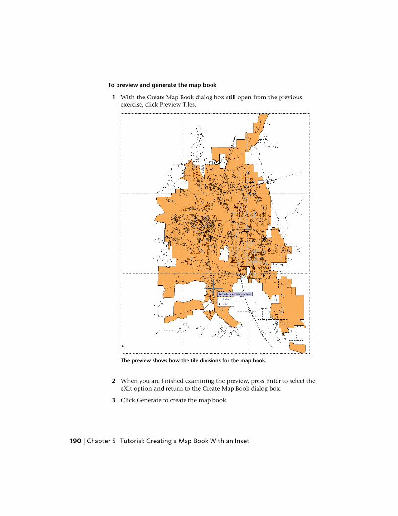
To preview and generate the map book
1 With the Create Map Book dialog box still open from the previousexercise, click Preview Tiles.
The preview shows how the tile divisions for the map book.
2 When you are finished examining the preview, press Enter to select theeXit option and return to the Create Map Book dialog box.
3 Click Generate to create the map book.
190 | Chapter 5 Tutorial: Creating a Map Book With an Inset

When you generate the map book, the tiles are listed in the Task Pane,and one layout tab is displayed for each tile.
Each letter represents a row oftiles, with the numbered tiles forthat row indented below it
One layout tab is created for each of the map book tiles
4 Click one of the new layout tabs to see the portion of the map that itcontains.
Exercise 3: Preview and generate the map book | 191
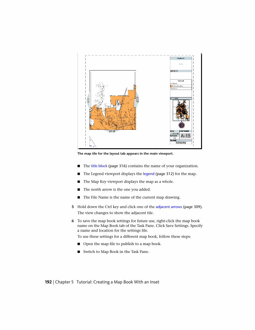
The map tile for the layout tab appears in the main viewport.
■ The title block (page 316) contains the name of your organization.
■ The Legend viewport displays the legend (page 312) for the map.
■ The Map Key viewport displays the map as a whole.
■ The north arrow is the one you added.
■ The File Name is the name of the current map drawing.
5 Hold down the Ctrl key and click one of the adjacent arrows (page 309).
The view changes to show the adjacent tile.
6 To save the map book settings for future use, right-click the map bookname on the Map Book tab of the Task Pane. Click Save Settings. Specifya name and location for the settings file.
To use these settings for a different map book, follow these steps:
■ Open the map file to publish to a map book.
■ Switch to Map Book in the Task Pane.
192 | Chapter 5 Tutorial: Creating a Map Book With an Inset
■ Click New ➤ Map Book From Settings.
■ Select the settings file you saved.
Where you are now
You previewed and generated the map book, producing multiple tiles thateach contain a portion of the original map. You used the layout tabs to viewindividual tiles, and the adjacent arrows (page 309) to move between tiles.
To continue this tutorial, go to Lesson 4: Create an Inset (page 193)
Lesson 4: Create an InsetYou will create an inset (page 312) on one tile (page 315) in the map book. Theinset is a new viewport that you set up to display a particular area and zoomlevel.
Exercise 1: Draw a viewport for the insetYou can create your own viewports, as well as customizing the ones that appearon the template (page 315) by default. In this exercise, you will draw a viewporton a map tile (page 315) to show a zoomed-in detail.
NOTE This exercise uses the map you modified in the previous lesson (page 186).
To create the viewport
1 Click the layout tab for the tile on which the inset (page 312) will appear.
In this example, the inset appears on B-25.
2 At the Command prompt, type vports.
The Command prompt appears as soon as you begin typing anywherewithin the map window.
3 On the New Viewports tab of the Viewports dialog box, in the StandardViewports list, select Single and click OK.
4 Place your cursor over the blank area next to the main viewport.
5 Drag to draw the viewport on the layout, and click when it is the sizeyou want.
Lesson 4: Create an Inset | 193

6 Leave the map open and the current layout tab displayed for the followingexercise.
To continue this tutorial, go to Exercise 2: Change the information displayedin the viewport (page 194)
Exercise 2: Change the information displayed in theviewport
When you first create the viewport, it displays the entire map. You can zoomin to display a detail for this map tile (page 315) instead.
NOTE This exercise uses the map you modified in the previous exercise (page193).
1 The layout tab with the new viewport you created in the previous exercise(page 193) should still be displayed. If not, reopen it.
2 Double-click inside the new viewport.
3 Use any AutoCAD Map 3D zoom and pan commands to display the areaof interest for this map tile.
194 | Chapter 5 Tutorial: Creating a Map Book With an Inset
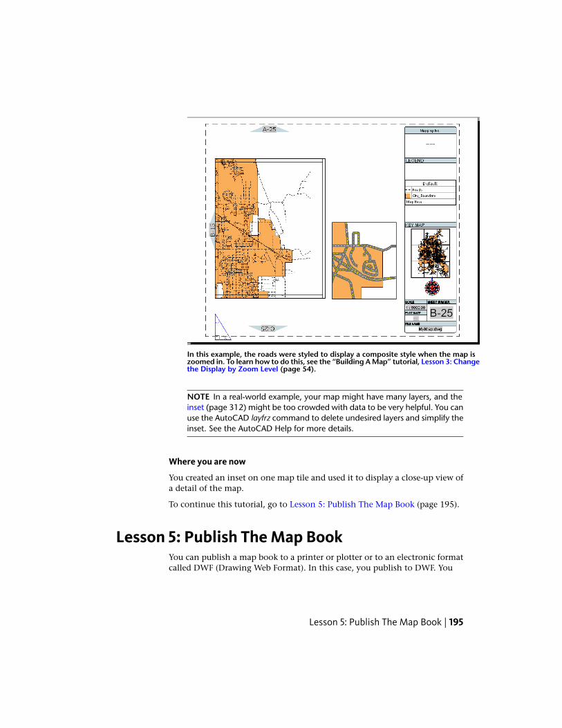
In this example, the roads were styled to display a composite style when the map iszoomed in. To learn how to do this, see the “Building A Map” tutorial, Lesson 3: Changethe Display by Zoom Level (page 54).
NOTE In a real-world example, your map might have many layers, and theinset (page 312) might be too crowded with data to be very helpful. You canuse the AutoCAD layfrz command to delete undesired layers and simplify theinset. See the AutoCAD Help for more details.
Where you are now
You created an inset on one map tile and used it to display a close-up view ofa detail of the map.
To continue this tutorial, go to Lesson 5: Publish The Map Book (page 195).
Lesson 5: Publish The Map BookYou can publish a map book to a printer or plotter or to an electronic formatcalled DWF (Drawing Web Format). In this case, you publish to DWF. You
Lesson 5: Publish The Map Book | 195
can share a DWF file with people who do not have a copy of AutoCAD Map3D. These people can download a free viewer, Autodesk Design Review (page309), from http://www.autodesk.com/designreview to view the DWF file.
Exercise 1: Set DWF publishing optionsSet the options that control the information published with the map.
NOTE This exercise uses the map you modified in the previous lesson (page 193).
To set DWF options
1 If you closed the map file from the previous exercise (page 194), reopenit.
2 Click Output tab ➤ Export To DWF/PDF panel ➤ DWF Options.
3 Select the Publish Map Information check box.
4 Expand the GIS Feature Sources item to see what is included.
If you expand the list all the way, you can see the properties associatedwith the features in this map.
5 Check the GIS Feature Sources item.
All subitems are automatically checked.
196 | Chapter 5 Tutorial: Creating a Map Book With an Inset

The Map Information dialog boxdetermines which data is published to DWF
Optionally, you can select just a subset of the properties.
6 Click OK.
The first time you set these options, specify a name and location for thepublishing settings. In subsequent publishing sessions, AutoCAD Map3D uses the last settings file you used.
To continue this tutorial, go to Exercise 2: Set background publishing options(page 197).
Exercise 2: Set background publishing optionsPublishing is faster if you turn off background publishing. Settings you changein this dialog box remain in effect for all new drawings until you change thesettings again.
NOTE This exercise uses the map you modified in the previous exercise (page196).
To set background publishing options
1 Click ➤ Options.
Exercise 2: Set background publishing options | 197
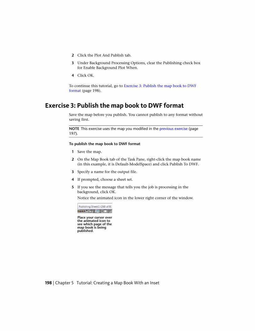
2 Click the Plot And Publish tab.
3 Under Background Processing Options, clear the Publishing check boxfor Enable Background Plot When.
4 Click OK.
To continue this tutorial, go to Exercise 3: Publish the map book to DWFformat (page 198).
Exercise 3: Publish the map book to DWF formatSave the map before you publish. You cannot publish to any format withoutsaving first.
NOTE This exercise uses the map you modified in the previous exercise (page197).
To publish the map book to DWF format
1 Save the map.
2 On the Map Book tab of the Task Pane, right-click the map book name(in this example, it is Default-ModelSpace) and click Publish To DWF.
3 Specify a name for the output file.
4 If prompted, choose a sheet set.
5 If you see the message that tells you the job is processing in thebackground, click OK.
Notice the animated icon in the lower right corner of the window.
Place your cursor overthe animated icon tosee which page of themap book is beingpublished.
198 | Chapter 5 Tutorial: Creating a Map Book With an Inset
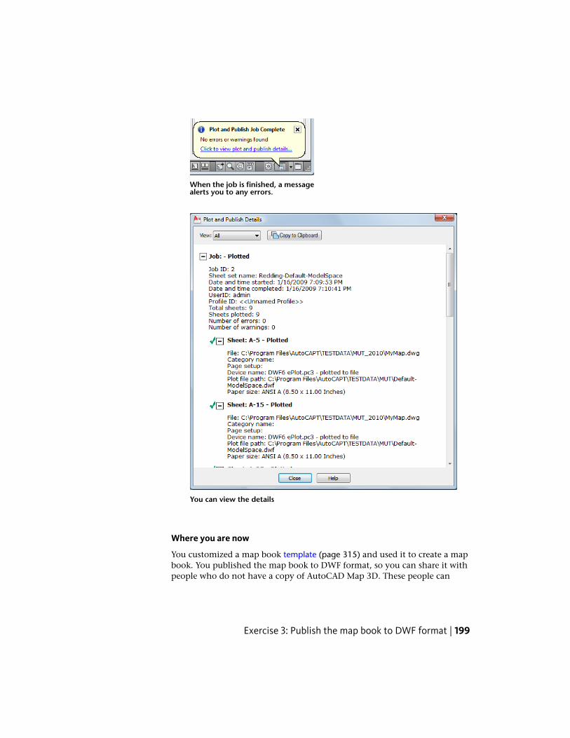
When the job is finished, a messagealerts you to any errors.
You can view the details
Where you are now
You customized a map book template (page 315) and used it to create a mapbook. You published the map book to DWF format, so you can share it withpeople who do not have a copy of AutoCAD Map 3D. These people can
Exercise 3: Publish the map book to DWF format | 199

download a free viewer, Autodesk Design Review (page 309), to see the maps.Autodesk Design Review is available from http://www.autodesk.com/designreview.
200 | Chapter 5 Tutorial: Creating a Map Book With an Inset

Tutorial: Analyzing Data
About the Analyzing Data TutorialThis tutorial demonstrates the following ways to analyze data in AutoCAD Map3D:
■ Analyze data visually, using surfaces.Connect to a surface (DEM) image and style it using a theme to show relativeelevation. Then, connect to a file that shows parcel information and makethe parcels semi-transparent so you can see the raster image below them.The elevation theme of the raster helps you see the elevation of the parcels.
■ Analyze data with external information using joins.Join a Microsoft Access database to a parcels layer to see information aboutthe parcel owners. Joins combine data sources temporarily, without alteringthe original data stores. Use the combined data as though it were a singledata source. For example, style a layer based on its joined data, even thoughthe joined data is not part of the original layer data store. Create calculatedfields using native and joined data.
■ Analyze data by proximity using buffers.Define a buffer around a street to see which parcels lie within a constructionzone. Select the parcels that adjoin the buffer and save them separately soyou can notify their owners, using the owner information you joined to theparcels.
Export relevant data to a comma-separated file that you can import intoMicrosoft Excel or Access. Use that data to create a report to send to theowners.
■ Perform a flood analysis with Overlay.
6
201
Overlay a flood zone layer with a layer representing the business zone.Add a roads layer to see which streets in the business zone lie within theflood zone. Add a layer representing hospitals to see which areas are thefurthest from help if the area floods.
■ Automate an overlay operation with a workflow.Edit a workflow that performs an overlay operation. Set the parameters tothe ones used in the overlay tutorial to automate the overlay.
Lesson 1: Analyze Data Visually, Using SurfacesUse Data Connect to attach a DEM file to a map. Style the surface to show theelevation information it contains.
Exercise 1: Prepare your map fileCreate a map file and assign a coordinate system. Color the map backgroundwhite so you can better distinguish features when you use color to style them.All maps you create from now on use the new background color.
To create a map file
1 If you have not already done so, copy the sample files for the tutorials(page 2) to a directory on your hard drive.
2 Start AutoCAD Map 3D and create a map using the map2d.dwt template.
3 Assign a coordinate system to the new map.
■ Click Map Setup tab ➤ Coordinate System panel ➤ Assign.
202 | Chapter 6 Tutorial: Analyzing Data
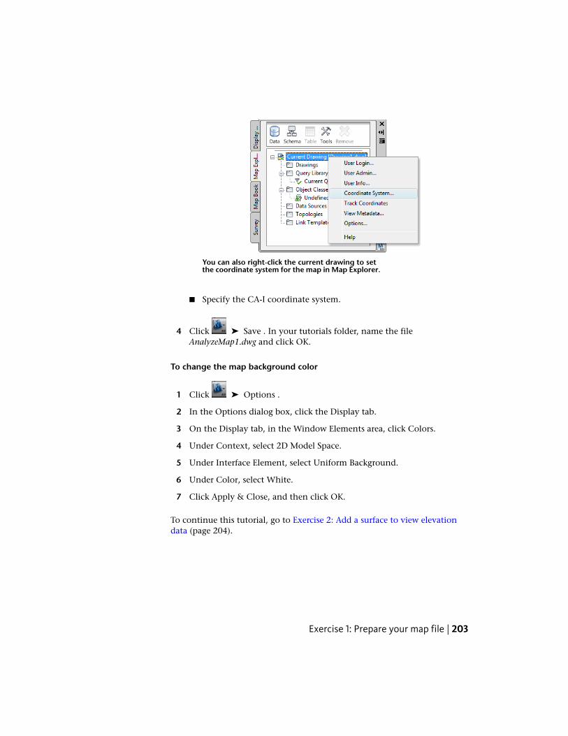
You can also right-click the current drawing to setthe coordinate system for the map in Map Explorer.
■ Specify the CA-I coordinate system.
4 Click ➤ Save . In your tutorials folder, name the fileAnalyzeMap1.dwg and click OK.
To change the map background color
1 Click ➤ Options .
2 In the Options dialog box, click the Display tab.
3 On the Display tab, in the Window Elements area, click Colors.
4 Under Context, select 2D Model Space.
5 Under Interface Element, select Uniform Background.
6 Under Color, select White.
7 Click Apply & Close, and then click OK.
To continue this tutorial, go to Exercise 2: Add a surface to view elevationdata (page 204).
Exercise 1: Prepare your map file | 203

Exercise 2: Add a surface to view elevation dataA surface is a raster file that contains elevation information. Use theming tomake the surface reflect its elevation.
NOTE This exercise uses the AnalyzeMap1.dwg map you created in the previousexercise.
To add a surface to the map
1 Click Home tab ➤ Data panel ➤ Connect.
2 In the Data Connect window, under Data Connections By Provider, click
Add Raster Image Or Surface Connection and click next to SourceFile Or Folder.
3 In the Open dialog box, browse to the ENTERPRISE.dem file, select it, andclick Open.
Look for this file where you copied the sample data.
Connect to the surface file in the Data Connect window.
4 In the Data Connect window, click Connect.
204 | Chapter 6 Tutorial: Analyzing Data
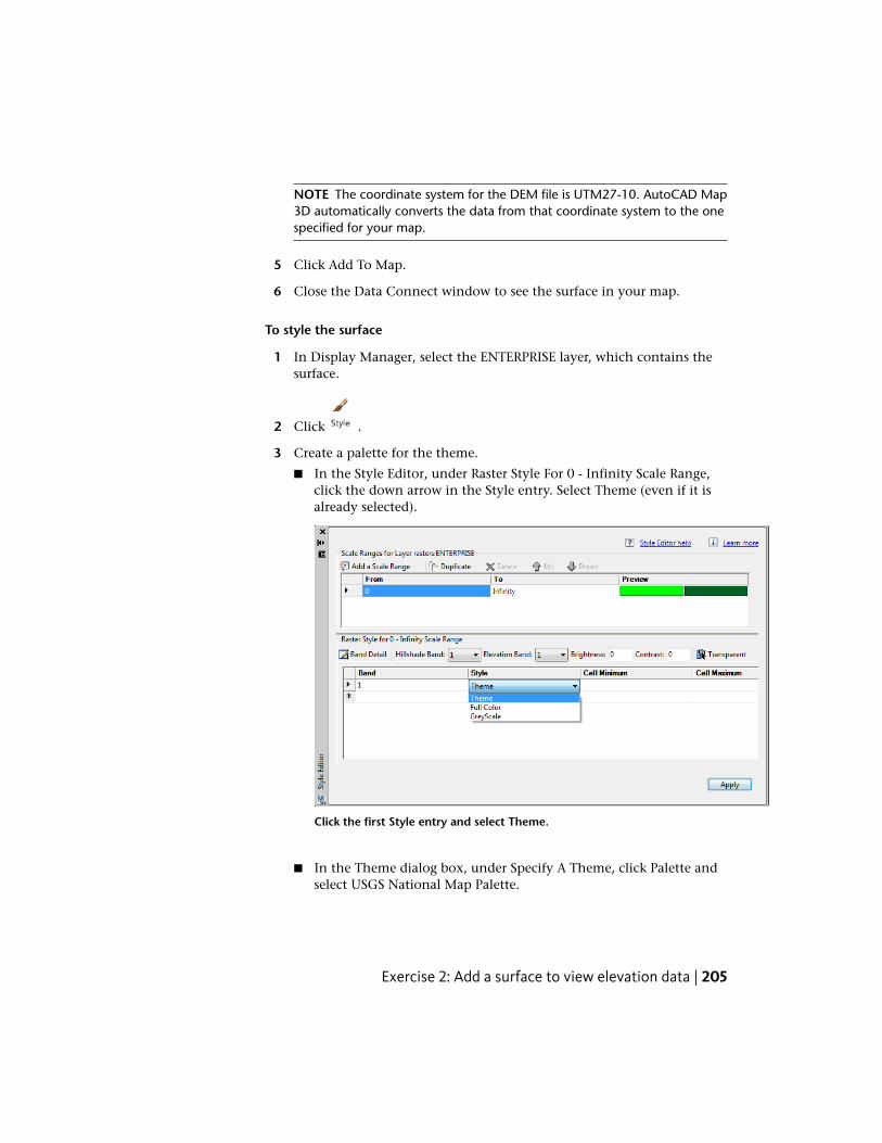
NOTE The coordinate system for the DEM file is UTM27-10. AutoCAD Map3D automatically converts the data from that coordinate system to the onespecified for your map.
5 Click Add To Map.
6 Close the Data Connect window to see the surface in your map.
To style the surface
1 In Display Manager, select the ENTERPRISE layer, which contains thesurface.
2 Click .
3 Create a palette for the theme.
■ In the Style Editor, under Raster Style For 0 - Infinity Scale Range,click the down arrow in the Style entry. Select Theme (even if it isalready selected).
Click the first Style entry and select Theme.
■ In the Theme dialog box, under Specify A Theme, click Palette andselect USGS National Map Palette.
Exercise 2: Add a surface to view elevation data | 205
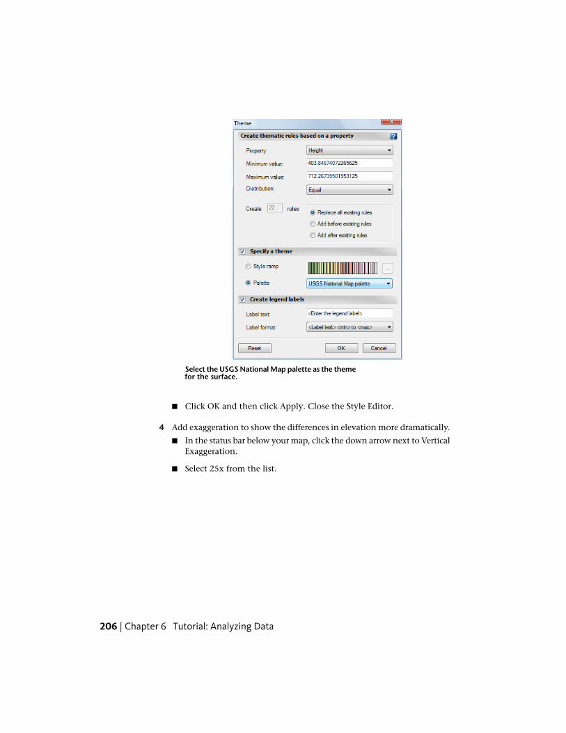
Select the USGS National Map palette as the themefor the surface.
■ Click OK and then click Apply. Close the Style Editor.
4 Add exaggeration to show the differences in elevation more dramatically.
■ In the status bar below your map, click the down arrow next to VerticalExaggeration.
■ Select 25x from the list.
206 | Chapter 6 Tutorial: Analyzing Data
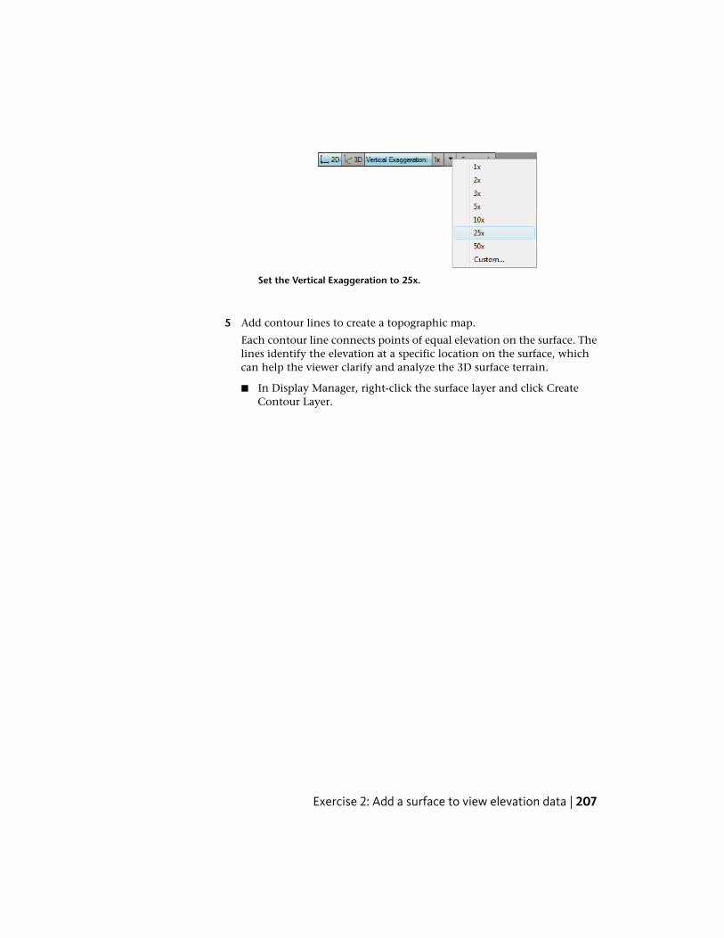
Set the Vertical Exaggeration to 25x.
5 Add contour lines to create a topographic map.
Each contour line connects points of equal elevation on the surface. Thelines identify the elevation at a specific location on the surface, whichcan help the viewer clarify and analyze the 3D surface terrain.
■ In Display Manager, right-click the surface layer and click CreateContour Layer.
Exercise 2: Add a surface to view elevation data | 207
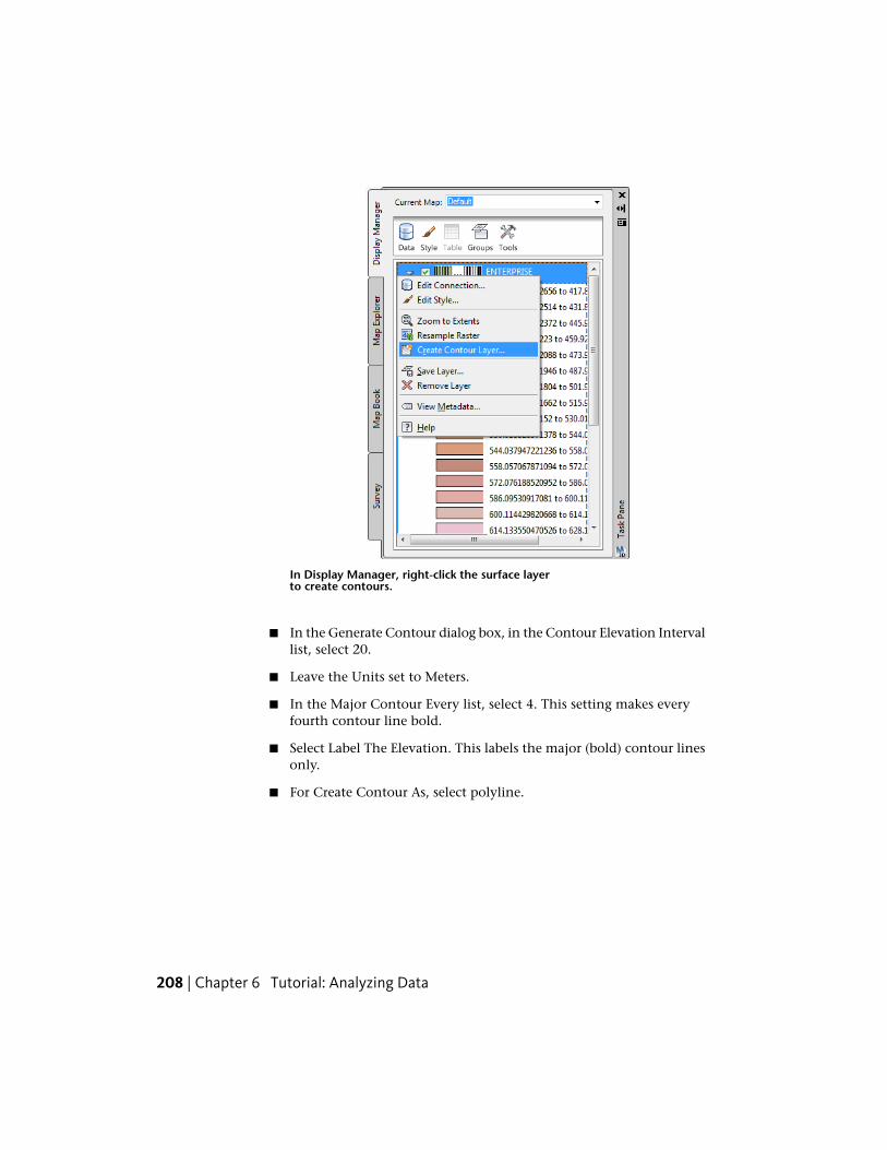
In Display Manager, right-click the surface layerto create contours.
■ In the Generate Contour dialog box, in the Contour Elevation Intervallist, select 20.
■ Leave the Units set to Meters.
■ In the Major Contour Every list, select 4. This setting makes everyfourth contour line bold.
■ Select Label The Elevation. This labels the major (bold) contour linesonly.
■ For Create Contour As, select polyline.
208 | Chapter 6 Tutorial: Analyzing Data

The Generate Contour dialog box settings
■ Click OK.
NOTE To label the intervening contour lines, use the Style Editor to change thestyle for the new contour layer (not the surface layer itself). You can also use thismethod to change the color or style for the contour lines.
■ Select the contour layer in Display Manager and click Style.
■ In the Style Editor, click the down arrow next to the Feature Label entryfor "IsMajor=False."
■ Select Elevation as the Property for the label.
■ Click OK.
To continue this tutorial, go to Exercise 3: Add a layer on top of the surface(page 209).
Exercise 3: Add a layer on top of the surfaceYou can add a vector feature to a map containing a 3D surface. When youdisplay the map in 3D, AutoCAD Map 3D automatically drapes the vector onthe 3D surface.
Exercise 3: Add a layer on top of the surface | 209

NOTE This exercise uses the AnalyzeMap1.dwg map you created and modified inthe previous exercises.
To add roads to the map
1 Click Home tab ➤ Data panel ➤ Connect.
2 In the Data Connect window, under Data Connections By Provider, selectAdd SHP Connection.
3 Click next to the Source File field and navigate to the folder whereyou copied the sample files.
4 In the Open dialog box, select ROADS.SHP and click Open.
5 In the Data Connect window, click Connect.
6 In the Data Connect window, click Add To Map.
7 Close the Data Connect window.
To style the roads in the map
1 In Display Manager, select the Roads layer and click Style.
2 In the Style Editor, click the Style entry.
3 In the Style Line dialog box, change the road color to dark gray.
4 Select a dashed pattern for the lines.
210 | Chapter 6 Tutorial: Analyzing Data
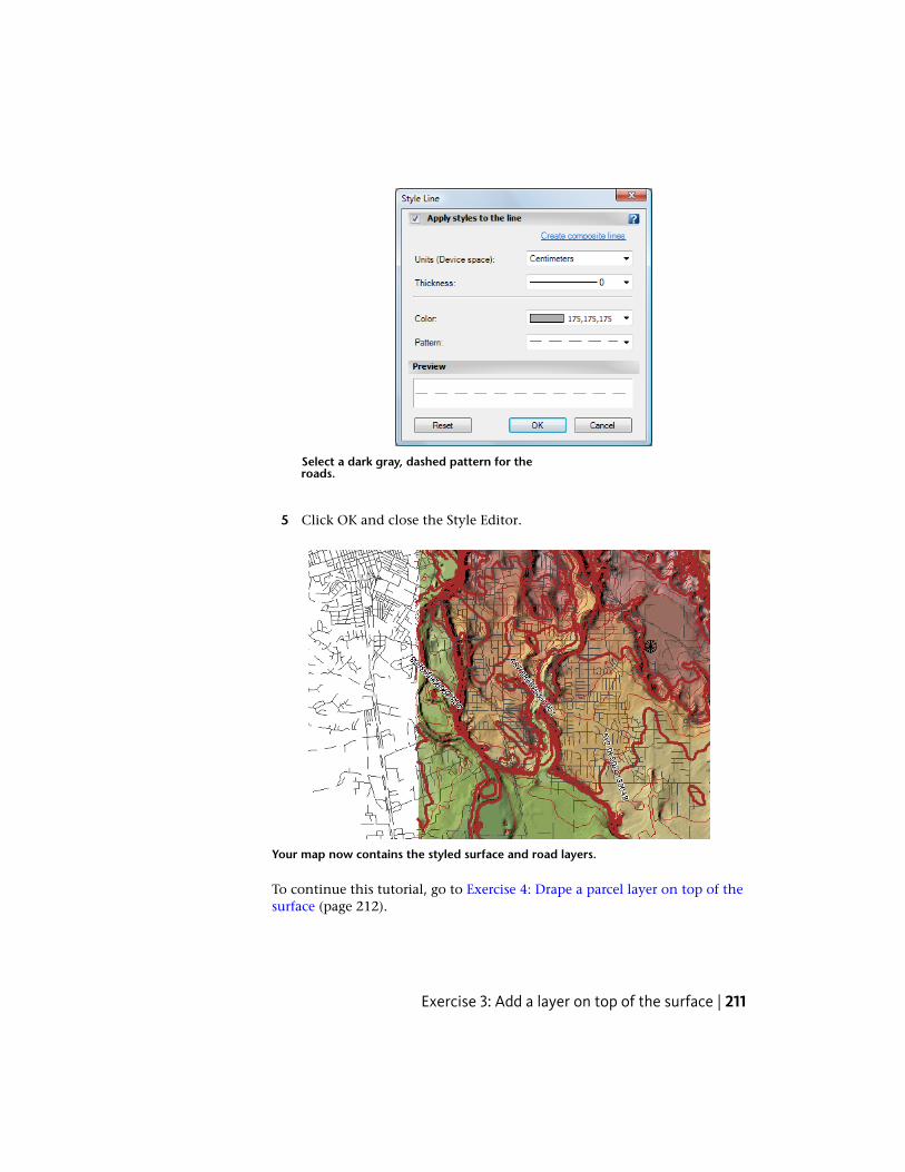
Select a dark gray, dashed pattern for theroads.
5 Click OK and close the Style Editor.
Your map now contains the styled surface and road layers.
To continue this tutorial, go to Exercise 4: Drape a parcel layer on top of thesurface (page 212).
Exercise 3: Add a layer on top of the surface | 211
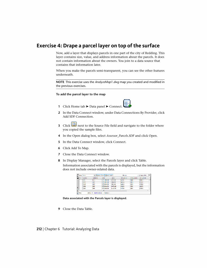
Exercise 4: Drape a parcel layer on top of the surfaceNow, add a layer that displays parcels in one part of the city of Redding. Thislayer contains size, value, and address information about the parcels. It doesnot contain information about the owners. You join to a data source thatcontains that information later.
When you make the parcels semi-transparent, you can see the other featuresunderneath.
NOTE This exercise uses the AnalyzeMap1.dwg map you created and modified inthe previous exercises.
To add the parcel layer to the map
1 Click Home tab ➤ Data panel ➤ Connect.
2 In the Data Connect window, under Data Connections By Provider, clickAdd SDF Connection.
3 Click next to the Source File field and navigate to the folder whereyou copied the sample files.
4 In the Open dialog box, select Assessor_Parcels.SDF and click Open.
5 In the Data Connect window, click Connect.
6 Click Add To Map.
7 Close the Data Connect window.
8 In Display Manager, select the Parcels layer and click Table.
Information associated with the parcels is displayed, but the informationdoes not include owner-related data.
Data associated with the Parcels layer is displayed.
9 Close the Data Table.
212 | Chapter 6 Tutorial: Analyzing Data

To style the parcels in the map
1 In Display Manager, select the Parcels layer and click Style.
2 In the Style Editor, click the color in the Style entry.
3 In the Style Polygon dialog box, change the Foreground Transparencysetting to 50%.
4 Change the Foreground Color to a light shade.
Change the foreground transparency for theparcel layer.
5 Click OK and close the Style Editor.
The parcel layer is draped over the surface. Because it is transparent, youcan see the surface underneath.
Where you are now
You added a surface that contains elevation information, and you used thatinformation to create a theme that varies color by elevation. You added contour
Exercise 4: Drape a parcel layer on top of the surface | 213
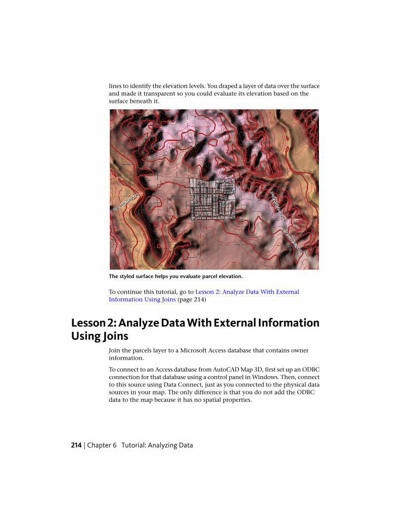
lines to identify the elevation levels. You draped a layer of data over the surfaceand made it transparent so you could evaluate its elevation based on thesurface beneath it.
The styled surface helps you evaluate parcel elevation.
To continue this tutorial, go to Lesson 2: Analyze Data With ExternalInformation Using Joins (page 214)
Lesson 2: Analyze Data With External InformationUsing Joins
Join the parcels layer to a Microsoft Access database that contains ownerinformation.
To connect to an Access database from AutoCAD Map 3D, first set up an ODBCconnection for that database using a control panel in Windows. Then, connectto this source using Data Connect, just as you connected to the physical datasources in your map. The only difference is that you do not add the ODBCdata to the map because it has no spatial properties.
214 | Chapter 6 Tutorial: Analyzing Data

The database source contains a field that you can match to a field in the Parcelslayer. You can join the data to the parcels and style or analyze all the resultingdata seamlessly.
Exercise 1: Set up an ODBC connection for an Accessdatabase
Set up an ODBC connection for the Microsoft Access database using theAdministrative Tools control panel in Windows.
NOTE This exercise uses the AnalyzeMap1.dwg map you created and modified inthe previous exercises.
To set up an ODBC connection for the Access database
1 From your Windows desktop, click Start ➤ Settings ➤ Control Paneland open the Administrative Tools control panel.
2 In the Administrative Tools window, double-click Data Sources (ODBC).
3 In the ODBC Data Source Administrator dialog box, click Add.
4 In the Create New Data Source dialog box, click Microsoft Access Driver(*.mdb) and click Finish.
5 In the ODBC Microsoft Access Setup dialog box, for Data Source Name,enter Parcel_Owners.
6 Enter a description, for example, "Parcel owner information."
Exercise 1: Set up an ODBC connection for an Access database | 215
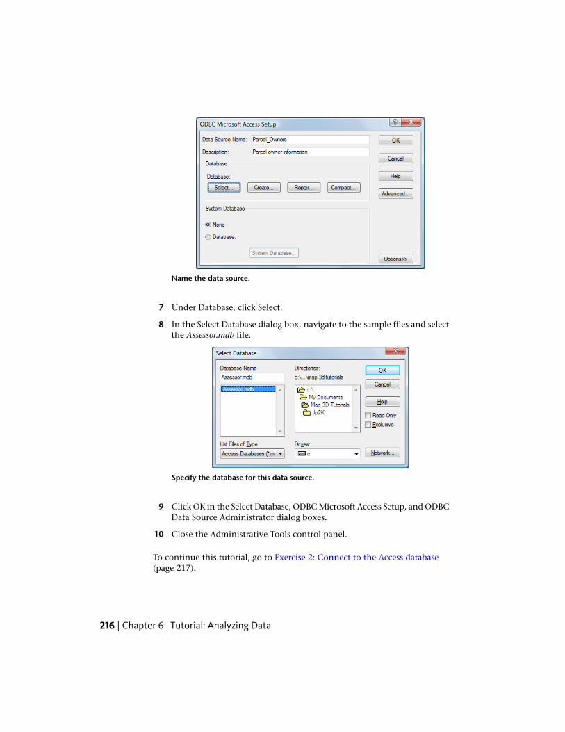
Name the data source.
7 Under Database, click Select.
8 In the Select Database dialog box, navigate to the sample files and selectthe Assessor.mdb file.
Specify the database for this data source.
9 Click OK in the Select Database, ODBC Microsoft Access Setup, and ODBCData Source Administrator dialog boxes.
10 Close the Administrative Tools control panel.
To continue this tutorial, go to Exercise 2: Connect to the Access database(page 217).
216 | Chapter 6 Tutorial: Analyzing Data
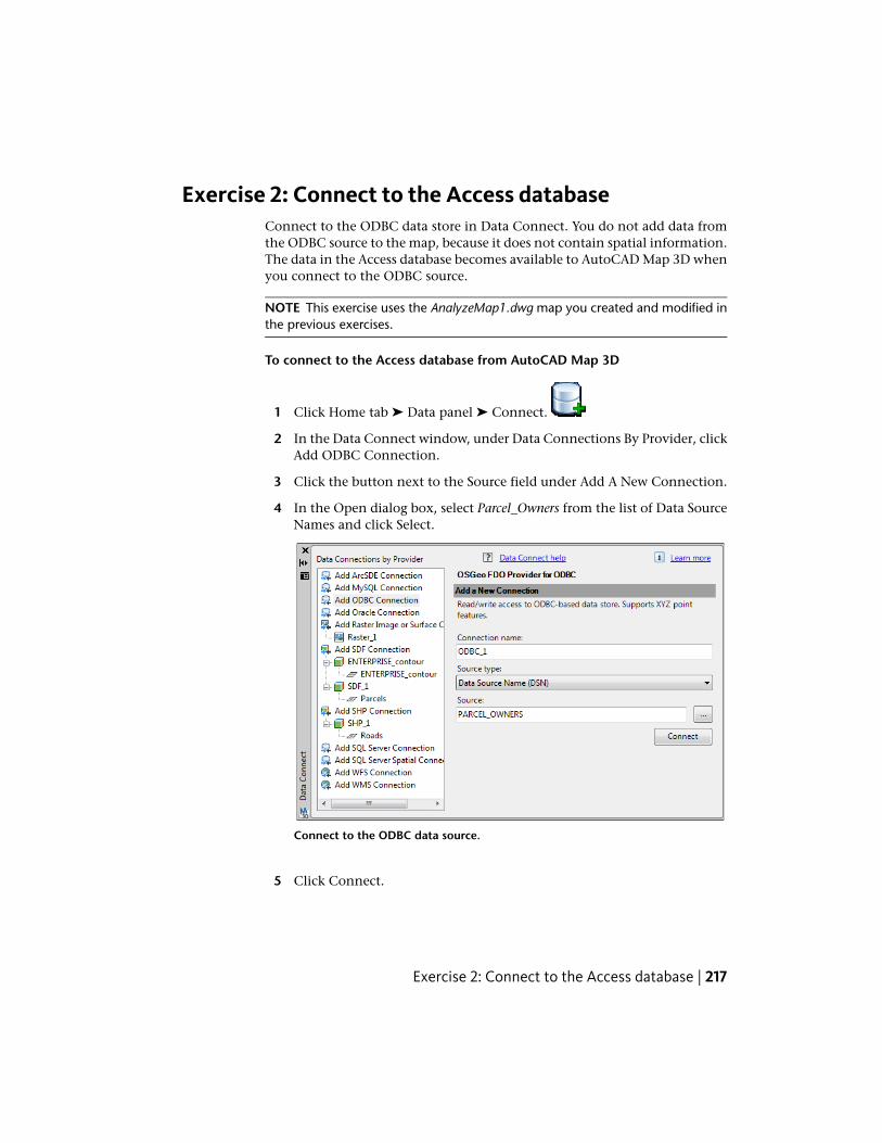
Exercise 2: Connect to the Access databaseConnect to the ODBC data store in Data Connect. You do not add data fromthe ODBC source to the map, because it does not contain spatial information.The data in the Access database becomes available to AutoCAD Map 3D whenyou connect to the ODBC source.
NOTE This exercise uses the AnalyzeMap1.dwg map you created and modified inthe previous exercises.
To connect to the Access database from AutoCAD Map 3D
1 Click Home tab ➤ Data panel ➤ Connect.
2 In the Data Connect window, under Data Connections By Provider, clickAdd ODBC Connection.
3 Click the button next to the Source field under Add A New Connection.
4 In the Open dialog box, select Parcel_Owners from the list of Data SourceNames and click Select.
Connect to the ODBC data source.
5 Click Connect.
Exercise 2: Connect to the Access database | 217
6 In the User Name & Password dialog box, click Login without enteringanything in the fields. (This database has not been set up for user nameand password protection.)
AutoCAD Map 3D has access to the non-spatial data as soon as youconnect to its source.
7 Close the Data Connect window without adding anything to your map.
To continue this tutorial, go to Exercise 3: Join the data from the ODBC sourceto the layer containing the parcels (page 218).
Exercise 3: Join the data from the ODBC source to thelayer containing the parcels
After you connect to an external data source, you can join it to a layer in yourmap using the Data Table. This method works as long as the two data sourcesshare a common property. You can see the results of the join immediately.
NOTE This exercise uses the AnalyzeMap1.dwg map you created and modified inthe previous exercises.
To join the ODBC parcel data to the geospatial parcel layer
1 In Display Manager, select the Parcels layer and click Table.
2 At the bottom of the Data Table, click Options ➤ Create A Join.
In the Create A Join dialog box, the Primary Table Initiating The Joinentry is automatically displayed.
3 For Table (Or Feature Class) To Join To, select the ODBC_1:Fdo:Assessorlayer.
4 For This Column From The Left Table, select APN.
The entry for the corresponding Matches This Column From The RightTable is automatically displayed.
5 Click OK to display all the data in the Data Table.
6 Scroll to the right to see the owner information.
To continue this tutorial, go to Exercise 4: Use the joined data for calculatedfields and styles (page 219).
218 | Chapter 6 Tutorial: Analyzing Data
Exercise 4: Use the joined data for calculated fields andstyles
Now that you have joined owner data to the parcels layer, you can use thejoined information to create a calculated field and determine your styles.
NOTE This exercise uses the AnalyzeMap1.dwg map you created and modified inthe previous exercises.
To create a calculated field using joined data
1 At the bottom of the Data Table, click Options ➤ Create A Calculation.
2 In the Create A Calculation window, enter a name for the calculated field,for example “AcresByArea.”
3 Click Property to see a list of properties for the current layer. Select ACRES.
4 Click the operator for “divided by” (the slash character).
5 Hover over the [value] marker that is inserted to see a tooltip withchoices. Click Enter a Property. Select AREA.
6 Click Validate to make sure that the expression is a valid calculation.
7 When you see “The expression is valid,” click OK to create the calculatedfield.
Scroll to the right in the Data Table to see the new field (just to the leftof the joined fields). It is gray, to indicate that it is a calculated field andcannot be edited. However, you can use it for styling.
You can display information differently at different zoom levels in AutoCADMap 3D. Create a style that displays owner names on the parcel layer at a highzoom level, but not at a lower one. (The parcel owner names come from thejoined data source.)
To create a style using the joined data
1 In Display Manager, select the Parcels layer and click Style.
2 Click the button in the field under Feature Label.
3 For Property To Display, select Assessor|OWNERLASTNAME.
4 Click OK.
Exercise 4: Use the joined data for calculated fields and styles | 219

5 Click Add a Scale Range so that you have two scale ranges, both the same.
6 Set the bounds of the first scale range to 0 to 10000 and the second to10000 to Infinity.
7 Select the second scale range (10000 to Infinity).
8 Click in the Feature Label field.
9 Clear the check box for Create A Label (at the top of the dialog box) andthen click OK.
10 Close the Style Editor.
11 Save your map file.
The new Parcels style displays the names of the owners when the view iszoomed to 10000 or closer. The labels are not displayed when you zoom outbeyond that scale.
Where you are now
You joined information from a Microsoft Access database to a layer containingparcels. Using the combined data, you created a calculated field. You createda style that displays parcel owner information at high zoom levels, but doesnot display these labels at lower zoom levels.
To continue this tutorial, go to Lesson 3: Analyze Data by Proximity UsingBuffers (page 220)
Lesson 3: Analyze Data by Proximity Using BuffersCreate a buffer that specifies an area within 100 feet of a particular street. Useit to see which parcels are close to a construction project. Save the affectedparcel data to a separate SDF file.
The two sets of parcels represent the original set of Redding parcels and theparcels that lie within the construction zone. Compare the two sets byattaching both SDF data sources to your map as separate layers and stylingthem differently.
220 | Chapter 6 Tutorial: Analyzing Data

Exercise 1: Create a buffer representing a constructionzone
Start by creating the buffer.
NOTE This exercise uses the AnalyzeMap1.dwg map you created and modified inthe previous exercises.
To create the buffer
1 If your map is not still displayed, open it. Click ➤ Open ➤
Drawing.
Navigate to the map you created in the previous lessons. Select it andclick Open.
2 In Display Manager, clear the check boxes next to the surface and contourlayers to hide those layers and see the rest of the process more easily.
3 Right-click the Parcels layer and click Zoom To Extents.
4 Click Analyze tab ➤ Feature panel ➤ Feature Buffer.
5 In the Buffer Features dialog box, set the buffer distance to 100 feet andclick Merge All Buffers.
6 Click Select Features.
7 Click a road in your map that runs through the parcel area.
8 Press Enter to return to the dialog box.
9 Click OK.
Exercise 1: Create a buffer representing a construction zone | 221
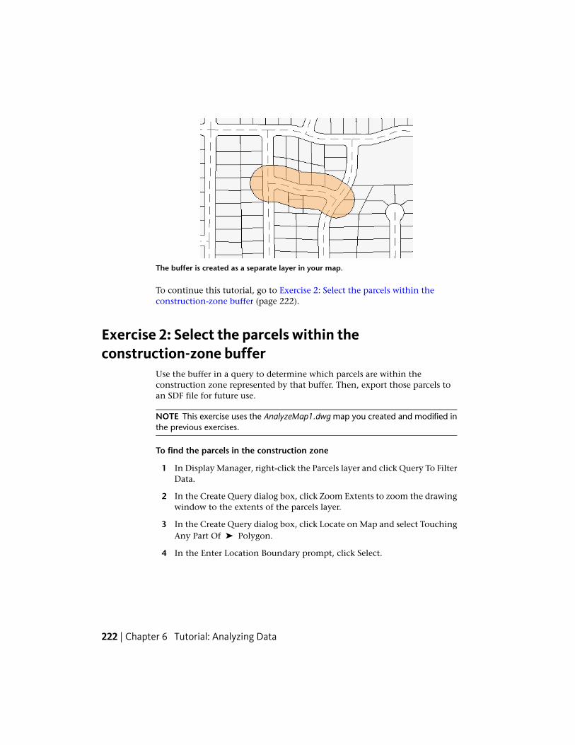
The buffer is created as a separate layer in your map.
To continue this tutorial, go to Exercise 2: Select the parcels within theconstruction-zone buffer (page 222).
Exercise 2: Select the parcels within theconstruction-zone buffer
Use the buffer in a query to determine which parcels are within theconstruction zone represented by that buffer. Then, export those parcels toan SDF file for future use.
NOTE This exercise uses the AnalyzeMap1.dwg map you created and modified inthe previous exercises.
To find the parcels in the construction zone
1 In Display Manager, right-click the Parcels layer and click Query To FilterData.
2 In the Create Query dialog box, click Zoom Extents to zoom the drawingwindow to the extents of the parcels layer.
3 In the Create Query dialog box, click Locate on Map and select TouchingAny Part Of ➤ Polygon.
4 In the Enter Location Boundary prompt, click Select.
222 | Chapter 6 Tutorial: Analyzing Data
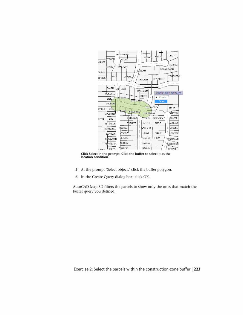
Click Select in the prompt. Click the buffer to select it as thelocation condition.
5 At the prompt "Select object," click the buffer polygon.
6 In the Create Query dialog box, click OK.
AutoCAD Map 3D filters the parcels to show only the ones that match thebuffer query you defined.
Exercise 2: Select the parcels within the construction-zone buffer | 223
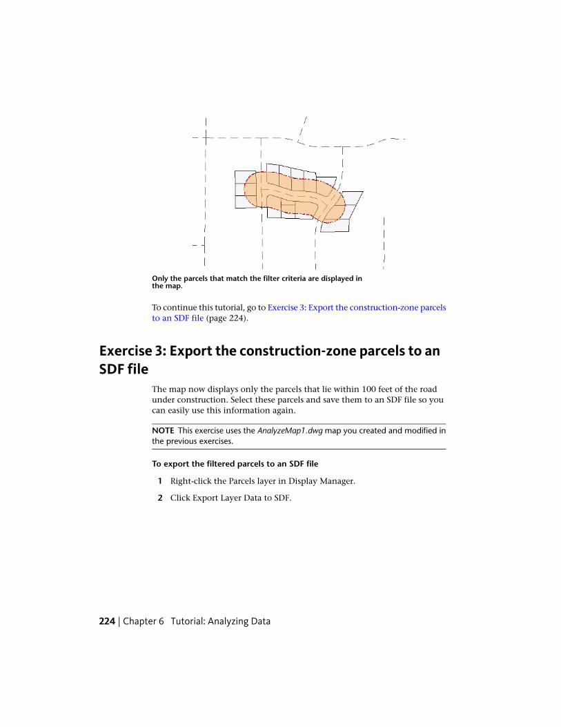
Only the parcels that match the filter criteria are displayed inthe map.
To continue this tutorial, go to Exercise 3: Export the construction-zone parcelsto an SDF file (page 224).
Exercise 3: Export the construction-zone parcels to anSDF file
The map now displays only the parcels that lie within 100 feet of the roadunder construction. Select these parcels and save them to an SDF file so youcan easily use this information again.
NOTE This exercise uses the AnalyzeMap1.dwg map you created and modified inthe previous exercises.
To export the filtered parcels to an SDF file
1 Right-click the Parcels layer in Display Manager.
2 Click Export Layer Data to SDF.
224 | Chapter 6 Tutorial: Analyzing Data
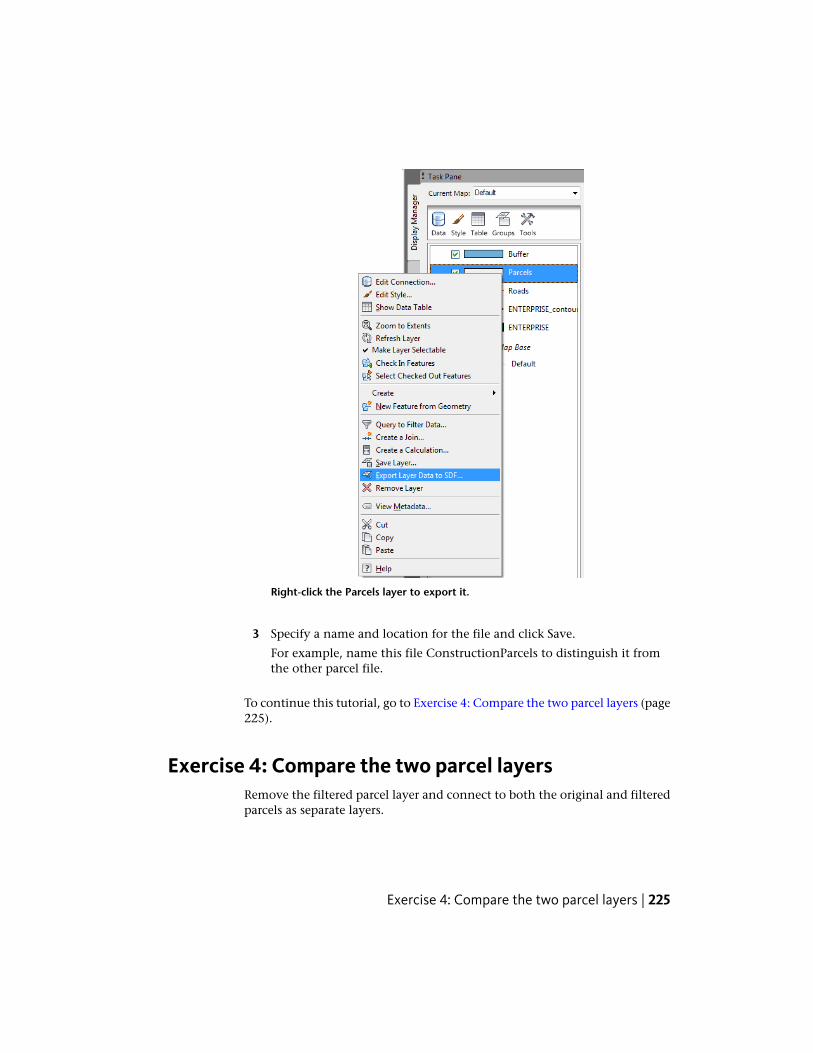
Right-click the Parcels layer to export it.
3 Specify a name and location for the file and click Save.
For example, name this file ConstructionParcels to distinguish it fromthe other parcel file.
To continue this tutorial, go to Exercise 4: Compare the two parcel layers (page225).
Exercise 4: Compare the two parcel layersRemove the filtered parcel layer and connect to both the original and filteredparcels as separate layers.
Exercise 4: Compare the two parcel layers | 225
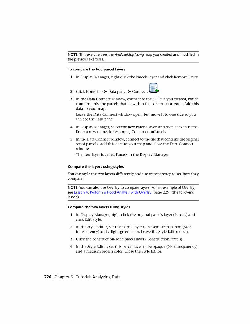
NOTE This exercise uses the AnalyzeMap1.dwg map you created and modified inthe previous exercises.
To compare the two parcel layers
1 In Display Manager, right-click the Parcels layer and click Remove Layer.
2 Click Home tab ➤ Data panel ➤ Connect.
3 In the Data Connect window, connect to the SDF file you created, whichcontains only the parcels that lie within the construction zone. Add thisdata to your map.
Leave the Data Connect window open, but move it to one side so youcan see the Task pane.
4 In Display Manager, select the new Parcels layer, and then click its name.Enter a new name, for example, ConstructionParcels.
5 In the Data Connect window, connect to the file that contains the originalset of parcels. Add this data to your map and close the Data Connectwindow.
The new layer is called Parcels in the Display Manager.
Compare the layers using styles
You can style the two layers differently and use transparency to see how theycompare.
NOTE You can also use Overlay to compare layers. For an example of Overlay,see Lesson 4: Perform a Flood Analysis with Overlay (page 229) (the followinglesson).
Compare the two layers using styles
1 In Display Manager, right-click the original parcels layer (Parcels) andclick Edit Style.
2 In the Style Editor, set this parcel layer to be semi-transparent (50%transparency) and a light green color. Leave the Style Editor open.
3 Click the construction-zone parcel layer (ConstructionParcels).
4 In the Style Editor, set this parcel layer to be opaque (0% transparency)and a medium brown color. Close the Style Editor.
226 | Chapter 6 Tutorial: Analyzing Data

5 In Display Manager, redisplay the surface raster image by selecting itsbox and the box for the contour layer.
6 In Display Manager, clear the check box for the buffer layer.
7 In Display Manager, click Groups and click Draw Order.
The name changes to Order and you can set the draw order of the layersin your map.
8 Make sure the draw order looks like the illustration:
Click Groups and click Draw Order to change thename of the button to Order. Use Order to changehow layers overlay each other.
Exercise 4: Compare the two parcel layers | 227

Where you are now
Your map now displays the raster image, overlaid with theroads, the original parcel layer, and the construction-zoneparcels.
To continue this tutorial, go to Exercise 5: Export the data to CSV for use ina report (page 228).
Exercise 5: Export the data to CSV for use in a reportDisplay the Data Table for the construction-zone parcels. Export the data toa comma-separated file. You can use the data in any way you like. For example,use it in a report, or to create a mailing list for the owners of theconstruction-zone parcels.
NOTE This exercise uses the AnalyzeMap1.dwg map you created and modified inthe previous exercises.
To export the construction-zone parcel data
1 In Display Manager, select the construction-zone parcel layer and clickTable.
2 In the Data Table, right-click the left-most column and click Select All.
3 Click Options (at the bottom of the table) and click Export.
228 | Chapter 6 Tutorial: Analyzing Data
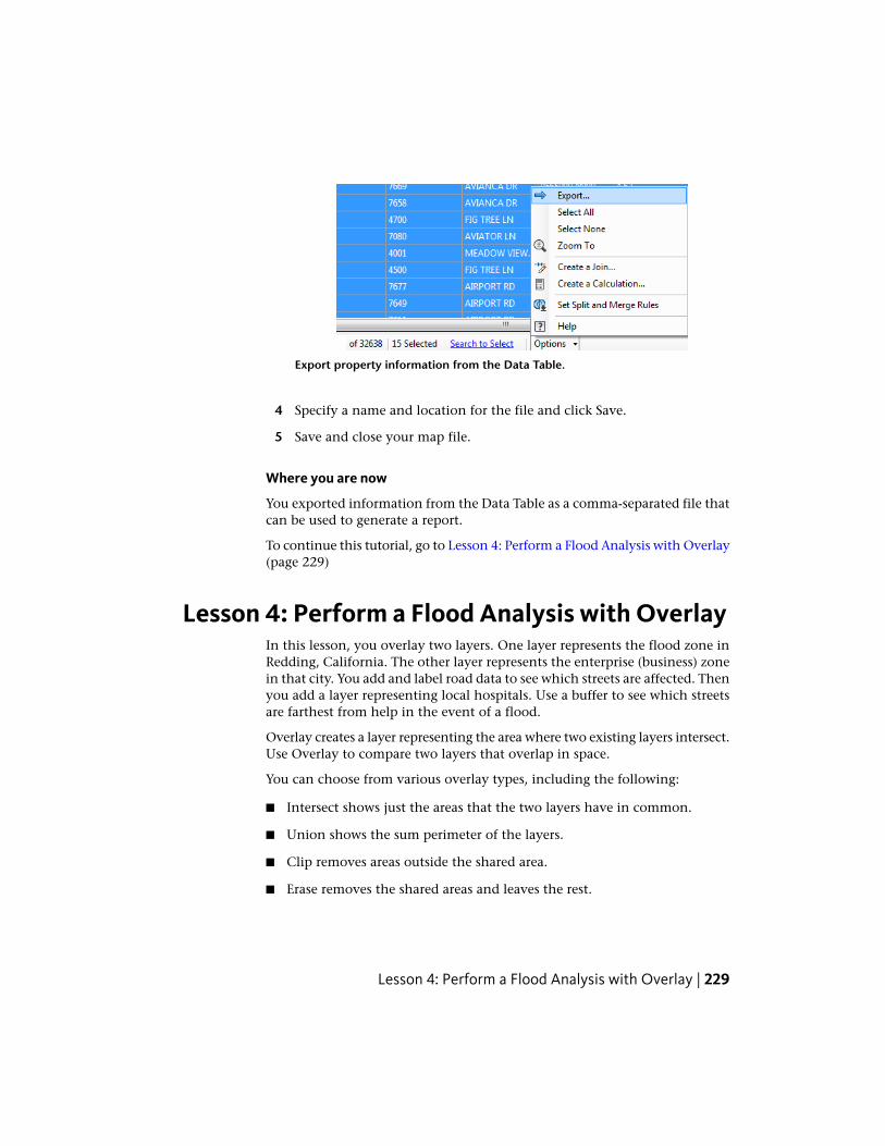
Export property information from the Data Table.
4 Specify a name and location for the file and click Save.
5 Save and close your map file.
Where you are now
You exported information from the Data Table as a comma-separated file thatcan be used to generate a report.
To continue this tutorial, go to Lesson 4: Perform a Flood Analysis with Overlay(page 229)
Lesson 4: Perform a Flood Analysis with OverlayIn this lesson, you overlay two layers. One layer represents the flood zone inRedding, California. The other layer represents the enterprise (business) zonein that city. You add and label road data to see which streets are affected. Thenyou add a layer representing local hospitals. Use a buffer to see which streetsare farthest from help in the event of a flood.
Overlay creates a layer representing the area where two existing layers intersect.Use Overlay to compare two layers that overlap in space.
You can choose from various overlay types, including the following:
■ Intersect shows just the areas that the two layers have in common.
■ Union shows the sum perimeter of the layers.
■ Clip removes areas outside the shared area.
■ Erase removes the shared areas and leaves the rest.
Lesson 4: Perform a Flood Analysis with Overlay | 229
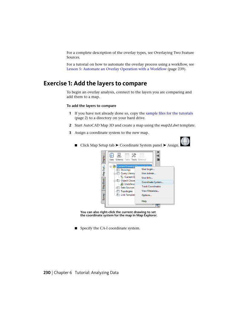
For a complete description of the overlay types, see Overlaying Two FeatureSources.
For a tutorial on how to automate the overlay process using a workflow, seeLesson 5: Automate an Overlay Operation with a Workflow (page 239).
Exercise 1: Add the layers to compareTo begin an overlay analysis, connect to the layers you are comparing andadd them to a map.
To add the layers to compare
1 If you have not already done so, copy the sample files for the tutorials(page 2) to a directory on your hard drive.
2 Start AutoCAD Map 3D and create a map using the map2d.dwt template.
3 Assign a coordinate system to the new map.
■ Click Map Setup tab ➤ Coordinate System panel ➤ Assign.
You can also right-click the current drawing to setthe coordinate system for the map in Map Explorer.
■ Specify the CA-I coordinate system.
230 | Chapter 6 Tutorial: Analyzing Data

4 Connect to the first data store.
■ Click Home tab ➤ Data panel ➤ Connect.
■ In the Data Connect window, under Data Connections By Provider,select Add SDF Connection.
■ Click next to the Source File field and navigate to the folder whereyou copied the sample files.
■ In the Open dialog box, select FLOODZONE.SDF and click Open.
■ In the Data Connect window, click Connect.
■ In the Data Connect window, click Add To Map.
5 Connect to the second data store.
■ With the Data Connect window still open, under Data ConnectionsBy Provider, select Add SDF Connection again.
■ Click next to the Source File field and navigate to the folder whereyou copied the sample files.
■ In the Open dialog box, select E_ZONE.SDF and click Open.
■ In the Data Connect window, click Connect.
■ In the Data Connect window, click Add To Map.
6 Click ➤ Save As. In your tutorials folder, name the fileAnalyzeMapOverlay.dwg and click OK.
To continue this tutorial, go to Exercise 2: Use an overlay to compare twolayers (page 231).
Exercise 2: Use an overlay to compare two layersCompare the two layers you added in the previous exercise. The overlay showsyou which parts of the enterprise zone lie within the flood zone.
NOTE This exercise uses the AnalyzeMapOverlay.dwg map you created in Exercise1: Add the layers to compare (page 230).
Exercise 2: Use an overlay to compare two layers | 231

To use an overlay to compare the two layers
1 Analyze tab ➤ Feature panel ➤ Feature Overlay
2 In the Sources and Overlay Type window of the Overlay Analysis dialogbox, do the following:
■ For Source, select E_zone (Polygons).
■ For Overlay, select floodzone (Polygons).
■ For Type, select Intersect.
■ Click Next.
3 In the Set Output And Settings window of the Overlay Analysis dialogbox, do the following:
■ Enter a location for the overlay layer SDF file.
■ Enter a name for the layer. This name appears in Display Manager.
■ For Sliver Tolerance, select Don’t Remove Slivers.Slivers are tiny polygons that can result from the overlay procedure.
■ Leave the remaining settings as they are and click Finish.
232 | Chapter 6 Tutorial: Analyzing Data
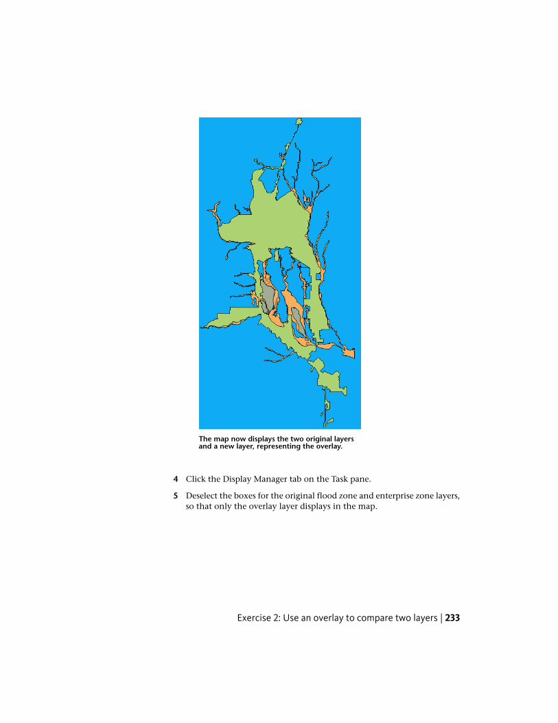
The map now displays the two original layersand a new layer, representing the overlay.
4 Click the Display Manager tab on the Task pane.
5 Deselect the boxes for the original flood zone and enterprise zone layers,so that only the overlay layer displays in the map.
Exercise 2: Use an overlay to compare two layers | 233

Hide all the layers except theoverlay.
6 Save the map.
To continue this tutorial, go to Exercise 3: Add and style a road layer (page234).
Exercise 3: Add and style a road layerYou can see the area of the enterprise zone that lies within the flood zone.However, it is hard to identify specific streets without a road map. In thislesson, you add a road layer and label it with street names. That way, you canidentify the streets in the flood zone more easily.
NOTE This exercise uses the AnalyzeMapOverlay.dwg map you created and modifiedin Exercise 2: Use an overlay to compare two layers (page 231).
To add roads to the map
1 Click Home tab ➤ Data panel ➤ Connect.
2 In the Data Connect window, under Data Connections By Provider, selectAdd SHP Connection.
234 | Chapter 6 Tutorial: Analyzing Data
3 Click next to the Source File Or Folder field and navigate to thefolder where you copied the sample files.
4 In the Open dialog box, select ROADS.SHP and click Open.
5 In the Data Connect window, click Connect.
6 In the Data Connect window, click Add To Map.
7 Close the Data Connect window.
To style the roads in the map
1 In Display Manager, select the Roads layer and click Style.
2 In the Style Editor, click the Style entry.
3 In the Style Line dialog box, change the road color to black and click OK.
4 In the Style Editor, click the Feature Label entry.
5 For Property To Display, select ST_NAME and click OK.
6 Close the Style Editor.
Exercise 3: Add and style a road layer | 235
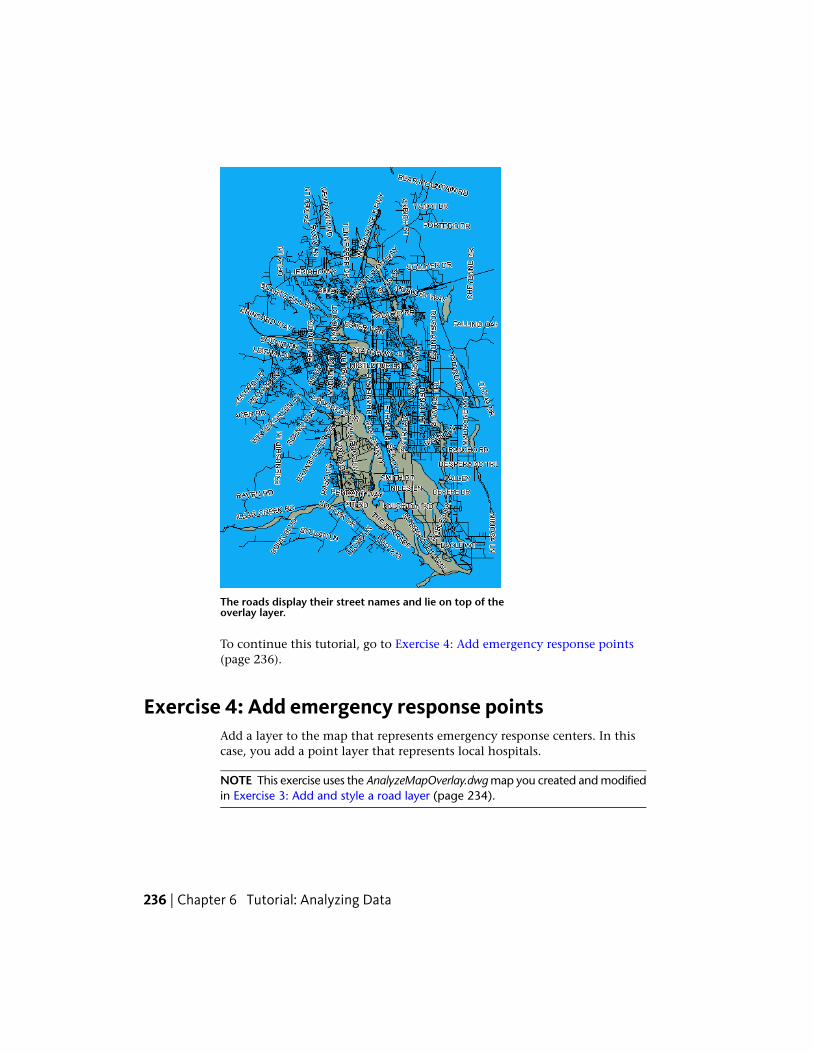
The roads display their street names and lie on top of theoverlay layer.
To continue this tutorial, go to Exercise 4: Add emergency response points(page 236).
Exercise 4: Add emergency response pointsAdd a layer to the map that represents emergency response centers. In thiscase, you add a point layer that represents local hospitals.
NOTE This exercise uses the AnalyzeMapOverlay.dwg map you created and modifiedin Exercise 3: Add and style a road layer (page 234).
236 | Chapter 6 Tutorial: Analyzing Data
To add the points representing emergency response centers
1 Click Home tab ➤ Data panel ➤ Connect
2 In the Data Connect window, under Data Connections By Provider, selectAdd SDF Connection.
3 Click next to the Source File field and navigate to the folder whereyou copied the sample files.
4 In the Open dialog box, select HOSPITAL.SDF and click Open.
5 In the Data Connect window, click Connect.
6 In the Data Connect window, click Add To Map.
To continue this tutorial, go to Exercise 5: Find streets that are far from ahospital (page 237).
Exercise 5: Find streets that are far from a hospitalUse a buffer to find areas of the enterprise zone that are within the flood zoneand are also more than 5 miles from a hospital. Use the hospital points as thebuffer origin and set the buffer distance to 5 miles.
NOTE This exercise uses the AnalyzeMapOverlay.dwg map you created and modifiedin Exercise 4: Add emergency response points (page 236).
To use a buffer to see which streets are far from a hospital
1 Click Analyze tab ➤ Feature panel ➤ Feature Buffer.
2 In the Create Buffer dialog box, click Select Features.
3 In your map, click each of the squares representing the two hospitals.Press Enter when both are selected.
You return to the Create Buffer dialog box, which now indicates that twofeatures are selected.
4 In the Create Buffer dialog box, set Distance to 5 and Units to Miles. ClickOK.
Exercise 5: Find streets that are far from a hospital | 237

Where you are now
The map now displays two large circles, each with a five-mile radius.The center of each circle is a hospital. Areas outside the circles are morethan 5 miles from either hospital. The street name labels help youdetermine which areas are most vulnerable when a flood occurs.
To continue this tutorial, go to Lesson 5: Automate an Overlay Operation witha Workflow (page 239).
238 | Chapter 6 Tutorial: Analyzing Data

Lesson 5: Automate an Overlay Operation with aWorkflow
In Lesson 4: Perform a Flood Analysis with Overlay (page 229), you comparedtwo SDF layers using an overlay. In this lesson, you automate that processwith a workflow.
Exercise 1: Edit a workflowA workflow automates a set of processes. You can specify the parameters forthe processes, or fill them in when you (or others) run the workflow.
In this lesson, you edit the predefined workflow that connects to two datastores and compares the resulting feature layers with an overlay. You willspecify the same data stores and overlay parameters that you used in Lesson4: Perform a Flood Analysis with Overlay (page 229).
To edit the workflow
1 In AutoCAD Map 3D, create a map.
■ Click ➤ New ➤ Drawing.
■ Select the map2d.dwt template and click Open.
2 Click Tools tab ➤ Workflow panel ➤ Edit.
3 In the Workflow Designer, expand the parallel activity at the top of theworkflow diagram.
Each entry within the parallel activity connects to one of the data storesyou need. Because the connections are parallel, AutoCAD Map 3Dperforms them both, even if the first one fails. If one of the connectionsfails, AutoCAD Map 3D tries it again until it times out.
Lesson 5: Automate an Overlay Operation with a Workflow | 239

Expand the parallel activity to see the activities inside it.
4 In the parallel activity, double-click the first Connect To An FDO DataStore activity.
5 Set the parameters for the first connection activity.
■ In the Connect To An FDO Data Store window, change the Providerto OSGeo.SDF.3.4.
■ Click next to File Name and navigate to the FLOODZONE.SDF file.
240 | Chapter 6 Tutorial: Analyzing Data
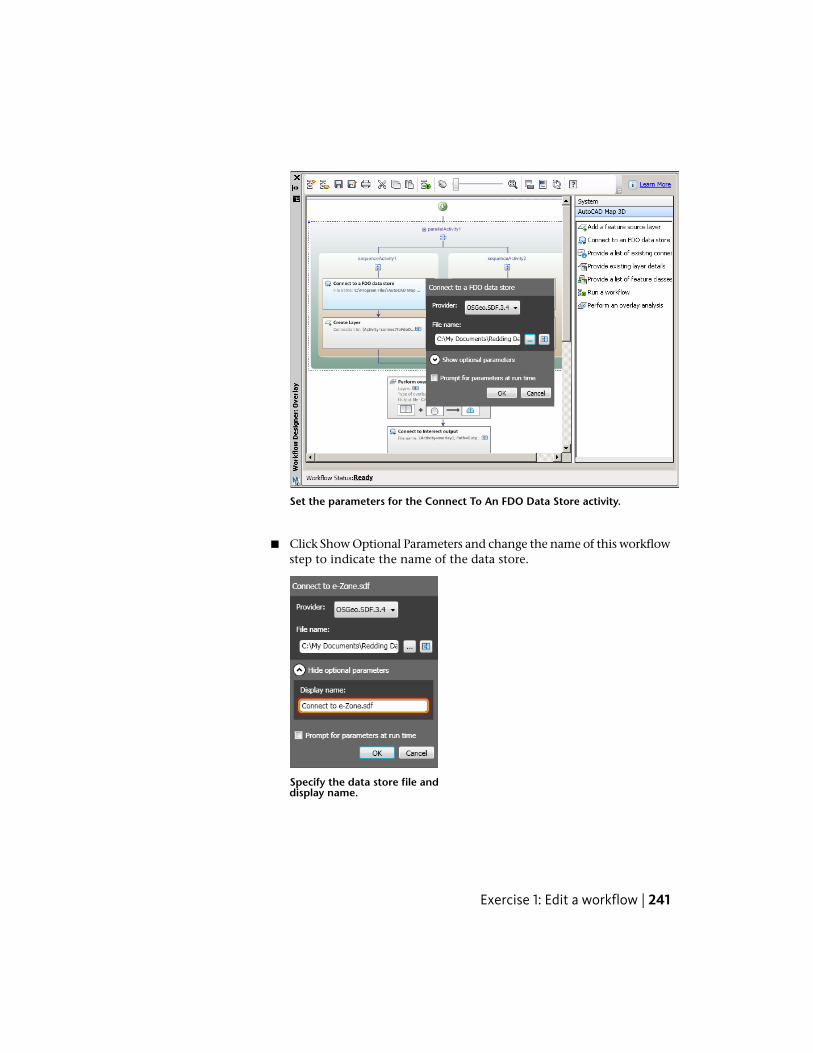
Set the parameters for the Connect To An FDO Data Store activity.
■ Click Show Optional Parameters and change the name of this workflowstep to indicate the name of the data store.
Specify the data store file anddisplay name.
Exercise 1: Edit a workflow | 241
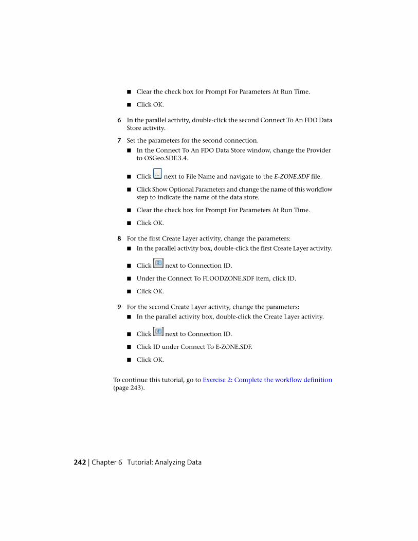
■ Clear the check box for Prompt For Parameters At Run Time.
■ Click OK.
6 In the parallel activity, double-click the second Connect To An FDO DataStore activity.
7 Set the parameters for the second connection.
■ In the Connect To An FDO Data Store window, change the Providerto OSGeo.SDF.3.4.
■ Click next to File Name and navigate to the E-ZONE.SDF file.
■ Click Show Optional Parameters and change the name of this workflowstep to indicate the name of the data store.
■ Clear the check box for Prompt For Parameters At Run Time.
■ Click OK.
8 For the first Create Layer activity, change the parameters:
■ In the parallel activity box, double-click the first Create Layer activity.
■ Click next to Connection ID.
■ Under the Connect To FLOODZONE.SDF item, click ID.
■ Click OK.
9 For the second Create Layer activity, change the parameters:
■ In the parallel activity box, double-click the Create Layer activity.
■ Click next to Connection ID.
■ Click ID under Connect To E-ZONE.SDF.
■ Click OK.
To continue this tutorial, go to Exercise 2: Complete the workflow definition(page 243).
242 | Chapter 6 Tutorial: Analyzing Data
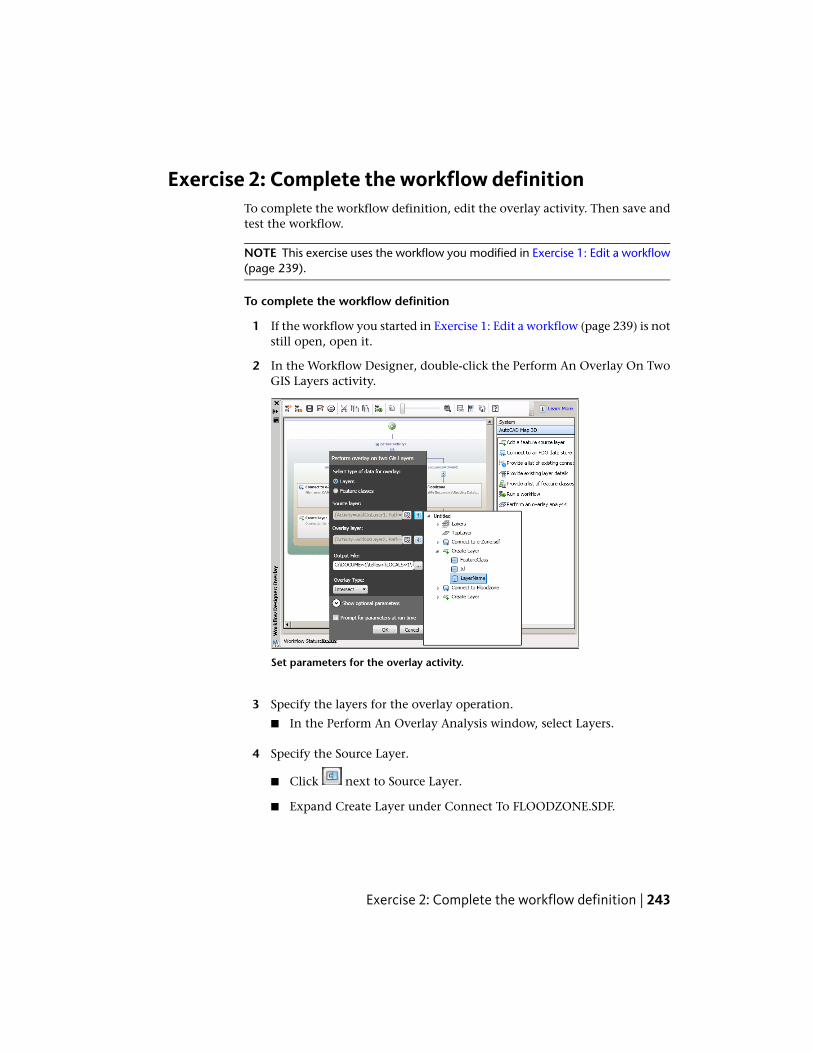
Exercise 2: Complete the workflow definitionTo complete the workflow definition, edit the overlay activity. Then save andtest the workflow.
NOTE This exercise uses the workflow you modified in Exercise 1: Edit a workflow(page 239).
To complete the workflow definition
1 If the workflow you started in Exercise 1: Edit a workflow (page 239) is notstill open, open it.
2 In the Workflow Designer, double-click the Perform An Overlay On TwoGIS Layers activity.
Set parameters for the overlay activity.
3 Specify the layers for the overlay operation.
■ In the Perform An Overlay Analysis window, select Layers.
4 Specify the Source Layer.
■ Click next to Source Layer.
■ Expand Create Layer under Connect To FLOODZONE.SDF.
Exercise 2: Complete the workflow definition | 243
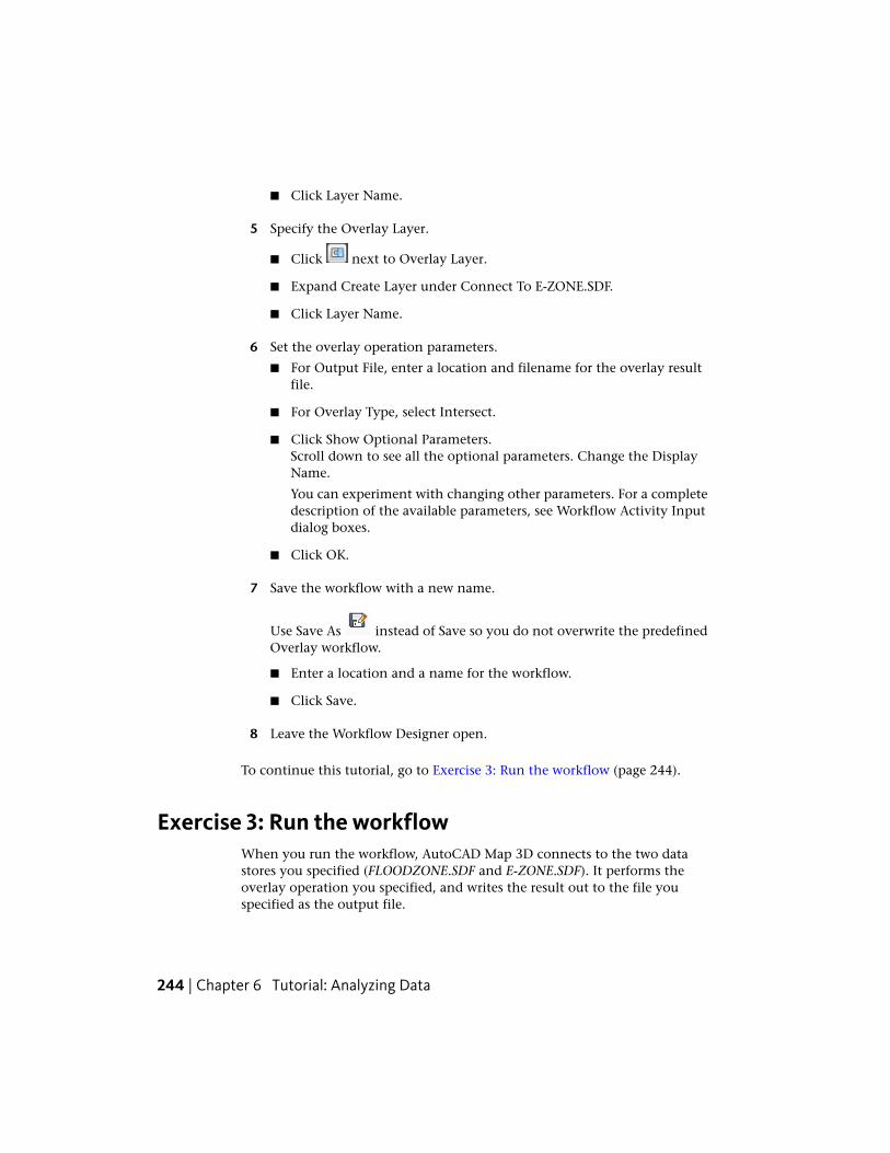
■ Click Layer Name.
5 Specify the Overlay Layer.
■ Click next to Overlay Layer.
■ Expand Create Layer under Connect To E-ZONE.SDF.
■ Click Layer Name.
6 Set the overlay operation parameters.
■ For Output File, enter a location and filename for the overlay resultfile.
■ For Overlay Type, select Intersect.
■ Click Show Optional Parameters.Scroll down to see all the optional parameters. Change the DisplayName.
You can experiment with changing other parameters. For a completedescription of the available parameters, see Workflow Activity Inputdialog boxes.
■ Click OK.
7 Save the workflow with a new name.
Use Save As instead of Save so you do not overwrite the predefinedOverlay workflow.
■ Enter a location and a name for the workflow.
■ Click Save.
8 Leave the Workflow Designer open.
To continue this tutorial, go to Exercise 3: Run the workflow (page 244).
Exercise 3: Run the workflowWhen you run the workflow, AutoCAD Map 3D connects to the two datastores you specified (FLOODZONE.SDF and E-ZONE.SDF). It performs theoverlay operation you specified, and writes the result out to the file youspecified as the output file.
244 | Chapter 6 Tutorial: Analyzing Data

AutoCAD Map 3D creates the specified layers in your map. If you open theData Connect window, you can see that the connections have been made.
NOTE This exercise uses the workflow you modified in Exercise 2: Complete theworkflow definition (page 243).
To run the workflow
1 If the Workflow Designer is not still open from Exercise 2: Complete theworkflow definition (page 243), open it.
■ In the list on the Tools tab, Workflow panel, select the workflow youcreated.
■ Click Edit.
2 In the Workflow Designer, click .
Green check marks appear in the upper-right corners of each workflowstep.
3 Close the Workflow Designer by clicking the x in its title bar.
The source and overlay layers are added to the map, as well as the resultof the overlay. The Intersect layer represents the area of the enterprisezone that lies within the flood zone.
4 Turn off all layers except Intersect to see the intersection of the two areas.
To turn off a layer, clear its check box in Display Manager.
Exercise 3: Run the workflow | 245

Where you are now
The workflow you created has performed an overlay operation. The erased dataand intersecting data that result from the overlay are each stored as new datastores and added to your map.
246 | Chapter 6 Tutorial: Analyzing Data
Tutorial: Managing DataFrom Different Sources
About the Managing Data TutorialAn AutoCAD Map 3D map can contain many types of information, includingDWG objects you query in from drawing files and features from multiplegeospatial data sources:
■ Oracle, SQL Server, MySQL, and ArcSDE database stores
■ SDF and SHP files
■ ODBC databases
Once you add data to your map, you can convert it from one data format toanother. For example, you can do the following:
■ Make DWG data available in a geospatial format for other organizations.
■ Move data for your organization into a geospatial environment.
■ Bring geospatial data into a drawing file.
■ Use options that are available only for drawing data or only for geospatialdata, and then return the data to its native format.For example, you can import geospatial data to convert it to DWG formatand then use drawing cleanup commands (which are not available forgeospatial data). You can convert DWG data to geospatial format and usethe split/merge commands to assign attribute data to the split or mergedfeatures. These commands are not available for drawing objects.
7
247

■ Save a map in DWG format so AutoCAD users (without access to AutoCADMap 3D) can edit map data.
Select the appropriate method to move data into or out of a map:
Update OptionsMethod
If you change the objects, you can updatethe original drawing or not.
Attach a drawing to your map and thenquery in the objects to use.
You can maintain a live connection to thedata, or work offline and update your datastore when you finish.
Connect to geospatial (FDO) data.
When you use this option, you do not af-fect the original data store. Changes in thatdata store do not change your map.
Import data into your map, automaticallyconverting it to DWG format. Importinginserts a "snapshot" of the data. You canimport from various geospatial sources.
The original data is unchanged.Export drawing objects to various formats.No geospatial features are exported, butyou can save all the features and objectsin your map to AutoCAD DWG format andthen export it.
The original geospatial data source is un-changed.
Use Bulk Copy to convert geospatial datato another geospatial format.
The original DWG data is unchanged.Export your map or individual drawinglayers to the Autodesk SDF format, or toSHP, ArcSDE, or Oracle. Then use BulkCopy to move it to other formats.
Converting Drawing Layers to Feature Classes
In an AutoCAD drawing, you can use layers to organize information. Forexample, an AutoCAD drawing can contain separate layers for roads, parcels,and so on. Geospatial data stores use schemas for this purpose. In a schema,each feature class can serve the same purpose as a drawing layer.
SDF is a proprietary Autodesk format. It supports a schema that can includemultiple feature classes within a single file, the same way that a single drawingcan include multiple drawing layers. In this tutorial, you create an SDF filewith a schema whose feature classes reflect the layer structure of a drawing
248 | Chapter 7 Tutorial: Managing Data From Different Sources

file. Each layer in the drawing file becomes a feature class in the SDF file. whenyou export it.
Use the Export dialog box to map each layer to a target feature class. You canalso convert object data to geospatial attribute data. Once you set up themapping, you can save your settings as a profile, allowing you to use thesettings over and over again.
Using the Resulting SDF File
Once the data is stored in the SDF file, you can connect to that SDF data store.Add the SDF features to a map as Display Manager layers.
One advantage of geospatial data stores is the ease with which you can controlattribute data (called “properties” for feature classes). In this tutorial, you adda constrained (page 309) property to a feature class in the SDF schema.
A constrained property can have only one of a set of predefined values, oronly values within a particular range. For example, you can define a Zoningproperty whose values can be only Residential, Commercial, or Public.
Moving SDF Data to a Different Geospatial Format
Once data is in a geospatial format, you can use Bulk Copy to move it to adifferent geospatial format. For example, you can copy SDF data to a set ofSHP files.
Converting the Data to DWG Format
If needed, you can reimport your changes in DWG format. If you create atemplate file specifying the original layers for the data, you can place eachfeature class into its appropriate drawing layer. The data then uses the stylinginformation for the drawing layer, rather than the styling you applied to theDisplay Manager layer.
About the Managing Data Tutorial | 249
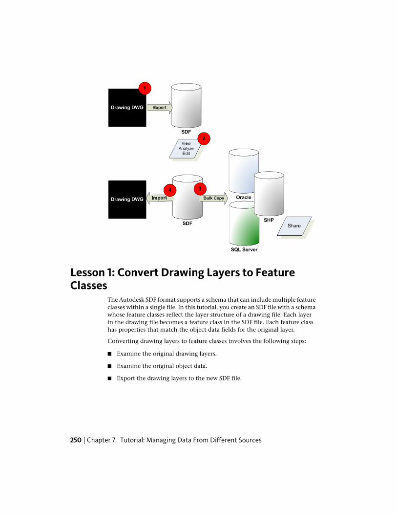
Lesson 1: Convert Drawing Layers to FeatureClasses
The Autodesk SDF format supports a schema that can include multiple featureclasses within a single file. In this tutorial, you create an SDF file with a schemawhose feature classes reflect the layer structure of a drawing file. Each layerin the drawing file becomes a feature class in the SDF file. Each feature classhas properties that match the object data fields for the original layer.
Converting drawing layers to feature classes involves the following steps:
■ Examine the original drawing layers.
■ Examine the original object data.
■ Export the drawing layers to the new SDF file.
250 | Chapter 7 Tutorial: Managing Data From Different Sources
Exercise 1: Examine the original drawing layersYou create an SDF file with a schema whose feature classes reflect the layerstructure of a drawing file. Examine the original drawing layers, so you cancheck the resulting SDF file to see if it is structured correctly.
To examine the drawing layers
1 If you have not already done so, copy the sample files for the tutorialsto a directory on your hard drive. See Lesson 1: Get Ready to Use theTutorials (page 1).
2 Start AutoCAD Map 3D.
3 Click ➤ Open ➤ Drawing. Open the sample map calledDWGMap.dwg.
Exercise 1: Examine the original drawing layers | 251
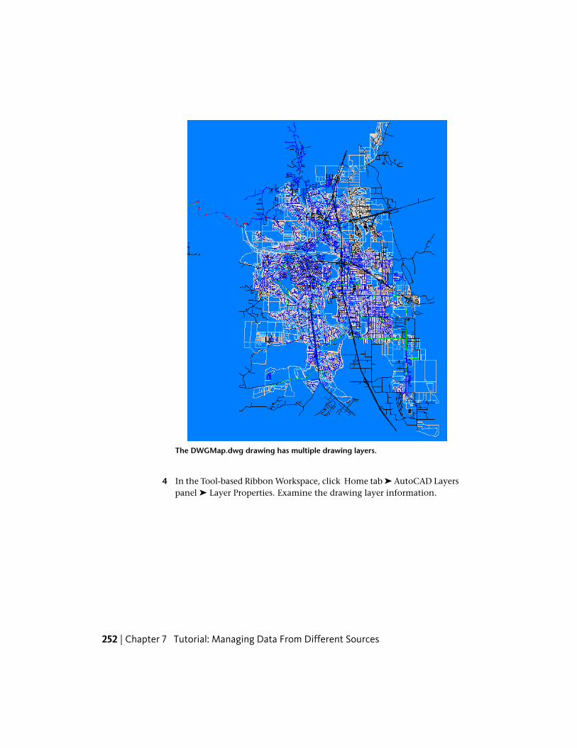
The DWGMap.dwg drawing has multiple drawing layers.
4 In the Tool-based Ribbon Workspace, click Home tab ➤ AutoCAD Layerspanel ➤ Layer Properties. Examine the drawing layer information.
252 | Chapter 7 Tutorial: Managing Data From Different Sources

The layers in the drawing are listed, along with their properties.
To continue this tutorial, go to Exercise 2: Examine the object data (page 253)
Exercise 2: Examine the object dataThe drawing layers in your DWG file become the feature classes in the newschema. The object data properties in the drawing determine the propertiesfor each feature class. Use the Properties palette to see the object data.
NOTE This exercise uses the DWGMap.dwg map file you opened in Exercise 1:Examine the original drawing layers (page 251).
To view the object data fields
1 In the map, zoom in close enough to see individual objects.
Use the zoom commands on the View tab.
2 Select one of the pink polylines in the map.
The Quick Properties panel displays a short list of properties.
3 Close Quick Properties, right-click the polygon, and click Properties.
4 Notice that the color for these polylines is ByLayer. Check the lower areaof the Design tab of the Properties palette to see the object data.
The pink polylines represent parcels and have object data related toaddress, area, value, and so on.
Exercise 2: Examine the object data | 253
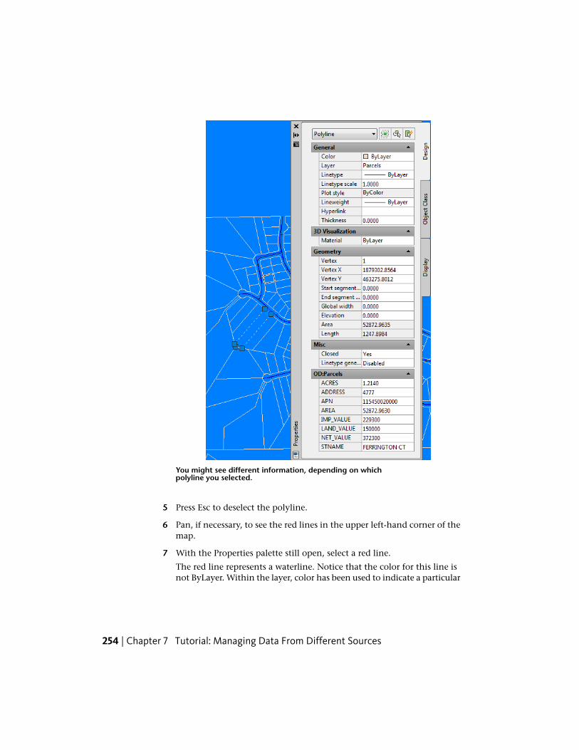
You might see different information, depending on whichpolyline you selected.
5 Press Esc to deselect the polyline.
6 Pan, if necessary, to see the red lines in the upper left-hand corner of themap.
7 With the Properties palette still open, select a red line.
The red line represents a waterline. Notice that the color for this line isnot ByLayer. Within the layer, color has been used to indicate a particular
254 | Chapter 7 Tutorial: Managing Data From Different Sources

type of waterline. In this case it indicates size. Red waterlines have adiameter from 26 through 48 inches.
8 Deselect the red line and pan to the lower right side of the drawing.
9 Select a green line.
The green line is also a waterline, but it is a different size. Green waterlinesare from 13 through 24 inches in diameter. Blue waterlines are from 1through 12 inches in diameter.
10 Press Esc to ensure that no objects are selected.
The Properties palette displays “No selection” in the top field when youdeselect all objects.
11 Close the Properties palette.
To continue this tutorial, go to Exercise 3: Export the drawing layers to SDF -Select the layers (page 255)
Exercise 3: Export the drawing layers to SDF - Select thelayers
In this exercise, you export the drawing layers from the original DWG file toa new SDF file. The original drawing layers become geospatial features withproperties that reflect the object data and AutoCAD properties.
Use the Export dialog box to map each layer to a target feature class andconvert object data and properties to geospatial attribute data. Once you setup the mapping, you can save your settings as a profile, allowing you to usethe settings over and over again.
You cannot maintain styling information when you export drawing objectsto SDF, but you can include object attributes. When you export the Waterlinelayer, you map the Color attribute to a SIZE property.
The Export dialog box has three tabs. The following exercises describe thesteps to take on each tab.
NOTE This exercise uses the DWGMap.dwg map file you opened and modified inExercise 1: Examine the original drawing layers (page 251).
Exercise 3: Export the drawing layers to SDF - Select the layers | 255

To select the layers to export to SDF
1 Click Output tab ➤ Map Data Transfer panel ➤ As SDF.
2 In the Save dialog box, specify a location and a name for the new SDFfile and click OK.
Make a note of the file name and location, so you can connect to thisfile later.
3 In the Export dialog box, on the Selection tab, click Select All.
4 Leave the Export dialog box open for the next exercise.
To continue this tutorial, go to Exercise 4: Export the drawing layers to SDF -Map object data to feature class properties (page 256).
Exercise 4: Export the drawing layers to SDF - Map objectdata to feature class properties
Use the Feature Class tab to map the properties for each layer to its resultingfeature class in the SDF file. You can specify some attributes as sharedproperties: all resulting feature classes have these properties. For example,Lineweight and Linestyle would apply to every feature class. You can specifyother attributes as specific to a particular feature class. For example, Addresswould apply to Parcels only.
NOTE This exercise uses the DWGMap.dwg map file you opened and modified inExercise 1: Examine the original drawing layers (page 251).
To specify the properties for the SDF feature classes
1 In the Export dialog box, on the Feature Class tab, click Create MultipleClasses Based On A Drawing Object. For Drawing Object To Use, selectLayer.
256 | Chapter 7 Tutorial: Managing Data From Different Sources

The table in the dialog box updates to show the layer names andfeature class names to use.
2 Deselect layer 0.
3 Click Select Attributes.
Attributes you specify here are assigned to every feature class in the SDFfile. So select only attributes that are appropriate for all of them. Forexample, you can select general properties, which include things likeLineweight, but not object data properties, which are specific to eachfeature class.
4 In the Select Attributes dialog box, expand the Object Properties itemand the AcDbEntity and General items.
5 Select the boxes for Lineweight and Linetype and click OK.
Exercise 4: Export the drawing layers to SDF - Map object data to feature class properties | 257
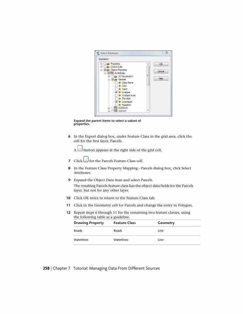
Expand the parent items to select a subset ofproperties.
6 In the Export dialog box, under Feature Class in the grid area, click thecell for the first layer, Parcels.
A button appears at the right side of the grid cell.
7 Click for the Parcels Feature Class cell.
8 In the Feature Class Property Mapping - Parcels dialog box, click SelectAttributes.
9 Expand the Object Data item and select Parcels.
The resulting Parcels feature class has the object data fields for the Parcelslayer, but not for any other layer.
10 Click OK twice to return to the Feature Class tab.
11 Click in the Geometry cell for Parcels and change the entry to Polygon.
12 Repeat steps 6 through 11 for the remaining two feature classes, usingthe following table as a guideline.
GeometryFeature ClassDrawing Property
LineRoadsRoads
LineWaterlinesWaterlines
258 | Chapter 7 Tutorial: Managing Data From Different Sources

13 Leave the Export dialog box open for the next exercise.
To continue this tutorial, go to Exercise 5: Export the drawing layers to SDF -Map drawing properties to feature class properties (page 259).
Exercise 5: Export the drawing layers to SDF - Mapdrawing properties to feature class properties
The Feature Class tab lets you map AutoCAD drawing properties to propertiesin the SDF feature classes as well. If you have used color, lineweight, or linetype to represent object characteristics within a layer, you can map theseproperties to the characteristics they represent. In this drawing, you map colorto a waterline size. You can map each waterline color to a separate featureproperty.
NOTE This exercise uses the DWGMap.dwg map file you opened and modified inExercise 1: Examine the original drawing layers (page 251).
To map drawing properties to feature class properties
1 On the Feature Class tab of the Export dialog box, click in the FeatureClass cell for Waterlines.
2 Click the button that appears in the cell.
3 In the Feature Class Property Mapping - Waterlines dialog box, click SelectAttributes.
4 Expand the Properties item at the top of the list.
5 Select COLOR and click OK.
6 In the Feature Class Property Mapping - Waterlines dialog box, in theFeature Class Properties cell for COLOR, enter Size.
In the exported SDF file, waterline objects with a COLOR property havea Size property instead.
7 Click the .COLOR cell to see the button.
8 Click the .COLOR button.
9 In the New Property Data Type dialog box, change the Data Type to Stringand click OK.
Exercise 5: Export the drawing layers to SDF - Map drawing properties to feature class properties | 259
The new Size property has a value that consists of a text string.
10 In the Property Value Mapping dialog box, select the box for each color(on the left side of the dialog box).
Specify what each color means. The text string you type is the value foreach waterline’s Size property. Red lines become Large waterlines in theSDF file.
11 Classify the waterline sizes as Small, Medium, and Large. Use this tableas a guideline:
SizeColor
LargeRed
MediumGreen
SmallBlue
260 | Chapter 7 Tutorial: Managing Data From Different Sources

Map the .COLOR property values to the feature class properties.
12 Click OK twice to return to the Export dialog box.
13 Leave the Export dialog box open for the next exercise.
Exercise 5: Export the drawing layers to SDF - Map drawing properties to feature class properties | 261

To continue this tutorial, go to Exercise 6: Export the drawing layers to SDF -Set export options (page 262).
Exercise 6: Export the drawing layers to SDF - Set exportoptions
As the final step in the export operation, set the export options. Save yoursettings as a profile so you can quickly execute this export operation againlater.
NOTE This exercise uses the DWGMap.dwg map file you opened and modified inExercise 1: Examine the original drawing layers (page 251).
To specify options for the export operation
1 In the Export dialog box, on the Options tab, select Treat Closed PolylinesAs Polygons.
Checking this option insures that polygon objects drawn as closedpolylines are still be treated as polygons in the exported file.
2 Under Saved Profiles, click Save.
3 Specify a location and name for these export settings and click Save.
4 In the Export dialog box, click OK to export the data.
The Export Progress dialog box displays the status of the export operation.
5 Close the map file.
Where you are now
You exported DWG layers to Autodesk SDF format, creating feature classesthat reflect the layers and object data in your original drawing file.
To continue this tutorial, go to Lesson 2: Use the Resulting SDF Files (page262).
Lesson 2: Use the Resulting SDF FilesConnect to the SDF file you created and edit the objects in the map asgeospatial features.
262 | Chapter 7 Tutorial: Managing Data From Different Sources

Geospatial features have options in AutoCAD Map 3D that drawing objectsdo not have. For example, you can add properties to the feature classes in yourSDF file. In this lesson, you add a constrained (page 309) property. Constrainedproperties can have only the values you specify: values within a particularrange or within a list you specify.
NOTE If you import the SDF file instead of connecting to it, the data comes backin as drawing objects instead of geospatial data. Connecting to the data leaves itin its current format.
This lesson involves the following steps:
■ Create a map.
■ Connect to the new SDF data.
■ Add a property.
Exercise 1: Create a mapCreate a map file.
To create a map file
1 Create a map using the map2d.dwt template.
2 Assign a coordinate system to the new map.
■ Switch the Task pane to Map Explorer.
■ Right-click the Current Drawing entry and click Coordinate System.
■ Specify the CA-I coordinate system.
Exercise 1: Create a map | 263

Set the coordinate system for a new map from MapExplorer.
3 Save your file.
To continue this tutorial, go to Exercise 2: Connect to the new SDF data (page264).
Exercise 2: Connect to the new SDF dataConnect to the SDF file you created.
NOTE This exercise uses the map you created in the previous exercise, and theSDF file you saved in Lesson 1: Convert Drawing Layers to Feature Classes (page250).
To connect to the new SDF file
1 In Display Manager, click Data ➤ Connect To Data.
264 | Chapter 7 Tutorial: Managing Data From Different Sources
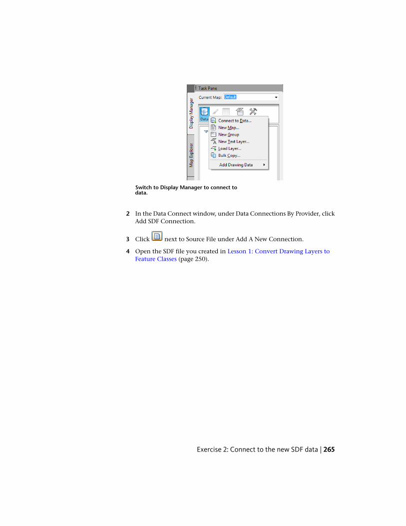
Switch to Display Manager to connect todata.
2 In the Data Connect window, under Data Connections By Provider, clickAdd SDF Connection.
3 Click next to Source File under Add A New Connection.
4 Open the SDF file you created in Lesson 1: Convert Drawing Layers toFeature Classes (page 250).
Exercise 2: Connect to the new SDF data | 265
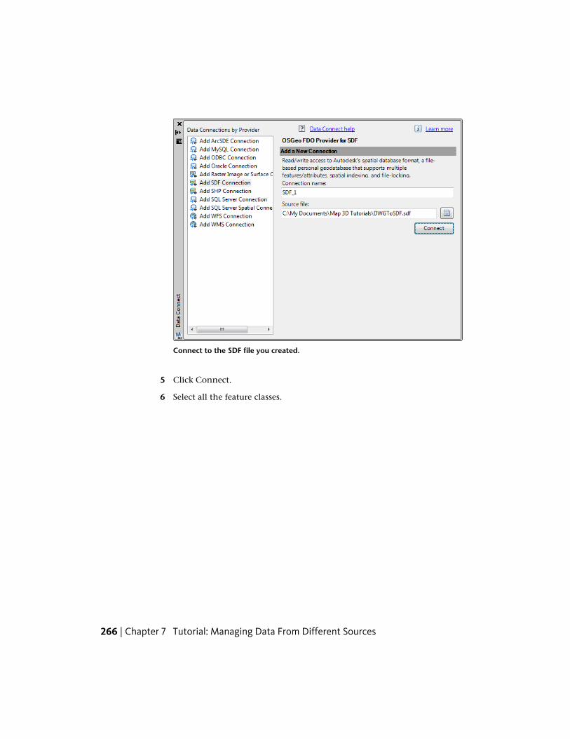
Connect to the SDF file you created.
5 Click Connect.
6 Select all the feature classes.
266 | Chapter 7 Tutorial: Managing Data From Different Sources

Each layer from your original map is listed as a separatefeature class.
7 Click Add To Map.
8 Close the Data Connect window.
To continue this tutorial, go to Exercise 3: Edit the schema (page 267).
Exercise 3: Edit the schemaIn this lesson, you examine the feature classes you created. You view theattribute data in the Data Table. Then, you add a feature class property usingthe Schema Editor.
NOTE This exercise uses the map you modified in Exercise 2: Connect to the newSDF data (page 264).
Exercise 3: Edit the schema | 267

To examine the attribute data
1 In the Task pane, switch to the Display Manager tab, select the Waterlineslayer and click Table.
NOTE In this example, the Data Table was undocked by dragging it awayfrom the edge of the window.
The general properties and the object data specific to Waterlines appear in the DataTable.
2 In the Data Table, examine the properties for the Waterlines layer.
The .COLOR properties have been translated to a new Size property.
3 Close the Data Table.
To continue this tutorial, go to Exercise 4: Add a property (page 268).
Exercise 4: Add a propertyA set of feature classes and their properties is called a schema. The schemacan have properties that are constrained (page 309). The constraints determinewhich objects you can add to a particular feature class. For example, to beadded to the Roads feature class, an object must be a line. Properties are like
268 | Chapter 7 Tutorial: Managing Data From Different Sources

attributes—they are characteristics of all objects in the feature class. Forexample, a Roads feature class property can specify the number of lanes it has,or its speed limit. The values vary, but all Roads features have a speed limitand a certain number of lanes.
You cannot change the schemas for all data source types, but you can edit theschemas for SDF files. In this lesson, you edit an SDF schema to add a propertyto the Roads feature class. The new property is constrained, so only certainvalues are valid for it.
NOTE This exercise uses the map you modified in Exercise 2: Connect to the newSDF data (page 264).
Properties that are constrained to ranges of values
You can specify that only values within a particular range are valid. You caninclude or exclude each extreme of the range: the lowest possible value andthe highest. For example, you can make a range 1 - 100 inclusive. You canspecify a range of any value higher than 1 and lower than 100, but not 1 or100. You can specify any combination.
To add a property to the Roads feature class that is constrained by range
1 Switch the Task pane to Map Explorer.
2 Select the SDF data source at the top of the pane.
3 Click Schema ➤ Edit Schema.
Edit the SDF schema.
Exercise 4: Add a property | 269
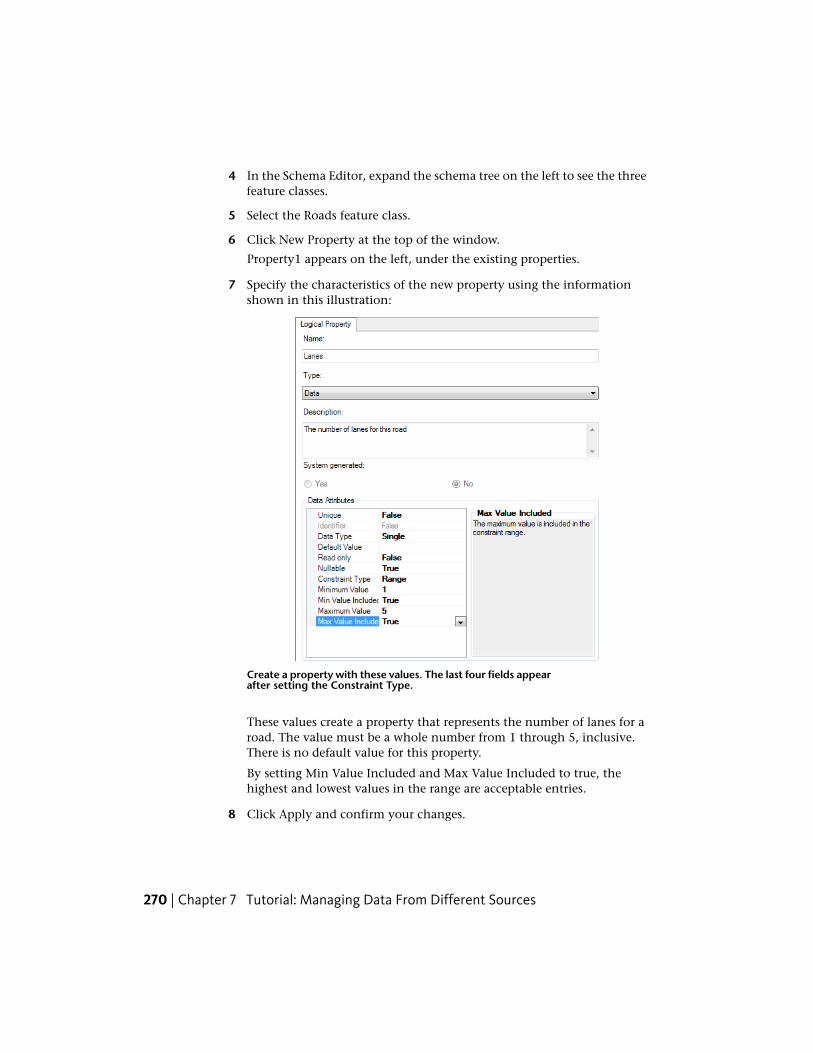
4 In the Schema Editor, expand the schema tree on the left to see the threefeature classes.
5 Select the Roads feature class.
6 Click New Property at the top of the window.
Property1 appears on the left, under the existing properties.
7 Specify the characteristics of the new property using the informationshown in this illustration:
Create a property with these values. The last four fields appearafter setting the Constraint Type.
These values create a property that represents the number of lanes for aroad. The value must be a whole number from 1 through 5, inclusive.There is no default value for this property.
By setting Min Value Included and Max Value Included to true, thehighest and lowest values in the range are acceptable entries.
8 Click Apply and confirm your changes.
270 | Chapter 7 Tutorial: Managing Data From Different Sources

The "Property1" entry on the left is updated to show the new name.
9 Click OK and confirm your changes to close the Schema Editor.
To continue this tutorial, go to Exercise 5: Populate the new property withvalues (page 271).
Exercise 5: Populate the new property with valuesAfter you add a property to a feature class, you enter the values for thatproperty for each feature in the feature class.
NOTE This exercise uses the map you modified in Exercise 2: Connect to the newSDF data (page 264).
To populate the new properties with data
1 Expand the SDF entry in Map Explorer until you see its three featureclasses. Select Roads and click Table.
2 In the Data Table, scroll all the way to the right to see the new property.
3 Enter the number of lanes for a few roads.
If you enter a value that is outside the allowable range and click outside the field, awarning is displayed.
Exercise 5: Populate the new property with values | 271
4 Close the Data Table.
Where you are now
You connected to the SDF file you created earlier and added a new propertyto its schema. You entered values for the new property in the Data Table.
To continue this tutorial, go to Lesson 3: Move SDF Data to a DifferentGeospatial Format (page 272).
Lesson 3: Move SDF Data to a Different GeospatialFormat
Use Bulk Copy to move the Roads data in your map from the SDF format itcurrently uses to ESRI SHP format.
While SDF files can contain multiple feature classes, each SHP file can containonly a single feature class. The Bulk Copy operation creates a set of new SHPfiles in a folder that you create.
NOTE You can use Bulk Copy to move data between geospatial formats, but youcannot use it to move data to or from DWG format.
NOTE This exercise uses the map you created with the map2d.dwt template andmodified in Lesson 2: Use the Resulting SDF Files (page 262).
Exercise 1: Connect to a new SHP file folderCreate a new, empty folder to contain the SHP files. To convert and copy datato the SHP format, you must be connected to this folder. You use Data Connectto establish connections to data stores, even when you do not add anythingto the map from the data store.
NOTE This exercise uses the map you created with the map2d.dwt template andmodified in Lesson 2: Use the Resulting SDF Files (page 262).
To create and connect to the folder
1 Use Windows Explorer to navigate to the location where you copied yoursample tutorial files.
2 Create a folder for the SHP files.
272 | Chapter 7 Tutorial: Managing Data From Different Sources

3 In AutoCAD Map 3D, switch the Task pane to Display Manager.
4 Click Data ➤ Connect To Data.
5 On the left side of the Data Connect dialog box, click Add SHPConnection.
6 On the right side of the Data Connect dialog box, click the folder icon(not the file icon). Select the folder you created and click OK.
Click the folder icon next to Source File Or Folder.
Click Connect and close the Data Connect window without addinganything to your map.
To continue this tutorial, go to Exercise 2: Use Bulk Copy to move an SDFlayer to SHP format (page 273).
Exercise 2: Use Bulk Copy to move an SDF layer to SHPformat
Copy the Roads layer from SDF format to SHP format using the Bulk Copyfeature.
NOTE This exercise uses the map you created with the map2d.dwt template andmodified in Exercise 1: Connect to a new SHP file folder (page 272).
Exercise 2: Use Bulk Copy to move an SDF layer to SHP format | 273

To copy the Roads layer to SHP format
1 In the Task pane, switch to Map Explorer. Select the SDF_1 schema.
2 Click Tools ➤ Bulk Copy.
Use Bulk Copy to convert data fromone geospatial format to another.
3 On the left side of the Bulk Copy dialog box, for Source, select the SDF_1connection.
4 In the list that displays on the left side of the window, select the box forSchema1.
5 On the right side of the Bulk Copy window, for Target, select the SHP_1connection.
6 Under Ignore The Following Errors During The Copy Process, select allthe items.
7 Click Copy Now.
NOTE If you see messages indicating that some property names are too long,shorten them and click Copy Now again.
274 | Chapter 7 Tutorial: Managing Data From Different Sources
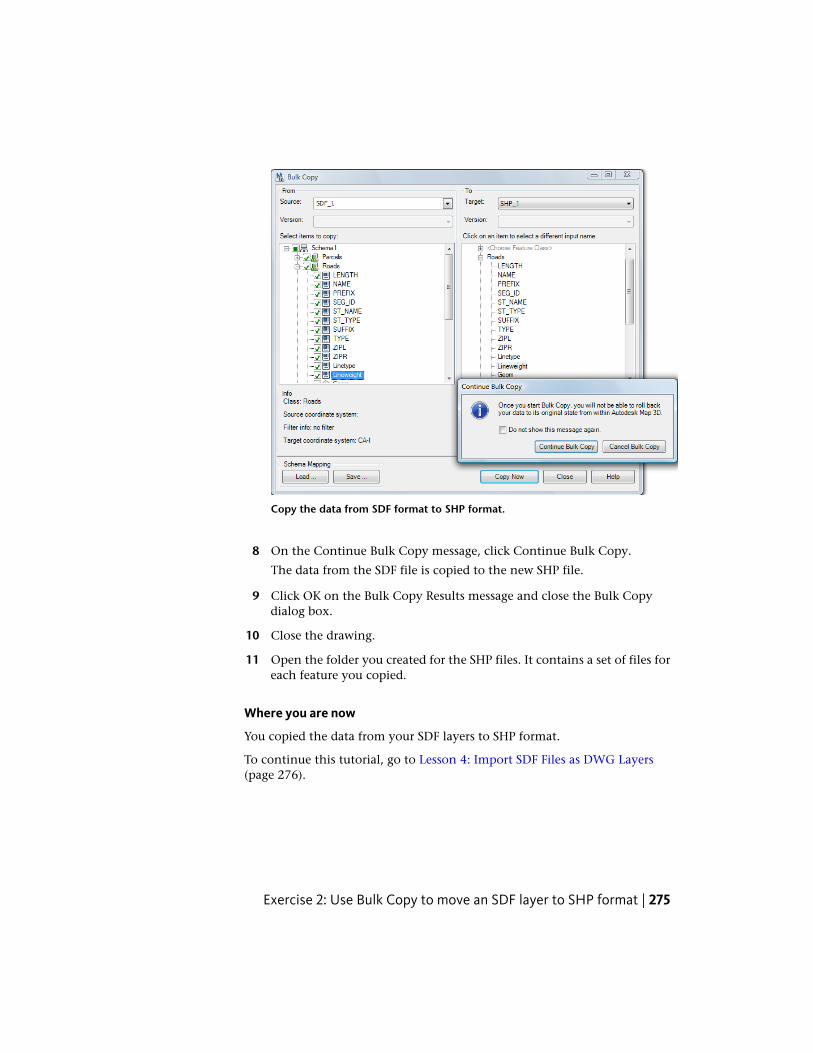
Copy the data from SDF format to SHP format.
8 On the Continue Bulk Copy message, click Continue Bulk Copy.
The data from the SDF file is copied to the new SHP file.
9 Click OK on the Bulk Copy Results message and close the Bulk Copydialog box.
10 Close the drawing.
11 Open the folder you created for the SHP files. It contains a set of files foreach feature you copied.
Where you are now
You copied the data from your SDF layers to SHP format.
To continue this tutorial, go to Lesson 4: Import SDF Files as DWG Layers(page 276).
Exercise 2: Use Bulk Copy to move an SDF layer to SHP format | 275
Lesson 4: Import SDF Files as DWG LayersYou moved some DWG data to SDF format and from there to SHP format, soyou can distribute it to people who use geospatial data.
You can move the data back into DWG format as needed. For example, ifother people change the data, you can reimport it so you have the latestversion. When you import SHP or SDF files, data is added to your map asdrawing objects, not as geospatial data.
Exercise 1: Create a template for the imported materialWhen you import the SDF file into a map, you convert the data to DWG objects.(If you connected to the SDF file, the objects would remain in SDF data format.)
To maintain the formatting of the original DWG objects that you exportedto SDF, create a template that duplicates that formatting.
Use the original drawing file as the basis for the template. That way, thetemplate automatically specifies the layers for the SDF feature classes.
NOTE This exercise uses the DWGMap.dwg map file you opened in Lesson 1:Convert Drawing Layers to Feature Classes (page 250).
To create a template for the imported material
1 Open the original DWG file you exported to SDF.
■ Click ➤ Open ➤ Drawing.
■ Select the sample map called DWGMap.dwg
2 Save the drawing as a template (.dwt) file. Click ➤ Save As ➤
AutoCAD Drawing Template.
Name the file DWGImportTemplate.dwt.
When prompted, enter a description of the template and leave the othersettings set to their default values.
3 In the new template file, delete all the drawing objects so that the drawingis empty.
Press Ctrl+A or use Zoom Window to select all the objects. Then pressthe Delete key.
276 | Chapter 7 Tutorial: Managing Data From Different Sources

4 Save and close the template drawing file.
5 Create a map using the DWGImportTemplate.dwt template.
■ Click ➤ New ➤ Drawing.
■ Select the DWGImportTemplate.dwt template.
■ Click Open.
You do not have to assign a coordinate system to this new map, becausethe template specifies that information.
To continue this tutorial, go to Exercise 2: Import the SDF layers (page 277)
Exercise 2: Import the SDF layersWhen you connected to the SDF file you created earlier in this tutorial, youbrought in its data as geospatial features. Each feature class was a separateDisplay Manager layer. However, in this lesson you import the SDF data asdrawing objects, and each feature class becomes a separate drawing layer.
NOTE This exercise uses the map you created with the DWGImportTemplate.dwttemplate and the SDF file you created in Lesson 1: Convert Drawing Layers toFeature Classes (page 250).
To import SDF layers
1 In the Tool-based Ribbon Workspace, click Home tab ➤ Data panel ➤ MapImport .
2 Change the Files Of Type to Autodesk SDF (*SDF).
3 Navigate to the SDF file you created, select it, and click OK.
4 In the Import dialog box, check Import Polygons As Closed Polylines.
5 Check that each Input Layer maps to the appropriate Drawing Layer.
Exercise 2: Import the SDF layers | 277

Be sure to select the correct drawing layer.
The drawing template has the original drawing layers defined. Since theselayers were the source for the feature classes you are importing, they aremapped appropriately.
6 Map the Size property to object data.
■ Click in the Data cell for Waterlines.
■ Click the button that appears.
■ In the Attribute Data dialog box, click Create Object Data.
■ For Object Data Table To Use, select Waterlines (not(Schema1_Waterlines).
■ Click Select Fields.
■ In the Object Data Mapping dialog box, select Size and, under TargetFields, enter Size in the corresponding cell.
■ Click OK to exit the three dialog boxes.
278 | Chapter 7 Tutorial: Managing Data From Different Sources
If you are asked to confirm your actions, click Yes.
7 Click Map Setup tab ➤ Map panel ➤ Zoom Drawing Extents.
You can now work with the objects as you would any DWG data.
To continue this tutorial, go to Exercise 3: Use display layers to assign objectproperties (page 279)
Exercise 3: Use display layers to assign object propertiesYou can create display layers for each drawing layer in your new drawing. Inaddition, you can create separate display layers for each waterline size. Bydisplaying a single display layer at a time, you can select the various sets ofobjects and assign the proper colors to them.
NOTE This exercise uses the map you created with the DWGImportTemplate.dwttemplate and the SDF file you modified in Exercise 2: Import the SDF layers (page277).
To use display layers to assign object properties
1 Create a display layer for the Parcels layer.
■ In the Task pane, switch to Display Manager. Click Data ➤ AddDrawing Data ➤ Query Current Drawing.
■ In the Define Query Of Current Drawing dialog box, click Property.
■ In the Property Condition dialog box, select Layer and set the Valueequal to Parcels.
■ Click OK to close each dialog box.
■ In Display Manager, select the default display layer name (CurrentDrawing Element) and change it to Parcels.
2 Repeat the procedures in step 1 to create a display layer for Roads.
Select the new display layer name (Current Drawing Element) and nameit Roads.
3 Repeat the procedures in step 1 to create a display layer for Waterlines.
Exercise 3: Use display layers to assign object properties | 279

Select the new display layer name (Current Drawing Element) and nameit Waterlines.
4 Create a display layer for waterlines whose Size property is set to Large.
■ In Display Manager, click Data ➤ Add Drawing Data ➤ QueryCurrent Drawing.
■ In the Define Query Of Current Drawing dialog box, click Data.
■ In the Data Condition dialog box, select Object Data.
■ For Tables, select Waterlines.
■ Select Size.
■ For Value, enter Large.
■ Click OK to close each dialog box.
■ In Display Manager, select the new display layer name (CurrentDrawing Element) and change it to Large Waterlines.
5 Repeat step 4 for the remaining sizes (Medium and Small).
6 Change the color of the Large Waterlines objects.
■ Turn off all the display layers except for Large Waterlines.To turn off a display layer, clear its check box.
■ Click View tab ➤ Navigate panel ➤ Zoom drop-down ➤ Extents.
■ Drag a selection box around all the objects that are displayed.
■ In the Quick Properties window, change the Color from ByLayer toRed.
■ Press Esc to deselect the objects.
7 Repeat step 6 for the Medium and Small layers. Make Medium objectsgreen and Small objects blue.
8 Turn on all the display elements to see the results.
AutoCAD users cannot see the display layers (because AutoCAD does nothave Display Manager). However, the layer and object properties arestored with the AutoCAD layers and objects, so the colors are visible.
280 | Chapter 7 Tutorial: Managing Data From Different Sources

Where you are now
You imported an SDF file as drawing objects, styling the imported drawingobjects as they appeared in the original drawing.
Exercise 3: Use display layers to assign object properties | 281

282

Tutorial: Working withPolygon Features
About the Polygon Features TutorialAutoCAD Map 3D has options that are designed for geospatial features withpolygon geometry. For example, you can do any of the following:
■ Use a special expression to find the area of a polygon feature.
■ Split a single polygon feature into two or more new features.
■ Merge two or more polygons into a single feature.
■ Create rules for assigning properties to polygon features after you split ormerge them.
In this tutorial, you connect to geospatial data for parcel polygons. You split aparcel into two uneven new parcels and assign attributes to each resulting parcelusing split/merge rules.
You join a data source to the parcels to add assessor data. You export the parcellayer to create a data store that contains the joined data as part of its nativeschema.
Connecting to the new data store, you create a property called “ValueByArea.”ValueByArea is a calculated property that represents the area of each parceldivided by the last sales price logged in the joined data store. You create a themebased on an expression that references the calculated property.
Finally, you publish your map to MapGuide, so others can view it on a website.You must have rights to a MapGuide 2009 Server, which supports the new
8
283
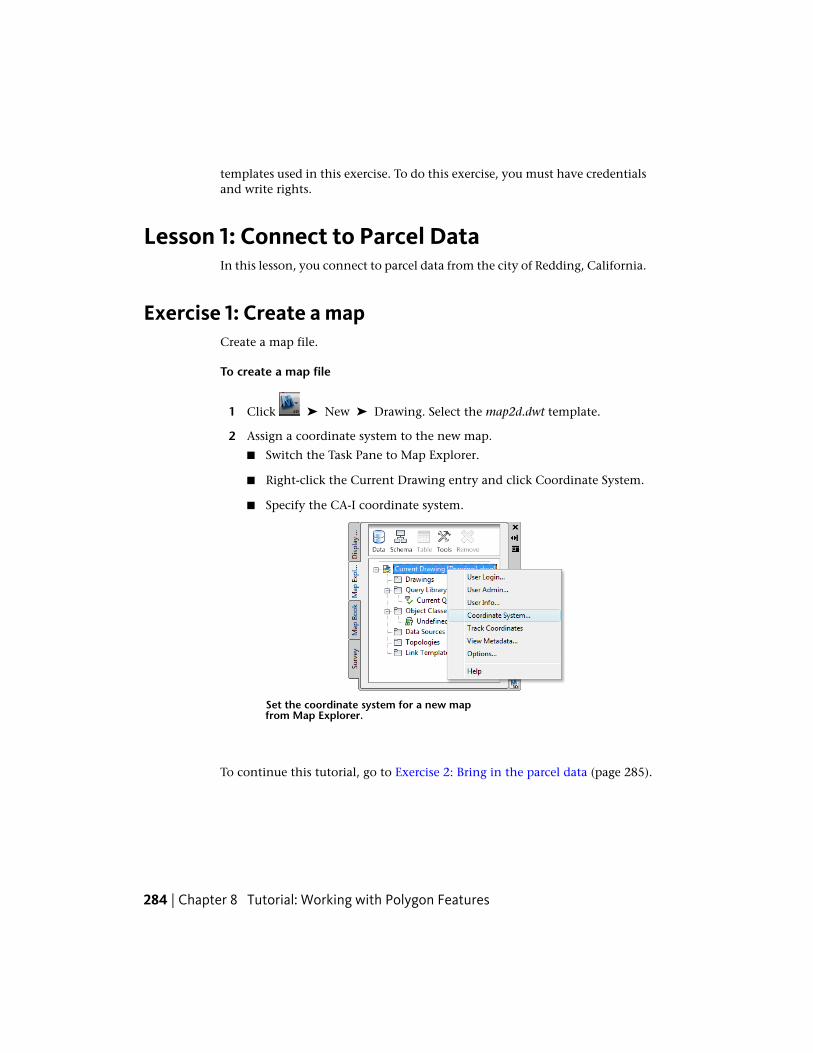
templates used in this exercise. To do this exercise, you must have credentialsand write rights.
Lesson 1: Connect to Parcel DataIn this lesson, you connect to parcel data from the city of Redding, California.
Exercise 1: Create a mapCreate a map file.
To create a map file
1 Click ➤ New ➤ Drawing. Select the map2d.dwt template.
2 Assign a coordinate system to the new map.
■ Switch the Task Pane to Map Explorer.
■ Right-click the Current Drawing entry and click Coordinate System.
■ Specify the CA-I coordinate system.
Set the coordinate system for a new mapfrom Map Explorer.
To continue this tutorial, go to Exercise 2: Bring in the parcel data (page 285).
284 | Chapter 8 Tutorial: Working with Polygon Features

Exercise 2: Bring in the parcel dataNow, add a layer that displays parcels within the city of Redding. This layercontains size, value, and address information about the parcels.
NOTE This exercise uses the map you created in Lesson 1: Connect to Parcel Data(page 284).
To add the parcel layer to the map
1 In Display Manager, click Data ➤ Connect To Data.
2 In the Data Connect window, under Data Connections By Provider, clickAdd SDF Connection.
3 Click the file icon next to the Source File field and navigate to the foldercontaining the sample files.
4 Select Assessor_Parcels.SDF and click Open.
5 In the Data Connect window, click Connect.
6 In the Data Connect window, click Add To Map.
7 Close the Data Connect window.
8 To see the data associated with this layer, select the Parcels layer in DisplayManager and click Table.
Scroll to the right to see all the columns of parcel data.
9 Leave the Data Table open for the next exercise.
Where you are now
You connected to a data store containing parcel information. You viewed thegeometry in your map and the attribute data in the Data Table.
To continue this tutorial, go to Lesson 2: Split a Polygon Feature (page 286).
Exercise 2: Bring in the parcel data | 285

Lesson 2: Split a Polygon FeatureYou can define rules that determine how properties are assigned after yousplit a single feature into multiple pieces or merge multiple features into one.In this lesson, you define split/merge rules for the Parcels feature. Then, yousplit a parcel into two uneven pieces and use the rules you defined to assignproperties to each resulting parcel.
Exercise 1: Define split/merge rulesYou can use the AutoCAD Trim and Break commands to split polygons.However, the Split command has many advantages over those methods. Asplit always results in a valid feature, and has special logic to deal withattributes automatically.
With Split, you can set rules for the assignment of properties when you splitand merge geospatial features. You can use expressions for these rules.
For example, if you are splitting a parcel, you can base the land value of theresulting parcels on a calculation that you define. You can also use automaticcalculations. For example, you can assign the average value of all mergedfeatures to the resulting feature. You can divide the value of a feature evenlyamong all its split features.
NOTE This exercise uses the map you created and modified in Exercise 1: Definesplit/merge rules (page 286).
To create split/merge rules
1 The Data Table should still be open from the last exercise. If it is not, inthe Task Pane, switch to Display Manager. Select the Parcels layer andclick Table.
2 In the Data Table, click Options (at the bottom of the window) and selectSet Split And Merge Rules.
286 | Chapter 8 Tutorial: Working with Polygon Features

Set rules for assigning properties after a split or merge operation.
Each property of the Parcels feature is listed under Feature Properties onthe left. Two properties (Geom and FeatID) are generated by the datastore, so you cannot set rules for them. If you select them, you can seethe rules that the data store uses to create them.
3 In the Split And Merge Rules dialog box, click the ADDRESS property.
4 For the Split Rule, specify Empty.
If you split this parcel, you must specify the address number for eachnew parcel that is created.
5 For the Merge Rule, specify First Selected.
If you merge multiple parcels into one, the new parcel uses the addressnumber of the first parcel you select for the merge.
6 Specify rules for other properties, using the following table as a guide.
Merge ruleSplit ruleProperty
SumProportional Based On Area2D (Geom)ACRES
First SelectedCopyAPN
SumProportional Based On Area2D (Geom)AREA
Exercise 1: Define split/merge rules | 287

Merge ruleSplit ruleProperty
SumProportional Based On Area2D (Geom)IMP_VALUE
SumProportional Based On Area2D (Geom)LAND_VALUE
SumProportional Based On Area2D (Geom)NET_VALUE
First SelectedEmptyPRIMARY_INDEX
First SelectedCopySTNAME
For a complete description of the split/merge rule options, see UsingExpressions In Split/Merge Rules.
7 Click OK.
To continue this tutorial, go to Exercise 2: Find the parcel to split (page 288).
Exercise 2: Find the parcel to splitYou can use the Data Table to find a particular parcel and zoom into it so youcan split it.
NOTE This exercise uses the map you created and modified in Exercise 1: Definesplit/merge rules (page 286).
To find the parcel to split
1 If the Data Table is not open, click the Parcels layer in Display Managerand click Table.
2 In the Data Table window, make sure Auto-Zoom is on.
When Auto-Zoom is on, it is a different color than the window
background . When it is off, it is the same color as the windowbackground.
3 Click Search To Select (at the bottom of the window).
4 In the Search To Select window, click Property and select STNAME.
5 Click = (the equals sign in the toolstrip).
288 | Chapter 8 Tutorial: Working with Polygon Features

6 Place your cursor over the text that says “value.”
7 In the tooltip that displays, click Get Values From A List.
8 Click the green arrow next to STNAME in the properties list to see thestreet names for the Parcels feature.
The properties list is populated when you click the green arrow. Your selection replacesthe selected value.
9 Click Antigua Drive and click Insert Value.
Click Next if you do not see Antigua in the list.
10 Click Validate (at the bottom of the window) to make sure that theexpression is valid.
11 When you see “The expression is valid,” click OK.
12 Click the heading for the STNAME column to sort the parcel records bystreet name.
In the Data Table, the entries for parcels on Antigua Drive are highlighted.The map is zoomed to that street, and the parcels are selected in the mapas well.
To continue this tutorial, go to Exercise 3: Split the parcel (page 290).
Exercise 2: Find the parcel to split | 289
Exercise 3: Split the parcelYou interactively divide a parcel into two unequal closed polylines.
NOTE This exercise uses the map you created and modified in Exercise 2: Findthe parcel to split (page 288).
To divide one parcel into two new parcels
1 In the Data Table, click the leftmost column for one parcel on AntiguaDrive.
Make a note of the address, so you can compare your results later.
When you click the leftmost column, you select that entry in the DataTable and automatically zoom to that parcel in your map.
2 Hide the Data Table so you can see the parcel more easily. On the Data
Table title bar, click (Auto-Hide) .
3 Click Feature Edit tab ➤ Split/Merge panel ➤ Split Feature.
4 When notified that the feature has been checked out, click Close.
5 At the first prompt, “Create new or multipart,” click New.
New splits this parcel in two pieces. You can create more pieces byselecting Multipart.
NOTE You can specify the default values for two of these prompts in theFeature Editing Options dialog box. You can turn off the prompts and alwaysuse the default values. In that case, you see only the third prompt and notthe first two.
6 At the second prompt, “Generate new feature ID or use existing,” clickNew.
This option auto-generates a unique identifier for the new parcel.
7 At the third prompt, “Would you like to draw or select the line for thesplit,” click Draw.
8 Draw the line for the parcel split and press Enter.
290 | Chapter 8 Tutorial: Working with Polygon Features
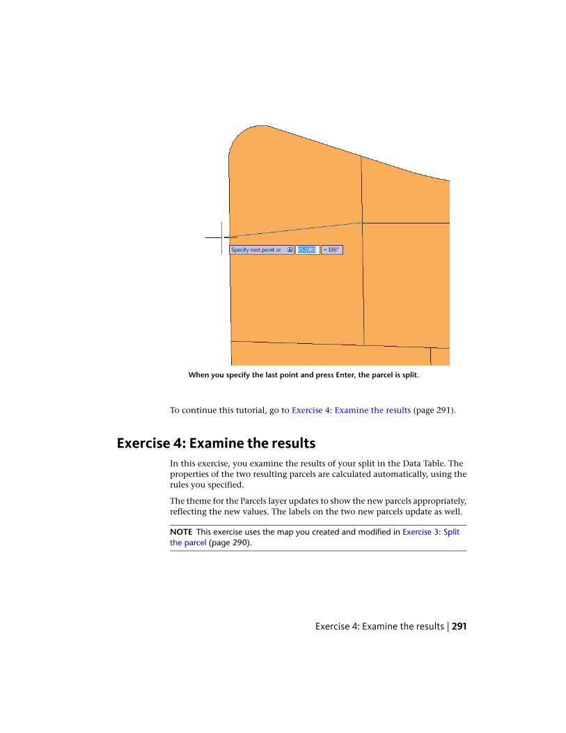
When you specify the last point and press Enter, the parcel is split.
To continue this tutorial, go to Exercise 4: Examine the results (page 291).
Exercise 4: Examine the resultsIn this exercise, you examine the results of your split in the Data Table. Theproperties of the two resulting parcels are calculated automatically, using therules you specified.
The theme for the Parcels layer updates to show the new parcels appropriately,reflecting the new values. The labels on the two new parcels update as well.
NOTE This exercise uses the map you created and modified in Exercise 3: Splitthe parcel (page 290).
Exercise 4: Examine the results | 291
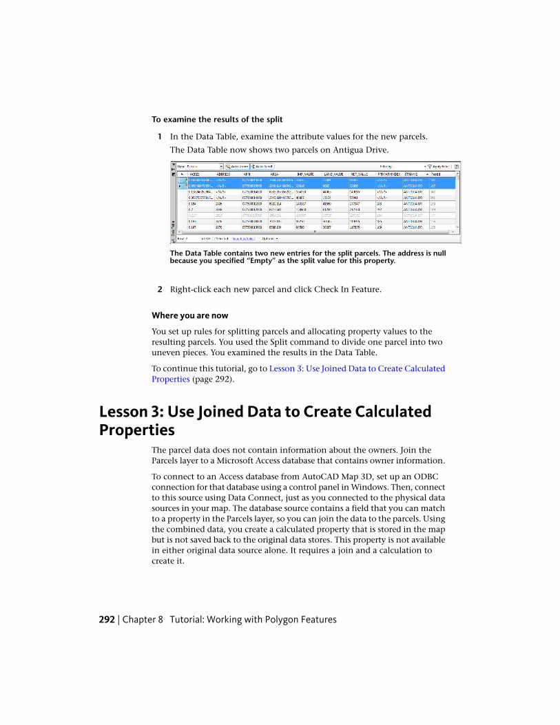
To examine the results of the split
1 In the Data Table, examine the attribute values for the new parcels.
The Data Table now shows two parcels on Antigua Drive.
The Data Table contains two new entries for the split parcels. The address is nullbecause you specified “Empty” as the split value for this property.
2 Right-click each new parcel and click Check In Feature.
Where you are now
You set up rules for splitting parcels and allocating property values to theresulting parcels. You used the Split command to divide one parcel into twouneven pieces. You examined the results in the Data Table.
To continue this tutorial, go to Lesson 3: Use Joined Data to Create CalculatedProperties (page 292).
Lesson 3: Use Joined Data to Create CalculatedProperties
The parcel data does not contain information about the owners. Join theParcels layer to a Microsoft Access database that contains owner information.
To connect to an Access database from AutoCAD Map 3D, set up an ODBCconnection for that database using a control panel in Windows. Then, connectto this source using Data Connect, just as you connected to the physical datasources in your map. The database source contains a field that you can matchto a property in the Parcels layer, so you can join the data to the parcels. Usingthe combined data, you create a calculated property that is stored in the mapbut is not saved back to the original data stores. This property is not availablein either original data source alone. It requires a join and a calculation tocreate it.
292 | Chapter 8 Tutorial: Working with Polygon Features

Exercise 1: Set up an ODBC connection for a MicrosoftAccess database
Set up an ODBC connection for the Microsoft Access database using theAdministrative Tools control panel in Windows.
NOTE If you created an ODBC connection in the tutorial, “Analyzing Data UsingStyles, Joins, and Buffers,” (page 201) you do not need to do so again. You canskip to the next exercise.
To set up an ODBC connection for the Access database
1 From your Windows desktop, click Start ➤ Settings ➤ Control Paneland open the Administrative Tools control panel.
2 In the Administrative Tools window, double-click Data Sources (ODBC).
3 In the ODBC Data Source Administrator dialog box, click Add.
4 In the Create New Data Source dialog box, click Microsoft Access Driver(*.mdb) and click Finish.
5 In the ODBC Microsoft Access Setup dialog box, for Data Source Name,enter Parcel_Owners.
6 Enter a description, for example, “Parcel owner information.”
7 Under Database, click Select.
8 In the Select Database dialog box, navigate to the sample files and selectthe Assessor.mdb file.
Specify the database for this data source.
Exercise 1: Set up an ODBC connection for a Microsoft Access database | 293
9 Click OK in the Select Database, ODBC Microsoft Access Setup, and ODBCData Source Administrator dialog boxes.
10 Close the Administrative Tools control panel.
To continue this tutorial, go to Exercise 2: Connect to the Microsoft Accessdatabase (page 294).
Exercise 2: Connect to the Microsoft Access databaseSpecify the new connection in the Data Connect window. Do not add anyspecific feature class layers from the ODBC source to the map. All theinformation becomes available to AutoCAD Map 3D automatically when youconnect to the ODBC source.
NOTE This exercise uses the ODBC source you created in Exercise 1: Set up anODBC connection for a Microsoft Access database (page 293) and the map youcreated in Lesson 1: Connect to Parcel Data (page 284).
To connect to the Access database from AutoCAD Map 3D
1 In Display Manager in AutoCAD Map 3D, click Data ➤ Connect ToData.
2 Under Data Connections By Provider, click Add ODBC Connection.
3 Click next to the Source field under Add A New Connection.
4 Select Parcel_Owners from the list of Data Source Names and click Select.
294 | Chapter 8 Tutorial: Working with Polygon Features
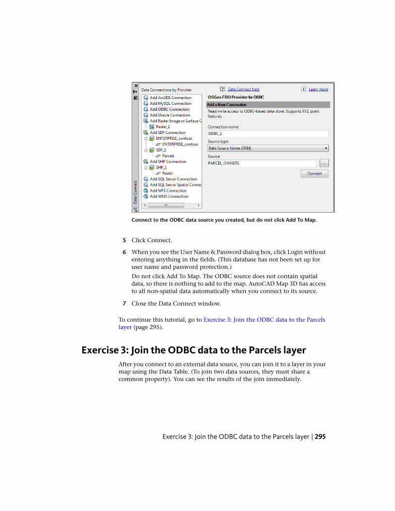
Connect to the ODBC data source you created, but do not click Add To Map.
5 Click Connect.
6 When you see the User Name & Password dialog box, click Login withoutentering anything in the fields. (This database has not been set up foruser name and password protection.)
Do not click Add To Map. The ODBC source does not contain spatialdata, so there is nothing to add to the map. AutoCAD Map 3D has accessto all non-spatial data automatically when you connect to its source.
7 Close the Data Connect window.
To continue this tutorial, go to Exercise 3: Join the ODBC data to the Parcelslayer (page 295).
Exercise 3: Join the ODBC data to the Parcels layerAfter you connect to an external data source, you can join it to a layer in yourmap using the Data Table. (To join two data sources, they must share acommon property). You can see the results of the join immediately.
Exercise 3: Join the ODBC data to the Parcels layer | 295

NOTE This exercise uses the map you modified in Exercise 2: Connect to theMicrosoft Access database (page 294).
To join the ODBC parcel data to the geospatial parcel layer
1 In Display Manager, select the Parcels layer and click Table.
2 At the bottom of the Data Table, click Options ➤ Create A Join.
3 In the Create A Join dialog box, the Primary Table Initiating The Joinentry reads SDF_1:Schema1:Parcels. For Table (Or Feature Class) To JoinTo, select the ODBC_1:Fdo:Assessor layer.
4 For This Column From The Left Table, select APN.
5 For Matches This Column From The Right Table, select APN (if it is notselected automatically).
Leave the other settings with their current values.
6 Click OK to display the original and joined data in the Data Table.
7 Scroll to the right to see the owner information.
NOTE The joined data values for the new parcel you created with the Splitcommand are not accurate. The database that contains the joined data doesnot know about the change to the parcel, so it cannot provide the propernew data for it. Update the original data store independently to enter thedata for the split parcels.
To continue this tutorial, go to Exercise 4: Save the properties to a new datastore (page 296).
Exercise 4: Save the properties to a new data storeThe Parcels layer now displays joined data. However, the joined data in theData Table is gray. The gray text reflects the fact that the joined data is notpart of the original data store. You cannot edit it or use it in a calculatedproperty.
You can save the layer out to a new data store, which will make the joinedproperties available as native properties in the future.
296 | Chapter 8 Tutorial: Working with Polygon Features

NOTE This exercise saves the layer as an SDF data store. You can use Bulk Copyto save joined and calculated properties to other geospatial data formats. For moreinformation, see Migrating GIS Data (Bulk Copy)
NOTE This exercise uses the map you modified in Exercise 3: Join the ODBC datato the Parcels layer (page 295).
To save the original and joined properties to a new data store
1 In Display Manager, right-click the Parcels layer and click Export LayerData To SDF.
Save the layer to a new SDF file to make the joinedattributes available for editing.
2 Specify a location and name for the SDF file and click Save.
3 Create a map.
■ Click ➤ New ➤ Drawing.
■ Select the map2d.dwt template.
Exercise 4: Save the properties to a new data store | 297
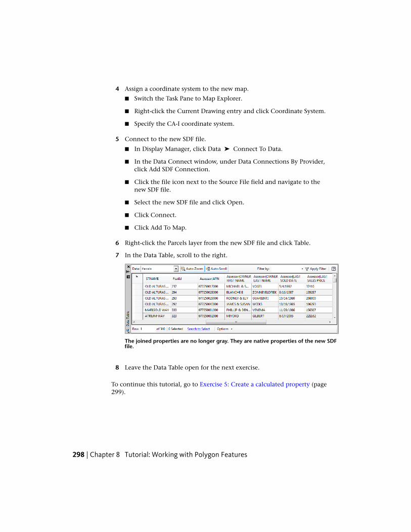
4 Assign a coordinate system to the new map.
■ Switch the Task Pane to Map Explorer.
■ Right-click the Current Drawing entry and click Coordinate System.
■ Specify the CA-I coordinate system.
5 Connect to the new SDF file.
■ In Display Manager, click Data ➤ Connect To Data.
■ In the Data Connect window, under Data Connections By Provider,click Add SDF Connection.
■ Click the file icon next to the Source File field and navigate to thenew SDF file.
■ Select the new SDF file and click Open.
■ Click Connect.
■ Click Add To Map.
6 Right-click the Parcels layer from the new SDF file and click Table.
7 In the Data Table, scroll to the right.
The joined properties are no longer gray. They are native properties of the new SDFfile.
8 Leave the Data Table open for the next exercise.
To continue this tutorial, go to Exercise 5: Create a calculated property (page299).
298 | Chapter 8 Tutorial: Working with Polygon Features

Exercise 5: Create a calculated propertyNow you have joined owner data to the Parcels layer and saved the result toa new data store. You can use the combined information to create a calculatedproperty. The calculated property is the result of an expression: in this case,the last sales price divided by the area.
NOTE To create or manage calculations, you must be connected to the data storethat contains the data for the calculation.
NOTE This exercise uses the map you modified in Exercise 4: Save the propertiesto a new data store (page 296).
To create a calculated property using joined data
1 If the Data Table is not still open from the previous exercise, select theParcels layer in Display Manager and click Table.
2 At the bottom of the Data Table, click Options ➤ Create A Calculation.
3 In the Create A Calculation dialog box, name the calculated property“ValueByArea.”
4 Click Properties. Select Assessor| LAST SALES PRICE.
Exercise 5: Create a calculated property | 299

All properties for this feature class are listed in the Propertylist.
5 Click the operator for “divided by” (the slash character).
6 Click Geometric ➤ Area2D.
This option calculates the area of a polygon.
300 | Chapter 8 Tutorial: Working with Polygon Features

7 Hold your cursor inside the parentheses, where you see the text “geometryproperty.” On the tooltip that displays, click Enter A Property.
8 From the Properties list, select Geom (at the bottom of the list).
Every spatial feature has a geometry property that you can use to calculatearea or length.
9 Click Validate to make sure that the expression is a valid calculation.
10 When you see “The expression is valid,” click OK to create the calculatedproperty and return to the Data Table.
Scroll to the right in the Data Table to see the new field. It is gray, toindicate that it is a calculated property and cannot be edited.
11 Close the Data Table.
Where you are now
You joined information from a Microsoft Access database to a layer containingparcels. You saved the layer out to a new SDF file, making all its data availablein the future. You used the new data source to create a calculated property.
To continue this tutorial, go to Lesson 4: Theme Polygon Features (page 301).
Lesson 4: Theme Polygon FeaturesYou can use the new calculated property you created as the basis for a themethat styles parcels according to their value by area.
Exercise 1: Create a themeA theme varies the display of individual features based on data values. Forexample, if you theme by parcel value, less expensive parcels can be a lightercolor while more expensive ones are a darker shade.
In this exercise, you create a theme based on the calculated property youdefined for ValueByArea.
NOTE This exercise uses the map you modified in Lesson 3: Use Joined Data toCreate Calculated Properties (page 292).
Lesson 4: Theme Polygon Features | 301

To create a theme using a calculated property
1 In Display Manager, select the Parcels layer and click Style.
2 In the Style Editor, click New Theme.
3 In the Theme Polygons dialog box, for Property, select ValueByArea.
4 For Distribution, select Jenks (Natural Breaks).
The Jenks distribution method groups ranges of features at their naturalbreaks so that features with similar values are grouped. This methodshows the natural groupings in the data, rather than creating arbitrarybreaking points.
5 Under Theme The Polygons, click next to Style Range and set theforeground color range to any two colors.
The Style Range is a gradient between two colorsyou specify.
6 Click OK twice to return to the Style Editor.
Leave the Style Editor open for the next exercise.
302 | Chapter 8 Tutorial: Working with Polygon Features
To continue this tutorial, go to Exercise 2: Add labels that use an expression(page 303).
Exercise 2: Add labels that use an expressionYou can label each parcel with text that is determined by an expression. Inthis exercise, you create a label for each parcel that displays the parcel addresson two lines.
The Style Editor should still be open from the previous exercise.
NOTE This exercise uses the map you modified in Exercise 1: Create a theme(page 301).
To add labels using expressions
1 In the Style Editor, click the entry under Feature Label for the first rulein the theme.
Because you are theming the Parcels feature, you have one entry for eachtheme rule.
2 In the Style Label dialog box, click Property To Display, scroll down tothe bottom of the list, and click Expression.
Exercise 2: Add labels that use an expression | 303
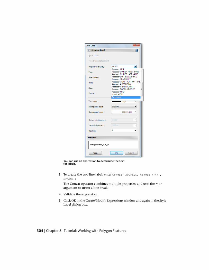
You can use an expression to determine the textfor labels.
3 To create the two-line label, enter Concat (ADDRESS, Concat ('\n',
STNAME))
The Concat operator combines multiple properties and uses the '\n'argument to insert a line break.
4 Validate the expression.
5 Click OK in the Create/Modify Expressions window and again in the StyleLabel dialog box.
304 | Chapter 8 Tutorial: Working with Polygon Features
6 In the Style Editor, click the entry under Feature Label for the second rulein the theme.
7 In the Style Label dialog box, click Property To Display, scroll down tothe bottom of the list, and click the Concat expression you created earlier.Click OK twice.
Once you create an expression for a label, you can select it from theProperty To Display list. You do not have to re-create it each time.
8 Repeat steps 5 and 6 for each entry in the theme for which you wantlabels.
9 Close the Style Editor to see the changes.
Where you are now
You themed the Parcels layer, using a calculated property as the basis for thetheme. You added labels whose content was determined by an expression.
To continue this tutorial, go to Lesson 5: Publish Your Styled Map to MapGuide(page 305).
Lesson 5: Publish Your Styled Map to MapGuideWhen you publish a styled map to MapGuide, all queries, filters, labels, andcalculated properties are saved to a .layer file and transferred to MapGuide.
From within AutoCAD Map 3D, you can preview the published informationjust as it will appear on the website.
You must have rights to a MapGuide 2009 Server, which supports the newtemplates used in this exercise. To do this exercise, you must have credentialsand write rights.
Exercise 1: Publish to MapGuideWhen you publish to Autodesk MapGuide, you create a web page containinga picture of your map. You must have rights to a MapGuide 2009 Server, whichsupports the new templates used in this exercise. To do this exercise, you musthave credentials and write rights.
NOTE This exercise uses the map you modified in Lesson 4: Theme PolygonFeatures (page 301).
Lesson 5: Publish Your Styled Map to MapGuide | 305
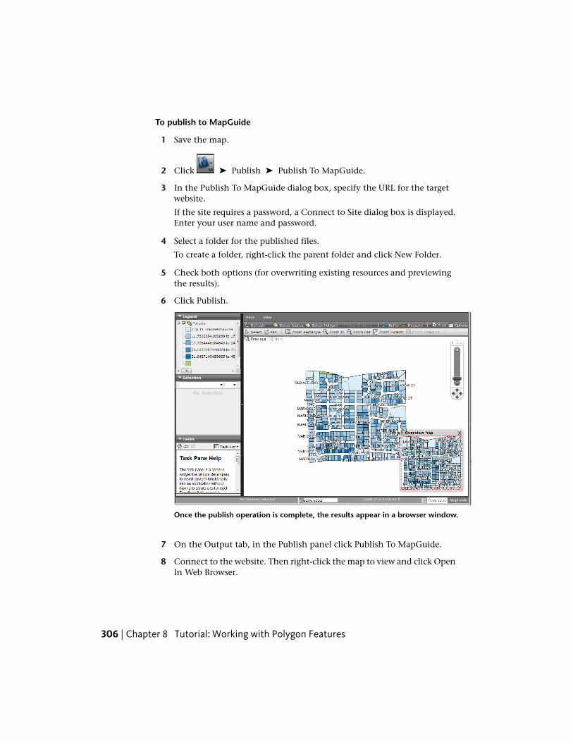
To publish to MapGuide
1 Save the map.
2 Click ➤ Publish ➤ Publish To MapGuide.
3 In the Publish To MapGuide dialog box, specify the URL for the targetwebsite.
If the site requires a password, a Connect to Site dialog box is displayed.Enter your user name and password.
4 Select a folder for the published files.
To create a folder, right-click the parent folder and click New Folder.
5 Check both options (for overwriting existing resources and previewingthe results).
6 Click Publish.
Once the publish operation is complete, the results appear in a browser window.
7 On the Output tab, in the Publish panel click Publish To MapGuide.
8 Connect to the website. Then right-click the map to view and click OpenIn Web Browser.
306 | Chapter 8 Tutorial: Working with Polygon Features
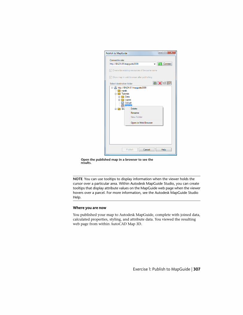
Open the published map in a browser to see theresults.
NOTE You can use tooltips to display information when the viewer holds thecursor over a particular area. Within Autodesk MapGuide Studio, you can createtooltips that display attribute values on the MapGuide web page when the viewerhovers over a parcel. For more information, see the Autodesk MapGuide StudioHelp.
Where you are now
You published your map to Autodesk MapGuide, complete with joined data,calculated properties, styling, and attribute data. You viewed the resultingweb page from within AutoCAD Map 3D.
Exercise 1: Publish to MapGuide | 307

308
Glossary
AcDbEntity A standard AutoCAD object, such as a line or arc, that can have properties suchas color, linetype, or lineweight.
adjacent arrows Polygonal objects in a map book template that display the map tilesimmediately contiguous to the current one.
attribute data Tabular data that describes the characteristics of a feature (page 311), for example,the number of lanes and pavement-type belonging to a road feature. See also external data(page 311), object data (page 313), property (page 313).
AutoCAD layer A logical grouping of data. Layers are like transparent acetate overlays on adrawing. An AutoCAD layer differs from a map layer in Display Manager (page 310). A DisplayManager layer references a feature source or a drawing source, contains styling and theminginformation, and optionally has a collection of scale ranges. See also layer (page 312), drawinglayer (page 311), feature layer (page 311), or surface layer (page 315).
Autodesk Design Review A free software utility that allows anyone to view, print, measure,mark up, and revise 2D and 3D designs created by Autodesk design software. You do not needthe original design-creation software to use this tool.
buffer A zone of a specific radius created around a selected feature. Used to select featureswithin a specific distance of another feature. In AutoCAD Map 3D, you can define buffers fordrawing topologies and for features, but you define them differently.
COGO Short for Coordinate Geometry. COGO inquiry commands extract geometricinformation from drawing objects such as lines, curves, closed polylines, and polygons. UseCOGO input commands to enter accurate geometry when creating objects. For example, youcan create parcel boundaries from legal documents or survey data.
Enter COGO commands from a dialog box or “transparently.” Use transparent COGOcommands by entering an apostrophe ( ' ) before the command name.
constrained Restricted to particular values. A feature class property that is constrained isvalidated when a new feature is added to that class. For example, a "minor road" feature classmay be constrained to be 25, 30, or 40 miles per hour.
9
309

contour lines A line that connects points of the same elevation or value relative to aspecified reference datum. The lines can help you determine the elevation at a specificlocation on a surface. They help clarify and analyze the 3D surface terrain, and help withtasks such as navigation.
coordinate system See global coordinate system (page 312).
Create Method A setting on the Class Settings tab of the Define Object Classification dialogbox. It determines the method used to create new objects from this class (when you right-clickthe object class and choose Create Classified Object).
Data Connect AutoCAD Map 3D window where you can access a data store (page 310) andadd specific data to your map. Display the Data Connect window by clicking Data in MapExplorer (page 312) or Display Manager (page 310) (in the Task Pane (page 315)).
data provider Used by Data Connect to connect to geospatial data store (page 310)s.
data store A collection of feature class (page 311)es contained in a single data storage location.The data store contains feature classes defined within one or more schemas. Data stores canbe files, such as an SDF file, or databases, such as an Oracle Spatial database.
Data Table In AutoCAD Map 3D, the feature (page 311)-based grid where you can view andedit attributes of selected spatial features, perform searches, and work with selection sets.
DEM Digital Elevation Model. A file that contains a representation of surface terrain. Thesurface is stored as a grid. Each grid cell can have any one of several different meanings,such as elevation, color, density, and so on.
digitize To convert existing data from paper maps, aerial photos, or raster (page 314) imagesinto digital form by tracing the maps on a digitizer. Object locations are recorded as X,Ycoordinates.
Display Manager A tab in the Task Pane (page 315) that handles the styling and theming offeature (page 311)s in your map.
display map All the settings for a specific map, such as the data to include, the appearanceof each layer (page 312), and the legend definition. A display map can include objects fromattached drawings, raster (page 314) images, and feature (page 311)s stored in data store (page310)s. For example, it can include data from Oracle databases, SDF or SHP files, and ArcSDE.One map can include multiple display maps.
draping The process of displaying a set of features or a raster (page 314) image on a surfaceso that the features or the image reflect the underlying terrain.
Draw Query A query that retrieves objects (copies them into the current drawing). You canmanipulate and edit the objects. You can save them back to their attached drawings, savethem to the current drawing, or save them to a new drawing.
310 | Chapter 9 Glossary
drawing layer A layer in Display Manager (page 310) that contains drawing objects from aDWG file. See also AutoCAD layer (page 309), feature layer (page 311), layer (page 312), or surfacelayer (page 315).
drawing set The set of source drawing (page 315)s attached to a map.
drawing source In AutoCAD Map 3D, a drawing (DWG) file and also its associatedinformation, such as attached drawing files, drawing-based feature class (page 311)es, linkedtemplate data, and topologies. Compare with feature source (page 311).
drive alias In AutoCAD Map 3D, the mechanism that points to the folder where attachedDWG files are stored.
DWF Design Web Format. An Autodesk file format for sharing two-dimensional,three-dimensional, and spatially enabled design data on the Web.
external data The attribute data (page 309) linked to a map object but contained in a databaseor file outside the map file. See also object data (page 313), property (page 313).
FDO Feature Data Objects data access technology. An Autodesk software standard andgeneral purpose API for accessing feature (page 311)s and geospatial data regardless of theunderlying data store (page 310). See also feature class (page 311).
feature An abstraction of a natural or man-made real world object. A spatial feature has oneor more geometric properties. For example, you can represent a road feature with a line,and a hydrant with a point. A non-spatial feature does not have geometry, but can be relatedto a spatial feature that does. For example, a road feature can contain a sidewalk featurethat is defined as not containing any geometry. See also attribute data (page 309), FDO (page311).
feature class A schema element that describes a type of real-world object. It includes a classname and property (page 313) definitions. Commonly used to refer to a set of feature (page311)s of a particular class, for example, the feature class "roads" or the feature class "hydrants."See also FDO (page 311), schema (page 314).
feature layer A layer in Display Manager (page 310) containing feature (page 311)s from asingle feature class (page 311) in a spatial data source. Feature layers are added to your mapusing Data Connect. See also AutoCAD layer (page 309), drawing layer (page 311), layer (page312), or surface layer (page 315).
feature source Any source of feature (page 311) data that has been connected to a map.Compare with drawing source (page 311).
field A specific category of information in a data file, such as Address or Diameter.
geometry (Oracle Spatial database) The representation of a spatial feature (page 311).
| 311
GIS (Geographic Information System) A computerized decision support system thatintegrates geographic data, attribute data (page 309), and other spatially referenced data. AGIS is used to capture, store, retrieve, analyze, and display spatial data (page 315).
global coordinate system A method that converts the coordinates representing latitudeand longitude into an AutoCAD Map 3D map Cartesian coordinate system. This methodaccounts for the curvature of the surface of the earth with a projection. A coordinate systemcan use a projection, an ellipsoid definition, a datum definition, standard parallels, and acentral meridian to define it.
inset A detailed, large-scale portion of a map, often placed on the same sheet as asmaller-scale map of the larger area.
join A relationship that is established between attribute data and feature sources to createa view of the combined data for ad-hoc analysis.
key view A thumbnail view of an entire map. You can create a simplified view of the mappedarea to use as the key view.
label Text placed on or near a map feature (page 311) that describes or identifies it.
layer A resource that references a feature class (page 311) or a drawing source (page 311) thatyou add using Display Manager (page 310). The layer contains styling and theminginformation, and optionally a collection of scale ranges. See also AutoCAD layer (page 309),drawing layer (page 311), feature layer (page 311), or surface layer (page 315).
legend A table that lists the styles in your map and specifies which layers or map scalesthey represent.
lock To make all or part of a disk file read only so that other users on a network cannotmodify it. Object locking applies to objects that another user is editing. File locking appliesto entire files, for example when an AutoCAD user wants to open a file while the file is beingedited in AutoCAD Map 3D.
logical operator A symbol such as And, Or, Not, =, >, >=, <, and <= used to define logicalrelationships.
map A collection of layers displayed within a consistent coordinate system and extents. Seealso layer (page 312).
map book A collection of map tiles that you publish as separate pages. You can specify thelayout and properties for your map book on the Map Book tab of the Task Pane (page 315).
Map Explorer The Task Pane (page 315) tab where you manage your mapping resources.
312 | Chapter 9 Glossary
map query A set of conditions that specify the selection of drawing objects from sourcedrawing (page 315)s. These conditions can be based on the location or properties of an objector on data stored in the drawing or in a linked database table.
metadata Data about data. In the GIS context, metadata consists of information thatdescribes the essential characteristics of geospatial data sets.
Mpolygon A polygon object. A polygon differs from a closed polyline in that it storesinformation about its inner and outer boundaries.
north arrow A visual indicator of the northern direction in a map. Sample north arrowsand scale bars (both metric and imperial) are available as dynamic blocks for you to insertinto your maps.
object class All the drawing objects that have been created using a specific object classdefinition. Use object classification to organize objects in your drawing based on thereal-world features they represent, such as roads. Object classes allow you to create newobjects that automatically have the appropriate properties and values for objects in yourdrawing.
object class definition How to create a classified drawing object in a drawing. An objectclass definition can include information about the object type, default properties of theobject, or default data to attach to the object.
object data The attribute data (page 309) attached to a drawing object and stored in thedrawing file. Compare with external data (page 311).
Object Type (drawing classification) A setting on the Applies To tab of the Define ObjectClassification dialog box that determines which existing objects you can add to this objectclass. If the object was not created with the selected method, you cannot add it.
overlay analysis Provides spatial and data analysis capabilities for two sets of geospatialfeatures. Use an Overlay operation to compare two layers that overlap in space.
polygon A closed area that stores information about its inner and outer boundaries, andabout other polygons nested in it or grouped with it. In a polygon topology, any lines orarcs in the drawing can enclose the polygon. In addition, AutoCAD Map 3D supports apolygon object, sometimes called an Mpolygon (page 313) or mapping polygon.
Preview Query A query that displays the objects on screen, but does not retrieve them.When you change the screen, the objects disappear.
property A single attribute of a feature class (page 311). A feature class has one or moreproperty definitions. For example, you can have a Road feature class with properties calledName, NumberLanes, or Location. See also attribute data (page 309), feature (page 311).
publish To generate output from a map.
| 313

query A set of criteria for specifying the selection of objects or records. For example, a layer(page 312)-based query can display only the objects on the layers that contain state anddistrict boundaries.
raster Images containing individual dots (called pixels or cells) with color values, arrangedin a rectangular, evenly spaced array. Aerial photographs and satellite images are examplesof raster images used in mapping. Compare with vector (page 316).
resolution In a raster (page 314) image, the density of pixels-per-inch (PPI) or dots-per-inch(DPI).
save set Objects that were created or modified in the current drawing and are marked to besaved back to source drawing (page 315)s.
scale The ratio of the distance on a paper map to the distance on the ground. A scale of1:100,000 (also represented as 1/100000), means that a distance of one unit on the mapcorresponds to 100,000 units on the ground. On a digital map, scale represents the scale ofthe map from which the digital map was derived.
scale threshold Levels at which a map display changes. You can define different style (page315)s at different scale thresholds. For example, turn on the display of road names only whenthe drawing scale factor is below 1:5000.
schema The metadata that provides a logical description of multiple feature class (page 311)esand the relationships between them.
SDF Spatial Data File. The current version of the SDF format that is the native format forthe Autodesk MapGuide technology (Autodesk MapGuide Enterprise 2007 and MapGuideOpen Source). Each SDF file can contain multiple feature class (page 311)es or types of datastored in tables with attributes and geometry.
SDF 2 A previous version of the SDF file format that was the native file format for AutodeskMapGuide (the last release was Autodesk MapGuide 6.5). Each SDF 2 file generally containedone feature (page 311) or type of data, for example points, lines, polygons, or text.
sheet An individual named object in a sheet set (page 314) that can be published. A sheetreferences a layout.
sheet set A named collection of sheets and sheet subset (page 314)s for publishing.
sheet subset A named collection of sheets within a sheet set (page 314). An individual sheetcan be a member of only a single subset.
sheet template A drawing file that defines a title block and a layout for use in sheets. Asheet template can be specified for sheet set (page 314)s and sheet subset (page 314)s.
314 | Chapter 9 Glossary

source drawing A drawing file attached to another drawing. The set of all source drawingsattached to a drawing is called the drawing set. Use a query to retrieve selected objects frommultiple source drawings.
spatial A generic term used to reference the mathematical concept of n-dimensional data.
spatial data Information about the location and shape of geographic feature (page 311)s,and the relationships between those features.
spatial database A database containing information indexed by location.
style Settings that specify how to display the objects in a Display Manager (page 310) layer.For example, you can style color, linetype, linewidth, and scale.
SuperUser An AutoCAD Map 3D user who can perform user administration tasks, set systemoptions, and perform any other AutoCAD Map 3D operation.
surface layer A layer in Display Manager (page 310) containing feature (page 311)s from araster (page 314) image that contains elevation information. Surface layers are added to yourmap using Data Connect. See also See also AutoCAD layer (page 309), drawing layer (page 311),feature layer (page 311).
Survey A tab on the Task Pane that allows you to bring in LandXML or ASCII point data,manage the resulting point layer, and Bulk Copy the data to another data store.
table A set of data arranged in records (rows) and fields (columns). When a table is displayedin a grid, records are displayed in horizontal rows and fields are displayed in vertical columns.Each field value in the table is displayed in a cell.
Task Pane AutoCAD Map 3D window that displays information about the current drawing.The Task Pane contains four tabs: Map Explorer (page 312), Display Manager (page 310), MapBook (page 312), and Survey (page 315). You can resize the Task Pane and place it where youwant.
template A paper space layout you can use as the basis for a new layout. The paper spaceobjects and page setup in a template are used for any new layout you create with thattemplate. You can keep, delete, or modify any of the objects from a template you use. Nomodel space objects are included. Layout templates are identified with a .dwt file extension.
theme A style (page 315) that varies the appearance of an element in a layer based on thevalue of a specific property (page 313). For example, instead of coloring lakes blue, you couldvary the shade of blue based on the depth of the lake. Instead of choosing one line widthfor all roads, you could vary the line width based on number of lanes.
tile Map books divide a single map into a set of tiles and display each tile on a separate mapbook page.
| 315

title block A defined DWG block that can include title information, such as your companyor group name and the name of the map. Many organizations have standard title blocks toinsert in this element. You can define certain attributes of the title block from within yourtemplate. When you generate the map book, you can choose a drawing for the title block.That drawing replaces the original title block contents defined in the template layout.
unclassified objects Objects that have not been assigned to any object class (page 313).
user privileges The AutoCAD Map 3D operations available to each user.
vector A mathematical calculation of an object with precise direction and length. Vectordata is stored as X,Y coordinates that form points, lines, and areas. Compare with raster(page 314).
viewport (paper space) A view of model space from a layout.
Workflow An automated set of tasks that can be arranged to run in series or parallel. Theoutput of one task can be used as the input of another task. The user can configure thesequence and parameters for execution graphically.
workflow activity A single step in a workflow that executes a command or set of commands.
workflow binding A relationship between activities such that the output of one activityis used as the input of another.
workspace Contains the commands and tools for specific tasks. The Tool-Based Ribbonworkspace is tailored to those already familiar with the AutoCAD ribbon, while the Task-BasedRibbon is optimized for mapping tasks.
Click the current workspace name in the status bar (page 23)to change the workspace.
zoom To change the display magnification. Magnification focuses on progressively smallerareas of an image (when you zoom in) and larger areas (when you zoom out).
zoom extents To magnify a drawing based on its extents so that the view shows the largestpossible view of all spatial objects.
316 | Chapter 9 Glossary
Index
2Ddraping data on 3D surfaces 209
3Ddraping 2D data on 209
A
application menu 6search field 9
application windowAutoCAD Map 3D 4
attached drawingspreviewing 100
attachingdrawings to a map 99
AutoCAD drawingsassigning a drive alias 83cleaning up 89georeferencing 83preparing for AutoCAD Map 3D 83
AutoCAD layersconverting to feature classes 250importing data to 277
AutoCAD Map 3Dapplication window 4command line interface 25dynamic input 25model and layout tabs 24Properties palette 20ribbon 6ribbon workspaces 6right-click menus 28shortcut menus 28status bar 23Task Pane 12workspaces 11
AutoCAD Raster Designdigitizing paper drawings 83
AutoCAD userslearning AutoCAD Map 3D 83
preparing drawings for AutoCAD Map3D 83
Autodesk Design Review 175, 196automatic update
turning off while editing 65automating tasks (tutorial) 239, 243–244
B
background colorchanging for maps 202
background imagesplacing behind drawing objects 119
brightnessadjusting for raster images 120
buffersand points 237creating 221tutorial 220, 237using to filter data 222
Bulk Copytutorial 272
C
calculated propertiestutorial 283, 299
checking infeatures after editing 65
checking outfeatures for editing 65
classificationdrawing objects 135
classifying objectstutorial 135
cleaning updrawings 89duplicate objects 90
clippingraster images 122
Index | 317
colorsfor themes 50
command lineinterface in AutoCAD Map 3D 25
Command promptin AutoCAD Map 3D 25
commandsfinding on the ribbon 9
composite styles 56connecting
data sources using drag-and-drop 38to DWG files 39using Data Connect 43
contrastadjusting for raster images 120
coordinate systemssetting for map 38setting for maps 30setting when connecting to data 45
creatingnew features on existing layers 60
CSV files (comma-separated)exporting to from Data Table 228
D
dataexporting to CSV 228moving to different sources 247purchasing for maps 74web-based sources 75–76
Data Connectand raster images 45
Data Connect (tutorial) 43data stores
types 202Data Table
adding information for features 62displaying for layers 63exporting data from 228filtering 63updating after editing features 66using for joins 218, 295zooming to a view 63
definingobject classes (tutorial) 139
defining split/merge rules 286deleting duplicate objects 90Design Web Format
publishing to 70digital maps
purchasing 76DigitalGlobe
satellite photos 75digitizing
paper drawings with AutoCAD RasterDesign 83
dispaly orderchanging 119
Display Managerand themes 49attaching DWG files to maps 39AutoCAD Map 3D 12tab in Task Pane 16using for drag and drop 38
Display Manager layersadding raster images to 125renaming 125
drag-and-drop methodfor connecting to feature sources 38
draw queries 98Drawing Cleanup
deleting duplicates 90extending undershoots 93profiles 96tutorial 89
drawing errorscorrecting 89
drawing objectsadding to a map 98assigning to object classes
(tutorial) 148classifying (best practices) 174classifying (tutorial) 135converting to other formats 247converting to SDF 250creating with object classes
(tutorial) 159deleting duplicates 90editing with object classes
(tutorial) 159exporting to SDF 255
318 | Index
extending undershoots 93georeferencing 86importing SDF data as 276retrieving using property
queries 102drawing properties
mapping to feature classes 259drawings
attaching to a map 99drive alias
creating 83–84DSN (Data Source Name)
creating in Windows XP 215DSNs
creating for use with maps 293DWF (Design Web Format)
choosing sheets to publish 72publishing map books to
(tutorial) 196publishing options 130publishing to 70, 127setting publishing options 70
DWF filesviewing 175
DWG filesattaching to maps 39querying objects into maps 41
dynamic input 25Dynamic Input
in AutoCAD Map 3D 25
E
electric industry toolkit 136elevation
showing with styling 202exporting
and object data 128filtered layer data 224object classes (tutorial) 168
expressionstutorial 303
extending undershoots 93external data
joining to layers 215, 292
F
fadeadjusting for raster images 120
feature classescreating from AutoCAD layers 250mapping object classes to
(tutorial) 168mapping object data to 256mapping properties to 259
feature sourcesdragging and dropping 38
featuresadding data for 62automatic check-out 65checking in 65creating 60editing 65locking while editing 65updating after editing 66
filteringData Table 63
flood analysistutorial 229, 231
G
geodata portal 74georeferenced DWFs
publishing 70georeferencing drawings 83geospatial data
copying to a different format 272geospatial features
adding data for 62creating 60
I
image framesdisplaying 120
image informationviewing 117
imagesadding to maps 114
Index | 319

inserting without using DataConnect 114
importingfeature classes as AutoCAD
layers 277information
viewing for raster images 117Insert Image command
tutorial 114inserting
raster images 114insets
and map books 193Intermap
topographic images 76
J
joinsand styling 215, 219, 292tutorial 218, 295
K
key map viewsand map books 186
L
labelsadding to themes 52tutorial 303
layerscomparing 225displaying Data Table for 63exporting 224mapping imported data to AutoCAD
layers 277layouts
and publishing 72legends
and map books 186changing order of items 69creating for maps 67excluding items from 69
inserting 67lines
composite styles 56location
queries 105locking
features while editing 65
M
managing datatutorial 247
Map Book tabin Task Pane 17
map booksadding an inset 193creating with templates 186customizing north arrows 185customizing templates 178, 180customizing title blocks 182generating 189including a key map view 186including a legend 186previewing 189publishing to DWF 196saving settings 189settings for 187specifying printers or plotters
for 178templates and north arrows for 185templates and plotters for 178templates and title blocks for 182templates and viewports for 180templates for 178tutorial 175
Map BooksAutoCAD Map 3D 12
Map Classic 11Map Explorer
AutoCAD Map 3D 12Map Explorer tab 14map2d.dwt 30MapGuide
tutorial 305tutorial for publishing 283
320 | Index

mapschanging background color for 202creating (tutorial) 30
menu commandsfinding on the ribbon 9
menusin AutoCAD Map 3D 6
metadataand object classification
(tutorial) 165model and layout tabs
AutoCAD Map 3D 24multi-user editing
and drive aliases 84multiline labels
tutorial 303multiple drawings
attaching to a map 99
N
NAVTEQdigital maps 76
north arrowsfor map book templates 185
O
object classesand export(tutorial) 168and metadata(tutorial) 165assigning objects (tutorial) 148creating objects (tutorial) 159defining (tutorial) 139editing objects (tutorial) 159predefined 136using in new maps(tutorial) 153
object classificationand industry toolkits 136and new maps (tutorial) 153and SuperUser privileges 137best practices 174tutorial 135
object dataand exporting 128mapping to feature classes 256
object data indexcreating 112
ODBCconnecting to data 217joining data to features 218setting up connections 215
ODBC connectionssetting up 292–293
ODBC dataconnecting to 294
organization namechanging for map book 182
overlaysautomating (tutorial) 239tutorial 229, 231
P
plot datechanging for map books 182
plottersspecifying for map books 178
pointsstyling as symbols 77tutorial 236
polygon features 286labeling tutorial 303splitting 286splitting (tutorial) 283theming tutorial 301tutorial 283
preview queries 98previewing
attached drawings 100using property queries 102
profilescreating for Drawing Cleanup 96
propertiesadding to SDF data stores 262adding to SDF features 269
Properties paletteAutoCAD Map 3D 20
proximityusing to analyze data in maps 220
publishingto DWF 70
Index | 321
publishing optionsfor DWF 130
Q
queriescomplex 105creating an object data index
for 112for adding drawing objects to a
map 98for DWG objects 41for previewing 98location 105multiple criteria 105previewing with 102property 102using buffers with 222
queryingdrawing objects with no coordinate
system 86DWG objects into maps 41
Quick Access Toolbar 6Quick View
tutorial 98, 100
R
raster imagesadding to Display Manager
layers 125adding with Data Connect 45adjusting image brightness 120adjusting image contrast 120adjusting image fade 120clipping 122displaying behind drawing
objects 119displaying frames for 120inserting 114moving behind other layers 47viewing information for 117viewing size 117
ribbonchanging tab order 6
finding commands from previousreleases 9
in AutoCAD Map 3D 6keyboard shortcuts 6
Ribbon Command Locator 9right-click menus
AutoCAD Map 3D 28Rubber Sheet
and georeferencing 86
S
sample files for tutorials 2satellite images
choosing a transparent color in 77satellite photos
purchasing 75Schema Editor
tutorial 269schemas
editing 267SDF
converting drawing objects to 250exporting drawing objects to 255exporting layers to 224importing data as drawing
objects 276SDF files
adding properties to 262, 269dragging and dropping 38
shared drawingssetting up a drive alias for 84
sheet setschoosing for publishing 72
shortcut menusAutoCAD Map 3D 28
SHP filesconnecting to 43
split/merge rulesdefining 286
splittingpolygon features (tutorial) 283, 286
status barAutoCAD Map 3D 23
stylesand joins 219
322 | Index

and zoom levels 56, 59combining two line styles 56composite 56
stylingto show elevation 202
SuperUsersetting privileges 137
surfacesdraping vector data on 209draping vector files on 212styling to show elevation 202theming 77, 204
Survey tab 18AutoCAD Map 3D 12
symbolsusing for point features 77
T
Task PaneAutoCAD Map 3D 12Display Manager tab 16Map Book tab 17Map Explorer tab 14Survey tab 18
Task-based Ribbon workspace 11templates
for map books 178, 180, 182, 185for new maps 30object classification 136tutorial 276using to create map books 186
text stylechanging for map books 182
themesadding labels 52and map scale 52and ranges of values 49defining colors 50for surfaces 77for surfaces with elevation 204
themingtutorial 301
title blocksfor map book templates 182
Tool-based Ribbon workspace 11
topographic imagespurchasing 76
transparencyand satellite images 77and underlying surfaces 212changing for layers 47
tutorialsadding a property to an SDF file 262adding points 236applying themes to surfaces 204AutoCAD to AutoCAD Map 3D 83buffers 220, 237Bulk Copy 272calculated properties 283, 299changing map background
color 202comparing layers 225connecting to SDF files 262creating a template 276display layers 279Drawing Cleanup 89drawing queries 98editing schemas 267exporting display layers 283, 296exporting from DWG to SDF 127–
128, 255exporting to CSV 228expressions 303filtering data with buffers 222importing SDF data as drawing
objects 276joined data 283joins 215, 218, 292, 295joins and styling 219labeling polygon features 303location queries 105making layers transparent 212managing data 247map books 175mapping drawing properties to feature
class properties 259mapping object data to feature
classes 256mapping to AutoCAD layers on
import 277migrating data 247
Index | 323

multiline labels 303object classification 135ODBC connections 215, 293ODBC data sources 217, 294overlay 229, 231overview 1publishing maps to DWF 127publishing to MapGuide 283, 305raster images 114resizing the window for 3sample files for 2Schema Editor 269searching to select 288splitting polygon features 283, 286styling surfaces to show
elevation 202theming polygon features 301workflows 239workspace for 4
U
undershootsextending 93
updatingfeatures after editing 65
user rights (tutorial) 137
V
vector datadraping on 3D surfaces 209
viewportsfor map books 186resizing on templates 180
W
wastewater industry toolkit 136water industry toolkit 136workflows
editing (tutorial) 239, 243running (tutorial) 244tutorial 239
working offline 65workspaces
AutoCAD Map 3D 6selecting for tutorials 4switching between 11
Z
z-orderchanging 47
zoom levelsand styles 59assigning styles to 56
zoomingusing Data Table 63
324 | Index