Machine Vision and Applications (2013) 24:567–578DOI 10.1007/s00138-012-0417-5

ORIGINAL PAPER

A database for automatic classification of forest species

J. Martins · L. S. Oliveira · S. Nisgoski · R. Sabourin

Received: 7 June 2011 / Revised: 14 November 2011 / Accepted: 13 February 2012 / Published online: 20 March 2012© Springer-Verlag 2012

Abstract Forest species can be taxonomically divided intogroups, genera, and families. This is very important for anautomatic forest species classification system, in order toavoid possible confusion between species belonging to twodifferent groups, genera, or families. A common problemthat researchers in this field very often face is the lack ofa representative database to perform their experiments. Tothe best of our knowledge, the experiments reported in theliterature consider only small datasets containing few spe-cies. To overcome this difficulty, we introduce a new databaseof forest species in this work, which is composed of 2,240microscopic images from 112 different species belonging to2 groups (Hardwoods and Softwoods), 85 genera, and 30families. To gain better insight into this dataset, we test threedifferent feature sets, along with three different classifiers.Two experiments were performed. In the first, the classifierswere trained to discriminate between Hardwoods and Soft-woods, and in the second, they were trained to discriminateamong the 112 species. A comprehensive set of experimentsshows that the tuple Support Vector Machine (SVM) andLocal Binary Pattern (LBP) achieved the best performancein both cases, with a recognition rate of 98.6 and 86.0% forthe first and second experiments, respectively. We believethat researchers will find this database a useful tool in theirwork on forest species recognition. It will also make futurebenchmarking and evaluation possible. This database will

J. Martins · L. S. Oliveira (B) · S. NisgoskiFederal University of Parana (UFPR), R. Rua Cel. FranciscoH. dos Santos, 100, Curitiba 81531-990, PR, Brazile-mail: lesoliveira@inf.ufpr.br

R. SabourinEcole de Technologie Superieure,1100 rue Notre Dame Ouest,Montreal, QC, Canada

be available for research purposes upon request to the VRI-UFPR.

Keywords Pattern recognition · Local binary patterns ·Texture · Forest species

1 Introduction

In recent years, with the advent of globalization, the safetrading of logs and timber has become an important issue.Buyers must certify that they are buying the correct material,and supervisory agencies have to certify that the wood hasbeen not extracted illegally from forests. Millions of dollarsare spent with the aim of preventing fraud, on the part ofwood traders who might mix a noble species with cheaperones, for example, or even try to export the wood of an endan-gered species.

Computer vision systems could be a very useful tool in thiseffort. However, in the past decade, most of the applicationsof computer vision in the wood industry have been relatedto quality control, grading, and defect detection [1–3]. Onlyrecently have some authors begun to use computer visionto classify forest species. Tou et al. [4–6] have reported twoforest species classification experiments in which texture fea-tures are used to train a neural network classifier. They reportrecognition rates ranging from 60 to 72% for five differentforest species.

Khalid et al. [7] have proposed a system to recognize 20different Malaysian forest species. Image acquisition is per-formed with a high performance industrial camera and LEDarray lighting. Like Tou et al., the recognition process is basedon a neural network trained with textural features. The data-base used in their experiments contains 1,753 images fortraining, and only 196 for testing. They report a recognitionrate of 95%.

123

568 J. Martins et al.

Paula et al. [8] have investigated the use of GLCM andcolor-based features to recognize 22 different species ofBrazilian flora. They propose a segmentation strategy to dealwith large intra-class variability. Experimental results showthat when color and textural features are used together, theresults can be improved considerably.

Identifying a log or a piece of timber outside its naturalenvironment (the forest) is not an easy task, since there areno flowers, fruits, or leaves to provide clues. Therefore, thistask must be performed by well-trained specialists. However,good classification accuracy is difficult to achieve becausethere are not enough of these specialists to meet industrydemands, in part because it takes so long to train them.Another factor to be taken into account is that the processof manual identification is a time consuming, repetitive pro-cess, which might result in specialists losing their focus andbecoming prone to error. This can make the task impracticalwhen cargo is being checked for export.

One way to simplify the task of forest species classificationis to identify its taxonomy, i.e. to determine the group, genus,and family to which a given forest species belongs. Of the twogroups, Hardwood species (Angiosperms), which includeflowering ornamentals and all vegetables and edible fruitsin addition to Hardwood trees, are the most sophisticated,and have adapted to survive in a wide range of climates andenvironments. Hardwood tree species are a valuable sourceof lumber for furniture and construction. Softwood species(Gymnosperms) consist of all the conifers: cedar, redwood,juniper, cypress, fir, and pine, including the giant sequoias.Pine and fir are used for lumber, and to make paper and ply-wood. They also constitute the raw materials used to makesubstances such turpentine, rosin, and pitch.

A major challenge to pursuing research involving forestspecies classification is the lack of a consistent and reli-able database. To the best of our knowledge, the databasesreported in the literature contain few classes, and informationabout their taxonomy is not readily available. To overcomethis difficulty, we introduce a database in this work composedof 112 species from all over the world. As well as labeling thespecies, we also present their taxonomy in terms of groups,genera, and families. This database has been built in collabo-ration with the Laboratory of Wood Anatomy at the FederalUniversity of Parana (UFPR) in Curitiba, Brazil, and it isavailable upon request for research purposes.1

In order to make it easier to understand the structure ofour database, we have assessed various feature sets and clas-sifiers in two different contexts. In the first experiment, theclassifiers were trained to discriminate between Hardwoodsand Softwoods, and in the second, they were trained to dis-criminate among the 112 different species. A comprehensiveset of experiments shows that the tuple SVM (Support Vec-

1 http://web.inf.ufpr.br/vri/forest-species-database.

Fig. 1 Microscope used to acquire the images

tor Machine) and LBP (Linear Binary Pattern) achieved thebest performance in both cases, with a recognition rate of98.6 and 86.0% for the first and second experiments, respec-tively. The database introduced in this work makes futurebenchmark and evaluation possible.

This paper is structured as follows: Sect. 2 introduces theproposed database. Section 3 describes the feature sets wehave used to train the classifiers. Section 4 reports our exper-iments and discusses our results. Finally, Sect. 5 concludesthe work.

2 Database

The database introduced in this work contains 112 differ-ent forest species which were catalogued by the Laboratoryof Wood Anatomy at the Federal University of Parana inCuritiba, Brazil. The protocol adopted to acquire the imagescomprises five steps. In the first step, the wood is boiled tomake it softer. Then, the wood sample is cut with a slidingmicrotome to a thickness of about 25 µ (1µ = 1 × 10−6 m).In the third step, the veneer is colored using the triple stain-ing technique, which uses acridine red, chrysoidine, and astrablue. In the fourth step, the sample is dehydrated in an ascend-ing alcohol series. Finally, the images are acquired from thesheets of wood using an Olympus Cx40 microscope with a100× zoom (Fig. 1). The resulting images are then saved in

123

A database for automatic classification of forest species 569

Table 1 Softwood species (Gymnosperms)

ID Family Gender Species

1 Ginkgoaceae Ginkgo biloba

2 Araucariaceae Agathis becarii

3 Araucariaceae Araucaria angustifolia

4 Cephalotaxaceae Cephalotaxus drupacea

5 Cephalotaxaceae Cephalotaxus harringtonia

6 Cephalotaxaceae Torreya nucifera

7 Cupressaceae Calocedrus decurrens

8 Cupressaceae Chamaecyparis formosensis

9 Cupressaceae Chamaecyparis pisifera

10 Cupressaceae Cupressus arizonica

11 Cupressaceae Cupressus lindleyi

12 Cupressaceae Fitzroya cupressoides

13 Cupressaceae Larix lariciana

14 Cupressaceae Larix leptolepis

15 Cupressaceae Larix sp

16 Cupressaceae Tetraclinis articulata

17 Cupressaceae Widdringtonia cupressoides

18 Pinaceae Abies religiosa

19 Pinaceae Abies vejari

20 Pinaceae Cedrus atlantica

21 Pinaceae Cedrus libani

22 Pinaceae Cedrus sp

23 Pinaceae Keteleeria fortunei

24 Pinaceae Picea abies

25 Pinaceae Pinus arizonica

26 Pinaceae Pinus caribaea

27 Pinaceae Pinus elliottii

28 Pinaceae Pinus gregii

29 Pinaceae Pinus maximinoi

30 Pinaceae Pinus taeda

31 Pinaceae Pseudotsuga macrolepsis

32 Pinaceae Tsuga canadensis

33 Pinaceae Tsuga sp

34 Podocarpaceae Podocarpus lambertii

35 Taxaceae Taxus baccata

36 Taxodiaceae Sequoia sempervirens

37 Taxodiaceae Taxodium distichum

PNG (Portable Network Graphics) format with no compres-sion and a resolution of 1024 × 768 pixels.

To date, 2,240 microscopic images (20 images per species)have been acquired and carefully labeled by experts in woodanatomy. Of the 112 available species, 37 are Softwoods and75 are Hardwoods. Table 1 describes the 37 species of Soft-wood species in the database, which can be divided into 23genera and 8 families. The 75 species of Hardwood speciesare reported in Table 2, and can be classified into 62 generaand 22 families. The two groups of species, Hardwoods and

Table 2 Hardwood species (Angiosperms)

ID Family Gender Species

38 Ephedraceae Ephedra californica

39 Lecythidaceae Cariniana estrellensis

40 Lecythidaceae Couratari sp

41 Lecythidaceae Eschweilera matamata

42 Lecythidaceae Eschweleira chartaceae

43 Sapotaceae Chrysophyllum sp

44 Sapotaceae Micropholis guianensis

45 Sapotaceae Pouteria pachycarpa

46 Fabaceae-Cae. Copaifera trapezifolia

47 Fabaceae-Cae. Eperua falcata

48 Fabaceae-Cae. Hymenaea courbaril

49 Fabaceae-Cae. Hymenaea sp

50 Fabaceae-Cae. Schizolobium parahyba

51 Fabaceae-Fab. Pterocarpus violaceus

52 Fabaceae-Mim. Acacia tucunamensis

53 Fabaceae-Mim. Anadenanthera colubrina

54 Fabaceae-Mim. Anadenanthera peregrina

55 Fabaceae-Fab. Dalbergia jacaranda

56 Fabaceae-Fab. Dalbergia spruceana

57 Fabaceae-Fab. Dalbergia variabilis

58 Fabaceae-Mim. Dinizia excelsa

59 Fabaceae-Mim. Enterolobium schomburgkii

60 Fabaceae-Mim. Inga sessilis

61 Fabaceae-Mim. Leucaena leucocephala

62 Fabaceae-Fab. Lonchocarpus subglaucescens

63 Fabaceae-Mim. Mimosa bimucronata

64 Fabaceae-Mim. Mimosa scabrella

65 Fabaceae-Fab. Ormosia excelsa

66 Fabaceae-Mim. Parapiptadenia rigida

67 Fabaceae-Mim. Parkia multijuga

68 Fabaceae-Mim. Piptadenia excelsa

69 Fabaceae-Mim. Pithecellobium jupunba

70 Rubiaceae Psychotria carthagenensis

71 Rubiaceae Psychotria longipes

72 Bignoniaceae Tabebuia rosea alba

73 Bignoniaceae Tabebuia sp

74 Oleaceae Ligustrum lucidum

75 Lauraceae Nectandra rigida

76 Lauraceae Nectandra sp

77 Lauraceae Ocotea porosa

78 Lauraceae Persea racemosa

79 Annonaceae Porcelia macrocarpa

80 Magnoliaceae Magnolia grandiflora

81 Magnoliaceae Talauma ovata

82 Melastomataceae Tibouchiana sellowiana

83 Myristicaceae Virola oleifera

84 Myrtaceae Campomanesia xanthocarpa

85 Myrtaceae Eucalyptus globulus

123

570 J. Martins et al.

Table 2 Continued

ID Family Gender Species

86 Myrtaceae Eucalyptus grandis

87 Myrtaceae Eucalyptus saligna

88 Myrtaceae Myrcia racemulosa

89 Vochysiaceae Erisma uncinatum

90 Vochysiaceae Qualea sp

91 Vochysiaceae Vochysia laurifolia

92 Proteaceae Grevillea robusta

93 Proteaceae Grevillea sp

94 Proteaceae Roupala sp

95 Moraceae Bagassa guianensis

96 Moraceae Brosimum alicastrum

97 Moraceae Ficus gomelleira

98 Rhamnaceae Hovenia dulcis

99 Rhamnaceae Rhamnus frangula

100 Rosaceae Prunus sellowii

101 Rosaceae Prunus serotina

102 Rubiaceae Faramea occidentalis

103 Meliaceae Cabralea canjerana

104 Meliaceae Carapa guianensis

105 Meliaceae Cedrela fissilis

106 Meliaceae Khaya ivorensis

107 Meliaceae Melia azedarach

108 Meliaceae Swietenia macrophylla

109 Rutaceae Balfourodendron riedelianum

110 Rutaceae Citrus aurantium

111 Rutaceae Fagara rhoifolia

112 Simaroubaceae Simarouba amara

Softwoods, in the 112 species database belong to 85 generaand 30 families.

The proposed database is presented in such a way as toallow work to be performed on different problems with dif-ferent numbers of classes. For the experimental protocol,we suggest the following: 40% (eight images per species)for training, 20% (four images per species) for validation,and 40% (eight images per species) for testing: for example,images 001 through 008 for training, images 009 through012 for validation, and images 013 through 020 for testing.

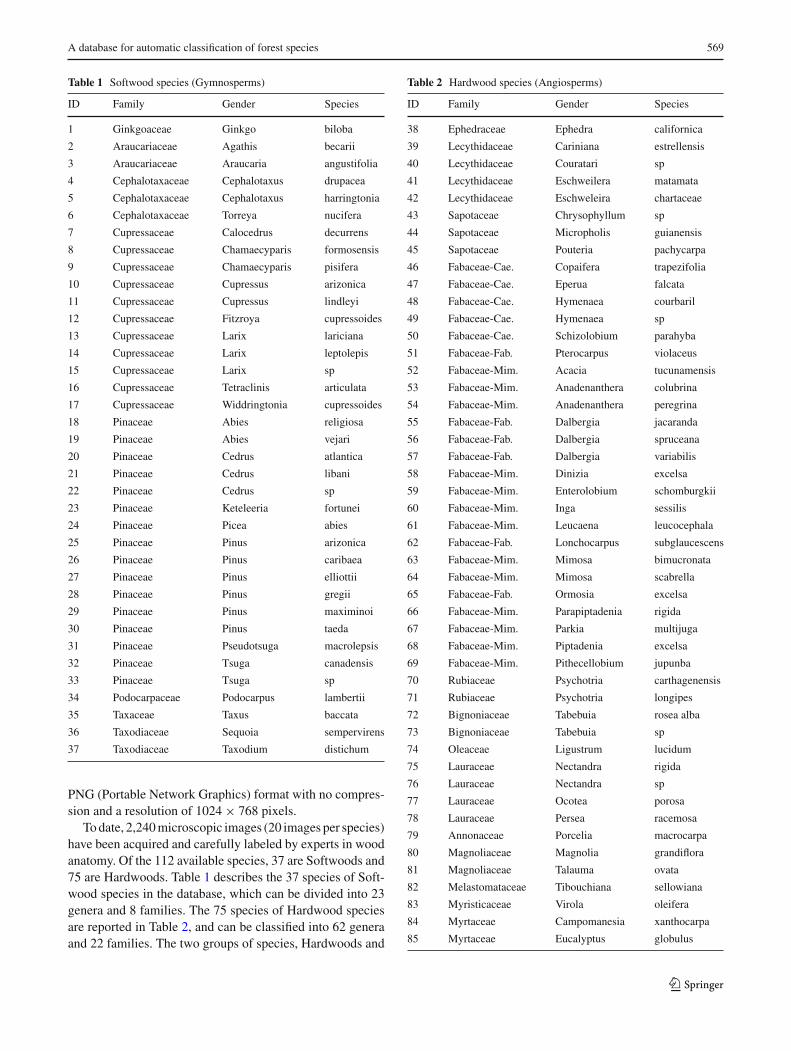
Figure 2 shows four different species in the database.It is worth noting that color cannot be used as an identi-fying feature in this database, since its hue depends on thecurrent used to produce contrast in the microscopic images.All the images were therefore converted to gray scale (256levels) in our experiments.

Looking at these samples, we can see that they have differ-ent structures. Hardwoods usually present some large holes,known as vessels (Fig. 2c, d), whereas Softwoods have a

more homogeneous texture (Fig. 2b) or present smaller holes,known as resiniferous channels (Fig. 2a).

Another visual characteristic of a of the Softwood speciesis the growth ring, which is defined as the difference in thethickness of the cell walls resulting from the annual devel-opment of the tree. We can see this feature in Fig. 2b. Thecoarse cells at the bottom and top of the image indicate moreintense physiological activity during spring and summer. Thesmaller cells in the middle of the image (highlighted in lightred) represent the minimum physiological activity that occursduring autumn and winter.

3 Features

In this section, we describe the three feature sets we usedto train the classifiers. The first was designed to explore thestructure of the wood. As mentioned above, if we take a closerlook at the images in the database, we can see that the twogroups differ in their structure. The other two feature sets weused, GLCM and LBP, are frequently applied to solve textureclassification problems. We describe these feature sets brieflybelow.

3.1 Structural features

One feature that is very often found in Hardwood species isthe vessel (Fig. 2c, d), which constitutes the major part of thewater transport system in the plant. Softwoods do not havesuch vessels, but resiniferous channels (Fig. 2a), which arevery similar to vessels, are quite common in these species.Therefore, this feature alone is not sufficient to discriminatebetween the two groups. Another aspect of the Hardwoodspecies is that they have a denser structure (smaller cells)than Softwoods. What we have observed in some experi-ments is that, after segmentation, the binary images of theHardwood species contain large connected components. Bycontrast, Softwoods have a large number of small connectedcomponents. Therefore, the rationale behind the creation ofthis feature set is to detect those connected components anddescribe their structure by using simple statistical measures.For this reason, we call it a structural feature set.

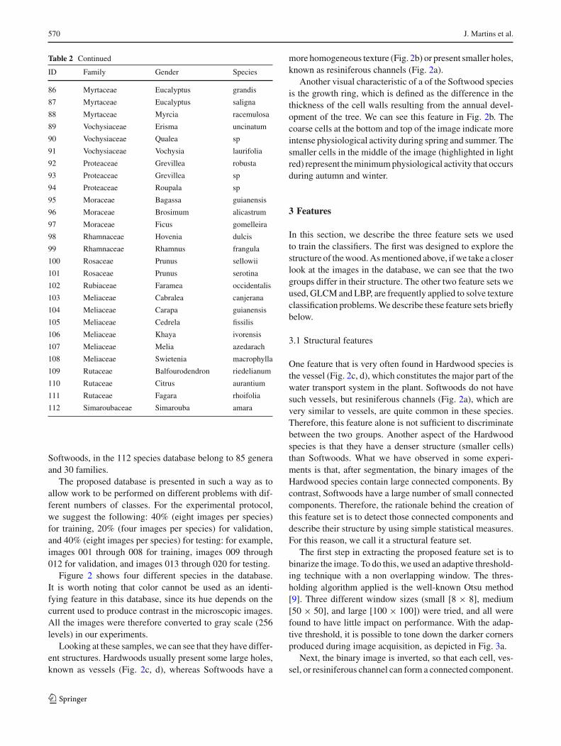
The first step in extracting the proposed feature set is tobinarize the image. To do this, we used an adaptive threshold-ing technique with a non overlapping window. The thres-holding algorithm applied is the well-known Otsu method[9]. Three different window sizes (small [8 × 8], medium[50 × 50], and large [100 × 100]) were tried, and all werefound to have little impact on performance. With the adap-tive threshold, it is possible to tone down the darker cornersproduced during image acquisition, as depicted in Fig. 3a.

Next, the binary image is inverted, so that each cell, ves-sel, or resiniferous channel can form a connected component.

123

A database for automatic classification of forest species 571

Fig. 2 Species of the database a 21, b 33, c 58, and d 95

Fig. 3 Feature extraction. a Gray-scale images, b binary images, andc connected components after erosion

In order to keep the main connected components and separatethose connected during the thresholding process, we appliedan erosion, which is a basic operator in the area of mathemati-cal morphology [10]. The structuring element employed was

the square (3 × 3) and the number of iterations was deter-mined empirically. In Sect. 4, we discuss the impact on therecognition rate of this operation and the number of iterationsrequired.

Figure 3 depicts this process. As we can see in Fig. 3c,a large number of components were removed by the erosionprocess. We can also see that the Hardwoods lost more com-ponents during this process than the Softwoods. The numberand size of the connected components allow us to discrimi-nate between the two classes.

The next step is to compute the features for the remainingconnected components. The feature vector is composed of thefollowing five elements: number of connected components,average size of the connected components, variance, kurto-sis, and obliquity. The features are then normalized using theMin–Max rule.

3.2 Gray level co-occurrence matrix (GLCM)

Among the statistical techniques available for texture rec-ognition, the GLCM has been one of the most widely usedand successful. This technique consists of statistical exper-iments conducted on how a certain level of gray occurs onother levels of gray [11]. It intuitively provides measuresof properties such as smoothness, coarseness, and regular-ity. Haralick [12], who originated this technique, suggesteda set of 14 characteristics, but most works in the literature

123

572 J. Martins et al.

Fig. 4 The original LBP operator

Fig. 5 The extended LBP operator [14]

consider a subset of these descriptors. In our case, we usedthe following six: Energy, Contrast, Entropy, Homogeneity,Maximum Likelihood, and 3rd Order Moment.

By definition, a GLCM is the probability of the joint occur-rence of gray-levels i and j within a defined spatial relationin an image. That spatial relation is defined in terms of a dis-tance d and an angle θ . From this GLCM, some statisticalinformation can be extracted. Assuming that Ng is the gray-level depth, and p(i, j) is the probability of the co-occurrenceof gray-level i and gray-level j observing consecutive pixelsat distance d and angle θ , we can use a GLCM to describewood texture.

In our experiments, we tried different values of d, as wellas different angles. The best setup we found is d = 5 andθ = [0, 45, 90, 135]. Considering the six descriptors men-tioned above, we arrive at a feature vector with 24 compo-nents.

3.3 Local Binary Patterns (LBP)

The original LBP proposed by Ojala et al. [13] labels thepixels of an image by thresholding a 3 × 3 neighborhoodof each pixel with the center value. Then, considering theresults as a binary number and the 256-bin histogram of theLBP labels computed over a region, they used this LBP as atexture descriptor. Figure 4 illustrates this process.

The limitation of the basic LBP operator is its small neigh-borhood, which cannot absorb the dominant features in large-scale structures. To overcome this problem, the operator wasextended to cope with larger neighborhoods. By using cir-cular neighborhoods and bilinearly interpolating the pixelvalues, any radius and any number of pixels in the neighbor-hood are allowed. Figure 5 depicts the extended LBP oper-ator, where (P, R) stands for a neighborhood of P equallyspaced sampling points on a circle of radius R, which formsa neighbor set that is symmetrical in a circular fashion.

The LPB operator LBPP,R produces 2P different binarypatterns that can be formed by the P pixels in the neighborset. However, certain bins contain more information than oth-ers, and so, it is possible to use only a subset of the 2P LBPs.Those fundamental patterns are known as uniform patterns.A LBP is called uniform if it contains at most two bitwisetransitions from 0 to 1 or vice versa when the binary stringis considered circular. For example, 00000000, 001110000and 11100001 are uniform patterns. It is observed that uni-form patterns account for nearly 90% of all patterns in the(8,1) neighborhood and for about 70% of all patterns ib the(16, 2) neighborhood in texture images [13,15].

Accumulating the patterns that have more than two tran-sitions into a single bin yields an LBP operator, denotedLBPu2

P,R , with fewer than 2P bins. For example, the num-ber of labels for a neighborhood of 8 pixels is 256 for thestandard LBP but 59 for LBPu2. Then, a histogram of thefrequency of the different labels produced by the LBP oper-ator can be built. We have tried out different configurationsof LBP operators, but the one that produced the best resultswas the LBPu2

8,2, with a feature vector of 59 components.

4 Experiments and discussion

An important aspect of pattern recognition problems that isvery often neglected is class distribution. A tacit assump-tion in the use of recognition rate as an evaluation metric isthat the class distribution among examples is constant andrelatively balanced. In the database we propose here, this isnot the case. In our context, receiver operating characteristic(ROC) curves are attractive because they are insensitive tochanges in class distribution. If the proportion of positive tonegative instances changes in a test set, the ROC curves willnot change [16]. For this reason, we present the ROC curvesand area under the curve (AUC) values for all the experi-ments. The AUC of a classifier has an important statisticalproperty: it is equivalent to the probability that the classifierwill rank a randomly chosen positive instance higher than arandomly chosen negative instance.

The overall error rate that has been used for evaluationpurposes in this work is given by Eq. 1.

Overall error rate = FP + FN

TP + TN + FP + FN(1)

where FP, FN, TP, and TN stand for false positive, false neg-ative, true positive, and true negative, respectively. Thesestatistics are defined in the 2 × 2 confusion matrix depictedin Fig. 6.

Hence, the recognition rate can be calculated using Eq. 2

Recognition rate = 100 − (Overall error rate × 100) (2)

123

A database for automatic classification of forest species 573

Fig. 6 2 × 2 confusion matrix

As pointed out earlier, three different classifiers were usedto assess these feature sets: k−NN, LDA, and SVM. For theSVM, different kernels were tried, but the Gaussian kernelproduced the best results. The kernel parameters γ and Cwere defined empirically through a grid search on the vali-dation set. In our experiments, the database was divided intotraining (40%), validation (20%), and testing (40%), as sug-gested before, i.e. the validation set is used in a holdout vali-dation scheme. In order to show that the choice of the imagesused in each subset does not have a significant impact on therecognition rate, each experiment was performed five timeswith different subsets (randomly selected) for training, vali-dation, and testing. The small standard deviation values showthat the choice of the images for each dataset is not an impor-tant issue.

The next two subsections report the experiments for the2-class problem and the multi-class problem, respectively.Then in Sect. 4.3 we show some results on different config-urations of the database.

4.1 2-Class problem

The first set of experiments was performed for the 2-classproblem using the structural feature set. Our first concernwas to determine the impact of the morphological operatoron feature extraction, and, consequently, on classifier per-formance. To do this, we extracted features using differentnumbers of iterations for the erosion operator. Figure 7 showsthe impact in terms of performance on the validation set forthe three classifiers. As we can see, all the classifiers behavein a similar way to the different numbers of iterations usedwith the erosion operator. For a small number of iterations,a large number of connected components is considered forfeature extraction. Aggressive erosion, by contrast, removesimportant components. This, of course, drastically reducesthe performance of all the classifiers. We found that the bestcompromise was achieved using six iterations.

The best results in this experiment were achieved by theSVM and k-NN with 93.1 and 92.6% of the recognition rateon the test set respectively. In the case of the k-NN, the bestvalue for k was 3. The LDA classifier had the worst per-formance, at 88.9% of the recognition rate. In all cases, we

Fig. 7 Impact of the erosion in the performance of the classifiers onthe validation set

Fig. 8 ROC curves for the classifiers trained with structural featureson the testing set

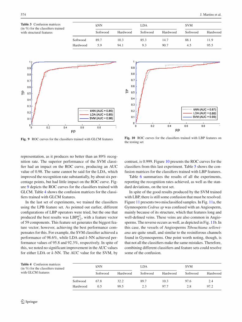
considered the features extracted from the images after sixiterations of the erosion operator. The results also show thatthe size of the window used for the adaptive thresholdinghas little impact on the final recognition rate. Figure 8 showsthe ROC curves and AUC values for all the classifiers. Inspite of the similar performance achieved by the SVM andk-NN classifiers in terms of recognition rate, we can see fromFig. 8 that the k-NN produces much higher false positive (FP)rates for any given true positive (TP) rate. Table 3 shows theconfusion matrices for the classifiers trained with structuralfeatures.

In the second series of experiments, all the classifierswere trained with the GLCM feature set. As in the previ-ous experiments, the SVM classifier outperformed the otherclassifiers, achieving a recognition rate of 97.4%. The LDAclassifier performed much better with this feature set, at95.0%, however the k-NN classifier seems unsuitable for this

123

574 J. Martins et al.

Table 3 Confusion matrices(in %) for the classifiers trainedwith structural features

kNN LDA SVM

Softwood Hardwood Softwood Hardwood Softwood Hardwood

Softwood 89.7 10.3 85.3 14.7 88.1 11.9

Hardwood 5.9 94.1 9.3 90.7 4.5 95.5

Fig. 9 ROC curves for the classifiers trained with GLCM features

representation, as it produces no better than an 89% recog-nition rate. The superior performance of the SVM classi-fier had an impact on the ROC curve, producing an AUCvalue of 0.98. The same cannot be said for the LDA, whichimproved the recognition rate substantially, by about six per-centage points, but had little impact on the ROC curve. Fig-ure 9 depicts the ROC curves for the classifiers trained withGLCM. Table 4 shows the confusion matrices for the classi-fiers trained with GLCM features.

In the last set of experiments, we trained the classifiersusing the LPB feature set. As pointed out earlier, differentconfigurations of LBP operators were tried, but the one thatproduced the best results was LBPu2

8,2, with a feature vectorof 59 components. This feature set generates the biggest fea-ture vector; however, achieving the best performance com-pensates for this. For example, the SVM classifier achieved aperformance of 98.6%, while LDA and k-NN achieved per-formance values of 95.8 and 92.3%, respectively. In spite ofthis, we noted no significant improvement in the AUC valuesfor either LDA or k-NN. The AUC value for the SVM, by

Fig. 10 ROC curves for the classifiers trained with LBP features onthe testing set

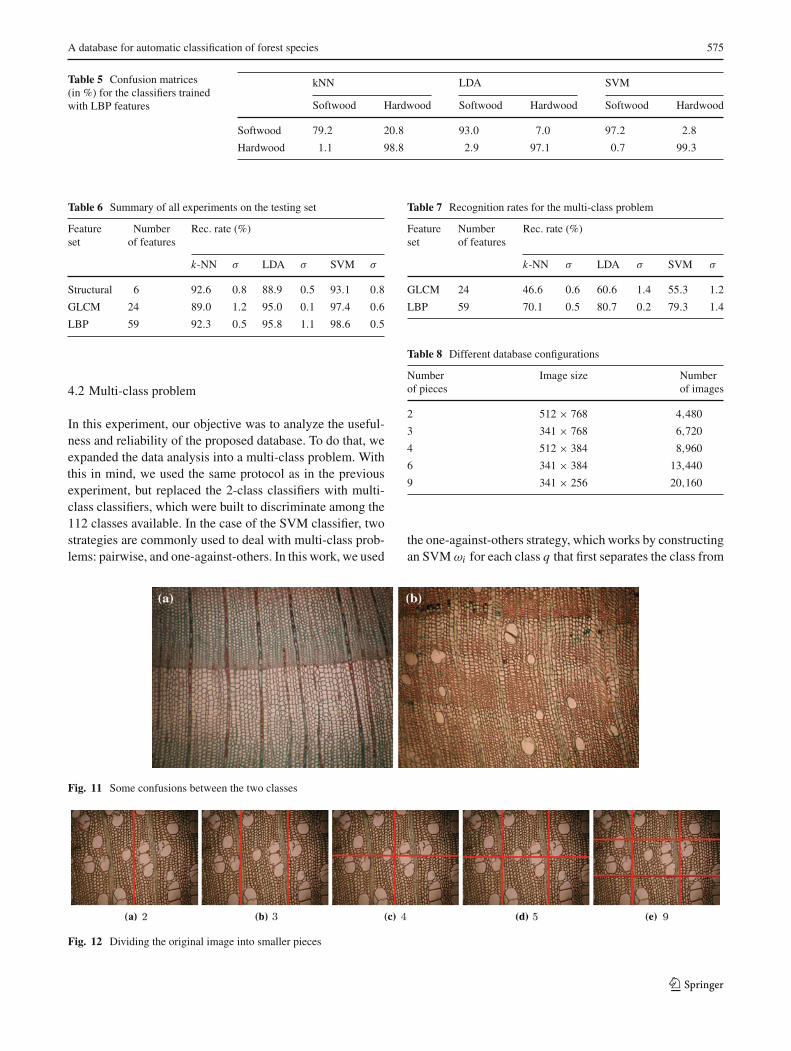
contrast, is 0.999. Figure 10 presents the ROC curves for theclassifiers from this last experiment. Table 5 shows the con-fusion matrices for the classifiers trained with LBP features.

Table 6 summarizes the results of all the experiments,reporting the recognition rates achieved, as well as the stan-dard deviations, on the test set.

In spite of the good results produced by the SVM trainedwith LBP, there is still some confusion that must be resolved.Figure 11 presents two misclassified samples. In Fig. 11a, theGymnosperm Cedrus sp was confused with an Angiosperm,mainly because of its structure, which that features long andwell-defined veins. These veins are also common in Angio-sperms. The reverse occurs as well, as depicted in Fig. 11b. Inthis case, the vessels of Angiosperms Tibouchiana sellowi-ana are quite small, and similar to the resiniferous channelsfound in Gymnosperms. One point worth noting, though, isthat not all the classifiers make the same mistakes. Therefore,combining different classifiers and feature sets could resolvesome of the confusion.

Table 4 Confusion matrices(in %) for the classifiers trainedwith GLCM features

kNN LDA SVM

Softwood Hardwood Softwood Hardwood Softwood Hardwood

Softwood 67.8 32.2 89.7 10.3 97.6 2.4

Hardwood 0.5 99.5 2.3 97.7 2.8 97.2

123

A database for automatic classification of forest species 575

Table 5 Confusion matrices(in %) for the classifiers trainedwith LBP features

kNN LDA SVM

Softwood Hardwood Softwood Hardwood Softwood Hardwood

Softwood 79.2 20.8 93.0 7.0 97.2 2.8

Hardwood 1.1 98.8 2.9 97.1 0.7 99.3

Table 6 Summary of all experiments on the testing set

Feature Number Rec. rate (%)set of features

k-NN σ LDA σ SVM σ

Structural 6 92.6 0.8 88.9 0.5 93.1 0.8

GLCM 24 89.0 1.2 95.0 0.1 97.4 0.6

LBP 59 92.3 0.5 95.8 1.1 98.6 0.5

4.2 Multi-class problem

In this experiment, our objective was to analyze the useful-ness and reliability of the proposed database. To do that, weexpanded the data analysis into a multi-class problem. Withthis in mind, we used the same protocol as in the previousexperiment, but replaced the 2-class classifiers with multi-class classifiers, which were built to discriminate among the112 classes available. In the case of the SVM classifier, twostrategies are commonly used to deal with multi-class prob-lems: pairwise, and one-against-others. In this work, we used

Table 7 Recognition rates for the multi-class problem

Feature Number Rec. rate (%)set of features

k-NN σ LDA σ SVM σ

GLCM 24 46.6 0.6 60.6 1.4 55.3 1.2

LBP 59 70.1 0.5 80.7 0.2 79.3 1.4

Table 8 Different database configurations

Number Image size Numberof pieces of images

2 512 × 768 4,480

3 341 × 768 6,720

4 512 × 384 8,960

6 341 × 384 13,440

9 341 × 256 20,160

the one-against-others strategy, which works by constructingan SVM ωi for each class q that first separates the class from

Fig. 11 Some confusions between the two classes

Fig. 12 Dividing the original image into smaller pieces

123

576 J. Martins et al.

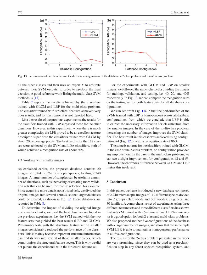
Fig. 13 Performance of the classifiers on the different configurations of the database. a 2-class problem and b multi-class problem

all the other classes and then uses an expert F to arbitratebetween their SVM outputs, in order to produce the finaldecision. A good reference work listing the multi-class SVMmethods is [17].

Table 7 reports the results achieved by the classifierstrained with GLCM and LBP for the multi-class problem.The classifier trained with structural features achieved verypoor results, and for this reason it is not reported here.

Like the results of the previous experiments, the results forthe classifiers trained with LBP surpassed those for the otherclassifiers. However, in this experiment, where there is muchgreater complexity, the LPB proved to be an excellent texturedescriptor, superior to the classifiers trained with GLCM byabout 20 percentage points. The best results for the 112 clas-ses were achieved by the SVM and LDA classifiers, both ofwhich achieved a recognition rate of about 80%.

4.3 Working with smaller images

As explained earlier, the proposed database contains 20images of 1,024 × 768 pixels per species, totaling 2,240images. A larger number of samples can be useful in a num-ber of situations, such as increasing or creating more valida-tion sets that can be used for feature selection, for example.Since acquiring more data is not a trivial task, we divided theoriginal images into several chunks, so that larger databasescould be created, as shown in Fig. 12. These databases arereported in Table 8.

To determine the impact of dividing the original imageinto smaller chunks, we used the best classifier we found inthe previous experiments, i.e. the SVM trained with the twofeature sets that yielded the best results (LBP and GLCM).Preliminary tests with the structural feature set on smallerimages considerably reduced the performance of the classi-fiers. This is mainly because important structural informationcan find its way into several of those smaller pieces, whichcompromises the structural feature vector. This is why we didnot pursue the experiments with the structural feature set.

For the experiments with GLCM and LBP on smallerimages, we followed the same scheme for dividing the imagesfor training, validation, and testing, i.e. 40, 20, and 40%respectively. In Fig. 13, we can compare the recognition rateson the testing set for both feature sets for all database con-figurations.

We can see from Fig. 13a, b that the performance of theSVMs trained with LBP is homogeneous across all databaseconfigurations, from which we conclude that LBP is ableto extract the necessary information for classification fromthe smaller images. In the case of the multi-class problem,increasing the number of images improves the SVM classi-fier. The best result in this case was achieved using configu-ration #4 (Fig. 12c), with a recognition rate of 86%.

The same is not true for the classifiers trained with GLCM.In the case of the 2-class problem, no configuration providedany improvement. In the case of the multi-class problem, wecan see a slight improvement for configurations #2 and #3.However, the enormous difference between GLCM and LBPmakes this irrelevant.

5 Conclusion

In this paper, we have introduced a new database composedof 2,240 microscopic images of 112 different species dividedinto 2 groups (Hardwoods and Softwoods), 85 genera, and30 families. A comprehensive set of experiments using threedifferent feature sets and three different classifiers has shownthat an SVM trained with a 59-dimensional LBP feature vec-tor is a good option for both 2-class and multi-class problems.We also proposed another five configurations of the databasewith a larger number of images, and show that the same tupleSVM-LBP, is able to maintain a homogeneous performancein all five configurations.

The results for the 2-class problem presented in this workare very promising, since they can be used as a preclassi-fication step in any forest species recognition system, and

123

A database for automatic classification of forest species 577

reduce the possible confusion between species of differentgenera and families. In future work, we plan to refine and testother feature sets to solve any remaining confusion, and usethis dataset to build a system to automatically identify forestspecies. Our expectation is that this database will contributeto the field of forest species recognition and motivate moreresearchers to work in this field.

Acknowledgments This work have been supported by The NationalCouncil for Scientific and Technological Development (CNPq)—Bra-zil grant #301653/2011-9 and the Coordination for the Improvement ofHigher Level Personnel (CAPES).

References

1. Thomas, L., Milli, L.: A robust gm-estimator for the auto-mated detection of external defects on barked hardwood logs andstems. IEEE Trans. Signal Proc. 55, 3568–3576 (2007)

2. Huber, H.A.: A computerized economic comparison of a conven-tional furniture rough mill with a new system of processing. For.Prod. J. 21(2), 34–39 (1971)

3. Buechler, D.N., Misra, D.K.: Subsurface detection of small voids inlow-loss solids. In: First ISA/IEEE Conference Sensor for Industry,pp. 281–284 (2001)

4. Tou, J.Y., Lau, P.Y., Tay Y.H.: Computer vision-based wood rec-ognition system. In : Proceedings of International Workshop onAdvanced Image Technology (2007)

5. Tou, J.Y., Tay, Y.H., Lau, P.Y.: One-dimensional grey-levelco-occurrence matrices for texture classification. In: InternationalSymposium on Information Technology (ITSim 2008), pp. 1–6(2008)

6. Tou, J.Y., Tay, Y.H., Lau, P.Y.: A comparative study for textureclassification techniques on wood species recognition problem. Int.Confer. Nat. Comput. 5, 8–12 (2009)

7. Khalid, M., Lee, E.L.Y., Yusof, R., Nadaraj, M.: Design of an intel-ligent wood species recognition system. IJSSST. 9(3) (2008)

8. Paula, P.L., Oliveira, L.S., Britto, A.S., Sabourin, R.: Forest spe-cies recognition using color-based features. In: International Con-ference on Pattern Recognition, pp. 4178–4181 (2010)

9. Otsu, N.: A threshold selection method from gray-level histo-gram. IEEE Trans. Syst. Man Cybern. 8, 62–66 (1978)

10. Serra, J.: Image Analysis and Mathematical Morphology. Aca-demic Press, New York (1984)

11. Tuceryan, M., Jain, A.K.: Texture analysis. The Handbook of Pat-tern Recognition and Computer Vision. World Scientific, Singapore(1998)

12. Haralick, R.M.: Statistical and structural approaches to texture.Proc. IEEE 67(5) (1979)

13. Ojala, T., Pietikainen, M., Harwood, D.: A comparative study oftexture measures with classification based on featured distribu-tion. Pattern Recogn. 29(1), 51–59 (1996)

14. Shan, C., Gong, S., McOwan, P.W.: Facial expression recognitionbased on local binary patterns: a comprehensive study. Image Vis.Comput. 27, 803–816 (2009)

15. Ojala, T., Pietikainen, M., Mäenpää, T.: Multiresolution gray-scale and rotation invariant texture classification with local binarypatterns. IEEE Trans. Pattern Anal. Mach. Intell. 24(7), 971–987 (2002)

16. Fawcett, T.: An introduction to ROC analysis. Pattern Recogn.Lett. 227(8), 861–874 (2006)

17. Hsu, C.-W., Lin, C.-J.: A comparison of methods for multi-classsupport vector machines. IEEE Trans. Neural Netw. 13, 415–425 (2002)

Author Biographies

J. Martins received his B.S.degree in Informatics from theWestern Paraná State University(UNIOESTE), 2000, Cascavel,PR, Brazil, and the M.E. degreein Production Engineering fromthe Federal University of SantaCatarina (UFSC), 2002,Florianópolis, SC, Brazil. In2003, he joined the Techno-logical Federal University ofParana (UTFPR) where he iscurrently an assistant professor.Since 2010, he is a Ph.D. can-didate at Federal University of

Parana (UFPR) investigating forest species recognition based on texturefeatures and microscopic images. His research interests include PatternRecognition and Image Analysis.

L. S. Oliveira received hisB.S. degree in Computer Sci-ence from UnicenP, Curitiba, PR,Brazil, the M.Sc. degree in elec-trical engineering and industrialinformatics from the Centro Fed-eral de Educação Tecnologica doParaná (CEFET-PR), Curitiba,PR, Brazil, and Ph.D. degree inComputer Science from Ecole deTechnologie Superieure, Univer-site du Quebec in 1995, 1998 and2003, respectively. From 2004to 2009 he was professor of theComputer Science Department at

Pontifical Catholic University of Parana, Curitiba, PR, Brazil. In 2009,he joined the Federal University of Parana, Curitiba, PR, Brazil, wherehe is professor of the Department of Informatics and head of the Grad-uate Program in Computer Science. His current interests include Pat-tern Recognition, Machine Learning, Image Analysis, and EvolutionaryComputation.

S. Nisgoski is Forest Engi-neer, received her M.Sc. andthe Ph.D. degrees in Forest Sci-ence, on Forest Products Uti-lization Technology from Fed-eral University of Parana, Brazil,in 1999 and 2005, respectively.Since 2009, she is an adjunct pro-fessor on Forest and EngineeringDepartment of same institution.Her research interests includewood and charcoal anatomy andidentification and material char-acterization by non destructivetechniques

123

578 J. Martins et al.

R. Sabourin received his B.Ing.,M.Sc.A., and Ph.D. degreesin Electrical Engineering fromthe Ecole Polytechnique deMontreal in 1977, 1980 and1991, respectively. In 1977, hejoined the physics department ofthe Universite de Montreal wherehe was responsible for the designand development of scientificinstrumentation for the Observa-toire du Mont Megantic. In 1983,he joined the staff of the Ecole deTechnologie Superieure, Univer-site du Quebec, Montreal, P.Q.

Canada, where he is currently a professeur titulaire in the Departementde Genie de la Production Automatisee. In 1995, he joined also the Com-puter Science Department of the Pontificia Universidade Catolica doParana (PUC-PR, Curitiba, Brazil) where he was corresponsible since1998 for the implementation of a Ph.D. program in Applied Informatics.Since 1996, he is a senior member of the Centre for Pattern Recogni-tion and Machine Intelligence (CENPARMI). His research interests arein the areas of handwriting recognition and signature verification forbanking and postal applications.

123