Detecting "Small" Mean Shifts in Time SeriesAuthor(s): John U. Farley and Melvin J. HinichSource: Management Science, Vol. 17, No. 3, Theory Series (Nov., 1970), pp. 189-199Published by: INFORMSStable URL: http://www.jstor.org/stable/2629088Accessed: 17/05/2010 16:09

Your use of the JSTOR archive indicates your acceptance of JSTOR's Terms and Conditions of Use, available athttp://www.jstor.org/page/info/about/policies/terms.jsp. JSTOR's Terms and Conditions of Use provides, in part, that unlessyou have obtained prior permission, you may not download an entire issue of a journal or multiple copies of articles, and youmay use content in the JSTOR archive only for your personal, non-commercial use.

Please contact the publisher regarding any further use of this work. Publisher contact information may be obtained athttp://www.jstor.org/action/showPublisher?publisherCode=informs.

Each copy of any part of a JSTOR transmission must contain the same copyright notice that appears on the screen or printedpage of such transmission.

JSTOR is a not-for-profit service that helps scholars, researchers, and students discover, use, and build upon a wide range ofcontent in a trusted digital archive. We use information technology and tools to increase productivity and facilitate new formsof scholarship. For more information about JSTOR, please contact support@jstor.org.

INFORMS is collaborating with JSTOR to digitize, preserve and extend access to Management Science.

http://www.jstor.org

MANAGEMENT SCIENCE Vol. 17, No. 3, November, 1970

Printed in U.S.A.

DETECTING "SMALL" MEAN SHIFTS IN TIME SERIES*

JOHN U. FARLEYt AND MELVIN J. HINICHt?

Analyzing time series data for evidence of changes in market conditions is a prob- lem central to development of a marketing information system. Examples are tracking field reports on competitors' prices and analyzing market share estimates computed from retail audits and consumer panel reports. These series may involve substantial random measurement error, and any changes, often small relative to this error, are difficult to detect promptly and accurately. One way to approach this problem is with techniques recently developed for handling time series with small stochastic mean shifts as well as random error. Two special procedures are compared in Monte Carlo analyses with a simpler data filtering and control-chart approach; the latter appears the most promising.

I. Introduction

Developing a marketing information system involves a variety of rather unique statistical problems; partial solutions are available for some of these problems, while no formal solutions are now available for others. For example, such problems face a group which is responsible for keeping management of a major petroleum company apprised of movements in competitors' prices for a wide array of products. Several types of data flow in at different intervals-daily, weekly, and monthly. Some data are reported from within the firm, others come from commercial data collection sources and still others from numerous government agencies. The data inputs are subject to various reporting errors and distortions which might be considered random error or "noise". Prices in these markets may shift discretely rather than drifting up and down, and there may be a substantial time lag between a de facto change in price by one com- petitor and a public announcement that such a change has taken place. Tracking these price series for evidence of changes in competitive conditions is thus a major function of the information system.

The process is complicated by the fact that there may be several thousand separate series to track, and only a handful of the array can possibly receive explicit attention at any one time. To function smoothly and promptly, the computer-based information system requires built-in statistical procedures which seek evidence of shifts in these many series. Prompt, accurate evaluation of current conditions is vital. It is important to identify bona fide changes as soon as possible to initiate tactical response to changed conditions, but it is likewise important to avoid needlessly initiating major shifts in price or advertising which might be unprofitable or which might lead to degeneration of a stable market equilibrium. The need for speed dictates response as soon as possible, while the need for accuracy suggests waiting for as many observations as possible to be sure that a change has actually occurred. Besides tracking prices, similar problems occur in connection with detecting significant shifts in company sales series or in changes in market shares reported by panels or audits [5]. Such shifts are also often infrequent, discrete and subtle. It is tempting to develop and implement ad hoc statistical proce- dures in an attempt to balance off these two types of risks, but there are a variety of

* Received June 1969; revised December 1969, February 1970. t Columbia University. t Carnegie-Mellon University. ? The authors are grateful for the valuable criticisms of Professor T. W. McGuire.

189

190 JOHN U. FARLEY AND MELVIN J. HINICH

such procedures to choose among and there are also a number of statistical techniques with known properties which might be especially well suited for these purposes.

The most direct statistical analogy to the problem just described is to consider that each series is subject at any point of time to random parameter change which is small relative to the variance of measurement errors. It is important to distinguish this prob- lem from other parameter shift problems which should be handled quite differently. For example, if a parameter shift is very large relative to the variance of the measure- ment error, simple visual examination of the series will in all likelihood find a shift immediately. Similarly, if the position of any potential shift is pinpointed and only its existence at that point uncertain, regression techniques provide tests of whether a shift in fact occurred with very good properties [2].

However, the problem is quite different if a shift is likely to be small relative to the measurement error variance and if the analyst, unsure whether a shift occurs at all, thinks that one might occur at any point in the series.

II. The Mean-Shift Problem

Formally, the tracking problem is modeled as a stochastic shift in the mean of a time series. A stochastic process, X (t) =0 (t) + N (t), generates sequence data, where where 0(t) is a mean parameter (possibly shifting, possibly stable) and N (t) is sta- tionary Gaussian noise with zero mean and a known covariance function, 2. Any discrete parameter change can be modeled as a step function. For i = 1, 2, **,

(1) 0(t) = 0 when t*-1 < t ? t/*.

It is useful to assume that the number of points when 0 changes (the ti*) per unit time are Poisson 'distributed with a shift rate parameter, y, which is assumed known [6]. (The change rate, as we shall see, is very important and will cause considerable dif- ficulty in dealing with this problem. In particular, -y is seldom known in applications like those discussed in ?I.) 0(t) is thus the expected value of X (t), and it changes from one constant value to another at random times tO.

This paper uses artificial data to examine the behavior of three -alternative estima- tion procedures-two especially developed to deal with this particular problem and one based on more general filter techniques. The paper also examines two processing procedures-one in which a finite number of discrete observations of the series are formed into a finite record which is processed as a whole, and the other in which the series is considered as a running record and processed with filter techniques. The filter technique is based on procedures resembling control charts on filtered data produced by smoothing raw data.

III. The Discrete Observation, Fixed Record Case

The time series is viewed as if it were drawn during nonoverlapping periods nS time units long. Each record consists of n successive observations of X (t) where the ob- servations are taken S time units apart. If nS, the record length, is smaller than 'y-1, the mean time between shifts, the possibility of two or more shifts in a record can be disregarded. The sample points constitute the random vector {X1, ... , X1,, where each Xi is the value of the random process X (t) = 0 (t) + N (t) at time ti. The mean is a step function,

0 (t) = 0 if t < t*,

(2) =0+I ift>t

DETECTING "CSMALL"Y MEAN SHIFTS IN TIME SERIES 191

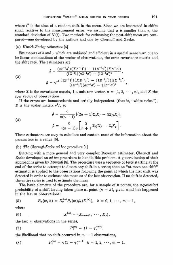
where t* is the time of a random shift in the mean. Since we are interested in shifts small relative to the measurement error, we assume that ,u is smaller than a, the standard deviation of N (t). Two methods for estimating the post-shift mean are com- pared-one developed by the authors and one by Chernoff and Zacks.

(a) Hinich-Farley estimators [6].

Estimators of 0 and A which are unbiased and efficient in a special sense turn out to be linear combinations of the vector of observations, the error covariance matrix and the shift rate. The estimators are

= (a2'a') (X2'1') - (12 a) (X2'a')

03 (12-1) (a'-la') -(-la )2

(3) -1A ( 121') (X2-la')- (12-a') (X'-11') A =vl (11-11/)(al-lat)- (12-1af)2

where 2 is the covariance matrix, 1 a unit row vector, a = {1, 2, * , n}, and X the row vector of observations.

If the errors are homoscedastic and serially independent (that is, "white noise"), 2 is the scalar matrix ur21, so

A 2 0 =n(n - [(2n + 1)YjXj -3YjjXj],

(4) n(n [ 1j

n(n -1 , n + 1 jX-X].

These estimators are easy to calculate and contain most of the information about the parameters in a range [6].

(b) The Chernoff-Zacks ad hoc procedure [1]

Starting with a more general and very complex Bayesian estimator, Chernoff and Zacks developed an ad hoc procedure to handle this problem. A generalization of their approach is given by Mustafi [8]. The procedure uses a sequence of tests starting at the end of the series to attempt to detect any shift in a series; then an "at most one shift" estimator is applied to the observations following the point at which the first shift was detected in order to estimate the mean as of the last observation. If no shift is detected, the entire series is used to estimate the mean.

The basic elements of the procedure are, for a sample of n points, the a-posteriori probability of a shift having taken place at point (n - k), given what has happened in the last m observations:

(5) Bn(m, k) = Dn-'lPk(m)VkI(X(m)), k = 0, 1, ., m- 1,

where

(6) X(mn = {Xn_m+l X ... * Xn}X

the last m observations in the series,

(7) ) = (1 -

the likelihood that no shift occurred in m - 1 observations,

(8 ) P(m) = _ (1 _ )m2 k =1, 2, ... , m-1,

192 JOHN U. FARLEY AND MELVIN J. HINICH

the likelihood that one shift did occur. (This assumes, as did the Hinich-Farley es- timators, an equal likelihood of a shift between any two points.) Further,

(9) [m + a2k(m-k)]i 2 mk( k (m)-

for k = O, 1, n - 1,

in which a is the size of the shift and y is the shift rate parameter as before. Expression (9) also involves two partial means,

(10) x(m) = =n--

and

(11) im- = 1 *+l Xi

further weighted to form

(12) Dm* = l k=oPkm)k (Xm)

Using Km as the value of k which maximizes Bn (m, k), the ad hoc procedure consists of computing K2, K3, X until Km # 0 is reached, say at K*. This means it is more likely that a shift occurred at K* than that no change occurred at all from K* on. Then an "at most one change" Bayes estimator is applied to the observations Xn-K*+l,

Xn_K *+2 X * *X Xn to estimate the mean. This Bayes estimator for large a, n** is closely related to the detector (Kn):

** (D**)-l rPo __n_ 1 n_m ln= (D

)UXn-m (13) t~~~ni N/ m~(n - m)

( exp [1 m(n- m) (if -X*_)2

where D** is the limit of D* as a- -* oo, i.e.,

(14) D** =P + Z Em Pm exp F!m(n m)(Xm-im)21

The Chernoff-Zacks procedure is more complex than the Hinich-Farley procedure, but there is a distinct appeal to attempting to detect the shift and to disregarding data be- fore it in estimating the mean.

IV. Monte Carlo Analysis of the Procedures

Several false starts with actual marketing data showed that there was too much specification uncertainty to provide an adequate test of the procedures' performance, and artificial data of known configuration provided a more natural starting point. The performance of the two estimators was compared using series of 100 observations with errors (N (0, I)), generated by the method discussed by Kronmal [7]. GO = 0 for all series-that is, the initial mean was zero. Five values of the y were used, and the size of the shift was .5 (half the standard deviation of the noise). Single shifts occurred in half of the series; half of the shifts were positive and half were negative, with the signs randomized. The shift positions were randomized rectangularly, producing an equal probability of a shift occurring at any point.

DETECTING "SMALL") MEAN SHIFTS IN TIME SERIES 193

Table I contains measures summarizing how the two techniques performed under various circumstances. The Hinich-Farley estimators are relatively straightforward to evaluate. The means of 0 are centered about the true value (zero), but the standard deviations are large, given the relative luxury of 100 data points. The jump heights, on the other hand, are not estimated well in general. The signs are right, but the estimated values are sensitive to 'y (which shows up in the denominator of (4)), and the result is a tendency for the , to become larger as the likelihood of a change decreases. The stand- ard errors of ,i also are related to 'y. The basic problem involves sensitivity to the specification of the change rate. For small y, the estimator is overly sensitive to shifts. For large -y, there is high likelihood of more than one jump leading to an underestimate of the shift size. When the expected number of shifts in the series corresponds to the actual number (i.e., -y = .01) the procedure works quite well, but is it not robust with respect to errors in specification of -y.

While the Hinich-Farley technique attempts to estimate jointly the level of the mean at the beginning of the series as well as the size of the change (if any), the Chernoff- Zacks technique starts at the end of a series, searches back for a change in mean, and then estimates the mean value of the series forward from the point at which such a change is found. In this case, the performance of both the detector and of the mean level estimator are important. Table 1 indicates that the detector is also sensitive to the probability of change. This is a case of the common statistical problems of two types of error where discrimination power is weak. When the probability of change is high the detector finds changes with approximately equal likelihood whether or not there is a change. When the probability of a change is small, fewer changes are detected in cases where none occurred, but the detector errs by failing to find changes when they do occur. Regardless of the change rate, though, there is large average error in the posi- tion where a change is detected and the variance of this error is also large.

Despite the weak performance of the detector, the estimator works reasonablv well whether or not the detector is used.

1. Using the detector. The estimates when no shift occurred are somewhat inferior to the Hinich-Farley statistics, both in terms of bias and squared error. When the mean shifts, the Chernoff-Zacks technique is superior in terms of bias, although standard errors are similar. It should be noted, however, that much more computer time is required by the Chernoff-Zacks technique-especially when -y is small and the detector searches back over a large part of most series in search of a shift.

2. Without the detector. Surprisingly, the estimator performed as well or better in terms of variance as it did when the detector was used. Of course, a bias towards zero is introduced in the cases where change occurs by the fact that a considerable amount of pre-shift data is retained on average.

That the Hinich-Farley and Chernoff-Zacks techniques perform similarly is hardly surprising, because the structure in both cases involves manipulations of Ji iXi and the change rate (ey) as the basic components of the analysis. This structure is intuitively appealing because, given equal likelihood of a shift in any interval, later observations in a series contain more information as it becomes increasingly likely that a shift has occurred somewhere before that observation.

Despite desirable theoretical properties, though, the performance is rather dis- appointing, largely due to sensitivity to the change rate (-y), which is usually unknown and very difficult to estimate. When the expected time between shifts is equal to the record length (that is, y = .01) the Hinich-Farley procedure out-performed the Chernoff-Zacks procedure in terms of bias and estimation error variance. Further,

194 JOIIN U. FARLEY AND MELVIN J. HINICHI

o - I U,,: ,, m 1- 'm 00 to 00 X

I~~~~~~~~~~~~~~~~~~ ..I = ":

. oFoO o m eq m

to 00

I0 I I e 1- 1-4

O q 00 U,,: o t C; Z ^1e t- 0 cq "

>~~~~~~~~~~~~~~~U: t- -- m t o C: -4 I to t- to _

Ei t - I: t- ? t co to I .t o I o o o ts > t X < ? O t e o >o

> I e:> e~~~~~~~~~o o _Z

| |- t O > n ? D >~~~~~~0 e t gt

00 t Oc ; - ko<?

-I t - co C". f

D oo Ci O ?? ? ? e> S v - v D eCD| 4

I~~~~~~~~~~~~l O O z< Cl! _#

r k E = S:: i U F a t0, O ? O o S u a" CD -

DETECTING "SMALL Y MEAN SHIFTS IN TIME SERIES 195

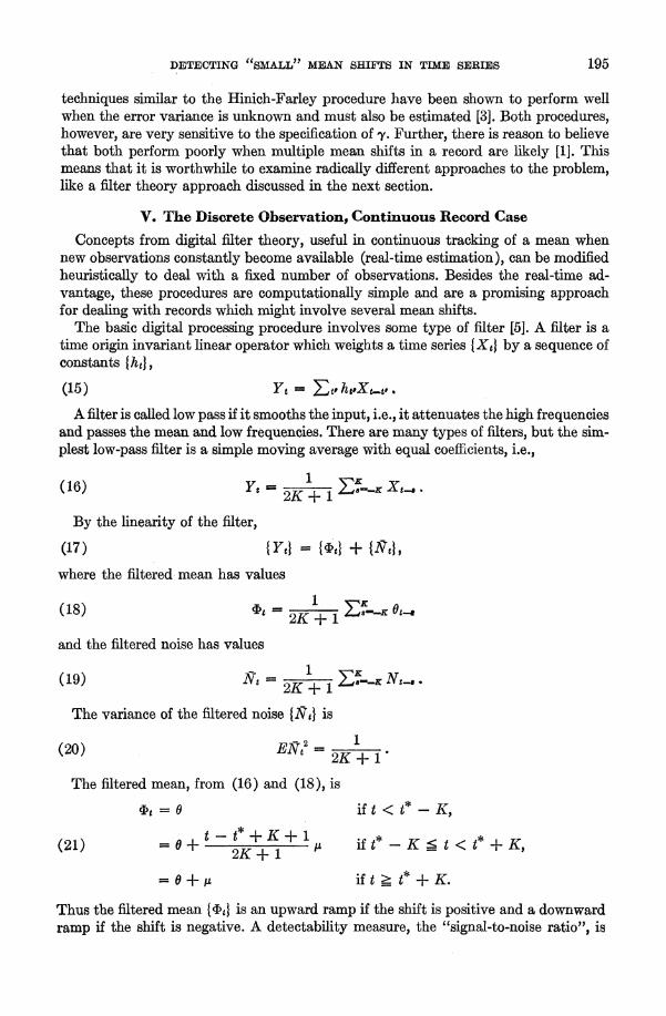
techniques similar to the Hinich-Farley procedure have been shown to perform well when the error variance is unknown and must also be estimated [3]. Both procedures, however, are very sensitive to the specification of y. Further, there is reason to believe that both perform poorly when multiple mean shifts in a record are likely [1]. This means that it is worthwhile to examine radically different approaches to the problem, like a filter theory approach discussed in the next section.

V. The Discrete Observation, Continuous Record Case

Concepts from digital filter theory, useful in continuous tracking of a mean when new observations constantly become available (real-time estimation), can be modified heuristically to deal with a fixed number of observations. Besides the real-time ad- vantage, these procedures are computationally simple and are a promising approach for dealing with records which might involve several mean shifts.

The basic digital processing procedure involves some type of filter [5]. A filter is a time origin invariant linear operator which weights a time series {Xt} by a sequence of constants {ht},

(15) Yt ,t=ht,Xt.t

A filter is called low pass if it smooths the input, i.e., it attenuates the high frequencies and passes the mean and low frequencies. There are many types of filters, but the sim- plest low-pass filter is a simple moving average with equal coefficients, i.e.,

(16) Yt = 2K+1 Xt_8

By the linearity of the filter,

(17) {Ye} = {1b} + {Sd, where the filtered mean has values

= 1 E18K - (18) (t 2K + 1 9-z Oz_

and the filtered noise has values

(19) St= 2K +1l-X Nt_

The variance of the filtered noise {SR} is

(20) Egt = 2K + 1

The filtered mean, from (16) and (18), is

if t < t*-K,

(21) =0+ 2K+ 1 if t*-K 9 t < t* + K,

= 8 + ,u if t > t* + K.

Thus the filtered mean {4t is an upward ramp if the shift is positive and a downward ramp if the shift is negative. A detectability measure, the "signal-to-noise ratio", is

196 JOHN U. FARLEY AND MELVIN J. HINICH

the size of shift divided by the standard deviation of the noise. If Dr denotes the de- tectability of the mean in {Xt} and Do the detectability of the mean in { Yd},

(22 ) Dr =

and

(23) Do = ,(2K + 1)1

from (20). The "gain" in filtering is defined as the ratio of detectabilities Do/Dr. In this case, the gain is

Do/Dr = (2K + 1)1.

By choosing K sufficiently large, the variance of {N } can be made much less than the amount of shift g, and a shift can be detected with probability approaching one. The trade-off is quite apparent; if K is made larger in order to reduce the variance of the estimated mean to improve the gain, detection is delayed.

The simple low pass filter in (16) is one of a variety of 2K + 1 coefficient filters which attenuate the high frequencies; some produce an even greater filter gain for the shift detection. For example, gain is increased by filtering the process twice with the filter in (16), which reduces the noise variance from (2K + 1)'1. Thus, the gain is Do/Dr = (1.5)2 (2K + 1)1, about 23 per cent more than in the simple filter. However, it also requires more data to produce a filtered record of length n than does the simple rectangular filter. The choice of filters available is endless, although most common are rectangular, triangular and exponential. The rectangular filter is chosen here for purposes of convenience.

VI. Monte Carlo Analysis of the Rectangular Filter

Heuristic decision rules were used for detection by starting at the end of the series and searching backward for a shift point. Such rules, useful in developing and testing control-chart procedures [7], avoid the problems in specification of the shift rate ('y) mentioned earlier. If a shift is detected at to, observations of Xt preceding to (for t < to) are discarded in estimating the current mean, since they should not yield any information about its new value. Artificial data also were used to test the filtering pro- cedure. Eight sets of 100 series { Yt}, each containing 90 observations smoothed rec- tangularly with K = 5, were constructed using methods similar to those described in ?IV. The decision rules all involve identifying a shift at to if p out of q observations Yto, Yo+l, * ... Yto+0-l are greater than T or less than - T (p and q are integers such that 1? p ? q). Four rules were used for each of 2 levels of T (T = .5 and T = .65); p = 3, q = 4; p = 4, q = 5; p = 5, q = 6; and p = 6, q = 7. If a shift is detected at to, the new mean is then estimated by a simple average of the input observations {Xt} taken from to to the end of the series. If the decision rule does not detect a shift as it goes backwards over the series, the estimate of the mean is given by an average of all values of the input series. This detection-estimation procedure is similar in spirit to control chart procedures common in quality control [8], and will be robust with respect to the shift rate y provided it is not too high and if the variance cr2 is stable.

Summary measures describing this analysis are shown in Table 2. With the looser decision rules (smaller p and q, and lower threshold value) the filter "detects" shifts in a high proportion of the series, regardless of whether one occurred. As p and q become larger and as the threshold is raised, fewer shifts are found in any series. Vary- ing p, q, and T in any application will thus allow explicit trade-off between both

DETECTING cSMALL J) MEAN SHIFTS IN TIME SERIES 197

TABLE 2 Summary Measures for Filter-Estimation Procedure

Absolute difference DECISION RULE Cbetween actual Estimated value of Number

DECISION RIJL:Ef Change Posthon where change position series after filter of obser- foun chonge as fund and where filter found a change vations detected change

3 of 4 > T or < -T T= .5 A =0 34 40.7 NA .0354 49

(28.483) (.1674) A = +.5 30 NA 20.8 .3613 31

(22.0819) (.2539) a = - .5 19 NA 19.526 -.39021 20

(26.435) (.1939) T= .65 A =0 17 51.82 NA -.0147 51

(28.76) (.0736) A = +.5 23 NA 15.52 .4810 27

(21.69) (.2830) A - - .5 18 NA 9.83 -.4735 22

(11.92) (.2393) 4 of 5 > T or < -T

T= .5 A =0 34 44.76 NA .0392 49 (29.09) (.1544)

A = +.5 27 NA 17.11 .4547 29 (18.55) (.1661)

a = - .5 20 NA 16.6 -.4022 22 (24.60) (.1798)

T= .65 A= 0 9 52.78 NA -.00342 51 (23.11) (.1066)

a = +F .5 23 NA 15.000 .4945 27 (14.67) (.2995)

A= -.5 17 NA 18.42 -.3945 22 (15.81) (.1829)

5 of 6 > T or < -T T = .5 A 0 26 44.88 NA .0384 51

(26.03) (.2459) A = +.5 26 NA 20.38 .4101 27

(22.81) (.1945) a = - .5 20 NA 18.80 -.4030 22

(20.98) (.2131) T= .65 A =0 5 61.4 NA .00676 51

(25.67) (.1174) a - +t .5 22 NA 15.54 .4802 27

(16.33) (.2375) 16 NA 13.06 -.3944 22

(20.47) (.1929) 6 of 7 > T or < -T

T= .5 A 0 21 49.76 NA .0325 51 (25.44) (.08011)

A _ +- .5 25 NA 16.24 .4803 27 (17.98) (.2403)

A = -.5 17 NA 18.00 -.4204 22 (25.09) (.2142)

T= .65 = 0 3 47.66 NA .0156 51 (23.03) (.1195)

A = ?.5 15 NA 22.6 .4496 27 (16.57) (.2505)

15 NA 18.87 -.4601 22 (12.96) (.2327)

198 JOHN U. FARLEY AND MELVIN J. HINICH

types of errors as well as the time required for detecting a change. In contrast to the results in ?IV, though, there is increasing discriminatory power (especially for the higher threshold), indicating that the filter techniques are preferable to those described in the last section. Errors in locating the position of shifts are comparable over thresh- olds and decision rules, indicating again that precise estimation of the point of shift is, not possible when the error variance is large and the time uncertainty of the shift is great. The estimated mean values using the filter are less biased than those presented in ?IV and their standard errors are smaller. As with the earlier results, however, there is an estimation bias towards zero when a shift does occur caused by asymmetric error in the filter, which tends to pass by a change a considerable distance before finding it.

VII. Discussion

Some ways have been examined to systematically track time series which potentially contain small stochastic mean shifts as well as random measurement errors. A "small shift" is one which is small relative to measurement error. Such problems may arise in an information system which monitors large numbers of data series, such as competitors' prices and advertising behavior, reported by representatives in the field or by other data collecting sources such as store audits or consumer panels. Three approaches were tested with artificial data using mean shifts which were rather small-that is, mean shifts which were half the magnitude of random measurement error variance. Two techniques (one developed by the authors and the other by Chernoff and Zacks) in- volved formal estimation under the assumption that there was at most one discrete jump in a data record of fixed length of the type often stored in an information system. Both techniques performed reasonably when the rate of shift occurrence was known, but both techniques are very sensitive to prior specification of the rate at which shifts oc- cur in terms of both classes of errors-that is, missing shifts which occur and identify- ing "shifts" which do not occur. Knowing the shift rate precisely and knowing that more than one shift in a record is extremely unlikely are two very severe restrictions for many applications.

A simpler filter technique was tested similarly with more promising results in terms of avoiding both classes of errors. The filter approach involved first smoothing the series and then implementing ad hoc decision rules based on consecutive occurrences of smoothed values falling outside a predetermined range about the running mean. These ad hoc procedures are unsatisfactory from the point of view of certain theoretical con- siderations, although it is important to note that the Chernoff-Zacks procedure had ad hoc elements, despite its over-aUl complexity and sophistication. This data filtering route appears to be the most promising way now available to approach the development of tracking procedures for information systems when the change rate is unknown. The superiority is due to flexibility, insensitivity to rates at which shifts occur over time, ability to be developed towards the possibility of multiple shifts in a record and clear statement of trade-offs of various types of errors.

References

1. CHERNOFF, H. AND ZACKS, S., "Estimating the Current Mean of a Normal Distribution which is Subjected to Changes in Time," Ann. Math. Statist., Vol. 35 (1964), pp. 999-1018.

2. CHOW, G., "Tests of Equality Between Two Sets of Coefficients in Two Linear Regressions," Econometrica, Vol. 28 (1960), pp. 591-605.

3. FARLEY, J. AND HINICH, M., "A Test for a Shifting Slope Coefficient in a Linear Model," to appear in The Journal of the American Statistical Association, forthcoming.

4. - AND -, "Tracking Marketing Parameters in Random Noise," Marketing and Economic Development, P. D. Bennet, ed., American Marketing Association, 1965, pp. 365-369.

DETECTING "SMALL ' MEAN SHIFTS IN TLME SERIES 199

5. GRENANDER, U. AND ROSENBLATT, M., Statistical Analysis of Stationary Time Series, John Wiley, New York, 1957.

6. HINICH, M. AND FARLEY, J. "Theory and Application of an Estimation Model for Time Series with Nonstationary Means," Management Science, Vol. 12 (1966), pp. 648-658.

7. KRONMAL, R., "The Evaluation of a Pseudo-Random Normal Generation," Journal of the As- sociation for Computing Machines, Vol. 11 (1964), pp. 357-363.

8. MUSTAFI, C. K., "Inference Problems about Parameters which are Subjected to Changes over Time," Ann. Math. Statist., Vol. 39 (1968), pp. 840-854.

9. ROBERTS, S. W., "A Comparison of Some Control Chart Procedures," Technometrics, Vol. 8 (1966), pp. 411-430.