Embed Size (px)
Citation preview

1
Distinguishing the Role of Authority “In” and Authority “To”
Dan Silverman
Joel Slemrod
Neslihan Uler
University of Michigan
May 9, 2012
Abstract: Authority, and the behavioral response to authority, is central to many important questions in public economics, but has received insufficient attention from economists. In particular, research has not differentiated between legitimate coercive power and the presumption of expert knowledge, what we call “authority to” and “authority in.” In this paper we report on the results of a series of lab experiments designed to distinguish the effects of the two sources of authority on contributions to a public project. The results suggest that authority “to” and authority “in” interact in ways not heretofore understood. Coercion without expert explanation does not increase voluntary contributions, nor does explanation without coercion, but together they induce more contributions than any other combination of policies. We interpret these findings to indicate that the reaction to an authority depends on whether that authority is perceived to be legitimate.
We thank Dennis Davis, Jiang Jiang, and Subhashini Venkatramani for able research assistance. For helpful comments on an earlier draft we thank Jim Alm, Rupert Sausgruber, and Christian Traxler as well as participants at presentations at the University of Michigan Public Finance Free Lunch Seminar, the Office of Tax Analysis at the U.S. Treasury Department, and the Workshop in Experimental Labor Economics at the University of Vienna.

2
1. Introduction and Motivation A wide range of behaviors raises doubts about whether, in all situations, individuals
successfully pursue their self-interest. Many people are attracted to default options, say on
pension offerings from their employer.1 People often forgo financial education, even when it is
inexpensive to obtain and when having it would substantially change their behavior.2 Some
dutifully comply with the tax system, even though the odds of being detected and penalized
suggest that some evasion would be optimal.3
The idea that people respond to authority provides a unifying explanation of these, and
many other, behaviors. Employees choose the default pension plan because they infer that their
employer, a benign authority figure with financial expertise, has chosen in their interest.
Workers save more after receiving employer-sponsored financial education because an
authoritative instructor emphasized the importance of planning for retirement. Households
comply with their tax liability in the face of a favorable tax evasion “lottery” because the tax
“authority” has instructed them to do so and may sanction them if they do not; plus households
know that by collecting taxes to provide services, the government may benefit them.
We believe that authority, and the behavioral response to authority, is central to many
important questions in public economics, but has received insufficient attention from economists.
Its relative absence is surprising given the recent wave of interest by economists in psychology,
and the historical prominence—indeed notoriety—of the experiments on authority and obedience
by Stanley Milgram (1974). Milgram famously showed that, when prompted by a white-coated
authority figure, subjects were often quite willing to administer what were apparently painful
shocks to people (who were actually confederates of the experimenter) behind a glass door.
Subsequent commentators, notably Morelli (1983), differentiated between legitimate coercive
power and the presumption of expert knowledge; we refer to these aspects of authority as
“authority to” and “authority in,” respectively. Reaction to the former may be characterized as
“obedience,” while response to the latter might be better denoted as “deference.” Neither kind of
response need be a “mistake;” responding to authority does not require that people care about
anything but consumption of standard goods and services.
1 See, for example, Madrian and Shea (2001), Choi, Laibson, Madrian, and Metrick (2004), and Beshears, Choi, 2 Lusardi and Mitchell (2007), Bernheim and Garret (2003), and Martin (2007) investigate the consequences of financial knowledge and education. 3 Feld and Frey (2002) discuss this issue.

3
While responding to the incentives or information offered by an authority may be rational,
we suspect that people will respond differently to the same actions, depending on whether those
actions were taken by a (government) authority or by an individual. Many experimental results,
such as those reported in Blount (1995), suggest that beliefs about what motivated another
person and about the appropriateness of those motives, their “intentionality,” are critical to
explaining behavior toward that person. Furthermore, ultimatum games with multiple players
suggest that responders care about whether proposers are unfair to them, but do not care much
about how the proposer treats others. We note that government policies often do not single out
particular individuals other than through enforcement actions. Thus, a key unanswered question
is the extent to which individuals ascribe human qualities like kindness, meanness, or distrust to
a (government) authority and react in similar ways as they do to other individuals who exhibit
these characteristics.
In this paper we report on the results of a series of lab experiments designed to
distinguish the effects of the two sources of authority described above on contributions to a
public project. We adopt a lab-based, experimental approach because we want, eventually, to
develop and refine hypotheses about the role of authority in economic decision-making.
Distinguishing these aspects of authority is inherently difficult to do with observational study; it
is hard to find circumstances where these features of government or authority have been
randomized across jurisdictions. In the lab, however, one must of course be careful to
distinguish the effects of the experimenter’s scrutiny and authority from the effects of other
sources of authority.
We focus on a public-goods experiment in particular because we hypothesize that the
details of the economic environment are likely to affect the influence of authority on individual
behavior. If so, gathering observations from specific environments will be useful and a public
goods problem is an attractive place to start. One attraction of this setting is that lab-based
public goods experiments have been studied extensively, so our findings can be compared with a
variety of benchmarks. In addition, the setting of public goods experiments resembles a broad
set of important public economics applications, including tax compliance and charitable
contributions.

4
Our experiments are designed to distinguish the effects of two sources of a government’s
authority: the expertise to know the appropriate tradeoff between private and public activities,
and the power to punish those who diverge from the “appropriate contribution.”
More specifically, we examine three questions:
1. Do taxpayer contributions depend on the existence, and source of, expert advice?
2. Do taxpayer contributions depend on the threat of penalty for insufficient contribution?
3. What is the interaction between these two sources of authority on behavior?
In addressing these questions, we also examine whether there is a differential impact of
advice offered implicitly by the experimenter and advice offered explicitly by an outside expert.
This examination is crucial to the interpretation of lab experiments focused on individuals’
behavior toward an authority figure such as a government, because both internal validity and
external validity questions are germane. Internal validity issues, often called “experimenter
demand effects (EDE),” arise when behavior by experimental subjects depends on experiment-
specific cues about what constitutes appropriate behavior. As Zizzo (2010) states, “it is
unavoidable that the experimenter is in a position of authority relative to subjects,” having both
legitimacy and expertise. 5 Zizzo notes that the Milgram experiment is “an extreme case of EDE
at work in an experiment where the effect of such social EDE was itself the objective of the
experiment.” External validity questions arise when, for example, the authority of the real-world
tax enforcer (often referred to as the “tax authority”) is crucial to behavioral response, and is not
meaningfully replicated in a lab.
We proceed as follows. In section 2, we describe the experimental research design. In
sections 3 and 4, we present and analyze the results, first in tabular form and then with regression
analysis. In section 5 we step back and discuss the results from a broad perspective, and in
section 6 relate them to the existing literature. Section 7 concludes.
2. Research Design
2.1. Experimental procedures
The experiments were conducted at the Institute for Social Research at the University of
Michigan from June 2010 through October 2010.6 Most of our subjects were undergraduates at
5 Levitt and List (2007) also describe various mechanisms behind experimenter demand and scrutiny effects. 6 All sessions were run by the same person, an assistant of the researchers.

5
the University of Michigan. The average age of subjects was 21 years, with 51% being female;
9% of the students were economics majors. Instructions were read aloud to the subjects to create
common knowledge. The experiment was programmed and conducted with the software z-Tree
(Fischbacher, 2007). Experimenter-subject interaction was minimal; immediately after the
instructions were read and questions were answered, the experimenter left the room.
The experiment consisted of 9 treatments and 27 sessions. Each session had 12-16
subjects. In total, we had 412 subjects. Each subject participated in only one treatment. There
were three parts to each treatment. Part 1 consisted of 20 decision-making periods. After Part 1
of the experiment, subjects were provided with instructions for Part 2, which consisted of two
activities. Part 3 was a short questionnaire. On average, sessions lasted for 75 minutes.
During the experiment, subjects’ earnings were calculated in tokens. At the beginning of
each period of Part 1, subjects were endowed with an income of 100 tokens. After Part 1 was
completed, a computer randomly selected one period from Part 1 on which to base earnings from
that Part. Subjects’ final earnings were given by the earnings of subjects in that period plus their
earnings in both activities of Part 2. At the end of the experiment the total amount of tokens
earned were converted to cash at a rate of 100 tokens per one U.S. dollar. Average earnings
were approximately $22.
2.2. The public-goods experiment
The central public-goods experiment was in Part 1. We adopted a stranger design: in
each of the twenty periods of Part 1, subjects were randomly re-matched into groups of four. No
one ever learned the identity of the other members of his or her group.
At the beginning of each period, subjects were asked to contribute to a group project the
return from which depended on the total “contributions” of the group members. Each subject
earned the same amount from the group project:
where , and denotes the contribution of subject i to the group project, and where
! = {1,2,3,4}. Thus, the production function for the public good was non-linear in contributions,
and the marginal return was decreasing with total contributions. The tokens that a subject did not
contribute to the group project (100 - ) were invested in a private project. The private project
2( ) 8 0.02v T T T= −
4
1i
iT t
=
=∑ it
it

6
paid 10 times the amount invested, yielding 10(100 - ). Note that the private return to
contributing to the group project was always less than 8, so the Nash equilibrium is always to
contribute nothing.
At the end of each period subjects were provided with an “income screen” that reminded
them of their contribution to the group project. They also learned the combined contributions of
the other members of their group in that period, their income from the group project and their
income from the private project. In addition, if penalties were possible in that treatment, they
also learned whether they paid a fine, and what their total income in that period was.
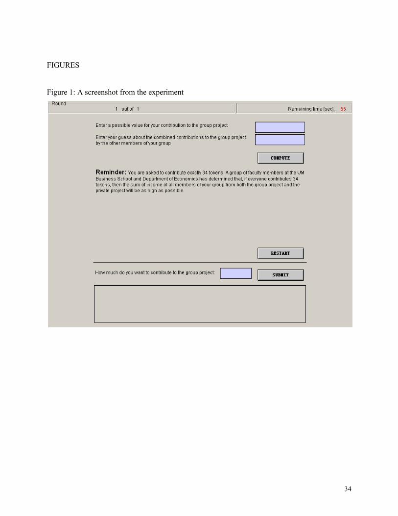
One novelty of our design is that production function for the group project was not
explicitly provided to the subjects. Instead, they were provided with a “calculator” screen that
revealed the income from the group project upon entering two numbers: (1) one’s own
contribution to the group project, and (2) a guess about what the other members of the group will
contribute.7 The calculator added these two values to get the total group contribution and
calculate the subject’s income from the group project. Subjects were able to use the calculator as
many times as they wanted to before they decided how much to contribute to the group project.
Thus they could, in principle, solve for the Nash equilibrium.8 The main reason that we used
non-linear returns and chose not to provide direct information about the payoff structure is to
make the socially efficient level of contributions less obvious to the subjects, and therefore to
make subjects potentially more sensitive to the information provided. This is important because
we examine whether expertise and the source of expertise matters for subjects’ contributions.
2.2.1. The baseline control treatment
In the baseline control treatment, we asked subjects to decide how much to contribute to
the group project, making it a voluntary (non-linear) public good game.
To summarize, in the baseline set-up each subject earned
. The Nash equilibrium has each subject contribute zero to the group project. On the other hand,
the socially optimal level of the group project is the level of contribution that maximizes the joint 7 The calculator screen also contained a reminder of the treatment details. 8 Even though we do not expect that subjects try out all the possibilities, it is straightforward for them to see that, given the contributions of the others in their group, contributing more to the group project always decreases one’s own payoff.
it
210(100 ) 8 0.02i it T Tπ = − + −

7
payoffs. In particular, at the social optimum, total contributions are 137.5. To achieve that level,
each subject would have to contribute approximately 34 tokens.
2.2.2. Treatments examining the effect of authority “in”
We designed all of the treatments such that the Nash equilibrium and the socially optimal
level of contributions do not change.
In the second treatment (denoted NOEXP), the experimenter asked subjects to contribute
the socially optimal amount, but did not provide any explanation. The only difference in the
instructions is the addition of the following sentence:
“In each period, even though you can contribute any amount of your endowment to the
group project, you are asked to contribute exactly 34% of your endowment (34 tokens).”
In the third treatment (EXP), the experimenter asked subjects to contribute the socially
optimal level, and explained that this is the efficient outcome. The previous sentence was
replaced by the following paragraph:
“In each period, even though you can contribute any amount of your endowment to the
group project, you are asked to contribute exactly 34% of your endowment (34 tokens). If
everyone contributes 34 tokens, then the sum of income of all members of your group from the
group project and the private project will be as high as possible.”
In the next set of treatments we investigated the effect of providing different forms of
expert advice, so as to provide evidence about the effect of the authority “in” on contributions.
For the fourth treatment (GRAD_EXP), we explained that a group of experts, graduate students
in economics, had verified that equal contributions of 34 tokens would in fact maximize the sum
of all members’ payoffs.9 The precise language was:
“In each period, even though you can contribute any amount of your endowment to the
group project, you are asked to contribute exactly 34% of your endowment (34 tokens). A group
of graduate students at the UM Department of Economics has determined that, if everyone
contributes 34 tokens, then the sum of income of all members of your group from the group
project and the private project will be as high as possible. You have been provided with an
information sheet that lists the names of these graduate students and a summary of their
achievements.”
9 This was not a deceit. In fact four University of Michigan economics graduate students made this calculation.
8
The fifth treatment (FAC_EXP) was exactly the same as the previous treatment, except
that the expert panel consisted of four economics faculty members instead of graduate students.10
The precise language was:
“In each period, even though you can contribute any amount of your endowment to the
group project, you are asked to contribute exactly 34% of your endowment (34 tokens). A group
of faculty members at the UM Department of Economics has determined that, if everyone
contributes 34 tokens, then the sum of income of all members of your group from the group
project and the private project will be as high as possible. You have been provided with an
information sheet that lists the names of these faculty members and a summary of their
achievements.”
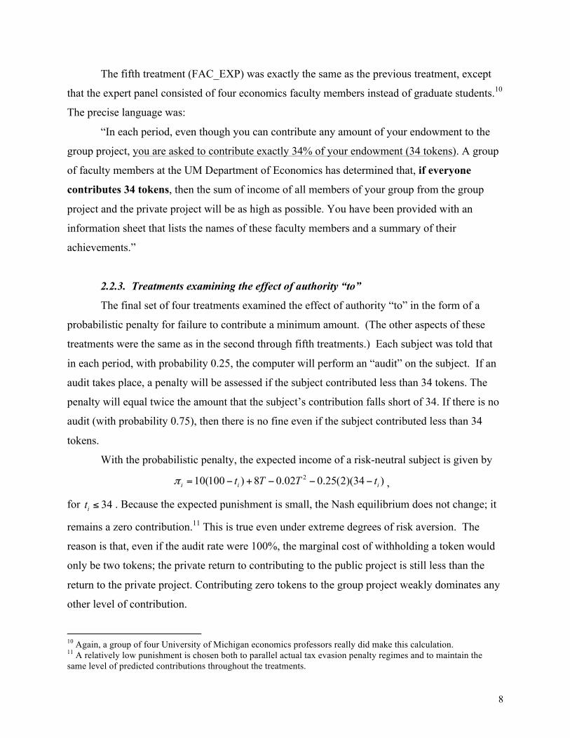
2.2.3. Treatments examining the effect of authority “to”
The final set of four treatments examined the effect of authority “to” in the form of a
probabilistic penalty for failure to contribute a minimum amount. (The other aspects of these
treatments were the same as in the second through fifth treatments.) Each subject was told that
in each period, with probability 0.25, the computer will perform an “audit” on the subject. If an
audit takes place, a penalty will be assessed if the subject contributed less than 34 tokens. The
penalty will equal twice the amount that the subject’s contribution falls short of 34. If there is no
audit (with probability 0.75), then there is no fine even if the subject contributed less than 34
tokens.
With the probabilistic penalty, the expected income of a risk-neutral subject is given by
,
for . Because the expected punishment is small, the Nash equilibrium does not change; it
remains a zero contribution.11 This is true even under extreme degrees of risk aversion. The
reason is that, even if the audit rate were 100%, the marginal cost of withholding a token would
only be two tokens; the private return to contributing to the public project is still less than the
return to the private project. Contributing zero tokens to the group project weakly dominates any
other level of contribution.
10 Again, a group of four University of Michigan economics professors really did make this calculation. 11 A relatively low punishment is chosen both to parallel actual tax evasion penalty regimes and to maintain the same level of predicted contributions throughout the treatments.
210(100 ) 8 0.02 0.25(2)(34 )i i it T T tπ = − + − − −
34it ≤

9
A summary of the experimental design is provided in Table 1. Figure 1 shows a typical
screenshot from the experiment.
Table 1.
Treatment Number of sessions
Number of subjects
(Audit probability; penalty rate)
Level of expertise
BASELINE 3 44 - No suggested level
NOEXP 3 48 - Suggestion w/o explanation
EXP 3 40 - Suggestion with explanation
GRADEXP 3 44 - Suggestion with grad
FACEXP 3 48 - Suggestion with faculty
PEN_NOEXP 3 44 (0.25; 2) Suggestion w/o explanation
PEN_EXP 3 48 (0.25; 2) Suggestion with explanation
PEN_GRADEXP 3 48 (0.25; 2) Suggestion with grad
PEN_FACEXP 3 48 (0.25; 2) Suggestion with faculty
2.2.4. Attitudes and demographic information
Parts 2 and 3 were designed to collect information about the subjects’ risk aversion,
social preferences, attitudes toward taxes and government, and demographic attributes. We will
use these measures as covariates in the analysis of the experimental results. In Part 2, subjects
were asked to perform two separate activities.12 The first activity, designed to obtain information
about risk preferences, asked subjects to choose from among five gambles. The first gamble was
degenerate – it paid 200 tokens with certainty. The remaining four gambles involved a 50-50
chance of receiving either a small or a large amount. The expected value of these gambles
increased – with the smaller amount decreasing and the larger increasing -- up to Gamble 5. That
12 The subjects did not yet know their earnings from Part 1 when they performed these activities.

10
gamble involved the greatest risk and the highest expected value (it paid 600 tokens with
probability 0.5 and nothing otherwise).13
In the second activity of Part 2, subjects were randomly matched with another participant
and had to decide between the three following options that vary a dimension of social
preferences—the tradeoff between one’s own payoff and the sum of payoffs to oneself and
another subject:14
1. You will receive 200 tokens and your paired participant will receive 200 tokens.
2. You will receive 175 tokens and your paired participant will receive 300 tokens.
3. You will receive 225 tokens and your paired participant will receive 100 tokens.
We classify the subjects who picked Option 1 as the “fair,” Option 2 as the “efficiency
maximizer,” and Option 3 as the “selfish/rational.”
In Part 3 we asked the subjects their gender, age, undergraduate major, as well as two
other questions which measure tax morale and trust for public officials. In particular, subjects
were asked whether they agree with the following statements: (1) cheating on taxes, if you have
the chance, can never be justified (tax morale), and (2) public officials can usually be trusted to
do what's right (trust in public officials). These two questions were adapted from similar
questions asked in the World Values Survey.
3. Tabular Results
Table 2 shows the mean contribution levels (and standard deviations15) for each of the
nine treatments, averaged first over all periods and then separately for the first five and last five
periods.
3.1. The effect of suggestion
In all of the treatments, the median contribution is significantly greater than the Nash
equilibrium of zero (p-values < 0.06).16 This is true even in the BASELINE treatment, when no
13 We thus use an ordered lottery selection design in ranking subjects with respect to their risk preferences. See Harrison and Rutström (2008) for a detailed discussion of this and other risk elicitation procedures. 14 The computer randomly chooses one of the participants with equal odds, and implements her decision. 15 Standard deviations are calculated using all observations (not averages over sessions) to show the variations across individuals and periods. Later, when we do statistical testing, we average contributions over sessions to create independent observations.

11
suggested contribution is mentioned.17 However, by far the lowest mean contribution occurs
when the subjects are given no suggestion about how much to contribute, 10.10 tokens
contributed compared to a minimum of 12.15 in the other eight treatments. Comparing the
baseline treatment with NOEXP, we see that the contributions increase by approximately 35%.
This is illustrated in Figure 2. Except for FACEXP, contributions are significantly higher than in
the BASELINE treatment; p-values are less than 0.06 for all comparisons, except for FACEXP,
when it equals 0.26.
The data in Table 3 indicate that the suggestion is, in fact, focal for some subjects. When
contributing exactly 34 tokens is not mentioned (BASELINE), essentially no one contributes
exactly that amount. Over all the other treatments, however, when a 34-token contribution is
mentioned, approximately 19% of period contributions are exactly 34. Notably, suggesting a 34-
token contribution also reduces the fraction of periods in which more than 34 tokens are
contributed, compared to all treatments except the one where no explanation at all is offered
(NOEXP).
Table 4 shows the fraction of individual contributions that equal zero. Note that the
fraction of zero contributions is not tightly correlated with mean contributions. For example, the
treatment with the highest mean contribution (PEN_EXP) also has one of the highest fractions of
periods with zero contributions. This is consistent with the fact that this treatment has the largest
variation of contributions.
3.2. The effect of providing a social-benefit explanation
We have learned that suggesting this contribution level increases contributions. What
about providing an explanation for that suggestion, in particular an explanation about the
potential benefits of widespread contributions to the public good? Here the results are
surprising. A social-benefit explanation increases the mean contribution by 2.70 (p-value = 0.06)
compared to the case where there is a suggestion but no explanation (treatment NOEXP), but
only when it is offered in the context of a penalty regime (Table 2). Contributions to the public
good increase approximately 50% with an explanation and penalty compared to the BASELINE 16 Unless otherwise mentioned, all tests are one-tailed Wilcoxon tests. Note that nonparametric analysis requires independent observations. Therefore, we average contributions over sessions to create independent observations per treatment. 17 Our findings in the baseline treatment are in line with most other non-linear public goods experiments. Laury and Holt (2008) provide a discussion of public goods experiments with a non-linear design.

12
treatment (see Figure 3). In contrast, a social-benefit explanation without a penalty is
accompanied by a decrease in mean contributions of 0.43. The difference is largely due to the
fact that, without a penalty, the explanation prompts a substantial increase in the fraction of zero
contributions, from .28 to .37, especially in the last five periods, where the fraction of zeros goes
from .35 to .50, the highest of any treatment. This is somewhat offset by an increase in the
fraction of those contributing exactly 34, from .14 to .19. With the penalty, though, there is a
slight decrease in the fraction of zero contributions, from .36 to .35, and a decrease in zero
contributions in the last five periods, from .46 to .40. This is the first indication that, in these
settings, authority “in” and authority “to” have important interactive effects.
Figure 3 reveals another interesting finding. In the PEN_EXP treatment, contributions do
not decay over periods nearly as much as in the other treatments.18 While in this and many other
experiments on public goods it is common to observe a decline in contributions over periods, it is
noteworthy that the interaction of authority in and authority to is strong enough to prevent
contributions from substantially declining over periods.
3.3. The effect of authority “in”: Outside expert corroboration
In our research design, the authority “in” aspect of government authority is captured by
two versions of expertise about the social benefit of group-wide contributions to the public
project. We envisioned these two versions, corroboration of the social benefit by graduate
students and by faculty—as steps toward more expertise.
The results do not support the hypothesis that authority “in” or expertise increases
contributions. Nor do they support that student subjects are more influenced to contribute by
faculty, rather than graduate student, corroboration of the social benefit of widespread
contribution. In the no-penalty regimes, comparing the results of EXP to the GRADEXP
treatments shows that graduate student expertise increases mean contributions by just 0.02.
Comparing EXP to FACEXP shows that faculty corroboration of the social benefit actually
decreases contributions by 0.98. However, none of the pairwise comparisons between EXP,
GRADEXP, and FACEXP is statistically different from zero (the p-values are all larger than
0.26). These patterns may in part be explained by student subject suspicions about the expertise,
18 This finding is supported by a regression analysis. When contributions are regressed on period, we find a p-value of 0.26 for this particular treatment.

13
or motivation, of faculty “experts.”19 It also may be that the “unattributed” explanation is in fact
attributed to the experimenter who, as already discussed, is a kind of authority figure herself.
Finally, a suggestion in and of itself may convey expertise.20
In addition, in the penalty regimes neither kind of expert testimony increases
contributions. Graduate student expertise decreases contributions by 1.71, and faculty expertise
reduces contributions by 1.34. Similarly, none of the pairwise comparisons is statistically
distinguishable from zero (the smallest p-value is 0.14).
3.4. The effect of authority “to”: Penalties
Adding a probabilistic penalty for contributing less than the socially efficient amount
increases the expected private return to contributing, although it does not budge Nash
equilibrium behavior from a zero contribution. We can get a sense of the effect on contributions
of a penalty by comparing the contribution pattern for each setting of explanation/expertise, that
is comparing the results in NOEXP to PEN_NOEXP, EXP to PEN_EXP, GRADEXP to
PEN_GRADEXP, and FACEXP to PEN_FACEXP.
The results suggest that the impact of authority “to” depends on the extent of authority
“in.” When no explanation is offered for the suggested contribution, adding a penalty decreases
mean contributions by 0.48. However, the difference is not significantly distinguishable from
zero (p-value = 0.41). In contrast, when the suggestion is accompanied by an explanation,
adding a penalty (insignificantly) increases mean contributions, by 2.65, 0.92, and 2.19 for the
three treatments with explanations (p-values > 0.14). An interesting finding is that, even though a
penalty doesn’t affect the contributions significantly when all periods are considered, adding a
penalty increases contributions significantly between treatments EXP and PEN_EXP, and
treatments GRADEXP and PEN_GRADEXP (p-values = 0.02) when attention is restricted to
just the last 5 periods.
19 While our statements regarding the experts were completely accurate, it is also possible that some students viewed it as implausible that so much faculty or graduate student time would have been devoted to calculating the social optimum for the experiment. 20 It has been suggested to us that referring to economics faculty or graduate students might change the subjects’ framing of the experiment—they now realize it is an “economics” experiment. This seems unlikely because the economics background of the experimenters was indicated in the consent form and in the background remarks communicated at the outset of the experiment.

14
3.5. Varying Gradient
As the second and third columns of Table 2 show, for nearly all treatments there is a
significant drop-off in mean contributions between the first 5 periods and the last 5 periods (all
p-values < 0.06, except for PEN_EXP, which is 0.26).21 But the drop-off varies substantially
across treatments, both in absolute and in percentage terms. Thus the treatments do not simply
affect the initial contribution levels, with a uniform dilution over time, but affect both the initial
levels and the gradients.
The lowest beginning-to-end drop-off in contributions comes in the PEN_EXP treatment,
where the drop-off is only 2.28.22 Table 4 shows that, for all of the treatments, the fraction of the
contributed amounts that are exactly zero increases between the first and last five periods. There
is a clear positive correlation across treatments between the decline in mean contributions and
the increase in the fraction of zero contributions. Both are smallest for the PEN_EXP treatment.
One possible explanation for why we do not observe lower drop-off in the expert advice
treatments is that, in these treatments, subjects feel a sense of betrayal that the advice offered has
failed to be helpful (or even relevant, given that most of their group members are not
contributing large amounts). They react in an anti-social way more so than they do when the
advice is offered in an impersonal way (by the experimenter, without attribution to particular
“expert” individuals), because the impersonal process does not trigger the feelings of
intentionality and reciprocity that the advice linked to real people does. People react differently
to the same behavior of a person and an impersonal actor, as Blount (1995) suggested.
4. Regression Analysis
With multivariate regression analysis we can explore more precisely the interaction
effects of the treatment elements and also investigate the relationship to contribution decisions of
subject attributes and attitudes. In all of the results, we report robust standard errors clustered at
the session level.
21 This decline in average giving is the subject of a large literature in its own right. See Fischbacher and Gachter (2010) for a recent contribution and review. 22 All pairwise comparisons (with the exception of the first treatment) are significantly different, with p-values equal to or less than 0.06.

15
We begin in Table 5 with an OLS regression that includes all period observations. In this
and subsequent tables the variable suggestion takes a value of 0 for no suggested level of tax, and
1 otherwise, so that suggestion equals 0 only for treatment BASELINE. The variable
explanation takes the value 1 if the treatment is either EXP or PEN_EXP, so that it refers to an
explanation without expert corroboration. The variables grad expert and faculty expert are
indicator variables equal to one when there is graduate student corroboration and faculty
corroboration, respectively. The variable penalty takes the value 0 when there is no fine and a
value of 1 when there is a fine. The variable period takes values from 1 to 20.23 The variable
gamble takes values from 1 to 5, where 1 corresponds to the riskless lottery and 5 corresponds to
the riskiest lottery. The variable fair takes a value of 1 if a subject chooses the fair option in
activity 2 of Part 2, and a value of 0 otherwise. The variable efficiency takes a value of 1 if a
subject chooses the “efficiency maximizer” option in activity 2 of Part 2, and value of 0
otherwise. The variable age is simply the age of the subject. The variable female takes a value of
1 if the subject is female and 0 otherwise. The variable econ takes a value of 1 if the subject is an
economics major and 0 otherwise. The variable taxmorale takes values from 1 to 7, where 1
means that a subject “completely disagrees” that cheating on taxes can never be justified, and 7
implies that a subject “completely agrees” with that statement. The variable trustinpublicofficials
also takes values 1 to 7 where 1 implies that a subject “completely disagrees” that public officials
can usually be trusted to do what's right, and 7 implies that a subject “completely agrees” with
that statement.
In specification (1) of Table 5, only suggestion significantly affects contributions,
increasing contributions by 2.64. This is consistent with the tabulated results discussed earlier.
Specification (2) shows that each of the three attitudinal variables gamble, fair, and efficiency is
significantly associated with contributions in the expected direction. The estimated coefficient
on the variable gamble has a negative sign and is marginally significant, though the degree of
risk aversion should not affect contributions in our experiment. In contrast, the estimated
coefficients of fair and efficiency are large, positive, and highly significant; these effects are
relative to selfish subjects. These results are consistent with the existing experimental literature,
23 As a robustness check, we also investigated a specification that allowed for a non-linear learning process, with no qualitative difference in the results reported here.

16
which documents that people with fairness or efficiency concerns would give up their own
earnings in order to help others.24
Also, as expected, due to the random assignment of subjects to treatment, adding the
attitudinal variables as explanatory variables does not greatly change the other estimated
coefficients. Neither taxmorale nor trustinpublicofficials has a significant partial association
with the level of contributions.25 Of the three demographic variables, only female affects the
magnitude of contributions in a statistically significant way, and does so positively. Two aspects
of the main results change when the whole set of explanatory variables is included. First the
explanation variable now attracts a significant positive coefficient. Second, the negative
estimated coefficient on gamble just fails the test for statistical significance, presumably because
there is correlation between it and the newly included explanatory variables. In all
specifications, the estimated coefficients on the period variable suggest a substantial downward
drift over time in the level of contributions.
The regression specifications shown in Table 6 add interaction terms of the penalty
treatment with the three expertise treatments. They show that the combination of an explanation
and a penalty increases contributions, but neither by itself. Notably, this interaction effect is
least strong when the explanation is backed up by graduate student or faculty corroboration, but
is quantitatively significant (a coefficient in excess of three), and is statistically different than
zero whenever the non-treatment explanatory variables are included in the regression
specification. Now we see that having a penalty increases contributions only in conjunction with
an explanation, and especially so when there is an explanation without supporting expertise.26
Tables 7 and 8 repeat the specifications with interactions effects for contributions in the
first five and last five periods, respectively. Comparing the results of these two sets of
regressions reveals that the positive effect on contributions of making a suggestion fades away
over time, being associated with about five more tokens in the early period but only about half of
that by the end. In contrast, the impact of the combination of an explanation and a penalty is
stronger near the end of the experiment’s duration than at the beginning. In specification (3) of
Table 8, explanation has a positive effect of 1.4, but combined with a penalty, the explanation is 24 See, for example, Andreoni (2006), Camerer (2003), Charness and Rabin (2002), and, Fehr and Schmidt (2006). 25 This result is not particularly surprising considering that the transfers in the experiment are not between the subject and a government authority or public officials. 26 We have also estimated a Tobit regression specification. The qualitative results do not change, with the exception that the variable gamble now significantly affects contributions.

17
associated with 6.6 more contributions. Of particular interest is the time pattern of the estimated
effect of authority “in.” In the last five periods, but not in the initial five periods, both the
graduate-student and faculty corroboration reduce contributions, absent a penalty (the former
being statistically different from zero). In the faculty case, the effect essentially goes to zero
when combined with a penalty, but the graduate-student explanation with a penalty increases
contributions at the end.
Table 9 pursues the extensive effect on contributions with the results of a linear
probability model of contributing any positive amount. It confirms that female subjects are more
likely to give a positive amount.27 The penalty reduces the probability of contributing any
positive amount.
5. Discussion
In these experiments, simply asking subjects to contribute to a public project increased
their contributions by over a third, even though their private self-interest dictated that they
contribute nothing. This is consistent with the view that is relatively easy for authorities to
increase the frequency or level at which people deviate from their material self-interest. But
why? A subject might be trying to please the experimenter, either because she is herself a figure
of authority or because she has kindly offered compensation and otherwise been courteous, so
that the pro-social behavior is a kind of reciprocity. Alternatively, subjects may respond to a
suggested level of contribution because they believe it is good advice that, if followed, will
improve their outcome. The experimenter “knows” something that the subject does not. Finally,
a subject may contribute when there is a penalty for not doing so, either because of how this
changes the material incentives or because it conjures up something about the social value of
contributing; this is the authority “to” punish non-compliers. In addition, we might imagine that
the suggestion of a particular contribution level facilitates, at least temporarily, coordination on a
group equilibrium with higher contributions and better outcomes for all subjects.
Our experimental treatments do not provide much evidence that subjects increase their
contributions in order to improve their outcomes. Merely providing a social-benefit explanation
for a contribution does not increase contributions. Nor does buttressing the explanation with 27 However, this does not mean that females give more conditional on giving anything. The average contribution of female subjects is 14.7, while the average contribution of male subjects is 11.8. However, when we only look at contributions that are positive, male subjects contribute 20.9 on average, while female subjects contribute 19.1.

18
testimony from apparent experts other than the experimenter herself—economics graduate
students and faculty. Indeed, expertise on its own seems to crowd contributions out a bit, the
more so the greater the apparent expertise.28
Nor do we find evidence that penalties themselves induce more pro-social contributions.
Indeed, penalties for contributions below the socially efficient level generally seem to decrease
contributions slightly.
What we do find is that the combination of authority “in” and authority “to” increases
contributions. To our knowledge, this is the first laboratory experiment demonstration of this
interactive effect. An explanation that widespread contributions to the public project can improve
everyone’s outcome, when coupled with a penalty for less-than-socially optimal contributions, is
successful in raising contributions, and results in an average level of contribution that exceeds
the average in all the other treatments we administered.
The reinforcing effect of authority “in” and authority ‘to” may be interpreted as a
legitimacy effect. Subjects for whom penalties may otherwise reduce contributions, whether
because of motivational crowd out (i.e., moving from intrinsic to extrinsic motivation) or a
“hidden cost of control,”29 are less likely to react this way when there is a good reason for the
penalty (it supports a socially efficient level of the public project). The same results can also be
interpreted as evidence of a different kind of legitimacy effect, in which the imposition of
penalties provides support for the offered explanation for contributing to the public project: “we
think the advice is good enough that we are willing to penalize those that don’t follow it.” This
works to counteract the otherwise negative consequences of offered expertise that we have found
in this experiment. This finding is consistent with the view argued compellingly by Tyler (2006)
that people are more likely to obey rules, including but not limited to penalties, if those rules
seem fair (right) and legitimate. Finally, it may be that combining an explanation with a
potential penalty transforms asking for a contribution into something that is perceived as
approaching an obligation; future research might explore how the effects of explanation and
penalty affect behavior when compliance is required rather than suggested.
28 As Christian Traxler noted to us, at the time of the experiments--in the aftermath of the financial crisis and recession-- many people may not have been inclined to think of economists as “experts” on much of anything. We note, though, that the issue in question in the experiment is far removed from these macroeconomic events. 29 See Falk and Kosfeld (2006).

19
It may also be that offering expert advice triggers a kind of motivational crowding out
similar to what is triggered in other contexts by monetizing pro-social behavior. The argument
goes as follows: offering a selfish reason for contributions (“if everyone does it, you’ll be better
off”) causes some people to switch their mental framing of the contribution decision from a pro-
social to a selfish one.
We find that merely suggesting a level of contribution level, with no explanation or
penalty, significantly increases contributions, suggesting that minimal intervention can affect
voluntary socially efficient behavior. But, beyond that, when we consider providing outside
expert justification for the requested level of contribution or assessing penalties for contributions
below that level, neither on its own is successful, but only the combination of an expert
explanation plus sanctioning works.
6. Related Literatures
As a laboratory study of voluntary contributions to a public good, this paper relates to a
large experimental literature concerned with this canonical economic problem.30 By requesting
that subjects give a particular contribution, and sometimes penalizing their failure to comply with
this request, the paper also relates to substantial literature on tax compliance games.31
As noted above, there is a substantial psychology literature on authority and obedience.32
However, both the economics of voluntary contributions to public goods and the experimental
literature on tax compliance largely ignore the role of authority. An exception is Cadsby et al.
(2006), who study the consequences of an explicit demand of compliance in a tax evasion
experiment. In particular, Cadsby et al. investigate the effects of describing compliance with a
tax scheme as a requirement, not merely as the way to avoid a probabilistic penalty. Our
baseline results are similar to theirs, in that we find important effects of a request to give at a
30 Ledyard (1995) reviews the early literature, and Andreoni et al. (2008) summarizes some of the more recent studies. 31 Torgler (2002) and Alm and Jacobson (2007) review much of this literature. Our penalty treatments are especially close to the public goods experiments on “mild laws.” Feld and Tyran (2006), Galbiati and Vertova (2008), and Kube and Traxler (forthcoming) all study the effects of random auditing with non-deterrent sanctions. In these experiments, like ours, the expected penalties are so small that they should have no deterrent effect on rational players. These papers also find effects of such penalties. 32 Cialdini and Goldstein (2004) provide an excellent review. There is some, qualitative, evidence in this literature to indicate that authority in and authority to may have complimentary effects on behavior.

20
certain level.33 Our work is distinct, however, in that we build on this finding in an attempt to
understand better why the simple request to comply is effective by exploring the role of, and
interaction among, providing an explanation (sometimes provided by an expert) and a penalty for
contributions less than the suggested amount. In particular, our efforts to distinguish the role of
authority “in” and authority “to,” and to understand their complementarities, are, to our
knowledge, the first of their kind.34
As we study the role of authority “in,” our paper also relates to an experimental literature
concerned with the effects of advice on equilibrium play. Schotter and Sopher (2003, 2007)
study inter-generational games in which advice can be passed from outgoing to incoming players
via free-form messages. Importantly, the only source of authority for these outgoing players is
their brief, previous experience. These experiments suggest that even non-expert advice can have
a significant impact on decisions. Chaudhuri, Graziano, and Maitra (2006) show that advice in
the form of common knowledge (i.e., publicly announced to all members of the group) is most
successful at increasing contributions, which they argue is because it facilitates successful
socially efficient high levels of contributions. To our knowledge, the role of outside expert
advice, and its quality, has not yet been studied in public-good games.
Finally, as we study the interactions between simple requests and requests backed by material
penalties, our paper relates to a literature on the crowd-out of intrinsic motivation by extrinsic
incentives. Frey (1997), for example, differentiates between intrinsic motivation under which
taxpayers comply with tax liabilities because of “civic virtue” and extrinsic motivation in which
they pay because of threat of punishment, and suggests that increasing extrinsic motivation may
“crowd out” intrinsic motivation by making people feel that they pay taxes because they have to,
rather than because they want to. Gneezy and Rustichini (2000) argue that this explains why
parent tardiness increased after an Israeli day care center instituted monetary fines for late pick-
up of children. Similarly, Scholz and Lubell (2001) find that the level of cooperation in certain
settings declines significantly when penalties are introduced; and Falk and Kosfeld (2006) find
33 We did not study the potentially interesting distinctions between requests and demands for compliance. 34 These aspects of our study also distinguish it from others that find important effects of requests or recommendations. Marks et al. (1999) and Chaudhuri and Paichayontvijit (2010), for examples, study the effects of the experimenter’s recommendation, or offer of additional incentive, to coordinate at the socially optimal level in a minimum effort game; and Andreoni and Rao (2011) show that the communication of simple requests can dramatically influence altruistic behavior in lab experiments. Pointing in the opposite direction, Dale and Morgan (2010) show that suggesting contribution levels depresses average giving in the lab.

21
“hidden costs of control” -- implementing a minimum performance requirement causes most
agents to reduce their overall performance in response. Our paper contributes to this literature by
identifying, to our knowledge for the first time, complementarities between intrinsic and
extrinsic motivations.
7. Conclusion
Governments can provide value by mobilizing resources to provide public goods, and can
use their coercive power to enforce tax remittances from citizens who would prefer to be free
riders. Governments often also have an information advantage regarding which activities would
benefit citizens. They have the authority “to” enforce the law, including their tax law, and
authority “in” the provision of public goods.
History shows clearly, however, that not all governments act in the interest of all citizens,
and therefore many citizens are suspicious of the information that government provides to justify
its actions and are resentful of the powers it uses to enforce tax obligations. Pleas to comply for
the social good often go unheeded, and heavy-handed enforcement can often backfire.
The results of the experiments described in this paper suggest that authority “to” and
authority “in” interact in ways not heretofore understood. Coercion without explanation does not
increase voluntary contributions, nor does explanation without coercion. Together, they induce
more contributions than any other combination of policies. In our interpretation, this reveals that
how people react to authority depends on whether this authority is perceived to be legitimate.

22
References
Alm, James and Sarah Jacobson. 2007. “Using lab experiments in public economics.” National
Tax Journal 60: 129-152.
Andreoni, James. 2006. “Philanthropy.” In S. Kolm and Jean Mercier Ythier (eds.), Handbook
of Giving, Reciprocity and Altruism. Amsterdam: North Holland: 1201-1269.
Andreoni, James and Justin M. Rao. 2011. “The power of asking: How communication affects
selfishness, empathy, and altruism.” Journal of Public Economics 95(7-8): 513-520.
Andreoni, James, William T. Harbaugh, and Lise Vesterlund. 2008. “Altruism in experiments.”
In Steven Durlauf and Lawrence E. Blume (eds.), The New Palgrave Dictionary of Economics,
2nd Edition. Basingstoke, UK: Palgrave Macmillan
Andreoni, James and Lise Vesterlund. 2001. “Which is the fair sex? Gender differences in
altruism.” The Quarterly Journal of Economics 116(1): 293-312.
Bernheim, B. Douglas and Daniel M. Garret. 2003. “The effects of financial education in the
workplace: Evidence from a survey of households.” Journal of Public Economics 87(7-8): 1487-
1519.
Beshears, John, James J. Choi, David Laibson, and Brigitte C. Madrian. 2009. “The importance
of default options for retirement savings outcomes: Evidence from the United States.” In Jeffrey
R. Brown, Jeffrey B. Liebman, and David A. Wise (eds.), Social Security Policy in a Changing
Environment. Chicago and London: The University of Chicago Press and NBER.
Blount, Sally. 1995. “When social outcomes aren't fair: The effect of causal attributions on
preferences.” Organizational Behavior and Human Decision Processes 63: 131-144.
23
Cadsby, C. Bram, Elizabeth Maynes, and Visawanath Umashanker Trivedi. 2006. “Tax
compliance and obedience to authority at home and in the lab: A new experimental approach.”
Experimental Economics 9: 343-359.
Camerer, Colin. 2002. Behavioral Game Theory. Princeton, NJ: Princeton University Press.
Charness, Gary and Matthew Rabin. 2002. “Understanding social preferences with simple tests.”
The Quarterly Journal of Economics 117: 817–869.
Chaudhuri, Ananish, Sara Graziano, and Pushkar Maitra. 2006. “Social learning and norms in a
public goods experiment with intergenerational advice.” The Review of Economic Studies 73(2):
357-380.
Chaudhuri, Ananish and Tirnud Paichayontvijit. 2010. “Recommended play and performance
bonuses in the minimum effort coordination game.” Experimental Economics vol. 13: 346-363.
Choi, James, David Laibson, Brigitte C. Madrian, and Andrew Metrick. 2004. “For better or
for worse: Default effects and 401(k) savings behavior.” In Perspectives in the Economics of
Aging, David A. Wise (ed.). Chicago: University of Chicago Press.
Cialdini, Robert B. and Noah J. Goldstein 2004. “Social influence: Compliance and conformity.”
Annual Review of Psychology 55: 591-621.
Dale, Donald and John Morgan. 2010. “Silence is golden: Suggested donations in voluntary
contribution games.” Mimeo, University of California – Berkeley.
Falk, Armin and Michael Kosfeld. 2006. “The hidden costs of control.” American Economic
Review 96(5): 1611-1630.

24
Fehr, Ernst and Klaus M. Schmidt. 2006. "The economics of fairness, reciprocity and altruism:
Experimental evidence and new theories." In S. Kolm and Jean Mercier Ythier (eds.), Handbook
of Giving, Reciprocity and Altruism. Amsterdam: North Holland: 615-691.
Feld, Lars P. and Bruno S. Frey. 2002. “Trust breed trust: How taxpayers are treated.”
Economics of Governance 3: 87-99.
Fischbacher, Urs. 2007. “z-Tree: Zurich toolbox for ready-made economic experiments.”
Experimental Economics 10(2): 171-178.
Fischbacher, Urs. And Simon Gächter. 2010. “Social preferences, beliefs, and the dynamics of
free riding in public goods experiments.” American Economic Review 100(1): 541-56.
Galbiati, Roberto and Pietro Vertova (2008), “Obligations and cooperative behaviour in public
good games.” Games and Economic Behavior 64(1): 146-170.
Gneezy, Uri and Aldo Rustichini. 2000. “A fine is a price.” Journal of Legal Studies 29: 1-17.
Harrison, G.W. and Elisabet Rutström. 2008. "Risk aversion in the laboratory," in J.C. Cox and
G.W. Harrison (eds.), Risk Aversion in Experiments. Research in Experimental Economics,
Volume 12. Bingley, UK: Emerald.
Kube, Sebastian and Christian Traxler. 2011. “The interaction of legal and social norm
enforcement.” Journal of Public Economic Theory 13(5): 639-660.
Laury, Susan K. and Holt, Charles A., 2008. “Voluntary provision of public goods: Experimental
results with interior Nash equilibria.” In Charles R. Plott and Vernon L. Smith (eds.), The
Handbook of Experimental Economics Results: 792-801. Elsevier,
http://econpapers.repec.org/RePEc:eee:expchp:6-84.
Levitt, Steven and John List. 2007. “What do laboratory experiments measuring social
preferences reveal about the real world?” The Journal of Economic Perspectives 21: 153-174.

25
Ledyard, J. O. 1995. “Public goods: A survey of experimental research.” In J. H. Kagel and A. E
Roth (eds.), The Handbook of Experimental Economics. Princeton: Princeton University Press.
Lusardi, Annamaria and Olivia S. Mitchell. 2007. “Financial literacy and retirement
preparedness: Evidence and implications for financial education.” Business Economics 42(1):
35-44.
Madrian, Brigitte C. and Dennis Shea. 2001. “The power of suggestions: Inertia in 401(k)
participation and saving behavior.” Quarterly Journal of Economics 116(4): 1149-87.
Marks, Melanie B., D. Eric Schansberg, and Rachel T. A. Croson. 1999. “Using Suggested
Contributions in Fundraising for Public Good: An Experimental Investigation of the Provision
Point Mechanism,” Nonprofit Management and Leadership Vol. 9, 369-384.
Martin, Matthew. 2007. “A literature review on the effectiveness of financial education.” The
Federal Reserve Bank of Richmond Working Paper Series 07-3.
Milgram, Stanley. 1974. Obedience to authority. New York, NY: Harper & Row.
Morelli, Mario F. 1983. “Milgram’s dilemma of obedience.” Metaphilosophy 14 (3-4): 183-
189.
Scholz, John T. and Mark Lubell. 2001. “Cooperation, reciprocity, and collective-action
rhetoric.” American Journal of Political Science 45(1): 160-178.
Schotter, Andrew and Barry Sopher. 2003. “Social learning and coordination conventions in
intergenerational games: An experimental study.” Journal of Political Economy 111(3): 498-
529.
Schotter, Andrew and Barry Sopher. 2007. “Advice and behavior in intergenerational
ultimatum games: An experimental approach.” Games and Economic Behavior 58(2): 365-393.

26
Torgler, Benno. 2002. “Speaking to theorists and searching for facts: Tax morale and tax
compliance in experiments.” Journal of Economic Surveys 16(5): 657-683.
Tyler, Tom R. 2006. Why people obey the law. Princeton: Princeton University Press.
Tyran, Jean-Robert and Lars P. Feld. 2006. “Achieving compliance when legal sanctions are
non-deterrent.” The Scandinavian Journal of Economics 108(1): 135-156.
Zizzo, Daniel John. 2010. “Experimenter demand effects in economic experiments.”
Experimental Economics 13(1): 75-98.

27
TABLES Table 2. Mean contribution levels
Treatment Mean Contribution Mean Contribution First 5 periods
Mean Contribution Last 5 Periods
BASELINE 10.10 (14.24)
12.65 (14.82)
7.52 (12.92)
NOEXP 13.56 (15.15)
17.50 (18.05)
10.14 (12.92)
EXP 13.13 (15.40)
16.39 (15.40)
10.82 (16.25)
GRADEXP 13.15 (14.53)
17.90 (16.03)
8.10 (12.52)
FACEXP 12.15 (13.53)
17.23 (14.66)
8.62 (11.98)
PEN_NOEXP 13.08 (15.58)
16.80 (15.17)
9.85 (15.43)
PEN_EXP 15.78 (15.95)
17.30 (15.69)
15.01 (16.98)
PEN_GRADEXP 14.07 (15.34)
17.25 (16.24)
11.19 (14.13)
PEN_FACEXP 14.34 (14.22)
18.97 (15.50)
10.60 (12.75)
Standard deviations in parentheses
Table 3. Proportion of contributions less than, equal to, and above 34
Treatment Less Than 34 Exactly 34 More Than 34 BASELINE 0.94 0.00 0.06 NOEXP 0.80 0.14 0.06 EXP 0.79 0.19 0.02 GRADEXP 0.81 0.17 0.02 FACEXP 0.83 0.15 0.03 PEN_NOEXP 0.78 0.17 0.04 PEN_EXP 0.69 0.27 0.04 PEN_GRADEXP 0.76 0.22 0.02 PEN_FACEXP 0.80 0.19 0.01

28
Table 4. Proportions of observations with contribution exactly equal to 0
Treatment All Periods First 5 periods Last 5 periods
BASELINE 0.34 0.30 0.42
NOEXP 0.28 0.22 0.35
EXP 0.37 0.26 0.50
GRADEXP 0.28 0.20 0.41
FACEXP 0.33 0.26 0.41
PEN_NOEXP 0.36 0.25 0.46
PEN_EXP 0.35 0.31 0.40
PEN_GRADEXP 0.36 0.25 0.44
PEN_FACEXP 0.32 0.23 0.43

29
Table 5. Baseline OLS regressions
DEP. VARIABLE= contribution/tax
suggestion 2.640** 3.080* 3.099** (1.257) (1.499) (1.356) explanation 1.159 1.542 2.067* (1.115) (1.079) (1.131) grad expert 0.248 -0.0329 -0.0929 (0.796) (0.932) (0.993) faculty expert -0.111 -0.649 -0.715 (1.429) (1.135) (1.084) penalty 1.313 1.422 1.163 (0.873) (0.862) (0.869) period -0.453*** -0.453*** -0.453*** (0.0449) (0.0449) (0.0449) gamble -0.853* -0.654 (0.425) (0.443) fair 4.996*** 4.650*** (0.990) (0.947) efficiency 8.878*** 9.301*** (1.859) (1.833) age 0.0119 (0.144) female 2.637** (0.975) econ 1.431 (1.471) taxmorale 0.314 (0.312) trustinpublicofficials 0.479 (0.341) Constant 10.06*** 9.213*** 8.300 (0.898) (1.750) (5.000) Observations 8240 8240 8240 R-squared 0.008 0.057 0.098 *Significant at 10%, **significant at 5%, ***significant at 1% Robust standard errors are in parentheses. (Two tailed-results reported.)

30
Table 6. Including interaction terms
DEP. VARIABLE= contribution/tax
suggestion 3.496** 3.678** 3.966*** (1.389) (1.577) (1.377) explanation -0.425 -0.185 0.0945 (1.636) (1.335) (1.214) grad expert -0.404 -0.169 -0.715 (1.239) (1.226) (1.385) faculty expert -1.405 -1.349 -1.761 (2.098) (1.558) (1.338) penalty -0.478 0.160 -0.662 (1.115) (0.904) (0.645) explanation * penalty 3.125 3.326* 3.861** (1.986) (1.908) (1.863) grad expert * penalty 1.400 0.370 1.338 (1.361) (1.730) (1.781) faculty expert * penalty 2.665 1.449 2.159 (2.713) (2.247) (2.043) period -0.453*** -0.453*** -0.453*** (0.0449) (0.0449) (0.0449) gamble -0.882** -0.678 (0.418) (0.436) fair 4.960*** 4.598*** (0.991) (0.951) efficiency 8.944*** 9.324*** (1.858) (1.829) age 0.0157 (0.145) female 2.699*** (0.960) econ 1.486 (1.473) taxmorale 0.319 (0.311) trustinpublicofficials 0.478 (0.338) Constant 10.06*** 9.325*** 3.503 (0.898) (1.734) (4.730) Observations 8,240 8,240 8,240 R-squared 0.010 0.058 0.069 *Significant at 10%, **significant at 5%, ***significant at 1% Robust standard errors are in parentheses. (Two tailed-results reported.)

31
Table 7. OLS regressions for the first 5 periods
DEP. VARIABLE= contribution/tax
suggestion 4.850** 5.225** 4.952** (2.076) (2.016) (1.973) explanation -1.119 -0.952 -0.462 (1.769) (1.280) (1.157) grad expert 0.400 0.355 0.00192 (1.576) (0.990) (0.774) faculty expert -0.279 -0.429 -0.613 (1.440) (1.317) (1.249) penalty -0.704 -0.191 -1.155 (1.681) (1.780) (1.389) explanation * penalty 1.615 1.881 2.567 (2.197) (2.022) (1.783) grad expert * penalty 0.0538 -0.827 0.204 (2.049) (2.005) (1.579) faculty expert * penalty 2.450 1.243 1.938 (2.879) (2.686) (2.534) period -1.595*** -1.595*** -1.595*** (0.176) (0.176) (0.176) gamble -1.165*** -0.894** (0.413) (0.395) fair 5.711*** 5.011*** (1.107) (1.070) efficiency 8.285*** 8.694*** (1.728) (1.692) age 0.170 (0.195) female 3.495*** (1.025) econ -0.0382 (1.868) taxmorale 0.325 (0.365) trustinpublicofficials 0.577 (0.406) Constant 12.65*** 12.54*** 3.109 (1.777) (2.356) (5.686) Observations 2,060 2,060 2,060 R-squared 0.011 0.061 0.077 *Significant at 10%, **significant at 5%, ***significant at 1% Robust standard errors are in parentheses. (Two tailed-results reported.)

32
Table 8. OLS regressions for the last 5 periods
DEP. VARIABLE= contribution/tax
suggestion 2.615 2.671 2.621 (1.893) (2.190) (1.854) explanation 0.683 0.960 1.352** (1.013) (0.820) (0.641) grad expert -2.042* -1.580* -1.922** (1.150) (0.913) (0.909) faculty expert -1.517 -1.345 -1.594 (2.557) (1.912) (1.681) penalty -0.292 0.482 -0.200 (0.965) (0.993) (0.896) explanation * penalty 4.485** 4.741** 5.239*** (1.659) (1.854) (1.821) grad expert * penalty 3.388** 2.104 2.895** (1.251) (1.390) (1.370) faculty expert * penalty 2.275 0.920 1.394 (3.308) (2.896) (2.718) period -0.664*** -0.664*** -0.664*** (0.166) (0.166) (0.166) gamble -0.960* -0.709 (0.516) (0.536) fair 4.819*** 4.470*** (1.107) (1.085) efficiency 10.48*** 11.03*** (2.103) (2.074) age -0.0377 (0.147) female 3.053** (1.229) econ 0.494 (1.308) taxmorale 0.152 (0.414) trustinpublicofficials 0.314 (0.386) Constant 7.523*** 6.956** 3.699 (1.693) (2.646) (5.634) Observations 2,060 2,060 2,060 R-squared 0.022 0.086 0.098 *Significant at 10%, **significant at 5%, ***significant at 1% Robust standard errors are in parentheses. (Two tailed-results reported.)

33
Table 9. Linear probability model
DEP. VARIABLE= contributed
suggestion 0.064 0.081 0.066 (0.043) (0.053) (0.043) explanation -0.098 -0.098 -0.076 (0.073) (0.082) (0.073) grad expert -0.004 -0.017 -0.029 (0.055) (0.033) (0.017) faculty expert -0.049 -0.063 -0.073** (0.035) (0.037) (0.030) penalty -0.085*** -0.078** -0.114*** (0.026) (0.033) (0.018) explanation * penalty 0.107 0.120 0.150 (0.084) (0.102) (0.094) grad expert * penalty 0.007 -0.012 0.027 (0.072) (0.069) (0.052) faculty expert * penalty 0.088 0.057 0.082 (0.073) (0.064) (0.061) period -0.012*** -0.012*** -0.012*** (0.001) (0.001) (0.001) gamble -0.051*** -0.036** (0.013) (0.013) fair 0.175*** 0.143*** (0.034) (0.032) efficiency 0.193*** 0.222*** (0.065) (0.060) age 0.002 (0.004) female 0.181*** (0.028) econ -0.012 (0.067) taxmorale 0.012 (0.011) trustinpublicofficials 0.007 (0.014) Constant 0.782*** 0.837*** 0.584*** (0.037) (0.067) (0.141) Observations 8,240 8,240 8,240 R-squared 0.025 0.083 0.119 *Significant at 10%, **significant at 5%, ***significant at 1% Robust standard errors are in parentheses. (Two tailed-results reported.)
34
FIGURES
Figure 1: A screenshot from the experiment

35
Figure 2: Mean Contribution to the Public Good: BASELINE versus NOEXP Treatment
Figure 3: Mean Contribution to the Public Good: BASELINE, PEN_NOEXP and PEN_EXP
Treatments
0
5
10
15
20
25
0 5 10 15 20
Mea
n C
ontr
ibut
ion/
Tax
Period
BASELINE NOEXP
0
5
10
15
20
25
0 5 10 15 20
Mea
n C
ontr
ibut
ion/
Tax
Period
BASELINE PEN_NOEXP PEN_EXP