Embed Size (px)
Citation preview

Author's Accepted Manuscript
Sub-pixel Mapping Based on Artificial Im-mune Systems for Remote Sensing Imagery
Yanfei Zhong, Liangpei Zhang
PII: S0031-3203(13)00179-9DOI: http://dx.doi.org/10.1016/j.patcog.2013.04.009Reference: PR4782
To appear in: Pattern Recognition
Received date: 4 June 2012Revised date: 8 April 2013Accepted date: 13 April 2013
Cite this article as: Yanfei Zhong, Liangpei Zhang, Sub-pixel Mapping Based onArtificial Immune Systems for Remote Sensing Imagery, Pattern Recognition,http://dx.doi.org/10.1016/j.patcog.2013.04.009
This is a PDF file of an unedited manuscript that has been accepted forpublication. As a service to our customers we are providing this early version ofthe manuscript. The manuscript will undergo copyediting, typesetting, andreview of the resulting galley proof before it is published in its final citable form.Please note that during the production process errors may be discovered whichcould affect the content, and all legal disclaimers that apply to the journalpertain.
www.elsevier.com/locate/pr

Sub-pixel Mapping Based on Artificial Immune
Systems for Remote Sensing Imagery
Yanfei Zhong*, Liangpei Zhang
State Key Laboratory of Information Engineering in Surveying, Mapping, and Remote
Sensing, Wuhan University, 129 Luoyu Road, Wuhan, Hubei province, P.R. China.
*Corresponding author Yanfei zhong
Email: [email protected]
Tel: 86-27-68778927
Fax: 86-27-68778229
Sub-pixel mapping based on artificial immune systems
for remote sensing imagery
Yanfei Zhong*, Liangpei Zhang
State Key Laboratory of Information Engineering in Surveying, Mapping, and Remote Sensing Wuhan University, 129 Luoyu Road, Wuhan, Hubei province, P.R. China.
*Corresponding author Email: [email protected]
Tel: 86-27-68778927 Fax: 86-27-68778229
Abstract
A new sub-pixel mapping strategy inspired by the clonal selection theory in artificial immune systems (AIS),
namely, the clonal selection sub-pixel mapping (CSSM) framework, is proposed for the sub-pixel mapping of
remote sensing imagery, to provide detailed information on the spatial distribution of land cover within a mixed
pixel. In CSSM, the sub-pixel mapping problem becomes one of assigning land-cover classes to the sub-pixels
while maximizing the spatial dependence by the clonal selection algorithm. Each antibody in CSSM represents a
possible sub-pixel configuration of the pixel. CSSM evolves the antibody population by inheriting the biological
properties of human immune systems, i.e., cloning, mutation, and memory, to build a memory cell population with
a diverse set of locally optimal solutions. Based on the memory cell population, CSSM outputs the value of the

memory cell and finds the optimal sub-pixel mapping result. Based on the framework of CSSM, three sub-pixel
mapping algorithms with different mutation operators, namely, the clonal selection sub-pixel mapping algorithm
based on Gaussian mutation (G-CSSM), Cauchy mutation (C-CSSM), and non-uniform mutation (N-CSSM), have
been developed. They each have a similar sub-pixel mapping process, except for the mutation processes, which use
different mutation operators. The proposed algorithms are compared with the following sub-pixel mapping
algorithms: direct neighboring sub-pixel mapping (DNSM), the sub-pixel mapping algorithm based on spatial
attraction models (SASM), the BP neural network sub-pixel mapping algorithm (BPSM), and the sub-pixel
mapping algorithm based on a genetic algorithm (GASM), using both synthetic images (artificial and degraded
synthetic images) and real remote sensing imagery. The experimental results demonstrate that the proposed
approaches outperform the previous sub-pixel mapping algorithms, and hence provide an effective option for the
sub-pixel mapping of remote sensing imagery.
Keywords: sub-pixel mapping, remote sensing, artificial immune systems, clonal selection, classification
1. Introduction
The reflected solar spectrum measured by a sensor mounted on a satellite or aircraft is the combination of the
spectra of all the materials present within the instantaneous field of view (IFOV), or a pixel [1]. Therefore, the
mixed pixel is a common phenomenon in remote sensing classification, and classification accuracy can be severely
compromised by the presence of mixed pixels. Spectral unmixing is an effective method of improving the
classification accuracy by linear [2] or nonlinear mixing models [3], in which the measured spectrum of a mixed
pixel is decomposed into a collection of constituent spectra or endmembers and their corresponding fractional
abundances, which indicate the proportion of each endmember present in the pixel. However, the output of spectral
unmixing does not provide any sub-pixel distribution information for the classes or endmembers in the mixed
pixels, and this sub-pixel mapping information is often useful when attempting to detect the exact sub-pixel spatial
location of the target of interest [4].
Sub-pixel mapping techniques are designed to obtain the sub-pixel spatial distribution of the classes by dividing
pixels into sub-pixels and allocating the different classes to these sub-pixels [5]. They can transform a soft
classification result or fraction images with coarse spatial resolution into a hard classification result with a finer
resolution. The present sub-pixel mapping approaches are mostly based on the assumption of spatial dependence,
in which observations close together are more alike than those further apart, where this assumption is fulfilled on
the condition that the intrinsic scale of spatial variation in each land-cover class is not smaller than the sampling
scale imposed by the image pixels [5]. Based on this assumption, there are many different potential techniques for
sub-pixel mapping from remotely sensed imagery. Artificial neural networks (ANN), as one of the earlier
approaches, have already proven to be useful for sub-pixel mapping purposes [6]. Tatem et al. [7] trained a
Hopfield neural network (HNN) to optimize an initial super-resolution map, with the simultaneous objectives of
coarse fraction reproduction and spatial auto-correlation maximization, which was successfully tested on an actual
case study [8], [9]. A back-propagation neural network has also been used for the sub-pixel mapping of remotely

sensed images (BPSM) [10], [11]. The sub-pixel mapping problem can be transformed into an optimization
problem. A linear programming technique and a genetic algorithm (GA) have been used to search for plausible
super-resolution maps [12], [13]. Geostatistics provides another solution for sub-pixel mapping. Based on a prior
model of spatial structure or texture that encodes the expected patterns of classes at the fine resolution, a sequential
simulation framework for generating an alternative super-resolution mapping of class labels has been proposed
[14], [15]. Atkinson et al. [16] proposed a super-resolution mapping algorithm based on downscaling cokriging,
and demonstrated the performance of the method using Landsat Enhanced Thematic Mapper Plus images. A
Markov random field (MRF) model was used to represent the spatial dependence within and between pixels, to
reach a sub-pixel mapping [17], [18]. In addition, a direct neighboring sub-pixel mapping algorithm (DNSM) [19]
and the extended spatial attraction sub-pixel mapping algorithm (SASM) [20] showed increased accuracy when
compared to hardened soft classifications. More recently, Ge et al. [21] put forward an advanced sub-pixel
mapping algorithm, but the algorithm cannot be applied to pixels falling into the boundary region of a degraded
image [21] and, therefore, some image information is lost.
In this paper, a new sub-pixel mapping strategy based on artificial immune systems (AIS) [22] is proposed for
the sub-pixel mapping of remote sensing imagery. AIS, inspired by the human immune system, have the powerful
information processing capabilities of the immune system [23], [24], [25], such as clustering/classification [26],
[27], anomaly detection [28], optimization [29], and data mining [30]. In particular, the clonal selection principle
(CSP) [31] is primarily used in AIS methods, which is one of the models used to explain the behavior of adaptive
immune systems. The clonal selection algorithm (CSA) [32], which is based on clonal selection and affinity
maturation principles, follows the population-based search model of evolution algorithms. One cell generation in
this algorithm includes the initiation of candidate solutions, selection, cloning, mutation, reselection, and
population replacement, which is similar to GA [33]. It should also be noted that unlike the case of GA, no
crossover is employed between candidate solutions or their respective clone populations [34]. CSAs have the
capability of dealing with a complex search space, and have been successfully applied to feature selection [35],
classification [36], [37] and optimization [38], [39]. Notably, the comparison in [32] showed that CSA can reach a
diverse set of locally optimal solutions, while all the candidate solutions in GA converge to the best solution [33].
In this paper, a new sub-pixel mapping framework, namely, the clonal selection sub-pixel mapping (CSSM)
framework, is proposed. In CSSM, the sub-pixel mapping problem becomes a maximization problem of the spatial
dependence index (SDI) [5] when assigning land-cover classes to the sub-pixels, and CSA is used to obtain the
optimal sub-pixel mapping results. The basic principle and process are summarized as follows.
1) Immune encoding for remotely sensed imagery. Each possible sub-pixel mapping result for each pixel is
transformed to the immune computation space as an antibody by the immune encoding and the shape-space model.
2) The optimal sub-pixel mapping results can be obtained by the immune operators of the clonal selection
theory. The proposed approach archives and updates a pool of candidate solutions (antibodies or memory cells) to
obtain the optimal sub-pixel mapping results, using immune operators such as cloning, selection, mutation, and
replacement.
3) Adaptive neighboring selection. To avoid losing the boundary image during the sub-pixel mapping process,
the proposed method can adaptively select the neighborhood according to the boundary information.

4) Within the framework of CSSM, the basic clonal selection sub-pixel mapping algorithm uses a Gaussian
mutation operator (G-CSSM) to evolve the antibody population. In addition, two extended clonal selection sub-
pixel mapping algorithms with different mutation operators (Cauchy mutation (C-CSSM), and non-uniform
mutation (N-CSSM)) are proposed to solve the complex sub-pixel mapping problem. These proposed sub-pixel
mapping algorithms have similar sub-pixel mapping processes, except for their mutation operators. The algorithms
were tested and compared with the previous algorithms, including DNSM, SASM and BPSM, using both synthetic
images (an artificial image and four degraded synthetic remote sensing images) and a real remote sensing image.
The experimental results demonstrate that the proposed approaches outperform the previous methods, providing a
new and effective strategy for solving the sub-pixel mapping problem for remote sensing imagery.
The rest of the paper is organized as follows. The necessary background information and fundamental
knowledge required to appreciate the significance of the work presented in this paper are provided in Section 2.
The details of the proposed sub-pixel mapping framework, taking G-CSSM as an example, are described in Section
3, while the two extended clonal selection sub-pixel mapping algorithms are described in Section 4. Section 5
describes the remote sensing datasets used, together with the experimental results and the discussion. Section 6
analyzes the sensitivity of the proposed algorithms in relation to their main parameters, especially the scale
parameter. Conclusions, together with possible future work, are presented in Section 7.
2. Background
2.1 The sub-pixel mapping problem
Sub-pixel mapping techniques aim to determine the most likely sub-pixel locations of the fractions of different
land-cover classes (endmembers) within a pixel, in such a way that spatial dependence is maximized. The initial
fraction images of each endmember can be obtained by a spectral unmixing technique [2]. The main advantage of
applying a sub-pixel mapping technique is that it will avoid losing important information. The sub-pixel mapping
technique needs to specify the assumption of spatial dependence, that is, the tendency for spatially proximate
observations of a given property to be more alike than more distant observations, and the land cover is spatially
dependent both within and between pixels. Land cover is spatially dependent both within and between pixels on
the condition that the intrinsic scale of variation is not smaller than the sampling scale imposed by the image pixels
[5].
To better describe sub-pixel mapping, let X be the observed coarse spatial resolution image (or the fraction
image) having M�N pixels, and Y be the fine spatial resolution sub-pixel map (SPM) having (s�M)�(s�N)
pixels, where s is the scale factor of the SPM. This means that the large pixels in X are divided into smaller ones
(s2 sub-pixels) in Y, and the land cover is allocated to the latter, in such a way that spatial dependence is
maximized. In general, s can be any positive real number, but, for simplicity, it is set here as a positive integer. It is
assumed that the pixels of the fine spatial resolution image are pure and that mixed pixels can only occur in the
observed coarse spatial resolution image [17]. Thus, more than one land-cover class can occupy a pixel in a coarse
spatial resolution image, and the input coarse spatial resolution fraction image, having M�N pixels with C bands,
will be obtained by the spectral unmixing technique, where C is equal to the number of endmembers, and each
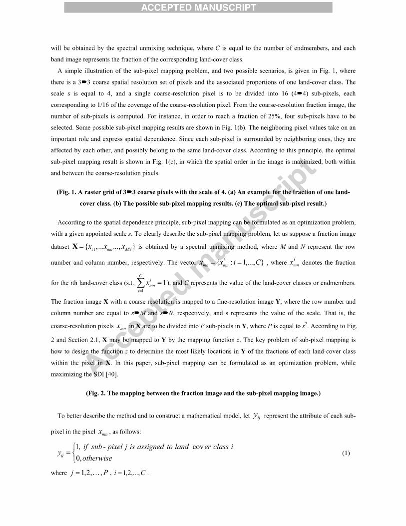
band image represents the fraction of the corresponding land-cover class.
A simple illustration of the sub-pixel mapping problem, and two possible scenarios, is given in Fig. 1, where
there is a 3�3 coarse spatial resolution set of pixels and the associated proportions of one land-cover class. The
scale s is equal to 4, and a single coarse-resolution pixel is to be divided into 16 (4�4) sub-pixels, each
corresponding to 1/16 of the coverage of the coarse-resolution pixel. From the coarse-resolution fraction image, the
number of sub-pixels is computed. For instance, in order to reach a fraction of 25%, four sub-pixels have to be
selected. Some possible sub-pixel mapping results are shown in Fig. 1(b). The neighboring pixel values take on an
important role and express spatial dependence. Since each sub-pixel is surrounded by neighboring ones, they are
affected by each other, and possibly belong to the same land-cover class. According to this principle, the optimal
sub-pixel mapping result is shown in Fig. 1(c), in which the spatial order in the image is maximized, both within
and between the coarse-resolution pixels.
(Fig. 1. A raster grid of 3�3 coarse pixels with the scale of 4. (a) An example for the fraction of one land-
cover class. (b) The possible sub-pixel mapping results. (c) The optimal sub-pixel result.)
According to the spatial dependence principle, sub-pixel mapping can be formulated as an optimization problem,
with a given appointed scale s. To clearly describe the sub-pixel mapping problem, let us suppose a fraction image
dataset 11{ ,... ..., }mn MNx x x�X is obtained by a spectral unmixing method, where M and N represent the row
number and column number, respectively. The vector },...,1:{ Cixx imnmn �� , where i
mnx denotes the fraction
for the ith land-cover class (s.t. ��
�C
i
imnx
11), and C represents the value of the land-cover classes or endmembers.
The fraction image X with a coarse resolution is mapped to a fine-resolution image Y, where the row number and
column number are equal to s�M and s�N, respectively, and s represents the value of the scale. That is, the
coarse-resolution pixels mnx in X are to be divided into P sub-pixels in Y, where P is equal to s2. According to Fig.
2 and Section 2.1, X may be mapped to Y by the mapping function z. The key problem of sub-pixel mapping is
how to design the function z to determine the most likely locations in Y of the fractions of each land-cover class
within the pixel in X. In this paper, sub-pixel mapping can be formulated as an optimization problem, while
maximizing the SDI [40].
(Fig. 2. The mapping between the fraction image and the sub-pixel mapping image.)
To better describe the method and to construct a mathematical model, let ijy represent the attribute of each sub-
pixel in the pixel mnx , as follows:
1, - cov 0,ij
if sub pixel j is assigned to land er class iy
otherwise�
� ��
(1)
where Pj ,,2,1 �� , Ci ,...,2,1� .

The spatial dependence mathematical model z is computed by the following equation [12]:
1 1
C P
ij iji j
Maximize z y I� �
� ��
s.t. ��
�C
iijy
11
1
Ps
ij ij
y N�
��
(2)
where siN is the number of sub-pixels that have to be assigned to land-cover class i, and ijI represents the SDI of
the jth sub-pixels with the ith classes.
The method uses the fraction values of neighboring pixels to find the sub-pixel location of the fractions inside
the pixel under consideration. The neighboring pixels are considered to have an influence, attracting the sub-pixels
of the same class in the neighboring pixels. So, the spatial dependence index ijI can be calculated as follows:
1
nN
ij k kk
I w f�
�� (3)
where kw is the weight of each neighboring pixel, Nn is the number of neighboring pixels, and kf is the fraction
of the kth neighboring pixel around mnx for the ith land-cover class. Thus, the sub-pixel mapping problem of P
sub-pixels with C land-cover classes can be suitably formulated as an optimization problem to find the global
maximum of the criterion function z (see also equation (2)).
2.2 Artificial immune systems and the clonal selection algorithm
Artificial immune systems (AIS), inspired by human immune systems, are a relatively new paradigm in the
domain of computational intelligence (CI). They apply several features of the human immune system, such as
recognition, detection, and elimination of foreign threats and non-self entities, while having the ability to learn [41].
Similar to the human immune system’s response to non-self entities or antigens (Ag), the AIS will archive and
update a pool of candidate solutions (antibodies) to the problem. The pool of candidate solutions is associated with
the problem, with an affinity measure indicating their fitness. In the field of AIS, the antigens can be defined as the
optimal solutions, while the antibodies are the candidate solutions trying to match the antigens. In this paper, CSA
is used as the main optimization method.
CSA derived from the adaptive immune response is formulated based on the clonal selection principle. It
imitates the learning and affinity maturation processes deployed by B-cells in the human immune system. In CSA,
the initial naive antibodies’ affinities to an antigen are tested, where the antigens are the targeted optimal solutions
and the antibodies are possible solution vectors. CSA exploits the clonal selection, proliferation, and differentiation
features to design a selection method in a way to reproduce good antibodies and replace weak antibodies. In CSA,
antibodies with good affinity are selected as parents and lead to proliferation, producing multiple offspring. These
cloned individuals undergo affinity maturation to attain better affinity from genetic changes by using a

hypermutation process. Hypermutation helps antibodies in the cloned set to exploit their local area in the decision
space. Antibodies with low affinity will be eliminated and replaced by new antibodies, to ensure diversity.
Newcomers help explore unexplored areas in the search space. In addition, the immune system develops a memory
from the previous attack of antigens. This gives the body a fast immune response for the second attack from the
same or similar antigens. The above immune processes guarantee that the algorithm may converge to the optimal
solution from the locally optimal results [29]. CSA can be described in the following steps.
1) The algorithm starts with an initial set of antibody population B and an empty memory cell set Mc.
2) For each input antigen g, it is presented to the population B and its affinity determined with each element of
B.
3) The selection process then selects the n best antibodies of B to generate a new population {n}B , according to
the affinity.
4) The clonal process reproduces a population of clones PC from the population of Bn antibodies. The higher the
affinity, the higher the number of copies, and vice versa.
5) The hypermutation process mutates all these copies at a proportional rate to create the population *C . The
higher the affinity, the smaller the mutation rate.
6) The reselection process reselects the mutated antibodies from *C and updates the memory set Mc.
7) The diversity introduction process replaces d antibodies with new antibodies Nd.
8) Repeat 2) to 7) until a certain criterion is met.
Step 5 assigns a lower mutation rate for higher affinity antibodies than lower affinity antibodies. The idea is that
the antibodies close to a local optimum need only be fine-tuned, whereas antibodies from the global optimum
should move by larger steps toward an optimum or other regions of the affinity landscape. In Step 7, the lower
affinity antibodies will have a higher probability of being replaced. The selection process leads the population
toward more stimulated antigens (the objective function or the optimal solution), while the mutation and diversity
introduction processes help to maintain the diversity of the population [37]. CSA has been presented as a distinct
method, in relation to GA, in which the type of mutation and method of reproduction are both novel, as is the two-
stage evaluation-selection operation per generation [24]. As a novel optimization algorithm, CSA has been
successfully applied to several fields, including feature selection [35], classification [36], [37], and optimization
[38], [39]. Additionally, the theoretical convergence of this algorithm, and similar algorithms (e.g. the B-cell
algorithm [42]), have also been proved by Markov chain analysis [23], [34], [43], [44]. In this paper, we investigate
the ability of CSA to solve the sub-pixel mapping problem for remote sensing imagery.
3. The clonal selection sub-pixel mapping (CSSM) framework
In this paper, a sub-pixel mapping framework based on AIS, namely, the clonal selection sub-pixel mapping
(CSSM) algorithm, is proposed to perform the task of sub-pixel mapping for remote sensing imagery. In this
section, the sub-pixel mapping problem is transformed into an optimization problem, maximizing the spatial
dependence mathematical model z (equation (2)). The CSA, inspired by AIS, as a novel optimization method, is

used to solve the optimization problem. Inspired by CSA, CSSM incorporates the idea of clonal selection. The
principle of clonal selection forms the core of AIS, where the antibodies that best fit the antigens are cloned in
order to replicate good individuals. The immunological memory cell is the best antibody solution from the cloned
cell. The antigen is regarded as the optimal solution for the objective function (e.g. equation (2)). The analogy of
the antibodies of the natural immune system is the solution to the problem, i.e., the possible sub-pixel mapping
solution. The objective is for the antibodies to fit the antigen as closely as possible and, in this case, to get as close
as possible to the optimal sub-pixel mapping solution for the remote sensing imagery. To better describe the
relation between immune systems and CSSM, the mapping table is shown in Table 1.
(Table 1 Mapping between immune systems and CSSM.)
To each pixel { : 1,..., }imn mnx x i C� � ( NnMm ���� 1,1 ) in X, the CSSM algorithm consists of the
following steps. In this section, CSSM based on Gaussian mutation (G-CSSM) is taken as an example to explain
the principle of the CSSM framework. The other mutation operators (Cauchy and non-uniform mutation) are
described in detail in Section 4.
3.1 Calculating the number of sub-pixels for each land-cover class i
In the first step, the number of sub-pixels for each land-cover class i, siN , is designed according to the following
equation:
int( )s ii mnN P x� �
��
�C
i
imnx
1
1 (4)
where P is the total number of sub-pixels s2, imnx denotes the fraction for the ith land-cover class, and C is the
number of land-cover classes.
3.2 Initialization
In this initial step, a random initial antibody population B of size BN is created, where { :1 }t Bab t N� � �B .
Each antibody tab in CSSM represents a possible sub-pixel configuration of the pixel and is directly described by
an integer string consisting of integer numbers, where the length of each antibody string is equal to the number of
sub-pixels. The antibody },,,{ 21 Pt bbbab �� , where the value of each bit in the string tab represents the class
of each sub-pixel. Because the number of sub-pixels for each class siN has been calculated by the fraction images
in advance, the algorithm should satisfy the limitations of equation (2). The set of memory cell Mc is empty, and
�cM .

The initial process is as follows: for each class i, select the unselected siN sub-pixels using the following
equation, until all the sub-pixels have been assigned to the land-cover class. If a sub-pixel has been selected, it will
not be selected again.
(1, )j Irandom P� (5)
ib j � (6)
where j represents the selected location or position of the sub-pixels, P is the number of sub-pixels, C is the number
of land-cover classes, and the function Irandom(1, P) returns a random integer value with the range [1, P].
Fig. 3 shows a simple example to illustrate the initial antibody population B at the scale of 4. Let us suppose that
}75.0,25.0{�mnx , with two classes (C =2), and each antibody tab describes a possible solution.
(Fig. 3. Illustration of the initial antibody population (two classes).)
3.3 Calculation of affinity
According to the initial antibody population, the affinities of all N antibodies in the antibody population B are
calculated using the affinity function )( tabFF � , using equations (1)–(3).
1 1
( )C P
t ij iji j
F F ab z y I� �
� � � �� (7)
where the value of ijy is obtained according to the antibody string tab . For example, for the
}1,1,1,1,1,2,1,2,2,1,2,1,1,1,1,1{�tab in Fig. 3, }1,1,1,1,1,0,1,0,0,1,0,1,1,1,1,1{1 �jy and }0,0,0,0,0,1,0,1,1,0,1,0,0,0,0,0{2 �jy ,
and the affinity of tab is:
1,1 1,2 1,3 1,4 1,5 1,7 1,10 1,12 1,13
1,14 1,15 1,16 2,6 2,8 2,9 2,11
( ) ( ) ( )
tF ab I I I I I I I I II I I I I I I
�
(8)
ijI represents the SDI of the jth sub-pixels with ith classes. Unlike equation (3), the proposed algorithms can
adaptively adjust the neighboring pixels, for boundary pixels in particular, and the number of the neighboring
pixels is changed. So, the equation (3) about the SDI is changed, using the average of the SDI, as in the following
equation:
1
nN
k kk
ijn
w fI
N���
(9)
In addition, it is worth noting that the value of the weight kw is inversely proportional to the Euclidean distance
(dis) between the sub-pixels in the fine spatial resolution sub-pixel map and the neighboring pixels in the coarse
fraction image.
3.3.1 The coordinate conversion

In this paper, the weight kw is calculated using the reciprocal of the distance by equations (10) and (11). The
shorter the distance, the greater the weight. During the process of the calculation, because each pixel is divided into
s2 sub-pixels, the sub-pixels and the pixels are located in the different scale spaces, which are in the fine spatial
resolution sub-pixel map and the coarse fraction image, respectively. We assume that the original coordinate of the
pixel is (m,n) in the coarse fraction image with an XY coordinate system, and that of the sub-pixel is (g,h) within
the pixel in the fine spatial resolution sub-pixel map with an xy coordinate system. It is necessary to project the
coordinate of the sub-pixels (g,h) and the pixels (m,n) to the same coordinate systems, X’Y’ coordinate system, by
equations (12) and (13). The new coordinates of the pixel (m, n) and the sub-pixel (g, h) are converted to (m’, n’)
and (g’, h’), according to the following equations, in which s represents the sub-pixel mapping scale.
dw /1� (10)
2''2'' )()( hngmd ��� (11)
' '( , ) ( , )m n s m s n� (12)
' '( , ) ( , )g h s g s n� (13)
(Fig. 4. The coordinate conversion and the distance calculation between the pixels and sub-pixels.)
The process of the coordinate conversion is illustrated in Fig. 4 by a simple example with the scale of 4. The
pixel is (1.5, 0.5) in the XY coordinate system, and the sub-pixel is (0.5, 1.5) in the xy coordinate system, and they
are converted to (6, 2) and (4.5, 5.5) in the new coordinate system, X’Y’, using (11) and (12), respectively.
According to equations (10) and (11), the weight of the neighboring pixel in the upper left corner of the sub-pixels
is equal to 0.263.
3.3.2 Adaptively selecting neighboring pixels
Some previous methods, such as BPSM, do not undertake sub-pixel mapping for the boundary pixels, and some
sub-pixel information in the sub-pixel mapping results is lost. To avoid this problem, the proposed method
adaptively selects the valid neighboring pixels, as in the following equation:
, ,[ ] { | ( ) [(max(1, 1) min( 1, )) (max(1, 1) min( 1, )]
[(1 ) (1 )]}m n i jN p p i m j n m i m M n j n N
m M n N� � � � � � � � � � � �
� � � � � � (14)
where M and N represent the row number and column number, respectively.
3.4 Selection
From the antibody population B, the ‘n’ highest affinity antibodies are selected to compose a new set {n}B of
high-affinity antibodies, and the highest affinity antibody cell is found to become the memory cell mc. In this step,
to better evolve the algorithm by extending the search space, the algorithm often assigns Bn N� , that is,
antibodies tab (t = 1,…, BN ) from the antibody population B will be selected for the following affinity
maturation steps, including cloning and mutation.

3.5 Cloning
After receiving antibody individuals closer to the solution, the next generation should mainly be derived from
the better-fitting individuals. Thus, the n selected abs are cloned based on their antigenic affinities, generating the
clone set PC. Each antibody tab asexually produces cn clones, according to the following equation:
( )c Bn round N�� (15)
where � is a multiplication factor defined by the user, and nc is the number of clones produced for each antibody
in the population. The function round(·) denotes the rounding operation to the nearest integer. To guarantee that
each antibody has a clonal antibody to be used in the following process, at the least, nc is set to 1 if nc is less than 1.
By the above clonal process, each antibody tab has its antibody set 1 2{ , , , }cnt t tab ab ab�tC � , where
ltab , 1,2, , cl n� � . Therefore, the cloned antibody population of the whole antibody population B,
{ : 1, , }Bt N� �C tP C � , can be obtained .
3.6 Mutation
The mutation operator provides a mechanism for solutions to escape from local regions, and to create more
diversity. Where clonal selection differs from other genetic and evolutionary computation (GEC) methods is in its
mechanism for adjusting the mutation. Unlike evolutionary strategies and mutation based on GAs, which control
the degree of mutation or the degree of mutation change by constants, the clonal selection’s degree of mutation is
functionally related to the fitness of the solution – solutions with a small deviation from the optimum have small
degrees of mutation [24].
Each clone ltab in the clone set tC has the opportunity to produce mutated offspring *
tC . The higher the
affinity, the lower the mutation rate. The rate of mutation mp plays an important role in the mutation process. If
the mutation rate is minimal, there will be too many similar individuals. On the other hand, having a high mutation
rate directs the search toward random search and increases the possibility of disrupting the structure of antibodies
that may carry good solutions. Generally, previous research papers have shown that using a fixed mp throughout
the whole evolution process is not optimal and efficient [41]. To improve the intelligence of CSSM, the mutation
rate of each cloned antibody, pm, is adaptively determined according to its affinity, as follows:
'exp( ( ))m tp F ab�� � 1, , Bt N� � (16)
where � is a decay constant defined by the user (the default value is set to 2), and the affinity of the antibody is
normalized into the range [0,1]
))(min())(max(
))(min()()('tt
ttt abFabF
abFabFabF�
�� 1, , Bt N� � (17)
Based on the mutation rate mp , the members of set *tC are produced as follows.
lt
lt abab �* 1�l (18)
)(* lt
lt abmutateab � 1, , Bt N� � , 2, , cl n� � (19)
where *ltab is the hypermutated antibody of l
tab . In order to maintain the best antibody for each clone during
evolution, the algorithm keeps one original parent antibody for each clone unmutated during the maturation phase,
i.e., 1*1tt abab � .
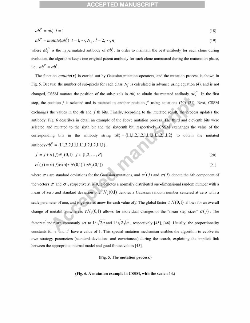
The function )(�mutate is carried out by Gaussian mutation operators, and the mutation process is shown in
Fig. 5. Because the number of sub-pixels for each class siN is calculated in advance using equation (4), and is not
changed, CSSM mutates the position of the sub-pixels in ltab to obtain the mutated antibody *l
tab . In the first
step, the position j is selected and is mutated to another position j� using equations (20)–(21). Next, CSSM
exchanges the values in the jth and 'j th bits. Finally, according to the mutated result, the process updates the
antibody. Fig. 6 describes in detail an example of the above mutation process. The third and eleventh bits were
selected and mutated to the sixth bit and the sixteenth bit, respectively. CSSM exchanges the value of the
corresponding bits in the antibody string }2,1,1,2,1,1,1,1,1,1,2,1,2,1,1,1{�ltab to obtain the mutated
antibody }1,1,1,2,1,2,1,1,1,1,1,1,2,2,1,1{* �ltab .
' ( ) (0,1)jj j j N�� },,2,1{ Pj �� (20)
))1,0()1,0(exp()()( ''jNNjj ���� � (21)
where � s are standard deviations for the Gaussian mutations, and )(' j� and )( j� denote the j-th component of
the vectors � and '� , respectively. N(0,1) denotes a normally distributed one-dimensional random number with a
mean of zero and standard deviation one. )1,0(jN denotes a Gaussian random number centered at zero with a
scale parameter of one, and is generated anew for each value of j. The global factor ' (0,1)N� allows for an overall
change of mutability, whereas (0,1)jN� allows for individual changes of the “mean step sizes” ( )j� . The
factors '� and� are commonly set to n2/1 and n2/1 , respectively [45], [46]. Usually, the proportionality
constants for � and � � have a value of 1. This special mutation mechanism enables the algorithm to evolve its
own strategy parameters (standard deviations and covariances) during the search, exploiting the implicit link
between the appropriate internal model and good fitness values [45].
(Fig. 5. The mutation process.)
(Fig. 6. A mutation example in CSSM, with the scale of 4.)

By the mutation process, the mutated antibody population 1* 2* *{ , , , }nct t tab ab ab�*
tC � for the antibody ltab is
obtained. The cloning and mutation processes are repeated until all the antibodies tab (t = NB) have been
maturated to build up the total matured antibody population *{ : 1, , }t BC t N� �*C � .
3.7 Recalculation of affinity and reselection
Evaluate the affinity for each antibody in the matured antibody population *C to obtain )( *ltabF , 1, , Bt N� � ,
2, , cl n� � . From the mature clone set C*, reselect the n abs with the highest affinity to replace the n abs with the
lowest affinity in B. Select the highest affinity ab in C* to be a candidate memory cell candidatemc .
3.8 Update of the memory cell
Compare the affinity of the candidate memory cell )( candidatemcF with the affinity of the original memory
cell )(mcF . If )( candidatemcF is higher than )(mcF , ( )()( mcFmcF candidate � ), the candidate memory cell
candidatemc will become the new memory cell, that is, candidatemcmc � .
3.9 Displacement
In order to avoid running into a locally optimal solution and to keep the diversity of the antibody population, d
new antibodies are produced by an initial process to replace the d lowest affinity abs from B. This step can increase
the diversity of the antibody population.
3.10 Stopping condition
The stopping condition is different in different applications. One option is to set a fixed number of iterations as
the stopping condition. Another option is to set a fixed threshold, e.g., the change threshold of the memory cell
between two consecutive iterations. When the maximum generation number is not met, or the change values of the
memory cell between two consecutive iterations is less than the change threshold, go to Step 3.3. Otherwise, output
the memory cell as the sub-pixels of the pixel mnx . The above process is repeated from Step 3.1 until the sub-
pixels of all the pixels are located.
Finally, the proposed algorithm outputs the sub-pixel mapping image. The flowchart for the CSSM framework is
shown in Fig. 7.
(Fig. 7. The flowchart for the CSSM framework.)
In the proposed CSSM framework, the determination of the sub-pixel spatial distribution relies upon the
information of the area ratio of the endmember components. Compared with some other sub-pixel mapping

algorithms, e.g., neural networks, which need training data, CSSM can directly obtain the optimal sub-pixel
mapping result by the artificial immune operators, without training data.
4. Extended clonal selection sub-pixel mapping algorithms
The mutation operator is the key search operator that generates new solutions from the current ones in the CSSM
framework. In G-CSSM, each antibody is mutated with the mutation rate via Gaussian mutation, which produces
new properties of the mutated antibodies. One possible problem with Gaussian mutation in solving some of the
multimodal optimization problems is its slow convergence to a good near-optimum [46]–[48]. In this section, to
avoid the problem, two new mutation operators (Cauchy mutation and non-uniform mutation) are developed to
propose two novel sub-pixel mapping algorithms.
4.1 Clonal selection sub-pixel mapping algorithm based on Cauchy mutation (C-CSSM)
Cauchy mutation is an efficient search operator for a large class of multimodal function optimization problems,
and it has the ability to escape local minima [46]. Cauchy mutation can increase the probability of finding a near-
optimum by long jumps when the distance between the current search point and the optimum is large, but it will
decrease the probability when such distances are small [46]. Because Cauchy mutation has the long jumps, it is
more suitable for the processing of very high volume data, e.g., remote sensing imagery.
The general formula for the probability density function of the Cauchy distribution is defined by:
2
1( ) ,�(1 (( ) / ) )
f x xs x t s
� �� � � � �
(22)
where t is the location parameter, and s is the scale parameter [49]. The case where t=0 and s=1 is called the
standard Cauchy distribution. The equation for the standard Cauchy distribution reduces to:
2
1( )�(1 )
f xx
�
(23)
Since the general form of the probability function can be expressed in terms of the standard distribution, all
subsequent formulae in this paper are given for the standard form of the function. The corresponding distribution
function is:
1 1( ) arctan( )2 �
F x x� (24)
The shape of ( )f x resembles that of the Gaussian density function but approaches the axis so slowly that an
expectation does not exist [46]. As a result, the variance of the Cauchy distribution is infinite. Fig. 8 shows the
probability density function of the Cauchy distribution.
(Fig. 8. Cauchy and Gaussian density functions.)
The C-CSSM studied in this paper is exactly the same as the CSSM described in Section 3, except for equation
(20), which is replaced by the following equation [46] to mutate the clonal antibodies:

' ( ) (0,1)jj j j C�� (25)
where )1,0(jC denotes a Cauchy random number with the standard Cauchy distribution, and is generated anew for
each value of j.
To better show the ability of Cauchy mutation, the Gaussian functions are also shown and compared with
Cauchy mutation by plotting them at the same scale in Fig. 8. It is clear from Fig. 8 that Cauchy mutation is more
likely to generate an offspring further away from its parent than Gaussian mutation, due to its long flat tails. It is
expected to have a higher probability of escaping from a local optimum or moving away from a plateau, especially
when the “basin of attraction” of the local optimum or the plateau is large relative to the mean step size. On the
other hand, the smaller hill around the center in Fig. 8 indicates that Cauchy mutation spends less time in
exploiting the local neighborhood and, thus, has a weaker fine-tuning ability than Gaussian mutation in small- to
mid-range regions. The results of the experiments have shown that the Cauchy mutation can be successfully
applied to make evolutionary programming faster [46]. This fact encourages us to conclude that C-CSSM has a
much better performance than CSSM.
4.2 The clonal selection sub-pixel mapping algorithm based on non-uniform mutation (N-CSSM)
In addition to Cauchy mutation, a new mutation operator, non-uniform mutation, is used to propose a clonal
selection sub-pixel mapping algorithm based on non-uniform mutation (N-CSSM). A non-uniform mutation
operator is one of the operators responsible for fine-tuning capabilities and was originally proposed to reduce the
disadvantage of random mutation in evolutionary algorithms [50]. Compared with G-CSSM, the proposed N-
CSSM algorithm has a similar sub-pixel mapping process, except for the mutation operator, as the Gaussian
mutation operator is replaced by the non-uniform mutation operator, using the following equation:
' ( , ) 0,( , ) 1
j t UB j if a random isj
j t j LB if a random is��
� ��� � �� ��
(26)
where LB and UB are the lower and upper bounds of the variable j, respectively. In N-CSSM, LB is equal to 1 and
UB is equal to the number of the sub-pixels s2.
The function ),( yt� returns a value in the range [0, y], such that ),( yt� approaches zero as t increases. This
property allows this operator to search the space uniformly at early stages (when t is small), and very locally at
later stages [51]. ),( yt� is calculated using the following equation:
���
�
�
!
"����
���
!" �
b
Tt
ryyt1
1),( (27)
where r is a uniform random number from [0,1], T is the maximal generation number, and b is a system parameter
determining the degree of non-uniformity.
In the initial generations, N-CSSM tends to search the solution space uniformly, and in the later generations it
tends to search the space locally, i.e., closer to its descendants, using the non-uniform mutation operator.
4.3 Complexity analysis

Although there are three proposed algorithms, their sub-pixel mapping frameworks are all based on CSA. This
section presents a general evaluation of the complexity of the CSSM algorithms, taking into account the
computation cost per generation for the sub-pixel mapping of each pixel. The computation time of the proposed
algorithms can be measured by counting the maximum number of instructions executed, which is proportional to
the maximum number of times each loop is executed. Regardless of the affinity function, the same parameters are
used to characterize the computations performed [32], including the dimension of the antibody Ab, P, the total
number of clones, cn , the number of Ag’s to be sub-pixel mapped, M N , and the number of selected Ab’s for
clone n. For the sub-pixel mapping problem, P is equal to s2.The proposed algorithms have three main processing
steps:
1) determining the affinity of the Ab’s (see also Section 3.3)
2) selecting and reselecting the n highest affinity Ab’s (see also Sections 3.4 and 3.7)
3) hypermutating the population C (see also Section 3.6)
The usual way of selecting n individuals from a population is by sorting the affinity (fitness) vector f and then
extracting the n first elements of the sorted vector. This can be performed in ( )O n time. For our proposed
algorithms, the computation time required in Sections 3.4 and 3.7, the selection and reselection phases, is ( )BO N
and ( )cO n in the worst cases, where Bn N� and cn n� , respectively. Mutating the cn clones demands a
computation time of the order ( )cO n P . By summing up the computation time required for each of these steps, it is
possible to determine the total computation time of the algorithm. In the sub-pixel mapping case, these steps have
to be performed for each of M N Ag’s (pixels). Therefore, the computation time of the whole process comes
preceded by a multiplication factor of M N . That is, the computational complexity of the algorithms is
( ( ))B cO M N N n P .
5. Experiments and analysis
Three experiments were conducted to evaluate the performance, efficiency, and functionality of the proposed
algorithms (G-CSSM, C-CSSM, N-CSSM), using synthetic images and one real image. The methods of data
preparation and accuracy assessment are described in detail in Section 5.1.1. Consistent comparisons were carried
out between G-CSSM, N-CSSM, C-CSSM and the following sub-pixel mapping algorithms: direct neighboring
sub-pixel mapping (DNSM) [19], the sub-pixel mapping algorithm based on spatial attraction models (SASM) [20],
the BP neural network sub-pixel mapping algorithm (BPSM) [10], and the sub-pixel mapping algorithm based on a
genetic algorithm (GASM) [13]. The configuration for BPSM (using one hidden layer) was as follows: The number
of hidden layers, the learning rate, and momentum rate were 1, 0.25, and 0.9, respectively. In the experiments, 50
training samples for each class were randomly selected as the training samples for BPSM. The crossover rate and
mutation rate for GASM were set to 0.5 and 0.05, respectively. The antibody population size BN , the
multiplication factor � , and the number of displaced antibodies d were 100, 0.02, and 10, respectively. In

addition, all the algorithms only considered the surrounding neighboring pixels [10], that is, the eight neighboring
pixels.
5.1 Methods of data preparation and accuracy assessment
5.1.1 Data preparation
In the experiments, the sub-pixel mapping algorithms should ideally be applied on fraction images of a certain
spatial resolution and compared with the results of a hard classification on a finer resolution. However, in this
process, there are some extra errors inherent in real imagery, caused by the sensor point spread function,
atmospheric and geometric effects, and classification or spectral unmixing errors [13]. To avoid any uncertainty,
synthetic images were used in the first two experiments. Firstly, the hard classification image by a remote sensing
classifier (e.g. support vector machine (SVM) [52]) is regarded as the output reference image. Then, the input
fraction images with a coarser scale are derived by degrading the hard classification data using an averaging filter.
Synthetic imagery has the advantage of lacking co-registration errors between the lower- and the higher-resolution
images. Previously, other researchers have described more complex methods for spatially degrading images, based
upon the sensor’s point spread function [12], [53]. For the purpose of evaluating the performance of the sub-pixel
mapping algorithm, however, this paper utilizes synthetic images obtained by the above process and does not
model the effect of the point spread function, as have most other sub-pixel mapping studies [17].
The resulting sub-pixel mapping classification does not contain any uncertainty as it originates from
degradation, instead of a classification or spectral unmixing process. Consequently, the sub-pixel mapping solely
reflects the performance of the proposed methodology [6]. Sub-pixel mapping results can then be compared to the
original hard classification (reference image), as well as the hardened version of the fraction images (hard
classification) [19]. For simulated images, different resolution levels require sub-pixel algorithms implemented
with different scale factors. In this research, the scale factor was set to 4. The sensitivity in relation to the value of
scale will be discussed in detail in Section 6.
A synthetic process has been the common method of obtaining the experimental images in the previous research
work on sub-pixel mapping. Although synthetic images may avoid the reflection of other errors (e.g. co-
registration error), our research work is aimed at applying the sub-pixel mapping technique to real imagery.
Therefore, in the third experiment, we utilized real images with different scales (TM and IKONOS images of
Shenzhen city, China), from the same research area, to test the performance of the sub-pixel mapping algorithms.
5.1.2 Accuracy assessment
The accuracy was measured by comparing the output of the sub-pixel mapping to the reference image, as
mentioned before. As with the classification, the overall accuracy (OA) in terms of the percentage of correctly
mapped sub-pixels, and the Kappa coefficient [54] based on the confusion matrix were utilized to evaluate the
accuracy of the different sub-pixel mapping algorithms’ results. Columns in a confusion matrix typically represent
the reference data, and rows represent the sub-pixel mapping data. The OA is simply the sum of the sub-pixels

mapped correctly (i.e. the diagonal elements) divided by the total number of samples in the comparison. The Kappa
coefficient can be defined in terms of the confusion matrix, as follows.
�
� �
�
� �
�
�� r
kkk
r
k
r
kkkkk
xxL
xxxLKappa
1
2
1 1
)(
)( (28)
where r is the number of rows in the matrix, kkx is the number of observations in row i and column j , kx and
kx are the marginal totals for row i and column j , respectively, and L is the total number of observations.
OA and Kappa consider all the pixels of the image, including the pure pixels as parents in the finer resolution.
These sub-pixels all belong to the pure pixels and will only raise the value of OA and Kappa, without providing
information about the algorithm’s prediction abilities [13]. To improve the reliability, the adjusted OA (OA*) and
Kappa coefficient (Kappa*) were also considered to evaluate the sub-pixel mapping algorithms, where OA*and
Kappa* are calculated only for mixed pixels, that is, they ignore the sub-pixels that have a pure pixel as a parent. In
general, OA*and Kappa* provide an indication of the ability of the algorithm to produce an accurate sub-pixel
mapping, whereas OA and Kappa evaluate the result of the whole image mapping. In addition, the computation
expense was another factor utilized to evaluate the algorithms.
The experimental process of the sub-pixel mapping algorithms is shown in Fig. 9.
(Fig. 9. The experimental process of the sub-pixel mapping algorithms.)
5.2 Experiment 1: synthetic images – artificial image
The artificial images were images created by the authors to aid in the design and development of the proposed
algorithms, as shown in Fig. 9. Their use was determined by their size, resulting in a considerable reduction in
computation time. Visual checking of the algorithm’s performance is easy with these images as they represent
simple geometric figures [6]. In this experiment, a simple three-class (C1, C2, and C3) image was chosen to
illustrate the functionality of the technique, as shown in Fig. 10(a). The results were evaluated using a real hard-
classified image by SVM, as shown in Fig. 10(b), and the test samples for C1, C2, and C3 were 281356, 545556,
and 79392, respectively. In addition, to calculate the OA* and the Kappa*, the test samples for mixed pixels of C1,
C2, and C3 were 6060, 9652, and 4672, respectively. Fig. 10(c) illustrates the degraded fraction image with a scale
of 4 from a hard classification image. The sub-pixel mapping results using the DNSM, SASM, BPSM, G-CSSM,
C-CSSM, and N-CSSM algorithms are shown in Fig. 10(d)–(i). For a clear comparison of the CSSM algorithms
with the other algorithms, a small area (S1) of the C1 class is zoomed and is shown in Fig. 10(k).
A visual comparison of the results of the seven sub-pixel mapping algorithms in Fig. 10 suggests varying degrees of
accuracy of sub-pixel mapping, but they do exhibit a similar overall sub-pixel mapping appearance. However, for mixed
pixels, it can be seen that the result of the BPSM algorithm is not satisfactory; for example, the sub-pixel mapping results
of BPSM look blurred and exhibit sawtooth patterns in the C1 class. In addition, BPSM does not obtain the boundary
sub-pixel mapping results, which are represented by black pixels. DNSM also does not give satisfactory results. GASM,
SASM, C-CSSM, and G-CSSM have better visual results than BPSM and DNSM, but there are blurry scenes in the C1

class for GASM, SASM, and C-CSSM. The proposed N-CSSM suffers less from this side effect and makes the border of
the classification image smooth. As a result, the sub-pixel mapping result obtained by N-CSSM gave a better visual
result for the artificial image experiment.
(Fig. 10. The sub-pixel mapping results in experiment 1 (scale = 4). (a) Original artificial image (960�960).
(b) Original hard classification result (960�960). (c) The fraction images (240�240). (d) DNSM. (e) SASM.
(f) BPSM. (g) GASM. (h) G-CSSM. (i) C-CSSM. (j) N-CSSM. (k) Zooms for (b) and (d)–(j).)
The original hard classification result is considered as the reference image. For a more detailed verification of
the results, the OA, Kappa coefficient, OA*, Kappa*, and computation time were used to evaluate the performance
of the sub-pixel mapping algorithms. To evaluate the statistical reliability of the stochastic sub-pixel mapping
algorithms, GASM and the CSSM algorithms were run 10 times and their average accuracies were considered.
Table 2 lists the results of comparisons between the original hard classification image and the sub-pixel mapping
images obtained by the seven algorithms: DNSM, SASM, BPSM, GASM, G-CSSM, C-CSSM, and N-CSSM.
(Table 2 A comparison of the seven sub-pixel mapping algorithms’ performance in experiment 1.)
As shown in Table 2, the N-CSSM algorithm produces better sub-pixel mapping results than the other six
algorithms, i.e., the best OA and OA*, 99.99% and 99.49%. N-CSSM improves the Kappa and Kappa* from
0.9871 to 0.9998, and 0.5166 to 0.9920, improvements of 0.0127 and 0.4754, respectively. It is worth noting that
the difference using OA* is higher than using OA. This is due to the existence of the mixed pixels and, as a result,
OA* is more suitable for evaluating the performances of the sub-pixel mapping algorithms. In this experiment,
BPSM cannot correctly map many pixels and has a low degree of accuracy. One reason for this could be that
BPSM is sensitive to the training samples; we randomly selected 50 training samples in this experiment. If more
good training samples are used, it could lead to better results. Because DNSM does not consider the distance
between the central pixel and the neighboring pixels, it only obtains a low sub-pixel mapping accuracy. SASM
improves DNSM by considering different distances as the weight, and it obtains a satisfactory sub-pixel mapping
result for the artificial image. Regarding computation time, BPNN needs 15.218s, while DNSM is most efficient,
taking only 1.063s. Unlike SASM, GASM and the three CSSMs (G-CSSM, C-CSSM, N-CSSM) transform the sub-
pixel mapping problem into an optimization problem of the SDI and use a GA and CSAs to solve the problem,
respectively. In this experiment, although the sub-pixel mapping result provided by GA is better than DNSM and
BPSM, it does not outperform those provided by SASM and the CSSMs. One reason for this could be that the
simple GA was used in the experiment, which seems to present a tendency toward premature convergence. In
addition, as with GA, CSA is a heuristic algorithm. However, their underlying mechanisms and methods of
evolutionary search differ significantly in terms of inspiration, vocabulary, and fundamentals. CSA utilizes the
shape-space formalism inspired from immunological terminology to describe antigen-antibody interactions and
cellular evolution in immune systems, while GA uses the genetic evolution principle inspired from Darwinian
evolution theory [35], [55]. So, the sub-pixel mapping algorithm based on GA (GASM) performs the process of
optimization through genetic operators, including reproduction, crossover, and mutation, while the sub-pixel

mapping algorithm based on CSA (CSSM) performs its search through the immune operators, including selection,
mutation, memory, and displacement. GASM tends to polarize the whole population of individuals toward the best
one, while CSSM maintains a diverse set of locally optimal solutions, using the memory cell inherited from the
memory property of human immune systems [32] to obtain better sub-pixel mapping results. Compared with
GASM with 95.51% and 255.341 s, N-CSSM has better sub-pixel mapping results of 99.49%, and a reduced
computation time of 108.654s.
The three CSSMs inspired by the clonal selection theory are self-adaptive methods that can adjust themselves to
the data, without any explicit specification of functional or distributional form for the underlying mode. In the
proposed algorithms, the clonal process can draw the evolutionary process closer to the best sub-pixel mapping
result, and the mutation step generates random changes of antibodies and helps the proposed algorithm to avoid
locally optimal values. Comparing the three CSSMs with SASM, G-CSSM has a similar sub-pixel mapping result
to SASM. C-CSSM using the Cauchy mutation operator does not obtain better results than SASM, although it is
expected to have a higher probability of escaping from a local optimum. One reason for this may be that the
Cauchy mutation operator is not suitable for this image, in which “long jumps” are detrimental if the current point
is already very close to the global optimal sub-pixel mapping result. N-CSSM using non-uniform mutation
operators obtains the best sub-pixel mapping results because the non-uniform mutation operator is not sensitive to
the search space size [51], and in the later generations it may search the space locally to improve the probability of
finding the optimal results. These are the reasons that N-CSSM is the best sub-pixel mapping algorithm in this
experiment.
5.3 Experiment 2: synthetic images – remote sensing images
To evaluate the performance of these sub-pixel mapping algorithms in solving a real complex problem, we tested
the sub-pixel mapping algorithm proposed in experiment 2 using two 30 m resolution multispectral Landsat TM
images and two hyperspectral remote sensing images, the Washington DC HYDICE image and the Indian Pine
AVIRIS image. The synthetic remote sensing images were obtained by degrading the hard classification data using
an averaging filter. These images lack co-registration errors between the lower- and higher-resolution images [6].
The aforementioned procedures used in the previous experiments were also utilized in the experiments on the
synthetic TM and hyperspectral images.
One of the TM images (1024×1024 pixels), as shown in Fig. 11(a), was acquired in the Namco Lake area, Tibet,
P.R. China, on June 13, 2001. This study area is a representative plateau area in the famous Qinghai-Tibetan
Plateau, and includes four classes: water, vegetation, snow, and soil. As shown in Fig. 11(a), because the season
was the summer, most of the snow had melted. Fig. 11(b) illustrates the original hard classification image as the
reference image, and the test samples for the water, vegetation, snow, and soil classes were 88628, 197996, 10046,
and 751906, respectively. In addition, to calculate the OA* and the Kappa*, the test samples for mixed pixels of
the water, vegetation, snow, and soil classes were 4564, 97500, 3134, and 122162, respectively. The fraction
images shown in Fig. 11(c) were obtained by upscaling the classification image. Fig. 11(d)–(j) illustrates the sub-
pixel mapping results using the DNSM, SASM, BPSM, GASM, G-CSSM, C-CSSM, and N-CSSM algorithms,

respectively. To ensure clarity when comparing the CSSMs with the other algorithms, the small images of the S1
area are zoomed and are shown in Fig. 11(k).
(Fig. 11. The sub-pixel mapping results for the Namco TM image in experiment 2 (scale = 4). (a) Namco TM
image RGB (4,3,2) (1024�1024). (b) Original hard classification result (1024�1024). (c) The fraction images
(256�256). (d) DNSM. (e) SASM. (f) BPSM. (g) GASM. (h) G-CSSM. (i) C-CSSM. (j) N-CSSM. (k) Zooms
for (b) and (d)–(j).)
The other TM image (400×400 pixels), as shown in Fig. 12(a), was acquired in the Three Gorges area, Hubei
Province, P.R. China, on September 1, 1999. The original TM image was classified by the SVM classification
method to obtain the reference image shown in Fig. 12(b). This study area is a representative mountainous region,
which was expected to fall into four classes: Yangtze River, lake, impervious layer (buildings, roads, etc.), and
vegetation. The test samples for the Yangtze River, lake, impervious layer, and vegetation classes were 16996,
10479, 46641, and 85884, respectively. In addition, to calculate the OA* and the Kappa*, the test samples for
mixed pixels of the Yangtze River, lake, impervious layer, and vegetation classes were 3012, 8047, 20577, and
28188, respectively. The fraction images of the four classes are shown in Fig. 12(c). The sub-pixel mapping results
obtained by DNSM, SASM, BPSM, GASM, G-CSSM, C-CSSM, and N-CSSM are illustrated in Fig. 12(d)–(j).
The small images of the S1 area are zoomed and are shown in Fig. 12(k) to assist with the evaluation of the sub-
pixel mapping algorithms from the visual results.
(Fig. 12. The sub-pixel mapping results for the Three Gorges TM image in experiment 2 (scale = 4). (a)
Three Gorges TM image RGB (4,3,2) (400�400). (b) Original hard classification result (400�400). (c) The
fraction images (100�100). (d) DNSM. (e) SASM. (f) BPSM. (g) GASM. (h) G-CSSM. (i) C-CSSM. (j) N-
CSSM. (k) Zooms for (b) and (d)–(j).)
To evaluate the performance of the proposed algorithms for more complex images, two hyperspectral images
with more land-cover classes were also used. The third synthetic remote sensing image (Washington DC dataset)
was a Hyperspectral Digital Imagery Collection Experiment (HYDICE) airborne hyperspectral image (240×240)
acquired over Washington DC. This study area is a representative urban region, which was expected to fall into six
classes: roof, road, trail, grass, shadow, and tree [56]. The test samples for the different classes were 16880, 13107,
2964, 10169, 4578, and 9902, respectively. In addition, to calculate the OA* and the Kappa*, the test samples for
mixed pixels were 11824, 11571, 2868, 6825, 4210, and 8958, respectively. The fraction images of the six classes
are shown in Fig. 13(c). The sub-pixel mapping results obtained by DNSM, SASM, BPSM, GASM, G-CSSM, C-
CSSM, and N-CSSM are illustrated in Fig. 13(d)–(j). The small images are zoomed and are shown in Fig. 13(k) to
assist with the evaluation of the sub-pixel mapping algorithms from the visual results.
(Fig. 13. The sub-pixel mapping results for the Washington DC HYDICE image in experiment 2 (scale = 4).
(a) Washington DC HYDICE image RGB (67,27,17) (240�240). (b) Original hard classification result
(240�240). (c) The fraction images (60�60). (d) DNSM. (e) SASM. (f) BPSM. (g) GASM. (h) G-CSSM. (i) C-
CSSM. (j) N-CSSM. (k) Zooms for (b) and (d)–(j).)

The other synthetic hyperspectral remote sensing original image was acquired by the Airborne Visible/Infrared
Imaging Spectrometer (AVIRIS) in June 1992. The image data (136�136 pixels) shown in Fig. 14(a) represents
the representative agricultural area of Indian Pine in the northern part of Indiana. The ten most representative land-
cover classes are: Corn-no till (C1), Corn-min till (C2), Grass/Pasture (C3), Grass/Trees (C4), Hay-windrowed
(C5), Soybeans-no till (C6), Soybeans-min till (C7), Soybeans-clean till (C8), Woods (C9), and Bldg-Grass-Tree
drives (C10). Fig. 14(b) is the reference classification map obtained by the artificial antibody network (ABNet)
classifier [57]. The test samples for the different classes were 2409, 902, 1438, 2229, 871, 2714, 2370, 671, 3096,
and 2336, respectively. In addition, to calculate the OA* and the Kappa*, the test samples with the different classes
for mixed pixels were 2073, 870, 1262, 1957, 551, 2062, 1954, 671, 2184, and 2240. The sub-pixel mapping
results using the different algorithms are shown in Fig. 14 (d)–(k).
(Fig. 14. The sub-pixel mapping results for the Indian Pine AVIRIS image in experiment 2 (scale = 4). (a)
Indian Pine AVIRIS image RGB (57,27,17) (136�136). (b) Original hard classification result (136�136). (c)
The fraction images (34�34). (d) DNSM. (e) SASM. (f) BPSM. (g) GASM. (h) G-CSSM. (i) C-CSSM. (j) N-
CSSM. (k) Zooms for (b) and (d)–(j).)
Comparing the different sub-pixel mapping results with the reference images (Fig. 11(b), Fig. 12(b), Fig. 13(b),
Fig. 14(b)), DNSM and BPSM do not obtain satisfactory results. There are many blurry regions in the sub-pixel
mapping result obtained by DNSM, as shown in Fig. 11(d), Fig. 12(d), Fig. 13(d), and Fig.14(b). Also, BPSM does
not obtain satisfactory results as the sawtooth phenomenon can be seen on the border of the classes in the sub-pixel
mapping result obtained by BPSM, i.e., the sub-pixel mapping of the water classes in Fig. 11(f) and Fig. 11(k), the
border between the impervious layer and Yangtze River or vegetation (the road on the right is not clear) in Fig.
12(f) and Fig. 12(k), the border between the roof and shadow in Fig. 13(f) and Fig. 13(k), and the border between
the different classes in Fig. 14(f) and Fig. 14(k). SASM decreases the sawtooth effects on the border between
different classes, for example, the impervious layer and Yangtze River in Fig. 12(e) and Fig. 12(k), but there are
still some sawteeth on the border between vegetation and the impervious layer, where some impervious layer pixels
were misclassified as vegetation pixels. As shown in the zoom image for Fig. 12(g), GASM also improves the sub-
pixel mapping results on the border between the impervious layer and Yangtze River, but the sub-pixel mapping
results on the border between the impervious layer and lake are not satisfactory. In contrast, the three CSSM
algorithms give similar sub-pixel mapping results and have better visual accuracy in all the sub-pixels, especially in
the mixed border of two different classes, which makes the border of the sub-pixel mapping image smooth.
The sub-pixel mapping accuracies of the two synthetic TM and two hyperspectral remote sensing images were
measured by comparing the output of the sub-pixel mapping with the reference image, as mentioned before, in
terms of OA, Kappa, OA*, and Kappa*, and are shown in Tables 3–6. It can be seen from Tables 3, 4, 5, and 6 that
the three clonal selection sub-pixel mapping algorithms, G-CSSM, C-CSSM, and N-CSSM, produce better sub-
pixel mapping results than the other four sub-pixel mapping results, with N-CSSM giving the best results. For
example, N-CSSM has the highest value of OA and Kappa. In addition, for the mixed pixel, N-CSSM also has the
highest OA* (81.72%, 77.62%, 67.51%, 63.31%) and Kappa* (0.6539, 0.6498, 0.5942, 0.5841) for the Namco and
Three Gorges TM images, the HYDICE image, and the AVIRIS image, respectively. On the whole, the accuracies

of the algorithms for the synthetic real images are lower than for the synthetic artificial image because the synthetic
real image had a higher complexity. Due to the higher complexity, DNSM and BPSM found it difficult to obtain
satisfactory results. BPSM still lost the border sub-pixel mapping information. Tables 3–6 show SASM giving
better results than DNSM and BPSM. The results provided by GASM were not as good as those provided by
SASM for the two TM images, and GA requires the most computation time, 2629.991s, 691.128s, 551.750s, and
358.031s, for the four synthetic images, respectively.
Comparing SASM with the proposed algorithms, SASM has sub-pixel accuracies that are similar to the CSSM
algorithms for the two TM images, but the proposed algorithms, especially N-CSSM, are better than SASM for the
two complex hyperspectral images with more land-cover classes. As shown in Tables 5 and 6, N-CSSM improves
the OA* from 64.10% with SASM to 67.51% (improved by 3.41%), the Kappa* from 0.5516 to 0.5942 for the
HYDICE image with six classes, the OA* from 60.80% with SASM to 63.31% (improved by 2.51%), and the
Kappa* from 0.5565 to 0.5847 for the AVIRIS image with 10 classes. It can be seen that SASM can obtain
satisfactory sub-pixel mapping results when the images or the distribution of land-cover classes are simple;
however, for more complex images, i.e., hyperspectral images, or more land-cover classes, the accuracy of SASM
needs to be improved. One possible reason for this is that SASM is not an optimal method and cannot guarantee to
obtain the optimal sub-pixel mapping result, for which SASM directly utilizes a spatial attraction model to achieve
the SDI. The proposed CSSM algorithms can obtain the optimal solution through maximizing the criterion
function, that is, the SDI.
In the three proposed algorithms, the additional cloning process may increase the average affinity values, extend
the search space, and provide the mutation steps, with a good chance of moving closer to the optimal sub-pixel
mapping result. A mutation step is also crucial in the CSSMs. It generates random changes of the cloned antibodies
(possible solution), and this helps avoid a local optimum to obtain the optimal solution. In addition, the CSSMs
inherit the memory property of human immune systems to build a memory cell population with a diverse set of
locally optimal solutions. Based on the memory cell population, the CSSMs output the value of the memory cell
and find the optimal sub-pixel mapping. Therefore, G-CSSM, C-CSSM, and N-CSSM may be better able to find
the best sub-pixel mapping results with less computation time than GASM. Inspiringly, among the three proposed
algorithms, N-CSSM using non-uniform mutation operators exhibits a better potential than G-CSSM and C-CSSM
when they are applied to the same experiment for remote sensing sub-pixel mapping. Based on the above analysis,
we can conclude that the CSSMs are better sub-pixel mapping algorithms for the remote sensing images used in
this experiment.
(Table 3 A comparison of the different sub-pixel mapping algorithms’ performance with the Namco TM
image in experiment 2.)
(Table 4 A comparison of the different sub-pixel mapping algorithms’ performance with the Three Gorges
TM image in experiment 2.)

(Table 5 A comparison of the different sub-pixel mapping algorithms’ performance with the Washington
DC HYDICE image in experiment 2.)
(Table 6 A comparison of the different sub-pixel mapping algorithms’ performance with the Indian Pine
AVIRIS image in experiment 2.)
5.4 Experiment 3: real image
The experimental images in experiments 1 and 2 were obtained by a synthetic process, which has been the
common method of obtaining experimental images in the previous research work on sub-pixel mapping. Although
synthetic images may avoid the reflection of other errors (e.g. co-registration error), the sub-pixel mapping
methods were not directly applied to sub-pixel mapping for real imagery. In the third experiment, we used the sub-
pixel mapping methods to obtain a higher-resolution classification image from a real low-resolution remote sensing
image (a 30 m ETM image). To evaluate the result, a real high-resolution classification image based on a 4 m
IKONOS image of the same research area was used to test the performance of the sub-pixel mapping algorithms.
Although there are other errors, such as the co-registration error and spectral unmixing error, these errors are the
same for all the sub-pixel mapping methods, and relative comparisons are fair.
The low-resolution remote sensing Landsat ETM image data (98�30) used in this experiment, as shown in
Fig. 15(b), refers to the Shenzhen Special Zone of China and was acquired on December 31, 2001. This product
was georeferenced with a spatial resolution of 30 m. The high-resolution IKONOS data (784�240), as shown in
Fig. 15(a), from over the same region, was acquired on December 20, 2001. Although 11 days difference exists
between the two images, both of them were acquired in the same month and year; hence, their reflectance spectra
are assumed to be similar. The representative city study area is expected to fall into four classes: bare soil,
vegetation, water, and city. To compare the sub-pixel mapping results with the classification image of the IKONOS
image, five steps were included, as follows. First, the IKONOS image shown in Fig. 15(a) was registered with the
ETM image (Fig. 15(b)) using ground control points, with a total root mean square error (RMSE) of less than 0.03.
Second, the IKONOS image was classified into four classes (city, vegetation, bare soil, and water) using SVM with
field surveying, as shown in Fig. 15(c). In this experiment, to obtain more features from the high spatial resolution
images, textural features based on gray-level cooccurrence matrix statistical parameters [58] were added to
improve the classification results, from which four statistical parameters (entropy, homogeneity, dissimilarity, and
second moment) were selected. Recent studies have found that the typical scale of urban reflectance is between 10–
20 m [59]. Therefore, most 4�4 m IKONOS pixels are spectrally homogeneous and can be reasonably assumed to
be pure material. To guarantee the accuracy of the evaluation, this step consists of computing a map of markers
using spectral-textural classification maps from the previous step, and the following rule: for every pixel, if the
output probability of the SVM classifier is larger than a certain threshold (e.g. 0.95), the pixel is kept as a marker
with a corresponding class label [60]. The resulting map, as shown in Fig.15(c), contains the most reliably
classified pixels, in which black pixels as unreliable pixels will not be used in the following steps. The test samples
for the bare soil, vegetation, water, and city classes were 19130, 14775, 7787, and 68298, respectively. In addition,

to calculate the OA* and the Kappa*, the test samples for mixed pixels of the bare soil, vegetation, water, and city
classes were 18554, 14771, 5419, and 67786, respectively. Third, the fraction images of the ETM image were
obtained by the least squares linear spectral mixture analysis method with an abundance sum-to-one constraint [61]
by ENVI� remote sensing image processing software [62]. After spectral unmixing, to satisfy the abundance
nonnegativity constraint, the fraction images were normalized to the range [0, 1] and are shown in Fig. 15(d).
Fourth, the sub-pixel mapping results using the different methods were acquired based on the fraction image with
scale=8. Finally, the classification marker map of the IKONOS image was overlaid on the sub-pixel mapping
image to estimate the sub-pixel mapping results. Fig. 15(e)–(k) illustrates the sub-pixel mapping results using
DNSM, SASM, BPSM, GASM, G-CSSM, C-CSSM, and N-CSSM. To ensure a clear comparison of the CSSMs
with the other algorithms, the small S1 area is zoomed and is shown in Fig. 15(l).
As shown in Fig. 15, the results of DNSM and BPSM show obvious sawteeth and do not have clear structural
information for land-cover classes, i.e., roads in the city class, and vegetation. SASM gives a clearer sub-pixel
mapping result than DNSM and BPSM; for example, providing a clearer border of water. However, the spatial
connectivity of some classes in SASM (e.g. vegetation) is not good, as shown in the zoom image of Fig. 15(l).
Compared with the other algorithms, GASM gives better visual results than SASM, in spite of some salt-and-
pepper noise. There is definitely better spatial connectivity for the three proposed algorithms. In Fig. 15(i)–(k), the
vegetation, bare soil, water, and city classes have good spatial connectivity. As a result, the three proposed
algorithms achieve better visual results, as shown in Fig. 15(l). It should be noted that there are some shadow
pixels in the city area due to sunshine. Some city pixels are misclassified as water classes because these shadows
have very similar spectral information to water. These shadow pixels affect the performance of all the sub-pixel
mapping algorithms.
(Fig. 15. The sub-pixel mapping results for the Shenzhen ETM image in experiment 3 (scale = 8). (a)
Shenzhen IKONOS image (784�240). (b) Shenzhen ETM image RGB (4,3,2) (98�30). (c) Shenzhen
IKONOS classification marker image. (d) The fraction images of the ETM image (98�30). (e) DNSM. (f)
SASM. (g) BPSM. (h) GASM. (i) G-CSSM. (j) C-CSSM. (k) N-CSSM. (l) Zooms for (b) and (e)–(k).)
The sub-pixel mapping accuracies for the seven sub-pixel mapping algorithms, in comparison with the original
classification image shown in Fig. 15(c), are given in Table 7. As shown in Fig. 15 and Table 7, although the
difference in the accuracy between DNSM, BPSM, and SASM is slight, SASM provides more abundant sub-pixel
land-cover class information, according to Fig. 15(e)–(g). It is worth noting that BPSM provides a better sub-pixel
mapping result than DNSM and SASM for the difficult real remote sensing images. One possible reason for this is
that BPSM does not obtain the boundary information (black pixels), due to the boundary pixels lacking
neighboring pixels, and during the process of the accuracy calculation for BPSM, the lost boundary pixels are not
used and therefore improve the accuracy. In addition, GASM also obtains better results than DNSM, SASM, and
BPSM using the optimization process maximizing the SDI [13]. The three proposed algorithms can obtain the
whole sub-pixel mapping image by using adaptive neighboring selection (see also Section 3.3) and have better sub-
pixel mapping accuracy than the other algorithms, as evaluated by OA, Kappa, OA*, Kappa*, average of
producer’s accuracy, and average of user’s accuracy. As shown in Table 7, although G-CSSM requires more

computation time than DNSM, SASM, and BPSM, it obtains the best result, with an OA* gain of 3.75%, 3.28%,
2.82%, and 0.41% over DNSM, SASM, BPSM, and GASM, respectively. As multi-core processors and parallel
processing are becoming more readily available, the viability of parallelizing the CSSMs methods could be
considered by high-performance computing [63] to decrease the computation costs.
In general, the accuracy of the sub-pixel mapping algorithms with a real image is much lower than with synthetic
images because there are some other errors, such as the co-registration error and spectral unmixing error, during the
process of real image sub-pixel mapping. For example, the number of vegetation areas in the sub-pixel mapping
images is less than in the real classification image shown in Fig. 15(c), and there are other classes inside the water
on the right of the sub-pixel mapping images. The reason for this is that the fraction of vegetation is more or less
than the true fraction, because of the error of the spectral unmixing method. If advanced spectral unmixing methods,
such as the fully constrained least squares linear spectral mixture analysis method [61] or the nonlinear unmixing
method [64], are used, the unmixing error can be decreased and the sub-pixel mapping accuracy may be improved.
Although real images are more complex, the CSSMs can adaptively adjust to obtain better sub-pixel mapping
accuracy than the traditional sub-pixel mapping algorithms by utilizing immune operators, including cloning,
selection, and mutation. These immune operators can help the CSSMs to be as close to the optimal solutions as
possible. The above analysis of the experimental results clearly shows that G-CSSM, C-CSSM, and N-CSSM fare
best among all the algorithms tested for the sub-pixel mapping of remote sensing imagery.
(Table 7 A comparison of the different sub-pixel mapping algorithms’ performance with the real remote
sensing image in experiment 3.)
6. Sensitivity analysis of the CSSMs
G-CSSM, C-CSSM, and N-CSSM (the CSSMs) have three important parameters that are significantly
influenced by the SDI. They are as follows:
1) s: the scale of the degraded high-resolution image;
2) BN : the number of antibodies in the initial antibody population;
3) � : the multiplication factor or clonal rate; and
4) d: the number of displaced antibodies.
In order to analyze the effects of these parameters when running G-CSSM, C-CSSM, and N-CSSM, the
synthetic images were tested with different values of these parameters. It should be noted that the real image data
set could also be tested in a similar way.
6.1 Sensitivity in relation to parameter s
As shown in Fig. 9, the scale s is used to determine the sub-pixel mapping scale from the low-resolution image
to the high-resolution classification image. According to geostatistical theory, different spatial resolution images
can be used to recognize different scale classes. To evaluate the sensitivity of G-CSSM, C-CSSM, and N-CSSM

with respect to s, the other parameters were kept the same, as in experiment 1 and experiment 2, and s was assumed
to have the following values: s={2, 4, 8, 16}. According to the experimental results and analysis, the OA* and
Kappa* can better evaluate the performances of different sub-pixel mapping algorithms. In addition, an important
characteristic of the algorithms is their execution time. Here, Fig. 16 shows the sensitivity of G-CSSM, C-CSSM,
and N-CSSM in relation to the parameter s by comparing the Kappa* and the computation time provided by the
three proposed algorithms.
The computational burden of the three proposed methods can be seen in Fig. 16(a) and Fig. 16(b). When the
value of the scale s reaches 2 to 16, the number of possible sub-pixel combinations grows exponentially. Therefore,
the proposed algorithms require a heavier computational burden to reach the optimal sub-pixel mapping results.
Comparing the three proposed algorithms, it can be seen that C-CSSM is the fastest for the artificial image and the
Three Gorges TM image. C-CSSM needs less computation cost than the other two algorithms because of its higher
probability of making large jumps, due to it having a larger expected search step size. However, large search step
sizes will be detrimental to search when the current search points are very close to the global optimum [46]. As a
result, C-CSSM has the lowest sub-pixel mapping accuracy.
As shown in Fig. 16(c) and Fig. 16(d), the higher the s value, the lower the Kappa*. On the whole, the values of
Kappa* for all the sub-pixel mapping algorithms proposed in this paper take on the tendency of descension. This is
because the distributions of land-cover classes are more complex when the scale s increases, resulting in increasing
the difficulty of sub-pixel mapping. Although the Kappa* of the artificial image and the Three Gorges TM image
decrease as the scale increases, those of the sub-pixel mapping images are, overall, superior to those of the
degraded images and provide more sub-pixel information. When the scale is equal to 2, all the algorithms have
higher values of Kappa* than at other scales. N-CSSM has better sub-pixel mapping results with different s values.
As can be seen from the picture, the most striking contrast is at the scale of 8: 0.9794, 0.8420, 0.7395, and 0.6409,
0.6181, 0.6066 for N-CSSM, G-CSSM, C-CSSM in experiment 1 and experiment 2, respectively. Based on the
experimental results, it is concluded that N-CSSM has more potential for remote sensing sub-pixel mapping at
different scales than the two other proposed algorithms.
(Fig. 16. Sensitivity of the CSSMs in relation to s. (a) Time for the artificial image. (b) Time for the Three
Gorges TM image. (c) Accuracy for the artificial image. (d) Accuracy for the Three Gorges TM image.)
6.2 Sensitivity in relation to the parameters
In order to study the sensitivity of G-CSSM, C-CSSM, and N-CSSM in relation to three parameters BN , � and
d, and show the performance when the three parameters are changed, the Three Gorges TM image from experiment
2 was selected as the experimental image. Specifically, the scale of the sub-pixel mapping was 4 in the experiments.
The three parameters were assumed to have different values, as follows. BN ={20, 40, 60, 80, 100}, � ={0.01,
0.02, 0.03, 0.04, 0.05}, and d={0, 2, 4, 6, 8, 10}. Fig. 17 shows the sensitivity of the CSSMs in relation to the three
parameters, in comparison with the OA* provided by the three proposed algorithms.
The values of NB and � (see also equation (15)) are of importance to the CSSM algorithms in maintaining
diversity of the population, because NB and � determine the number of cloning antibodies used to extend the search

space and give the mutation a good chance to proceed further toward the solution. As shown in Fig. 17, the values
of NB and � have a similar change tendency for G-CSSM and N-CSSM, as follows. The higher the value of NB and
�, the higher the value of OA* obtained by G-CSSM and N-CSSM. When NB is less than or equal to 80, the sub-
pixel mapping accuracy can be improved by adding the value of �. For example, in Fig. 17(a)–(d) and (k)–(n), the
OA* of G-CSSM and N-CSSM with � = 0.01 have the lowest accuracy, and the OA* of G-CSSM and N-CSSM
with � = 0.05 have a higher accuracy. When NB is equal to 100, the OA* obtained by G-CSSM and N-CSSM have
only a slight change in the range [0.77280, 0.77512] and [0.77604, 0.77649], respectively, although � is changed
from 0.01 to 0.05. In addition, for �=0.02, in experiment 2, it is noted that there is a sharp increase in OA* when
NB is changed from 40 to 60. When NB is larger than 60, the improvement of Kappa* is very slight for G-CSSM
and N-CSSM. Comparing N-CSSM with G-CSSM, N-CSSM has a relatively better accuracy than G-CSSM, for
example, as shown in Fig. 17(e) and Fig. 17(o).
There is a relative increase when the value of d ranges from 0 to 10. When � is equal to 0.01, the sub-pixel
mapping accuracy of G-CSSM and N-CSSM can be improved. One possible reason for this is that the appropriate
value of d can increase the diversity of the antibody population to avoid a local optimum. However, when the value
of d is too large, the new displaced antibodies produced by a random process will destroy the evolution capability
of the original antibody population and may lead to a decrease in the OA*. In particular, the changing curve of C-
CSSM is quite “lumpy” and irregular, possibly because of the longer jumps in the Cauchy mutation. These results
imply that the three proposed algorithms will achieve a satisfactory solution when d is in the appropriate range.
In general, comparing the three proposed algorithms, N-CSSM is relatively insensitive to the parameter d and
gives a more robust sub-pixel mapping algorithm, based on our experience and the experimental results.
Fig. 17. Sensitivity of the CSSMs in relation to the three parameters for the Three Gorges TM image. (a) G-
CSSM (NB = 20). (b) G-CSSM (NB = 40). (c) G-CSSM (NB = 60). (d) G-CSSM (NB = 80). (e) G-CSSM (NB =
100). (f) C-CSSM (NB = 20). (g) C-CSSM (NB = 40). (h) C-CSSM (NB = 60). (i) C-CSSM (NB = 80). (j) C-
CSSM (NB = 100). (k) N-CSSM (NB = 20). (l) N-CSSM (NB = 40). (m) N-CSSM (NB = 60). (n) N-CSSM (NB =
80). (o) N-CSSM (NB = 100).)
7. Conclusions
Based on AIS and clonal selection theory, this paper proposes a new mapping strategy, namely, the clonal
selection sub-pixel mapping (CSSM) framework for the sub-pixel mapping of remote sensing imagery. In CSSM,
the sub-pixel mapping problem becomes an optimization problem, assigning land-cover classes to the sub-pixels
while maximizing the spatial dependence index (SDI). Based on the CSSM framework and different mutation
operators, three clonal selection sub-pixel mapping algorithms, G-CSSM, C-CSSM and N-CSSM, are proposed to
perform the task of sub-pixel mapping for remote sensing imagery by using a Gaussian mutation operator, Cauchy
mutation operator, and non-uniform mutation operator, respectively.
Both synthetic images (artificial and degraded synthetic images) and real remote sensing imagery were used to
test the performance of the proposed algorithms. Comparing the three proposed algorithms with the previous sub-

pixel mapping algorithms, DNSM, SASM, BPSM, and GASM, the experimental results in this paper consistently
show that the proposed algorithms, G-CSSM, C-CSSM, and N-CSSM, are able to deliver better visual results with
good spatial connectivity, and achieve higher sub-pixel mapping accuracy. In the comparison between the three
proposed algorithms, N-CSSM exhibits a better potential with higher accuracy than the other two clonal selection
sub-pixel mapping algorithms, G-CSSM and C-CSSM, when applied to the same case in sub-pixel mapping. The
sensitivity analysis of the parameters in G-CSSM, C-CSSM, and N-CSSM demonstrates that N-CSSM is relatively
insensitive to these parameters and provides a more robust sub-pixel mapping algorithm. Our future work will
continue to analyze and study the sub-pixel mapping problem of real remote sensing images. For example, we will
investigate parallel versions [63] of the CSSM methods for a more complex real image (e.g. hyperspectral imagery
[65]), explore further CSSM algorithms by using artificial immune networks [57], look into adaptive parameter
selection [66], and investigate the use of a memetic algorithm for real images [67]. In addition, we will explore
modeling groups of pixels (or patches) rather than individual pixels for better performance, for example, patch-
based methods [68].
References
[1] J. Chen, X. P. Jia, W. Yang, B. Matsushita, Generalization of subpixel analysis for hyperspectral data with flexibility in spectral
similarity measures, IEEE Transactions on Geoscience and Remote Sensing 47 (2009) 2165–2171.
[2] J. B. Adams, M. O. Smith, P. E. Johnson, Spectral mixture modeling: A new analysis of rock and soil types at the Viking Lander
I site, Journal of Geophysical Research 91 (1985) 8098–8112.
[3] L. Zhang, B. Wu, B. Huang, P. Li, Nonlinear Estimation of Subpixel Proportion Via Kernel Least Square Regression,
International Journal of Remote Sensing 28 (2007) 4157–4172.
[4] P. M. Atkinson, Sub-pixel target mapping from soft-classified, remotely sensed imagery, Photogrammetric Engineering and
Remote Sensing 71 (2005) 839–846.
[5] P. M. Atkinson, Mapping sub-pixel boundaries from remotely sensed images, in: Z. Kemp (Ed.), Innovations in GIS 4, Taylor &
Francis, London, 1997, pp. 166–180.
[6] K. C. Mertens, L. P. C. Verbeke, T. Westra, R. R. De Wulf, Sub-pixel mapping and sub-pixel sharpening using neural network
predicted wavelet coefficients, Remote Sensing of Environment 91 (2004) 225–236.
[7] A. J. Tatem, H. G. Lewis, P. M. Atkinson, M. S. Nixon, Super-resolution target identification from remotely sensed images
using a Hopfield neural network, IEEE Transactions on Geoscience and Remote Sensing 39 (2001) 781–796.
[8] A. J. Tatem, H. G. Lewis, P. M. Atkinson, M. S. Nixon, Super-resolution land cover pattern prediction using a Hopfield neural
network, Remote Sensing of Environment 79 (2002) 1–14.
[9] A. J. Tatem, H. G. Lewis, P. M. Atkinson, M. S. Nixon, Increasing the spatial resolution of agricultural land cover maps using a
Hopfield neural network, International Journal of Geographical Information Science 17 (2003) 647–672.
[10] K. C. Mertens, L. P. C. Verbeke, R. R. De Wulf, Sub-pixel mapping with neural networks: real-world spatial configurations
learned from artificial shapes, in: Proceedings of 4th International Symposium on Remote Sensing and Urban Areas,
Regensburg, Germany, The ISPRS International Archives of the Photogrammetry, Remote Sensing and Spatial Information
Sciences, 2003, vol. XXXIV-7/W9, pp. 117–121.
[11] L. Zhang, K. Wu, Y. Zhong, P. Li, A new sub-pixel mapping algorithm based on a BP neural network with an observation
model, Neurocomputing 71 (2008) 2062–2054.
[12] J. Verhoeye, R. R. De Wulf, Land cover mapping at sub-pixel scales using linear optimization techniques, Remote Sensing of
Environment 79 (2002) 96–104.

[13] K. C. Mertens, L. P. C. Verbeke, T. Westra, R. R. De Wulf, Using genetic algorithms in sub-pixel mapping, International
Journal of Remote sensing 24 (2003) 4241–4247.
[14] A. Boucher, P. C. Kyriakidis, Super-resolution land cover mapping with indicator geostatistics, Remote Sensing of Environment
104 (2006) 264–282.
[15] A. Boucher, P. C. Kyriakidis, C. Cronkite-Ratcliff, Geostatistical solutions for super-resolution land cover mapping, IEEE
Transactions on Geoscience and Remote Sensing 46 (2008) 272–283.
[16] P. M. Atkinson, E. Pardo-lguzquiza, M. Chica-Olmo, Downscaling cokriging for super-resolution mapping of continua in
remotely sensed images, IEEE Transactions on Geoscience and Remote Sensing 46 (2008) 573–580.
[17] T. Kasetkasem, M. K. Arora, P. K. Varshney, Super-resolution land cover mapping using a Markov random field based
approach, Remote Sensing of Environment 96 (2005) 302–314.
[18] V. A. Tolpekin, A. Stein, Quantification of the effects of land-cover-class spectral separability on the accuracy of Markov-
random-field-based superresolution mapping, IEEE Transactions on Geoscience and Remote Sensing 47 (2009) 3283–3297.
[19] K. C. Mertens, B. D. Baets, L. P. C. Verbeke, R. R. De Wulf, Direct sub-pixel mapping exploiting spatial dependence, in:
Proceedings of 2004 IEEE International Geoscience and Remote Sensing Symposium, 2004, pp. 3046–3049.
[20] K. C. Mertens, B. D. Baets, L. P. C. Verbeke, R. R. De Wulf, A sub-pixel mapping algorithm based on sub-pixel/pixel spatial
attraction models, International Journal of Remote Sensing 27 (2006) 3293–3310.
[21] Y. Ge, S. Li, V. C. Lakhan, Development and testing of a subpixel mapping algorithm, IEEE Transactions on Geoscience and
Remote Sensing 47 (2009) 2155–2164.
[22] L. N. De Castro, J. Timmis, Artificial Immune systems: A New Computational Intelligence Approach, Springer-Verlag, London,
2002.
[23] E. Hart, J. Timmis, Application areas of AIS: The past, the present and the future, Applied Soft Computing 8 (2008) 191–201.
[24] S. M. Garret, How do we evaluate artificial immune systems, Evolutionary Computation 13 (2005) 145–177.
[25] D. Dasgupta, Advances in artificial immune systems, IEEE Computational Intelligence Magazine 1 (2006) 40–49.
[26] Y. Zhong, L. Zhang, J. Gong, P. Li, A supervised artificial Immune classifier for remote sensing imagery, IEEE Transactions on
Geoscience and Remote Sensing 45 (2007) 3957–3966.
[27] Y. Zhong, L. Zhang, B. Huang, P. Li, An unsupervised artificial immune classifier for multi/hyperspectral remote sensing
imagery, IEEE Transactions on Geoscience and Remote Sensing 44 (2006) 420-431.
[28] F. Esponda, S. Forrest, P. Helman, A formal framework for positive and negative detection schemes, IEEE Transactions on
Systems, Man and Cybernetics, Part B 34 (2004) 357–373.
[29] K. M. Woldemariam, G. G. Yen, Vaccine-Enhanced Artificial Immune System for multimodal function optimization, IEEE
Transactions on Systems, Man and Cybernetics, Part B 40 (2010) 218–228.
[30] A. A. Freitas, J. Timmis, Revisiting the Foundations of Artificial Immune Systems for Data Mining, IEEE Transactions on
Evolutionary Computation 11 (2007) 521–540.
[31] F. M. Burnet, The Clonal Selection Theory of Acquired Immunity, Cambridge Univ. Press, Cambridge, 1959.
[32] L. N. De Castro, F. J. Von Zuben, Learning and optimization using the clonal selection principle, IEEE Transactions on
Evolutionary Computation 6 (2002) 239–250.
[33] D. Dasgupta, S. Yu, F. Nino, Recent Advances in Artificial Immune Systems: Models and Applications, Applied Soft
Computing 11 (2011) 1574–1587.
[34] J. Timmis, A. Hone, T. Stibor, E. Clark, Theoretical advances in artificial immune systems, Theoretical Computer Science 403
(2008) 11–32.
[35] L. Zhang, Y. Zhong, B. Huang, J. Gong, P. Li, Dimensionality reduction based on clonal selection for hyperspectral imagery,
IEEE Transactions on Geoscience and Remote Sensing 45 (2007) 4172–4186.
[36] K. Polat, S. Gunes, S. Tosun, Diagnosis of heart disease using artificial immune recognition system and fuzzy weighted pre-
processing, Pattern Recognition 39 (2006) 2186–2193.

[37] T. D. Do, S. C. Hui, A. C. M. Fong, B. Fong, Associative classification with artificial immune system, IEEE Transactions on
Evolutionary Computation 13 (2009) 217–228.
[38] L. Batista, F. G. Guimaraes, J. A. Ramirez, A distributed clonal selection algorithm for optimization in electromagnetics, IEEE
Transactions on Magnetics 45 (2009) 1598–1601.
[39] F. Campelo, F. G. Guimarães, H. Igarashi, J. A. Ramírez, A clonal selection algorithm for optimization in electromagnetics,
IEEE Transactions on Magnetics 41 (2005) 1736–1739.
[40] Y. Zhong, L. Zhang, P. Li, H. Shen, A sub-pixel mapping algorithm based on artificial immune system for remote sensing
imagery, in: Proceedings of 2009 IEEE International Geoscience and Remote Sensing Symposium, 2009, vol. 3, pp. III-1007–
1010.
[41] J. H. Ang, K. C. Tan, A. A. Mamum, An evolutionary memetic algorithm for rule extraction, Expert Systems with Applications
37 (2010) 1302–1315.
[42] E. Clark, A. Hone, J. Timmis, A Markov Chain Model of the B-Cell Algorithm, Lecture Notes in Computer Science 3627 (2005)
318–330.
[43] M. Villalobos-Arias, C. Coello, O. Hernández-Lerma, Convergence analysis of a multiobjective artificial immune system
algorithm, in: Lecture Notes in Computer Science, G. Nicosia, V. Cutello, P. Bentley, J. Timmis (Eds.), vol. 3239, Springer
Berlin/ Heidelberg, 2004, pp. 226–235.
[44] V. Cutello, G. Nicosia, M. Romeo, P. S. Oliveto, On the Convergence of Immune Algorithms, in: Proceedings of IEEE
Symposium on Foundations of Computational Intelligence, 2007, pp. 409–415.
[45] T. Bäck, H.-P. Schwefel, An overview of evolutionary algorithms for parameter optimization, Evolutionary Computation 1
(1993) 1–23.
[46] X. Yao, Y. Liu, G. Lin, Evolutionary programming made faster, IEEE Transactions on Evolutionary Computation 3 (1999) 82–
102.
[47] Y. Zhong, L. Zhang, A new fuzzy clustering algorithm based on clonal selection for land cover classification, Mathematical
Problems in Engineering, 2011 (2011) 1-21.
[48] P. Paul, F. G. Guimar�es, J. P. Webb, Reducing the computational cost of inverse scattering problems with evolutionary
algorithms, IEEE Transactions on Magnetics 45 (2009) 1514–1517.
[49] W. Feller, An introduction to probability theory and its applications, John Wiley & Sons, Inc., New York, 1971.
[50] Z. Michalewicz, Genetic algorithms + Data structures = Evolution programs, third ed., Springer, New York, 1996.
[51] X. Zhao, X. Gao, Z. Hu, Evolutionary programming based on non-uniform mutation, Applied Mathematics and Computations
192 (2007) 1–11.
[52] F. Melgani, L. Bruzzone, Classification of hyperspectral remote sensing images with support vector machines, IEEE
Transactions on Geoscience and Remote Sensing 42 (2004) 1778–1790.
[53] F. van der Meer, W. Bakker, K. Scholte, A. Skidmore, S. de Jong, M. Dorresteijn, J. Clevers, G. Epema, Scaling to the MERIS
resolution: mapping accuracy and spatial variability, Geocarto International 15 (2000) 37–47.
[54] J. B. Campbell, Introduction to Remote Sensing, Taylor & Francis, London, 2000.
[55] J. S. Chun, H. K. Jung, S. Y. Hahn, A study on comparison of optimization performances between immune algorithm and other
heuristic algorithms, IEEE Transactions on Magnetics 34 (1998) 2972–2975.
[56] Y. Zhong, B. Zhao, L. Zhang, Multiagent object-based classifier for high spatial resolution imagery, IEEE Transactions on
Geoscience and Remote Sensing 2013 DOI: 10.1109/TGRS.2013.2244604.
[57] Y. Zhong, L. Zhang, An adaptive artificial immune network for supervised classification of multi-/hyperspectral remote sensing
imagery, IEEE Transactions on Geoscience and Remote Sensing 50 (2012) 894-909.
[58] A. Baraldi, F. Parmiggiani, An investigation of the textural characteristics associated with gray level cooccurrence matrix
statistical parameters, IEEE Transactions on Geoscience and Remote Sensing 33 (1995) 293–304.

[59] C. Small, High spatial resolution spectral mixture analysis of urban reflectance, Remote Sensing of Environment 88 (2003) 170–
186.
[60] Y. Tarabalka, J. A. Benediktsson, J. Chanussot, J. C. Tilton, Multiple spectral-spatial classification approach for hyperspectral
data, IEEE Transactions on Geoscience and Remote Sensing 48 (2010) 4122–4132.
[61] D. C. Heinz, C.-I Chang, Fully constrained least squares linear spectral mixture analysis method for material quantification in
hyperspectral imagery, IEEE Transactions on Geoscience and Remote Sensing 39 (2001) 529–545.
[62] American ITT Visual Information Solutions Company. ENVI Online Tutorials,
http://www.ittvis.com/ProductServices/ENVI.aspx.
[63] A. Plaza, D. Qian, C. Yang-Lang, R. L. King, High performance computing for hyperspectral remote sensing, IEEE Journal of
Selected Topics in Applied Earth Observations and Remote Sensing, 4 (2011) 528–544.
[64] W. Liu, E. Y. Wu, Comparison of non-linear mixture models: sub-pixel classification, Remote Sensing of Environment 94 (2005)
145–154.
[65] A. Plaza, J. A. Benediktsson, J. W. Boardman, J. Brazile, L. Bruzzone, G. Camps-Valls, J. Chanussot, M. Fauvel, P. Gamba, A.
Gualtieri, M. Marconcini, J. C. Tilton, G. Trianni, Recent advances in techniques for hyperspectral image processing, Remote
Sensing of Environment 113 (2009) S110–122.
[66] S. M. Garrett, Parameter-free, adaptive clonal selection, in: Proceedings CEC2004 Congress on Evolutionary Computation,
2004, vol. 1, pp. 1052–1058.
[67] Y.-S. Ong, M. Lim, X. Chen, Memetic Computation—Past, Present & Future, IEEE Computational Intelligence Magazine 5
(2010) 24–31.
[68] P. Milanfar, Super-resolution imaging, CRC Press, 2010.
Table 1 Mapping between immune systems and CSSM.
Immune Systems CSSM Antigen The pixel mnx in the coarse remote sensing image
Antibody The possible solution for the sub-pixel mapping Memory cell The best sub-pixel mapping solution to the pixel mnx obtained by CSSM
Shape-space The solution space used to represent the possible values of the antibody string Selection process Selecting a good solution to direct the search process toward promising regions of the
affinity landscape Clonal process Reproducing a good solution to explore the attractor basins and valleys of each candidate
solution Hypermutation process Proportional hypermutation of a reproduced solution in the solution space to introduce
innovations by exploring the current population of antibodies Metadynamics The best sub-pixel mapping result is obtained
Table 2 A comparison of the seven sub-pixel mapping algorithms’ performance in experiment 1.
Scale = 4 DNSM SASM BPSM GASM G-CSSM C-CSSM N-CSSM OA 99.32% 99.98% 99.82% 99.90% 99.97% 99.94% 99.99%
Kappa 0.9871 0.9995 0.9965 0.9981 0.9994 0.9988 0.9998 OA* 69.30% 98.95% 91.78% 95.51% 98.46% 97.22% 99.49%
Kappa* 0.5166 0.9835 0.8705 0.9294 0.9757 0.9563 0.9920 Average of producer’s
accuracy 69.77% 98.96% 92.17% 95.65% 98.53% 97.25% 99.50%
Average of user’s accuracy
69.77% 98.96% 92.17% 95.65% 98.53% 97.25% 99.50%
Time (sec) 1.063 5.062 15.218 255.341 113.319 59.748 108.654
Table 3 A comparison of the different sub-pixel mapping algorithms’ performance with the Namco TM image in experiment 2.
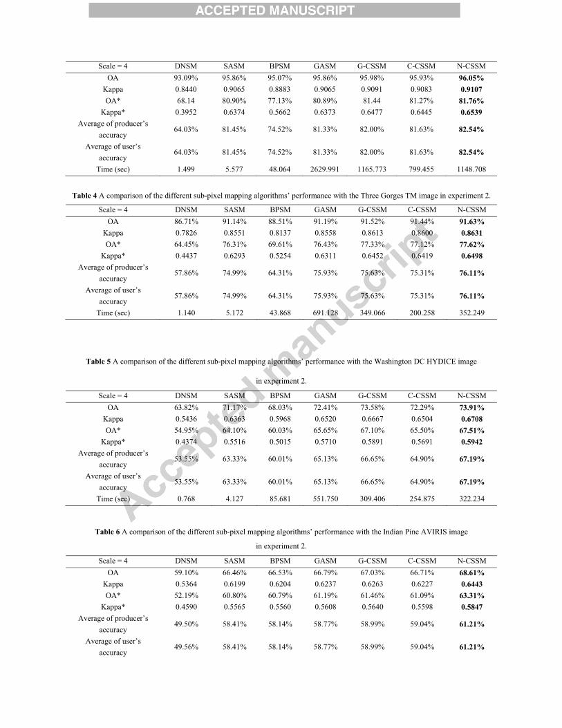
Scale = 4 DNSM SASM BPSM GASM G-CSSM C-CSSM N-CSSM OA 93.09% 95.86% 95.07% 95.86% 95.98% 95.93% 96.05%
Kappa 0.8440 0.9065 0.8883 0.9065 0.9091 0.9083 0.9107 OA* 68.14 80.90% 77.13% 80.89% 81.44 81.27% 81.76%
Kappa* 0.3952 0.6374 0.5662 0.6373 0.6477 0.6445 0.6539 Average of producer’s
accuracy 64.03% 81.45% 74.52% 81.33% 82.00% 81.63% 82.54%
Average of user’s accuracy
64.03% 81.45% 74.52% 81.33% 82.00% 81.63% 82.54%
Time (sec) 1.499 5.577 48.064 2629.991 1165.773 799.455 1148.708
Table 4 A comparison of the different sub-pixel mapping algorithms’ performance with the Three Gorges TM image in experiment 2.
Scale = 4 DNSM SASM BPSM GASM G-CSSM C-CSSM N-CSSM OA 86.71% 91.14% 88.51% 91.19% 91.52% 91.44% 91.63%
Kappa 0.7826 0.8551 0.8137 0.8558 0.8613 0.8600 0.8631 OA* 64.45% 76.31% 69.61% 76.43% 77.33% 77.12% 77.62%
Kappa* 0.4437 0.6293 0.5254 0.6311 0.6452 0.6419 0.6498 Average of producer’s
accuracy 57.86% 74.99% 64.31% 75.93% 75.63% 75.31% 76.11%
Average of user’s accuracy
57.86% 74.99% 64.31% 75.93% 75.63% 75.31% 76.11%
Time (sec) 1.140 5.172 43.868 691.128 349.066 200.258 352.249
Table 5 A comparison of the different sub-pixel mapping algorithms’ performance with the Washington DC HYDICE image
in experiment 2.
Scale = 4 DNSM SASM BPSM GASM G-CSSM C-CSSM N-CSSM OA 63.82% 71.17% 68.03% 72.41% 73.58% 72.29% 73.91%
Kappa 0.5436 0.6363 0.5968 0.6520 0.6667 0.6504 0.6708 OA* 54.95% 64.10% 60.03% 65.65% 67.10% 65.50% 67.51%
Kappa* 0.4374 0.5516 0.5015 0.5710 0.5891 0.5691 0.5942 Average of producer’s
accuracy 53.55% 63.33% 60.01% 65.13% 66.65% 64.90% 67.19%
Average of user’s accuracy
53.55% 63.33% 60.01% 65.13% 66.65% 64.90% 67.19%
Time (sec) 0.768 4.127 85.681 551.750 309.406 254.875 322.234
Table 6 A comparison of the different sub-pixel mapping algorithms’ performance with the Indian Pine AVIRIS image
in experiment 2.
Scale = 4 DNSM SASM BPSM GASM G-CSSM C-CSSM N-CSSM OA 59.10% 66.46% 66.53% 66.79% 67.03% 66.71% 68.61%
Kappa 0.5364 0.6199 0.6204 0.6237 0.6263 0.6227 0.6443 OA* 52.19% 60.80% 60.79% 61.19% 61.46% 61.09% 63.31%
Kappa* 0.4590 0.5565 0.5560 0.5608 0.5640 0.5598 0.5847 Average of producer’s
accuracy 49.50% 58.41% 58.14% 58.77% 58.99% 59.04% 61.21%
Average of user’s accuracy
49.56% 58.41% 58.14% 58.77% 58.99% 59.04% 61.21%

Time (sec) 0.582 3.086 150.267 358.031 244.266 145.141 262.015
Table 7 A comparison of the different sub-pixel mapping algorithms’ performance with the real remote sensing image in experiment
3.
Scale = 8 DNSM SASM BPSM GASM G-CSSM C-CSSM N-CSSM OA 57.05% 57.51% 57.97% 60.47% 60.87% 60.66% 60.86%
Kappa 0.2245 0.2322 0.2414 0.2558 0.2632 0.2593 0.2626 OA* 56.34% 56.81% 57.27% 59.68% 60.09% 59.88% 60.08%
Kappa* 0.1891 0.1972 0.2045 0.2153 0.2231 0.2191 0.2225 Average of producer’s
accuracy 40.05% 40.65% 41.39% 41.39% 41.87% 41.76% 41.85%
Average of user’s accuracy
39.64% 39.88% 40.29% 42.76% 43.33% 43.18% 43.35%
Time (sec) 1.234 5.359 278.648 2809.953 2520.138 548.03 2382.95
Yanfei Zhong received the B.S. degree in information engineering and the Ph.D. degree in photogrammetry and remote sensing from Wuhan University, China, in 2002 and 2007, respectively.
He has been with the State Key Laboratory of Information Engineering in Surveying, Mapping and Remote Sensing, Wuhan University since 2007 and is currently a Professor. His research interests include multi- and hyperspectral remote sensing image processing, artificial intelligence, and pattern recognition. He has published more than fifteen peer-reviewed articles in international journals such as IEEE Transactions on Geoscience and Remote Sensing and IEEE Transactions on Systems, Man and Cybernetics Part B.
Dr. Zhong was the recipient of the National Excellent Doctoral Dissertation Award of China (2009) and New Century Excellent Talents in University of China (2009). He was a Referee of IEEE Transactions on Geoscience and Remote Sensing, IEEE Transactions on Systems, Man and Cybernetics Part B, IEEE Journal of Selected Topics in Applied Earth Observations and Remote Sensing, and Pattern Recognition.
Liangpei Zhang received the B.S. degree in physics from Hunan Normal University, ChangSha, China, in 1982, the M.S. degree in optics from the Xi'an Institute of Optics and Precision Mechanics of Chinese Academy of Sciences, Xi'an, China, in 1988, and the Ph.D. degree in Photogrammetry and Remote Sensing from Wuhan University, Wuhan, China, in 1998.
He is currently with the State Key Laboratory of Information Engineering in Surveying, Mapping and Remote Sensing, Wuhan University, as the head of the Remote Sensing Division. He is also a "Chang-Jiang Scholar" Chair Professor appointed by the Ministry of Education, China. He is currently the Principal Scientist for the China State Key Basic Research Project (2011–2016) appointed by the Ministry of National Science and Technology of China to lead the remote sensing program in China. He is an Executive Member (Board of Governor) of the China National Committee of International Geosphere-Biosphere Programme. He also serves as an Associate Editor of International Journal of Ambient Computing and Intelligence, International Journal of Image and Graphics, International Journal of Digital Multimedia Broadcasting, Journal of Geo-spatial Information Science, and the Journal of Remote Sensing. He has more than 260 research papers and is the holder of 5 patents. His research

interests include hyperspectral remote sensing, high resolution remote sensing, image processing and artificial intelligence.
Dr. Zhang is a fellow of the Institution of Electrical Engineers, an executive Member for the China Society of Image and Graphics, and others. He regularly serves as a Cochair of the series SPIE Conferences on Multispectral Image Processing and Pattern Recognition, Conference on Asia Remote Sensing, and many other conferences. He edits several conference proceedings, issues, and the Geoinformatics Symposiums. He is currently serving as an Associate Editor for the IEEE Transactions on Geoscience and Remote Sensing.
Highlights
� We propose an artificial immune sub-pixel mapping framework for remote sensing imagery.
� The sub-pixel mapping problem is transformed to an optimization problem.
� The proposed algorithm can obtain better sub-pixel mapping results by immune operators.
� Experimental results demonstrate that the proposed approach outperforms the previous methods.

Fig. 1. A raster grid of 3�3 coarse pixels with the scale of 4. (a) An example for the fraction of one land-cover class. (b) The possible
sub-pixel mapping results. (c) The optimal sub-pixel result.
Fig. 2. The mapping between the fraction image and the sub-pixel mapping image.
Fig. 3. Illustration of the initial antibody population (two classes).
Figures 1-10

Fig. 4. The coordinate conversion and the distance calculation between the pixels and sub-pixels.
mutate( ltab )
{ for (j=1 to P) do
if(flip( mp )) j' = j+σNj(0,1) Exchange( ).,. ' j
ltj
lt babbab
end if end for l
tlt abab �*
} Fig. 5. The mutation process.
Fig. 6. A mutation example in CSSM, with the scale of 4.

Fig. 7. The flowchart for the CSSM framework.
Fig. 8. Cauchy and Gaussian density functions.

Fig. 9. The experimental process of the sub-pixel mapping algorithms.

(a) Original artificial image
(960�960)
(b) Original hard classification result
(960�960)
C1
C2
C3
(c) The fraction images (240�240)
(d) DNSM
(e) SASM
(f) BPSM
(g) GASM
(h) G-CSSM
(i) C-CSSM
Zoom for (b)
Zoom for (d)
Zoom for (e)
Zoom for (f)
Zoom for (g)
Zoom for (h)
Zoom for (i)
Zoom for (j)
(j) N-CSSM (k) Zooms for (b) and (d)–(j) C1 C2 C3
Fig. 10. The sub-pixel mapping results in experiment 1 (scale = 4).

(a) Namco TM image
RGB (4,3,2) (1024�1024)
(b) Original hard classification result
(1024�1024)
Water
Vegetation
Snow
Soil
(c) The fraction images (256�256)
(d) DNSM
(e) SASM
(f) BPSM
(g) GASM
(h) G-CSSM
(i) C-CSSM
Zoom for (b)
Zoom for (d)
Zoom for (e)
Zoom for (f)
Zoom for (g)
Zoom for (h)
Zoom for (i)
Zoom for (j)
(j) N-CSSM (k) Zooms for (b) and (d)–(j) Water Vegetation Snow Soil
Fig. 11. The sub-pixel mapping results for the Namco TM image in experiment 2 (scale = 4).
Figures 11-12

(a) Three Gorges TM image RGB
(4,3,2) (400�400)
(b) Original hard classification result
(400�400)
Yangtze River
Lake
Impervious layer
Vegetation
(c) The fraction images (100�100)
(d) DNSM
(e) SASM
(f) BPSM
(g) GASM
(h) G-CSSM
(i) C-CSSM
(j) N-CSSM
Zoom for (b)
Zoom for (d)
Zoom for (e)
Zoom for (f)
Zoom for (g)
Zoom for (h)
Zoom for (i)
Zoom for (j)
(k) Zooms for (b) and (d)–(j) Yangtze river Lake Impervious layer Vegetation
Fig. 12. The sub-pixel mapping results for the Three Gorges TM image in experiment 2 (scale = 4).

(a) Washington DC HYDICE image
RGB (67,27,17) (240�240)
(b) Original hard classification result
(240�240)
roof
road
trail
grass
shadow
tree
(c) The fraction images (60�60)
(d) DNSM
(e) SASM
(f) BPSM
(g) GASM
(h) G-CSSM
(i) C-CSSM
Zoom for (b)
Zoom for (d)
Zoom for (e)
Zoom for (f)
Zoom for (g)
Zoom for (h)
Zoom for (i)
Zoom for (j)
(j) N-CSSM (k) Zooms for (b) and (d)–(j)
Roof Road Trail Grass Shadow Tree Fig. 13. The sub-pixel mapping results for the Washington DC HYDICE image in experiment 2 (scale = 4).
Figures 13-14
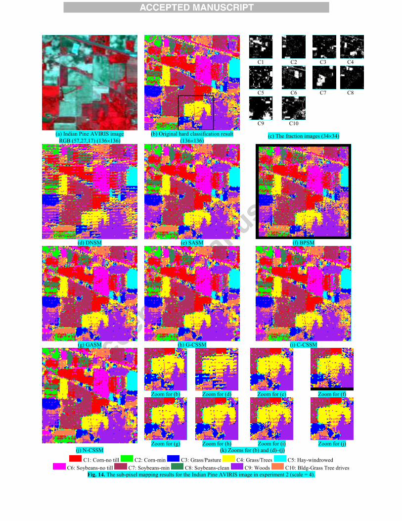
(a) Indian Pine AVIRIS image
RGB (57,27,17) (136�136)
(b) Original hard classification result
(136�136)
C1
C2
C3 C4
C5
C6
C7 C8
C9
C10
(c) The fraction images (34�34)
(d) DNSM
(e) SASM
(f) BPSM
(g) GASM
(h) G-CSSM
(i) C-CSSM
Zoom for (b)
Zoom for (d)
Zoom for (e)
Zoom for (f)
Zoom for (g)
Zoom for (h)
Zoom for (i)
Zoom for (j)
(j) N-CSSM (k) Zooms for (b) and (d)–(j)
C1: Corn-no till C2: Corn-min C3: Grass/Pasture C4: Grass/Trees C5: Hay-windrowed C6: Soybeans-no till C7: Soybeans-min C8: Soybeans-clean C9: Woods C10: Bldg-Grass Tree drives
Fig. 14. The sub-pixel mapping results for the Indian Pine AVIRIS image in experiment 2 (scale = 4).

(a) Shenzhen IKONOS image (784�240)
(b) Shenzhen ETM image RGB (4,3,2) (98�30)
(c) Shenzhen IKONOS classification marker image
Bare soil
Vegetation
Water
City
(d) The fraction images of the ETM image (98�30)
(e) DNSM
(f) SASM
(g) BPSM
(h) GASM
(i) G-CSSM
(j) C-CSSM
(k) N-CSSM
Bare soil Vegetation Water City
Zoom for (b)
Zoom for (e)
Zoom for (f)
Zoom for (g)
Zoom for (h)
Zoom for (i)
Zoom for (j)
Zoom for (k)
(l) Zooms for (b) and (e)–(k) Fig. 15. The sub-pixel mapping results for the Shenzhen ETM image in experiment 3 (scale = 8).
Figures 15-17
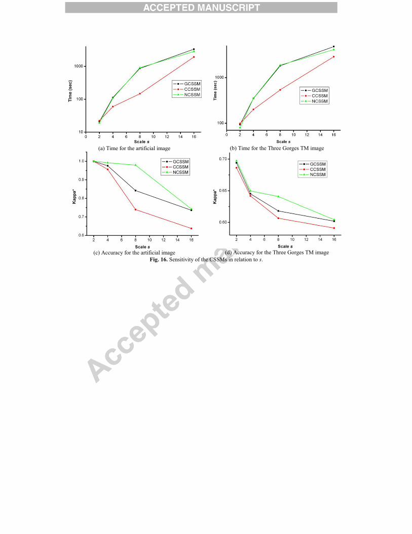
(a) Time for the artificial image
(b) Time for the Three Gorges TM image
(c) Accuracy for the artificial image
(d) Accuracy for the Three Gorges TM image
Fig. 16. Sensitivity of the CSSMs in relation to s.

(a) G-CSSM (NB = 20)
(f) C-CSSM (NB = 20)
(k) N-CSSM (NB = 20)
(b) G-CSSM (NB = 40)
(g) C-CSSM (NB = 40)
(l) N-CSSM (NB = 40)
(c) G-CSSM (NB = 60)
(h) C-CSSM (NB = 60)
(m) N-CSSM (NB = 60)
(d) G-CSSM (NB = 80)
(i) C-CSSM (NB = 80) (n) N-CSSM (NB = 80)
(e) G-CSSM (NB = 100)
(j) C-CSSM (NB = 100)
(o) N-CSSM (NB = 100)
G-CSSM C-CSSM N-CSSM Fig. 17. Sensitivity of the CSSMs in relation to the three parameters for the Three Gorges TM image.