Embed Size (px)
Citation preview

ASSEMBLY LINE REBALANCING WITH NON-CONSTANT TASK TIME
ATTRIBUTE
by
YUCHEN LI
A dissertation submitted to the
Graduate School-New Brunswick
Rutgers, The State University of New Jersey
In partial fulfillment of the requirements
For the degree of
Doctor of Philosophy
Graduate Program in Industrial and Systems Engineering
written under the direction of
Thomas Boucher
And approved by
_______________________________
_______________________________
_______________________________
_______________________________
_______________________________
_______________________________
New Brunswick, New Jersey
OCTOBER, 2016

ii
ABSTRACT OF THE DISSERTATION
ASSEMBLY LINE REBALANCING WITH NON-CONSTANT TASK TIME
ATTRIBUTE
By YUCHEN LI
Dissertation Director:
Thomas Boucher
Assembly line has been widely used in producing complex items, such as
automobiles and other transportation equipment, household appliances and electronic
goods. Assembly line balancing is to maximize the efficiency of the assembly line so that
the optimal production rate or optimal length of the line is obtained. Since the 1950s there
has been a plethora of research studies focusing on the methodologies for assembly line
balancing. Methods and algorithms were developed to balance an assembly line, which is
operated by human workers, in a fast and efficient fashion. However, more and more
assembly lines are incorporating automation in the design of the line, and in that case the
line balancing problem structure is altered. For these automated assembly lines, novel
algorithms are provided in this dissertation to efficiently solve the automated line balancing
problem when the assembly line includes learning automata.

iii
Recent studies show that the task time can be improved during production due to
machine learning, which gives the opportunities to rebalance the assembly line as the
improvements occur and are observed. The concept of assembly line rebalancing or task
reassignment are crucial for the assembly which is designed for small volume production
because of the demand variation and rapid innovation of new product. In this dissertation,
two forms of rebalancing are provided, forward planning and real time adjustment. The
first one is to develop a planning schedule before production begins given the task time
improvement is deterministic. The second one is to rebalance the line after the
improvements are realized given the task time improvement is random. Algorithms address
one sided and two sided assembly lines are proposed. Computation experiments are
performed in order to test the performance of the novel algorithms and empirically validate
the merit of improvement of production statistics.

iv
ACKNOWLEDGEMENT
The dissertation “assembly line rebalancing with non-constant task time attribute”
concludes my career as a Ph.D. student at Rutgers University. It is a great journey that I
could never imagine I have finished in such an amazing way. Not only the unanimous
passes but also the greatest ever compliments receiving from all committee members of
my defense do make me feel all the gritty effort of the past four years finally starts paying
off.
My beloved parents, Jin Li and Shangtao Ding provide me untiring, unconditional
supports which lead me this far. There are no words to describe how important they are to
me. I am so grateful to be their son.
My adviser, Dr. Thomas Boucher, who has been inspiring me from day 1 when I
got into the ISE program. He opened the door of my research and help me clean all of the
road bumps on the path of completing the dissertation. Thank you, Mr. big picture, I am
grateful to be your apprentice.
Now, my friends, who sit tight in the cheering section offering me everything they
could possibly offer when I am in dire need. Youhu Zhao comforted me and shared his
experience when I hit my bottom and could not escape the trough on my own. Chengguang
Lu, Ching Wong, and Yi Zhang are always there to soothe the pain of my loneliness when
I need company. Also, special thanks to ChuanChuan (Caroline), who taught me to become
a tough person, which I think will benefit me in the future. I am grateful to be your lifelong
friends.

v
I also appreciate my committee members, Sanchoy Das, Susan Albin, Honggang
Wang, David Coit, and David Nembhard for their invaluable advice on how to shape the
dissertation crystal clear and rock solid.
Ultimately, I wish the dissertation would provide the readers a whole new
perspective to the line balancing area. I also ask for your forgiveness in advance for any
inaccurate and insufficient statements I made throughout my dissertation.
Yuchen Li at
Library of Science and Medicine café lounge
09/12/2016

vi
TABLE OF CONTENT
ABSTRACT OF THE DISSERTATION ....................................................................... ii
ACKNOWLEDGEMENT ............................................................................................... iv
TABLE OF CONTENT ................................................................................................... vi
LIST OF FIGURES ......................................................................................................... xi
LIST OF TABLES ......................................................................................................... xiii
1. Introduction ............................................................................................................... 1
1.1 Traditional flow assembly line............................................................................ 1
1.2 Automated Flexible Assembly Line ................................................................... 3
1.3 Motivation ........................................................................................................... 5
1.4 Notations ............................................................................................................. 7
1.5 Assembly Line Balancing Problem .................................................................... 9
1.5.1 SALBPF......................................................................................................... 12
1.5.2 SALBP1 ......................................................................................................... 12
1.5.3 SALBP2 ......................................................................................................... 14
1.5.4 SALBPE......................................................................................................... 15
1.5.5 TALBP1 ......................................................................................................... 15
1.5.6 Forward Planning for SALBP1 under dynamic task attributes .................... 15
1.5.7 Task reassignment for SALBP2 under non-constant task attributes ............ 18
1.6 Summary ........................................................................................................... 19

vii
2. Literature review .................................................................................................... 21
2.1 Literature Review on data structure and complexity ........................................ 21
2.1.1 Data structure ............................................................................................... 21
2.1.2 Complexity of data set ................................................................................... 22
2.2 An overview of algorithms addressing SALBP ................................................ 23
2.3 Literature Review on Dynamic Programming .................................................. 24
2.4 Literature Review of the Branch and Bound procedure in Assembly Line
Balancing ...................................................................................................................... 26
2.4.1 Lower bounds ................................................................................................ 27
2.4.2 Dominance rules ........................................................................................... 29
2.4.3 Branch and Bound procedure on SALBP1 ................................................... 30
2.4.4 Branch and Bound procedure on SALBP2 ................................................... 33
2.5 Literature Review on Priority-based methods .................................................. 36
2.6 Literature Review on task attributes ................................................................. 38
2.6.1 Dynamic task attributes ................................................................................ 39
2.6.2 Uncertain task attributes............................................................................... 40
2.6.3 Recent research on ALBP considering non-constant task attribute ............. 40
2.7 Summary ........................................................................................................... 42
3. Simple Assembly Line Balancing Problem-1 with dynamic task time attribute
43
3.1 Conventional BnB procedure ............................................................................ 43
3.2 Line rebalancing schedule ................................................................................. 44

viii
3.3 Backward induction algorithm .......................................................................... 44
3.4 Computational experiments .............................................................................. 50
3.4.1 Backward Induction (weak) and Conventional Algorithm ........................... 50
3.4.2 Backward Induction (Strong) and Conventional algorithm ......................... 54
3.5 Case study ......................................................................................................... 55
3.6 Summary ........................................................................................................... 61
4. Simple Assembly Line Balancing Problem-2 with non-constant task time
attribute ........................................................................................................................... 63
4.1 Rebalancing schedule with non-constant task time attributes .......................... 63
4.2 A BnB based exact solution procedure to solve SALBP2 with non-constant task
time 66
4.2.1 A conventional algorithm .............................................................................. 66
4.2.2 ENCORE ....................................................................................................... 67
4.2.3 An illustrative example ................................................................................. 71
4.2.4 The comparison between the conventional solution and ENCORE.............. 74
4.2.5 Computational experiment ............................................................................ 76
4.3 Design of Experiments ...................................................................................... 78
4.3.1 Components of an experiment ....................................................................... 79
4.3.2 Pretest ........................................................................................................... 80
4.3.3 One sample t test ........................................................................................... 83
4.4 Summary ........................................................................................................... 86
5. Priority rules-based algorithmic design on two sided assembly line balancing 87

ix
5.1 The investigation of PRBMs in TALBP ........................................................... 87
5.1.1 Application of elementary rules .................................................................... 88
5.1.2 Application of composite rules...................................................................... 93
5.2 Algorithmic design with BDP ........................................................................... 95
5.2.1 Enumeration of states ................................................................................... 96
5.2.2 Solution space reduction approaches ........................................................... 97
5.2.3 The application of PR_BDP.......................................................................... 99
5.2.4 Design of Experiments ................................................................................ 102
5.3 Summary ......................................................................................................... 104
6. Summary ................................................................................................................ 106
References ...................................................................................................................... 111
Appendix A: Benchmark data sets .............................................................................. 118
Appendix B: The basic flow chart of ENCORE ......................................................... 132
Appendix C: Computational tests for backward induction algorithm .................... 133
Appendix D: Case study ............................................................................................... 144
Appendix E: Computational tests for ENCORE ....................................................... 146
Appendix F: Design of Experiments (ENCORE) ....................................................... 164
Appendix G: Performance of elementary rules ......................................................... 168
Appendix H: Performance of enhanced elementary rules ........................................ 177
Appendix I: Performance of the composite rules....................................................... 183

x
Appendix J: Performance of the priority-based bounded dynamic programing ... 187
Appendix K: Design of Experiments (PR_BDP) ........................................................ 191

xi
LIST OF FIGURES
Figure 1 Basic structure of two-sided assembly line .......................................................... 2
Figure 2 Learning the peg-into-hole assembly operation Left: evolution of the insertion
time. Right: evolution of the average quality based on the contact forces (Source:
Nuttin and Von Brussel, 1999) ............................................................................... 4
Figure 3 Error rate per attribute value versus the number of examples [Source: Lopes and
Camarinha-Matos(1995)] ........................................................................................ 5
Figure 4 Precedence graph of SALBP ................................................................................ 9
Figure 5 Precedence graph of TALBP .............................................................................. 11
Figure 6 Sample assignment of the example problem ...................................................... 11
Figure 7 Task reassignment procedure ............................................................................. 17
Figure 8 Simple solution to SALBP with cycle time 9 ..................................................... 26
Figure 9 Example for BnB procedure for SALBP1 .......................................................... 31
Figure 10 Tree structural solution for SALBP1 (DFS) ..................................................... 32
Figure 11 Tree structural solution for SALBP1 (SALOME1).......................................... 33
Figure 12 Tree structural solution for SALBP2 (SALOME2).......................................... 36
Figure 13 12 Tasks two sided assembly line .................................................................... 38
Figure 14 Illustrative Case Study System Architecture .................................................... 56
Figure 15 Actions in the rebalancing process ................................................................... 59
Figure 16 Task reassignment schedule for b=1000 .......................................................... 61
Figure 17 Task reassignment under the dynamic task time attribute ................................ 64
Figure 18 Task reassignment under uncertain and discrete task time improvements ....... 65

xii
Figure 19 The solution structure to a simple SALBP2 problem with non-constant task time
and a lot size of to 30 ............................................................................................ 66
Figure 20 Simple example. Top: original problem. Bottom: new problem ...................... 73
Figure 21 Solution of the original problem (optimal cycle time=9) ................................. 74
Figure 22 Line-oriented cycle time adjustment procedure (current upper bound=8.5) .... 74
Figure 23 Station-oriented cycle time adjustment procedure (optimal cycle time=8)...... 74
Figure 24 Relationship between p value and improvement (Spline interpolation is used to
find the boundary) ................................................................................................. 86
Figure 25 The enumerative procedure of elementary PRBMs ......................................... 89
Figure 26 Top: 4 task data set; Middle: Solution 1; Bottom: Solution 2 .......................... 91
Figure 27 Number of best solutions of composite rules in relation to the weight of F .... 95
Figure 28 Structure of PR_BDP ....................................................................................... 99
Figure 30 Precedence graph of Mansoor's data set ......................................................... 118
Figure 31 Precedence graph of Heskiaoff's data set ....................................................... 118

xiii
LIST OF TABLES
Table 1 Notations ................................................................................................................ 8
Table 2 Taxonomy of SALBP .......................................................................................... 10
Table 3 The precedence matrix for the example of Figure 4 ............................................ 22
Table 4 Processing time and tails of Figure 4 ................................................................... 29
Table 5 The performance of algorithms on Mansoor's data set (Mansoor,1964, cycle time
is 48)...................................................................................................................... 51
Table 6 The performance of algorithms on Heskiaoff's data set (Heskiaoff,1968, cycle time
is168)..................................................................................................................... 52
Table 7 The performance of algorithms on Scholl's (Figure 4) data set (cycle time is 10).
............................................................................................................................... 53
Table 8 The performance of algorithms on Mansoor's data set (cycle time is 48) ........... 54
Table 9 The performance of algorithms on Heskiaoff's data set (cycle time is 168)........ 54
Table 10 The performance of algorithms on Scholl's (Figure 4) data set (cycle time is 10)
............................................................................................................................... 55
Table 11 Production statistics ........................................................................................... 60
Table 12 Computational performance between algorithms in Heskiaoff's data set (n=28)
given m=8 ............................................................................................................. 77
Table 13 Computational performance between algorithms in Kilbrid's data set (n=45) given
m=8 ....................................................................................................................... 77
Table 14 Computational performance between algorithms in Arcus's data set (n=83) given
m=8 ....................................................................................................................... 78
Table 15 Summary statistics for each t test on response comparisons (Eq. 26) ............... 84

xiv
Table 16 p value matrix for each t test .............................................................................. 85
Table 17 Average performance of the elementary rules ................................................... 90
Table 18 p values of paired t tests of Avg_dev of elementary rules (95% confidence level)
............................................................................................................................... 90
Table 19 Average performance of the elementary rules with two principles ................... 92
Table 20 p values of paired t tests of Avg_dev of elementary rules with and without two
principles (95% confidence level) ........................................................................ 92
Table 21 The scaled factor for the application of composite rules ................................... 93
Table 22 Average performance of the best weighted combinations for each pairing of rules
............................................................................................................................... 94
Table 23 The number of best solutions of each weighted pairing rules out of 34 cases as
measured by Avg_dev........................................................................................... 94
Table 24 Comparisons of performance between best PRBMs and PR_BDP ................. 100
Table 25 Comparisons between the best NM reported and best NM generated by PR_BDP
............................................................................................................................. 100
Table 26 Summary statistics for percent reduction in Avg_NM of 34 basic data instances
............................................................................................................................. 103
Table 27 Summary statistics for percent reduction in Avg_I of 34 basic data instances 103
Table 28 Summary of Algorithms .................................................................................. 108

1
1. Introduction
1.1 Traditional flow assembly line
Flow assembly line is an important process in the manufacturing ecosystem. It is
commonly used to produce automobiles, transportation equipment, household appliances and
electronic goods. The emergence of the assembly line can be traced back to the 19th century and
the first flow assembly line was initiated to produce the steam engines at the factory of Richard
Garrett & Sons in 1853. Henry Ford is mostly renowned for his contribution to the rise of mass
production in the early 20th century. The assembly line developed for the Ford Model T began
operation on December 1, 1913. It had immense influence on the world. In the 1950s, engineers
started to experiment with robots in the assembly line as a means of industrial development.
Robots have proved to be faster, more cost effective in high wage countries, and more accurate
than humans. From late 20th century to the present, with developments in computer science, the
innovation of the assembly line reaches a new level where computer programs and algorithms
intelligently automate the production process. It gives birth to some novel assembly line systems,
such as assembly lines with supervisory control and learning.
The assembly line designs that we address in this thesis can be categorized into the one
sided line (OAL) and the two sided line (TAL). For OAL, the assembly line consists of a number
of workstations arranged along a transportation device, i.e. conveyer belt, which moves the part
(jobs) at same speed in order to pace the line. The speed is determined by a cycle time. The parts
are consecutively launched from top to bottom of the line and assembled in workstations after
certain operations (tasks) have been done in a certain amount of time. The total sojourn time for a
part staying at a workstation should not exceed the cycle time of the assembly line. In order to
perform a particular task, machines and workers with certain skills are required in each

2
workstation. Furthermore, tasks are dependent on each other and the relationships are often
characterized in a precedence graph.
For TAL, as opposed to OAL, where workers can only access the tasks from one side of
the line, workers can perform the tasks cooperatively from both sides of the line. The basic
structure of TAL can be seen in Figure 1. Along the assembly line, there are several positions
where parts are processed independently. In each position, there are two stations called mated-
stations which are located at different sides of the line. Each mated station is attended by a worker
or a robot. Thus, each mated station can work independently. The speed of the line is determined
by the cycle time which is the sojourn time of the part in each position. As distinct from OAL,
where tasks have two attributes (task times and precedence relations between tasks) the task in
TAL has a third attribute which is the operational direction. An individual task can be assigned to
either side of the line or only to one side of the line based on the operational direction (left, right
or either).
Figure 1 Basic structure of two-sided assembly line

3
The goal of designing an assembly line is to maximize its production efficiency (E)
measured by the product of the cycle time and the number of stations (or positions for TAL) in the
assembly line. Mathematically, the efficiency can be quantified by Eq. (1). The assembly line is
balanced when the maximal efficiency is achieved.
1 (1)
: the number of stations
: cycle time of the line
Em c
m
c
1.2 Automated Flexible Assembly Line
A Highly automated and flexible assembly system brings with it its own set of particular
characteristics. Two emerging characteristics that are important to discuss in the context of this
thesis are 1) machine learning or learning automata and 2) control architecture and collaborative
learning.
It has been shown that robots, as intelligent agents, are able to improve their performance
on given tasks. Such improvements result from encoding learning algorithms in the control
programs of the agents. For example, Nuttin and von Brussel (1999) have shown that a neural net
controller with reinforcement learning can improve the task performance time. They studied the
classic “peg-in-a-hole” insertion problem and found that both the insertion time and the amount of
contact force required for the insertion (referred to as force quality) improved over the number of
executions of the task as shown in Figure 2. The characteristic non-linear relationship between
insertion time and the number of insertions attempted is typical of a learning curve function.

4
Figure 2 Learning the peg-into-hole assembly operation Left: evolution of the insertion
time. Right: evolution of the average quality based on the contact forces (Source: Nuttin
and Von Brussel, 1999)
Lopes and Camarinha-Matos (1995) illustrated another aspect of learning in flexible
assembly systems. In their work they focus on the detection of errors in the robot assembly task
and the design of recovery from error and prevention of reoccurrence of the same errors over time.
The improvement comes as a result of building a knowledge base of models for monitoring,
diagnosis and recovery through machine learning. In their experiment they study the operation of
a pick and place robot. By introducing examples of abnormal conditions they study the sizes of
the machine learning branching tree necessary to produce good results in diagnosing and reducing
the error rates as shown in Figure 3.

5
Figure 3 Error rate per attribute value versus the number of examples [Source: Lopes and
Camarinha-Matos(1995)]
1.3 Motivation
The two examples show the existence of non-constant task time for the robots when the
supervisory control and learning automata are involved. The task time decreases at the beginning,
and then approaches a constant (plateau) after producing a number of units, which is the production
ramp-up period. In traditional assembly line balancing, for large size production, the line is
balanced once based on standard time, which is the constant task time that is reached after the
production ramp up period. However, this is not applicable to small batch production where the
production is still in the ramp-up period. This gives the motivation for considering rebalancing
the station configurations as a means to reduce the cycle time in each production cycle, i.e.
dynamic reassigning of the tasks to workstations. Task reassignment is very common in mixed-
model assembly lines in which a common task of different product models can be assigned to
different workstations in different production cycles (Boysen et al., 2012). Cost related to task
reassignment, e.g. station setup cost and training cost, has to be considered in the optimization
Number of examples

6
process (Bukchin et al.,2006). However, such cost is negligible in the framework of an automated
flexible assembly line when the robot in each station is assumed to be multifunctional, and
knowledge regarding the task time improvement can be perfectly shared between robots and
workstations. Indeed, Angerer et al. (2010) have demonstrated self-reconfiguration of mobile
robots in car manufacturing, including the transfer of skills among robots. Therefore, it may be
economic as well as efficient to rebalance the assembly line considering the non-constant task
time.
A fundamental difference exists in learning as between an automated assembly line and a
worker assembly line. If a task is reassigned among workers, the reduction in the task time is lost
because the task skill achieved by one worker cannot be transferred to another worker. In an
automated system, such as that which we describe, the improvement is preserved by the
supervisory controller that oversees the assembly line and the learned skill (information) can be
transferred to other agents on the line.
As such, there is a demand to revisit the classic problem with dynamic task time attribute
incorporated. More importantly, fast and efficient algorithms must be provided in order to serve
the purpose of rapid responses along the automated assembly system in small batch size
production. We study two ways to satisfy the requirement: forward planning and real-time
adjustment. As for forward planning, we assume that the pattern of the task time developing in
batches is deterministic and assembly line balancing schedule is generated before the production
process begins. Once the task times change, there is always an optimal solution at hand to adjust
the task assignment as a means to rebalance the assembly line. As for real-time adjustment, the
pattern of task time evolution is stochastic or random, which requires an instantaneous response
after the changes of the task times are observed. In such a situation, an efficient algorithm is

7
necessary to rebalance the assembly line during production. Hence, the objective of this
dissertation is to propose methods and algorithms to address the aforementioned problems from
the perspectives of planning and real-time adjustment schemes.
1.4 Notations
The following notations are used throughout the paper. The definitions are as follows in
Table. 1. Some variables are specific to TAL or OAL which are specified in the parenthesis after
the variable definition, and the other variables are used in general.

8
Table 1 Notations
`
Variable names
c
n
t v
m
m*
z
m i
m i *
P
t min , t max , t sum
t vi:
c*
c i
c i *
c i '*
ctemp
N
V
V*
Vk
V i
V i *
NM
NS
TdL v
TdS v
L v
El v
F v
S v
GLB (GUB )
LB (UB )
LBs (UBs )
Task time at production cycle i , v =1...n , i =1,...z
Descriptions
Cycle time of the line
Number of tasks
Task processing times, v =1…n
Number of stations (OAL)
Optimal number of stations (OAL)
Batch size
Number of stations at production cycle, i =1....z (OAL)
Optimal number of stations at production cycle i , i =1...z (OAL)
Precedence matrix, P(v,o)=1 iff task v is the direct predecessor of task o .
Minimum , maximum and total task times
Task v processing time divided by latest position
Optimal cycle time of the line (OAL)
Cycle time of the line at production cycle i , i =1,...z (OAL)
Optimal cycle time of the line at production cycle i considering task reassignment, i =1,...z (OAL)
A feasible task sequence (OAL)
Optimal task sequence (OAL)
Optimal cycle time of the line at production cycle i without task reassignment, i =1,...z (OAL)
Total prodution quantities
Temporary upper bound of cycle time during the implementation of ENCORE
A feasible task assignment at station k , k =1,...m (OAL)
A feasible task sequence at production cycle i , i =1,...z (OAL)
Optimal task sequence at production cycle i , i =1,...z (OAL)
Total number of positions (TAL)
Total number of workstations (TAL)
Intermediate lower (upper) bound
Set of intermediate lower (upper) bounds of NM for all developing solutions
Task v processing time divided by slack
Latest possible position to which task v can be assigned (TAL)
Earliest possible position to which task v can be assigned (TAL)
Total number of followers of task v
Priority score of task v
Global lower (upper) bound
(2)
(3)

9
1.5 Assembly Line Balancing Problem
The assembly line balancing problem can be subdivided into simple assembly line
balancing (SALBP) and two sided assembly line balancing (TALBP). They correspond to OAL
and TAL respectively.
There are two constraints in SALBP, precedence and station cycle time constraints. Firstly,
the precedence constraints are always represented in a precedence graph, as shown in Figure 4. A
task can only be assigned after all of its predecessors are assigned. For instance, in Figure 4, task
5 is available to assign when both task 1 and 4 have been assigned. Secondly, the total task time
of one station cannot exceed the cycle time of the line. The following terms are useful to describe
the task assignment in relation to constraints.
The task is available when all preceding tasks have been assigned
The task is assignable to a station when the total task time of that station does not exceed
the cycle time c after the task is assigned.
The load of the station is maximal if no further assignable tasks exists.
The bottleneck station is the station whose total task time is the highest among all stations
Figure 4 Precedence graph of SALBP

10
The traditional assembly line balancing problem is categorized into four types according
to different inputs and objectives, as are shown in Table. 2.
Table 2 Taxonomy of SALBP
number of station(m)
cycle
time(c) Given Minimize
Given SALBPF SALBP1
Minimize SALBP2 SALBPE
Similar to SALBP, TALBP also has four types (TALBPF, TALBP1, TALBP2 and
TALBPE). The precedence graph of TALBP for an example problem is shown in Figure 5. The
task number is stored inside the node. There are two pieces of information stored in the parenthesis
associated with each node. The first element is referred to the task time, and the second element
designates the sides to which the task can be assigned. The precedence relations between tasks are
described in the acyclic graph. For instance, task 3, which requires 1 unit of time to perform and
can only be assigned to the right side of the line, has one predecessor (task 1) and one successor
(task 5). Each side of a position is attended by one worker or robot doing the tasks assigned to
that position/side.
Compared with SALBP, TALBP has an additional characteristic—Delay. We illustrate it
with an example. A sample assignment of the problem described in Figure 5 is shown in Figure 6.
As can be seen, there are two sources of idle time, namely, remaining capacity and delay. The first
source is a common source which occurs in SALBP as well. It indicates that there is no room for
the available task with the smallest task time to be assigned. So, if the target cycle time is 5, the
example allows that only 4 time units of work can be assigned at position 1. Therefore, there is

11
some unused capacity. The second source is TALBP specific, it occurs as a task cannot be
performed immediately after its previous task in the same station is finished. For instance, in Figure
6, after task 2 is done, task 4 cannot be performed until his predecessor task 1 is finished on the
other mated-station. In other words, task 1 creates a mirror image on the other mated-station, and
a delay occurs as the end time of the mirror image is later than that of the previous task (task 2)
within the station.
Figure 5 Precedence graph of TALBP
Figure 6 Sample assignment of the example problem
The TALBP is subject to three constraints: cycle time, precedence and operational
constraints. The cycle time constraint requires that the finish time of the last task in a station should

12
be smaller than the cycle time. In SALBP, the finish time of the last task is always equal to the
total load of the station, which is the sum of the task times at that station. In TALBP, however, the
finish time of the last task is always greater than or equal to the total load of the station because
of the delay. The precedence constraint states that a task can be assigned only if all of its
predecessors have been finished meaning that the beginning time of a task shall be later than the
latest end time of its predecessors. In comparison to the precedence constraint, which only
considers whether all predecessors are assigned, the precedence constraint in TALBP takes
account of the end time of the predecessors at both mated-stations. The operational constraint
guarantees that the task is performed on its designated side.
1.5.1 SALBPF
SALBP-F is a problem which is to establish whether or not a feasible line layout exists for
a given combination of m and c. For the example of Figure 4, a feasible sequence of m=7 and c=10
is V1={1}, V2={3,4}, V3={5,6}, V4={2,7}, V5={8}, V6={9}, V7={10}. This is a NP-complete
problem which means no polynomial time solution is known. That is to say, the time required to
solve the problem using any currently known algorithm increases very quickly as the size of the
problem grows. Hence, whether the problem can be solved in polynomial time depends on the
complexities of the problem structure, which will be discussed in the literature review of Chapter
2.
1.5.2 SALBP1
SALBP1 is the most common problem among all versions of the assembly line balancing
problem. The objective is to minimize the number of stations for a given cycle time. Equivalently,

13
the length of the assembly line and the amount of resources are minimized when the number of
stations is minimized. Solving the problem is very sophisticated due to many possible station
configurations. Indeed, it a NP-Hard problem meaning that solving it in polynomial time is
impossible and the solution time is impractical as the size of the problem is relatively large.
Mathematically, the SALBP1 line balancing problem can be formulated as follows (Otto and Otto,
2014).
1
1
1 if task v is assigned to station k
0 otherwise
. .
1 1... (4)
, if (
vk
m
vk
k
m
vk ok
k
Min m
Decision Variables
x
s t
x v n
k x k x P
1
1
v,o) 1 , 1... (5)
1.... (6)
m
k
n
vk v
v
v o n
x t c k m
Constraint (4) is the indivisible constraint, it ensures that a task can only be assigned to one
workstation; constraint (5) is the precedence constraint, it ensures that a task is only available to a
station if and only if all of its predecessors have been assigned; constraint (6) is the speed
constraint, it ensures that the tasks at each station of the assembly line can be completed within the
cycle time of the line, i.e. the line is paced. It is worth noting that the constraints are identical
regardless of the problem types.
The optimal solution of the example in Figure 4 is m=6 given cycle time c= 10. The
associated station configuration is V1={3,4}, V2={1,5}, V3={2,7}, V4={6,8}, V5={9}, V6={10}.

14
1.5.3 SALBP2
SALBP2 is a problem that aims to minimize the cycle time of the assembly line for a given
m. The cycle time serves as a bound for each workstation and guarantees the line is paced.
Moreover, the cycle time is a measure of the productivity of the line. The smaller the cycle time
is, the more productive the assembly line will be. It is a dual problem of SALBP1, because
SALBP2 minimizes c given a fixed m, while SALBP1 minimizes m given c. Like the SALBP1,
SALBP2 also falls into the category of NP-Hard problem. The problem can be formulated as
follows.
1
1
1 if task v is assigned to station k
0 otherwise
. .
1 1... (7)
, if (
vk
m
vk
k
m
vk ok
k
Min c
Decision Variables
x
s t
x v n
k x k x P
1
1
v,o) 1 , 1... (8)
1.... (9)
m
k
n
vk v
v
v o n
x t c k m
Given the number of stations m = 5, the optimal solution of the example in Figure 4 is
c=11. The associated station configuration is V1={3,4}, V2={1,5}, V3={2,7}, V4={6,8}, V5={9,10}.

15
1.5.4 SALBPE
SALBPE is a more general problem than previous three problems. It is to maximize the
efficiency (cf. Section 1.1) of the assembly line by making tradeoffs between minimizing the
number of stations and cycle time considering their interrelationships. However, this problem is
not as popular as the SALBP1 and SALBP2 because adjusting two variables at the same time is
not very practical and sometimes one variable is more attractive than another in industrial
problems. Generally speaking, it could be solved by iteratively solving the SALBP1 or SALBP2.
1.5.5 TALBP1
TALBP1 is a more common problem than the other three problems of TALBP in the
literature. It is to minimize the number of positions of the assembly line with a fixed cycle time.
Because of the additional constraints and the impact of the delay time, it is a more complex
problem than SALBP1. Hence, it is a NP-Hard problem as well. Because of its complexity,
heuristics and meta-heuristics are always employed to find a good solution in a reasonable amount
of time. These methods are introduced in the literature review section. Further, in this dissertation,
priority rules- based methods (PRBMs) as well as a bounded dynamic programming (BDP) scheme
are proposed to solve the TALBP1 by exploiting the problem specific knowledge.
1.5.6 Forward Planning for SALBP1 under dynamic task attributes
As mentioned before (cf. Section 1.3), there is an existing yet unsolved problem: Dynamic
task reassignment under changing task performance times. Task time reduction could be achieved
by improvement induced by human or technology in terms of the cumulative proficiency of skills
or process innovation. Task reassignment becomes possible in modern assembly systems. For
example, the assembly line with supervisory control is capable of changing the production process

16
between production cycles (repetitions). The supervisory machine will dispatch orders (changes)
to the machines in the workstations, and the adjustment will be made accordingly.
A problem arises when the current task assignment may not be optimal given a change in
the dynamic task time attribute and the number of workstations can be reduced while maintaining
the desired cycle time. Otto and Otto (2014) provides the solution procedures considering the
dynamic attributes of task time, when task reassignment is not allowed during the learning period.
In this dissertation, we aim to optimize the configuration of the assembly line by considering
reassigning the tasks in each production cycle as task times are reduced. Figure 7 illustrates the
decision making process given a batch size of 30. At the beginning, an optimal solution consisting
of the number of stations (m(1)) and the task arrangement (V(1)) are obtained for the first
production cycle. Then, as production cycle increases and task time falls according to a learning
function, the current solution is no longer optimal at the uth production cycle. A new solution set
(m(u), V(u)) has to be searched. Hatched area implies the optimality of solution (m(1), V(1) is
maintained from the first production cycle to the (u-1)th production cycle. The above procedure is
repeated until the solution to last repetition is found (m(30), V(30)). Generally speaking, for the
batch size z, the problem we are addressing for SALBP1 can be formulated as follows:

17
1
1
1 if task v is assigned to station k at the ith repetition
0 otherwise
. .
1 1... , 1...z (1
z
i
i
i
vk
mi
vk
k
Min m
Decision Variables
x
s t
x v n i
1 1
1
0)
, if (v,o) 1 , 1... (11)
1.... , 1...z (12)
m mi i
vk ok
k k
ni i
vk v
v
k x k x P v o n
x t c k m i
Figure 7 Task reassignment procedure

18
Our interest is to develop a smart algorithm that will tell us whether or not a new solution
is required or whether the current solution is still valid. If the problem could be reduced to
determine whether the optimal solution to the current batch is still optimal, the computational effort
can be reduced. When a current configuration is no longer optimal, tasks will be dynamically
reassigned to stations based on the new optimal design. In automated flexible assembly systems
this simply means that the tasks are dynamically reassigned among fewer robots without loss of
the information that has led to reduced assembly task times. Robots (agents) that are no longer
required in the current assembly configuration can be released for work in other parts of the plant,
or on other assemblies, thus maximizing the efficient use of machines. To tackle this problem, a
novel algorithm is proposed in this paper concerning task reassignment based on dynamic task
assembly times where the learning rate is predetermined. As a result, a planning schedule for the
design of the assembly line is generated upfront before production begins in order to better allocate
the resources. Comparisons are made with the use of the standard algorithms currently in the
literature in terms of the performance.
1.5.7 Task reassignment for SALBP2 under non-constant task attributes
The presence of non-constant task time attribute also provides opportunities for further
reducing the cycle time in SALBP2. At times, it is more convenient to adjust the task assignment
than to reduce the number of stations. Moreover, the pattern by which the task time progresses
could be deterministic or uncertain. In the deterministic case, task time reduction is governed by a
predetermined function; in the uncertain case, task time reduction can only be realized after a
production cycle is finished. The problem can be formulated as follows.

19
1
1
1 if task v is assigned to station k at the ith repetition
0 otherwise
. .
1 1... , 1...z (1
z
i
u
i
vk
mi
vk
k
Min c
Decision Variables
x
s t
x v n i
1 1
1
3)
, if (v,o) 1 , 1... (14)
1.... , 1...z (15)
m mi i
vk ok
k k
ni i
vk v
v
k x k x P v o n
x t c k m i
Task reassignment requires rapid and accurate responses to changes in the task times. It is
especially useful in practice when there is no knowledge about the future changes of the task time
and time limit for making the line rebalancing decision. Compared with production when no
rebalancing occurs, the benefit of rebalancing the task assignment among stations during
production is the improvement of the cumulative production time. The dissertation provides an
efficient algorithm to rebalance the assembly line in a fast manner as well as an implementation of
the rebalancing procedure in chapter 4.
1.6 Summary
In this chapter, assembly line and assembly line balancing problem (ALBP) are introduced.
Assembly line can be classified into traditional assembly line which is operated by human workers,
and automated assembly line which is operated by robot. In comparison to traditional assembly

20
line, automated assembly is faster, accurate and more standardized in terms of production
efficiency. ALBP, which is to maximize the production efficiency by configuring the assembly
line, is a classic optimality problem in the area of production and operations management. Four
basic types of ALBP are explained and modeled.
Collaborative learning and supervisory control architecture, which are embedded in
automated assembly system, enable the assembly line to be reconfigured considering task times
improvement in order to achieve overall optimality in production efficiency. Contingent upon the
attribute of task time changes, the assembly line can be configured before production begins when
the changes is dynamic, or after production begins when the changes is uncertain. These two
production situations are investigated in the following chapters.

21
2. Literature review
In this chapter a comprehensive literature review focusing on solution procedures is
conducted. Firstly, the data structure and types of complexity measures are introduced. In what
follows, the existing algorithms for the SALBP and TALBP problem types are discussed. In
addition, some examples are provided to elaborate on the solution procedures. Lastly, the problem
structure under non-constant task time attributes is introduced.
2.1 Literature Review on data structure and complexity
2.1.1 Data structure
In this dissertation, the data sets related to OAL comes from Scholl (1993) and the data
sets related to TAL comes from Khorasanian et al. (2013), which encompass almost all popular
data sets in the existing literature. The data sets are cataloged in Appendix A. They are used to
test and compare the traditional algorithms and the novel algorithms proposed in this thesis. Most
of the data sets are collected from industry while a small number are made up for the purpose of
testing different facets of the algorithms.
A typical data set is always represented by a precedence graph (Figure 4) which shows the
number of tasks, task times and precedence relations among tasks. Following the work of Hoffman
(1963), the precedence graph can be transformed into a precedence matrix which completely
captures the precedence relationships between tasks. In addition to the quantitative benefits, such
transformation is also very handy when the algorithm is programmed and executed on a modern
computer. A root node, which precedes all tasks, is always added to the precedence matrix. For
instance, the precedence matrix for Figure 4 is shown in Table. 3. For the vth row, the value 1
indicates the corresponding column (task) number directly follows task v. For the jth column, the
value 1 indicates the corresponding row (task) number directly precedes task j. Zero means the

22
pair of tasks does not preserve any direct relationships. There are ten ones in the first rows meaning
that the root node directly precedes all tasks. There are two ones in the seventh column meaning
that task 6 directly succeeds the root task and task 5.
Table 3 The precedence matrix for the example of Figure 4
0 1 1 1 1 1 1 1 1 1 1
0 0 1 0 0 1 0 0 0 0 0
0 0 0 0 0 0 0 1 0 0 0
0 0 0 0 1 0 0 0 0 0 0
0 0 0 0 0 1 0 0 0 0 0
0 0 0 0 0 0 1 0 0 0 0
0 0 0 0 0 0 0 0 1 0 0
0 0 0 0 0 0 0 0 1 0 0
0 0 0 0 0 0 0 0 0 1 0
0 0 0 0 0 0 0 0 0 0 1
0 0 0 0 0 0 0 0 0 0 0
2.1.2 Complexity of data set
The complexity of a data set or a problem is the computational effort of finding the optimal
or near optimal solution by exhaustive enumeration. In the context of assembly line balancing
problem, the complexity of a data set can be characterized by the following factors.
Number of tasks (n): Given the number of tasks is n, if the precedence graph is ignored, it
might be interesting to note there are totally n! feasible sequences to SALBP. Therefore, the
complexity is expected to grow exponentially in the number of tasks.
Task times and cycle time: The complexity of a data set is partially determined by the ratios
between task time and the cycle time. If the task times are relatively large in relation to the cycle

23
time, it is easier to assign the tasks to a station because there are fewer choices of combining tasks.
As a result, the optimum seeking procedure will be advantageous and the computational speed will
be fast.
Precedence constraints: The impact of the precedence constraint has two effects. On one
hand, it reduces the number of feasible sequences, which may lower the level of complexity. On
the other hand, it impedes the process of seeking an optimum because the availability of a task
depends on its predecessor and a station configuration is subject to prior stations task assignments.
Concretely, any change of task assignments at a station at one point may result in totally different
solutions. Therefore, the decision on the current station is more sensitive to the full solution than
are the subsequent stations.
Number of stations (m): The influence of the number of stations are twofold. There are
more feasible combinations when the number of stations is small in which case the complexity is
high. However, the number of stations dealt with is less when the number of stations is small which
will lower the complexity. The case in which the number of station is equal to one or to the number
of tasks is trivial.
2.2 An overview of algorithms addressing SALBP
Algorithms dealing with SALBP can be classified by different criteria. In terms of the types
of solutions, the algorithms could be classified into exact procedures or heuristics. In terms of the
optimum seeking procedure, the algorithms could be categorized into dynamic programming (DP)
or the Branch and Bound (BnB) procedure. In terms of construction schemes, which defines the
procedure of assigning tasks, the algorithms are classified into station-oriented or task-oriented
assignment. The heuristics are more favorable than exact solution procedures in dealing with large

24
size, real-world problems and TALBP because they can find a good quality solution more quickly
for complex problem and the programming is easier. The BnB turns out to be more effective than
DP empirically (Scholl, 2006). The definitions of station-oriented or task-oriented assignment are
as follows.
Station-oriented assignment: In any step of a station-oriented procedure a complete load of
assignable tasks is built for a station k, before the next one k + 1 is considered.
Task-oriented assignment: Procedures which are task-oriented iteratively select a single
available task and assign it to a station, to which it is assignable.
Either assignment method has its own merit. Compared to the task-oriented assignment,
station oriented assignment will take more time to find a feasible solution, but the quality of the
solution is better.
2.3 Literature Review on Dynamic Programming
Dynamic programing (DP) has played an important role in the history of TALBP. Jackson
(1956) set forth a DP procedure to enumerate the solutions for TALBP. The DP solution approach
is to form a graph G(V, A) where vertices V corresponds to the states of the problem solution and
arcs A are the decisions of transforming one state to another. With DP, TALBP can be treated as
a multistage decision process. Held (1963) extended Jackson’s pioneered work by subdividing the
stages into stations. Stage refers to the station number to which DP advances. Each subproblem of
TALBP is to search the solution space of task assignment of a station (Scholl and Becker, 2006).
The optimal solution is searched in a forward recursion stage-by-stage, i.e., DP enumerates all first
station assignments, then considers the loads of the second station for each task sequence of the
first station, and so on (breadth-first search). Since the number of sub-solutions grows
exponentially as the number of tasks increases, a solution space reduction method is necessary for

25
the maintenance of the good performance of DP to the large size problem. Two approaches are
used to achieve the solution space reduction: 1) Search space reduction techniques, for example,
dominance rules (Jackson, 1956) and upper and lower bound (Easton et al., 1989); and 2)
Heuristics station enumeration approach. Hoffmann (1963) developed a search method that
systematically finds all solutions of a subproblem but only selects the one with the minimum idle
time to proceed to the next stage. Fleszar and Hindi (2003) extended his work by building solutions
from both sides of the precedence graph as well as conjoining tasks and incrementing operation
times. In our approach, we modify and improve both of the solution space reduction techniques
and incorporate them into our algorithmic design.
DP is an exact solution method based on breadth-first enumeration. However, as previously
stated, its efficiency is dampened as the size of the problem increases. Although Hoffmann’s
approach, in conjunction with solution techniques, can locate a solution quickly, the quality of the
solution is not guaranteed. To enhance the solution quality and only sacrifice minimal
computational efficiency (computer elapsed time), Bautista and Pereira (2009) developed a BDP
and applied it to the SALBP. We highlight their method because it serves as a building block for
the novel algorithm proposed in this dissertation optimizing TALBP1. It showed excellent
capability of producing good quality solutions with much smaller computational time compared
with the exact solution methods. We build on the basic logic behind their work and develop a BDP
specifically for TALBP. The BDP can be considered as a modified Hoffmann heuristic with two
additional parameters, window size and maximum transitions. They are both utilized to reduce the
solution space relatively to DP, but to increase the solution space relatively to Hoffmann heuristic.
Window size denotes the number of sub-solutions (states) a stage j can keep and uses it to
enumerate the next stage j+1. Maximum transitions are referred to as the number of states at stage

26
j+1 that DP can generate from each state at stage j. Hoffmann heuristic is a BDP with window size
and maximum transitions both equal to 1. Chapter 5 will show the novel contributions of present
work related to BDP.
2.4 Literature Review of the Branch and Bound procedure in Assembly Line Balancing
BnB is a popular procedure to solve combinatorial optimization problems. It is a building
block for the research in the dissertation. The solution procedure constructs a tree with nodes and
arcs. In this context, the workstation is represented by the node and the tasks operated in the
associated station are listed on the arcs. The station loads are shown in the oval. Figure 8 shows
an example data set and a feasible solution. The solution is m=4 and c=9. The station configuration
is V1={1,3}, V2={2,5},V3={4,6},V4={7}. The solution structure is also called a branch. A tree
consists of many such branches.
1
2
53
7
4
6
3
4
4
4
5
4
7
·
Figure 8 Simple solution to SALBP with cycle time 9
As mentioned in previous sections (cf. 2.1.2), the complexity of the problem will grow
exponentially in the number of tasks, indicating the development of the tree needs a lot of memory
(1,3) (2,5) (4,6) (7)
7 8 9 7

27
to store the branches. Hence, the predicament of the BnB in solving the SALBP is how to reduce
the computational effort. There are two basic methods to achieve the effort reduction. 1) Choose a
good starting point. 2) Avoid the inferior partial solutions (branches). Hence, one method targets
on Bound discovery while the other one focuses on Branch development.
2.4.1 Lower bounds
The first step of the BnB procedure in SALBP is to find a feasible solution. Basically, the
feasible solution is found by trying a number of possible solutions, and then verifying their
feasibilities. If the trials are selected arbitrarily, it may be time-consuming to find a feasible
solution, and the solution may be far away from the optimal solution. This will complicate the
subsequent branching process. This is undesirable, but a lower bound construction can provide a
reasonable starting point.
2.4.1.1 Lower bounds for SALBP1
SALBP1 aims to minimize the number of stations (m) given the cycle time (c). Due to the
integrality of m, only a relatively small number of objective values are possible. A lower bound
(LB) close to or even equal to m* is helpful in solving SALBP1 instances provided that the bounds
can be computed efficiently. Hence, if a feasible solution is equal to the LB, the BnB can be
terminated and that solution is proven to be optimum.
Bin packing bounds: The SALBP1 will be reduced to a bin packing problem when the
precedence relations are ignored. The equivalence of the two problems will make their lower
bounds interchangeable. The most obvious lower bound for SALBP1, LB1, is the total capacity

28
bound invented by Baybars (1986). Based on the fact that the cycle time of the line must be greater
than or equal to the station task times, LB1=⌈tsum/c⌉. Johnson (1988) obtains the simple counting
bound considering the relationships between the task time and cycle time. Tasks satisfying tv>c/2
could not share the same station, so those tasks can each be counted as one station. Furthermore,
tasks with exactly c/2 amount of time are counted as 1/2 station. The lower bound LB2 is based
on counting all of the aforementioned tasks.
One-machine scheduling bound: The SALBP1 problem can also be relaxed to a one-
machine scheduling problem (Johnson,1988). Tasks are interpreted as jobs v = 1,…,n with
‘‘processing times” pv = tv/c which have to be successively performed on a single machine. After
processing job v, a certain amount of time called tail jobs of v, tlv, is necessary before the job is
finished. The tail of task v is the lower bound on the number of stations for the successors of task
v. It shall be noted that tlv is not rounded up to the next integer unless it cannot share a station with
the task v, i.e. tlv + pv > ⌈tlv⌉. The objective of the one-machine problem is to find a sequence of
jobs with which the makespan is minimized, i.e., the time interval from the start of the first job to
the end of the last job. The optimum solution is achieved by choosing the maximal processing time
because the lead time can be fully utilized.
For the example of Figure 4 with c=10. The above LBs are calculated as follows.
LB1: LB1= ⌈48/10⌉ = 5.
LB2: There are three task whose task time is greater than 10/2=5 (task 1,2&9) and three
tasks whose task time is exactly 10/2=5. Hence, LB2=3+⌈3/2⌉=5
LB3: The calculations of processing time and tails are given in Table 4. LB3=Max⌈p1+tl1,
p3+p1+tl3⌉=6

29
Table 4 Processing time and tails of Figure 4
v 0 1 2 3 4 5 6 7 8 9 10
p(v) 0 0.6 0.6 0.5 0.5 0.4 0.5 0.4 0.2 0.9 0.2
tl(v) 5.7 4.1 3 4 3.4 3 2.2 2.2 2 1 0
2.4.1.2 Lower bounds for SALBP2
SALBP2 aims to minimize cycle time c given the number of stations m. As in the case of
SALBP1, the lower bound of SALBP2 is calculated by exploiting the relationship between the
cycle time and the task time.
LB1 (McNaughton, 1959): By analogy of LB1for SALBP1, a simple lower bound is
calculated by the inequality mc≥tsum. The problem is simplified by assuming that tasks can be
divisible. Moreover, for one particular station, the indivisibility of a task yields the inequality
c≥tmax. Hence, LB1=max{tmax,⌈tsum/m⌉}.
2.4.2 Dominance rules
The dominance rules expedite the branching process by eliminating the dominated tasks
from the assignable task set. In addition to shrinking the size of the assignable tasks set, it also
rules out the incompetent partial solutions, i.e. a particular station configuration. Empirical studies
show that the dominance rules can greatly enhance the BnB's efficiency.
Maximum load rule (Jackson, 1956): It excludes each partial solution P2 which contains
one or more completed but non-maximal station loads, because there exists at least one other partial
solution P1 with the same number of maximally loaded stations, where additional tasks are
assigned. In such a case the completion of P1 does not require more stations than that of P2. In the

30
example of Figure 4, with cycle time c=10, the partial solution refers to the first station's
configuration. Given P1={1}, P2={3}, P3={3,4}, P2 is dominated by P3 because the station
configuration under P2 is non-maximal. P1 is not dominated by any partial solution because the
station configuration under P1 is maximal because there does not exist another task that can be
added to P1 without exceeding c.
Jackson’s dominance rule (Jackson,1956; Klein and Scholl, 1997): This rule is to eliminate
the dominated tasks during the branching process. Prior to branching, a dominated matrix is
generated by sorting out the dominated pairs of tasks. Task v is dominated by task j if all of the
following conditions are satisfied. 1) task v is not related to task j in terms of precedence. 2) the
set containing all followers of task v are a subset of or equal to a set containing the followers of
task j, Fv⊆Fj*. 3) tv≤tj. 4) The station time will not exceed the cycle time after assigning task j.
Concretely, in the example of Figure 4, the dominance pair (j,v) are (1,4), (2,6), (3,7),(4,7),(5,7).
2.4.3 Branch and Bound procedure on SALBP1
In this section, the BnB procedure solving SALBP1 is discussed and examples regarding
the commonly used algorithms are given for illustrative purposes. They can be perfectly
complemented by the lower bounds and dominance rules.
Depth-first search (DFS): By implementing DFS, a feasible solution (developed branch)
is found first, and then the output m is set to the current optimum as well as an upper bound
for the optimization process. In what follows, the procedure traces back to the node where
there are alternative selections of a single task (task-oriented) or a group of tasks (station-
oriented) available, and a new branch is started. The new branch is fathomed until the
branch is proved to be inferior or renders the same solution, and then the procedure traces

31
back along the branch again. Otherwise, the current solution is updated to the number of
stations underling the new branch. The procedure is repeated until it traces back to the root
node. A classic algorithm which bases on DFS is FABLE (Johnson,1988).
Examples: The precedence relation and tasks times are given in Figure 9. Cycle
time is 12. For ease of demonstration, only LB1 is applied, LB1=⌈31/12⌉=3.
The DFS firstly develops a feasible branch consists of node 1,2,3,4 and 5 as is
shown in Figure 10. The current optimum is m=4. Then, the DFS backtracks to node 2 and
develops a new branch (1-2-6-7-8). There is no improvement, so the algorithm traces back
to node 1. Instead of assigning task 1 and 3 to station 1, the algorithm tries another task
assignment set which is {1,2,4}. Then, a new branch (1-9-10-11) is generated with solution
equal to 3. Since the current solution is equal to LB1, the algorithm stops and the optimum
is found.
1
2
53
7
4
6
3
6
4
5
5
4
7
·
Figure 9 Example for BnB procedure for SALBP1

32
1
2 3 4 5
9 10 11
6 7 8
{1,3}
{2,4} {5,6} {7}
{7}{4,6}
{2,5}
{1,2,4}
{3,5} {6,7}
9
8 10 7
9
11
9 7
11 12
Figure 10 Tree structural solution for SALBP1 (DFS)
Bi-directional search method: At times, the problem is much easier to solve when the
precedence graph is reversed. Successive search in both directions, as done in EUREKA
(Hoffman,1992), will reduce the size of the tree so that the enumeration effort is alleviated
as well. Whether to choose the forward or backward search solely depends on the data.
Usually, if the precedence relations are clustered on the right sides of the precedence graph,
the forward direction is preferred. The reason is that the more precedence relations, the less
available tasks for the stations. Furthermore, the configuration of subsequent stations is
contingent upon the prior stations. Hence, it is beneficial to arrange fewer available tasks
to the stations at the beginning.
Local Lower Bound Method (LLBM): LLBM is considered as the most efficient algorithm
in many situations. It is a foundation for the novel algorithms developed for SALBP in this
dissertation. In addition, local lower bound (LLB) will be compared with the novel
algorithms when solving the SALBP with dynamic task attributes. LLBM has the
advantage of bounding the partial solution before a branch is fully developed. In other
words, a partial solution could be proved to be inferior or equal to the current optimal
solution before it advances to a full solution. The local lower bound of a station is the

33
minimum number of stations required given the previous station configurations, i.e. LLB
(k)=k+ (LB of the reduced problem). SALOME1 (Scholl and Klein,1997) is an algorithm
which utilizes the local lower bounds at length.
Examples: The problem in Figure 9 is revisited and SALOME1 is implemented to
seek optimum. The solution tree is displayed in Figure 11. In comparison with DFS, it only
takes 9 nodes to find the optimum by conducting SALOME1. The number above the node
is the station's local lower bound. Unlike DFS procedure which continues branching after
node 6, the branch (1-2-6) is terminated because the LLB (3) (node 6) is equal to the current
optimum which is 4.
1
2 3 4 5
7 8 9
6
{1,3}
{2,4} {5,6} {7}
{2,5}
{1,2,4}
{3,5} {6,7}
9
8 10 7
9
11
11 12
3
3
3 3 3
4 4 4
4
Figure 11 Tree structural solution for SALBP1 (SALOME1)
2.4.4 Branch and Bound procedure on SALBP2
While there is a plethora of literature discussing the exact solutions for SALBP1, only a
few algorithms exist to address the SALBP2 problem. Most researches are devoted to solving the
SALBP2 by taking the advantage of duality between SALBP2 and SALBP1.

34
Iterative search method: SALBP2 can be solved by iteratively solving several SALBP1
problems. The basic idea is simply to examine the optimal number of stations for different
values of cycle time. The optimal c is obtained at the point the m* changes value. Therefore,
several search methods have been proposed and tested [Dar-El and Rubinovitch (1979);
Hackman et al. (1989)]. The most commonly used iterative method is binary search. The
value of cycle time is chosen from an interval [LB, UB]. LB is a lower bound (cf. 2.4.1.2).
UB is an upper bound. A simple upper bound for the cycle time is UB=max [tmax, ⌊tsum/m⌋]
(Coffman et al.,1978). In binary search, the interval is subdivided into two subintervals by
choosing the c1=(LB+UB)/2. If m* is equal to or lower than the number of stations required,
the interval [LB, c1] (UB is set to c1) is selected for the next iteration. Otherwise, the
interval [c1, UB] (LB is set to c1) is selected for the next iteration. Such procedure is
repeated until the UB-LB=1. Then, examine both LB and UB to determine which one is
the optimum. The iterative search method is an indirect method to solve SALBP2.
Local lower bound method: By analogy of SALBP1, the enumeration effort can be
efficiently reduced by considering the local lower bound. In addition to benefitting internal
BnB procedure, LLBM can also be used to directly locate the optimum. SALOME2 is an
influential algorithm based on the LLBM [Klein and Scholl (1996)]. The essence of the
algorithm is to keep track of the total idle time (TOIL) left while fathoming the branching
process. The TOIL is an indicator for the feasibility of the current solution. For instance,
given tsum=34, m=5, we would like to know the feasibility of a developing branch with c=7.
The total idle time is equal to mc-tsum= (5)(7) – 34=1. If the first station is fully loaded (no
idle time), the TOIL is 1 for station 2. However, after searching all of the possible
combinations for station 2, there exists no assignment with which the idle time of station 2

35
is equal to or less than 1. In which case, the TOIL turns negative meaning that the current
solution is no longer feasible for the current branch, and thereby increasing the cycle time
is necessary to regain the feasibility for the current branch.
Examples: For the data in Figure 9, given m=4, the solution tree structure is shown
in Figure 12. Above each node, the number on the left side of the slash is the local lower
bound, and the number on the right side of the slash is the TOIL. The algorithm starts off
with a lower bound 9, and the total idle time is 9×4-34=2. It proceeds to node 2 after
assigning task 1 and 2 to station 1. The TOIL for station 2 is zero because station 1 has an
idle time of 2 (9-3-4=2). Hence, the rest of the stations have to be fully loaded; otherwise
the cycle time 9 is no longer feasible. After searching for all possible selections, there is
no combination of tasks whose total task times are equal to 9. The cycle time is increased
to 10, which is the minimal value to make the TOIL positive. The loop above a node means
the cycle time is increased at the node. After the first branch (node 1-2-3-4-5), the cycle
time 10 is the current optimum. Then, backtracking to node 2 which is the first local lower
bound whose value is smaller than 10, the procedure assign task 3 and 4 to station 2, and
thereby the cycle time is increased to 10. The procedure then traces back to node 1 with a
cycle time of 9 and assign task 1&3, 2&4 to station 1 and 2 respectively. However, there
is no possible selection to station 3 that will not result in negative TOIL and the cycle time
is increased to 10. As a result, the branching process returns to node 6 with a cycle time of
9. The third branch (node 1-6-9-10-11) is fathomed because the best possible solution for
the current branch is 10, which is equal to the upper bound. The optimal solution resides
in the last branch (node 1-6-9-10-11) and is equal to 9.

36
7
1010 7
9
8
9
10
9
7
1 2 3 4 5
6
9
7 8
{ 1 ,2 }
{ 1 ,3 }
{ 3 , 4 } { 5 , 6 } { 7 }
{ 2 ,5 }
{ 2 ,4 } { 5 , 6 }
10 11{ 7 }{ 4 , 6 }
9 / 0 10 / 3 10 / 3 10 / 0
9 / 2 9 / 1 10
9 / 2 9 / 2 9 / 0
10
Figure 12 Tree structural solution for SALBP2 (SALOME2)
2.5 Literature Review on Priority-based methods
Priority-based methods (PRBMs) have proved to be efficient and intuitive to obtain good
solutions for practical problems in SALBP (Otto and Otto, 2014). PRBMs can be used as stand-
alone solution procedures or combined with other techniques, such as branch and bound. When
PRBMs are used independently, they are one of the fastest methods because of the low computer
memory requirements. They provide a good starting point, deliver reasonable bounds (Otto et al.,
2011) and enhance the efficiency of local search (Storer et al., 1992) when used in conjunction
with other solution methods (Vance et al. 1994). The first scientific study on using PRBMs to
solve the assembly line balancing problem (ALBP) was conducted by Arcus (1966). He used
PRBMs to develop a computerized software, COMSOAL, balancing practical problems in
assembly lines. Talbot et al. (1986) carried out extensive experiments to evaluate the performance
of heuristics and suggested a guideline to choose heuristics under different conditions. Scholl and
Voβ (1996) improved their work by extending the heuristic rules as well as combining PRBMs

37
with Tabu search to overcome local optimality. Otto and Otto (2014) formulated a general design
principle on how to apply PRBMs to SALBP. Technical reports of PRBMs can be found in Otto
et al. (2011).
Each task is assigned a priority score S according to the PRBMs. During the task
assignment procedure, the task with the highest priority score is assigned first when all of the
constraints are satisfied. In terms of the structure of the PRBMs, it can be distinguished between
elementary rules and composite rules. Elementary rules are constructed by utilizing single
attributes of the ALBP. Composite rules are the combination of elementary rules (Haupt, 1989).
Elementary priority rules can also be classified according to the type of information they used to
calculate the priority scores. When the task time is the variable, the rule is task-oriented. Otherwise,
the rule is precedence-oriented (Otto et al., 2011). In this paper, we adopt 5 popular elementary
rules, which encompass both precedence-oriented and time-oriented relations, as our building
blocks for the algorithmic design. They are maximum task time (T), maximum TdL, maximum
TdS, maximum F and minimum L (see notations in Table 1). Composite rules are a weighted linear
sum of elementary rules. Elementary and composite rules can have single-pass or multi-pass
attributes in terms of the number of solutions each individual rule generates. The application of
PRBMs is to always assign the available task with the highest S. In case of a tie (two or more
available tasks with the same priority score), another elementary rule or the task’s natural order
can be used as tie breakers.
Although PRBMs are widely used in the open literature, there is little attention paid to the
PRBMs application in TALBP. Lapierre and Ruiz (2004) examined the performance of PRBMs
in an industrial assembly line with two-sided and two-heights attributes. The PRBMs are shown
to be efficient in solving the practical complex problem. However, the number of priority rules

38
(only rules related to task time are used) and problem size (only 1 problem) are quite limited to
uncover the potential advantages or functionalities of PRBMs, let alone algorithmic design. In
chapter 4, more rules (5 elementary rules, 90 composite rules) and problem sizes (34 instances)
are involved in the in-depth analysis of PRBMs.
Examples: A 12 tasks example is described in Figure 13, c=7. TALBP1 is the problem to
solve. Maximum F rule (choose the task with the maximum number of follower tasks) is used to
assign tasks to stations. Initially, 3 tasks are available to assign, 1, 2 and 3. According to rule F,
task 2 is assigned first to the right station of position 1 because it has the most number of followers
(7). Task 5 (F=6) is assigned to the right station of position 1. In what follows, task 3 (F=4), task
1 (F=3), task 6 (F=3) and task 9 (F=2) are assigned to the left station of position 1. Task 8 is
assigned to the right station of position 1. Two stations in position 1 are fully loaded, and position
2 is open. We assign task 4 (F=2), task 7 (F=1) to the left station of position 2. Finally, task 11
(F=1), task 10 (F=0) and task 12 (F=0) are assigned to the left station of position 2. As a result,
the optimal number of positions is 2.
Figure 13 12 Tasks two sided assembly line
2.6 Literature Review on task attributes
In real world applications, task times may not be constant values. Instead, it can follow a
function (Dynamic attribute) or can be random (Uncertain attribute) during the production. Even

39
when task times follow a traditional learning curve there may be considerable variability around
the function (Vigil and Sarper, 1994; Globerman and Gold, 1997; Goldberg and Touw, 2003;
Boucher and Li, 2016). In this research we consider two cases: 1) deterministic dynamic attribute
and 2) random uncertain attribute change.
2.6.1 Dynamic task attributes
For this case, the task times always follow a predetermined function, namely, the learning
curve. Such functions (Biskup, 1999; Yelle, 1979) are used especially for the formalization of
learning and/or linear deterioration effects observed for workers (Boucher, 1987; Chakravarty,
1988; Cohen and Dar-El, 1998; Digiesi et al., 2009; Toksarı et al., 2008). In this dissertation, only
traditional learning curve is considered for assembly line balancing and, therefore, the task
improvement process is continuous. The traditional learning curve is formulated as follows.
1i
v vt t i (16)
tv1is the initial task time of task v, v=1...n
tvi is the task time of task v at the ith repetition
is the learning exponent, (Learning Rate)
og(2)
Log
L (17)
This model is the dominant one in the cost estimating literature (Ostwald, 2010) and in
textbooks on engineering economy (Newman et al., 2009; Sullivan et al., 2015). Therefore, it is
the principal guide for practicing engineers to use in forecasting the path of task times when
introducing new technology in production.

40
2.6.2 Uncertain task attributes
At times, the pattern of the changes of task time is unknown at the point the decision has
to be made. In manual lines, the effectiveness of operators varies with work rate, skill level, and
motivation, which may affect processing times. In automated lines, the technology improvement,
process innovation and error detection will lower the task time, but the magnitude may not follow
a deterministic function and the timing of events may be stochastic. There exist several ways to
model the uncertain task time. Unlike the dynamic case, which the learning is always a continuous
process, task learning under uncertain task attributes is sometimes a discrete process.
Distribution based modeling: The task time is treated as a random variable with a given
distribution. (Dolgui and Proth, 2010)
Fuzzy number based modeling: Task is modeled as a fussy number with known
membership function. This approach is used by Hop (2006), Zacharia et al (2012).
Scenario based modeling: A possible set of scenarios of task time is given over a pre-
specified planning horizon. The value of task time can be found in each scenarios.
(Battaia and Dolgui, 2012;)
Interval based modeling: The task time falls into an interval defined by the minimal and
maximal possible values of the corresponding task attribute. Its definite value can be
known only at the moment of line exploitation. Such task processing times were
considered by Gurevsky et al.(2012b).
2.6.3 Recent research on ALBP considering non-constant task attribute
The assembly line balancing problem considering learning effect has been studied in the
recent literature. Cohen et al. (2006, 2008) considered a work allocation problem which aimed to

41
minimize the makespan of production under homogeneous and varying learning curves. However,
for the purpose of circumventing the combinatorial features of the line balancing problem, the
traditional constraints that tasks are indivisible and that precedence relations exist were relaxed.
Toksari (2008) presented a simplistic solution procedure to SALBP1 considering the reliability of
products. However, task learning only takes place once, which assumes that it is independent of
the production quantity. Otto and Otto (2014) provided the solution procedures for a lexicographic
problem in order to increase the assembly efficiency and reduce the production ramp-up period
considering that the dynamic attribute of task time follows a learning curve. Their optimization
process first minimizes the number of stations, which outputs a set of solutions. From that solution
set they select the optimal solution which renders the minimal cycle time among the set of
solutions. However, task reassignment is not allowed during the production period. Only one task
assignment configuration is used throughout the period of production even though task times are
changing. Sotskov et al. (2015) performed a stability analysis on the various benchmark data sets
that exist in the literature as a means to test the optimality of a solution if task times are subject to
small variations. He shows that there exists a lot of unstable optimal solutions, i.e., an optimal
solution for a given set of task times is not optimal if task times have changed slightly. Those
results shed light on reassigning tasks during the period of batch production when task time
improvement occurs in order to obtain optimal conditions for the overall production batch. In the
thesis, we take account of this issue, which has not been addressed by the aforementioned papers.
We present a production planning algorithm based on finding the optimal number of stations at
each production cycle and we address the real-time reassignment of tasks during batch production.
We show that the production efficiency is greatly improved compared with the line balancing
problem where task reassignment is not considered.

42
2.7 Summary
In this chapter, a comprehensive literature review is provided. The characteristic of a
standard data set and how it can be encoded in a computer program is introduced. The nature of
the NP-hard problem structure requires fast and efficient algorithms. The algorithms solving the
ALBP are presented and rules which can alleviate the computational burden of the algorithms are
also discussed in details. Illustrative examples are given to show the solution procedure of
algorithms. Finally, the prior work on ALBP considering non-constant task attribute are reviewed.

43
3. Simple Assembly Line Balancing Problem-1 with dynamic task time attribute
In this chapter, an efficient algorithm using backward induction is proposed to address the
problem defined in section 1.5.6 (Li and Boucher, 2016). The algorithm implements a backward
strategy so as to be capable of solving the problem without invoking the conventional Branch and
Bound (BnB) procedure in every cycle. Task time will change according to a predetermined
function, so that the solution offers a planning schedule of task assignments to workstations before
the production begins. In what follows, three benchmark data sets are tested for the purpose of
comparing the backward induction and conventional BnB procedure.
3.1 Conventional BnB procedure
The problem defined in section 1.5.6 can be addressed by iteratively implementing the
conventional BnB procedure (see 2.4.3). The problem can be divided into a number of
subproblems with respect to production cycles (repetitions). In each cycle, the input of task time
will change according to a traditional learning function while the precedence relations are
maintained in every repetition. A traditional learning curve function is described by Eq. (16).
Given that the plan is to produce a batch with total number of items z, the BnB algorithm
for SALBP1 will be conducted starting from the first repetition and record the first optimal solution
set (m1*, V1
*). V* stands for the optimal branches associated with the optimal solution m*. The
conventional algorithm is repeated until the last optimal solution set (mN*, VN
*) is logged. Hence,
the planning schedule for producing N items are (m1*, V1
*) .... (mN*, VN
*).
The formal steps of the conventional algorithm are as follows.
Step 0: Load the data, cycle time c, precedence graph P, task times of the first repetition t1,
batch size z
Loop from 1 to z (z is the batch size or the total number of repetitions of the task)

44
Step 1: In each loop i, update the task times, ti by Eq. (16)
Step 2: Invoke any of the BnB procedures, store the optimal solutions mi* and go back to step1.
The conventional algorithm treats each repetition independently and the BnB procedure is
conducted in every loop. Although the algorithm exploits the lower bounds rules, dominance rules
and reduction rules (Scholl and Becker, 2006) at different degrees as a means to reduce the
enumeration effort of BnB, the computational cost is rather expensive as the number of tasks goes
beyond a certain number because the complexity of the problem is exponential in the number of
tasks (cf. Section 2.1.2). Presumably, the performance also deteriorates in batch sizes. Hence, the
conventional algorithm will yield exact solutions to the task reassignment problem but would be
very time consuming in large batch size. The conventional algorithm neglects the interrelations
between tasks generated by the learning effect in distinctive production cycles. The interrelations
underlying the adjacent solution sets (mi*, Vi
*) and (mi+1*, Vi+1
*) can be utilized to avoid the
repetitive BnB effort, which gives birth to the novel backward induction algorithm developed here.
3.2 Line rebalancing schedule
We propose a rebalancing schedule which considers reassigning the tasks in each repetition
in order to reduce the number of workstations. We assume that task times follows a learning curve
which is characterized by Eq. (16). When a new solution (task sequence) exists, which results in
fewer number of stations (from m to m-x) after producing uth product, x workstations are closed
as unit u to u+x leave the assembly line. An implementation example will be shown in Section
3.5.
3.3 Backward induction algorithm
In this section the interrelations between the solutions in adjacent production cycles will
be explored, and two versions of the backward induction algorithm regarding the learning curve
with single and multiple learning rates will be proposed. As opposed to the conventional

45
algorithm, the merit of the proposed algorithm is to loop through the production cycles in a
backward fashion and avoid invoking the branch and bound. As a result, the solution to the (i+1)th
repetition will induce the solution to the ith repetition. Prior to developing the algorithms, two
propositions are stated in order to justify the algorithm.
Proposition 1: If an optimal solution to ith repetition mi is a feasible solution to jth repetition given
i>j, it is also an optimal solution to jth repetition, mj=mi
Proof by contradiction: If mj≠mi, it is either mj>mi or mj<mi.
1) Contradiction of mj>mi
Because mi is a feasible solution to jth repetition, mi is also the current upper bound of the solution.
The scenario mj>mi implies mj could not be the optimal solution which violates the statement that
it is an optimal solution to jth repetition.
2) Contradiction of mj<mi
Given i>j, because of learning effect, the total task time of the ith repetition is always less than the
total task time of the jth repetition in each workstation, 1...k k
i j
r r j
r V r V
t t c k m
. Hence,
the optimal solution to the jth repetition is a feasible solution to the ith solution. mj serves as an
upper bound for the ith repetition, which means mi could not be an optimal solution to the ith
repetition. The scenario mj<mi contradicts the statement mi is an optimal solution to the ith
repetition. □
Corollary 1 (squeeze theorem): If an optimal solution to the (i+l)th repetition and the (i- l)th
repetition is the same, mi+1=mi-1, then it is also an optimal solution to the ith repetition.

46
Proof: Because the total sum of task times of a stationk
i
r
r V
t
is monotone decreasing in i, the
optimal solution to the (i-1)th repetition mi-1 is also a feasible solution to the ith repetition. Then,
mi+1 is also a feasible solution to the ith repetition. From proposition 1, mi+1 is also an optimal
solution to the ith repetition. □
Proposition 2: The learning rate for all tasks is the same and mi is an optimal solution to the ith
repetition. Let k denote the station whose idle time is the least among all of the stations, idle time=
( )k
i
r
r V
c t
. k is called the bottleneck station. The fact station k is infeasible (idle time <0) in
the jth repetition is sufficient and necessary condition to render the solution mi infeasible in the jth
repetition given j<i.
Proof of Sufficiency: When any station, including k, is infeasible, it will result in the fact the
current task assignment is infeasible.
Proof of Necessity: If mi is infeasible in jth repetition, there exists at least one station whose idle
time is less than zero. It will be shown below that idle time of station k must be less than zero.
1 1
Because the learning rate is the same for all tasks
( ) 1... (18)h h h
i
r r r
r V r V r V
t t i i t h m

47
Also, because station k's idle time is the least among all stations in ith repetition
1
1
1... , (19)
1... , (20)
1... ,
k l
k l
k l
i i
r r
r V r V
i
r r
r V r V
i
r r
r V r V
t t l m l k
i t i t l m l k
j ji t i t l m l k
i i
1
(21)
1... , (22)
1... , (23)
1... ,
k l
k l
k l
i
r r
r V r V
j j
r r
r V r V
j j
r r
r V r V
j t j t l m l k
t t l m l k
c t c t l m l k
(24)
□
Hence, station k's idle time is also the least among all stations in the jth repetition. As a
result, it goes negative earlier than other stations as the repetition descends from i to j backward.
Proposition 1 implies that as the algorithm loops backward, pursuing optimality is a matter
of proving feasibility and the process of checking feasibility is much less complicated compared
to the process of searching for optimal solutions using the branch and bound at each cycle.
Corollary 1 provides a different approach to solve SALBP1. The BnB procedure would be running
very slowly under some task times combinations, i.e. it generates too many branches before the
optimal solution is found. In this case, if the process of finding the optimal solution to the previous
and next repetition is much quicker than directly pursuing the solution for the current repetition,
the current solution should be obtained by corollary 1. Proposition 2 lays down the source of
infeasibility and identifies the repetition number where the current solution first become infeasible
when the learning rate is the same across all tasks. Since 1 'k
r
r V
t j
is decreasing in j, we need to

48
find the biggest integer for which 1 'k
r
r V
t j
is greater than c. Hence,
according to Eq. (25), the biggest integer is j = ⌊j′⌋; ⌊ ⌋ is the floor sign.
By solving 1 'k
r
r V
t j c
1
1' ( )
k
r
r V
cj
t
, j=⌊ j'⌋ (25)
Therefore, starting from the ith repetition, the BnB procedure will not be conducted until
the backward loop reaches the jth repetition. However, if the assumption that the learning rate for
all tasks is the same does not hold, proposition 2 is no longer valid. Actually, evidence shows that
the learning parameter, β, increases as the task time increases, i.e. workers learn more slowly on
the longer tasks (Boucher,1988; Lyon,1914). Hence, learning rate of a task is affected by its task
times. We consider both cases where the learning rates are various or homogeneous and, as a result,
a weak (Proposition 2 holds) and a strong version of the backward induction algorithm are
proposed to solve the rebalancing problem below respectively.
Backward induction algorithm (Weak form)
Step 0: Load the data, cycle time c, precedence graph P, task time of the first repetition t1,
batch sizes z
Step 1: At the last repetition z, update the tz and invoke BnB procedure. Store the value mz
and the bottleneck station k. Calculate j using Eq. (12), set i=z.
Step 2: Set mi = mi-1 ... =mj+1.Set i=j. At the ith repetition, update ti by Eq. (16)
Step 3: Invoke BnB procedure and store the value mi. Update the bottleneck station k.
Calculate j using Eq. (12).
Step 4: If j=0, stop, all solutions are generated. Otherwise, go to step 2

49
Backward induction algorithm (Strong form)
Step 0: Load the data, cycle time c, precedence graph P, task time of the first repetition t1,
batch sizes z
Step 1: At the last repetition z, update tz and invoke BnB procedure and store the value mb.
Set i=z.
Step 2: If i=1, stop, all solutions are generated. Otherwise, i=i-1, update ti by Eq. (16).
Step 3: Check the feasibility of each station.
If 0 1....l
i
r
r V
c t l m
store mi and go back to step 2. Otherwise, go to step
4.
Step 4: Invoke BnB procedure and store the value mi, go back to step 2 .
In relation to the conventional algorithm, both strong and weak versions of the backward
induction algorithm have the advantage of not having to apply the BnB procedure in every loop.
Under the condition that the learning rate for all tasks is the same, the weak version outperforms
the strong version in terms of procedures updating all task times and checking the feasibility of all
stations in every loop. However, the weak version is not applicable when tasks have different
leaning rates. Given that proposition 2 holds, after the initialization which yields the solutions for
the last repetition, the complexity of worst case scenarios for three algorithms are the same which
is O(|Etotal|) where |Etotal| is the total edges of the trees developed by BnB procedure in all
repetitions. However, the best case performance, in which case the current solution to the last
repetition is optimal for all repetition, are different for three algorithms. The complexity of the

50
conventional algorithm remains the same, O(|Etotal|). The best case performance of the strong form
backward induction is z×(m+n), i.e. it is the sum of the number of tasks updates and stations
evaluations in all repetitions. The best case performance of the weak form backward induction is
m+1, i.e. it takes m steps to find the bottleneck station k and 1 step to calculate j by Eq. (25).
3.4 Computational experiments
In this section, the performance of the backward induction algorithm is examined by
comparing against the conventional algorithm. The performance measures are the total computer
elapsed time, total number of branches developed and total number of BnB procedure skipped.
The forward directional SALOME with maximum load rule and Jackson's dominance rule
(Jackson,1956) is the BnB procedure invoked in the algorithms. All experiments are conducted on
a Dell computer with a 2.5GHz processor. Three computational tests are programmed in Matlab.
The codes are available in Appendix C.
3.4.1 Backward Induction (weak) and Conventional Algorithm
The learning rates for all tasks are assumed to be the same in this experimental design, and
therefore the weak version of the backward induction algorithm is adopted. The learning rates are
chosen for three levels as 0.9, 0.95, and 0.99 respectively. The two algorithms are compared on
different batch sizes z=10, 20, 30. The reason for choosing this range of batch size is that the
learning curve becomes flat after a certain number of repetitions, in which case the tasks time are
approximately stationary. Hence, the optimal solution stays the same after a certain repetition.
The results are tabulated for three data sets: Mansoor, 1964; Heskiaoff, 1968; Scholl, 1993. The
performance measures are abbreviated as follows.
# opt: the number of feasible or partial solutions (Branches developed)
#diff.opt: the difference in the number of branches developed between two algorithms

51
cpt: elapsed computer time for which an optimal solution is found and proven
#B: number of BnB procedures skipped
As can be seen from Table 5,6&7, the backward induction algorithm clearly outperforms
the conventional algorithm in all measures. The results show that the computational effort
increases in the size of the data sets, echoing the statement that the complexity of SALBP1 is
exponential in section 2.1. It is also noteworthy that differences between the performance of the
two algorithms are increasing in batch size. The reason is that as the batch size increases, the tasks
times will gradually approach constant values which results in no change in the optimal solution
to a big portion of repetitions in the end, e.g. m30 = ... =m10=3 in section 2.3. Therefore, the
backward induction algorithm does not have to invoke the BnB during these latter cycles.
Table 5 The performance of algorithms on Mansoor's data set (Mansoor,1964, cycle time is
48)
Learning rate=0.99
z=10 z=20 z=30
Algorithms Conv. Backward Conv. Backward Conv. Backward
#opt 10 3 20 4 30 4
#diff.opt 7 16 26
cpt(sec) 0.42 0.25 0.55 0.27 0.58 0.29
#B 7 16 26
Learning rate=0.95
z=10 z=20 z=30
Algorithms Conv. Backward Conv. Backward Conv. Backward
#opt 10 3 20 4 30 5
#diff.opt 7 16 25
cpt(sec) 0.41 0.32 0.56 0.33 0.79 0.38
#B 7 16 25
Learning rate=0.90

52
z=10 z=20 z=30
Algorithms Conv. Backward Conv. Backward Conv. Backward
#opt 15 14 25 16 35 17
#diff.opt 1 9 18
cpt(sec) 0.54 0.54 0.72 0.59 0.73 0.61
#B 1 9 18
Table 6 The performance of algorithms on Heskiaoff's data set (Heskiaoff,1968, cycle time
is168)
Learning rate=0.99
z=10 z=20 z=30
Algorithms Conv. Backward Conv. Backward Conv. Backward
#opt 2307 1349 6669 2203 8459 2248
#diff.opt 958 4466 6211
cpt(sec) 800.20 424.60 4396.00 933.37 5815.00 922.74
#B 4 12 21
Learning rate=0.95
z=10 z=20 z=30
Algorithms Conv. Backward Conv. Backward Conv. Backward
#opt 54 54 68 67 78 74
#diff.opt 0 1 4
cpt(sec) 5.70 5.40 6.30 6.23 8.92 6.84
#B 0 1 4
Learning rate=0.90
z=10 z=20 z=30
Algorithms Conv. Backward Conv. Backward Conv. Backward
#opt 11 11 22 22 32 32
#diff.opt 0 0 0
cpt(sec) 1.32 1.34 2.50 2.44 3.20 2.94
#B 0 0 0

53
Table 7 The performance of algorithms on Scholl's (Figure 4) data set (cycle time is 10).
Learning rate=0.99
z=10 z=20 z=30
Algorithms Conv. Backward Conv. Backward Conv. Backward
#opt 40 8 80 8 120 8
#diff.opt 32 72 112
cpt(sec) 0.74 0.41 1.25 0.42 1.63 0.59
#B 8 18 28
Learning rate=0.95
z=10 z=20 z=30
Algorithms Conv. Backward Conv. Backward Conv. Backward
#opt 19 9 35 12 65 12
#diff.opt 10 23 53
cpt(sec) 0.62 0.46 0.79 0.46 1.13 0.62
#B 7 16 26
Learning rate=0.90
z=10 z=20 z=30
Algorithms Conv. Backward Conv. Backward Conv. Backward
#opt 17 10 27 10 53 13
#diff.opt 7 17 40
cpt(sec) 0.65 0.43 0.69 0.46 1.03 0.53
#B 5 15 24

54
3.4.2 Backward Induction (Strong) and Conventional algorithm
When the learning rates are different as among tasks, the strong version of the backward
induction algorithm is adopted. The tasks are classified into three groups with regards to tasks
time. Each group is given one of the three learning rates (0.9, 0.95, 0.99). The procedures in the
experiment is the same as the procedures in section 3.1. The results are tabulated for the three
experimental data sets.
The results show that the backward induction algorithm is more efficient than the
conventional algorithm in all measures. As can be seen from the Table 10, the largest difference
of performance resides in the Scholl's data set.
Table 8 The performance of algorithms on Mansoor's data set (cycle time is 48)
z=10 z=20 z=30
Algorithms Conv. Backward Conv. Backward Conv. Backward
#opt 10 3 20 3 30 3
#diff.opt 7 17 27
cpt(sec) 0.28 0.25 0.35 0.31 0.37 0.33
#B 7 17 27
Table 9 The performance of algorithms on Heskiaoff's data set (cycle time is 168)
z=10 z=20 z=30
Algorithms Conv. Backward Conv. Backward Conv. Backward
#opt 34 34 44 43 54 52
#diff.opt 0 1 2
cpt(sec) 3.2 3.20 3.72 3.63 4.77 4.77
#B 0 1 2

55
Table 10 The performance of algorithms on Scholl's (Figure 4) data set (cycle time is 10)
z=10 z=20 z=30
Algorithms Conv. Backward Conv. Backward Conv. Backward
#opt 53 13 86 21 108 23
#diff.opt 40 65 85
cpt(sec) 0.82 0.40 1.23 0.45 1.77 0.57
#B 7 15 25
3.5 Case study
In order to demonstrate the industrial application of dynamic reconfiguration as well as
the use of the backward induction algorithm, an example is presented in this section. There are
many assembly line configurations that can be designed in order to implement the reallocation of
agents along an assembly line when learning is taking place and the number of stations is being
reduced. In order to place our study within an industrial context, we suggest the configuration
given in Figure 14. Here, assembly robots can attend either of two assembly line conveyors and
are assigned to work on the product assembly along one assembly line at a time. This case study
will assume that six stations are initially needed to make the assembly at the predetermined
production rate, or cycle time, c. As fewer stations are needed for the particular assembly due to
task time improvement, agents can be reallocated to work on another product assembly along the
other conveyor.
Instructions (commands) to robots concerning what assembly steps to perform as work
assignment and station allocation changes is the responsibility of the supervisory controller, a
control program located in the supervisory control and data acquisition (SCADA) node computer.
The SCADA node is the repository of learned improvements in task execution and can download
all updated task information. The SCADA node is also the gateway to the factory information

56
system. Such a configuration for the factory network is a common architecture for highly
automated manufacturing systems (Boucher, 1996, 2006).
Robots signal when they have completed their set of tasks to the supervisor. When all
stations have reported completion, the supervisor signals the conveyor controller to index the line,
moving assemblies to the next station and introducing the next assembly into the line. If the next
assembly to enter the line requires a reconfiguration of the tasks at each station, the supervisor
commands the robot at station 1 to perform the new task set. As this assembly moves along the
line the supervisor updates each robot station with its new task set.
Figure 14 Illustrative Case Study System Architecture
With this physical configuration and industrial context in mind, in this section a simple
case study is conducted to illustrate the improvement in production statistics as well as the function

57
of the backward induction rule (weak form) in reducing the number of optimization runs. The data
set used here is from Scholl (2006) and displayed in Figure 14 with batch size b=30, cycle time
c=10 and learning rate =0.85. The solution procedure is as follows.
In this section a simple case study is conducted to illustrate the improvement in production
statistics as well as the function of the backward induction rule (weak form) in reducing the number
of optimization runs. The data set used here is from Scholl (2006) and displayed in Figure 4 with
batch size b=30, cycle time c=10 and learning rate =0.85. The solution procedure is as follows.
Step 1: It outputs t30=[2.7, 2.7, 2.25, 2.25, 1.8, 2.25, 1.8, 0.9, 4.05, 0.9], m30=3 with the
task assignment ({1,3,4},{2,5,6},{7,8,9,10}). The bottleneck station is 3, j=9.
1
0.234
log(0.85)0.234
log(2)
10' 9.64
(4 2 9 2)
9
j
j
Step 2: m30 = ... =m10=3, update t9=[3.58, 3.58, 2.99, 2.99, 2.39, 2.99, 2.39, 1.19, 5.37,
1.19].
Step 3: Optimization process begins and outputs m9=4 with task assignment
({1,3,4},{2,5,6},{7,8,9},{10}). The bottleneck station is 1, j=7.
Step 4: m9 = m8=4, update t7=[3.8, 3.8, 3.17, 3.17, 2.53, 3.17, 2.53, 1.27, 5.7, 1.27].
Step 5: Optimization process begins and outputs m7=4 with task assignment
({1,3},{2,4},{5,6,7},{8,9,10}). The bottleneck station is 4, j=3.
Step 6: m7= ...=m4=4, update t3=[4.64, 4.64, 3.86, 3.86, 3.09, 3.86, 3.09, 1.55, 6.96, 1.55].
Step 7: Optimization process begins and outputs m3=5 with task assignment
({1,3},{2,4},{5,6},{7,8},{9,10}). The bottleneck station is 1, j=1.

58
Step 8:m3 = m2=5, update t1=[6, 6, 5, 5, 4, 5, 4, 2, 9, 2].
Step 9: Optimization process begins and outputs m1=6 with task assignment
({3,4},{1,5},{2,7}, {6,8},{9} {10}) and j=0. Stop.
The results state that tasks should be reassigned as the 2nd, 4th and 10th units enter the
line. The rebalancing process includes 6 actions as shown in Figure 15. In the first action, the first
reassignment occurs when producing the 2nd unit because the task time reduction caused by the
production of the 1st unit is big enough to reduce the number of station to 5. In the second action,
the second reassignment occurs when producing the 4th unit. In the third action, unit 1 and 2 leave
the line simultaneously and the sixth station is closed thereafter. In the fourth action, station 5 is
closed as unit 3 and 4 leave the line. Then, in the fourth action the third reassignment occurs when
producing the 10th unit. Lastly, station 10 is closed as unit 9 and 10 leave the line. In order to
compare the improvement for the production statistics and the performance of the backward
induction rule, the following terms are defined.

59
1 2 3 4 5 6
2 1Unit
Worktation
1 2 3 4 5 6
4 3 2 1Unit
Workstation
First reassignment begins when producing the 2nd
unit
Second reassignment begins when producing
the 4th unit
1 2 3 4 5 6
6 5 4 3 2 1Unit
Workstation
Station 6 will be closed when unit 1 and 2 leave
the line
1 2 3 4 5
7 6 5 4 3Unit
Workstation
Station 5 will be closed when unit 3 and 4 leave
the line
1 2 3 4
12 11 10 9Unit
Workstation
Station 4 will be closed when unit 9 and 10 leave
the line
Action 1
Action 2
Action 3
Action 4
Action 6
1 2 3 4
10 9 8 7Unit
Workstation
Third reassignment begins when producing the 10th
unitAction 5
Figure 15 Actions in the rebalancing process

60
In order to compare the improvement for the production statistics and the performance of
the backward induction rule, the following terms are defined.
TI: The Total idle time. It measures the stations utilization.
TM: The total number of operating stations. It measures the reductions of the length of the
assembly line which indicates the operational costs. (When a station is closed, the corresponding
robot can be switched off). TM=
30
1
(the number of stations unit u has been through)u
. # O:
The number of optimization procedures omitted.
The production statistics are shown in Table. 11. The improvements are very obvious. The
total idle time and total number of stations operated have been reduced by 31.96% and 42.78%
respectively. The backward induction rule enhances the rebalancing procedure by omitting 25 out
of 30 optimization processes. The table is generated by Matlab program and codes are in Appendix
D.
Table 11 Production statistics
Total Idle Time, TI Total # of Operating Stations,TM
Without rebalancing 348.12 180
With rebalancing 236.87 103
#O 25/30
Percentage Reductions in TI 31.96%
Percentage Reductions in TM 42.78%
Furthermore, we graphically show the evolution of total task times along with the
reassignment schedule as we increase the batch size to 1000 in Figure 16. As can be seen, there

61
are another two opportunities to further reduce m to 2 and 1 as 50th and 805th unit leave the line
respectively.
Figure 16 Task reassignment schedule for b=1000
3.6 Summary
In this section, we presented two backward induction algorithms which are capable of
providing a production planning scheme by solving the task reassignment problem efficiently in
assembly lines in which task times are reduced through learning and learning is conserved when
tasks are reassigned amongst stations. The algorithms developed for line balancing type 1 problem
under dynamic task time is able to avoid enumeration of the branch and bound by exploiting the
properties of the learning curve and the bounds theories of the assembly lines. Computational
results show that the backward induction algorithms clearly outperform repetitive use of the
conventional BnB algorithm which requires enumeration at all production cycles. Furthermore,
the discrepancies between the backward induction algorithms and conventional algorithm are
widened by the increasing batch sizes, as the changes in task times are smaller when batch size is

62
beyond a certain number. A case study is presented to explain the context in which dynamic
assembly line reconfiguration would apply and a comparison without reconfiguring the line is
made. As research and application on flexible assembly systems with machine learning
progresses, these methods will help support the efficient planning of the use of resources by taking
into consideration optimal deployment over a range of task time reductions.

63
4. Simple Assembly Line Balancing Problem-2 with non-constant task time attribute
In this section, Simple Assembly Line Balancing Problem-2 (SALBP2) with non-constant
task time attribute is addressed. It focuses on an assembly line where significant reductions in task
times occur intermittently and the amount of reduction is random. In these cases, the system may
respond by reassigning tasks among workstations if new combinations of tasks reduce the cycle
time of the line. Unlike SALBP1, SALBP2 treats the number of stations as given and adjusts the
efficiency of the line by reassigning tasks among stations. An efficient algorithm—ENCORE,
which leverages the traditional algorithm SALOME2, is proposed to address the problem of
computing task reassignment in real time as task times change. The algorithm is designed to
rebalance the assembly line during the production once the task time changes are observed.
Therefore, the application is not in planning, but in real time response to changing task times.
We assert that the efficiency of the assembly line and the cumulative production time are
improved by dynamically reassigning tasks when appropriate. ENCORE is compared with
SALOME2 for solving some small and medium data sets in order to demonstrate the improvement
in computational efficiency. Then we design an experiment to empirically show the superiority of
ENCORE over SALOME2 in different degrees of time limits on large sized benchmark data sets.
4.1 Rebalancing schedule with non-constant task time attributes
Modeling the improvement of the task time is important for creating the rebalancing
schedule. Assuming that the task time follows a conventional learning curve as is characterized
by Eq. (16), it requires two data points to solve for the two parameters (and tv1), and data points
can be collected by running two cycles of production. After the task times for the first and second
cycles have been obtained, the parameters can be solved and the task times for the following cycles

64
can be projected by Eq. (16) and the rebalancing scheme can be made thereafter. If task times for
the first two units are used to estimate the learning parameters, the first task reassignment will
begin when assembling the third unit. The subsequent task reassignment will begin, when
appropriate, in every m cycle. The rebalancing process under dynamic task time attribute is
described in Figure 17. This is similar to the process described in Chapter 3 except that the
reconfiguration involves the reassignment of tasks among stations, not the reduction in stations as
was done in Chapter 3.
Figure 17 Task reassignment under the dynamic task time attribute
More realistically, the occurrence of task time improvements is uncertain and discrete
meaning that the improvement does not always happen in every production cycle. The process of
learning automata can result in improvements that are occasional and not consistent in magnitude.
In that case, the decision on how to reassign tasks is going to be made right after the task time
changes have been realized. We assume the assembly line is paused until a new solution is
generated. The rebalancing process is described in Figure 18. When one or more task times change,

65
the supervisory controller computes the most efficient task assignments during the period of
“Decision Making” in Fig. 18.
Efficient solution methods for rebalancing the line must be developed in order to reduce
the total production time for a given production quantity. In this research we introduce Efficient
Non-COnstant task time REbalancing (ENCORE) which leverages the SALOME2 algorithm by
utilizing the solution structure that was optimal immediately before the changes in task times
occurred. The ENCORE approach addresses this rebalancing problem under uncertain and
discrete task time attribute changes.
Figure 18 Task reassignment under uncertain and discrete task time improvements
Task reassignment results in reduced assembly line cycle times, which leads to the
improvement of the overall production time. Figure 19 illustrates the solution structures of the
problem we are addressing and its relationship to the traditional problem in which task times are
constant and the cycle time is fixed throughout the production run. As task times change over an
assumed lot size of 30, the optimal solution at each cycle may change. In this illustration the
optimal cycle time is 5 in all production cycles for the traditional problem based on using the initial

66
task times. The optimal cycle time is changing as ENCORE uses improved task times to
reconfigure the line, and the changes occur when producing 7th, 14th, 24th and 27th unit. The
improvement in the solution is depicted in the hatched area.
Figure 19 The solution structure to a simple SALBP2 problem with non-constant task time
and a lot size of to 30
4.2 A BnB based exact solution procedure to solve SALBP2 with non-constant task time
In this section, ENCORE is developed at length and is compared with the conventional
algorithm which solves the SALBP2 problem by iteratively using SALOME2.
4.2.1 A conventional algorithm
From the structure of the new problem as described in Section 1.5.7, it is possible to treat
the new problem as z independent traditional problems and use a conventional method to solve it.
As has been stated in Section 2.4.4, the SALOME2 is the conventional method used to solve the
traditional problem. Hence, we adopt it for the iterative solution to our new problem structure.

67
SALOME2 Conventional Algorithm:
Step 0: Load the data, cycle time c, precedence graph P, task time of the first repetition t1, lot sizes
z (total number of repetitions of the task)
Loop i from 1 to z
Step 1: In each loop i, collect the new task time tvi
Step 2: Invoke SALOME2 with the new set of task times, store the optimal solutions ci* and go
back to step1.
The complexity of the traditional assembly line balancing problem grows exponentially in
the number of tasks (Scholl, 1993; Posypkin et al., 2006), which requires fast computational speed
and a great amount of memory to generate the exact solution when the number of tasks is beyond
a certain number. The exponential complexity of SALOME2 is going to further increase linearly
when solving the new problem with the conventional algorithm. That is to say, if the time to
solving a single SALBP2 problem is equal to T, the new problem needs approximately z×T time
units to find a solution using the traditional algorithm.
4.2.2 ENCORE
The iterative use of the conventional algorithm simply considers the new problem as
multiple independent subproblems, which ignores the link between subproblems. Actually, the
structure of the precedence relations between tasks stays constant in every subproblem, so
subproblems are not independent. Furthermore, if the task time follows a preordained learning
curve, the changes of the task times in a pair of consecutive subproblems might be relatively small.
As a result, the solutions for two adjacent subproblems may be similar, which suggests solving the
current subproblem by dynamically adjusting the optimal solutions of former subproblems without
invoking the SALOME2 algorithm over and over again. Hence, an Efficient Non-COnstant task

68
time REbalancing algorithm—ENCORE, which leverages SALOME2, is proposed to improve the
solution time and effort of the conventional algorithm.
Considering the optimal solution Vi* is solved for the current cycle i and a new set of task
times are observed, ENCORE will seek the new optimal cycle time for next production cycle i+1
by exploiting the current solution in a real-time fashion. There are two phases of cycle time
reduction in the optimization procedure of ENCORE: Line-oriented and Station-oriented cycle
time adjustment.
Line-oriented cycle time adjustment: In the line-oriented phase of ENCORE, the cycle time
of the line is instantly reduced without reassigning tasks to workstations. Let c'*denote the optimal
solution of SALBP2 when reassignment is not allowed. Let b denote the bottleneck station. c'* is
always equal to the total task time of the bottleneck station b.
Therefore, as the current optimal solution Vi*is applied to the new set of reduced task time
data in production cycle i+1, the stations are always idling, and the cycle time ci* can be reduced
to *
1 ' b
v i
v V
t c
which is the total task time of the bottleneck station. The value of ci+1'* serves as
a current upper bound for (i+1)th production cycle.
Station-oriented cycle time adjustment: After the computation of the reduced cycle time in
the line-oriented phase, ENCORE will relocate tasks among stations in order to minimize the cycle
time. In this phase, the BnB procedure is utilized to ultimately find the optimal ci+1*. Two essential
terms are defined before we explain the BnB procedure.
TOI and TOILk: TOI, total idle time of stations on the assembly line =mc-tsum. TOILk, total idle
time left at station k=1
1
( )j
k
v
j v V
TOI c t
. TOI is increasing in c. Hence, it is an indicator of the
amount of idle or slack time of one solution over another solution. TOI also implies how much

69
idle time is remaining for the current feasible solution. TOIL serves the purpose of verifying the
feasibility of a partial solution. If TOILk turns negative at some station when assigning tasks under
the current cycle time, then the partial solution consumes more idle time than it should in order to
maintain feasibility. As a result, current cycle time is no longer feasible and should be abandoned.
Backtracking: There are two types of backtracking contingent upon the outcome of the
branching process. The first type of backtracking starts from a developed branch which
represents a full solution V and traces back to the very first bottleneck station. The second
type of the backtracking starts from a partial solution which is proved to be inferior to the
current optimal solution and traces back to the previous station j where TOIL is still
positive. In what follows, all of the stations succeeding j (including j) are emptied, and the
tasks belonging to them are available to be reassigned.
Branching: In the branching process, a task v can only be assigned to a station k when all
of the following conditions are satisfied: 1) All predecessors of v have already been
assigned to the current or previous station, 2) The total station time must be strictly less
than the current upper bound ci+1'* after task v is assigned, and 3) If task v is the last task of
a station k, TOILk+1 must be nonnegative after task v is assigned. Condition 1 insures that
the precedence relation is not violated. Condition 2 guarantees the improvement of the
current upper bound ci+1'* while the new partial solution is being developed. Condition 3
indicates the feasibility of the branching before a partial solution is evolved to a full
solution and, therefore, saves some enumeration efforts. If there exist no task combinations
because of the violation of condition 3 (condition 1&2 must hold), increasing cycle time
should be considered in order to maintain the feasibility of the on-going branch. The trial
cycle time is the smallest non-overlapping station load which makes the TOILk+1

70
nonnegative. If the trial cycle time is less than the current upper bound ci+1'*, the trial cycle
time is termed the temporary upper bound ctemp, and TOI and TOILk+1 are updated
accordingly. Otherwise, the branching process should be stopped, and the backtracking
process will begin.
Bounding: The branching process will be terminated and return to the backtracking process
once the total station times are equal to or greater than the current upper bound. Otherwise,
the ctemp, TOI, TOILk+1 are updated and the branching process continues to the next station.
Finally, a new solution is formed, and the new optimum is set to ctemp, ci+1'*=ctemp,
The BnB procedure will continue until the algorithm traces back to the root node or the
current upper bound, ci+1'*, is equal to the global lower bound LB. LB=max (tmax ,tsum/m) (Klein
and Scholl, 1996). Then, ci+1*=ci+1'
* is the optimum for the new subproblem. The line-oriented and
station-oriented cycle time adjustment procedures are repeated until optimal solutions for all
production cycles are found. The formal representation of ENCORE is given as follows.
ENCORE:
Step 0: Initialization. Load the data set and set the lot size equal to z.
Step 1: Find the current optimal solution by the SALOME2.
Loop i from 2 to z.
Step 2: At the ith repetition, adjust all tasks times and set the current upper bound to the
total station times of the bottleneck station. Calculate LB=max (tmax , tsum/m). Compare the
current cycle time with the LB. If they are the same, go to step 7. Otherwise, go to step 3.

71
Step 3: Trace back to the first bottleneck station (type 1 backtracking), and start the
branching process. If a branch is fully developed, the new current upper bound is obtained,
go to step 6. Otherwise, go to step 4.
Step 4: Trace back to the previous station (type 2 backtracking). If it traces back to the root
node, the current upper bound is the optimum, go to step 7. Otherwise, go to step 5.
Step 5: Start branching process. If a branch is fully developed, the new current upper bound
is obtained and go to step 6. Otherwise, go back to step 4.
Step 6: Compare the current upper bound with LB. If they are the same, go to step 7.
Otherwise, find the new bottleneck station, then go back to step 3.
Step 7: If i=z, stop. Otherwise, i=i+1, return to step 2.
The full course of SALOME2 has only been invoked once in the optimization process (Step
1). Step 2 corresponds to the line-oriented cycle time adjustment. Step 3 includes the first type of
backtracking process and the branching process. Step 4 is the second type of backtracking process.
Step 5 is another branching process. In step 6, a branch is fully developed and a superior solution
is generated. The algorithm utilizes the global lower bound twice (Step 2 and 6) which efficiently
alleviates or even avoids the BnB procedure. The basic flowchart of the ENCORE is given in the
Appendix B.
4.2.3 An illustrative example
An example is provided to demonstrate ENCORE. The data structure of the example is
shown in Figure 20. The upper frame of Figure 20 shows the task times prior to improvement.
Then, as can be seen in the lower frame of Figure 20, task 4 and 5's task times are adjusted to 3.5

72
and 3, respectively. It is assumed that those improvements occur on the assembly due to learning
automata. The exact solution procedure is given as follows.
Step1) Given m=4, by SALOME2, the optimal cycle time is 9 (step 1 in the algorithm).
The optimal task assignment is given in Figure 21. The numbers in the parenthesis represent the
tasks which are assigned to the designated station. The station loads (total station task times) are
shown in the oval.
Step 2) According to step 2 which is line-oriented cycle time adjustment, the bottleneck
station as shown in Figure 22 is station 3 with total task time equal to 8.5. The current upper bound
is 8.5. The lower bound is computed as follows: LB=max (7, 29.5/4)=7.375, Then, the algorithm
goes to step 3.
Steps 3) to 6) is to form a tree structure as shown in Figure 23. Besides the information of
task assignment and station load, TOIL is computed and shown on the right side of the task
assignment above the arc.
Step 3) According to step 3, the first bottleneck station is station 3, hence the algorithm
traces back to station 3 and empties stations 3 and 4. Since task combination 4&6 is the only choice
based on precedence requirements and has already been considered in the tree structure, the
algorithm goes to step 4.
Step 4) According to step 4, the algorithm traces back to station 2. It is not the root node,
so the algorithm goes to step 5.
Step 5) According to step 5, tasks 2 and 4 are assigned to station 2, the bottleneck station
is the second station with time 4+3.5=7.5, TOI=4×7.5-29.5=0.5, TOI3=0.5-(7.5-7)-(7.5-7.5)=0.
Then, temporary upper bound is set to 7.5 and station 3 is to be assigned tasks. However, we cannot
find any combination of tasks that comply with the three conditions, the increase of the temporary

73
upper bound shall be considered. The temporary upper bound is increased to 8 by assigning task
5 and 6 to station 3, which is the smallest station load that makes TOIL4 non-negative. Lastly, task
7 is assigned to station 4. A new branch is successfully branched (node 1-2-6-7-8), the algorithm
goes to step 6.
Step 6) According to step 6, the bottleneck station is station 3 with total task time 8. The
current optimum is set to 8. Since 8 is larger than the LB (7.375), the algorithm goes to step 3.
Analogously, two other branches are developed. However, they are proven to be inferior to cycle
time 8 during the branching process. In this simple example 4 branches are developed in order to
find the optimum equal to 8.
1
2
53
7
4
6
3
4
4
4
5
4
7
·
1
2
53
7
4
6
3
4
4
3
5
3.5
7
·
Figure 20 Simple example. Top: original problem. Bottom: new problem
(1,3) (2,5) (4,6) (7)
7 8 9 7

74
Figure 21 Solution of the original problem (optimal cycle time=9)
Figure 22 Line-oriented cycle time adjustment procedure (current upper bound=8.5)
Figure 23 Station-oriented cycle time adjustment procedure (optimal cycle time=8)
4.2.4 The comparison between the conventional solution and ENCORE
The Conventional algorithm and ENCORE share some of the same characteristics. In some
sense, ENCORE can be treated as an upgraded version of SALOME2 for solving the line
rebalancing problem. The conventional algorithm will invoke the SALOME2 in every subproblem
to generate the optimal solution, while SALOME2 will only be invoked once in ENCORE. In
addition, they both use the same bounding condition to terminate and verify a solution in the BnB
process.
(1,3) (2,5) (4,6) (7)
7 7 8.5 7
1 2 3 4 5
(1,3)/3 (2,5)/1.5 (4,6)/1.5 (7)/0
(2,4)/0
6 7 8
(5,6)/1 (7)/0
10
1111
9
(1,2)/0
(3,4)/0
(3,5)/0
7 7 8.5 7
7.5
8 77
7.5
8

75
The starting point of the two algorithms are different. The conventional algorithm starts
from the root node and begins developing a feasible solution in the forward direction, while
ENCORE starts from the leaf node and goes straight to the backtracking phase with a feasible
solution which is close to optimal solution in most of the cases in our computational studies.
Within the BnB process both algorithms verify the value of TOIL to determine the
feasibility of a developing partial solution. However, SALOME2 is based on the idea of the local
lower bound, which is the best theoretical value of the cycle time after the current branch has been
developed (Klein and Scholl, 1996). The local lower bound is constructed during the branching
process and is used as a locator in the backtracking process, i.e. the SALOME2 traces back to the
station where its local lower bound is less than the current upper bound. Instead, ENCORE creates
a concept of temporary upper bound, which is used to determine the superiority of a developing
branch. The local lower bound in SALOME2 is constructed based on the task times and the
dominance relationship between tasks. Once task times reduction has been realized, the
construction scheme is likely to change. As a result, the original local lower bounds will lose their
functionality in the BnB process because it no longer indicates the best theoretical cycle time for
each station and, therefore, should be abandoned. The complexity of the two algorithms can be
demonstrated by their best and worst case scenarios. After the initialization, which yields the
solutions for the last repetition, the complexity of the worst case scenario for the two algorithms
are the same, which is O(|Etotal|) where |Etotal| is the total edges of the trees developed by BnB
procedure in all subproblems. However, the complexity of best case scenarios for ENCORE occurs
in the cases where the current solution to the last repetition is optimal for all repetitions. The
complexity of the conventional algorithm remains the same, Θ(|Etotal|). As for ENCORE, it only
takes z×(m+n) steps to verify that the initial solution is the optimal solution, i.e. it is the sum of

76
the number of task updates and stations evaluations in all repetitions. In actual problems, the
advantage of ENCORE should lie somewhere in between. It should be noted that ENCORE is an
exponential time algorithm (O(an)) as well as is SALOME2, but the coefficient a of ENCORE is
smaller than that of SALOME2, which reduces the computational time during its implementation.
Therefore, ENCORE shall outperform the conventional algorithm in most cases.
4.2.5 Computational experiment
In this section, the performance of ENCORE is examined by comparing it to the
conventional algorithm. The performance measures are the total computer elapsed time and the
total number of branches developed. The conventional algorithm is the traditional SALOME2 used
iteratively over cycles with maximal load rule and Jackson's dominance rule (Jackson,1956)
embedded. All experiments are conducted on a Dell personal computer with 2.5GHz processor.
The codes are available in Appendix E.
The attribute of the uncertain task time is selected to test the real-time application of the
algorithms. The original problem sets are selected from Scholl (1993). The deduction of task times
consists of two parts, a fixed part and a random part. The fixed part is equal to 2% of the task times
in the previous subproblems, and random part follows a uniform distribution [0.8,1]. Deduction of
task times is equal to the product between the fixed part and the random part. The total number of
subproblems is 10, 20 and 30, which are the lot sizes for each data set. The randomized reduction
of task times is applied at each cycle for every task. The results of comparing algorithm
performance are shown in Tables 12, 13 and 14. The performance measures are abbreviated as
follows.

77
# opt: the number of full or partial solutions (Branches developed before all optimums are found),
which is an indicator of the consumption of computer storage.
#diff.opt: the difference of #opt between algorithms
cpt: elapsed computer time (seconds) for which all optimal solutions are found and proven, which
is an indicator of computer speed.
z: the lot size (the number of rebalancing executions)
Table 12 Computational performance between algorithms in Heskiaoff's data set (n=28)
given m=8
z=10 z=20 z=30
Conventional ENCORE Conventional ENCORE Conventional ENCORE
#opt 248 63 563 156 843 235
#dif.opt 185 407 608
cpt(sec) 9.83 3.24 21.32 7.82 33.96 12.75
Table 13 Computational performance between algorithms in Kilbrid's data set (n=45)
given m=8
z=10 z=20 z=30
Conventional ENCORE Conventional ENCORE Conventional ENCORE
#opt 194 34 437 69 641 102
#dif.opt 160 368 539
cpt(sec) 11.92 4.32 22.64 13.36 32.29 15.02

78
Table 14 Computational performance between algorithms in Arcus's data set (n=83) given
m=8
z=10 z=20 z=30
Conventional ENCORE Conventional ENCORE Conventional ENCORE
#opt 3024 150 5087 320 8019 527
#dif.opt 2874 4767 7492
cpt(sec) 874.26 202.43 1347.87 397.43 2210.43 578.22
ENCORE outperforms the conventional algorithm in computational speed and the
computer storage for all three data sets. The cumulative difference in performances are increased
as the lot size increases for each data set. Furthermore, the advantage of ENCORE is more obvious
in the instances with more tasks (Arcus, n=83).
4.3 Design of Experiments
Our interest is to confirm ENCORE’s advantage on production statistics over SALOME2
on benchmark data sets. Here we are interested in the industrial merit of the computational
efficiency can be transferred into production efficiency. To make the study more practical, the
large sized data sets are selected for analysis (Arcus (111 tasks), Bartholdi (148 tasks) and Scholl
(297 tasks)). Totally 80 problem instances are available from Scholl (1993). Considering the
objective of efficient task reassignment during the production run, a time limit will be posed to
both algorithms to restrict the runtime. This constraint is imposed because the context of this
problem is assembly line reconfiguration in real time once task time improvements are detected.
The best solutions found during the time limit are used in the reassignments. Therefore, given the
same amount of time, the better algorithm will produce less cycle time, which should lead to better
production statistics.

79
4.3.1 Components of an experiment
We define the three main components of the experiments—Experimental units, Response
and Variables. Each experimental unit is a single problem instance from the data sets, and instances
are different from each other in at least one of following categories: precedence graph, task times
and the number of stations. The intrinsic variance (within group variance) between instances may
influence the design of the experiment and is inspected in a pretest to be described in a later section.
The response is defined as the percentage production time (makespan) improvement in the trials
employing ENCORE or SALOME2 to reassign tasks over the case with no reassignment. Eq. (26)
shows the calculation of the response. The variables are selected algorithms (ENCORE or
SALOME2), time limit for the algorithm to run (Rt), the number of learning episodes (Le) and the
learning rates (Lr). The goal of this design of experiment is to determine whether the responses
resulting from ENCORE are significantly different from the responses resulting from SALOME2
in terms of production makespan performance.
𝑅𝑒𝑠𝑝𝑜𝑛𝑠𝑒 𝑇𝑛𝑜 𝑟𝑒𝑎𝑠𝑠𝑖𝑔𝑛𝑚𝑒𝑛𝑡 𝑇 𝑟𝑒𝑎𝑠𝑠𝑖𝑔𝑛𝑚𝑒𝑛𝑡
𝑇𝑛𝑜 𝑟𝑒𝑎𝑠𝑠𝑖𝑔𝑛𝑚𝑒𝑛𝑡 (26)
Where 𝑛𝑜 𝑟𝑒𝑎𝑠𝑠𝑖𝑔𝑛𝑚𝑒𝑛 is the total production time of producing z items without tasks
reassignment
𝑟𝑒𝑎𝑠𝑠𝑖𝑔𝑛𝑚𝑒𝑛 is the total production time of producing z items considering
tasks reassignment with ENCORE or SALOME2

80
The 𝑛𝑜 𝑟𝑒𝑎𝑠𝑠𝑖𝑔𝑛𝑚𝑒𝑛 is equal to cycle time based on fixed task times multiplied by z. The
cycle time can be found from Scholl (1993), so it is a fixed value as z is fixed. 𝑟𝑒𝑎𝑠𝑠𝑖𝑔𝑛𝑚𝑒𝑛 is
determined by all of the variables in the experiment, and it can be calculated in Eq. (27). To ensure
a small and mass customized production process, we set z equal to 400 (Cohen, 2006).
𝑟𝑒𝑎𝑠𝑠𝑖𝑔𝑛𝑚𝑒𝑛 ∑ 𝑐𝑖 × 𝑃𝐼𝑖 𝑒 𝑖= (27)
Where PIi is the number of cycles with cycle time ci and Le is the number of learning episodes.
As Rt increases, the amount of time allowed for the algorithm to find the optimum solution
increases, and the current best cycle time decreases. The 𝑟𝑒𝑎𝑠𝑠𝑖𝑔𝑛𝑚𝑒𝑛 of either algorithm is an
aggregation of different cycle times of different learning episodes, so it decreases as well. Le is
the number of times that the learning occurs during the production. We assume the occurrence of
task learning is evenly distributed throughout the production process (i.e., if Le is 2 and z is 400,
the task time is improved twice after producing the 134th and 267th unit respectively). For each
interval of the production process, there is a different cycle time. Cycle time decreases in Le, and
so does the total production time. The learning rate, Lr, is defined as the percentage of
improvement of task time. The more Lr is, the less remaining task time is after each learning
episode, which leads to less cycle time. Hence, with a selected algorithm, 𝑟𝑒𝑎𝑠𝑠𝑖𝑔𝑛𝑚𝑒𝑛 decreases
in Rt, Lr and Le with other factors fixed.
4.3.2 Pretest
We aim to determine the structure of the experiment which is comprised of the types of the
design and levels of each variable. In order to test the impact of the algorithm selection on

81
performance, the other variables shall be examined as to their effect on performance in a pretest.
First, we choose SALOME2 as a control variable and treat all variables as factors. We randomly
choose 30 out of 80 problem instances and ran three regressions that pertain to each factor. For the
responses that violate the assumptions of a linear regression, transformation techniques are
employed in order to make the responses comply with the assumptions.
Time limit
We set Le to 2. To incorporate the heterogeneity of learning, each task has a Lr around
0.15. SALOME2 is used to generate the results. The levels of Rt are [1, 5, 10] seconds, because
the real-time performance of the algorithms are our interests. The model results are shown below.
As can be seen, Rt is not a significant factor at confidence level 0.05. The sum of squares error
(SSE) is 0.1394 and sum of squares due to regression (SSR) is 0.0025. Fitting the data by a linear
model is not appropriate because the intrinsic variance is too large relative to the explained
variance (within group variance).
Learning episodes
Lr is chosen as it is in the pretest of time limit. Time limit is set to 1 second. SALOME2 is
used to generate the results. The levels of Le are [1, 2, 3]. The model results are shown below. As
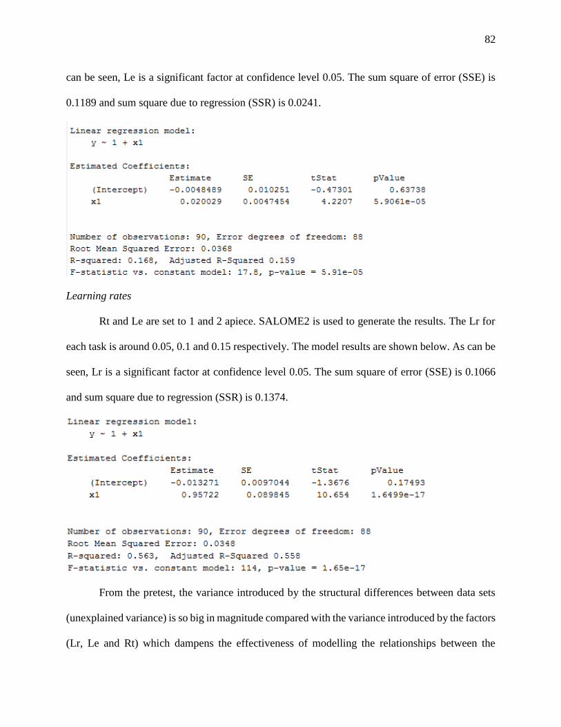
82
can be seen, Le is a significant factor at confidence level 0.05. The sum square of error (SSE) is
0.1189 and sum square due to regression (SSR) is 0.0241.
Learning rates
Rt and Le are set to 1 and 2 apiece. SALOME2 is used to generate the results. The Lr for
each task is around 0.05, 0.1 and 0.15 respectively. The model results are shown below. As can be
seen, Lr is a significant factor at confidence level 0.05. The sum square of error (SSE) is 0.1066
and sum square due to regression (SSR) is 0.1374.
From the pretest, the variance introduced by the structural differences between data sets
(unexplained variance) is so big in magnitude compared with the variance introduced by the factors
(Lr, Le and Rt) which dampens the effectiveness of modelling the relationships between the

83
response and multiple factors. Hence, the linear model shall not be adopted in the formal design
of experiment. Instead, the one sample pairwise t-test is chosen as we test the two algorithms on
the same instance for all problems and control the other 3 variables at different levels. Considering
the production and learning process, we assign 3 levels (low, medium and high) to Lr, Le and Rt.
Lr is chosen from [0.05, 0.1, 0.15], Le is chosen from [1, 2, 3] and Rt is chosen from [1, 5, 10].
4.3.3 One sample t test
We specify the null hypothesis and alternative hypothesis as follows.
H0: The difference in the percentage improvement in production time between the two
algorithms are the same
H1: The percentage improvement in production time of ENCORE is greater than the
percentage improvement of SALOME2.
We use the power of statistical test to determine the sample size. In order to collect the
information to infer the sample size, a preliminary experiment is conducted. 16 problem instances
are selected with Rt, z, Le and Lr equal to 5, 400, 3 and 0.05 respectively. The mean improvement
of SALOME2 is 0.0685 and the standard deviation is 0.039. The mean improvement of ENCORE
is 0.0889. Under one sample and one sided t test, we conclude that the sample size should be
greater than 25 when we require the power to be greater than 0.8 and confidence level to be 0.95.
Therefore, 25 out of 80 instances are randomly chosen as experimental units.
There are 27 separate t tests for all combinations of levels in Lr, Le and Rt. In each t test,
two algorithms are examined on 25 instances respectively. Hence, a total of 1350 (27×2×25) runs
are performed. We report the p value and summary statistics (mean, standard deviation and lower
bounds of the 95% confidence interval) in Tables 15 and 16. As can be seen from Table 15, with
Rt equal to 1 second, the mean percentage differences in response between ENCORE and

84
SALOME2 of almost all cases is above 1.5%. However, with Rt equal to 5 and 10 seconds, the
improvements are not very obvious for all cases. Furthermore, from Table 16, the p value in bold
means that the corresponding null hypothesis is rejected under confidence level 0.95. The null
hypothesis is rejected 15 out of 27 times. The computer codes used in these experiments are
documented in Appendix F.
Table 15 Summary statistics for each t test on response comparisons (Eq. 26)
Difference of
improvements
between
algorithms
Time limit (s)
1 5 10
N Lr Le M SE CI M SE CI M SE CI
400
0.05
1 0.0245 0.0087 0.0097 0.0076 0.0051 -0.0011 0.0083 0.0054 -0.0009
2 0.0298 0.0103 0.0122 0.0084 0.0054 -0.0010 0.0088 0.0058 -0.0011
3 0.0296 0.0095 0.0133 0.0119 0.0063 0.0011 0.0094 0.0059 -0.0006
0.1
1 0.0155 0.0060 0.0052 0.0045 0.0026 0.0000 0.0041 0.0028 -0.0008
2 0.0183 0.0063 0.0074 0.0084 0.0038 0.0019 0.0073 0.0038 0.0009
3 0.0179 0.0063 0.0071 0.0107 0.0044 0.0032 0.0107 0.0044 0.0031
0.15
1 0.0256 0.0092 0.0098 0.0061 0.0039 -0.0006 0.0031 0.0022 -0.0007
2 0.0247 0.0087 0.0098 0.0053 0.0037 -0.0009 0.0041 0.0032 -0.0013
3 0.0214 0.0073 0.0088 0.0065 0.0038 0.0000 0.0060 0.0036 -0.0002

85
Table 16 p value matrix for each t test
pvalue Time limit (s)
1 5 10
N Lr Le
400
0.05
1 0.0047 0.0733 0.0672
2 0.0040 0.0689 0.0703
3 0.0023 0.0352 0.0610
0.1
1 0.0083 0.0491 0.0808
2 0.0042 0.0189 0.0316
3 0.0047 0.0114 0.0120
0.15
1 0.0053 0.0669 0.0850
2 0.0045 0.0785 0.1008
3 0.0038 0.0502 0.0557
The pairwise experiments empirically show that ENCORE has an advantage over
SALOME2 in production statistics at low run time level. Practically speaking, low run time or near
real time response is desirable in automated systems. The SCADA node and computer network
may be controlling different assembly lines and production equipment simultaneously, and there
may not be much time allotted for each individual optimization process.
The boundary (improvement difference or Rt) at which the null hypothesis is rejected can
be explored by running several t test with different Rt while holding other parameters fixed. With
the collected data points of p values and mean of improvements, the boundary can be interpolated.
For instance, we choose z=400, Lr=0.1 and Le=1 for analysis. We run the experiment with Rt
chosen from {1, 1.5, 2, 2.5, 3, 4, 5, 7, 8, 10}. The boundary for the improvement difference is
0.45% and for Rt is 5.24 seconds. We show the relationship of p value against improvement
difference in Figure 24.

86
Figure 24 Relationship between p value and improvement (Spline interpolation is used to
find the boundary)
4.4 Summary
In this chapter we demonstrate the rebalancing of the assembly line during small production
run when the task time attribute is non-constant. A novel algorithm—ENCORE is proposed, in
order to address the typical SALBP2 with non-constant task time attributes. Computational studies
show that ENCORE clearly outperforms the conventional algorithm which iteratively solves the
problem, making it a better method for application in real time automated systems.
The implementation of the rebalancing schedule is tested for assembly line problems under
uncertain task time attribute. Pairwise t tests are conducted to show the significance of superiority
of ENCORE over SALOME2 empirically at various computational time limits, appropriate for
real time decisions in advanced automated systems.

87
5. Priority rules-based algorithmic design on two sided assembly line balancing
In this section, we develop a priority rules-based algorithmic design for optimizing a two-
sided assembly line. Five elementary rules, ninety composite rules are tested on benchmark data
sets and their performances are provided. Two enumerative principles which are specific to two-
sided assembly lines are proposed to enhance the performance of the rules. Statistical analysis is
provided to complement the studies. Further, priority rules are embedded into a bounded dynamic
programing framework to form a novel algorithm where the use of a bound can reduce the solution
space as the algorithm is advanced stage-by-stage. A new optimal solution is found and contributed
to the existing literature. Furthermore, with the task learning considered, the production statistics
generated by each rule are reported.
5.1 The investigation of PRBMs in TALBP
In this section, we examine the performance of 5 elementary rules on benchmark data sets
obtained from Khorasanian et al. (2013). Totally 34 problem instances are examined. Then, we
design task assignment principles which are TALBP specific to improve the performance of the
elementary rules. Statistical analysis is provided to compare the performance of the elementary
rule set, as well as the performance enhancements, before and after the principles are incorporated.
Five elementary rules are paired with each other with different weights to constitute 90 composite
rules which are examined on the benchmark data set as well. We denote Avg_dev, which is the
percentage average deviation of the results found by PRBMs from the current best results in
Khorasanian et al. (2013), as the performance measure for PRBMs.

88
5.1.1 Application of elementary rules
The elementary rules selected in this paper are maximum task time (T), maximum TdL,
maximum TdS, maximum F and minimum L. The rules are self-explanatory or can be calculated
from the Eq. (2) and (3) in section 1.4. Note, the calculations of the earliest (Eli) and latest (Lai)
possible position to which task i can be assigned are shown in Eqs. (28) and (29). The enumerative
procedure of elementary rules is depicted in the flow diagram (Figure 25). The assignable task is
defined as the task which conforms to all constraints. In order to increase the efficiency of finding
new assignable task sets, only the direct followers of the task just assigned to be added to the old
assignable task set would be considered. Then, the old assignable task set can be updated by
evaluating every task in the old set with regard to the cycle time constraints. When two assignable
tasks have the same priority scores, their natural orderings are used to break the order.
𝐸𝑙𝑖
{
⌈∑ 𝑡𝑟 + ∑ 𝑡 + ∈𝑃𝑟𝑒𝐿 ∑ 𝑡𝑒𝑒∈𝑃𝑟𝑒𝐸𝑟∈𝑃𝑟𝑒𝑅
2𝑐⌉ 𝑖𝑓 ∑ 𝑡𝑒
𝑒∈𝑃𝑟𝑒𝐸
> | ∑ 𝑡 − ∑ 𝑡𝑟𝑟∈𝑃𝑟𝑒𝑅 ∈𝑃𝑟𝑒𝐿
|
⌈max(∑ 𝑡𝑟𝑟∈𝑃𝑟𝑒𝑅 , ∑ 𝑡 ∈𝑃𝑟𝑒𝐿 )
𝑐 ⌉ 𝑂𝑡ℎ𝑒𝑟𝑤𝑖𝑠𝑒
(28)
𝑎𝑖
{
𝑈𝐵 + 1 − ⌈
∑ 𝑟 ∑ 𝑙 𝑙∈𝑆𝑢𝑐𝐿∑ 𝑒𝑒∈𝑆𝑢𝑐𝐸𝑟∈𝑆𝑢𝑐𝑅
2𝑐⌉ 𝑖𝑓 ∑ 𝑡𝑒𝑒∈𝑆𝑢𝑐𝐸 > |∑ 𝑡 − ∑ 𝑡𝑟𝑟∈𝑆𝑢𝑐𝑅 ∈𝑆𝑢𝑐𝐿 |
𝑈𝐵 + 1 − ⌈max(∑ 𝑟𝑟∈𝑆𝑢𝑐𝑅
,∑ 𝑙𝑙∈𝑆𝑢𝑐𝐿)
𝑐 ⌉ 𝑂𝑡ℎ𝑒𝑟𝑤𝑖𝑠𝑒
(29)
Where

89
SucR, SucL, SucE are the sets of task i‘s successors whose operational directions are right, left and
either respectively.
PreR, PreL, PreE are the sets of task i‘s predecessors whose operational directions are right, left
and either respectively.
Figure 25 The enumerative procedure of elementary PRBMs
In Table 17 we present the average performance of the 5 elementary rules, where
performance is defined as the average percent deviation from the best known solution. As can be
seen, maximum F, though not obvious, is demonstrated to be the best elementary rule. Paired t

90
tests comparing the Avg_dev are conducted and p values are provided in Table 18. In line with the
results in Table 17, among 10 paired comparisons, only the performance between rule F and L,
where the most discrepancies occur, shows significant difference statistically. Hence, almost no
rule has an obvious edge against others. Equivalently speaking, each rule has its own advantage.
The Matlab codes to implement the elementary rules are in Appendix G.
Table 17 Average performance of the elementary rules
Rule TDS TDL T L F
Avg_dev (%) 17.43 16.65 16.55 20.84 12.15
Table 18 p values of paired t tests of Avg_dev of elementary rules (95% confidence level)
TDS TDL T L F
TDS 1 0.828 0.9759 0.2465 0.2186
TDL 1 0.8028 0.3548 0.1585
T 1 0.2288 0.2232
L 1 0.0224
F 1
As previously stated, the amount of idle time is the determinant of the quality of solutions.
We notice that there is a great amount of idle time from delay relative to the idle time from
remaining capacity after analyzing the structure of the solutions reported by the elementary rules.
Further, we infer that the major cause for the delay is the mated station imbalance where the station
load from one mated station is always higher than the other during the enumerative process. A
simple example is shown in Figure 26.

91
Figure 26 Top: 4 task data set; Middle: Solution 1; Bottom: Solution 2
Two solutions are provided based on two different enumerative principles respectively,
which are prior to the PRBMs on determining the order of tasks in the assignable task set. The first
principle is to assign the task which will minimize delay after the task is assigned (delay-oriented).
The second principle is to assign the task to the mated-station whose load is smaller than the other
(load-oriented). At first glance, the first rule seems superior to the second one because of its direct
reduction in the amount of idle time. However, it shows contradictory results. According to the
first rule, tasks 1, 2 and 3 are assigned in succession to left station and no delay occurs. When it
comes to task 4, however, a new position has to be opened because there is no room for task 4 in
position 1. As for the second solution, task 2 is assigned to the right station after task 1 because
such action balances the load between mated-stations. 3 units of time is delayed in the right station.
Then task 3 is assigned to left station because the load of station 1 (3 units of time) is smaller than
that of right station (6 units of time). Finally, task 4 is assigned to the left station. Solution 2 results
in less delay overall and, ultimately, generates less NM than solution 1 does. Hence, we adopt the

92
second principle prior to the first one. In other words, the assignable task set is sorted by the load-
oriented, delay-oriented and the task priority score in succession. The combinatorial structure of
principles is implemented throughout later analysis.
Analogous to the previous analysis, we test the performance of PRBMs with the proposed
principles (PRBMs_Plus) as shown in Table. 19. As can be seen, the performance of every
elementary rule is improved. Moreover, it is of our interest to test the influence of the principles
on the performance of the PRBMs. Table. 20 shows the p value of the paired t-test of Avg_dev
before and after the principles are incorporated. As a result, the performance of rule TdS and TdL
is significantly improved respectively and the improvement for the T is marginal. As for rule L and
F, there is no significant difference statistically. The Matlab codes to implement the elementary
rules with two principles are in Appendix H.
Table 19 Average performance of the elementary rules with two principles
TdS_Plus TdL_Plus T_Plus L_Plus F_Plus
Avg_dev (%) 9.88 8.45 9.68 15.00 7.03
Table 20 p values of paired t tests of Avg_dev of elementary rules with and without two
principles (95% confidence level)
Plus
TdS 0.01608
TdL 0.03404
T 0.05262
L 0.1122
F 0.1491

93
5.1.2 Application of composite rules
We adopt the construction scheme of composite rules in Otto and Otto (2014). Every pair
of 5 elementary rules is linearly summed which results in 10 basic composite rules. For each
composite rule, two weights are given to the 2 elementary rule respectively. The first weight is
chosen from the set {100, 10, 5, 2, 1/2, 1/5, 1/10, 1/100}. The second weight is always equal to 1.
Those configurations give a total of 90 composite rules. The enumerative procedure of composite
rules is similar to that of the elementary rule. It should be noted that all rules should be scaled in
order to be combined on equal footing. The scaled factor is given in Table. 21. The formula to
calculate the priority score of task i given weight j is shown in Eq. (30).
𝑖_𝑐𝑜𝑚𝑝𝑗
𝑊𝑒𝑖𝑔ℎ𝑡 (𝑗) × 𝑖_𝑒 𝑒𝑚 𝑐𝑎𝑙𝑒 𝑓𝑎𝑐𝑡𝑜𝑟𝑖_𝑒 𝑒𝑚
+ 𝑖_𝑒 𝑒𝑚2
𝑐𝑎𝑙𝑒 𝑓𝑎𝑐𝑡𝑜𝑟𝑖_𝑒 𝑒𝑚2 (30)
Table 21 The scaled factor for the application of composite rules
Rule TdS TdL T L F
Scaled factor c for denominator and GUB for nominator c GUB n
In Table. 22, we report the results of the best weighted combination for each pairing of
rules. For the ease of representation and comparison, the performance of the elementary rule (Table
19) is stored on the diagonal in bold. From the table we see that in all cases composite rules
outperform the elementary rule, indicating the combination of different rules provides synergy in
solving the TALBP. The performance of each weighted pairing rule in terms of the number of
best solutions it generates out of all 34 cases is presented in Table 23. The best weighted pairing
rules are {TdS; F; 0.01} and {Tdl; F; 0.1}, both of which outputs the 30 best results out of 34
problem instances.

94
Table 22 Average performance of the best weighted combinations for each pairing of rules
TdS TdL T L F
TdS 9.88 8.43 8.01 6.81 4.55
TdL 8.45 7.03 5.98 4.64
T 9.68 5.56 4.55
L 15 4.74
F 7.03
Table 23 The number of best solutions of each weighted pairing rules out of 34 cases as
measured by Avg_dev
Weight
100 10 5 2 1 0.5 0.2 0.1 0.01
TdS_TdL 20 19 19 18 17 18 19 18 20
TdS_T 20 18 19 15 15 17 19 19 21
TdS_L 19 16 16 18 15 15 16 14 14
TdS_F 20 20 19 20 22 23 25 26 30
TdL_T 21 20 20 19 19 19 19 19 22
TdL_L 22 19 19 16 19 17 17 16 16
TdL_F 20 20 20 23 24 25 29 30 28
T_L 22 16 17 17 19 18 16 16 16
T_F 21 21 24 21 25 28 29 29 29
L_F 18 18 19 20 19 19 21 24 27
From Tables 17 and 19, we observe that the performance of rule F is superior to the other
rules. We also notice, from Table 22, that the performance of the other 4 elementary rules are
greatly improved when paired with rule F. Also, from Table 23, the performance of F-related rules
improves as the weight that the F component receives also increases. Such relations are shown in

95
the panel plots in Figure 27. The Matlab codes to implement the composite rules are in Appendix
I.
Figure 27 Number of best solutions of composite rules in relation to the weight of F
5.2 Algorithmic design with BDP
In this section, the PRBMs are embedded into a bounded dynamic programming (BDP)
aiming to further improve the solution quality of stand-alone PRBMs as well as proposing a design
procedure. The novel algorithm (PR_BDP), which is comprised of two main components,
enumeration of states and solution space reduction is tested on benchmark data sets in order to
compare its performance against the best composite rules.

96
5.2.1 Enumeration of states
The procedure of enumerating states (positions) is the building block of the BDP. PRBMs
are applied to develop the states (partial solutions) at each stage. States which return small idle
time are carried forward to develop states at the next stage. The basic idea to use the PRBMs in
BDP is to take advantage of several good PRBMs in-stage performance and combine them
between the stages. For instance, applying composite rule L_F will result the minimum idle time
for position 1 and a relatively high idle time for position 2. As for rule T_F, the results are just the
opposite. If we apply the two rules independently, we obtain two mediocre solutions. However, if
we apply L_F to position 1 and T_F to position 2, we may get a solution that results in the minimum
overall idle time. To apply the enumeration procedure effectively, several techniques are applied.
These techniques are:
The choices of PRBMs. Instead of choosing all possible rules, we only adopt a few excellent
rules to develop the states at each stage for the sake of computational efficiency. Totally, 4 rules
are selected. The {TdS; F; 0.01} and {TdL; F; 0.1} are selected according to Table 23. Moreover,
{L; F; 0.01} and {T; L; 0.01} are added to the set of rules because they can provide better solutions
than the first two rules for some problems.
Assignable task set management. The running time during the enumeration procedure and
the quality of a partial solution highly depend on the generation of the assignable task set and the
order of the task in the set respectively. The assignable task set is updated and ordered based on
the following rules.
1) For a data set, the natural number of a task appears after all of its predecessor’s natural
number.

97
2) After a task is assigned, its successors along with the rest of the tasks in the previous
assignable task set are inspected on the cycle time constraint to constitute the new
assignable task set, which largely reduces the effort of reexamining all remaining tasks
on all constraints.
3) Tasks in the assignable task set are ordered according to the load-oriented rule, delay-
oriented rule, one of the 4 selected PRBMs and their natural number in succession.
5.2.2 Solution space reduction approaches
The solution space shall be relaxed in order to allow for the resolution of a large sized
problem as the PR_BDP advances in stages and between stages. For example, consider a problem
that requires 10 positions to assign all tasks. The total number of task sequence without space
reduction is 410=1,048,576 which greatly undermines the efficiency of the algorithm. Three
approaches are developed to reduce the solution space. 1) Labeling dominance rule, 2) utilization
of bounds, 3) window size.
Labeling dominance method. The labeling scheme (Schrage and Baker, 1978) ensures each
partial solution gets a unique value by assigning different labels to tasks. The states, developed by
different PRBMs, with the same total number of labels are deleted as the algorithm advances to
the next stage. As a consequence, the solution space is reduced, so is the computational speed. It
is an in-state reduction approach.
Utilization of bounds. The comparisons between different bounds (GLB, GUB, LB, UB)
can be used to delete the partial solutions whose prospective outputs can be proven to be not
superior to the existing best output. The global upper bound (GLB) can be calculated by ignoring
the precedence and indivisible constraints prior to the optimization process (see Wu, 2008). The

98
lower bound (LB) for each partial solution is equal to the summation of the number of positions
already finished and the global lower bound (GLB) for the remaining positions to which the rest
of tasks are assigned. The upper bound (UB) for each partial solution is generated by assigning the
first assignable task to the station without enumerating all tasks in the assignable task set. After all
tasks are assigned, the UB is equal to NM. Such a station construction scheme is the fastest method
to find a feasible solution meaning that the computational cost for UB is negligible. GUB is the
minimum UB among all partial solutions. The following comparisons are conducted and the
solution space is reduced accordingly.
1) UB and GLB. If a UB of a partial solution is equal to GLB (UB=GLB), the PR_BDP is
terminated and the optimum is GLB.
2) LB and GUB. For a partial solution, if its LB is not smaller than GUB (LB≥GUB), the
partial solution is proved to be dominated and can be deleted from the solution space.
3) UB and GUB. For a partial solution, if its UB is smaller than GUB, GUB is set to UB.
4) UB, LB and GUB. For a partial solution, if its LB is equal to UB but is less than GUB
(LB=UB<GUB), the full solution which results in the UB is stored as the best current
optimal solution, and then the partial solution is deleted from the solution space.
Comparisons 1 and 3 are conducted within stages during the enumerative process.
Comparisons 2 and 4 are conducted between stages after each enumerative process is done. Note,
the algorithm is terminated as the solution space is empty and the current best optimal solution is
reported.
Window size w. Window size, as defined in section 2.3, restricts a fixed number of states
at each state. The states are sorted in a non-descending order regarding the sum of idle times of
the assigned stations. Then, the first w states are reserved to develop states at next stage.

99
These approaches are deployed in the following order. The Labeling dominance rule is
first used to enumerate a state. Secondly, the comparison 1 is conducted to determine whether the
global optimum is found and the algorithm can be terminated. Thirdly, the comparison 3 is
assessed to update the GUB. Then, the comparisons 2 and 4 are conducted to eliminate the
unnecessary states. Finally, if the number of states remaining is greater than w, it is downsized to
w.
5.2.3 The application of PR_BDP
We formally develop the PR_BDP in the flow diagram below (Figure 28). It is graph-
based, deterministic and multi-pass solution generating process. It focuses on exploring the states
of a stage by exploiting the solution relaxation techniques to reduce the computational effort.
Figure 28 Structure of PR_BDP

100
We apply the PR_BDP with w equal to 5, which is an appropriate number to serve the
purposes of maintaining the quality of states as well as computational efficiency. The Avg_dev is
1.11%, as shown in Table 24 which is much improved from the performance of the best elementary
and composite rules reported in section 3. In table 25, we present the optimum found by PR_BDP
compared with the best NM reported in the literature. We also provide the computational times for
each instance as a means to gauge the computational efficiency. The CPU time is much smaller
than the cycle time of each instance which makes the algorithm applicable when task learning and
rebalancing are considered. Furthermore, a new optimum (NM=8 for A65, c=326 in Khorasanian
et al. (2013)) is found and proved. The Matlab codes to implement the PR_BDP are in Appendix
J.
Table 24 Comparisons of performance between best PRBMs and PR_BDP
Rule Best elementary rule Best composite rules PR_BDP
Avg_dev (%) 12.15 4.55 1.11
Table 25 Comparisons between the best NM reported and best NM generated by PR_BDP
Data set c Best reported NM NM (PR_BDP)
Computational times
(secs)
A12 4 4 4 0.54
5 3 3 0.11
6 3 3 0.02
7 2 2 0.05
A16 15 4 4 0.17
18 3 3 0.02
20 3 3 0.03
22 2 2 0.03
A24 25 3 3 0.31
30 3 3 0.06
35 2 2 0.07
40 2 2 0.09
A65 326 9 8 16.59
381 7 7 10.36
435 6 6 14.83

101
490 6 6 1.53
544 5 5 1.42
A148 204 13 13 5.33
255 11 11 5.87
306 9 9 7.14
357 8 8 3.91
408 7 7 2.53
459 6 6 2.48
510 6 6 3.15
A205 1133 11 11 5.80
1322 9 10 13.32
1510 8 9 7.56
1699 7 8 5.92
1888 7 7 3.25
2077 6 6 4.04
2266 6 6 3.07
2454 5 5 4.25
2643 5 5 2.19
2832 5 5 0.59
Computational experiments confirm the effectiveness of incorporating PRBMs into BDP.
The PR_BDP takes advantage of the capability of different composite rules on solving different
problems. The parameters need to be specified are the choice of PRBMs and the associated
weights. There are no ubiquitous parameters for all problems in general indicating that the analysis
in section 3 has to be performed in order to obtain the parameters. However, they can be found in
a short period of time because the search for the performance of each composite rule is a single-
pass, forward process, i.e., no backtracking is involved and only the best solution NM and score S
are stored in memory for each rule. Furthermore, the PR_BDP is terminated before enumerating
even half of the number of states for most problems. Thereby the assignable task set generation
and task allocation process are cut in half relatively to the elementary and composite rules which

102
require the assignment of all tasks. Such success of computational efficiency is attributed to the
relaxation techniques. Finally, with regards to the computational efficiency, the PR_BDP can
output the best solutions in a fast manner that it is appealing to deploy the PR_BDP in practice. It
is also worth to mention that the computational times of meta-heuristics are also very competitive,
e.g. Simulated annealing can output any individual solution within 5 seconds (Khorasanian et al.
(2013)). However, the endeavors to tune the parameters for each problem instance, which are not
always published in the literature, are a lot more time-consuming for the implementation of meta-
heuristics (Hooker, 1995).
5.2.4 Design of Experiments
In this section, some experiments, which are similar to the one in section 4.3, are performed
to assess the merit of task reassignment under the regime of two sided assembly system when
learning is taking place and it is desirable to reconfigure the assembly line in real time during a
production run. Considering learning provides two advantages. For one thing, it generates more
data instances with which our algorithm can be further tested. For another, production statistics
can be enhanced during the production process if task learning is held accountable. Because it is a
type 1 balancing problem, we adopt two performance measures—Average improvement of unit
NM (Avg_NM) and Average improvement of unit idle time (Avg_I) to evaluate the production
statistics of one problem. Learning period (Le) and learning rates (Lr) are used as control variables
as they are in section 4.3 representing the degree of learning. Equations (31) and (32) show the
calculations of the two terms.
𝐴𝑣𝑔_𝑁𝑀 ∑ 𝑁𝑀𝑖×𝑃𝐼𝑖𝐿𝑒+1𝑖=1
𝑁 (31)
𝐴𝑣𝑔_𝐼 ∑ 𝐼𝑖×𝑃𝐼𝑖𝐿𝑒+1𝑖=1
𝑁 (32)

103
Where PIi is the interval of the production process in which the total positions of the line is
NMi.
Given z=400, Le is selected from [1, 2, 3] and Lr is selected from [0.05, 0.1, 0.15]. The
novel algorithm PR_BDP is selected to output the best NMi in each production interval PIi. All
benchmark data instances (34) are selected for analysis. The summary statistics for the percent
improvement in Avg_NM and Avg_I are given below in Table. 26 and 27. The design of
experiment are programmed in Matlab and the codes are in Appendix K.
Table 26 Summary statistics for percent reduction in Avg_NM of 34 basic data instances
Avg_NM
Production quantity
Learning
rate
# of task
learning M SE 95% CI
400
0.05
1 0.0207 0.0072 0.0081
2 0.0455 0.0081 0.0313
3 0.0673 0.0084 0.0526
0.1
1 0.0475 0.0076 0.0343
2 0.0904 0.0062 0.0797
3 0.1298 0.0064 0.1185
0.15
1 0.0738 0.0062 0.0629
2 0.1323 0.0068 0.1205
3 0.1787 0.0081 0.1645
Table 27 Summary statistics for percent reduction in Avg_I of 34 basic data instances
Avg_I
Production quantity
Learning
rate
# of task
learning M SE 95% CI
400
0.05
1 0.1412 0.0484 0.0567
2 0.2874 0.0451 0.2087
3 0.3858 0.0415 0.3135
0.1
1 0.3078 0.0447 0.2297
2 0.4842 0.0279 0.4355
3 0.5748 0.0231 0.5345
0.15
1 0.4397 0.0392 0.3713
2 0.5794 0.0234 0.5386
3 0.6379 0.0298 0.5858

104
From the Tables 27 and 28, we can infer that the mean of both performance measures
increase in the Le and Lr. This means that, when comparing PR_BDP without dynamic
reconfiguration of the line to changing the configuration of the line when learning takes place,
Table 26 gives the percent reduction in Avg_NM and Table 27 gives the percent reduction in
Avg_I. Unlike the cases in section 4.3, where no obvious pattern can be observed, the positivity
correlation between the performance measures and Le or Lr of the current experiment is due to the
implementation procedure of algorithms. In the experiment of section 4.3, as for the large sized
data sets, we set time limit to restrict the total computational time of algorithm implementation in
order to control the cost of experiment because ENCORE and SALOME are exact solution
procedures. As such, there are possibilities that some data instances with the same precedence
relation but lower task times can produce higher output (cycle time). However, PR_BDP is a
heuristics approach which does not require the time limit to manage the overall cost of experiment.
In other words, outputs (NM and Idle time) are always smaller for higher degree of learning. In
practice, because of the excellent computational efficiency as shown in Table 25, one can use the
PR_BDP as an online algorithm to reassign tasks and reduce the number of positions as task
learning progresses.
5.3 Summary
In this chapter, we test the effectiveness of several elementary rules on TALBP. Two
principles (delay-oriented and load-oriented) are proposed, compared and utilized to minimize the
idle time from delay, which is a major negative impact on the performance of PRBMs. The
combinations of elementary rules (composite rules) provide synergetic advantage regarding the
average quality of solutions. Rule F with higher weight is the best partner when combined with

105
other elementary rules on solving the TALBP. Ultimately, an algorithmic design procedure
including selecting and incorporating PRBMs into BDP is proposed (PR_BDP), which is a
deterministic and problem specific heuristic procedure. Several important techniques are provided
to reduce the solution space significantly as the PR_BDP progresses. With the presence of task
learning, the improvement of production statistics is gauged by comparing task reassignment by
PR_BDP with the cases of no reassignment. Additionally, average computational times on test
problems are a fraction of cycle times, making real time application possible.
The design of algorithms provides distinct advantage over the traditional exact solution
procedure and meta-heuristics. Compared with the exact solution procedure, the efficiency is
greatly improved as the solution space is largely reduced and the quality of the developing solution
is maintained intelligently. Compared with the meta-heuristics, it is a ''white box'', intuitive process
which exploits the problem specific knowledge, e.g., the structure of the line, delay, time and
precedence relationships. Furthermore, the optimization process is deterministic which guarantees
the reproducibility of the results.

106
6. Summary
The assembly rebalancing with non-constant task time attribute problem is introduced and
solved in this dissertation. The rising problem is motivated by task learning effect during the
production process along the assembly line, and is established in the context of automatic assembly
line system, where assembly lines are operated by robots. In such a system the task time
improvement is preserved by the supervisory controller that oversees the assembly line and the
learned skill (information) can be transferred to other agents (robots) on the line. The collaborative
learning and structure of the supervisory control enable the line to be rebalanced as task time
improvements are realized in such a way that the overall efficiency of the line is optimized.
A total of three problems, residing in one-sided or two-sided assembly line, are addressed
by three different algorithms, either exact or heuristics solution procedure. To efficiently
implement those algorithms and apply the optimal solutions generated by them to assembly lines,
two rebalancing frameworks are proposed; 1) a planning framework, which is suitable for the
situation where task time improvements can be well estimated by a learning curve. This framework
relies on offline algorithms to generate the optimal solution for every production cycle; 2) a real
time framework, which is designed for the situation where task learning is uncertain, employs
online algorithms to obtain the optimal solution in real time.
A backward induction algorithm is capable of solving the task reassignment problem
efficiently, in which task times are reduced through learning and learning is conserved when tasks
are reassigned amongst stations so that the number of stations required in each production cycle is
minimized. The advantage of using the backward induction algorithm, is to avoid repetitively using
the tradition algorithm, e.g., SALOME, to produce the optimal solution in every production cycle
and, therefore, the computational burden is alleviated. Computational experiments are conducted

107
to validate the superiority of the backward induction algorithm over the conventional algorithm.
Furthermore, we demonstrate the industrial application of optimal solutions to the automated
assembly line with collaborative learning and supervisory control. It shows that the assembly
system is better off in production statistics considering rebalancing in each production cycle.
ENCORE is an online algorithm designed for solving the rebalancing problem with
uncertain task learning attribute. It leverages SALOME2 by using a near optimal starting point and
utilizing a temporary upper bound instead of the local lower bound, such that the computational
efficiency is improved. Pairwise t tests are conducted on large sized data instances to show
whether ENCORE is superior to SALOME2 empirically at various computational time limits,
appropriate for real time decisions in advanced automated systems. We also show the boundary at
which ENCORE has no advantage over SALOME2 statistically.
PR_BDP is designed by hybridizing dynamic programming and the priority-based method.
It takes its inspiration from the fact that the two-sided line balancing problem can be divided into
several subproblems that can be solved more easily than the main problem computationally, in
such a way that dynamic programming can be employed. In each subproblems, a solution can be
quickly generated by PRBMs, which is based on tasks’ priority scores, load-oriented and delay-
oriented principles. By piecing solutions of the subproblems together, the solution for the main
problem can be found. PR_BDP provides distinct advantage over the traditional exact solution
procedure and meta-heuristics. Compared with the exact solution procedure, the efficiency is
greatly improved as the solution space is largely reduced and the quality of the developing solution
is maintained intelligently. Compared with the meta-heuristics, it is a ''white box'', intuitive process
which exploits the problem specific knowledge. Furthermore, the optimization process is
deterministic, which guarantees the reproducibility of the results.

108
The aforementioned three algorithms and their features and applications are summarized
in table 28.
Table 28 Summary of Algorithms
Algorithm Attribute Application Features
Backward
induction Exact
one-sided line (type 1),
planning model
Avoid repetitively invoking traditional
method
ENCORE Exact
one-sided line (type 2),
real-time model
Use a near optimal starting point and a
better upper bound to ease computational
burden
PR_BDP Heuristic
two-sided line (type 1),
real-time model
Utilize both PRBMs and DP to divide the
problem and produce fast and good
solution
With the fast and efficient algorithms proposed, learning effects can be considered during
the course of production runs in practical production and operation management. In different
production environments (one-sided or two-sided line) with different goals (type 1 or type 2),
decision making processes depend on the optimal solutions resulting from different algorithms.
Concretely, decision makers should answer the following questions sequentially, and optimal
assembly line design and production schedule will be developed automatically.
What is the product?
By answering this question, we can decide which assembly line is suitable for production,
one-sided or two sided. If the size of the product is very large and requires workers to access the
unit from both sides of the part, two-sided lines shall be selected.
What is the production quantity?

109
We would like to know whether the dynamic rebalancing is necessary during the
production. As suggested in section 1.3, rebalancing during production is only meaningful when
the batch size is small, in which case the optimal solution is changed frequently. Otherwise, one
can rebalance the line once after the task learning reaches the plateau.
What is the goal?
The goal of designing an efficiently balanced line determines the problem types. If high
production rate is to pursue, then it is a type 2 problem in which cycle time is minimized. If the
amount of production capacity is the priority, then it is a type 1 problem where the number of
stations/positions is minimized.
How does task time behave?
The task learning process can be continuous or discrete in time, certain or uncertain. If the
learning process is continuous and almost certain, as in the insertion example of Figure 2. We can
approximate the path of task learning by a learning curve and select the planning model to
implement the rebalancing schedule. If the timing at which task learning occurs and/or the degree
of task time improvement are both uncertain, and they cannot be accurately predicted as using a
learning curve, we resort to the real-time rebalancing schedule.
Is there any time constraint on rebalancing the line?
At times there may be a time limit allowed for the algorithm to compute the optimal
solution to ensure the continuity of the production. In a planning model, that is not a concern
because it uses an offline algorithm. However, in real-time model, it becomes a factor that should
be considered in the rebalancing schedule, especially for a complex, large sized problem. We have
identified the boundary at which ENCORE is indifferent to SALOME2 in terms of the quality of
solutions. Statistically speaking, SALOME2 would generate as good results (cycle time) as

110
ENCORE does if the time limit is beyond the boundary. Their difference in objective value will
converge as the time limit increases, because they both are exact solutions.
In conclusion, to our knowledge this is the first work that addresses the case for
dynamically reconfiguring an assembly line during production under conditions where there is
learning or task time improvement and the knowledge underlying the improvement is retained as
tasks are redistributed among agents. This provides the opportunity to optimize overall production
efficiencies while maintaining constraints of the number of stations or the cycle time of the line.
This is the first work to focus on algorithmic design for such cases and to demonstrate their value
in industrial applications. As research on the application of flexible assembly systems with
machine learning progresses, these methods will help support the efficient planning of the use of
resources by taking into consideration optimal deployment over a range of task time reductions.
The results of this research can be extended in future research. One open issue includes
the global allocation of resources as agents (robots) become available during line reconfiguration.
At any time, there are multiple product assemblies to be schedules that will require resources
during a day’s schedule. Batches of different products are moved in and out of production and
require resources. Traditionally a line would be dedicated to one product at a time, though mixed
product lines are possible. As improvements take place in the assembly of one product and
resources can be reallocated, for example in the configuration of Figure 14, it opens the question
of how a full day’s production can be scheduled so as to maximize resource utilization overall.
This is the question that will be addressed in future research.

111
References
Arcus, A. L. (1965). A computer method of sequencing operations for assembly lines.
International Journal of Production Research, 4(4), 259-277.
Angerer, S., Pooley,R. and Aylett, R. (2010). Self-reconfiguration of industrial mobile robots,
Proceeding of Fourth IEEE International Conference on Self-Adaptive and Self-Organizing
Systems (2010), 64 – 73.
Babiceanu, R. and Chen, F. (2006). Development and application of holonic manufacturing
systems: A survey, Journal of Intelligent manufacturing 17, 111 – 131.
Bartholdi, J. J. (1993). Balancing two-sided assembly lines: A case study. International Journal
of Production Research, 31(10), 2447–2461.
Battaia, O., and Dolgui,A. (2012).Reduction approaches for a generalized line balancing problem.
Computers&OperationsResearch39,2337–2345.
Battaïa, O., and Dolgui,A. (2013). A taxonomy of line balancing problems and their solution
approaches. International Journal of Production Economics,142(2), 259-277.
Bautista, J., and Pereira, J. (2009). A dynamic programming based heuristic for the assembly line
balancing problem. European Journal of Operational Research, 194(3), 787-794.
Baybars, I (1986). A survey of exact algorithms for the simple assembly line balancing
problem. Management science ,32.8 , 909-932.
Baykasoglu, A., and Dereli, T. (2008). Two-sided assembly line balancing using an ant-colony-
based heuristic. The International Journal of Advanced Manufacturing Technology, 36(5-6),
582-588.
Biskup, D. (1999). Single-machine scheduling with learning considerations. European Journal of
Operational Research, 115(1), 173-178.
Boucher, T.O. (1996) Computer Automation in Manufacturing. London: Chapman & Hall.
Boucher, T.O. (1987). Choice of assembly line design under task learning. International Journal
of Production Research ,25.4 , 513-524.
Boucher, T.O. and A. Yalcin (2006) Design of Industrial Information Systems. Amsterdam:
Elsevier, Academic Press.
Boucher, T., & Li, Y. (2015). Technical note: systematic bias in stochastic learning. International
Journal of Production Research, 1-12.

112
Boysen, N., Fliedner, M., & Scholl, A. (2007). A classification of assembly line balancing
problems. European Journal of Operational Research, 183(2), 674-693.
Boysen, N., Scholl, A., &Wopperer, N. (2012). Resequencing of mixed-model assembly lines:
Survey and research agenda. European Journal of Operational Research, 216(3), 594-604.
Bryton, B. (1954). Balancing of a Continuous Production Line, M.S. Thesis, Northwestern
University, Evanston, IL
Bukchin, J., & Rubinovitz, J. (2003). A weighted approach for assembly line design with station
paralleling and equipment selection. IIE transactions,35(1), 73-85.
Bukchin, Y., &Rabinowitch, I. (2006). A branch-and-bound based solution approach for the
mixed-model assembly line-balancing problem for minimizing stations and task duplication
costs. European Journal of Operational Research,174(1), 492-508.
Cakir, B., Altiparmak, F., and Dengiz, B. (2011). Multi-objective optimization of a stochastic
assembly line balancing: A hybrid simulated annealing algorithm. Computers& Industrial
Engineering, 60(3), 376-384.
Cavalcante, A., Peixoto,J and Pereira.C. (2012). When agents meet manufacturing: paradigms and
implementations, Anais do XIX CongressoBrasileiro de Automatica, 957 – 964.
Coffman, Jr, E. G., Garey, M. R., & Johnson, D. S. (1978). An application of bin-packing to
multiprocessor scheduling. SIAM Journal on Computing, 7(1), 1-17.
Cohen, Y., Dar-El, M. (1998) Optimizing the number of stations in assembly lines under learning
for limited production, Production Planning and Control, 9 (3), 230–240.
Cohen, Y., Vitner, G., & Sarin, S. C. (2006). Optimal allocation of work in assembly lines for lots
with homogenous learning. European Journal of Operational Research, 168(3), 922-931.
Cohen, Y., Vitner, G., & Sarin, S. (2008) Work allocation to stations with varying learning slopes
and without buffers. European Journal of Operational Research, 184(2), 797-801.
Digiesi, S., Kock, A., Mummolo, G., Rooda, J. (2009). The effect of dynamic worker behavior on
flow line performance. International Journal of Production Economics, 120 (2), 368–377.
Dar-El, E. M. (1975). Solving large single-model assembly line balancing problems—A
comparative study. AIIE Transactions, 7(3), 302-310.
Dar-El, E.M., Rubinovitch, Y. (1979). MUST––A multiple solutions technique for balancing
single model assembly lines. Management Science 25, 1105–1114.
Dolgui, A., Finel, B., Vernadat, F., Guschinsky, N., & Levin, G. (2005). A heuristic approach for
transfer lines balancing. Journal of Intelligent Manufacturing, 16(2), 159-172.

113
Dolgui, A., Proth, J., (2010). Supply Chain Engineering: useful methods and techniques. Springer.
Easton, F., Faaland, B., Klastorin, T.D., Schmitt, T., (1989). Improved network based algorithms
for the assembly line balancing problem. International Journal of Production Research, 27, 1901–
1915.
Fleszar, K., & Hindi, K. S. (2003). An enumerative heuristic and reduction methods for the
assembly line balancing problem. European Journal of Operational Research, 145(3), 606-620.
Globerson, S., & Gold, D. (1997). Statistical attributes of the power learning curve
model. International journal of production research, 35(3), 699-711.
Goldberg, M. S., & Touw, A. (2003). Statistical methods for learning curves and cost analysis (p.
196). Institute for Operations Research and the Management Sciences (INFORMS).
Gurevsky, E., Hazır, Ö., Battaïa, O., &Dolgui, A. (2012). Robust balancing of straight assembly
lines with interval task times [star]. Journal of the Operational Research Society, 64(11), 1607-
1613.
Hackman, S.T., Magazine, M.J., Wee, T.S. (1989). Fast, effective algorithms for simple assembly
line balancing problems. Operations Research 37, 916–924.
Haupt, R. (1989): A survey of priority rule-based scheduling. OR Spectrum, 11, 3–16.
Held, M., Karp, R. M., &Shareshian, R. (1963). Assembly-line balancing-dynamic programming
with precedence constraints. Operations Research,11(3), 442-459.
Heskiaoff, H. (1968). A heuristic method for balancing assembly line. The western electric
engineering ,12/3,9-13
Hoffmann, T.R., (1963). Assembly line balancing with a precedence matrix. Management Science,
9, 551–562
Hoffmann, T.R. (1992). EUREKA: A hybrid system for assembly line balancing. Management
Science, 38.1, 39-47.
Hooker, J. N. (1995). Testing heuristics: We have it all wrong. Journal of heuristics, 1(1), 33-42.
Hu, X., Wu, E., & Jin, Y. (2008). A station-oriented enumerative algorithm for two-sided assembly
line balancing. European Journal of Operational Research, 186(1), 435-440.
Hu, X., Wu, E., Bao, J., & Jin, Y. (2010) A branch-and-bound algorithm to minimize the line
length of a two-sided assembly line. European Journal of Operational Research, 206(3), 703–707

114
Jackson, J. R. (1956). A computing procedure for a line balancing problem. Management
Science, 2.3 , 261-271.
Johnson, Roger V. (1988), Optimally balancing large assembly lines with "FABLE", Management
Science, 34.2 , 240-253.
Klein, R., Scholl, A. (1996). Maximizing the production rate in simple assembly line balancing––
A branch and bound procedure. European Journal of Operational Research 91, 367–385.
Khorasanian, D., Hejazi, S. R., & Moslehi, G. (2013). Two-sided assembly line balancing
considering the relationships between tasks. Computers & Industrial Engineering, 66(4), 1096-
1105.
Kim, Y. K., Kim, Y., & Kim, Y. J. (2000). Two-sided assembly line balancing: a genetic algorithm
approach. Production Planning & Control, 11(1), 44-53.
Lapierre, S. D., Ruiz, A., & Soriano, P. (2006). Balancing assembly lines with tabu
search. European Journal of Operational Research, 168(3), 826-837.
Lapierre, S. D., & Ruiz, A. B. (2004). Balancing assembly lines: an industrial casestudy. Journal
of the Operational Research Society, 589-597.
Lee, T. O., Kim, Y., & Kim, Y. K. (2001). Two-sided assembly line balancing to maximize work
relatedness and slackness. Computers & Industrial Engineering, 40(3), 273-292.
Li, Y., & Boucher, T. O. (2016). Assembly line balancing problem with task learning and dynamic
task reassignment. The International Journal of Advanced Manufacturing Technology, 1-9.
Lopes, L. S., &Camarinha-Matos, L. M. (1995).A machine learning approach to error detection
and recovery in assembly. IEEE International Conference on Human Robot Interaction and
Cooperative Robots ,3,197-203.
McNaughton, R., 1959. Scheduling with deadlines and loss functions. Management Science 6, 1–
12.
Mansoor, E.M. (1964), Assembly line balancing-an improvement on the ranked positional weight
technique. Journal of Industrial Engineering ,15.2 , 73-77.
Mastor, A. A. (1970), An experimental investigation and comparative evaluation of production
line balancing techniques. Management Science ,16.11, 728-746.
Miltenburg, J. (2001). U-shaped production lines: A review of theory and practice. International
Journal of Production Economics, 70(3), 201-214.

115
Nearchou, A. C. (2011). Maximizing production rate and workload smoothing in assembly lines
using particle swarm optimization. International Journal of Production Economics, 129(2), 242-
250.
Newnan, D.G., J.P. Lavelle, and T.G. Eschenbach (2009) Engineering Economic Analysis, (10th
ed.). New York: Oxford University press.
Nuttin, M. and van Brussel.H. (1999). Learning sensor assisted assembly operations, Making
Robots Smarter, K. Morik, M. Kaiser and V. Klingspor, eds. Kluwer Academic Publishers, 45 –
52.
Onori, M., Barata, J. and Frei, R. (2006). Evolvable assembly systems: basic principles,
Information Technology for Balanced Manufacturing Systems, International Feceration for
Information Processing, 220, 317-328
Ostwald, P.F. (1992) Engineering Cost Estimating, 3rd. Ed. Englewood Cliffs: Prentice Hall.
Otto, A., Otto, C., & Scholl, A. (2011). How to design and analyze priority rules: Example of
simple assembly line balancing. Working Papers in Supply Chain Management 3, Friedrich-
Schiller-University of Jena.
Otto, A., & Otto, C. (2014). How to design effective priority rules: Example of simple assembly
line balancing. Computers & Industrial Engineering, 69, 43-52.
Otto, C., and Otto, A. (2014). Extending assembly line balancing problem by incorporating
learning effects. International Journal of Production Research, 52(24), 7193-7208.
Özbakır, L., & Tapkan, P. (2010). Balancing fuzzy multi-objective two-sided assembly lines via
Bees Algorithm. Journal of Intelligent & Fuzzy Systems,21(5), 317-329.
Posypkin, M. A.E and Sigal, I. K. (2006). Speedup estimates for some variants of the parallel
implementations of the branch-and-bound method. Computational Mathematics and
Mathematical Physics ,46.12, 2187-2202.
Ribeiro, L., Barata, J. and Colombo, A. (2008). MAS and SOA: A case study exploring principles
and technologies to support self-properties in assembly systems, Proceedings of Second IEEE
Conference on Self-Adaptive and Self-Organizing Systems, 192-197.
Rekiek, B., Dolgui, A., Delchambre, A., and Bratcu, A. (2002). State of art of optimization
methods for assembly line design. Annual Reviews in Control,26(2), 163-174.
Rubinovitz, J., and Levitin, G. (1995). Genetic algorithm for assembly line balancing.
International Journal of Production Economics, 41(1), 343-354.
Sanders, D. and Gegovm, A. (2013) AI tools for use in assembly automation and some examples
of recent applications, Assembly Automation, 33 (2), 184-194.

116
Salveson, M.E. (1955). The assembly line balancing problem. Journal of Industrial
Engineering, 6.3, 18-25.
Scholl,A.(1993), data of assembly line balancing problem,
http://alb.mansci.de/index.php?content=classview&content=classview&content2=classview&co
ntent3=classviewdlfree&content4=classview&classID=44&type=dl
Scholl, A., & Voß, S. (1997). Simple assembly line balancing—Heuristic approaches. Journal of
Heuristics, 2(3), 217-244.
Scholl, A, and Klein, R. (1997). SALOME: A bidirectional branch-and-bound procedure for
assembly line balancing. INFORMS Journal on Computing, 9.4 ,319-334.
Scholl, A., & Klein, R. (1999). ULINO: Optimally balancing U-shaped JIT assembly
lines. International Journal of Production Research, 37(4), 721-736.
Scholl, A, and Klein, R. (1999). Balancing assembly lines effectively–a computational comparison,
European Journal of Operational Research, 114.1, 50-58.
Scholl, A and Becker, C. (2006). State-of-the-art exact and heuristic solution procedures for simple
assembly line balancing. European Journal of Operational Research ,168.3 ,666-693.
Schrage, L., & Baker, K. R. (1978). Dynamic programming solution of sequencing problems with
precedence constraints. Operations research, 26(3), 444-449.
Simaria, A. S., & Vilarinho, P. M. (2009). 2-ANTBAL: An ant colony optimisation algorithm for
balancing two-sided assembly lines. Computers & Industrial Engineering, 56(2), 489-506.
Sotskov, Y. N., Dolgui, A., Lai, T. C., & Zatsiupa, A. (2015) Enumerations and stability analysis
of feasible and optimal line balances for simple assembly lines. Computers & Industrial
Engineering, 90, 241-258.
Storer, R. H., Wu, S. D., & Vaccari, R. (1992). New search spaces for sequencing problems with
application to job shop scheduling. Management science, 38(10), 1495-1509.
Sullivan, W.G., E.M. Wicks, and C.P. Koelling (2015) Engineering Economy, 16th Ed. Upper
Saddle River: Pearson Prentice Hall.
Süer, G. A. (1998). Designing parallel assembly lines. Computers & industrial engineering, 35(3),
467-470.
Suresh, G., and Sahu, S. (1994). Stochastic assembly line balancing using simulated
annealing. The International Journal of Production Research, 32(8), 1801-1810.

117
Talbot, F. B., Patterson, J. H., & Gehrlein, W. V. (1986). A comparative evaluation of heuristic
line balancing techniques. Management science,32(4), 430-454.
Toksarı, M. D., İşleyen, S. K., Güner, E., and Baykoç, Ö. F. (2008). Simple and U-type assembly
line balancing problems with a learning effect. Applied Mathematical Modeling, 32(12), 2954-
2961.
Terwiesch, C., and Bohn, R. E. (2001). Learning and process improvement during production
ramp-up. International Journal of Production Economics ,70.1, 1-19.
Tuncel, G., & Aydin, D. (2014). Two-sided assembly line balancing using teaching–learning based
optimization algorithm. Computers & Industrial Engineering, 74, 291-299.
Ueda, K. (2007). Emergent synthesis approaches to biological manufacturing systems, Digital
Enterprise Technology, Springer, 25 – 34.
Van Hop, N. (2006). A heuristic solution for fuzzy mixed-model line balancing
problem. European Journal of Operational Research, 168(3), 798-810.
Vance, P. H., Barnhart, C., Johnson, E. L., & Nemhauser, G. L. (1994). Solving binary cutting
stock problems by column generation and branch-and-bound. Computational optimization and
applications, 3(2), 111-130.
Vigil, D. P., & Sarper, H. (1994). Estimating the effects of parameter variability on learning curve
model predictions. International journal of production economics, 34(2), 187-200.
Wang, B., Guan, Z., Li, D., Zhang, C., & Chen, L. (2014). Two-sided assembly line balancing
with operator number and task constraints: a hybrid imperialist competitive algorithm. The
International Journal of Advanced Manufacturing Technology, 74(5-8), 791-805.
Whitney, D.E. (1982). Quasi-static assembly of compliantly supported rigid parts. Transactions of
ASME, Journal of Dynamic Systems Measurement and Control, 104 (1), 65-77.
Wu, E. F., Jin, Y., Bao, J. S., & Hu, X. F. (2008). A branch-and-bound algorithm for two-sided
assembly line balancing. The International Journal of Advanced Manufacturing
Technology, 39(9-10), 1009-1015.
Yelle, L. E. (1979). The learning curve: Historical review and comprehensive survey. Decision
Sciences, 10(2), 302-328.
Yuan, B., Zhang, C., & Shao, X. (2015). A late acceptance hill-climbing algorithm for balancing
two-sided assembly lines with multiple constraints. Journal of Intelligent Manufacturing, 26(1),
159-168.
Zacharia, P. T., & Nearchou, A. C. (2012). Multi-objective fuzzy assembly line balancing using
genetic algorithms. Journal of Intelligent Manufacturing,23(3), 615-627.

118
Appendix A: Benchmark data sets
Small sized data set are displayed in their precedence graph. Big sized data set in a table
consisting two parts, task times (the first column) and direct precedence relations (the second
column)
Figure 29 Precedence graph of Mansoor's data set
Figure 30 Precedence graph of Heskiaoff's data set

119
Large sized data sets
Kilbrid Arcus (83) Arcus (111) Bartholdi Scholl
45 1,3 83 1,2 111 1,2 148 1,5 297 1,2
9 1,7 1673 2,3 1960 2,3 16 1,6 270 2,3
9 2,4 985 2,4 1715 3,4 30 1,7 270 3,4
10 2,8 1836 2,5 735 4,5 7 1,8 130 4,5
10 3,5 973 3,6 1715 4,6 47 2,3 148 4,22
17 4,6 1700 4,6 490 4,7 29 3,4 190 4,26
17 5,9 2881 4,7 1225 4,8 8 3,5 293 4,27
13 6,10 2231 5,8 169 4,9 39 3,6 348 4,40
13 7,9 1040 6,9 2252 4,10 37 3,7 182 4,48
20 7,14 1793 6,10 1225 5,39 32 4,8 490 4,56
20 8,10 1250 7,11 2319 6,39 29 5,14 212 4,83
10 8,14 700 8,77 1715 7,83 17 6,9 248 4,86
11 9,41 464 8,78 980 8,71 11 7,14 248 4,94
6 10,41 500 9,12 735 9,32 32 8,10 248 4,105
22 11,13 1133 10,13 2281 10,11 15 9,14 248 4,109
11 12,13 577 10,14 2750 10,12 53 10,14 248 4,111
19 12,37 483 10,25 77 11,13 53 11,12 268 4,134
12 13,14 880 11,15 89 11,14 8 12,13 268 4,221
3 13,15 667 12,16 51 11,15 24 14,15 268 4,247
7 14,17 600 13,17 364 11,16 24 14,16 288 4,259
4 14,25 233 13,18 405 11,17 8 15,17 248 5,6
55 14,29 408 13,20 3060 11,18 7 16,17 268 6,7
14 14,30 847 14,19 125 11,19 8 17,18 60 6,8
27 14,31 767 15,20 3429 11,20 14 17,19 268 6,9
29 14,32 850 15,39 43 11,21 13 18,20 240 6,10
26 15,16 780 16,77 3430 12,13 10 19,20 240 7,11
6 15,18 912 16,78 1960 12,14 25 20,21 171 7,12
5 15,23 748 17,21 29 12,15 11 20,22 490 7,13
24 15,24 1863 17,22 27 12,16 25 20,23 182 7,14
4 16,19 714 17,28 15 12,17 11 20,24 170 7,15
5 17,26 1004 18,23 121 12,18 29 21,25 306 7,20
7 17,27 713 19,24 1715 12,19 25 21,26 108 8,11
4 18,19 642 20,26 2127 12,20 10 21,27 248 8,12
15 19,20 629 21,27 1470 12,21 14 21,28 190 8,13
3 19,33 1234 22,27 4037 13,71 41 22,25 240 8,14
7 20,21 1143 23,74 68 14,22 42 22,26 339 8,15
9 21,22 1266 24,28 62 14,23 47 22,27 288 8,20
4 22,28 792 24,29 42 14,24 7 22,28 248 9,11
7 23,33 1251 25,32 364 14,25 80 23,25 455 9,12
5 24,33 1310 26,74 4998 15,26 7 23,26 268 9,13
4 25,26 663 27,69 1470 16,27 41 23,27 270 9,14

120
21 26,38 494 28,32 2963 17,28 47 23,28 180 9,15
12 27,28 1288 29,30 5689 18,29 16 24,25 121 9,20
6 27,33 792 30,31 68 19,30 32 24,26 270 10,11
5 28,38 578 31,39 18 20,91 66 24,27 440 10,12
5 29,41 594 32,33 10 21,111 80 24,28 249 10,13
30,41 578 32,34 81 22,31 7 25,29 194 10,14
31,41 622 32,35 5200 22,83 41 26,29 162 10,15
32,41 578 32,36 39 23,32 13 27,29 130 10,20
33,34 564 33,37 67 23,33 47 28,29 388 11,16
33,35 578 34,77 27 24,69 33 29,31 90 12,17
33,36 578 34,78 15 24,70 34 31,36 212 13,18
34,38 578 35,77 121 25,34 11 32,34 246 14,19
35,40 578 35,78 58 26,82 18 33,35 188 15,21
36,38 578 36,38 1715 27,35 25 34,36 270 16,23
37,43 578 36,39 125 28,36 7 35,36 160 17,23
38,40 578 37,40 4010 29,37 28 36,37 79 18,23
39,41 578 38,41 1470 30,38 12 37,38 466 19,23
40,41 578 39,42 1470 31,39 52 37,45 240 20,23
41,42 578 39,43 2303 32,41 14 38,39 137 21,23
42,44 578 39,44 1960 33,111 3 39,40 184 22,24
42,45 578 39,75 2205 34,42 3 40,41 110 22,25
578 40,77 4018 35,43 8 40,48 275 23,28
578 40,78 2744 36,44 16 40,54 149 24,29
578 41,45 2999 36,91 33 42,43 280 25,29
578 42,77 735 37,45 8 43,44 119 26,30
578 42,78 735 37,91 18 45,46 184 27,31
578 43,77 735 38,46 10 46,47 140 28,32
578 43,78 735 38,91 14 47,48 150 28,37
467 44,46 545 39,40 28 47,49 190 29,33
887 45,47 3386 40,111 11 47,54 150 29,44
396 46,48 3234 41,69 18 50,51 150 29,121
1296 47,49 2205 41,70 25 51,53 284 30,34
1100 48,50 2206 42,47 40 51,69 192 30,297
2543 49,69 490 43,48 40 52,53 347 31,34
764 50,51 825 43,49 1 54,55 232 31,82
357 51,52 3528 44,50 5 54,72 140 31,172
701 52,53 3568 45,51 28 54,76 608 31,179
1164 53,54 1200 46,52 8 54,89 80 32,36
286 54,55 618 47,54 81 54,90 40 33,38
2100 55,56 1470 47,55 7 55,133 130 34,35
450 56,57 1715 47,56 26 56,73 110 35,42
1300 57,58 735 47,57 10 57,82 350 36,39
3691 58,59 1960 47,58 21 58,86 140 37,39

121
59,60 2889 47,59 26 58,88 240 38,41
60,61 618 47,60 20 59,75 240 39,43
61,62 490 48,53 21 59,89 90 40,44
62,63 735 49,91 47 61,62 54 40,84
63,64 490 50,111 23 62,63 294 40,97
64,65 921 51,111 13 63,67 203 41,45
65,66 326 52,111 19 64,65 150 42,46
66,67 5390 53,111 15 64,71 270 43,47
67,68 243 54,69 35 64,72 155 44,49
68,74 371 54,70 26 65,66 190 45,50
68,75 58 55,61 46 65,99 78 46,51
69,70 5059 55,62 20 66,67 140 46,138
69,71 1225 55,63 31 67,68 241 47,52
70,72 769 56,63 19 68,95 430 48,52
71,73 768 56,64 34 68,98 90 49,53
72,73 1670 57,65 51 69,79 110 50,54
73,74 1670 57,91 39 70,71 9 51,55
73,75 490 58,66 30 72,134 430 51,81
74,76 202 58,91 26 73,86 130 52,57
75,76 203 59,67 13 73,88 289 53,58
76,77 202 59,91 45 73,89 110 54,58
76,78 2744 60,68 58 73,90 160 54,296
77,79 162 60,91 28 73,96 442 55,59
78,79 324 61,69 8 74,75 159 56,60
79,80 162 61,70 83 75,90 250 56,61
79,81 121 62,71 40 75,97 190 57,62
80,82 162 63,111 34 76,77 184 57,63
81,83 91 64,72 23 77,78 690 57,71
82,83 65,111 62 78,82 72 57,76
66,111 11 79,85 190 58,64
67,111 19 79,80 190 59,64
68,111 14 79,143 90 59,99
69,77 31 79,146 889 59,100
69,78 32 80,81 170 60,68
70,73 26 81,82 155 61,65
71,91 55 82,83 190 62,66
72,74 31 83,84 130 63,67
73,75 32 84,106 390 64,72
74,76 26 86,87 301 65,69
75,77 19 90,111 54 66,69
75,78 14 91,105 227 67,70
75,79 19 92,135 142 68,73
76,80 48 95,101 184 69,74

122
76,81 55 96,104 741 70,75
76,82 8 98,101 868 71,77
77,83 11 99,100 230 72,78
78,84 27 100,101 121 73,84
79,85 18 101,102 320 73,97
80,86 36 101,103 126 74,84
80,91 23 102,127 440 74,97
81,87 20 103,127 127 75,84
81,91 46 105,119 134 75,97
82,111 64 106,107 150 76,84
83,91 22 107,108 140 76,97
84,88 15 108,109 110 77,84
84,89 34 109,110 320 77,97
84,91 22 111,112 250 78,79
85,111 51 112,113 232 78,80
86,111 48 113,114 188 78,125
87,90 64 113,116 250 78,192
88,105 70 113,120 377 79,85
89,105 37 113,123 90 80,85
90,111 64 113,128 140 81,87
91,92 78 114,115 90 82,88
91,93 78 115,125 90 82,89
91,94 116,117 70 83,90
92,95 117,118 90 84,91
93,95 118,126 110 85,92
94,95 120,121 150 86,93
95,96 121,122 101 87,99
95,97 122,126 377 87,100
95,98 123,124 118 88,99
95,99 124,125 290 88,100
95,100 128,129 209 89,99
95,104 129,130 150 89,100
96,101 130,131 150 90,95
97,102 130,137 79 91,96
98,103 132,135 150 92,98
99,111 133,135 91 93,98
100,111 134,135 59 94,101
101,105 135,136 218 95,101
102,106 138,139 351 96,101
102,107 139,140 873 97,101
103,107 141,142 130 98,102
103,108 142,143 68 99,103
104,111 142,146 126 100,104

123
105,111 142,147 120 101,106
106,109 142,148 227 102,107
107,111 144,145 198 103,108
108,110 145,147 132 104,108
109,111 145,148 121 105,110
110,111 150 106,112
100 107,113
38 108,114
70 108,115
355 108,292
284 109,119
122 109,120
75 110,119
160 110,120
140 110,162
520 111,116
99 112,117
182 113,118
80 114,119
514 115,120
96 116,122
50 117,123
272 117,124
226 117,257
194 118,126
164 119,127
96 120,127
107 120,150
108 121,128
167 122,129
98 123,130
82 123,145
482 123,146
72 123,147
50 123,148
130 123,149
230 124,130
50 125,130
240 126,130
190 127,130
190 127,157
240 128,130
74 129,130

124
139 129,141
339 130,131
260 130,144
132 131,132
550 131,133
420 132,135
152 133,135
12 133,170
90 134,136
5 135,137
128 136,139
100 137,140
120 138,140
100 138,191
320 139,142
835 139,253
740 140,143
223 140,200
100 141,151
390 142,152
140 143,153
304 143,169
120 144,154
403 145,155
21 146,156
246 147,158
160 148,159
1019 149,160
34 150,161
120 151,163
68 152,164
910 153,165
302 154,166
778 155,166
101 156,166
1310 157,166
20 158,166
278 159,166
81 160,166
290 161,166
100 162,167
372 163,166
72 164,167

125
28 165,168
90 165,176
250 166,170
144 167,171
303 168,173
220 169,174
58 170,174
224 171,174
211 172,175
99 173,177
44 174,178
120 174,287
70 174,288
421 175,180
231 176,181
214 177,181
196 178,181
280 179,181
398 180,181
72 180,252
280 181,182
356 181,183
193 181,184
140 181,185
130 181,186
300 181,187
456 181,188
7 181,189
170 181,196
252 181,197
210 181,295
308 182,190
308 183,193
121 184,194
52 185,195
426 186,195
104 187,195
1386 188,195
527 189,195
968 190,195
1047 191,200
538 192,201
193,198

126
194,199
195,199
195,203
195,205
195,227
195,229
196,202
197,202
198,202
199,202
200,202
201,202
202,204
202,251
203,206
203,208
204,207
204,250
205,207
206,209
207,210
207,212
208,210
209,210
209,211
210,213
211,213
212,214
213,214
214,215
214,234
215,216
216,217
217,218
218,219
219,220
220,222
221,223
222,224
223,225
224,226
225,227
226,228

127
227,230
228,231
229,235
229,236
230,232
230,271
230,289
231,233
232,236
233,237
234,238
234,256
235,237
236,239
237,240
238,240
238,285
239,240
239,279
240,241
240,243
241,242
242,244
243,245
243,246
244,245
244,246
244,255
245,248
246,248
247,278
248,249
249,254
249,284
250,256
251,256
252,258
253,260
254,261
255,261
255,262
256,263
257,264

128
258,265
259,266
260,267
261,268
261,269
262,269
263,270
264,271
265,272
266,271
267,273
268,274
269,274
270,274
271,274
272,275
273,276
274,277
274,278
274,282
275,280
276,281
277,283
278,283
279,286
280,290
281,291
282,293
283,293
284,294
285,294
286,294
287,293
288,293
289,294
290,293
291,293
292,293
A65 (Lee et al., 2001), E stands for either side, R and L stand for right and left side respectively.
Task Side
Task
time Immediate successors
1 E 49 3

129
2 E 49 3
3 E 71 4,23
4 E 26 5,6,7,9,11,12,25,26,27,41,45,49
5 E 42 14
6 E 30 14
7 R 167 8
8 R 91 14
9 L 52 10
10 L 153 14
11 E 68 14
12 E 52 14
13 E 135 14
14 E 54 15,18,20,22
15 E 57 16
16 L 151 17
17 L 39 31
18 R 194 19
19 R 35 21
20 E 119 21
21 E 34 31
22 E 38 31
23 E 104 24
24 E 84 31
25 L 113 31
26 R 72 31
27 R 62 28
28 R 272 50
29 L 89 50
30 L 49 50
31 E 11 32,36,51,52,53,54,55,56,58,59,60,61,62
32 E 45 33
33 E 54 34
34 E 106 35
35 R 132 50
36 E 52 37
37 E 157 38
38 E 109 39,40
39 L 32 50
40 R 32 50
41 E 52 42
42 E 193 43
43 E 34 62
44 R 34 46
45 L 97 46
46 E 37 47

130
47 L 25 48
48 L 89 50
49 E 27 50
50 E 50 66
51 R 46 65
52 E 46 65
53 L 55 65
54 E 118 65
55 R 47 65
56 E 164 57
57 E 113 65
58 L 69 65
59 R 30 65
60 E 25 65
61 R 106 65
62 E 23 63
63 L 118 64
64 L 155 65
65 E 65 -
New optimal solution. For each position, the first row indicates the mated station to which the
task is assigned, 1 is the left station and 2 is the right station; the second row are the task sequences.
Position 1
1 2 1 2 1 1 2 1 1 2 2 1
1 2 3 13 4 9 11 12 5 6 44 49
Position 2
1 2 1 1 2 2
23 7 41 10 8 27
Position 3
1 2 1 2 1 2 1
14 24 20 18 25 19 22
Position 4
1 2 1 2 2 1 1 1 2
15 26 16 21 42 17 31 36 60
Position 5
1 2 1 1 2 1 2 1 2 2
32 37 43 45 33 46 62 38 51 52
Position 6
1 2 1 2 1 1 2
34 56 63 35 47 58 59
Position 7
2 1 1 1 2 1
28 48 64 30 55 39

131
Position 8
1 2 1 2 1 2 2 1
57 54 29 61 53 40 50 65

132
Appendix B: The basic flow chart of ENCORE

133
Appendix C: Computational tests for backward induction algorithm
Matlab codes for computational test in section 3.4.1&3.4.2
Tables 5–10 are generated by SALOME and backward induction algorithm.
The steps of execution are as follows.
1) Open the test script
2) Adjust the parameters (learning rate, data set, batch size)
3) Run the script
Sample test script (Backward induction algorithm (weak) )
clear all
tic
learning=0.95;
alpha=log(learning)/log(2);
c=168;
n=30;
load Heskiaoff
[OS,Sq,m,Tsq,avg_dev,omitted_B]= Algo1_weak(c,P,t0,n,learning);
elapsed_time=toc;
Sample test script (Backward induction algorithm (strong) )
clear all
tic
learning=0.95;
alpha=log(learning)/log(2);
c=168;
n=30;
load Heskiaoff
[OS,Sq,m,Tsq,avg_dev,omitted_B]= Algo1_strong(c,P,t0,n,learning);
elapsed_time=toc;
Sample test script (SALOME)
clear all
tic;
learning=0.9;
alpha=log(learning)/log(2);
c=168;
n=10;
total_dev=[];
omitted_B=0;
Tsq=0;
load Heskiaoff

134
for i=1:n-1
t(:,i)=t0.*i^alpha;
end
t(:,n)=t0.*n^alpha;
answer=[];
for i=1:n
[OS,Sq,m,UM]=mainSALOME(c,P,t(:,i));
Tsq=Tsq+size(Sq,1);
total_dev=[total_dev;(UM-min(UM))/(min(UM)-1)*100];
answer=[answer,m];
end
av_dev=mean(total_dev);
elapsed_time=toc;
The main function for SALOME:
function [OS,Sq,m,UM]=mainSALOME(c,P,t)
%Jackson dominance rule
%find all followers&direct followers
D_Mat=Jackson_Dominance(P,t);
[S,Sq,UM,LM,cs,Idle]=FinFea(c,P,t);
b=ones(length(t),1);
d=Sq;
Lt=length(d);
OS=S;
GLM=ceil(sum(t)/c)+1;
if UM==GLM
m=UM;
else
%whether or not the SALOME is finished
Fin=0;
while 1
[S,b,cs,d,Lt,Idle,Fin]=Backtrack(S,b,cs,d,Lt,t,c,LM,Idle,Fin);
if Fin==1
break
end
%set the uniqueness equal to zero
Uni=0;
while 1
%store states for later retrieval
b1=b;
S1=S;

135
d1=d;
d2=[];
[S,Sq,b,d,Lt,LM,cs,Idle,Uni,d2]=StationLoadsFinder(S,Sq,b,d,cs,L
M,UM,Lt,Idle,Uni,c,P,t,d2,D_Mat);
if Uni==0
b=b1;
S=S1;
d=d1;
end
if Uni==1
break
end
[S,b,cs,d,Lt,LM,Idle,Fin]=Backtrack1(S,b,cs,d,LM,t,c,Idle,Fin);
if Fin==1
break
end
end
if Fin==1
break
end
[OS,S,Sq,b,d,cs,Lt,LM,UM,Idle]=NewSeqGen(OS,S,Sq,b,d,cs,LM,UM,Lt
,Idle,c,P,t,D_Mat);
if UM==GLM
break
end
end
m=UM;
end
end
The main function for backward induction algorithm (weak):
function [OS,Sq,m,Tsq,avg_dev,omitted_B]=
Algo1_weak(c,P,t0,n,learning)
%calculate the task time of all repetitions.
alpha=log(learning)/log(2);
omitted_B=0;
for i=1:n
t(:,i)=t0.*i^alpha;
end
%Initialize the Optimal solution set
OS=zeros(length(t0),length(t0),n);

136
m=zeros(1,n);
%find the first optimal solution
total_dev=[];
[OS(:,:,n),Sq,m(n),UM]=mainSALOME(c,P,t(:,n));
total_dev=[total_dev;(UM-min(UM))/(min(UM)-1)*100];
Tsq=size(Sq,1);
%start the explosion theory
i=n;
while 1
D=OS(:,:,i)*t0;
e=max(D);
j=floor((c/e)^(1/alpha));
if i-j>=2
%in this case, the deviation to optimality is zero
total_dev=[total_dev;zeros(i-j-1,1)];
%total BnB skipped
omitted_B=omitted_B+i-j-1;
m(j+1:i-1)=m(i);
for k=j+1:i-1
OS(:,:,k)=OS(:,:,i);
end
end
if j==0;
break
end
i=j;
[OS(:,:,i),Sq,m(i),UM]=mainSALOME(c,P,t(:,i));
total_dev=[total_dev;(UM-min(UM))/(min(UM)-1)*100];
Tsq=Tsq+size(Sq,1);
if i==1
break
end
end
avg_dev=mean(total_dev);
end
The main function for backward induction algorithm (strong):
function [OS,Sq,m,Tsq,omitted_B]= Algo1_strong(c,P,t,n)
%Initialize the Optimal solution set
OS=zeros(size(t,1),size(t,1),n);
m=zeros(1,n);
%find the first optimal solution

137
[OS(:,:,n),Sq,m(n),UM]=mainSALOME(c,P,t(:,n));
Tsq=size(Sq,1);
omitted_B=0;
%start the explosion theroy
for i=n-1:-1:1
%initialize the feasibiliy=1
fea=1;
OS(:,:,i)=OS(:,:,i+1);
m(i)=m(i+1);
for j=1:m(i)
if OS(j,:,i)*t(:,i)>c
fea=0;
break
end
end
if fea==1
OS(:,:,i)=OS(:,:,i+1);
m(i)=m(i+1);
omitted_B=omitted_B+1;
else
[OS(:,:,i),Sq,m(i),UM]=mainSALOME(c,P,t(:,i));
Tsq=Tsq+size(Sq,1);
end
end
end
The sub-functions called by the SALOME or backward induction algorithm are presented as
follows.
The function of finding a feasible solution
function [S,Sq,UM,LM,cs,Idle]=FinFea(c,P,t)
%find the lm for station 1 which is loaded by the first node
LM(1)=ceil(sum(t)/c)+1;
%find the available idle time
Idle=(LM(1)-1)*c-sum(t);
%b is the array storing all of the assigned tasks
b=[1;zeros(length(t)-1,1)];

138
%initialize station¤t station put a dummy task(0) into a
fake station
S=zeros(length(t),length(t));
S(1,1)=1;
cs=2;
%initialize assignable task&sequence
at=[];
Sq=[1 0];
%begin the loop
while 1
%find the assignable task
for i=2:length(t)
%%three requirements:1 task has not been assigned 2 its
predecessors
%%have been assigned 3 it could not exceed its cycle time
if b(i)~=1 && b'*P(:,i)==sum(P(:,i)) && c-S(cs,:)*t-t(i)>=0
%i-1 is actually the task number!
at=[at,i];
end
end
%assign task
%check if there is any room to assign any task
if isempty(at)
%calculate the remaining idle time(definition: the remaining
idle time
%of the station is calculated in absence of any assignment to
that station)
Idle=Idle-(c-S(cs,:)*t);
if Idle>=0
LM(cs)=LM(cs-1);
else
LM(cs)=LM(cs-1)+1;
%one more station time to spare!
Idle=Idle+c;
end
cs=cs+1;
Sq=[Sq 0];
else
%find max task time to assign
[a,index]=max(t(at(1:end)));
%retrieve the index of the task
index=at(index);
S(cs,index)=1;
Sq=[Sq,index];
b(index)=1;
end

139
if b==ones(length(t),1)
break
end
% reset assignable task array
at=[];
end
%put an artificial LM for root node, the last LM is the current UM
LM=[LM(1),LM];
%find the current m which is the upper bound of the optimal
solution
for i=1:length(t)
if sum(S(i,:))==0
UM=i-1;
break
end
end
end
Backtrack function
function[S,b,cs,d,Lt,Idle,Fin]=Backtrack(S,b,cs,d,Lt,t,c,LM,Idle
,Fin)
%station oriented backtrack
%backtrack process follows the new sequence
%find the last station whose LM is smaller than current station's
LM
k=find(LM==LM(cs)-1,1,'last');
%backtrack to k
if isempty(k)
%current solution is the optimal solution
Fin=1;
else
%empty the stations and sequences from k to current station
Index2=find(d==0,k-1);
d(Index2(end):end)=0;
%release the idle time of the station
Idle=Idle+((cs-k)*c-sum(S(k:(cs-1),:)*t));
for j=k:cs
Index1= S(j,:)~=0;
b(Index1)=0;
S(j,:)=0;
end

140
%reduce one full station time
Idle=Idle-c;
cs=k;
%set the last task: find the (k-1)th zero in the current
sequence, the last task is next to it.
E=find(d==0,k-1);
Lt=E(end)+1;
end
end
Station enumeration function
function
[S,Sq,b,d,Lt,LM,cs,Idle,Uni,d2]=StationLoadsFinder(S,Sq,b,d,cs,L
M,UM,Lt,Idle,Uni,c,P,t,d2,D_Mat)
at=[];
for i=find(b==0,1):length(t)
if b(i)~=1&&b'*P(:,i)==sum(P(:,i)) && c-S(cs,:)*t-t(i)>=0
at=[at,i];
end
end
%downsize the assignable task by Jackson's dominance rule
if length(at)>=2
Dominated_task=[];
for o=1:length(at)
for r=(o+1):length(at)
%is at(o) dominating at(r)?
if ismember(at(r),D_Mat(at(o),:))
Dominated_task=[Dominated_task;r];
elseif ismember(at(o),D_Mat(at(r),:))
%is at(r) dominating at(o)?
Dominated_task=[Dominated_task;o];
end
end
end
at(Dominated_task)=[];
end
if isempty(at)
OL=[];
for k=1:size(Sq,1)
if isequal(Sq(k,1:Lt-1),d(1:Lt-1))
OL=1;
break
end
end

141
%if the new load is of the same local lower bound or branched
before,
%give it up.
%TLM:temporary local lower bound
if Idle-(c-S(cs,:)*t)>=0
TLM=LM(cs);
else
TLM=LM(cs)+1;
end
if ~isempty(OL)||TLM>LM(cs+1)|| TLM>=UM
%give it up, empty the current task in the current station
and sequence(revert to the last state )
Lt=Lt-1;
b(d(Lt))=0;
S(cs,d(Lt))=0;
d(Lt)=0;
else
%calculate the local lower bound
LM(cs+1)=TLM;
Uni=1;
Idle=Idle-(c-S(cs,:)*t);
if LM(cs+1)>LM(cs)
Idle=Idle+c;
end
cs=cs+1;
E=find(d==0,cs-1);
Lt=E(end)+1;
end
else
for j=1:length(at)
b(at(j))=1;
d(Lt)=at(j);
S(cs,at(j))=1;
Lt=Lt+1;
[S,Sq,b,d,Lt,LM,cs,Idle,Uni,d2]=StationLoadsFinder(S,Sq,b,d,cs,L
M,UM,Lt,Idle,Uni,c,P,t,d2,D_Mat);
if Uni==1
%already find an unique solution, stop permuting
break
end
% if j is the last choice, but it is still not working,
erase the previous selection when previous selection exists.
if j==length(at)&&d(Lt-1)~=0
Lt=Lt-1;
b(d(Lt))=0;
S(cs,d(Lt))=0;

142
d(Lt)=0;
end
end
end
end
Superior solution generation function
function
[OS,S,Sq,b,d,cs,Lt,LM,UM,Idle]=NewSeqGen(OS,S,Sq,b,d,cs,LM,UM,Lt
,Idle,c,P,t,D_Mat)
%station oriented BB
at=[];
while 1
%find the assignable task
for i=2:length(t)
%%three requirements:1 task has not been assigned 2 its
predecessors
%%have been assigned 3 it could not exceed its cycle time
if b(i)~=1 && b'*P(:,i)==sum(P(:,i)) && c-S(cs,:)*t-t(i)>=0
%i-1 is actually the task number!
at=[at,i];
end
if length(at)>=2
Dominated_task=[];
for o=1:length(at)
for r=(o+1):length(at)
%is at(o) dominating at(r)?
if ismember(at(r),D_Mat(at(o),:))
Dominated_task=[Dominated_task;r];
elseif ismember(at(o),D_Mat(at(r),:))
%is at(r) dominating at(o)?
Dominated_task=[Dominated_task;o];
end
end
end
at(Dominated_task)=[];
end
end
%assign task
%check if there is any room to assign any task
if isempty(at)
%calculate the remaining idle time(definition: the remaining
idle time
%of the station is calculated in absence of any assignment to
that station)
Idle=Idle-(c-S(cs,:)*t);

143
if Idle>=0
LM(cs+1)=LM(cs);
else
LM(cs+1:end)=LM(cs)+1;
%one more station time to spare!
Idle=Idle+c;
end
%Compare the local LM and the global UM
if LM(cs+1)>=UM
%done! stop generating the sequence, backtrack
Sq=[Sq;d];
size(Sq,1)
cs=cs+1;
break
else
cs=cs+1;
d(Lt)=0;
Lt=Lt+1;
end
else
%find max task time to assign
[a,index]=max(t(at(1:end)));
%retrieve the index of the task
index=at(index);
S(cs,index)=1;
d(Lt)=index;
b(index)=1;
Lt=Lt+1;
end
if b==ones(length(t),1)
Sq=[Sq;d];
Idle=Idle-(c-S(cs,:)*t);
%New UM
UM=LM(cs);
LM(cs+1)=LM(cs);
cs=cs+1;
OS=S;
break
end
% reset assignable task array
at=[];
end
end

144
Appendix D: Case study
Matlab codes for the case study in section 3.5
Table 11 is generated by the following script.
t0=[6;6;5;5;4;5;4;2;9;2];
learning=0.85;
c=10;
n=30;
t=zeros(10,n);
P =[
0 1 1 1 1 1 1 1 1 1 1
0 0 1 0 0 1 0 0 0 0 0
0 0 0 0 0 0 0 1 0 0 0
0 0 0 0 1 0 0 0 0 0 0
0 0 0 0 0 1 0 0 0 0 0
0 0 0 0 0 0 1 0 0 0 0
0 0 0 0 0 0 0 0 1 0 0
0 0 0 0 0 0 0 0 1 0 0
0 0 0 0 0 0 0 0 0 1 0
0 0 0 0 0 0 0 0 0 0 1
0 0 0 0 0 0 0 0 0 0
0];
alpha=log(learning)/log(2);
for i=1:n
t(:,i)=t0.*i^alpha;
end
%without rebalancing %({3,4},{1,5},{2,7}, {6,8},{9} {10}) .
TI_wo=0;
for i=1:30
T1(1)=c-(t(3,i)+t(4,i));
T1(2)=c-(t(1,i)+t(5,i));
T1(3)=c-(t(2,i)+t(7,i));
T1(4)=c-(t(6,i)+t(8,i));
T1(5)=c-t(9,i);
T1(6)=c-t(10,i);
TI_wo=TI_wo+sum(T1);
end
%with rebalacning unit 1 %({3,4},{1,5},{2,7}, {6,8},{9} {10})
T1=[];
TI_w=0;
T1(1)=c-(t(3,1)+t(4,1));
T1(2)=c-(t(1,1)+t(5,1));
T1(3)=c-(t(2,1)+t(7,1));
T1(4)=c-(t(6,1)+t(8,1));
T1(5)=c-t(9,1);

145
T1(6)=c-t(10,1);
TI_w=TI_w+sum(T1);
T1=[];
%unit 2,3, ({1,3},{2,4},{5,6},{7,8},{9,10}
for i=2:3
T1(1)=c-(t(1,i)+t(3,i));
T1(2)=c-(t(2,i)+t(4,i));
T1(3)=c-(t(5,i)+t(6,i));
T1(4)=c-(t(7,i)+t(8,i));
T1(5)=c-t(9,i)-t(10,i);
TI_w=TI_w+sum(T1);
end
T1=[];
%unit 4-9, ({1,3},{2,4},{5,6,7},{8,9,10}).
for i=4:9
T1(1)=c-(t(1,i)+t(3,i));
T1(2)=c-(t(2,i)+t(4,i));
T1(3)=c-(t(5,i)+t(6,i)+t(7,i));
T1(4)=c-(t(8,i)+t(9,i)+t(10,i));
TI_w=TI_w+sum(T1);
end
T1=[];
%unit 10-30, ({1,3,4},{2,5,6},{7,8,9,10}).
for i=10:30
T1(1)=c-(t(1,i)+t(3,i)+t(4,i));
T1(2)=c-(t(2,i)+t(5,i)+t(6,i));
T1(3)=c-(t(7,i)+t(8,i)+t(9,i)+t(10,i));
TI_w=TI_w+sum(T1);
end
TS_rebal=1*6+2*5+6*4+21*3

146
Appendix E: Computational tests for ENCORE
Matlab codes for computational test in section 4.2.5
Tables 12–14 are generated by SALOME2 and ENCORE.
The steps of execution are as follows.
1) Open the test script
2) Adjust the parameters (data set, batch size)
3) Run the script
Sample test function (ENCORE)
clear all;
m=8;
load Arcus83
%generate random task time matrix
n=30;
t1=zeros(length(t),n);
Q=t;
for i=1:n
for j=2:length(t)
t1(j,i)=ceil(Q(j)-random('uni',0.8,1)*t(j)*0.02);
end
Q=t1(:,i);
end
tic
[OptiC1,Sq1,OS1]=MainSALOME2(m,P,t);
Tsq3=0;
Tsq=0;
TB=0;
aa=1;
for i=1:n
[OptiC,Sq1,OS1,B]=Algorithm3(Sq1,OS1,m,P,t1(:,i));
Tsq3=Tsq3+size(Sq1,1);
TB=TB+B;
aa=aa+1
end
a=toc;
bb=0;
Tsq=0;
%optimum is not found in current solution
UNF=0;
for i=1:n
[OptiC,Sq,OS]=MainSALOME2(m,P,t1(:,i));

147
if size(Sq,1)>=1000
UNF=UNF+1;
end
Tsq=Tsq+size(Sq,1);
bb=bb+1
end
b=toc;
c=b-a;
Main function for SALOME2
function [OptiC,Sq,OS]=MainSALOME2(D_Mat,m,P,t,ct)
%ct computational time requirement
[S,Sq,UB,LM,TOI,TOIL]=FinFea(m,P,t);
if UB==max(ceil(sum(t)/m),max(t))
OptiC=UB;
OS=S;
else
%backtrack
OS=S;
d=Sq;
Lt=length(d);
b=ones(length(t),1);
cs=m+1;
Fin=0;
%start recording computational time
tic;
while 1
%%enter the first backtrack
[S,d,cs,Lt,b,TOI,TOIL,Fin]=Backtrack(S,b,cs,d,Lt,t,m,LM,TOI,TOIL
,Fin);
if Fin==1
break
end
%set the uniqueness equal to zero
Uni=0;
while 1
[S,b,d,Lt,LM,cs,TOI,TOIL,Uni]=StationLoadsFinder(S,Sq,b,d,cs,LM,
UB,Lt,TOI,TOIL,Uni,m,P,t,D_Mat);
if Uni==1
break

148
end
while 1
%enter the second backtrack(one station per time)
[S,d,cs,Lt,b,TOI,TOIL,Fin]=Backtrack1(S,b,cs,d,Lt,t,m,LM,TOI,TOI
L,Fin);
if Fin==1
break
end
[S,b,d,Lt,LM,cs,TOI,TOIL,Uni]=StationLoadsFinder(S,Sq,b,d,cs,LM,
UB,Lt,TOI,TOIL,Uni,m,P,t,D_Mat);
if Uni==1
break
end
end
if Uni==1
break
end
if Fin==1
break
end
end
if Fin==1
break
end
[OS,S,Sq,b,d,cs,Lt,LM,UB,TOI,TOIL,Fin]=NewSeqGen(OS,S,Sq,b,d,cs,
LM,UB,Lt,TOI,TOIL,m,P,t,D_Mat);
TOC=toc;
%exit the problem when toc>ct
if TOC>ct
OptiC=UB;
break
end
end
end
OptiC=UB;
end
The function of finding a feasible solution
function [S,Sq,UB,LM,TOI,TOIL]=FinFea(m,P,t)
%Starting from a lower bound
LB=ceil(sum(t)/m);

149
%find the lm for station 1 which is loaded by the first node
LM(1)=ceil(sum(t)/m);
TOI=m*LB-sum(t);
TOIL(1)=TOI;
%b is the array storing all of the assigned tasks
b=[1;zeros(length(t)-1,1)];
at=[];
at1=[];
%current station
cs=2;
%initialize station¤t station put a dummy task(0) into a
fake station
S=zeros(length(t),length(t));
S(1,1)=1;
Sq=[1 0];
while 1
for i=2:length(t)
%%three requirements:1 task has not been assigned 2 its
predecessors
%%have been assigned 3 it could not exceed its cycle time
if b(i)~=1 && b'*P(:,i)==sum(P(:,i)) && LB-S(cs,:)*t-
t(i)>=0
%i-1 is actually the task number!
at=[at,i];
end
end
if isempty(at)
%calculate the total idle time left
if TOIL(cs-1)-(LB-S(cs,:)*t)<0
%find the lowest available task to assign
for i=2:length(t)
%%two requirements:1 task has not been assigned 2
its
predecessors %%have been assigned
if b(i)~=1 && b'*P(:,i)==sum(P(:,i))
%i-1 is actually the task number!
at1=[at1,i];
end
end
[a,index1]=min(t(at1(1:end)));
%retrieve the index of the task
index1=at1(index1);
S(cs,index1)=1;
Sq=[Sq,index1];
b(index1)=1;

150
%increase the local lower bound
LM(cs)=S(cs,:)*t;
LB=LM(cs);
%update the TOI&TOIL
TOI=m*LM(cs)-sum(t);
tempTOIL=TOI;
for j=2:cs
tempTOIL=tempTOIL-(LB-S(j,:)*t);
end
TOIL(cs)=tempTOIL;
at1=[];
else
TOIL(cs)=TOIL(cs-1)-(LB-S(cs,:)*t);
LM(cs)=LM(cs-1);
end
cs=cs+1;
Sq=[Sq 0];
else
%find max task time to assign
[a,index]=max(t(at(1:end)));
%retrieve the index of the task
index=at(index);
S(cs,index)=1;
Sq=[Sq,index];
b(index)=1;
end
if b==ones(length(t),1)
%at times, there may be one or more station vacant when
the
%assignment is done!
if cs==m+1
TOIL(cs)=TOIL(cs-1)-(LB-S(cs,:)*t);
LM(cs)=LM(cs-1);
break
else
%take out the last tasks from the last station and fill
them the into to the vacant station.
for k=1:(m+1-cs)
cc(k)=Sq(end-k+1);
Sq(end-k+1)=0;
end
S(cs,cc(1:end))=0;
cc=fliplr(cc);
l=length(cc);
for k=1:length(cc)
Sq(end-l+2)=cc(k);

151
Sq(end-l+3)=0;
l=l-1;
TOIL(cs)=TOIL(cs-1)-(LB-S(cs,:)*t);
LM(cs)=LM(cs-1);
cs=cs+1;
S(cs,cc(k))=1;
TOIL(cs)=TOIL(cs-1)-(LB-S(cs,:)*t);
LM(cs)=LM(cs-1);
end
Sq(length(t)+m+1:end)=[];
break
end
end
% reset assignable task array
at=[];
end
UB=LM(end);
end
Backtrack function (SALOME2)
function
[S,d,cs,Lt,b,TOI,TOIL,Fin]=Backtrack(S,b,cs,d,Lt,t,m,LM,TOI,TOIL
,Fin)
%station oriented backtrack
%backtrack process follows the new sequence
aa=sum(t);
%find the last station whose LM is Equal to current station's
LM,empty it
%out
k=find(LM==LM(cs),1);
if k==1 || cs==1
%current solution is the optimal solution
Fin=1;
else
%empty the stations and sequences from k to current station
Index2=find(d==0,k-1);
d(Index2(end):end)=0;
%recalculate the TOI and TOIL
TOI=LM(k-1)*m-aa;
TOIL(1)=TOI;
for j=2:(k-1)
TOIL(j)=TOIL(j-1)-(LM(k-1)-S(j,:)*t);

152
end
for j=k:cs
Index1= S(j,:)~=0;
b(Index1)=0;
S(j,:)=0;
end
cs=k;
%set the last task:find the (k-1)th zero in the current
sequence, the last task
%is next to it.
E=find(d==0,k-1);
Lt=E(end)+1;
end
end
Station enumeration function (SALOME2)
function
[S,b,d,Lt,LM,cs,TOI,TOIL,Uni]=StationLoadsFinder(S,Sq,b,d,cs,LM,
UB,Lt,TOI,TOIL,Uni,m,P,t,D_Mat)
%%ONLY ONE chance of keep on going to generate new sequence 1)the
%%lower bound is not increasing at next station
at=[];
at1=[];
if d(Lt-1)==0
for i=find(b==0,1):length(t)
if b(i)~=1&&b'*P(:,i)==sum(P(:,i)) && UB-S(cs,:)*t-t(i)>0
at=[at,i];
end
end
else
for i=d(Lt-1)+1:length(t)
if b(i)~=1&&b'*P(:,i)==sum(P(:,i)) && UB-S(cs,:)*t-t(i)>0
at=[at,i];
end
end
end
%%downsize the assignable task by Jackson's dominance rule
if length(at)>=2
Dominated_task=[];
for o=1:length(at)
for r=(o+1):length(at)
%is at(o) dominating at(r)?
if ismember(at(r),D_Mat(at(o),:))
Dominated_task=[Dominated_task;r];
elseif ismember(at(o),D_Mat(at(r),:))

153
%is at(r) dominating at(o)?
Dominated_task=[Dominated_task;o];
end
end
end
at(Dominated_task)=[];
end
if isempty(at)
%check the overlapping first 1) if overlap, forfeit the
solution 2)if
%not, check the feasibility by TOIL
%if the station is empty now, consider increase
OL=[];
for k=1:size(Sq,1)
if isequal(Sq(k,1:Lt),d(1:Lt))
OL=1;
break
end
end
%if the new load is of the same local lower bound or
branched before,
%give it up.
if isempty(OL)
AA=max(LM(cs-1),S(cs,:)*t);
%check whether the TOIL is less than zero
tempTOIL=AA*m-sum(t);
for j=2:cs
tempTOIL=tempTOIL-(AA-S(j,:)*t);
if tempTOIL<0
break
end
end
if tempTOIL>=0
%the solution is good
LM(cs)=AA;
Uni=1;
TOI=m*LM(cs)-sum(t);
tempTOIL=TOI;
for j=2:cs
tempTOIL=tempTOIL-(LM(cs)-S(j,:)*t);
end
TOIL(cs)=tempTOIL;
cs=cs+1;
E=find(d==0,cs-1);
Lt=E(end)+1;
else

154
%forfeit the solution
Lt=Lt-1;
b(d(Lt))=0;
S(cs,d(Lt))=0;
d(Lt)=0;
end
else
%forfeit the solution
Lt=Lt-1;
b(d(Lt))=0;
S(cs,d(Lt))=0;
d(Lt)=0;
end
else
for j=1:length(at)
b(at(j))=1;
d(Lt)=at(j);
S(cs,at(j))=1;
Lt=Lt+1;
[S,b,d,Lt,LM,cs,TOI,TOIL,Uni]=StationLoadsFinder(S,Sq,b,d,cs,LM,
UB,Lt,TOI,TOIL,Uni,m,P,t,D_Mat);
if Uni==1
%already find an unique solution, stop permuting
break
end
% if j is the last and only choice , but it is still not
working, erase the previous selection(j) when previous selection
exists(has not been erased in the ifempty(at) part).
if j==length(at)&&d(Lt-1)~=0
Lt=Lt-1;
b(d(Lt))=0;
S(cs,d(Lt))=0;
d(Lt)=0;
end
end
end
end
Superior solution generation function (SALOME2)
function
[OS,S,Sq,b,d,cs,Lt,LM,UB,TOI,TOIL,Fin]=NewSeqGen(OS,S,Sq,b,d,cs,
LM,UB,Lt,TOI,TOIL,m,P,t,D_Mat)
%station oriented BB

155
at=[];
at1=[];
Fin=0;
while 1
%if there is no task left, but it has not reached the last station
%relocate last few tasks to last few stations and recalculate the
UB
if sum(b)==length(t)&&cs<=m
%the station is full, but cs did not increase by i, which it
should
cs=cs+1;
k=m+2-cs;
%withdraw the tasks
v=find(d~=0,1,'last');
aa=d(v-k+1:v);
%set the S(v) to zero
for o=1:length(aa)
S(cs-1,aa(o))=0;
S(cs+o-1,aa(o))=1;
end
%set the d(v)to zero
d(v-k+1:end)=0;
j=length(d);
for l=1:k
d(j)=aa(k-l+1);
j=j-2;
end
[LL,I]=max(S*t);
LM(I+1:end)=LL;
UB=LL;
OS=S;
Sq=[Sq;d];
if UB==max(ceil(sum(t)/m),max(t))
OptiC=UB;
Fin=1;
end
break
end
%check whether it is the LAST STATION
if cs==(m+1)
%last station no need to assign
a1=find(b==0,length(t));
d(Lt:end)=a1;
for i=1:length(a1)

156
S(cs,a1(i))=1;
end
OS=S;
Sq=[Sq;d];
LM(cs)=LM(cs-1);
b=ones(1,length(t))';
UB=LM(cs)
if UB==max(ceil(sum(t)/m),max(t))
OptiC=UB;
Fin=1;
end
break
end
%find the assignable task
for i=find(b==0,1):length(t)
%%three requirements:1 task has not been assigned 2 its
predecessors
%%have been assigned 3 it could not exceed its cycle time
if b(i)~=1 && b'*P(:,i)==sum(P(:,i)) && UB-S(cs,:)*t-
t(i)>0
%i-1 is actually the task number!
%choose the first number!
at=i;
break
end
end
if isempty(at)
%locate the bottleneck station
AA=max(S(cs,:)*t,LM(cs-1));
%calculate the total idle time left
if TOIL(cs-1)-(AA-S(cs,:)*t)<0&&AA==LM(cs-1)
%solution is counterfeited
Sq=[Sq;d];
size(Sq,1);
LM
%backtrack
break
else
Lt=Lt+1;
LM(cs)=AA;
%update the TOI&TOIL
TOI=m*LM(cs)-sum(t);
tempTOIL=TOI;
for j=2:cs
tempTOIL=tempTOIL-(LM(cs)-S(j,:)*t);
end

157
TOIL(cs)=tempTOIL;
at1=[];
cs=cs+1;
d(Lt)=0;
end
else
S(cs,at)=1;
d(Lt)=at;
Lt=Lt+1;
b(at)=1;
end
at=[];
end
end
Main function for ENCORE
function [OptiC,Sq,OS,B]=Algorithm3(Sq1,OS1,m,P,t1)
D_Mat=Jackson_Dominance(P,t1);
%update the critical station
T=OS1*t1;
a=max(T);
%set the optimal solution to the critical station
OptiC=a;
%retrieve the optimal sequence
Tot=(1+size(t1,1))*size(t1,1)/2;
SS=sum(Sq1,2);
index=find(SS==Tot,1,'last');
OSq=Sq1(index,:);
B=0;
if OptiC==max(ceil(sum(t1)/m),max(t1))
OptiC=max(ceil(sum(t1)/m),max(t1));
Sq=Sq1;
OS=OS1;
B=1;
else
% update TOI and TOIL
UB=OptiC;
S=OS1;
OS=OS1;
Sq=OSq;
d=Sq;
Lt=length(d);
b=ones(length(t1),1);
Fin=0;
TOI=m*UB-sum(t1);
TOIL(1)=TOI;

158
cs=m+1;
for i=2:m+1
TOIL(i)=TOIL(i-1)-(UB-S(i,:)*t1);
end
%backtrack
while 1
[S,d,cs,Lt,b,TOI,TOIL,Fin]=Backtrack3(S,b,cs,d,Lt,t1,TOI,TOIL,UB
,Fin);
if Fin==1
break
end
Uni=0;
while 1
[S,b,d,Lt,cs,TOI,TOIL,Uni,tempUB]=StationLoadsFinder3(S,Sq,b,d,c
s,UB,Lt,TOI,TOIL,Uni,m,P,t1,D_Mat);
if Uni==1
break
end
while 1
%enter the second backtrack(one station per time)
[S,d,cs,Lt,b,TOI,TOIL,Fin]=Backtrack1_3(S,b,cs,d,Lt,t1,m,TOI,TOI
L,UB,Fin);
if Fin==1
break
end
[S,b,d,Lt,cs,TOI,TOIL,Uni,tempUB]=StationLoadsFinder3(S,Sq,b,d,c
s,UB,Lt,TOI,TOIL,Uni,m,P,t1,D_Mat);
if Uni==1
break
end
end
if Uni==1
break
end
if Fin==1
break
end
end
if Fin==1
break
end

159
[OS,S,Sq,b,d,cs,Lt,UB,TOI,TOIL,Fin]=NewSeqGen3(OS,S,Sq,b,d,cs,UB
,tempUB,Lt,TOI,TOIL,m,P,t1,D_Mat);
end
OptiC=UB;
end
end
Backtrack function (ENCORE)
function
[S,d,cs,Lt,b,TOI,TOIL,Fin]=Backtrack3(S,b,cs,d,Lt,t1,TOI,TOIL,UB
,Fin)
%station oriented backtrack
%backtrack process follows the new sequence
Fin=0;
aa=sum(t1);
%find the first critical station
bb=max(S*t1);
k=find(S*t1==bb,1);
%empty the stations and sequences from k to current station
Index2=find(d==0,k-1);
d(Index2(end):end)=0;
for j=k:cs
Index1= S(j,:)~=0;
b(Index1)=0;
S(j,:)=0;
end
cs=k;
%set the last task:find the (k-1)th zero in the current sequence,
the last task
%is next to it.
E=find(d==0,k-1);
Lt=E(end)+1;
end
Station enumeration (ENCORE)
function
[S,b,d,Lt,cs,TOI,TOIL,Uni,tempUB]=StationLoadsFinder3(S,Sq,b,d,c
s,UB,Lt,TOI,TOIL,Uni,m,P,t1,D_Mat)
%%the improving cycle time can guarantee uniqueness in the first
backtrack, we do not have to check
%%the uniqueness by comparing with previous branches.
%%ONLY ONE chance of keep on going to generate new sequence 1)the
%%new station time is less than the current upper bound

160
at=[];
tempUB=UB;
if d(Lt-1)==0
for i=find(b==0,1):length(t1)
%new cycle time has to be less than the critical station
if b(i)~=1&&b'*P(:,i)==sum(P(:,i)) && S(cs,:)*t1+t1(i)<UB
at=[at,i];
end
end
else
for i=d(Lt-1)+1:length(t1)
if b(i)~=1&&b'*P(:,i)==sum(P(:,i)) &&
S(cs,:)*t1+t1(i)<UB
at=[at,i];
end
end
end
%%downsize the assignable task by Jackson's dominance rule
if length(at)>=2
Dominated_task=[];
for o=1:length(at)
for r=(o+1):length(at)
%is at(o) dominating at(r)?
if ismember(at(r),D_Mat(at(o),:))
Dominated_task=[Dominated_task;r];
elseif ismember(at(o),D_Mat(at(r),:))
%is at(r) dominating at(o)?
Dominated_task=[Dominated_task;o];
end
end
end
at(Dominated_task)=[];
end
if isempty(at)
OL=[];
for k=1:size(Sq,1)
if isequal(Sq(k,1:Lt-1),d(1:Lt-1))
OL=1;
break
end
end
if isempty(OL)
%%!!find the cycle time!!
tempUB=max(S*t1);
%check whether the TOIL is less than zero
tempTOIL=m*tempUB-sum(t1);

161
for j=2:cs
tempTOIL=tempTOIL-(tempUB-S(j,:)*t1);
if tempTOIL<0
break
end
end
if tempTOIL>=0
%the solution is good
Uni=1;
TOI=m*tempUB-sum(t1);
TOIL(1)=TOI;
for j=2:cs
TOIL(j)=TOIL(j-1)-(tempUB-S(j,:)*t1);
end
cs=cs+1;
E=find(d==0,cs-1);
Lt=E(end)+1;
else
%forfeit the solution
Lt=Lt-1;
b(d(Lt))=0;
S(cs,d(Lt))=0;
d(Lt)=0;
end
else
%forfeit the solution
Lt=Lt-1;
b(d(Lt))=0;
S(cs,d(Lt))=0;
d(Lt)=0;
end
else
for j=1:length(at)
b(at(j))=1;
d(Lt)=at(j);
S(cs,at(j))=1;
Lt=Lt+1;
[S,b,d,Lt,cs,TOI,TOIL,Uni,tempUB]=StationLoadsFinder3(S,Sq,b,d,c
s,UB,Lt,TOI,TOIL,Uni,m,P,t1,D_Mat);
if Uni==1
%already find an unique solution, stop permuting
break
end
% if j is the last and only choice , but it is
still not working, erase the

162
% previous selection(j) when previous selection
exists(has not been erased in the ifempty(at) part).
if j==length(at)&&d(Lt-1)~=0
Lt=Lt-1;
b(d(Lt))=0;
S(cs,d(Lt))=0;
d(Lt)=0;
end
end
end
end
Superior solution generation (ENCORE)
function
[OS,S,Sq,b,d,cs,Lt,UB,TOI,TOIL,Fin]=NewSeqGen3(OS,S,Sq,b,d,cs,UB
,tempUB,Lt,TOI,TOIL,m,P,t1,D_Mat)
%station oriented BB
at=[];
at1=[];
Fin=0;
while 1
%check whether it is the LAST STATION
if cs==(m+1)
%last station no need to assign
a1=find(b==0,length(t1));
d(Lt:end)=a1;
for i=1:length(a1)
S(cs,a1(i))=1;
end
OS=S;
Sq=[Sq;d];
b=ones(1,length(t1))';
UB=tempUB;
if UB==max(ceil(sum(t1)/m),max(t1))
OptiC=UB;
Fin=1;
end
break
else
%find the assignable task
for i=find(b==0,1):length(t1)
%new cycle time has to be less than the critical station
if b(i)~=1&&b'*P(:,i)==sum(P(:,i)) && S(cs,:)*t1+t1(i)<UB
at=i;

163
break
end
end
if isempty(at)
%locate the bottleneck station
AA=max(S(cs,:)*t1,tempUB);
%calculate the total idle time left
if TOIL(cs-1)-(AA-S(cs,:)*t1)<0&&AA==tempUB
%solution is conterfeited
Sq=[Sq;d];
size(Sq,1);
%backtrack
break
else
Lt=Lt+1;
tempUB=AA;
%update the TOI&TOIL
TOI=m*tempUB-sum(t1);
tempTOIL=TOI;
for j=2:cs
tempTOIL=tempTOIL-(tempUB-S(j,:)*t1);
end
TOIL(cs)=tempTOIL;
at1=[];
cs=cs+1;
d(Lt)=0;
end
else
S(cs,at)=1;
d(Lt)=at;
Lt=Lt+1;
b(at)=1;
end
at=[];
end
end

164
Appendix F: Design of Experiments (ENCORE)
The matlab codes which generate the results in section 4.3.3 (Table 15 and 16) are shown as
follows.
The steps of execution
1) Open the script
2) Adjust the learning rate and run time to the specific values (the number of learning epochs is
already embedded)
3) Run the script
Some functions which are invoked during the execution are documented in Appendix B
clear all;
load learning_rates
x1=x1-0.05;x2=x2-0.05;x3=x3-0.05;
ct=1;
m1=[3 5 8 12 17 20 22 25];
%production quanity
N=400;
%#of learning
ks=[1,2,3];
CI=zeros(3,2);
p1=zeros(3,1);h1=zeros(3,1);M=zeros(3,1);SE=zeros(3,1);
for kk=1:length(ks)
k=ks(kk);
load Arcus111
%generate random task time matrix
D_Mat=Jackson_Dominance(P,t);
t1=t.*x1';
OptiC_No=[];
%total production time
TP_No=[];AA3=[];
OptiC_Encore=[];
OptiC_old=[];
reassign_status=[];
%total production time
TP_Encore=[];TP_Old=[];AA1=[];AA2=[];
for i=1:size(m1,2)
[OptiC1,Sq1,OS1]=MainSALOME2(D_Mat,m1(i),P,t,ct);
t1=t.*x1';
for j=1:k
[OptiC,Sq1,OS1,B]=Algorithm3(D_Mat,Sq1,OS1,m1(i),P,t1,ct);
OptiC_Encore(j,i)=OptiC;

165
[OptiC2,Sq,OS]=MainSALOME2(D_Mat,m1(i),P,t1,ct);
t1=t1.*x1';
OptiC_old(j,i)=OptiC2;
end
A1=[OptiC1;OptiC_Encore(:,i)];
A2=[OptiC1;OptiC_old(:,i)];
%calculate the point at which the learning takes place
pp=round((N-k*m1(i))/(k+1))+m1(i);
%learning period 0-pp,pp-2pp,2pp-3pp,3pp-80
p=zeros(1,k+1);
p(1:end-1)=pp;
p(end)=N-k*pp;
% TP_Encore(i)=p*A1;
% TP_Old(i)=p*A2;
TP_Old(i)=p*A2;
TP_Encore(i)=p*A1;
end
for i=1:size(m1,2)
[OptiC1,Sq1,OS1]=MainSALOME2(D_Mat,m1(i),P,t,ct);
TP_No(i)=N*OptiC1;
end
AA3=[AA3,TP_No];
AA2=[AA2,TP_Old];
AA1=[AA1,TP_Encore];
%barthodi
m2=[28 32 34 37 41 44 46 48 51];
load Barthodi
%generate random task time matrix
D_Mat=Jackson_Dominance(P,t);
t1=t.*x2';
OptiC_Encore=[];
OptiC_old=[];
reassign_status=[];
%total production time
TP_Encore=[];TP_Old=[];
for i=1:size(m2,2)
[OptiC1,Sq1,OS1]=MainSALOME2(D_Mat,m2(i),P,t,ct);
t1=t.*x2';
for j=1:k
[OptiC,Sq1,OS1,B]=Algorithm3(D_Mat,Sq1,OS1,m2(i),P,t1,ct);
OptiC_Encore(j,i)=OptiC;
[OptiC2,Sq,OS]=MainSALOME2(D_Mat,m2(i),P,t1,ct);
t1=t1.*x2';
OptiC_old(j,i)=OptiC2;

166
end
A1=[OptiC1;OptiC_Encore(:,i)];
A2=[OptiC1;OptiC_old(:,i)];
%calculate the point at which the learning takes place
pp=round((N-k*m2(i))/(k+1))+m2(i);
%learning period 0-pp,pp-2pp,2pp-3pp,3pp-80
p=zeros(1,k+1);
p(1:end-1)=pp;
p(end)=N-k*pp;
% TP_Encore(i)=p*A1;
% TP_Old(i)=p*A2;
TP_Old(i)=p*A2;
TP_Encore(i)=p*A1;
end
OptiC_No=[];
%total production time
TP_No=[];
for i=1:size(m2,2)
[OptiC1,Sq1,OS1]=MainSALOME2(D_Mat,m2(i),P,t,ct);
TP_No(i)=N*OptiC1;
end
AA3=[AA3,TP_No];
AA2=[AA2,TP_Old];
AA1=[AA1,TP_Encore];
%Scholl
m3=[25 28 30 33 35 38 42 45];
load Scholl
%generate random task time matrix
D_Mat=Jackson_Dominance(P,t);
t1=t.*x3';
OptiC_Encore=[];
OptiC_old=[];
reassign_status=[];
%total production time
TP_Encore=[];TP_Old=[];
for i=1:size(m3,2)
[OptiC1,Sq1,OS1]=MainSALOME2(D_Mat,m3(i),P,t,ct);
t1=t.*x3';
for j=1:k
[OptiC,Sq1,OS1,B]=Algorithm3(D_Mat,Sq1,OS1,m3(i),P,t1,ct);
OptiC_Encore(j,i)=OptiC;
[OptiC2,Sq,OS]=MainSALOME2(D_Mat,m3(i),P,t1,ct);
t1=t1.*x3';

167
OptiC_old(j,i)=OptiC2;
end
A1=[OptiC1;OptiC_Encore(:,i)];
A2=[OptiC1;OptiC_old(:,i)];
%calculate the point at which the learning takes place
pp=round((N-k*m3(i))/(k+1))+m3(i);
%learning period 0-pp,pp-2pp,2pp-3pp,3pp-80
p=zeros(1,k+1);
p(1:end-1)=pp;
p(end)=N-k*pp;
% TP_Encore(i)=p*A1;
% TP_Old(i)=p*A2;
TP_Old(i)=p*A2;
TP_Encore(i)=p*A1;
end
OptiC_No=[];
%total production time
TP_No=[];
for i=1:size(m3,2)
[OptiC1,Sq1,OS1]=MainSALOME2(D_Mat,m3(i),P,t,ct);
TP_No(i)=N*OptiC1;
end
AA3=[AA3,TP_No];
AA2=[AA2,TP_Old];
AA1=[AA1,TP_Encore];
%calculate the difference of improvement
ImP_Old=(AA3-AA2)./AA3;
ImP_Encore=(AA3-AA1)./AA3;
%summary statistics
Diff=ImP_Encore-ImP_Old;
M(kk)=mean(Diff);
ts = tinv(0.95,length(Diff)-1);
SE(kk) = std(Diff)/sqrt(length(Diff));
CI(kk,:) = [M(kk) - ts*SE(kk), M(kk) + ts*SE(kk)] ;
%significance test
[h1(kk), p1(kk)]= ttest(ImP_Encore,ImP_Old,'Tail','Right') ;
end

168
Appendix G: Performance of elementary rules
Table 17 and 18 show the average deviation for different elementary rules
Steps of execution
1) Open test script
2) Load the data
3) Run the test script
Test script
load('P148.mat')
c=[204,255,306,357,408,459,510];
% w=1;
% max_t=1;
% [D_Mat]=Jackson_Dominance(P,t,D);
% L=Label(t,P);
ms148=[];
for i=1:length(c)
[~,m1]=findOne_TdS(c(i),P,t,D,E148(i,:),L148(i,:));
[~,m2]=findOne_TdL(c(i),P,t,D,E148(i,:),L148(i,:));
[~,m3]=findOne_T(c(i),P,t,D);
[~,m4]=findOne_Latest(c(i),P,t,D,L148(i,:));
[~,m5]=findOne_F(c(i),P,t,D);
ms148(:,i)=[m1;m2;m3;m4;m5];
end
Sample elementary rule (Main function)
function [Sq,m]=findOne_T(c,P,t,D)
%d(1,Lt)=right or left station
%d(2,lt)=corresponding task number
%one pass, no backtrack
Et=zeros(1,length(t));
b=zeros(1,length(t));
b(1)=1;
d=zeros(2,length(t)+30);
d(1:2,1)=1;
Lt=3;
Sl=[0 0];
cs=1;
while 1
at=findat_T(b,D,d,P,c,t,Et,Sl,cs);

169
% at first row is the station number to which the task is
assigned, second row is the task number
if isempty(at)
%no task availabe to either station, close the position,
release the
%previously assigned
%compare the LB and UB of the remaining problem, if equal,
stop the
%algorithm
[Sq,UB]= NaturalGen(d,c,P,t,D,cs,b,Et);
[LB]=LB_UB_Gen(d,c,t,D,cs);
if UB==LB
m=LB;
break
elseif sum(b)==length(b)
m=cs;
break
end
Sl=zeros(1,2);
Sq(:,Lt)=0;
cs=cs+1;
Lt=Lt+1;
else
%only assign the first one in the list
b(at(2,1))=1;
d(1,Lt)=at(1,1);
d(2,Lt)=at(2,1);
Lt=Lt+1;
%task time plus the upfront idle time
aa=find(P(:,at(2,1))~=0);
if ~isempty(aa)
%filter out the predecessors are within the same
%position
for kk=1:length(aa)
pos_in_d=find(d(2,:)==aa(kk));
Which_Pos(kk)=sum(d(2,1:pos_in_d)==0);
end
aa=aa(Which_Pos==cs);
Which_Pos=[];
if isempty(aa)
Et(at(2,1))=Sl(at(1,1))+t(at(2,1));
Sl(at(1,1))=Et(at(2,1));
else
Et(at(2,1))=max(Sl(at(1,1)),max(Et(aa)))+t(at(2,1));

170
Sl(at(1,1))=Et(at(2,1));
end
else
Et(at(2,1))=Sl(at(1,1))+t(at(2,1));
Sl(at(1,1))=Et(at(2,1));
end
end
end
end
Sample position enumeration rule (rule L)
function at=findat_Latest(b,D,d,P,c,t,Et,Sl,cs,L)
Delay=[];at=[];Mated_Difference=[];
%if either direction, assign the task to the station whose load is
%smaller (small_I)
for i=find(b==0,1):length(t)
%check the operational direction
if D(i)~=3 &&b(i)~=1
%left or right
%find its predecessors' ending times
j=find(P(:,i)~=0);
if D(i)==1
cm=2;
else
cm=1;
end
if isempty(j)
%no predecessor exists or all predecessors are
assigned
if Sl(D(i))+t(i)<=c
%cycle time constraint
at=[at,[D(i);i]];
%record its delay time,0
Delay=[Delay,0];
Mated_Difference=[Mated_Difference,abs(Sl(D(i))+t(i)-Sl(cm))];
end
elseif sum(Et(j)>0)==length(j)
%find out j within the same position
for kk=1:length(j)
pos_in_d=find(d(2,:)==j(kk));
Which_Pos(kk)=sum(d(2,1:pos_in_d)==0);
end
j=j(Which_Pos==cs);
Which_Pos=[];
if isempty(j) && Sl(D(i))+t(i)<=c

171
%cycle time constraint
at=[at,[D(i);i]];
%record its delay time
Delay=[Delay,0];
Mated_Difference=[Mated_Difference,abs(Sl(D(i))+t(i)-Sl(cm))];
elseif ~isempty(j) &&
max(max(Et(j)),Sl(D(i)))+t(i)<=c
at=[at,[D(i);i]];
aa=max(max(Et(j))-Sl(D(i)),0);
Delay=[Delay,aa];
Mated_Difference=[Mated_Difference,abs(Sl(D(i))+t(i)-Sl(cm))];
end
end
elseif b(i)~=1
%either direction, assign the task to the station whose
load is
%smaller (small_I)
j=find(P(:,i)~=0);
if isempty(j)
%no predecessor exists or all predecessors are
assigned
if Sl(1)+t(i)<=c
%cycle time constraint
at=[at,[1;i]];
Delay=[Delay,0];
Mated_Difference=[Mated_Difference,abs(Sl(1)+t(i)-Sl(2))];
end
if Sl(2)+t(i)<=c
%cycle time constraint
at=[at,[2;i]];
Delay=[Delay,0];
Mated_Difference=[Mated_Difference,abs(Sl(2)+t(i)-Sl(1))];
end
elseif sum(Et(j)>0)==length(j)
%find out j within the same position
for kk=1:length(j)
pos_in_d=find(d(2,:)==j(kk));
Which_Pos(kk)=sum(d(2,1:pos_in_d)==0);
end
j=j(Which_Pos==cs);
Which_Pos=[];
if isempty(j)

172
if Sl(1)+t(i)<=c
%cycle time constraint
at=[at,[1;i]];
%record its delay time
Delay=[Delay,0];
Mated_Difference=[Mated_Difference,abs(Sl(1)+t(i)-Sl(2))];
end
if Sl(2)+t(i)<=c
%cycle time constraint
at=[at,[2;i]];
%record its delay time
Delay=[Delay,0];
Mated_Difference=[Mated_Difference,abs(Sl(2)+t(i)-Sl(1))];
end
else
if max(max(Et(j)),Sl(1))+t(i)<=c
%cycle time constraint
at=[at,[1;i]];
aa=max(max(Et(j))-Sl(1),0);
Delay=[Delay,aa];
Mated_Difference=[Mated_Difference,abs(Sl(1)+t(i)-Sl(2))];
end
if max(max(Et(j)),Sl(2))+t(i)<=c
%cycle time constraint
at=[at,[2;i]];
aa=max(max(Et(j))-Sl(2),0);
Delay=[Delay,aa];
Mated_Difference=[Mated_Difference,abs(Sl(2)+t(i)-Sl(1))];
end
end
end
end
end
%sort the at in an ascending order of L
if ~isempty(at)
Z=L(at(2,:));
Data_Frame=[at',Delay',Z'];
Data_Frame=sortrows(Data_Frame,[3,4]);
at=Data_Frame(:,1:2)';
end
end

173
Upper bound generation function
function [Sq,UB]= NaturalGen(Sq,c,P,t,D,cs,b,Et)
cs=cs+1;
%Delete zero
B=Sq(2,:);
Lt=find(B~=0,1,'last')+2;
%station load
Sl=zeros(1,2);
while 1
%if either direction, assign the task to the station whose
load is
%smaller (small_I)
[~,small_I]=sort(Sl);
at=[];
if length(b)==sum(b)
UB=cs;
break
end
for i=find(b==0,1):length(t)
%check the operational direction
if D(i)~=3 &&b(i)~=1
%left or right
%find its predecessors' ending times
j=find(P(:,i)~=0);
if isempty(j)
%no predecessor exists or all predecessors are
assigned
if Sl(D(i))+t(i)<=c
%cycle time constraint
at=[D(i);i];
%record its delay time,0
I=0;
break;
end
elseif sum(Et(j)>0)==length(j)
%find out j within the same position
for kk=1:length(j)
pos_in_d=find(Sq(2,:)==j(kk));
Which_Pos(kk)=sum(Sq(2,1:pos_in_d)==0);
end
j=j(Which_Pos==cs);
Which_Pos=[];
if isempty(j) && Sl(D(i))+t(i)<=c
%cycle time constraint
at=[D(i);i];

174
%record its delay time
I=0;
break
elseif ~isempty(j) &&
max(max(Et(j)),Sl(D(i)))+t(i)<=c
at=[D(i);i];
I=max(max(Et(j))-Sl(D(i)),0);
break
end
end
elseif b(i)~=1
%either direction, assign the task to the station
whose load is
%smaller (small_I)
j=find(P(:,i)~=0);
if isempty(j)
%no predecessor exists or all predecessors are
assigned
if Sl(small_I(1))+t(i)<=c
%cycle time constraint
at=[small_I(1);i];
I=0;
break
end
if Sl(small_I(2))+t(i)<=c
%cycle time constraint
at=[at,[small_I(2);i]];
I=0;
break
end
elseif sum(Et(j)>0)==length(j)
%find out j within the same position
for kk=1:length(j)
pos_in_d=find(Sq(2,:)==j(kk));
Which_Pos(kk)=sum(Sq(2,1:pos_in_d)==0);
end
j=j(Which_Pos==cs);
Which_Pos=[];
if isempty(j)
if Sl(small_I(1))+t(i)<=c
%cycle time constraint
at=[small_I(1);i];
%record its delay time
I=0;
break
end

175
if Sl(small_I(2))+t(i)<=c
%cycle time constraint
at=[small_I(2);i];
%record its delay time
I=0;
break
end
else
if max(max(Et(j)),Sl(small_I(1)))+t(i)<=c
%cycle time constraint
at=[small_I(1);i];
I=max(max(Et(j))-Sl(small_I(1)),0);
break
end
if max(max(Et(j)),Sl(small_I(2)))+t(i)<=c
%cycle time constraint
at=[small_I(2);i];
I=max(max(Et(j))-Sl(small_I(2)),0);
break
end
end
end
end
end
if isempty(at)
Sl=zeros(1,2);
Sq(:,Lt)=0;
cs=cs+1;
Lt=Lt+1;
else
%symmetric rule does not apply!
%assign task to the left or right station
b(at(2))=1;
Sq(1,Lt)=at(1);
Sq(2,Lt)=at(2);
Lt=Lt+1;
%task time plus the upfront idle time
t1(at(2))=I+t(at(2));
Et(at(2))=Sl(at(1))+t1(at(2));
Sl(at(1))= Et(at(2));
end
end
end
Lower bound generation function

176
function [LB]=LB_UB_Gen(Sq,c,t,D,cs)
A=Sq(2,:);
A=A(A~=0);
r=ones(1,length(t));
r(A(1:end))=0;
t1=r.*t;
T1=sum(t1(D(1,:)==1));
lb1=ceil(T1/c);
%total right task time
T2=sum(t1(D(1,:)==2));
lb2=ceil(T2/c);
%total lateral task time
T3=sum(t1(D(1,:)==3));
lb3=ceil(max(T3-((lb1+lb2)*c-T1-T2),0)/c);
LB=max(lb1,lb2)+ceil(max(lb3-abs(lb1-lb2),0)/2)+cs;
end

177
Appendix H: Performance of enhanced elementary rules
Table 19 and 20 show the average deviation for different elementary rules prioritizing the load-
oriented rule
Steps of execution
1) Open test script
2) Load the data
3) Run the test script
Test script
load('P16.mat')
c=[15,18,20,22];
% w=1;
% max_t=1;
% [D_Mat]=Jackson_Dominance(P,t,D);
% L=Label(t,P);
ms16=[];
for i=1:length(c)
[~,m1]=findOne_TdS(c(i),P,t,D,E16(i,:),L16(i,:));
[~,m2]=findOne_TdL(c(i),P,t,D,E16(i,:),L16(i,:));
[~,m3]=findOne_T(c(i),P,t,D);
[~,m4]=findOne_Latest(c(i),P,t,D,L16(i,:));
[~,m5]=findOne_F(c(i),P,t,D);
ms16(:,i)=[m1;m2;m3;m4;m5];
end
Sample elementary rule embodying the load-oriented rule
function [Sq,m]=findOne_TdL(c,P,t,D,E,L)
%d(1,Lt)=right or left station
%d(2,lt)=corresponding task number
%one pass, no backtrack
%time divided by latest task
TdL=t./L;
Et=zeros(1,length(t));
b=zeros(1,length(t));
b(1)=1;
d=zeros(2,length(t)+30);
d(1:2,1)=1;
Lt=3;
Sl=[0 0];

178
cs=1;
while 1
at=findat_TdL(b,D,d,P,c,t,Et,Sl,cs,TdL);
% at first row is the station number to which the task is
assigned, second row is the task number
if isempty(at)
%no task availabe to either station, close the position,
release the
%previously assigned
%compare the LB and UB of the remaining problem, if equal,
stop the
%algorithm
[Sq,UB]= NaturalGen(d,c,P,t,D,cs,b,Et);
[LB]=LB_UB_Gen(d,c,t,D,cs);
if UB==LB
m=LB;
break
elseif sum(b)==length(b)
m=cs;
break
end
Sl=zeros(1,2);
Sq(:,Lt)=0;
cs=cs+1;
Lt=Lt+1;
else
%only assign the first one in the list
b(at(2,1))=1;
d(1,Lt)=at(1,1);
d(2,Lt)=at(2,1);
Lt=Lt+1;
%task time plus the upfront idle time
aa=find(P(:,at(2,1))~=0);
if ~isempty(aa)
%filter out the predecessors are within the same
%position
for kk=1:length(aa)
pos_in_d=find(d(2,:)==aa(kk));
Which_Pos(kk)=sum(d(2,1:pos_in_d)==0);
end
aa=aa(Which_Pos==cs);
Which_Pos=[];
if isempty(aa)
Et(at(2,1))=Sl(at(1,1))+t(at(2,1));
Sl(at(1,1))=Et(at(2,1));

179
else
Et(at(2,1))=max(Sl(at(1,1)),max(Et(aa)))+t(at(2,1));
Sl(at(1,1))=Et(at(2,1));
end
else
Et(at(2,1))=Sl(at(1,1))+t(at(2,1));
Sl(at(1,1))=Et(at(2,1));
end
end
end
end
Position generation function
function at=findat_TdL(b,D,d,P,c,t,Et,Sl,cs,TdL)
Delay=[];at=[];Mated_Difference=[];
%if either direction, assign the task to the station whose load is
%smaller (small_I)
for i=find(b==0,1):length(t)
%check the operational direction
if D(i)~=3 &&b(i)~=1
%left or right
%find its predecessors' ending times
j=find(P(:,i)~=0);
if D(i)==1
cm=2;
else
cm=1;
end
if isempty(j)
%no predecessor exists or all predecessors are
assigned
if Sl(D(i))+t(i)<=c
%cycle time constraint
at=[at,[D(i);i]];
%record its delay time,0
Delay=[Delay,0];
Mated_Difference=[Mated_Difference,abs(Sl(D(i))+t(i)-Sl(cm))];
end
elseif sum(Et(j)>0)==length(j)
%find out j within the same position
for kk=1:length(j)
pos_in_d=find(d(2,:)==j(kk));

180
Which_Pos(kk)=sum(d(2,1:pos_in_d)==0);
end
j=j(Which_Pos==cs);
Which_Pos=[];
if isempty(j) && Sl(D(i))+t(i)<=c
%cycle time constraint
at=[at,[D(i);i]];
%record its delay time
Delay=[Delay,0];
Mated_Difference=[Mated_Difference,abs(Sl(D(i))+t(i)-Sl(cm))];
elseif ~isempty(j) &&
max(max(Et(j)),Sl(D(i)))+t(i)<=c
at=[at,[D(i);i]];
aa=max(max(Et(j))-Sl(D(i)),0);
Delay=[Delay,aa];
Mated_Difference=[Mated_Difference,abs(Sl(D(i))+t(i)-Sl(cm))];
end
end
elseif b(i)~=1
%either direction, assign the task to the station whose
load is
%smaller (small_I)
j=find(P(:,i)~=0);
if isempty(j)
%no predecessor exists or all predecessors are
assigned
if Sl(1)+t(i)<=c
%cycle time constraint
at=[at,[1;i]];
Delay=[Delay,0];
Mated_Difference=[Mated_Difference,abs(Sl(1)+t(i)-Sl(2))];
end
if Sl(2)+t(i)<=c
%cycle time constraint
at=[at,[2;i]];
Delay=[Delay,0];
Mated_Difference=[Mated_Difference,abs(Sl(2)+t(i)-Sl(1))];
end
elseif sum(Et(j)>0)==length(j)
%find out j within the same position
for kk=1:length(j)
pos_in_d=find(d(2,:)==j(kk));

181
Which_Pos(kk)=sum(d(2,1:pos_in_d)==0);
end
j=j(Which_Pos==cs);
Which_Pos=[];
if isempty(j)
if Sl(1)+t(i)<=c
%cycle time constraint
at=[at,[1;i]];
%record its delay time
Delay=[Delay,0];
Mated_Difference=[Mated_Difference,abs(Sl(1)+t(i)-Sl(2))];
end
if Sl(2)+t(i)<=c
%cycle time constraint
at=[at,[2;i]];
%record its delay time
Delay=[Delay,0];
Mated_Difference=[Mated_Difference,abs(Sl(2)+t(i)-Sl(1))];
end
else
if max(max(Et(j)),Sl(1))+t(i)<=c
%cycle time constraint
at=[at,[1;i]];
aa=max(max(Et(j))-Sl(1),0);
Delay=[Delay,aa];
Mated_Difference=[Mated_Difference,abs(Sl(1)+t(i)-Sl(2))];
end
if max(max(Et(j)),Sl(2))+t(i)<=c
%cycle time constraint
at=[at,[2;i]];
aa=max(max(Et(j))-Sl(2),0);
Delay=[Delay,aa];
Mated_Difference=[Mated_Difference,abs(Sl(2)+t(i)-Sl(1))];
end
end
end
end
end
%sort the at in an descending order of TdL
if ~isempty(at)
Z=TdL(at(2,:));
Y=Sl(at(1,:));
Data_Frame=[at',Delay',Y',Z'];

182
Data_Frame=sortrows(Data_Frame,[3,4,-5]);
at=Data_Frame(:,1:2)';
end
end

183
Appendix I: Performance of the composite rules
Table 22 and 23 are generated by the following functions
Test function (All data sets)
%record the score
%10 composite ,9 weights
Score=zeros(10,9);
Unique=zeros(10,9);
R=[100,10,5,2,1,1/2,1/5,1/10,1/100];
[MS16, Score]=P16test(Score,R);
[MS12, Score]=P12test(Score,R);
[MS24, Score]=P24test(Score,R);
[MS65, Score]=P65test(Score,R);
[MS148, Score]=P148test(Score,R);
[MS205, Score]=P205test(Score,R);
mss=[MS12, MS16, MS24, MS65, MS148, MS205];
minm=[4 3 3 2 4 3 3 2 3 3 2 2 9 7 6 6
5 13 11 9 8 7 6 6 11 9 8 7 7 6 6 5 5
5];
u = repmat(minm,10,1);
dev=(mss-u)./u*100;
average_dev=sum(dev,2)/34;
Sample test function (P16)
function [MS16, Score]=P16test(Score,R)
load('P16.mat')
c=[15,18,20,22];
% w=1;
% max_t=1;
% [D_Mat]=Jackson_Dominance(P,t,D);
% L=Label(t,P);
ms16=[];
MS16=[];
[~,All_Follwers,Dir_Follwers]=Jackson_Dominance(P,t,D);
All_Follwers=sort(All_Follwers,2,'descend');
total_follwers=zeros(1,length(t));
for i=1:length(t)
total_follwers(i)=find(All_Follwers(i,:)==0,1)-1;
end
for i=1:length(c)
for j=1:length(R)

184
W=[R(j),1];
[~,m1]=findOne_TdS_TdL(c(i),P,t,D,E16(i,:),L16(i,:),W);
[~,m2]=findOne_TdS_T(c(i),P,t,D,E16(i,:),L16(i,:),W);
[~,m3]=findOne_TdS_Latest(c(i),P,t,D,E16(i,:),L16(i,:),W);
[~,m4]=findOne_TdS_F(c(i),P,t,D,E16(i,:),L16(i,:),W,total_follwe
rs);
[~,m5]=findOne_TdL_T(c(i),P,t,D,E16(i,:),L16(i,:),W);
[~,m6]=findOne_TdL_Latest(c(i),P,t,D,E16(i,:),L16(i,:),W);
[~,m7]=findOne_TdL_F(c(i),P,t,D,E16(i,:),L16(i,:),W,total_follwe
rs);
[~,m8]=findOne_T_Latest(c(i),P,t,D,E16(i,:),L16(i,:),W);
[~,m9]=findOne_T_F(c(i),P,t,D,E16(i,:),L16(i,:),W,total_follwers
);
[~,m10]=findOne_Latest_F(c(i),P,t,D,E16(i,:),L16(i,:),W,total_fo
llwers);
ms16(:,j)=[m1;m2;m3;m4;m5;m6;m7;m8;m9;m10];
end
a=min(ms16(:));
for k=1:10
I=find(ms16(k,:)==a);
if ~isempty(I)
Score(k,I)=Score(k,I)+1;
end
end
MS16(:,i)=min(ms16,[],2);
end
end
Sample composite rule (TDS and TDL)
function [Sq,m]=findOne_TdS_TdL(c,P,t,D,E,L,W)
%W:weight of each rule
%d(1,Lt)=right or left station
%d(2,lt)=corresponding task number
%one pass, no backtrack
%time divided by slack
TdS=t./(L-E+1);
TdL=t./L;
%normalize

185
GUB=max(L);
Composite=W(1)*TdS*GUB/c+W(2)*TdL*GUB/c;
Et=zeros(1,length(t));
b=zeros(1,length(t));
b(1)=1;
d=zeros(2,length(t)+30);
d(1:2,1)=1;
Lt=3;
Sl=[0 0];
cs=1;
while 1
at=findat_TdS_TdL(b,D,d,P,c,t,Et,Sl,cs,Composite);
% at first row is the station number to which the task is
assigned, second row is the task number
if isempty(at)
%no task available to either station, close the position,
release the
%previously assigned
%compare the LB and UB of the remaining problem, if equal,
stop the
%algorithm
[Sq,UB]= NaturalGen(d,c,P,t,D,cs,b,Et);
[LB]=LB_UB_Gen(d,c,t,D,cs);
if UB==LB
m=LB;
break
elseif sum(b)==length(b)
m=cs;
break
end
Sl=zeros(1,2);
Sq(:,Lt)=0;
cs=cs+1;
Lt=Lt+1;
else
%only assign the first one in the list
b(at(2,1))=1;
d(1,Lt)=at(1,1);
d(2,Lt)=at(2,1);
Lt=Lt+1;
%task time plus the upfront idle time
aa=find(P(:,at(2,1))~=0);
if ~isempty(aa)

186
%filter out the predecessors are within the same
%position
for kk=1:length(aa)
pos_in_d=find(d(2,:)==aa(kk));
Which_Pos(kk)=sum(d(2,1:pos_in_d)==0);
end
aa=aa(Which_Pos==cs);
Which_Pos=[];
if isempty(aa)
Et(at(2,1))=Sl(at(1,1))+t(at(2,1));
Sl(at(1,1))=Et(at(2,1));
else
Et(at(2,1))=max(Sl(at(1,1)),max(Et(aa)))+t(at(2,1));
Sl(at(1,1))=Et(at(2,1));
end
else
Et(at(2,1))=Sl(at(1,1))+t(at(2,1));
Sl(at(1,1))=Et(at(2,1));
end
end
end
end

187
Appendix J: Performance of the priority-based bounded dynamic programing
Priority-based bounded dynamic programming
Test function (All data sets)
%record the score
%10 composite ,9 weights
Score=zeros(10,9);
P12test;
P16test;
P24test;
P65test;
P148test;
P205test;
mss=[MS12, MS16, MS24, MS65, MS148, MS205];
minm=[4 3 3 2 4 3 3 2 3 3 2 2 9 7 6 6
5 13 11 9 8 7 6 6 11 9 8 7 7 6 6 5 5
5];
u = repmat(minm,10,1);
dev=(mss-u)./u*100;
average_dev=sum(dev,2)/34;
Sample test function (P16)
load('P16.mat')
c=[15,18,20,22];
% w=1;
% max_t=1;
% [D_Mat]=Jackson_Dominance(P,t,D);
% L=Label(t,P);
[~,All_Follwers,Dir_Follwers]=Jackson_Dominance(P,t,D);
All_Follwers=sort(All_Follwers,2,'descend');
total_follwers=zeros(1,length(t));
for i=1:length(t)
total_follwers(i)=find(All_Follwers(i,:)==0,1)-1;
end
W=[0.01,0.1,0.01,0.01];
window_size=5;
ms=[];
a=1;
for i=1:length(c)
[Sq,m]=findOne_BDP(c(i),P,t,D,E16(i,:),L16(i,:),W,total_follwers
,window_size);

188
ms=[ms m];
end
PR_BDP main function
function
[Sq,m]=findOne_BDP(c,P,t,D,E,L,W,total_follwers,window_size)
%initialization
Et=zeros(1,length(t));
b=zeros(1,length(t));
b(1)=1;
d=zeros(2,length(t)+30);
d(1:2,1)=1;
Lt=3;
Sl=[0 0];
cs=1;
%calculate GLB
%total left task time
T1=sum(t(D(1,:)==1));
lb1=ceil(T1/c);
%total right task time
T2=sum(t(D(1,:)==2));
lb2=ceil(T2/c);
%total lateral task time
T3=sum(t(D(1,:)==3));
lb3=ceil(max(T3-((lb1+lb2)*c-T1-T2),0)/c);
GLB=max(lb1,lb2)+ceil(max(lb3-abs(lb1-lb2),0)/2);
%multi pass, no backtrack
TdS=t./(L-E+1);
TdL=t./L;
%normalize
GUB=max(L);
if length(W(1)*TdS*GUB/c)~=length(total_follwers/length(t))
aaa=1
end
Composite1=W(1)*TdS*GUB/c+total_follwers/length(t);
Composite2=W(2)*TdL*GUB/c+total_follwers/length(t);
Composite3=-W(3)*L/GUB+total_follwers/length(t);
Composite4=W(4)*t/c-L/GUB;
%first station
LBs=[];UBs=[];Idles=[];Sqs=[];

189
EnumerateFirstStation;
while 1
LBs=[];UBs=[];Idles=[];
cs=cs+1;
Sq1=Sqs;Sqs=[];
for i=1:2:size(Sq1,1)
%retrieve Et,b,d
Retrieve;
[Sq,LB,UB,Idle]=findOne_TdS_F(d,b,Et,Lt,c,P,t,D,cs,Composite1);
LBs=[LBs,LB];UBs=[UBs,UB];Sqs=[Sqs;Sq];Idles=[Idles,Idle];
[Sq,LB,UB,Idle]=findOne_TdL_F(d,b,Et,Lt,c,P,t,D,cs,Composite2);
LBs=[LBs,LB];UBs=[UBs,UB];Sqs=[Sqs;Sq];Idles=[Idles,Idle];
[Sq,LB,UB,Idle]=findOne_Latest_F(d,b,Et,Lt,c,P,t,D,cs,Composite3
);
LBs=[LBs,LB];UBs=[UBs,UB];Sqs=[Sqs;Sq];Idles=[Idles,Idle];
[Sq,LB,UB,Idle]=findOne_T_Latest(d,b,Et,Lt,c,P,t,D,cs,Composite4
);
LBs=[LBs,LB];UBs=[UBs,UB];Sqs=[Sqs;Sq];Idles=[Idles,Idle];
end
if sum(LBs==UBs)==length(LBs)
[m,I]=min(UBs);
Sq=Sqs(2*I(1)-1:2*I(1),:);
break
end
if min(UBs)==cs || min(UBs)==GLB
[m,I]=min(UBs);
Sq=Sqs(2*I(1)-1:2*I(1),:);
break
end
%using window size to downsize the solution space
aa=[];
if size(Sqs,1)/2>window_size
[~,II]=sort(Idles);
Idles=Idles(II);LBs=LBs(II);LBs=LBs(II);

190
LBs=LBs(1:window_size); UBs=UBs(1:window_size);
%take the first w sequences
II=2*II;
for jj=1:window_size
aa=[aa;Sqs(II(jj)-1:II(jj),:)];
end
Sqs=aa;
end
%delete sequenes where UB=LB;
A=UBs-LBs;
Index=find(A==0);
Index1=[];
for q=1:length(Index)
Index1=[Index1,2*Index(q)-1,2*Index(q)];
end
Sqs(Index1,:)=[];
if isempty(Sqs)
m=min(UBs);
break
end
end
end

191
Appendix K: Design of Experiments (PR_BDP)
The following codes are used to assess the improvement of the production statistics considering
task learning.
TEST function
load('learning rates.mat')
x1=x1-0.1;x2=x2-0.1;
AA2=[13 11 9 8 7 6 6 11 10 9 8 7 6 6 5 5
5];
%learning episodes
ks=[1,2,3];
N=400;
CI=zeros(3,2);
M=zeros(3,1);SE=zeros(3,1);
CI_I=zeros(3,2);
M_I=zeros(3,1);SE_I=zeros(3,1);
% w=1;
% max_t=1;
% [D_Mat]=Jackson_Dominance(P,t,D);
% L=Label(t,P);
W=[0.01,0.1,0.01,0.01];
window_size=5;
Avg_m=[];AA=[];Avg_Is1=[];Avg_Is2=[];AAI1=[];AAI2=[];
for kk=1:length(ks)
load('P148.mat')
[~,All_Follwers,Dir_Follwers]=Jackson_Dominance(P,t,D);
All_Follwers=sort(All_Follwers,2,'descend');
total_follwers=zeros(1,length(t));
for i=1:length(t)
total_follwers(i)=find(All_Follwers(i,:)==0,1)-1;
end
c=[204,255,306,357,408,459,510];
k=ks(kk);
for i=1:length(c)
ms=[];Is1=[];Is2=[];
[Sq,m]=findOne_BDP(c(i),P,t,D,E148(i,:),L148(i,:),W,total_follwe
rs,window_size);
I1=2*m*c(i)-sum(t);
%m1 is the old solution without reassignment
m1=m;
Is1=[Is1;I1];
Is2=[Is2;I1];

192
ms=[ms; m];
pp=round((N-k*m)/(k+1))+m;
p=zeros(1,k+1);
p(1:end-1)=pp;
p(end)=N-k*pp;
t1=t;
for j=1:k
t1=t1.*x1;
[Sq,m]=findOne_BDP(c(i),P,t1,D,E148(i,:),L148(i,:),W,total_follw
ers,window_size);
ms=[ms; m];
Is1=[Is1;2*m1*c(i)-sum(t1)];
Is2=[Is2;2*m*c(i)-sum(t1)];
end
%average position utilization
Avg_m(i)=p*ms/N;
%average Idle time
Avg_Is1(i)=p*Is1/N;
Avg_Is2(i)=p*Is2/N;
end
AA=[AA Avg_m];
AAI1=[AAI1 Avg_Is1];AAI2=[AAI2 Avg_Is2];
Avg_m=[];Avg_Is1=[];Avg_Is2=[];
load('P205.mat')
c=[1133,1322,1510,1699,1888,2077,2266,2454,2643,2832];
[~,All_Follwers,Dir_Follwers]=Jackson_Dominance(P,t,D);
All_Follwers=sort(All_Follwers,2,'descend');
total_follwers=zeros(1,length(t));
for i=1:length(t)
total_follwers(i)=find(All_Follwers(i,:)==0,1)-1;
end
for i=1:length(c)
ms=[];Is1=[];Is2=[];
[Sq,m]=findOne_BDP(c(i),P,t,D,E205(i,:),L205(i,:),W,total_follwe
rs,window_size);
ms=[ms; m];
I1=2*m*c(i)-sum(t);
%m1 is the old solution without reassignment
m1=m;
Is1=[Is1;I1];
Is2=[Is2;I1];
pp=round((N-k*m)/(k+1))+m;
p=zeros(1,k+1);
p(1:end-1)=pp;

193
p(end)=N-k*pp;
t1=t;
for j=1:k
t1=t1.*x2;
[Sq,m]=findOne_BDP(c(i),P,t1,D,E205(i,:),L205(i,:),W,total_follw
ers,window_size);
ms=[ms; m];
Is1=[Is1;2*m1*c(i)-sum(t1)];
Is2=[Is2;2*m*c(i)-sum(t1)];
end
%average position utilization
Avg_m(i)=p*ms/N;
%average Idle time
Avg_Is1(i)=p*Is1/N;
Avg_Is2(i)=p*Is2/N;
end
AA=[AA Avg_m];
AAI1=[AAI1 Avg_Is1];AAI2=[AAI2 Avg_Is2];
AA=(AA2-AA)./AA2;
M(kk)=mean(AA);
ts = tinv(0.95,length(AA)-1);
SE(kk) = std(AA)/sqrt(length(AA));
CI(kk,:) = [M(kk) - ts*SE(kk), M(kk) + ts*SE(kk)];
%calculate Idle time improvement
I=(AAI1-AAI2)./AAI1;
M_I(kk)=mean(I);
ts = tinv(0.95,length(I)-1);
SE_I(kk) = std(I)/sqrt(length(I));
CI_I(kk,:) = [M_I(kk) - ts*SE_I(kk), M_I(kk) + ts*SE_I(kk)];
AA=[];AAI1=[];AAI2=[];Avg_m=[];Avg_Is1=[];Avg_Is2=[];
end