Embed Size (px)
Citation preview

1
Attribute-guided network sampling mechanisms
SUHANSANU KUMAR, University of Illinois, Urbana-Champaign, USA
HARI SUNDARAM, University of Illinois, Urbana-Champaign, USA
This paper introduces a novel task-independent sampler for attributed networks. The problem is important
because while data mining tasks on network content are common, sampling on internet-scale networks
is costly. Link-trace samplers such as Snowball sampling, Forest Fire, Random Walk, Metropolis-Hastings
Random Walk are widely used for sampling from networks. The design of these attribute-agnostic samplers
focuses on preserving salient properties of network structure, and are not optimized for tasks on node content.
This paper has three contributions. First, we propose a task-independent, attribute aware link-trace sampler
grounded in Information Theory. Our sampler greedily adds to the sample the node with the most informative
(i.e. surprising) neighborhood. The sampler tends to rapidly explore the attribute space, maximally reducing
the surprise of unseen nodes. Second, we prove that content sampling is an NP-hard problem. A well-known
algorithm best approximates the optimization solution within 1 − 1/e , but requires full access to the entiregraph. Third, we show through empirical counterfactual analysis that in many real-world datasets, network
structure does not hinder the performance of surprise based link-trace samplers. Experimental results over
18 real-world datasets reveal: surprise-based samplers are sample efficient, outperform the state-of-the-art
attribute-agnostic samplers by a wide margin (e.g. 45% performance improvement in clustering tasks).
CCS Concepts: • Information systems → Social networks; Clustering; • Theory of computation →
Sketching and sampling; • Computing methodologies→ Supervised learning by classification;
Additional Key Words and Phrases: Task-Independent Sampling; Attributed Networks; Data Mining
ACM Reference Format:Suhansanu Kumar and Hari Sundaram. 2020. Attribute-guided network sampling mechanisms. ACM Trans.Knowl. Discov. Data. 1, 1, Article 1 (January 2020), 25 pages. https://doi.org/10.1145/3441445
1 INTRODUCTIONIn this paper, we propose an attribute-specific sampling algorithm for attributed networks. In this
work, when we refer to “attributes”, we specifically refer to content attributes such as gender,
location, etc. distinct from attributes derived from network structure (e.g., node degree, clustering
coefficient).
Sampling is critical for data analysis from internet scale graphs (e.g. Facebook has over a billion
nodes) since the entire dataset is too large to analyze in its entirety. Social networks (e.g. Twitter),
allow access to their network through rate-limited API calls (e.g. Twitter allows 60 API requestsper hour) implying that creating a large, representative sample to train data mining algorithms
takes significant time.
Ideally, we would like a single framework for sampling content that works well across a range
of downstream data mining tasks, to avoid re-sampling the original graph for each task. One
Authors’ addresses: Suhansanu Kumar, University of Illinois, Urbana-Champaign, USA, [email protected]; HariSundaram, University of Illinois, Urbana-Champaign, USA, [email protected].
Permission to make digital or hard copies of all or part of this work for personal or classroom use is granted without fee
provided that copies are not made or distributed for profit or commercial advantage and that copies bear this notice and
the full citation on the first page. Copyrights for components of this work owned by others than ACM must be honored.
Abstracting with credit is permitted. To copy otherwise, or republish, to post on servers or to redistribute to lists, requires
prior specific permission and/or a fee. Request permissions from [email protected].
© 2020 Association for Computing Machinery.
1556-4681/2020/1-ART1 $15.00
https://doi.org/10.1145/3441445
ACM Trans. Knowl. Discov. Data., Vol. 1, No. 1, Article 1. Publication date: January 2020.

1:2 Suhansanu Kumar and Hari Sundaram
strategy to ensure task independence for content analysis is to ensure that the underlying attribute
distributions in the original graph are well represented in the sample. Sampling the graph uniformly
at random works well to provide an unbiased estimate of the attribute value distributions. However,
while random access is possible with offline data, online social networks (e.g. Facebook, Pinterest)
prevent random access to their network, necessitating researchers to use link-trace sampling [31].
In a link-trace sampler, we start with a seed node, and each new node added to the sample has a
neighbor in the current sample.
Widely used link-trace samplers are designed to preserve structural properties of the network,
not content. That is, they are attribute-agnostic. Well known methods include snowball sampling,
and Expansion Sampling (XS) [31], stochastic samplers such as Random Walk (RW), Forest Fire [26](FF) and Metropolis-Hastings Random Walk (MHRW1) [20]. These samplers focus on preserving the
structural properties of the network (e.g. diameter, edge densification, degree distribution) in the
sample [13, 20, 26].
The questions in the content analysis of social networks are different from that of analysis of
graph structure. While we can use samplers such as RW and MHRW to help answer questions like the
average number of friends on Twitter (via degree distribution), the average degree of separation (via
effective diameter), we are interested in helping data scientists answer different sets of questions:
how many different religions have a presence on a social network (attribute discovery)? Identify
co-located fans of various sports teams (a clustering problem) Ask if a social network participant is
interested in fashion [25] (a classification problem). How does income vary with age and gender (a
regression problem)?
Data scientists implicitly assume that samplers designed for preserving network properties are
“good enough” for sampling network content. However, as Wagner et al. [47] point out in recent
1The stationary distribution for MHRW is uniform over the network nodes.
−10 −5 0 5 10 15 20
−10
−5
0
5
10
15
−10 −5 0 5 10 15 20 −15 −10 −5 0 5 10 15 20
Fig. 1. We sample two skewed classes (gray) with continuous 2D attributes, distributed over a stylizedcomplete graph. The figure shows the effect of using node sampling performed using MHRW (equivalent touniform sampling) in graphs (left, red), a sampler that focuses on extreme nodes (middle, blue) and a desiredsample set of nodes (right, black) as obtained by our proposed link-trace sampler based on surprise (SI). Oursampler first captures informative samples at the class boundary and then samples the class interior, whereasthe uniform sampler (red) captures samples from the center of the distribution and the extremal samplersamples extrema nodes. Notice that the samples obtained from both the extrema sampler (blue) and theuniform sampler (red) are well separated, but these samples do not cover the ground-truth class boundaryhinting at reduced generalization performance for classifiers trained on these samples.
ACM Trans. Knowl. Discov. Data., Vol. 1, No. 1, Article 1. Publication date: January 2020.
Attribute-guided network sampling mechanisms 1:3
work, accuracy in tasks (actor position; group visibility) is sensitive to the sampler (they compared
edge sampling, random walk, and snowball sampling) used for gathering attributed data.
Designing a single task-independent link-trace sampler for content is hard. While sampling
a graph uniformly at random is essential for characterizing the distribution of attribute values,
uniform samplers (obtained for example through use of MHRW) will pick points around that part of
the underlying probability density with the highest concentration of probability mass (see Figure 1).
From a clustering or a classification standpoint, the points around the boundary of the class are more
informative—sampling the center of the density is not helpful for determining the class boundary.
Thus, uniform sampling is not suitable for attributed graphs because it ignores the arrangement of
samples in the underlying feature space, potentially missing out on informative samples useful for
tasks like classification or clustering.
Our contributions are as follows:
Surprise-based sampler: We propose a task-independent, attribute-aware link-trace sampler
(SI) grounded in Information Theory. In contrast, well-known prior work on link-trace
sampling (e.g. [13, 20, 26, 31] ) ignore nodal content because they were explicitly designed
to preserve graph structural properties (e.g. degree distribution; diameter) in the sampled
graph. The SI sampler greedily adds to the sample the node with the most informative (i.e.
surprising) neighborhood. The sampler tends to rapidly explore the attribute space, maximally
reducing surprise of unseen nodes.
NP-Hardness: We prove that content sampling is an NP-hard problem. We do this by showing
that familiarity F , the converse of surprise, is monotone and sub-modular, and that the
sampling problem is a constrained maximization of F . A well-known greedy algorithm [35]
(denoted as SI*) best approximates the optimization solution, but requires full access to
the graph; full access is available for offline data, but unavailable for many online social
networks. SI is equivalent to SI*, when full access is available, or when the graph is a
complete graph.
Counterfactual analysis: If our proposed link trace sampler (SI) can examine only the neighborsof current sample, how does SI compare to SI*that can access any node? We show through an
empirical counterfactual analysis that in many real-world datasets, network structure does
not hinder the performance of surprise based link-trace samplers; they work as well as SI*.
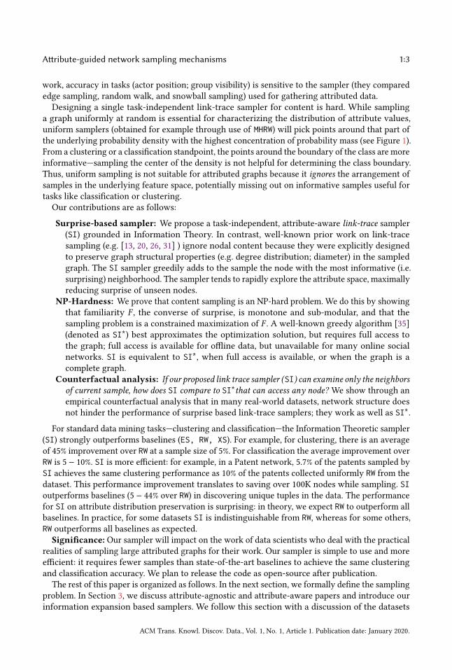
For standard data mining tasks—clustering and classification—the Information Theoretic sampler
(SI) strongly outperforms baselines (ES, RW, XS). For example, for clustering, there is an average
of 45% improvement over RW at a sample size of 5%. For classification the average improvement over
RW is 5 − 10%. SI is more efficient: for example, in a Patent network, 5.7% of the patents sampled by
SI achieves the same clustering performance as 10% of the patents collected uniformly RW from the
dataset. This performance improvement translates to saving over 100K nodes while sampling. SIoutperforms baselines (5 − 44% over RW) in discovering unique tuples in the data. The performance
for SI on attribute distribution preservation is surprising: in theory, we expect RW to outperform all
baselines. In practice, for some datasets SI is indistinguishable from RW, whereas for some others,
RW outperforms all baselines as expected.
Significance: Our sampler will impact on the work of data scientists who deal with the practical
realities of sampling large attributed graphs for their work. Our sampler is simple to use and more
efficient: it requires fewer samples than state-of-the-art baselines to achieve the same clustering
and classification accuracy. We plan to release the code as open-source after publication.
The rest of this paper is organized as follows. In the next section, we formally define the sampling
problem. In Section 3, we discuss attribute-agnostic and attribute-aware papers and introduce our
information expansion based samplers. We follow this section with a discussion of the datasets
ACM Trans. Knowl. Discov. Data., Vol. 1, No. 1, Article 1. Publication date: January 2020.

1:4 Suhansanu Kumar and Hari Sundaram
used in this paper in Section 5. In the three following sections, we present results for synthetic
and real-world datasets for baselines and our attribute-aware samplers for data characterization,
clustering, and classification tasks. In Section 9, we discuss our results and limitation of our work,
and in Section 10, we discuss prior work. We present our conclusions in Section 11.
2 PROBLEM STATEMENTWe seek to sample large attributed graphsG = (V ,E) in a task-independent manner. As a reminder,
our focus is in sampling nodal attributes related to content (e.g. gender), not in network attributes
(e.g. clustering coefficient). Nodal attributes include self-reported characteristics (e.g. gender, loca-
tion), or may be the result of a classifier (e.g. political affiliation; interests in fashion) operating on
the content associated with a person (e.g. tweets).
This paper focuses on link-trace samplers. We define link trace sampling as follows: given an
integer z and an initial seed node v ∈ V which initializes the sample S, a link trace sampler adds
nodes v to S such that there exists a nodew ∈ S where (w,v) ∈ E. The sampler stops when |S| = z.The goal of this paper is to develop a task-independent link-trace sampler that generates graph
samples S from a given static attributed graphG = (V ,E) with an aim to support data-mining tasks
on node content.
Assumptions:We make two assumptions. First, we assume that we sample static graphs; the
assumption works well in practice when the attributes are either immutable (e.g. ethnicity) or
slowly varying (e.g. political views). Second, we assume that the cost ci of acquiring attributes (e.g.
from an API call; the result of a classifier) for any node i is constant. Thus the total cost C incurred
by any link-trace sampler will be proportional to z, the desired sample size; that is, C = O(z). Sincez is common to all link-trace samplers considered in the paper, we ignore attribute collection costs.
3 SAMPLING ATTRIBUTED NETWORKSLet us denote the sample set of nodes collected from the network as S. Frontier nodes, denoted as
N (S), are the set of nodes that have at least one neighbor in S. We first discuss attribute-agnostic
link-trace sampling, followed by a detailed description of our proposed attribute-aware link-trace
samplers in Section 3.2.
3.1 Attribute AgnosticNow, we introduce well-known attribute-agnostic link-trace sampling algorithms; these algorithms
designed to improve over Snowball sampling (i.e. BFS) do not use the attribute (or content) of any
node to construct S: ForestFire (FF); expansion sampling (XS); Re-weighted Random Walk (RW) andMHRW. All these algorithms use a small seed set of vertices (θ ) to start data collection. Leskovec and
Faloutsos [26] proposed ForestFire, which explores a subset of a node’s neighbors according to a
“burning probability” pf ; At each iteration, the algorithm chooses a subset of the neighbors of the
current node v using a geometric distribution. While Forest Fire is superior to BFS, it suffers from a
degree bias [23].
Maiya and Berger-Wolf [31] proposed expansion sampling (XS), motivated by expander graphs.
XS adds nodes in a greedy manner in the direction of the largest unexplored region. Maiya and
Berger-Wolf [31] suggest that XS is relatively insensitive to seed set. While XS rapidly discovers
homogeneous communities, it does less well over dis-assortative networks since the XS is attribute
agnostic.
Re-weighted Random Walk sampling (RW) is a variant of the classic Random Walk algorithm,
re-weighted (since the random walk algorithm is biased towards high-degree nodes) to provide a
better estimate of the content distribution.
ACM Trans. Knowl. Discov. Data., Vol. 1, No. 1, Article 1. Publication date: January 2020.

Attribute-guided network sampling mechanisms 1:5
Edge sampling (ES) is commonly used for constructing social graphs from communication
networks by sampling the communication links [17]. Furthermore, ES has been shown to perform
well for sampling dynamic graphs [18]. Note that our implementation of ES is same as ES-i in [1]
after performing graph induction of the sampled nodes.
Metropolis-Hasting random walk sampling (MHRW) has an important asymptotic property: the
stationary distribution is uniform over all the nodes. Thus in principle, MHRW is equivalent to a
uniform random sampling of the graph for an infinite random walk. In practice, MHRW typically
requires sample sizes of O(N ), where N is the number of nodes in the graph, to achieve the
stationary distribution. It is challenging to use MHRW for internet scale graphs with billions of nodes,
where typical sample size |S| ≪ N (i.e. |S| ≈ 0.05 × N ). Graphs with strong community structure
are problematic when |S| ≪ N : MHRW tends to get stuck in a local community.
3.2 Attribute Aware, Surprise-based SamplersIn this section, we introduce a specific attribute-aware, surprise-based link-trace sampler, grounded
in Information Theory to sample the graph. Attribute-aware samplers use node attributes (content)
to determine the next node v to add to the current sample set S, by checking the content of this
node against the content of the nodes in the current sample. We abbreviate the phrase ‘Surprising
Information Sampler’ as SI in this paper.
At each step, SI adds to S, one optimal node v ∈ N (S). We assume that for each v ∈ N (S), wehave access to the content of the neighbors of v . We denote δv as the set of neighbors of v , that donot belong to S; we define the set ∆v ≡ δv ∪v . We refer to ∆v as the candidate set in this paper.
In the rest of this section, we show how to sample networks with discrete attributes, followed by
sampling networks with continuous attributes. We will use the Pareto-Optimal frontier to identify
optimal samples for networks with discrete and continuous attributes.
3.2.1 The Discrete Case: The surprise based sampler picks a node v to add to S, such that the
corresponding candidate set ∆v is most surprising.
Balanced sampling (BAL) is the simplest surprise-based sampler that adds one node at a time from
the frontier N (S), without looking at the neighbors of the node in N (S). That is, in the balanced
case, ∆v ≡ v , wherev ∈ N (S). The optimal nodev is such that its attributes have lowest probability
of occurrence in the sample S.In the more general case of the SI sampler, ∆v ≡ v∪δv . We define the surprise I∆v of a candidate
set ∆v (conditioned on S, for any single attribute) as follows:
I∆v =− ln P(∆v |S)
|∆v |. (1)
Where, P(∆v |S) is the probability of generation of attributes in ∆v given the distribution of
attribute values in set S. Assuming that the attribute values of the nodes vi ∈ ∆v are independent
(explained in more detail at the end of this section):
P(∆v |S) =∏
vi ∈∆v
P(vi |S) (2)
After algebraic manipulation, we can express Equation (1) after combining it with Equation (2)
as follows:
I∆v = −
r∑i=1
p∆v (i) lnpS(i) (3)
where, r is the number of distinct attribute values, p∆v (i) is the probability of attribute value i in the
candidate set ∆v , and pS(i) is the probability of the attribute value i in the sample set S. Both p∆v (i)
ACM Trans. Knowl. Discov. Data., Vol. 1, No. 1, Article 1. Publication date: January 2020.

1:6 Suhansanu Kumar and Hari Sundaram
and pS(i) are Maximum-Likelihood estimates. Notice that unseen attribute values (i.e. pS(i) = 0) in
S will cause Equation (1) to diverge; in general, SI prioritizes discovery of unseen attribute values.
Note that SI reduces to balanced sampling when ∆v ≡ v .We can interpret Equation (3) as proportional to the distance d(p∆v ,pS) of the point p∆v from
the plane
∑ri=1 xi lnpS(i) = 0. This is because we want to add a node v ∈ N (S), we compare every
candidate set ∆v for nodes v ∈ N (S), against the same sample set S. Thus, we pick the optimal
node v∗as follows:
d(p∆v ,pS
)=
−∑r
i=1 p∆v (i) lnpS(i)
| | lnpS | |, (4)
I∆v ∝ d(p∆v ,pS),
v∗ = argmax
v ∈N (S)
d(p∆v ,pS). (5)
That is, we pick v∗such that the candidate set ∆v∗
is maximally surprising given our current
knowledge pS. Where, we use p∆v to refer to the distribution of attribute values in the candidate
set ∆v , and where | | lnpS | | in Equation (4) is the L2 norm of the natural log of the distribution of
attribute values pS.To determine surprise when nodes have multiple attributes, we assume that attributes are
independent, a simplifying assumption that works well in practice. Thus Equation (5) generalizes
to:
v∗ = argmax
v ∈N (S)
∑A∈A
d(p∆v ,pS | A)
|A|. (6)
Where d(p∆v ,pS | A) is the distance of the set ∆v to the sample set S with respect to attribute
A. Equation (6) says that the surprise of a neighborhood ∆v is the average surprise over all attributes.
3.2.2 The Continuous Case: We compute surprise for continuous attributes, using a Normal
kernel density [39, 48] to estimate the continuous probability density P(S). We compute the
probability of generating ∆v from the sample set S for a multiple continuous attributes as follows:
P(∆v | S) ∝∏y∈∆v
∑x ∈S
1
|S|
1√2π |Σ|
exp
(−1
2
∆Tx,yΣ−1∆x,y
), (7)
where, ∆x,y = fx − fy and where fx and fy refer to the vector of continuous feature values
corresponding to nodes x ∈ S and y ∈ ∆v respectively. Equation (7) says that the conditional
probability of the set ∆v given S for a specific attribute is proportional to product of the conditionallikelihoods of each node y ∈ ∆v with each likelihood computed via the kernel density estimate of
P(fy | S).
Now using a standard kernel density estimation heuristic Σ = Σ̂/|S|, where Σ̂ is the diagonal ofthe sample covariance matrix in S; the heuristic reduces the influence of any single sample point
on the estimated density. Then, Equation (7) simplifies to:
P(∆v | S) ∝∏y∈∆v
∑x ∈S
1√2π |Σ̂| |S|
exp
(−
|S|d2(x ,y; f , Σ̂)
2
), (8)
where d(x ,y; f , Σ̂) is the weighted Euclidean distance measure for feature f , where we weightcomponents of feature f by the sample variance Σ̂; we only use the diagonal terms of the sample
co-variance matrix.
ACM Trans. Knowl. Discov. Data., Vol. 1, No. 1, Article 1. Publication date: January 2020.

Attribute-guided network sampling mechanisms 1:7
For any y ∈ ∆v , we can compute dmin, the minimum of the distances between y and the elements
of the set S. We take the negative log on both sides of Equation (8) and then divide by |∆v |, andthus − log P(∆v | S)/∆v ∝:
|S|d2min
2
+log(2π |S| |Σ̂|)
2
−1
|∆v |
∑y∈∆v
log
∑x ∈S
exp
−|S|(d2x,y − d2
min
)2
. (9)
Notice that by definition dx,y ≥ dmin(y,S). In general, for large values of |S| all except one terminside the summation tends to zero, implying that the third term goes to 0. In practice, the third
term is negligible when |S| ≥ 10. Thus, Equation (9) simplifies to:
I (∆v | S) ∝|S|d2
min
2
+log(2π |S| |Σ̂|)
2
(10)
Equation (10) says that the surprise of a set ∆v is well approximated by the minimum of the
distances of the elements belonging to the set ∆v to the set S. Notice that for any sample set Sin Equation (10), comparing surprise values across elements v ∈ V \ S only involves dmin. Thus, we
define surprise as:
I∆v = I (∆v | S) ≡ min
x ∈∆v,y∈Sd(x ,y), (11)
v∗ = argmax
v ∈N (S)
min
x ∈∆v,y∈Sd(x ,y), (12)
where we add node v∗with maximum surprise to the sample S.
We combine the surprise from the discrete and continuous attributes using a Pareto optimal
framework. We rank the sets ∆v,∀v ∈ N (S) based on Equation (12) and using Equation (6)
separately. We identify the set ∆v, v ∈ N (S) on the Pareto-optimal frontier that maximizes surprise
from both continuous and discrete attributes and add the corresponding optimal node v ∈ N (S) tothe sample S. The pseudo-code (Algorithm 1) summarizes the SI algorithm.
ALGORITHM 1: Pseudo-code for generalized SI sampler defined for an attributed network having both
discrete and continuous attributes
Input: Attributed Graph G, Budget zOutput: Sampled nodes S
1 S = ϕ ▷ sampled nodes
2 F = ϕ ▷ frontier nodes
3 for k = 1 to z do4 for v ∈ F do5 ∆v =
(N (v) \ S
)∪v
6 Idiscretev = I (∆v |S) ▷ Use Equation (1)
7 Icontinuousv = I (∆v |S) ▷ Use Equation (8)
8 Iv = (Idiscretev , Icontinuousv )
9 end10 v∗ = arдvPareto-optimal(Iv ) ▷ breaking the ties randomly
11 S = S ∪v∗
12 F = F ∪(N (v∗) \ S
)13 end
ACM Trans. Knowl. Discov. Data., Vol. 1, No. 1, Article 1. Publication date: January 2020.

1:8 Suhansanu Kumar and Hari Sundaram
Attribute Independence:We use a diagonal sample covariance Σ̂ in Equation (8), out of con-
cerns for stability of the covariance matrix. In real-world networks, the attributes of a node will
co-vary and are not independent. We will also see co-variation across neighbors due to homophily.
The challenge lies in incrementally estimating covariance (or equivalently the joint distribution for
the discrete case) amongst attributes given the current sample S. If we could estimate covariance
effectively, then we could use a variant of the familiar Mahanalobis distance which incorporates
the covariance matrix to compute the combined distance. In practice, we observe that when we use
the full covariance matrix (or the full joint for the discrete case), the estimates of the off-diagonal
elements of the covariance matrix do not stabilize unless the sample set S is large. The effect isto “push” the sampler in the wrong direction when |S| is small due to poor on-line covariance
estimates; the estimates are worse for skewed attribute distributions.
In this section, we discussed attribute-agnostic and attribute-aware sampling schemes. We
introduced the idea of surprise, grounded in Information Theory, as a framework to develop
sampling schemes. Our surprise based sampler SI adds one nodev ∈ N (S)with the most surprising
candidate set ∆v to S.
4 PROPERTIESNow we show that the attributed network sampling problem is NP-hard, by showing that “familiar-
ity," the converse of surprise, is monotone and submodular.
We define the familiarity F (v | S) of a node v given a sample set S as follows: F (v | S) ≡
exp(−I (v | S)). Intuitively, familiarity grows as surprise falls.
Lemma 4.1. The familiarity function F (·) is submodular.
Proof. The familiarity of a setAwith respect to another set B, F (A | B), is simplyminv ∈A I (v |B).Since we are interested in showing submodularity of the familiarity function F (·) for a fixed node
set V we shall abbreviate F (V \ S | S) as simply F (S). To prove submodularity, we have to show
that F (A ∪ {v}) − F (A) ≥ F (B ∪ {v}) − F (B) for all A ⊆ B and where A,B ⊆ V .
First, let us show monotonicity of F (·) using a distance argument as it is easy to follow. Addition
of a node v to S, affects only those nodes y ∈ V \ S that are closer to v than to any node in S. Letthe set of all such nodes be QS. The surprise of all nodes y ∈ QS falls, but importantly, the surprise
of all nodes z that belong to V \ S but not in QS remains the same. Thus surprise always falls, and
conversely, familiarity increases. That is, F (S ∪ x) ≥ F (S).Now assume that we have two sample sets A,B with A ⊆ B;A,B ⊆ V . Let us add a node v ∈ V
to A. Then, the addition of v to A only affects points x ∈ V \A that satisfy:
d(x ,v) < min
y∈Ad(x ,y)
.
Let us call this setQA. We can similarly defineQB corresponding to points affected by the addition
of v to set B. Notice that QB ⊆ QA since no point in QB can be missing from QA. Thus for y ∈ QB :
d(y,A) ≥ d(y,B),
d(y,A) − d(y,v) ≥ d(y,B) − d(y,v) (13)
Where the first statement is true because of monotonicity (surprise falls). Equation (13) states
that the decrease in distance is greater for the smaller set A thus implying F (A ∪ {v}) − F (A) ≥F (B ∪ {v}) − F (B) for all A ⊆ B. □
Lemma 4.1 captures the intuitive idea that as we gather more samples S, the rest of the unseendata V \ S becomes more familiar (less surprising) at a rate that decreases with sample size.
ACM Trans. Knowl. Discov. Data., Vol. 1, No. 1, Article 1. Publication date: January 2020.
Attribute-guided network sampling mechanisms 1:9
We can now restate the sampling problem as follows:
S∗ ≡ argmax
S⊆V , |S |=kF (V \ S | S). (14)
Thus, the sampling problem goal is to identify a set S of size k such that familiarity of the
remainder of the set V \ S is maximized.
Since the familiarity function F is submodular and monotone the sampling problem (Equa-
tion (14)) is a well-known NP-hard optimization problem [35], similar to the familiar influence
maximization problem [22]. We know from [35] that the greedy hill climbing algorithm (denoted
as ‘SI*’) approximates the optimal solution to within a factor of 1 − 1/e . The SI* algorithm is
impractical: it requires a complete access to the nodes in the graph.
When is SI equivalent to SI*? SI is equivalent to the SI* algorithm if either we have a full
access to all the nodes of the graph (e.g. offline data) or if the graph is a complete graph. In a later
section, we empirically examine the effect of network structure on the performance of surprise
based samplers (we call this “network resistance”). In many cases, the difference between the
counterfactual case when we assume that we have full network access and when we don’t is
negligible.
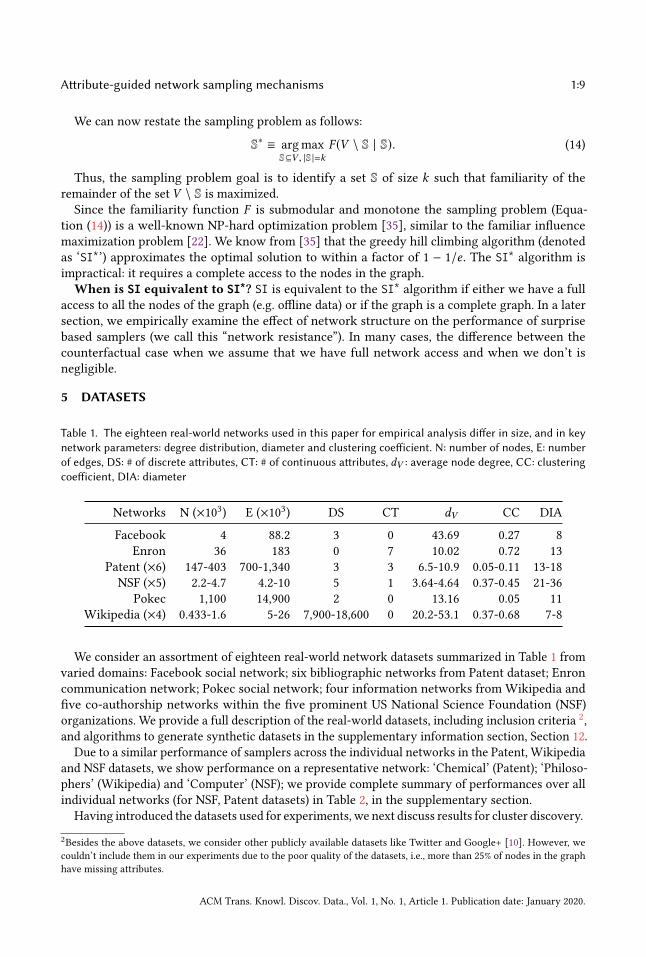
5 DATASETS
Table 1. The eighteen real-world networks used in this paper for empirical analysis differ in size, and in keynetwork parameters: degree distribution, diameter and clustering coefficient. N: number of nodes, E: numberof edges, DS: # of discrete attributes, CT: # of continuous attributes, dV : average node degree, CC: clusteringcoefficient, DIA: diameter
Networks N (×103) E (×103) DS CT dV CC DIA
Facebook 4 88.2 3 0 43.69 0.27 8
Enron 36 183 0 7 10.02 0.72 13
Patent (×6) 147-403 700-1,340 3 3 6.5-10.9 0.05-0.11 13-18
NSF (×5) 2.2-4.7 4.2-10 5 1 3.64-4.64 0.37-0.45 21-36
Pokec 1,100 14,900 2 0 13.16 0.05 11
Wikipedia (×4) 0.433-1.6 5-26 7,900-18,600 0 20.2-53.1 0.37-0.68 7-8
We consider an assortment of eighteen real-world network datasets summarized in Table 1 from
varied domains: Facebook social network; six bibliographic networks from Patent dataset; Enron
communication network; Pokec social network; four information networks from Wikipedia and
five co-authorship networks within the five prominent US National Science Foundation (NSF)
organizations. We provide a full description of the real-world datasets, including inclusion criteria2,
and algorithms to generate synthetic datasets in the supplementary information section, Section 12.
Due to a similar performance of samplers across the individual networks in the Patent, Wikipedia
and NSF datasets, we show performance on a representative network: ‘Chemical’ (Patent); ‘Philoso-
phers’ (Wikipedia) and ‘Computer’ (NSF); we provide complete summary of performances over all
individual networks (for NSF, Patent datasets) in Table 2, in the supplementary section.
Having introduced the datasets used for experiments, we next discuss results for cluster discovery.
2Besides the above datasets, we consider other publicly available datasets like Twitter and Google+ [10]. However, we
couldn’t include them in our experiments due to the poor quality of the datasets, i.e., more than 25% of nodes in the graph
have missing attributes.
ACM Trans. Knowl. Discov. Data., Vol. 1, No. 1, Article 1. Publication date: January 2020.

1:10 Suhansanu Kumar and Hari Sundaram
6 CLUSTER DISCOVERYIn this section, we examine the effects of link-trace sampling on cluster discovery. We first describe
the evaluation metrics and clustering algorithms used for discovering content clusters. Next, we
present the experimental results.
Given the plethora of distance metrics and algorithms used for defining clusters in content, we
use the standard well-known metrics and algorithms for simplicity and illustrative reasons. We
use the standard distance measures (Euclidean distance for continuous variables and the Jaccard
distance for nominal variables) and use a well-known k-prototype clustering algorithm [19]. This
clustering algorithm is a generalization of the k-means and k-modes algorithms, for content with
continuous and discrete attributes.
To understand the sampling effect independent of cluster size and quantity, we also vary the
number of clusters (k) in our experiments. For each such value of k , we cluster the ground truth
data. Then, after we sample the data with SI and the other baselines (XS, FF, ES, RW), we evaluatethe fraction of original clusters are present in the sample. The fraction of original clusters captured
in the sample shows how good a sampler is at discovering the original content clusters. Figure 2
shows the results, averaged over 100 runs.
We see from Figure 2 results for cluster coverage when the number of clusters k is 32, the surprise
based sampler (SI outperforms baseline samplers—re-weighted random walk (RW), forest fire (FF),expansion sampling (XS) and edge sampling (ES). The main reason is that SI sampler rapidly
explores the attribute value space, allowing us to cover niche clusters. However, the attribute-
agnostic samplers are heavily influenced by the distribution of the attributes over the network, and
the skewness in the clusters’ size. In datasets such as the Wikipedia, Pokec and Enron, clusters
show high skew, thus contributing to the relatively high performance improvement of SI over
baselines. Among the attribute-agnostic samplers, XS notably performs well when the attributes
are correlated with the community structure in networks such as Patent and NSF. Thus, XS which
is known for its high community coverage [31] also achieves relatively better cluster coverage.
On average, SI is moderately better than the second-best baseline samplers by and on Patent (3%)
and NSF (6%) respectively, much better on Enron and Facebook (12%) and significantly better on
Wikipedia (28%) and Pokec (37%) .
Let us examine the weaker performance of RW, FF and ES link-trace samplers on the Facebook
dataset. This dataset contains attributes with high assortativity, increasing the chance that nearby
nodes share the same attribute value as the current node. Since XS, ES and RW are attributeagnostic samplers that use only the network structure for exploration, high assortativity influences
0 10 20 30SAMPLE SIZE %
0.2
0.3
0.4
0.5
0.6
0.7
0.8
0.9
CLU
STE
R C
OV
ER
AG
E (@
K =
32)
RWSIFFXSES
0 10 20SAMPLE SIZE %
0.86
0.88
0.90
0.92
0.94
0.96
0.98
1.00
PATENT(CHEMICAL)
0 10 20SAMPLE SIZE %
0.4
0.5
0.6
0.7
0.8
0.9
1.0NSF(COMPUTER)
0 5 10SAMPLE SIZE %
0.0
0.2
0.4
0.6
0.8
1.0 WIKI(PHILOSOPHER)
0.0 0.5 1.0SAMPLE SIZE %
0.4
0.5
0.6
0.7
0.8
0.9
1.0POKEC
0 10 20SAMPLE SIZE %
0.4
0.5
0.6
0.7
0.8
0.9
1.0ENRON
Fig. 2. Cluster coverage for k = 32 clusters, on the Facebook, Patent, NSF, Wikipedia and Enron datasetsshows that SI outperforms competing samplers (RW, ES, FF, XS) at nearly all sampling sizes. Bands indicate95% CI.
ACM Trans. Knowl. Discov. Data., Vol. 1, No. 1, Article 1. Publication date: January 2020.
Attribute-guided network sampling mechanisms 1:11
24 8 16 32# OF CLUSTERS
0.3
0.4
0.5
0.6
0.7
0.8
0.9
1.0
CLU
STE
R C
OV
ER
AG
E
RWSIFFXSES
24 8 16 32# OF CLUSTERS
0.95
0.96
0.97
0.98
0.99
1.00
1.01 PATENT(CHEMICAL)
24 8 16 32# OF CLUSTERS
0.6
0.7
0.8
0.9
1.0
1.1 NSF(COMPUTER)
24 8 16 32# OF CLUSTERS
0.2
0.3
0.4
0.5
0.6
0.7
0.8
0.9
1.0WIKI(PHILOSOPHER)
24 8 16 32# OF CLUSTERS
0.60
0.65
0.70
0.75
0.80
0.85
0.90
0.95
1.00POKEC
24 8 16 32# OF CLUSTERS
0.4
0.5
0.6
0.7
0.8
0.9
dip at k=4 due to outliers in data
ENRON
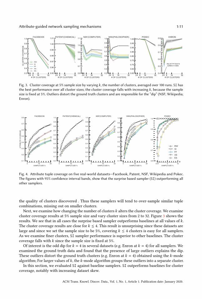
Fig. 3. Cluster coverage at 5% sample size by varying k , the number of clusters, averaged over 100 runs. SI hasthe best performance over all cluster sizes; the cluster coverage falls with increasing k , because the samplesize is fixed at 5%. Outliers distort the ground truth clusters and are responsible for the “dip” (NSF; Wikipedia;Enron).
0 10 20SAMPLE SIZE %
0.1
0.2
0.3
0.4
0.5
0.6
0.7
0.8
ATT
RIB
UTE
CO
VE
RA
GE
0 10 20SAMPLE SIZE %
0.0
0.1
0.2
0.3
0.4
0.5
0.6
0.7
0.8
0.9
1.0PATENT(CHEMICAL)
0 10 20SAMPLE SIZE %
0.0
0.1
0.2
0.3
0.4
0.5
0.6
0.7
0.8
0.9
1.0NSF(COMPUTER)
0 10 20SAMPLE SIZE %
0.1
0.2
0.3
0.4
0.5
0.6
0.7
0.8
0.9
1.0WIKI(PHILOSOPHER)
0.01 5 10SAMPLE SIZE %
0.6
0.7
0.8
0.9
1.0POKEC
RWSIFFXSES
Fig. 4. Attribute tuple coverage on five real-world datasets—Facebook, Patent, NSF, Wikipedia and Pokec.The figures with 95% confidence interval bands, show that the surprise based sampler (SI) outperforming allother samplers.
the quality of clusters discovered . Thus these samplers will tend to over-sample similar tuple
combinations, missing out on smaller clusters.
Next, we examine how changing the number of clusters k alters the cluster coverage. We examine
cluster coverage results at 5% sample size and vary cluster sizes from 2 to 32. Figure 3 shows the
results. We see that in all cases the surprise based sampler outperforms baselines at all values of k .The cluster coverage results are close for k ≤ 4. This result is unsurprising since these datasets are
large and since we set the sample size to be 5%, covering k ≤ 4 clusters is easy for all samplers.
As we examine finer clusters, SI sampler performance is superior to other baselines. The cluster
coverage falls with k since the sample size is fixed at 5%.
Of interest is the odd dip for k = 4 in several datasets (e.g. Enron at k = 4) for all samplers. We
examined the ground truth data and found that the presence of large outliers explains the dip.
These outliers distort the ground truth clusters (e.g. Enron at k = 4) obtained using the k-mode
algorithm; For larger values of k , the k-mode algorithm groups these outliers into a separate cluster.
In this section, we evaluated SI against baseline samplers. SI outperforms baselines for cluster
coverage, notably with increasing dataset skew.
ACM Trans. Knowl. Discov. Data., Vol. 1, No. 1, Article 1. Publication date: January 2020.

1:12 Suhansanu Kumar and Hari Sundaram
7 CONTENT COVERAGEIn this section, we evaluate how different samplers perform with respect to attribute tuple coverage
and attribute distribution.
Tuple coverage or unique entity discovery is a desirable goal in any empirical data analysis: to
ensure that all the unique entities in the data are present in the sample. For example, consider a
corporation trying to allocate its resources based on a demographic study is expected to sample
from all possible demographics of its customers or unique entities in its user study. To evaluate the
unique entity coverage for each sampler, we compute the fraction of unique tuples (for datasets
with discrete attributes) present in the sample as the metric. Thus, Enron dataset which comprises
of only continuous attributes is not considered in this study.
Figure 4 shows the results. First, across all datasets the surprise based sampler (SI) outperforms
baselines. Second, none of the samplers reach 100% coverage even for large sample sizes (∼20%) for
the Facebook, Patent and Wikipedia datasets. This is because all three of these datasets have high
attribute cardinality and these attributes exhibit skew. Notice further, that the attribute-agnostic
samplers fares poorly in comparison to SI in some datasets—for example, SI outperforms the
baseline samplers by 26% in the Facebook dataset and by 14% in the Patent dataset. High attribute
skew is the best explanation—since the baseline sampler are agnostic to attributes, they are more
likely to sample attribute values that appear more often, penalizing tuples that contain attribute
values that appear infrequently. For the Pokec dataset, all samplers have good attribute value
coverage since the attribute cardinalities are lower than the other two datasets. Averaged over all
real-world datasets, SI outperforms the state-of-the-art samplers by 14%.
Samplers vary in how well they preserve attribute distribution. In Figure 5, we compare the K −Sstatistic, averaged across the different attributes, for each of the six datasets. A small K − S statistic
implies that the sampler preserves the underlying distribution well in the sample. Across all the
datasets, unsurprisingly, the uniform attribute sampler would have performed the best since UNI is
an unbiased estimator of the attribute distribution. In general, random walk (RW) based samplers are
the best link-trace samplers, since asymptotically, the probability of visiting each node in the graph
is uniform. The surprise based sampler (SI) gives a mixed performance for capturing the attribute
distribution. We don’t expect SI to perform well since the sampler goal is to maximize familiarity.
What is interesting is that the differences between RW and SI are negligible on theWikipedia dataset.
Expansion sampling (XS) works well on the Facebook, Enron and Wikipedia datasets, but not on
the Patent dataset. We note that Patent has significantly lower clustering coefficient (c.f. Table 1)
0 10 20 30SAMPLE SIZE %
0.00
0.05
0.10
0.15
0.20
0.25
CO
NTE
NT
KS
-STA
T (@
K =
32)
FACEBOOKRWSIFFXSES
0 10 20SAMPLE SIZE %
0.00
0.05
0.10
0.15
0.20
0.25
PATENT(CHEMICAL)
0 10 20SAMPLE SIZE %
0.0
0.1
0.2
0.3
0.4
0.5 NSF(COMPUTER)
0 5 10SAMPLE SIZE %
0.00
0.05
0.10
0.15
0.20
0.25
WIKI(PHILOSOPHER)
0 0.5 1SAMPLE SIZE %
0.00
0.05
0.10
0.15
0.20
0.25
POKEC
0 10 20SAMPLE SIZE %
0.00
0.05
0.10
0.15
0.20
0.25
ENRON
Fig. 5. Attribute Distribution: The K − S statistic (lower is better), averaged across attributes, for differentdatasets. Notice that while uniform sampling based link-trace sampler RW performs the best, the differencesare negligible on the Wikipedia dataset. SI is better than RW or ES for the Enron dataset.
ACM Trans. Knowl. Discov. Data., Vol. 1, No. 1, Article 1. Publication date: January 2020.

Attribute-guided network sampling mechanisms 1:13
than the other networks. Since XS rapidly explores the network helped by the presence of clusters,
networks with low-clustering coefficients may hinder rapid exploration.
8 CLASSIFICATIONIn this section, we present our results for classification and regression. First, we describe the
experimental setup used for the experiments, followed by the results.
We use different evaluation metrics for predicting discrete and continuous target attributes. We
evaluate prediction of discrete attributes through the weighted F1 score, and we use the Pearson’s
R2coefficient to evaluate prediction of continuous attributes.
We pick attributes to predict for the classification and regression tasks using the following
principles. First, across the three real-world datasets, we pick attributes of varying cardinality to
predict target attribute to help us understand the effect of cardinality. Second, as would be natural
in any classification task, we pick attributes to predict that co-varied with the features that are used
as input to the classifier or regressor. Thus, for the Facebook dataset, we predict “gender” using
feature set “locale”, “education type”. For the Patent dataset, we predict attribute “country” as the
discrete attribute and “number of claims” as the continuous attribute on which we regress using
the rest of the attributes as features. For the NSF dataset, we predict “duration” of NSF awards
awarded to the NSF investigators using investigator attributes such as “number of awards won”
and “number of project’s PI”.
The results in Figure 6 reveal that SI is a better choice for sampling networks for content than
the state-of-the-art link-trace samplers for classification tasks (Facebook and Patent datasets);
SI performance is indistinguishable from other samplers for the regression task (Patent dataset;
number of claims). For the Facebook dataset, SI achieves an 18% relative gain with the weighted F1score over RW variants. For the Patent dataset, we note that SI is better than baseline samplers by a
margin of over 2% for discrete attribute “country”. The overall weighted F1 performance of almost
all samplers is high due to the skewed distribution of the target attribute (i.e. “country" attribute
skew = 0.70). We show the prediction of “number of claims” in the Patent dataset as an example
of regression task—there is no significant difference among the samplers. For the NSF dataset, SIoutperforms its competition by over 10% at predicting the “cumulative duration” of NSF awards
awarded to NSF investigators.
We show additional results in Table 2 in the supplementary information section.Table 2 shows
that the SI sampler consistently outperforms state of the art link-trace samplers such as XS, RW,FFand ES for four content tasks: clustering, classification, regression, and attribute-value discovery.
1 5 10SAMPLE SIZE %
0.300
0.325
0.350
0.375
0.400
0.425
0.450
0.475
0.500
WE
IGH
TED
F1
FACEBOOK (GENDER)
1 5 10SAMPLE SIZE %
0.70
0.75
0.80
0.85
0.90
0.95
1.00
WE
IGH
TED
F1
PATENT (COUNTRY)
1 5 10SAMPLE SIZE %
0.350
0.375
0.400
0.425
0.450
0.475
0.500
0.525
0.550
R2
SC
OR
E
PATENT (#CLAIMS)
RWSIFFXSES
1 5 10SAMPLE SIZE %
0.4
0.5
0.6
0.7
0.8
0.9
1.0
R2
SC
OR
E
NSF (#DURATION)
Fig. 6. Classification performance on different datasets. The SI sampler has significantly better classificationperformance than baseline samplers. There is no significant difference in performance of samplers forregression task in the Patent dataset. Bands show CI = 95%.
ACM Trans. Knowl. Discov. Data., Vol. 1, No. 1, Article 1. Publication date: January 2020.

1:14 Suhansanu Kumar and Hari Sundaram
9 DISCUSSIONWe begin in Section 9.1 by analyzing the performance of the surprise based sampler (SI) and then
in Section 9.2, we examine the issue of “network resistance.” Finally, in Section 9.3, we discuss
limitations.
9.1 Why does SI work well?The surprise based sampler SI outperforms baselines for classification and cluster discovery. To
understand why, we examine Figures 1 and 4. Figure 1 shows that the surprise based sampler tends
to uniformly cover the underlying density, whereas the baseline samplers tends to pick data near the
center of the density (where the tuples are more likely). Figure 4 compares sampler tuple coverage,
and shows that the SI sampler, consistent with its bias, tends to pick up less common tuples. Taken
together, both Figures 1 and 4 imply that the SI sample will tend to cover the boundary of the
class conditional density first. For the same number of samples, SI sampler will have covered
the less common examples of a class, whereas the attribute-agnostic samplers would cover the
more common instances. Our work indicates (c.f. Figure 1), that link-trace samplers that attempt to
sample content uniformly in an effort to mimic UNI (e.g., RW, MHRW) may be weaker for clustering
and classification tasks, since they ignore the underlying geometry (i.e. arrangement of samples in
the underlying metric space) which is important to identify the most informative samples for these
tasks. Thus, we ought to expect that classifiers that use data from the SI sampler to exhibit lower
generalization error than the uniform sampler (and samplers like RW, MHRW). A similar explanation
holds for cluster coverage results in Figure 2.
9.2 Examining “Network Resistance”Submodularity of familiarity F (v | S), discussed in Section 4 is a key concept. We remind the
reader that since F is submodular and monotone, the sampling problem is an NP-hard optimization
problem. The greedy algorithm (SI*), that adds to S the most surprising node in the entire graph,approximates the optimal S∗ within a factor of 1 − 1/e [35]. The SI*algorithm is useful for offline
graph datasets where we have random access, or when the graph is a complete graph. Since online
social networks disallow random access, data scientists use link-trace samplers.
A counterfactual:What if the SI sampler could pick any node fromV \S like the SI*algorithmand not be restricted to pick a node from N (S), the neighborhood of the current sample S?
1 10 20 30SAMPLE SIZE %
0.0
0.2
0.4
0.6
0.8
1.0
CLU
STE
R C
OV
ER
AG
E (@
K =
32)
SI + vSI*SIBAL
1 10 20SAMPLE SIZE %
0.75
0.80
0.85
0.90
0.95
1.00PATENT(CHEMICAL)
1 10 20SAMPLE SIZE %
0.5
0.6
0.7
0.8
0.9
1.0NSF(COMPUTER)
1 5 10SAMPLE SIZE %
0.0
0.2
0.4
0.6
0.8
1.0WIKI(PHILOSOPHER)
0.01 0.50 1.00SAMPLE SIZE %
0.60
0.65
0.70
0.75
0.80
0.85
0.90
0.95
1.00POKEC
1 10 20SAMPLE SIZE %
0.60
0.65
0.70
0.75
0.80
0.85
0.90
0.95
1.00ENRON
Fig. 7. Comparing the counterfactual case when all nodes are accessible (i.e. SI*) against the case whenthe sampler needs to traverse the network (i.e. link-trace). In general, when random access is possible(counterfactual, SI*), the results are better than with link-trace. Interestingly, this is not always true (e.g.Wikipedia). This is because the submodular optimization problem is task-agnostic: it maximizes familiarity,but does not optimize for the clustering task.
ACM Trans. Knowl. Discov. Data., Vol. 1, No. 1, Article 1. Publication date: January 2020.

Attribute-guided network sampling mechanisms 1:15
We examine the consequence empirically by comparing the counterfactual case (i.e. SI*) againstthree baseline link-trace based samplers. The first baseline is SI, the one extensively examined in
this paper. The second baseline, we term balanced (‘BAL’) computes the surprise of nodes v ∈ N (S),without examining N (v), the network neighborhood ofv . The final baseline, which we term SI +∆v ,examines the neighborhood ∆v,∀v ∈ N (S), and adds the entire neighborhood ∆v to the sample Scorresponding to v∗ ∈ N (S).Figure 7 shows the results. The SI*algorithm is better for Facebook, marginally better for NSF,
marginally worse for Enron, and much worse for Wikipedia. Notably, the difference in performance
is not statistically significant for Enron, Patent, Pokec, and NSF, implying that for these networks,
link-trace samplers do not suffer a loss of performance. The disparity for Facebook is more salient,
implying that the network structure is preventing link-trace samplers from finding the optimal
sample set.
Wikipedia is a highly unusual dataset. It has a large number of binary attributes (7,969) compared
to just 1,564 nodes. Furthermore, the attributes in Wikipedia are highly asymmetric binary variables
(on average, there are only five attributes with val=TRUE, per node). As a consequence, the surprisecreated by almost every node v ∈ N (S) in the frontier set is maximally surprising implying that
the SI*algorithm picks a node at random from N (S). Since SI uses the neighborhood ∆v , there arefewer nodes in N (S) that are maximally surprising, leading to better samples for the clustering
task. We want to remind the reader that the definition of surprise is task agnostic. Thus, it should
not be odd that the SI*algorithm which approximates the solution to Equation (14) within 1 − 1/emay yield samples less suited to the clustering task on some datasets.
9.3 LimitationsNow, we discuss four limitations of this work. First, the theoretical analysis assumes that we have
no missing values; while SI works in practice when nodes have missing values (one can use the
expected value, for example), a noise model to estimate the error in surprise in networks with
missing values will be helpful. Second, the time and space complexity of SI is higher than random
walk based samplers such as RW. The incremental update complexity is O(µ log |S|), where µ is
the mean degree of the network, while it is O(1) for RW. We can mitigate this issue in two ways.
One way is to adopt a “lazy evaluation” for submodular maximization [28] that shows upto 700×
speed-up in real-world datasets. Another approach is to use data structures that include information
about neighbors in each node, an approach used in decentralized peer-to-peer networks. Third,
our model of link-trace sampling is limited: many social networks allow us to make queries on the
content and return network nodes that satisfy the query. Extending our sampling framework to
incorporate a more rich query model would be interesting. Finally, by design, we examine only
‘content’ attributes of a node, not the network properties; investigating samplers that sample for
nodal network properties in addition to nodal content would be significant for data mining problems
requiring both local network properties and node content.
10 RELATED WORKWe study the prior work corresponding to sampling: networks; content and joint network-content.
Representative subgraph sampling aims to construct a sampled subgraph that has a networkstructure very similar to that of the original network. Forest Fire [26] preserved several key network
structure characteristics. Hubler et al. [21] showed via Metropolis algorithm that prior knowledge
of the network can help in obtaining better representative samples. In contrast, our objective is to
support content analysis, and not network structure.
Another line of research on network sampling focuses on understanding the biases of existing
samplers and ways to obtain uniform samples. Kurant et al. [23] quantified the degree bias for
ACM Trans. Knowl. Discov. Data., Vol. 1, No. 1, Article 1. Publication date: January 2020.

1:16 Suhansanu Kumar and Hari Sundaram
several network samplers and proposed new ways to correct them. Costenbander et al. [7] did a
thorough analysis of the effect of noise (sample) on network centrality estimation. Gjoka et al. [12]
implemented the proposed uniform link-trace samplers on the very massive Facebook network
to validate the results. Chiericetti et al. [6] proposed an efficient random walk sampling strategy
for sampling according to a prescribed distribution. Maiya et al. [31] exploited the bias instead of
correcting it to design expansion-based samplers. We exploit the bias of entropy-based samplers
to more effectively explore the underlying metric space of the node features, yielding improved
classification and clustering performance.
There is research on sampling content from an unknown population distribution. Our objectiveresembles these surveys that try to estimate the underlying content characteristics. However, most
the well-known samplers such as Poisson sampling, stratified sampling, etc. [38] require random
access to the nodes in the dataset. In some cases, prior knowledge is required and these methods
typically fail to capture network structure. While research in graph visualization [42], has examined
the issue of node interestingness using intuitive measures, our idea is grounded in Information
Theory for a principled approach to network sampling.
Sociological and statistical studies on social networks such as friendship recommendation, link
prediction, attribute inference, type distribution, etc. implicitly rely upon both content and network.
However there is little prior work on understanding the effect of sampling on joint network andcontent characteristics. Li et al. [30] studied five different sampling strategies for node-type and link-
type distribution preservation. Yang et al. [49] proposed a semantic sampling strategy, Relational
Profile sampling, that preserves the semantic relationship types in a heterogeneous networks. Park
et al. [37] remarked about the inefficiency of the existing network samplers in estimating node
attributes. Wagner et al. [47] showed the sensitivity of existing samplers while sampling attributes
from attributed networks. Bhuiyan et al. develop graph samplers for estimating the frequency
of motifs in large graphs [4]. However, the previous works have been specific to objectives such
as attribute distribution, node-type preservation, frequency estimation [4, 14]. We propose new
samplers for identifying content in networks for clustering and classification, along with proofs of
NP-hardness. Furthermore, unlike active sampling literature that samples a network to estimate
parameters [41], our goal is to sample graphs in a task-independent manner.
Other complementary approaches to graph sampling include: a) graph compression [3, 9] to
speed up the graph algorithms; b) graph sparsification [45] to reduce the size of large graphs to
manageable size; and c) graph generation models [34, 40, 43] to generate synthetic samples of the
original graph. However, these methods require complete access to the underlying graph or the
underlying graph properties. Since complete access to online social networks like Facebook and
Twitter is typically not possible for researchers, it restricts us to work with graph crawlers or graph
samplers.
There exist several definitions of information and surprise in literature. For example, focused
crawlers [5] or hidden population samplers [16] are used to sample specific parts of the population.
Thus, the information is limited to a portion of the graph in such scenarios. Similarly, active-learning
based samplers [11, 33] focus on sampling a targeted set of nodes and do not pertain to the entire
graph property. In contrast to these targeted samplers, we aim to preserve the content of the entire
network. Further, we note that the idea of surprise-based data sampling is not new. It has been
used in the fields of graph visualization, information retrieval, active learning, etc. For example, in
the classical database search, Sarwagi [44] used the Maximum Entropy principle to model a user’s
knowledge and aid the user in exploring OLAP data cubes. In graph visualization work [42], the
authors chose to highlight the neighbors that are most surprising in information (KL divergence
of feature distribution from the background distribution). Our work borrows the idea of surprise
ACM Trans. Knowl. Discov. Data., Vol. 1, No. 1, Article 1. Publication date: January 2020.

Attribute-guided network sampling mechanisms 1:17
defined in terms of entropy and stratified sampling principles to design a novel attributed-network
sampler.
11 CONCLUSIONThis paper introduced a novel task-independent sampler for attributed networks. The problem is
essential because while data mining tasks on network content are common, sampling on internet
scale networks is expensive. While uniform sampling based link-trace samplers RW and MHRW areattractive, since it provides an unbiased estimate of the attribute distribution; however the estimate
is only achievable at asymptotic limits. Hence, link-trace samplers are widely used. However, these
samplers are attribute agnostic, and focus on preserving salient properties of network structure,
not node content. We showed three contributions. First, we introduced SI, an attribute-aware
sampler grounded in Information Theory. We proved that the sampling problem was NP-hard,
by showing that familiarity, the converse of surprise was monotone and submodular. Third, we
showed via an empirical counterfactual analysis that in many real-world datasets, SI performs
(on a clustering task) as well as the best-known approximation [35] to the NP-hard problem. We
showed strong experimental results for a variety of datasets, demonstrating that surprise-based
samplers are sample efficient and outperform both random sampling and baseline attribute-agnostic
samplers by a wide margin. Our sampler will impact on the work of data scientists who deal with
the practical realities of sampling large attributed graphs for their work. Our sampler is simple to
use and more efficient: it requires fewer samples than state-of-the-art baselines to achieve the same
clustering and classification accuracy. In future work, we plan to extend our sampler to dynamic
graph settings, as well as consider richer query models.
12 APPENDIXIn Section 12.1, we provide the selection and pre-processing steps used for preparing the real-
world attributed networks. sub: In Section 12.3, we briefly summarize experimental results over
synthetic network datasets. The experimental code for SI and baseline samplers along-with code
for generating synthetic datasets shall be made available at https://github.com/anonymous.
12.1 Full description of real-world datasetsWe experiment on real-world network datasets that are not sparse—in other words, most nodes
have values for attributes of interest (sparsity threshold is 75%). Datasets that have a significant
number of nodes with missing attribute values (e.g. Google+ and Twitter datasets cited in Yang et al.
[50]) are problematic since we don’t know if the missing values are due to improper sampling of the
original graph. Since the focus of this work is attribute based sampling, we do not consider datasets
with significant missing values. However, we note that practitioners can use missing attribute
prediction [15] as an alternative attribute for executing SI samplers.
Facebook [32] and Pokec [46] are social networks where nodes are users having attributes
such as “gender”, “age” and “language”. Patents are a bibliographic dataset [27] with attributes of
patents such as “category” and “citations made” by the patents; we analyze six patent sub-networks:
Computer & Communications, Chemical, Drugs & Medical, Electrical & Electronic, Mechanical and
other utility categories like textile. The Enron email network [29] has attributes associated with each
participant. The Wikipedia dataset [2] has four sub-networks: philosophers, physicists, chemists,
and statisticians. For example, the philosopher sub-network is an information network comprising
of web-pages of well-known philosophers, where each page is a node and where edges refer to the
hyperlinking patterns among the web-pages. This dataset is unusual: the number of attributes per
node is greater than the number of nodes; each attribute is boolean and asymmetric (i.e. one value
is much more likely than the other). The NSF grant co-authorship networks correspond to five
ACM Trans. Knowl. Discov. Data., Vol. 1, No. 1, Article 1. Publication date: January 2020.

1:18 Suhansanu Kumar and Hari Sundaram
NSF divisions—1. Division of Information & Intelligent Systems; 2. Computer & Network Systems;
Chemical; 3. Biology and Environment & Transport Systems; 4. Civil, Mechanical & Manufacturing
Innovation and 5. Division of Research on Learning.
In order to obtain fair comparison across all link-based samplers, we perform our experiments
on the largest component of the undirected versions of these networks. This prepossessing step
ensures that every node is accessible to all samplers.
The networks also differ in attribute cardinality, attribute type (discrete vs. continuous attributes),
data skew and assortivity (e.g. Patent category is most assortative with value 0.64). The Facebook
network [32] is a friendship network. This network has discrete attributes of moderate cardinality
and low assortativity (maximum assortativity is 0.34 for locale). The patent network [27] is the
citation network of all patents granted by the US from 1963 till 1999. The attributes have high
discrete cardinality for some of the attributes such as country of origin and continuous attributes
like claims and citations that have a large range. Most of the attributes are dis-assortative with the
exception of category and assignee type whose the assortativity values are 0.64 and 0.25 respectively.
In the Enron network [29], each node is an individual and edges represent communication between
the corresponding individuals. The attributes vary greatly in range but have low assortativity
values. Pokec [46] is another social network from Slovakia. We use two discrete attributes: “age”
and “gender” which are mixed dis-assortatively (-0.12) and assortatively (0.366) respectively. These
attributes have low cardinality. The attribute “gender” is dis-assortatively mixed (-0.12) while “age”
groups are homophilic (0.366).
12.2 Generation of Synthetic DatasetsWe use the Lancichinetti-Fortunato-Radicchi (LFR) [24] algorithm to generate artificial networks of
size N = 1000, with mixing coefficient µ = 0.1. This value of the mixing coefficient synthesizes
real-world networks with strong community structure. We refer to such networks as LFR (µ =0.1),
in the rest of the paper.
Three essential characteristics are important for the generation of synthetic attributed networks:
content skew, purity and assortativity. Cluster skew refers to the skew in attribute cluster sizes. We
use entropy H (C) over the cluster size to measure cluster skew, where, C = {C1,C2, . . . ,Ck }. The
purity p of the cluster refers to the separability or the degree of overlap of the attribute distributions
among clusters. Assortativity measures the degree to which links between nodes with similar
attributes differs from the same set of nodes but with random edges [36].
To generate the desired attributed graph, first we generate the “bare” network without attributes.
Then, for a specified skew, we generate content clusters. Finally, given an assortativity value, we
map the synthesized data to nodes in the network through a label propagation algorithm that
terminates when the algorithm achieves the target assortativity. We shall refer the interested
readers to the code provided for implementation.
12.3 Experiments on Synthetic NetworksWe briefly summarize due to space limitations, our extensive experiments on Synthetic networks.
We conducted analyses using standard synthetic network benchmarks (LFR µ = 0.1) [24]), generatedwith a different skew, purity and assortativity parameters.
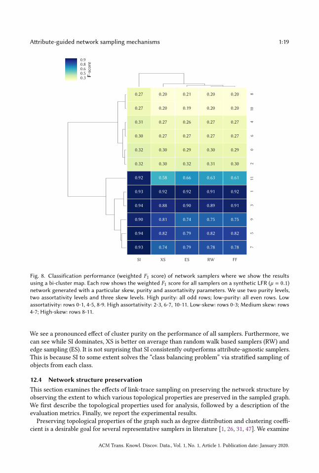
We use a bi-cluster map Figure 8 to show the classification results on synthetic networks. The
bi-clustering map helps us identify similar performances across samplers and identify conditions
where these similarities occur.
The SI sampler outperforms all baselines on synthetic networks. Notably, SI outperforms baseline
samplers with increasing skew, and in particular, by 30-40% at high skew. The table shows that skew
and purity play more significant role in sampler classification performance than does assortativity.
ACM Trans. Knowl. Discov. Data., Vol. 1, No. 1, Article 1. Publication date: January 2020.
Attribute-guided network sampling mechanisms 1:19
SI XS ES RW FF
810
46
02
111
39
57
0.27 0.20 0.21 0.20 0.20
0.27 0.20 0.19 0.20 0.20
0.31 0.27 0.26 0.27 0.27
0.30 0.27 0.27 0.27 0.27
0.32 0.30 0.29 0.30 0.29
0.32 0.30 0.32 0.31 0.30
0.92 0.58 0.66 0.63 0.61
0.93 0.92 0.92 0.91 0.92
0.94 0.88 0.90 0.89 0.91
0.90 0.81 0.74 0.75 0.75
0.94 0.82 0.79 0.82 0.82
0.93 0.74 0.79 0.78 0.78
0.30.50.60.80.9
F-sc
ore
Fig. 8. Classification performance (weighted F1 score) of network samplers where we show the resultsusing a bi-cluster map. Each row shows the weighted F1 score for all samplers on a synthetic LFR (µ = 0.1)network generated with a particular skew, purity and assortativity parameters. We use two purity levels,two assortativity levels and three skew levels. High purity: all odd rows; low-purity: all even rows. Lowassortativity: rows 0-1, 4-5, 8-9. High assortativity: 2-3, 6-7, 10-11. Low-skew: rows 0-3; Medium skew: rows4-7; High-skew: rows 8-11.
We see a pronounced effect of cluster purity on the performance of all samplers. Furthermore, we
can see while SI dominates, XS is better on average than random walk based samplers (RW) and
edge sampling (ES). It is not surprising that SI consistently outperforms attribute-agnostic samplers.
This is because SI to some extent solves the “class balancing problem” via stratified sampling of
objects from each class.
12.4 Network structure preservationThis section examines the effects of link-trace sampling on preserving the network structure by
observing the extent to which various topological properties are preserved in the sampled graph.
We first describe the topological properties used for analysis, followed by a description of the
evaluation metrics. Finally, we report the experimental results.
Preserving topological properties of the graph such as degree distribution and clustering coeffi-
cient is a desirable goal for several representative samplers in literature [1, 26, 31, 47]. We examine
ACM Trans. Knowl. Discov. Data., Vol. 1, No. 1, Article 1. Publication date: January 2020.

1:20 Suhansanu Kumar and Hari Sundaram
Dataset Task SI ∆ ES ∆ RW ∆ FF ∆ XS
NSF Attribute coverage 0.41 (±0.07) ↓20.41%(±2.14) ↓26.37%(±0.86) ↓25.00%(±1.01) ↓ 7.08%(±2.57)
Cluster coverage 0.95 (±0.03) ↓ 9.68%(±1.41) ↓10.19%(±2.10) ↓ 8.81%(±1.93) ↓10.94%(±3.29)
Regression 0.92 (±0.02) ↓ 4.90%(±1.46) ↓ 6.03%(±1.79) ↓ 6.21%(±2.36) ↓76.50%(±39.56)
Patent Attribute coverage 0.67 (±0.01) ↓69.67%(±1.68) ↓72.79%(±1.78) ↓68.47%(±1.47) ↓62.96%(±1.77)
Cluster coverage 0.99 (±0.00) ↓ 1.08%(±0.50) ↓ 1.10%(±0.51) ↓ 1.21%(±0.56) ↓ 1.54%(±0.81)
Classification 0.86 (±0.04) ↓16.93%(±1.12) ↓17.27%(±1.06) ↓16.60%(±1.08) ↓16.14%(±1.21)
Regression 0.48 (±0.02) ↓ 1.57%(±0.32) ↓ 3.53%(±0.27) ↓ 2.21%(±0.13) ↑ 0.54%(±0.12)
Wikipedia Attribute coverage 0.95 (±0.01) ↓43.46%(±5.30) ↓47.73%(±4.97) ↓37.63%(±1.43) ↓19.55%(±5.12)
Cluster coverage 0.39 (±0.07) ↓ 2.80%(±1.75) ↓ 7.30%(±0.74) ↓ 6.39%(±2.45) ↓28.79%(±12.88)
Table 2. SI’s performance (± standard deviation) over the current state-of-the-art samplers (ES, RW, FF, XS)over a span of data-mining tasks—clustering, classification, regression, unique attribute-value discovering—measured over a three network suites: NSF, Patent, and Wikipedia at 5% sampling rate. A column named ∆Xindicates relative performance of sampler X over SI. Thus, the column ∆ ES reports for example, the value100 × ES−SI
SI. SI is superior to (RW, ES, FF, XS) over all sub-networks belonging to these three datasets.
how the attribute-agnostic and attribute-aware samplers preserve several graph topological proper-
ties. We evaluate the samplers on preserving the four widely-used topological properties—degree,
clustering coefficient, path-length, and assortativity [36]. To evaluate the samplers’ performance,
we apply KS statistic between the sampled graph and the original graph’s distribution of topologi-
cal properties (for the degree, clustering coefficient, and path-length); we use the mean absolute
difference to evaluate assortativity. For example, the degree distribution property is evaluated
using D =maxk |F (k) − F ′(k)|, where k is over the range of the node degree, and F and F ′are the
cumulative distribution of node degrees in the sampled graphGS and original graphG respectively.
Table 3 shows the results. As expected, attribute-agnostic samplers, including FF and XS designedspecifically for preserving network structure, perform well on preserving properties like the degree
and clustering coefficient. Interestingly, SI performs comparatively similar to some of the attribute-
agnostic samplers like BFS and is much better than some samplers like ES. We note that this work
(SI) focuses on preserving content; as the future work, it will be interesting to include topological
properties in the design of SI.For preserving assortativity, we observe that no sampler distinctly outperforms others. Recent
work [47] has explored the tradeoff of different samplers at preserving the network-content rela-
tionship. However, it remains an open problem to design an efficient sampler that can preserve
network-content relationship over a wide range of networks.
12.5 Runtime analysisIn Figure 9, we observe the runtime for different samplers
3of attribute-agnostic and attribute-aware
samplers on the Facebook network. As noted in Section 9.3, SI experiences higher time complexity
due to the processing of the attributes and the frontier nodes in addition to the sampled nodes. ESrandomly samples edges from the graph and is the fastest sampler. Attribute-agnostic samplers like
XS which maximally explore the network structure by sampling the maximal degree node from the
frontier set incur the highest time complexity among the attribute-agnostic samplers. In summary,
we observe that SI sampler, even though a constant factor (2-3×) slower than the attribute-agnostic
samplers, is very useful for sampling content.
3We implemented all described algorithms in Python using Igraph package [8]. All tests were performed on a computer
with 16 GB RAM and 2.5 GHz Intel Core i7 processor. We performed 100 runs for each sampler.
ACM Trans. Knowl. Discov. Data., Vol. 1, No. 1, Article 1. Publication date: January 2020.

Attribute-guided network sampling mechanisms 1:21
Dataset Topological property SI ES RW FF XS
Facebook Degree 0.454 (± 0.03) 0.403 (± 0.11) 0.334 (± 0.01) 0.336 (± 0.01) 0.666 (± 0.11)
Clustering coefficient 0.299 (± 0.07) 0.295 (± 0.04) 0.257 (± 0.03) 0.234 (± 0.00) 0.522 (± 0.09)
Path length 0.326 (± 0.02) 0.781 (± 0.04) 0.636 (± 0.01) 0.546 (± 0.03) 0.100 (± 0.08)
Assortativity 0.141 (± 0.01) 0.088 (± 0.02) 0.091 (± 0.01) 0.081 (± 0.07) 0.122 (± 0.00)
Patent Degree 0.051 (± 0.01) 0.074 (± 0.01) 0.080 (± 0.00) 0.185 (± 0.03) 0.114 (± 0.04)
Clustering coefficient 0.088 (± 0.01) 0.075 (± 0.00) 0.080 (± 0.00) 0.188 (± 0.08) 0.040 (± 0.00)
Path length 0.479 (± 0.10) 0.688 (± 0.11) 0.442 (± 0.07) 0.916 (± 0.22) 0.554 (± 0.27)
Assortativity 0.003 (± 0.00) 0.081 (± 0.01) 0.077 (± 0.02) 0.067 (± 0.01) 0.092 (± 0.00)
NSF Degree 0.221 (± 0.04) 0.232 (± 0.08) 0.332 (± 0.06) 0.201 (± 0.01) 0.198 (± 0.10)
Clustering coefficient 0.210 (± 0.04) 0.202 (± 0.01) 0.276 (± 0.07) 0.227 (± 0.06) 0.343 (± 0.08)
Path length 0.655 (± 0.20) 0.554 (± 0.31) 0.423 (± 0.22) 0.645 (± 0.33) 0.421 (± 0.16)
Assortativity 0.120 (± 0.05) 0.177 (± 0.07) 0.212 (± 0.06) 0.199 (± 0.05) 0.186 (± 0.05)
Wikipedia Degree 0.398 (± 0.11) 0.362 (± 0.15) 0.332 (± 0.09) 0.335 (± 0.22) 0.300 (± 0.16)
Clustering coefficient 0.225 (± 0.11) 0.338 (± 0.16) 0.216 (± 0.08) 0.211 (± 0.05) 0.209 (± 0.02)
Path length 0.626 (± 0.32) 0.552 (± 0.21) 0.405 (± 0.17) 0.336 (± 0.18) 0.396 (± 0.21)
Assortativity 0.597 (± 0.00) 0.597 (± 0.00) 0.597 (± 0.00) 0.597 (± 0.00) 0.597 (± 0.00)
Pokec Degree 0.513 (± 0.10) 0.123 (± 0.01) 0.235 (± 0.04) 0.246 (± 0.07) 0.219 (± 0.10)
Clustering coefficient 0.260 (± 0.01) 0.118 (± 0.03) 0.157 (± 0.01) 0.168 (± 0.03) 0.271 (± 0.02)
Path length 0.588 (± 0.21) 0.277 (± 0.18) 0.275 (± 0.11) 0.309 (± 0.10) 0.766 (± 0.10)
Assortativity 0.030 (± 0.01) 0.076 (± 0.01) 0.025 (± 0.01) 0.020 (± 0.03) 0.213 (± 0.02)
Enron Degree 0.367 (± 0.05) 0.342 (± 0.04) 0.391 (± 0.04) 0.388 (± 0.05) 0.151 (± 0.01)
Clustering coefficient 0.303 (± 0.04) 0.295 (± 0.07) 0.324 (± 0.09) 0.335 (± 0.10) 0.122 (± 0.04)
Path length 0.610 (± 0.20) 0.679 (± 0.39) 0.423 (± 0.21) 0.387 (± 0.11) 0.251 (± 0.07)
Assortativity 0.033 (± 0.02) 0.024 (± 0.02) 0.013 (± 0.01) 0.012 (± 0.00) 0.013 (± 0.01)
Table 3. Performance of attribute-agnostic (ES, RW, FF, XS) and attribute-aware sampler (SI) over a spanof network structure preservation tasks for topological properties—degree, clustering coefficient, path-length,and assortativity—averaged over the network datasets at 5% sampling rate. Smaller values mean highertopological property preservation in the sample and hence better sampling performance. Terms a and b in‘a(±b)’ the mean and standard deviation values.
ES RW FF XS SI0
5
10
15
20
25
30
Tim
e (s
ec)
Fig. 9. Figure shows the runtime of different link-trace samplers on the Facebook network at 10% samplingrate. SI, being attribute-aware, processes both the network structure and surprise due to content (surprise),and hence incurs a higher computational cost. Attribute-agnostic samplers only process the network structure.
ACM Trans. Knowl. Discov. Data., Vol. 1, No. 1, Article 1. Publication date: January 2020.
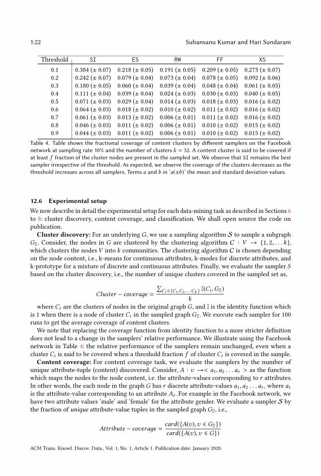
1:22 Suhansanu Kumar and Hari Sundaram
Threshold SI ES RW FF XS
0.1 0.384 (± 0.07) 0.218 (± 0.05) 0.191 (± 0.05) 0.209 (± 0.05) 0.273 (± 0.07)
0.2 0.242 (± 0.07) 0.079 (± 0.04) 0.073 (± 0.04) 0.078 (± 0.05) 0.092 (± 0.06)
0.3 0.180 (± 0.05) 0.060 (± 0.04) 0.039 (± 0.04) 0.048 (± 0.04) 0.061 (± 0.05)
0.4 0.111 (± 0.04) 0.039 (± 0.04) 0.024 (± 0.03) 0.030 (± 0.03) 0.040 (± 0.05)
0.5 0.071 (± 0.03) 0.029 (± 0.04) 0.014 (± 0.03) 0.018 (± 0.03) 0.016 (± 0.02)
0.6 0.064 (± 0.03) 0.018 (± 0.02) 0.010 (± 0.02) 0.011 (± 0.02) 0.016 (± 0.02)
0.7 0.061 (± 0.03) 0.013 (± 0.02) 0.006 (± 0.01) 0.011 (± 0.02) 0.016 (± 0.02)
0.8 0.046 (± 0.03) 0.011 (± 0.02) 0.006 (± 0.01) 0.010 (± 0.02) 0.015 (± 0.02)
0.9 0.044 (± 0.03) 0.011 (± 0.02) 0.006 (± 0.01) 0.010 (± 0.02) 0.015 (± 0.02)
Table 4. Table shows the fractional coverage of content clusters by different samplers on the Facebooknetwork at sampling rate 10% and the number of clusters k = 32. A content cluster is said to be covered ifat least f fraction of the cluster nodes are present in the sampled set. We observe that SI remains the bestsampler irrespective of the threshold. As expected, we observe the coverage of the clusters decreases as thethreshold increases across all samplers. Terms a and b in ‘a(±b)’ the mean and standard deviation values.
12.6 Experimental setupWenow describe in detail the experimental setup for each data-mining task as described in Sections 6
to 8: cluster discovery, content coverage, and classification. We shall open source the code on
publication.
Cluster discovery: For an underlying G, we use a sampling algorithm S to sample a subgraph
GS. Consider, the nodes in G are clustered by the clustering algorithm C : V → {1, 2, . . .k},which clusters the nodes V into k communities. The clustering algorithm C is chosen depending
on the node content, i.e., k-means for continuous attributes, k-modes for discrete attributes, and
k-prototype for a mixture of discrete and continuous attributes. Finally, we evaluate the sampler Sbased on the cluster discovery, i.e., the number of unique clusters covered in the sampled set as,
Cluster − coveraдe =
∑Ci ∈{C1,C2, ...Ck } I(Ci ,GS)
kwhere Ci are the clusters of nodes in the original graph G, and I is the identity function which
is 1 when there is a node of cluster Ci in the sampled graph GS. We execute each sampler for 100
runs to get the average coverage of content clusters.
We note that replacing the coverage function from identity function to a more stricter definition
does not lead to a change in the samplers’ relative performance. We illustrate using the Facebook
network in Table 4: the relative performance of the samplers remain unchanged, even when a
cluster Ci is said to be covered when a threshold fraction f of cluster Ci is covered in the sample.
Content coverage: For content coverage task, we evaluate the samplers by the number of
unique attribute-tuple (content) discovered. Consider, A : v →< a1,a2 . . . ar > as the function
which maps the nodes to the node content, i.e. the attribute-values corresponding to r attributes.In other words, the each node in the graph G has r discrete attribute-values a1,a2 . . . ar , where aiis the attribute-value corresponding to an attribute Ai . For example in the Facebook network, we
have two attribute values ‘male‘ and ‘female‘ for the attribute gender. We evaluate a sampler S by
the fraction of unique attribute-value tuples in the sampled graph GS, i.e.,
Attribute − coveraдe =card({A(v),v ∈ GS})
card({A(v),v ∈ G})
ACM Trans. Knowl. Discov. Data., Vol. 1, No. 1, Article 1. Publication date: January 2020.

Attribute-guided network sampling mechanisms 1:23
where card(·) is the cardinality of a set. Thus, a sampler sampling most nodes with unique
attribute-tuples (content) will have higher attribute coverage.
Classification & Regression: For each run of the classification and regression task, we ran-
domly split the nodes of the graph G into the test and train set with a split-ratio of 20%-80%.
Next, we mask the test nodes so that no sampler can use the test nodes for training the classifier.
Thereafter, we train a classifier f : A(v) → y that takes the unmasked sampled nodes’ attributes as
input and the node label as the output. The above procedure ensures that the training and testing
set is the same for all the samplers. The sampling policy determines which subset of nodes to
sample from unmasked node-set. The sampler stops when the number of unmasked nodes sampled
reaches the sampling budget. We use the sklearn implementation of the SVM classifier with default
parameters4for training and testing the node labels. We observe similar relative performance
of the samplers when using other classification algorithms like Random Forest and Naive Bayes
classifier.
REFERENCES[1] Nesreen K Ahmed, Jennifer Neville, and Ramana Kompella. 2013. Network sampling: From static to streaming graphs.
ACM Transactions on Knowledge Discovery from Data (TKDD) 8, 2 (2013), 1–56.[2] Yong-Yeol Ahn, James P Bagrow, and Sune Lehmann. 2010. Link communities reveal multiscale complexity in networks.
Nature 466, 7307 (2010), 761–764.[3] Alberto Apostolico and Guido Drovandi. 2009. Graph compression by BFS. Algorithms 2, 3 (2009), 1031–1044.[4] Mansurul A Bhuiyan, Mahmudur Rahman, Mahmuda Rahman, and Mohammad Al Hasan. 2012. Guise: Uniform
sampling of graphlets for large graph analysis. In 2012 IEEE 12th International Conference on Data Mining. IEEE, 91–100.[5] Soumen Chakrabarti, Martin Van den Berg, and Byron Dom. 1999. Focused crawling: a new approach to topic-specific
Web resource discovery. Computer networks 31, 11-16 (1999), 1623–1640.[6] Flavio Chiericetti, Anirban Dasgupta, Ravi Kumar, Silvio Lattanzi, and Tamas Sarlos. 2016. On sampling nodes in
a network. In Proceedings of the 25th International Conference on World Wide Web. International World Wide Web
Conferences Steering Committee, 471–481.
[7] Elizabeth Costenbader and Thomas W Valente. 2003. The stability of centrality measures when networks are sampled.
Social networks 25, 4 (2003), 283–307.[8] Gabor Csardi and Tamas Nepusz. 2006. The igraph software package for complex network research. InterJournal,
Complex Systems 1695, 5 (2006), 1–9.[9] Tomás Feder and Rajeev Motwani. 1995. Clique partitions, graph compression and speeding-up algorithms. J. Comput.
System Sci. 51, 2 (1995), 261–272.[10] Santo Fortunato and Darko Hric. 2016. Community detection in networks: A user guide. Physics reports 659 (2016),
1–44.
[11] Mina Ghavipour and Mohammad Reza Meybodi. 2017. Irregular cellular learning automata-based algorithm for
sampling social networks. Engineering Applications of Artificial Intelligence 59 (2017), 244–259.[12] M. Gjoka, M. Kurant, C.T. Butts, and A. Markopoulou. 2010. Walking in Facebook: A Case Study of Unbiased Sampling
of OSNs. In INFOCOM, 2010 Proceedings IEEE. 1–9.[13] Minas Gjoka, Maciej Kurant, Carter T Butts, and Athina Markopoulou. 2009. A walk in facebook: Uniform sampling of
users in online social networks. arXiv preprint arXiv:0906.0060 (2009).[14] Minas Gjoka, Emily Smith, and Carter T Butts. 2015. Estimating subgraph frequencies with or without attributes from
egocentrically sampled data. arXiv preprint arXiv:1510.08119 (2015).[15] Jerzy W Grzymala-Busse and Ming Hu. 2000. A comparison of several approaches to missing attribute values in data
mining. In International Conference on Rough Sets and Current Trends in Computing. Springer, 378–385.[16] Douglas D Heckathorn. 1997. Respondent-driven sampling: a new approach to the study of hidden populations.
SOCIAL PROBLEMS-NEW YORK- 44 (1997), 174–199.[17] Cesar A Hidalgo and Carlos Rodriguez-Sickert. 2008. The dynamics of a mobile phone network. Physica A: Statistical
Mechanics and its Applications 387, 12 (2008), 3017–3024.[18] Pili Hu and Wing Cheong Lau. 2013. A survey and taxonomy of graph sampling. arXiv preprint arXiv:1308.5865 (2013).[19] Zhexue Huang. 1997. Clustering large data sets with mixed numeric and categorical values. In Proceedings of the 1st
pacific-asia conference on knowledge discovery and data mining,(PAKDD). Singapore, 21–34.
4https://scikit-learn.org/stable/modules/generated/sklearn.svm.SVC.html
ACM Trans. Knowl. Discov. Data., Vol. 1, No. 1, Article 1. Publication date: January 2020.

1:24 Suhansanu Kumar and Hari Sundaram
[20] Christian Hubler, Hans-Peter Kriegel, Karsten Borgwardt, and Zoubin Ghahramani. 2008a. Metropolis algorithms
for representative subgraph sampling. In Data Mining, 2008. ICDM’08. Eighth IEEE International Conference on. IEEE,283–292.
[21] C. Hubler, H.-P. Kriegel, K. Borgwardt, and Z. Ghahramani. 2008b. Metropolis Algorithms for Representative Subgraph
Sampling. In Data Mining, 2008. ICDM ’08. Eighth IEEE International Conference on. 283–292.[22] David Kempe, Jon Kleinberg, and Eva Tardos. 2003. Maximizing the Spread of Influence Through a Social Network. In
Proceedings of the Ninth ACM SIGKDD International Conference on Knowledge Discovery and Data Mining (KDD ’03).ACM, New York, NY, USA, 137–146. DOI:http://dx.doi.org/10.1145/956750.956769
[23] Maciej Kurant, Athina Markopoulou, and Patrick Thiran. 2010. On the bias of bfs (breadth first search). In TeletrafficCongress (ITC), 2010 22nd International. IEEE, 1–8.
[24] Andrea Lancichinetti and Santo Fortunato. 2009. Benchmarks for testing community detection algorithms on directed
and weighted graphs with overlapping communities. Physical Review E 80, 1 (2009), 016118.
[25] Doris Jung-Lin Lee, Jinda Han, Dana Chambourova, and Ranjitha Kumar. 2017. Identifying Fashion Accounts in Social
Networks. In KDD Workshop on ML Meets Fashion.[26] Jure Leskovec and Christos Faloutsos. 2006. Sampling from large graphs. In Proceedings of the 12th ACM SIGKDD
international conference on Knowledge discovery and data mining. ACM, 631–636.
[27] Jure Leskovec, Jon Kleinberg, and Christos Faloutsos. 2005. Graphs over time: densification laws, shrinking diameters
and possible explanations. In Proceedings of the eleventh ACM SIGKDD international conference on Knowledge discoveryin data mining. ACM, 177–187.
[28] Jure Leskovec, Andreas Krause, Carlos Guestrin, Christos Faloutsos, Jeanne VanBriesen, and Natalie Glance. 2007.
Cost-effective outbreak detection in networks. In Proceedings of the 13th ACM SIGKDD international conference onKnowledge discovery and data mining. ACM, 420–429.
[29] Jure Leskovec, Kevin J Lang, Anirban Dasgupta, and Michael W Mahoney. 2009. Community structure in large
networks: Natural cluster sizes and the absence of large well-defined clusters. Internet Mathematics 6, 1 (2009), 29–123.[30] Jhao-Yin Li and Mi-Yen Yeh. 2011. On sampling type distribution from heterogeneous social networks. In Advances in
Knowledge Discovery and Data Mining. Springer, 111–122.[31] Arun S Maiya and Tanya Y Berger-Wolf. 2011. Benefits of bias: Towards better characterization of network sampling. In
Proceedings of the 17th ACM SIGKDD international conference on Knowledge discovery and data mining. ACM, 105–113.
[32] Julian J McAuley and Jure Leskovec. 2012. Learning to Discover Social Circles in Ego Networks.. In NIPS, Vol. 2012.548–56.
[33] Fabricio Murai, Diogo Rennó, Bruno Ribeiro, Gisele L Pappa, Don Towsley, and Krista Gile. 2018. Selective harvesting
over networks. Data Mining and Knowledge Discovery 32, 1 (2018), 187–217.
[34] Yohsuke Murase, Hang-Hyun Jo, János Török, János Kertész, and Kimmo Kaski. 2019. Sampling networks by nodal
attributes. Physical Review E 99, 5 (2019), 052304.
[35] George L Nemhauser, Laurence A Wolsey, and Marshall L Fisher. 1978. An analysis of approximations for maximizing
submodular set functions—I. Mathematical Programming 14, 1 (1978), 265–294.
[36] Mark EJ Newman. 2003. Mixing patterns in networks. Physical Review E 67, 2 (2003), 026126.
[37] Hosung Park and Sue Moon. 2013. Sampling bias in user attribute estimation of OSNs. In Proceedings of the 22ndinternational conference onWorldWideWeb companion. InternationalWorldWideWeb Conferences Steering Committee,
183–184.
[38] Michael Quinn Patton. 2005. Qualitative research. Wiley Online Library.
[39] Fernando Perez-Cruz. 2008. Kullback-Leibler divergence estimation of continuous distributions. In Information Theory,2008. ISIT 2008. IEEE International Symposium on. IEEE, 1666–1670.
[40] Joseph J Pfeiffer III, Sebastian Moreno, Timothy La Fond, Jennifer Neville, and Brian Gallagher. 2014. Attributed graph
models: Modeling network structure with correlated attributes. In Proceedings of the 23rd international conference onWorld wide web. 831–842.
[41] Joseph J Pfeiffer III, Jennifer Neville, and Paul N Bennett. 2013. Combining Active Sampling with Parameter Estimation
and Prediction in Single Networks. In Proceedings of the ICML Structured Learning Workshop.[42] Robert Pienta, Zhiyuan Lin, Minsuk Kahng, Jilles Vreeken, Partha P Talukdar, James Abello, Ganesh Parameswaran,
and Duen Horng Polo Chau. 2015. AdaptiveNav: Discovering Locally Interesting and Surprising Nodes in Large
Graphs. (2015).
[43] Pablo Robles, Sebastian Moreno, and Jennifer Neville. 2016. Sampling of attributed networks from hierarchical
generative models. In Proceedings of the 22nd ACM SIGKDD International Conference on Knowledge Discovery and DataMining. 1155–1164.
[44] Sunita Sarawagi. 2000. User-Adaptive Exploration of Multidimensional Data.. In VLDB. 307–316.[45] Daniel A Spielman and Nikhil Srivastava. 2011. Graph sparsification by effective resistances. SIAM J. Comput. 40, 6
(2011), 1913–1926.
ACM Trans. Knowl. Discov. Data., Vol. 1, No. 1, Article 1. Publication date: January 2020.

Attribute-guided network sampling mechanisms 1:25
[46] Lubos Takac and Michal Zabovsky. 2012. Data analysis in public social networks. International Scientific Conferenceand International Workshop Present Day Trends of Innovations 1 (2012).
[47] Claudia Wagner, Philipp Singer, Fariba Karimi, Jurgen Pfeffer, and Markus Strohmaier. 2017. Sampling from Social
Networks with Attributes. In Proceedings of the 26th International Conference on World Wide Web. International World
Wide Web Conferences Steering Committee, 1181–1190.
[48] Qing Wang, Sanjeev R Kulkarni, and Sergio Verdu. 2006. A nearest-neighbor approach to estimating divergence
between continuous random vectors. In Information Theory, 2006 IEEE International Symposium on. IEEE, 242–246.[49] Cheng-Lun Yang, Perng-Hwa Kung, Cheng-Te Li, Chun-An Chen, and Shou-De Lin. 2013a. Sampling Heterogeneous
Networks. In Data Mining (ICDM), 2013 IEEE 13th International Conference on. IEEE, 1247–1252.[50] Jaewon Yang, Julian McAuley, and Jure Leskovec. 2013b. Community detection in networks with node attributes. In
Data Mining (ICDM), 2013 IEEE 13th international conference on. IEEE, 1151–1156.
ACM Trans. Knowl. Discov. Data., Vol. 1, No. 1, Article 1. Publication date: January 2020.


![Deformable MRI-Ultrasound Registration via Attribute ...you2/publications/Machado... · image-guided neurosurgery based on neuronavigation systems [1–3]. Intraoperative ultrasound,](https://img.dokumen.tips/doc/110x75/5fd9eec69cfe577ae9403ac8/deformable-mri-ultrasound-registration-via-attribute-you2publicationsmachado.jpg)