Embed Size (px)
Citation preview

LETTER Communicated by Morris Hirsch
Attractive Periodic Sets in Discrete-Time Recurrent Networks(with Emphasis on Fixed-Point Stability and Bifurcations inTwo-Neuron Networks)
Peter Ti IumlnoAston University Birmingham B4 7ET UK and Department of Computer Scienceand Engineering Slovak University of Technology 812 19 Bratislava Slovakia
Bill G HorneNEC Research Institute Princeton NJ 08540 USA
C Lee GilesNEC Research Institute Princeton NJ 08540 USA and School of Information Sci-ences and Technology Pennsylvania State University University Park PA 16801USA
We perform a detailed xed-point analysis of two-unit recurrent neuralnetworks with sigmoid-shaped transfer functions Using geometrical ar-guments in the space of transfer function derivatives we partition thenetwork state-space into distinct regions corresponding to stability typesof the xed points Unlike in the previous studies we do not assume anyspecial form of connectivity pattern between the neurons and all freeparameters are allowed to vary We also prove that when both neuronshave excitatory self-connections and the mutual interaction pattern is thesame (ie the neurons mutually inhibit or excite themselves) new attrac-tive xed points are created through the saddle-node bifurcation Finallyfor an N-neuron recurrent network we give lower bounds on the rateof convergence of attractive periodic points toward the saturation val-ues of neuron activations as the absolute values of connection weightsgrow
1 Introduction
Discrete-time recurrent neural networks offer a wide range of dynamical be-havior They can generate steady-state periodic quasi-periodic and chaoticorbits
Attractive xed points have been proposed as robust representations ofprototype vectors in associative memories (Amit 1989 Hopeld 1984 Huiamp Zak 1992) Indeed a great deal of work has focused on the question ofhow to constrain the weights in the recurrent network so that it exhibits onlyattractive steady states (Casey 1995 Jin Nikiforuk amp Gupta 1994 Sevrani
Neural Computation 13 1379ndash1414 (2001) cdeg 2001 Massachusetts Institute of Technology
1380 Peter Ti Iumlno Bill G Horne and C Lee Giles
amp Abe 2000) Jin et al (1994) give the conditions on the weight matrix underwhich all xed points of the network are attractive
Saddle xed points were suggested to play an important role in workingmemories operating in nonstationary environments where both long-termmaintenance and quick transitions are desirable (McAuley amp Stampi 1994Nakahara amp Doya 1998) Moreover saddle points often mimicstack-like be-havior in recurrent networks trained on context-free languages (RodriguezWiles amp Elman 1999) Also they were found to be part of a mechanism bywhich recurrent networks induce nonstable representations of large cyclesin nite state machines (Ti Iumlno Horne Giles amp Collingwood 1998)
There are many applications where oscillatory dynamics of recurrentnetworks is desirable For example when trained to act as a nite statemachine (Cleeremans Servan-Schreiber amp McClelland 1989 Giles et al1992 Ti Iumlno amp Sajda 1995 Watrous amp Kuhn 1992) the network has to inducea stable representation of state transitions associated with each input symbols of the machine Of special importance are period-n cycles driven by sgiven the current state S when repeatedly presenting the input s we returnafter n steps to SCycles in the machine often induce in the recurrentnetworkstate-space stable periodic orbits corresponding to the input s (Casey 1996Manolios amp Fanelli 1994 Ti Iumlno et al 1998) In particular loops that isperiod 1 cycles often induce attractive xed points (see eg Casey 1996Ti Iumlno et al 1998)
Finally chaotic behavior of recurrent networks has been a focus of a vividresearch activity (Botelho 1999 Klotz amp Brauer 1999 Pasemann 1995a)especially after Wang (1991) rigorously showed that a simple two-neuronrecurrent network is capable of producing chaos
There is a considerable amount of literature on two-unit recurrent net-works (Beer 1995 Borisyuk amp Kirillov 1992 Botelho 1999 Klotz amp Brauer1999Pakdamann Grotta-Ragazzo Malta Arino amp Vibert 1998Pasemann1993 Wang 1991 Zhou 1996) This is partly due to the lack of mathematicaltools for a detailed analysis of higher-dimensional dynamical systems andpartly due to the high expressive power of such simple networks in whichmany generic properties of larger networks are already present (Botelho1999) Moreover two-neuron networks are sometimes thought of as sys-tems of two modules where each module represents the mean activity of aspatially localized neural population (Borisyuk amp Kirillov 1992 Pasemann1995a Tonnelier Meignen Bosh amp Demongeot 1999)
Typically studies of the asymptotic behavior of two-unit or larger net-works assume some form of structure in the weight matrix describing theconnectivity pattern among recurrent neurons We mention a few exam-ples
Symmetric connectivity and absence of self-interactions enabled Hopeld(1984) to interpret the network as a physical system having energyminima in the attractive xed points These rather strict conditions
Attractive Periodic Sets 1381
were weakened in Casey (1995) Blum and Wang (1992) globally ana-lyzed networks with nonsymmetrical connectivity patterns of specialtypes In particular they formulated results for two-neuron networkswith the logistic sigmoid transfer function g( ) D 1 (1 C eiexcl`) in theabsence of neuron self-connections
Deep mathematical studies were presented for severely restricted top-ologies such as the ldquoring networkrdquo (Pasemann 1995b) or the chainoscillators (Wang 1996)
Often rather detailed bifurcation studies are performed with respectto only one or two network parameters the remaining parameters arekept xed to ldquoappropriaterdquo values (Borisyuk amp Kirillov 1992 Naka-hara amp Doya 1998)
Also the assumption of saturated sigmoidal or linear transfer functions(as in the Brain-State-in-a-Box model Anderson 1993) makes the study ofasymptotically stable equilibrium points more feasible (Botelho 1999 Huiamp Zak 1992 Sevrani amp Abe 2000)
In this article we impose no conditions on connection weights or externalinputs apart from the fact that the weights are assumed to be nonzero Toour knowledge a thorough xed-pointanalysis of two-unit neural networkswith sigmoid transfer functions is still missing1 We offer such an analysis insections 4 and 5 In section 6 we rigorously explain the mechanism by whichnew attractive xed points are createdmdashthe saddle-node bifurcation Thisconrms the empirical ndings of Tonnelier et al (1999) When studyingsuch networks they empirically observed that a new xed point appearsthrough the saddle-node bifurcation
Hirsch (1994) proved that when all the weights in an N-neuron recur-rent network with exclusively self-exciting (or exclusively self-inhibiting)neurons are multiplied by an increasing neural gain attractive xed pointstend toward the saturated activation values In section 7 we give a lowerbound on the rate of convergence of attractive periodic points2 toward thesaturation values The results hold for ldquosigmoid-shapedrdquo neuron transferfunctions This investigation was motivated by the observation of many inthe recurrent network grammarautomata induction community that theactivations of recurrent neurons often cluster away from the center of thenetwork state-space and close to the saturated activation values (eg Mano-lios amp Fanelli 1994 Ti Iumlno et al 1998) In fact this was exploited by ZengGoodman and Smyth (1993) in a heuristic to stabilize the induced automatarepresentations in the recurrent network
1 The most complete xed-point analysis of continuous-time two-neuron networks canbe found in Beer (1995)We determine the xed-point positions using a similar ldquonull-clinerdquotechnique
2 Fixed points can be considered periodic points of period 1
1382 Peter Ti Iumlno Bill G Horne and C Lee Giles
In the next two sections we recall some basic concepts from the theory ofdynamical systems and introduce the recurrent network model
2 Basic Denitions
A discrete-time dynamical system can be represented as the iteration of a(differentiable) map f X X X microltd
xnC1 D f (xn) n 2 N (21)
Here N denotes the set of all natural numbers For each x D x0 2 X theiteration 21 generates a sequence of points dening the orbit or trajectoryof x under the map f In other words the orbit of x under f is the sequencef f n(x)gncedil0 For n cedil 1 f n is the composition of the map f with itself n timesf 0 is dened to be the identity map on X
A point x 2 X is called a xed point of the map f if f (x) D x It is calleda periodic point of period P if it is a xed point of f P
Fixed points can be classied according to the orbit behavior of pointsin their vicinity A xed point x is said to be asymptotically stable (or anattractive point of f ) if there exists a neighborhood O(x) of x such thatlimn1 f n(y) D x for all y 2 O(x) As n increases trajectories of points nearan asymptotically stable xed point tend toward it
A xed point x of f is asymptotically stable only if for each eigenvalue lof J (x) the Jacobian of f at x |l| lt 1 holds The eigenvalues of the JacobianJ (x) govern the contracting and expanding directions of the map f in avicinity of x Eigenvalues larger in absolute value than 1 lead to expansionswhereas eigenvalues smaller than 1 correspond to contractions If all theeigenvalues of J (x) are outside the unit circle x is a repulsive point As thetime index n increases the trajectories of points from a neighborhood of arepulsive point move away from it If some eigenvalues of J (x) are insideand some are outside the unit circle x is said to be a saddle point
3 The Model
In this article we study recurrent neural networks with transfer functionsfrom a general class of ldquosigmoid-shapedrdquo maps
gABm ( ) DA
1 C eiexclm `C B (31)
transforming lt into the interval (B B C A) B 2 lt A 2 (0 1) The so-calledneural gain m gt 0 controls the ldquosteepnessrdquo of the transfer function Asm 1 gABm tends to the step function gABm ( ) D B for ` lt 0 andgABm ( ) D B C A for ` cedil 0 The commonly used unipolar and bipolar lo-gistic transfer functions can be expressed as g101 and g2iexcl11 respectively
Attractive Periodic Sets 1383
21
w
w12
21
w w
T1 T
2
11 22
Figure 1 A two-dimensional recurrent neural network
Another commonly used transfer function the hyperbolic tangent corre-sponds to g2iexcl12
For recurrent networks consisting of two neurons (see Figure 1) the it-erative map equation 21 can be written as follows
microxnC1ynC1
paraD
microgABm (w11xn C w12yn C T1)gABm (w21xn C w22yn C T2)
para (32)
The neuron outputs (activations) (xn yn) 2 (B B C A)2 form the state of thenetworkat time step n The connection weights wij 2 ltnf0g and biasexternalinput terms Ti 2 lt are the adjustable parameters of the network and deter-mine the dynamical behavior of the system 32
For the purpose of xed-point analysis of equation 32 it is convenientto include the neural gain m into the adjustable parameters We rewriteequation 32 as
microxnC1ynC1
paraD
microg(axn C byn C t1)g(cxn C dyn C t2)
para (33)
where g D gAB1 a D m w11 b D m w12 c D m w21 d D m w22 t1 D m T1 andt2 D m T2
4 Analysis in the Space of Transfer Function Derivatives
In this section we work with the derivatives
G1(x y) D g0 ( )| DaxCbyCt1 D g0 (ax C by C t1) (41)
G2(x y) D g0 ( )|`DcxCdyCt2 D g0 (cx C dy C t2) (42)
of transfer functions corresponding to the two neurons in the network de-scribed by equation 33 The derivatives G1 and G2 are always positive Ouraim is to partition the space of derivatives (G1 G2) 2 (0 A
4 )2 into regionscorresponding to stability types of the neural network xed points
1384 Peter Ti Iumlno Bill G Horne and C Lee Giles
First we introduce two auxiliary maps y (B B C A) (0 A4]
y (u) D1A
(u iexcl B)(B C A iexcl u) (43)
and w (B B C A)2 (0 A4]2
w (x y) D (y (x) y (y)) (44)
It is easy to show that
g0 ( ) D1A
(g( ) iexcl B)(B C A iexcl g( )) D y (g( )) (45)
For each xed point (x y) of equation 33
microxy
paraD
microg(ax C by C t1)g(cx C dy C t2)
para (46)
and so by equations 41 42 45 and 46
G1(x y) D y (g(ax C by C t1)) D y (x) (47)
G2(x y) D y (g(cx C dy C t2)) D y (y) (48)
which implies (see equation 44)
(G1(x y) G2(x y)) D w (x y) (49)
Consider a function F(u v) F A micro lt2 lt The function F induces apartition of the set A into three regions
Fiexcl D f(u v) 2 A|F(u v) lt 0g (410)
FC D f(u v) 2 A|F(u v) gt 0g (411)
F0 D f(u v) 2 A|F(u v) D 0g (412)
Now we are ready to formulate and prove three lemmas that dene thecorrespondence between the derivatives G1 and G2 of the neuron transferfunctions (see equations 41 and 42) and the xed-point stability of thenetwork equation 33
Lemma 1 If bc gt 0 then all attractive xed points (x y) of equation 33 satisfy
w (x y) 2sup3
01|a|
acutepound
sup30
1|d|
acute
Attractive Periodic Sets 1385
Proof Consider a xed point (x y) of equation 33 By equations 41 and 42the Jacobian J (x y) of equation 33 in (x y) is given by3
J Dsup3
aG1(x y) bG1(x y)cG2(x y) dG2(x y)
acute
The eigenvalues of J are
l12 DaG1 C dG2 sect
pD(G1 G2)
2 (413)
where
D(G1 G2) D (aG1 iexcl dG2)2 C 4G1G2bc (414)
The proof continues with an analysis of three separate cases correspond-ing to sign patterns of weights associated with the neuron self-connections
In the rst case assume a d gt 0 that is the weights of self-connectionson both neurons are positive Dene
a(G1 G2) D aG1 C dG2 (415)
Since the derivatives G1 G2 can only take on values from (0 A4) anda d gt 0 we have D(G1 G2) gt 0 and a(G1 G2) gt 0 for all (G1 G2) 2(0 A4)2 Inour terminology(see equations 410ndash412) DC aC D (0 A4)2 micro(0 1)2 To identify possible values of G1 and G2 so that |l12 | lt 1 it is suf-cient to solve the inequality aG1 C dG2 C
pD(G1 G2) lt 2 or equivalently
2 iexcl aG1 iexcl dG2 gtp
D(G1 G2) (416)
Consider only (G1 G2) such that
r1(G1 G2) D aG1 C dG2 iexcl 2 lt 0 (417)
that is (G1 G2) lying under the line r 01 aG1 C dG2 D 2 All (G1 G2) such
that aG1 C dG2 iexcl 2 gt 0 that is (G1 G2) 2 r C1 (above r 0
1 ) lead to at leastone eigenvalue of J greater in absolute value than 1 Squaring both sidesof equation 416 we arrive at
k1(G1 G2) D (ad iexcl bc)G1G2 iexcl aG1 iexcl dG2 C 1 gt 0 (418)
3 To simplify the notation the identication (x y) of the xed point in which equa-tion 33 is linearized is omitted
1386 Peter Ti Iumlno Bill G Horne and C Lee Giles
k10
G2
1a
1d
k10
G1
k10
~
ad=bc
adgtbc1d
1a
10r
~
(00)
adltbc
Figure 2 Illustration for the proof of lemma 1 The network parameters satisfya d gt 0 and bc gt 0 All (G1 G2 ) 2 (0 A4]2 below the left branch of k 0
1 (ifad cedil bc) or between the branches ofk 0
1 (if ad lt bc) correspond to the attractivexed points Different line styles for k 0
1 are associated with the cases ad gt bcad D bc and ad lt bcmdashthe solid dashed-dotted and dashed lines respectively
If ad 6D bc the set k 01 is a hyperbola
G2 D1Qd
CC
G1 iexcl 1Qa
(419)
with
Qa D a iexcl bcd
(420)
Qd D d iexcl bca
(421)
C Dbc
(ad iexcl bc)2 (422)
It is easy to check that the points (1a 0) and (0 1d) lie on the curvek 01
If ad D bc the set k 01 is a line passing through the points (0 1d) and
(1a 0) (see Figure 2) To summarize when a d gt 0 by equations 49 417and 418 the xed point (x y) of equation 33 is attractive only if
(G1 G2) D w (x y) 2 k C1 riexcl
1
where the map w is dened by equation 44
Attractive Periodic Sets 1387
A necessary (not sufcient) condition for (x y) to be attractive reads4
w (x y) 2sup3
01a
acutepound
sup30
1d
acute
Consider now the case of negative weights on neuron self-connectionsa d lt 0 Since in this case a(G1 G2) (see equation 415) is negative for allvalues of the transfer function derivatives G1 G2 we have aiexcl D (0 A4)2 micro(0 1)2 In order to identify possible values of (G1 G2) such that |l12 | lt 1it is sufcient to solve the inequality aG1 C dG2 iexcl
pD(G1 G2) gt iexcl2 or
equivalently
2 C aG1 C dG2 gtp
D(G1 G2) (423)
As in the previous case we shall consider only (G1 G2) such that
r2(G1 G2) D aG1 C dG2 C 2 gt 0 (424)
since all (G1 G2) 2 riexcl2 lead to at least one eigenvalue of J greater in absolute
value than 1Squaring both sides of equation 423 we arrive at
k2(G1 G2) D (ad iexcl bc)G1G2 C aG1 C dG2 C 1 gt 0 (425)
which is equivalent to
((iexcla)(iexcld) iexcl bc)G1G2 iexcl (iexcla)G1 iexcl (iexcld)G2 C 1 gt 0 (426)
Further analysis is exactly the same as the analysis from the previous case(a d gt 0) with a Qa d and Qd replaced by |a| |a| iexcl bc |d| |d| and |d| iexcl bc |a|respectively
If ad 6D bc the set k 02 is a hyperbola
G2 Diexcl1
QdC
C
G1 C 1Qa
(427)
passing through the points (iexcl1a 0) and (0 iexcl1d)
4 If ad gt bc then 0 lt Qa lt a and 0 lt Qd lt d (see equations 420 and 421) Thederivatives (G1 G2 ) 2 k C
1 lie under the ldquoleft branchrdquo and above the ldquoright branchrdquo ofk 0
1 (see Figure 2) It is easy to see that since we are conned to the half-plane riexcl1 (below
the line r 01 ) only (G1 G2 ) under the ldquoleft branchrdquo of k 0
1 will be considered Indeed r 01 is
a decreasing line going through the point (1a 1d) and so it never intersects the rightbranch of k 0
1 If ad lt bc then Qa Qd lt 0 and (G1 G2) 2 k C1 lie between the two branches
of k 01
1388 Peter Ti Iumlno Bill G Horne and C Lee Giles
If ad D bck 02 is the line dened by the points (0 iexcl1d) and (iexcl1a 0)
By equations 49 424 and 425 the xed point (x y) of equation 33 isattractive only if
(G1 G2) D w (x y) 2 k C2 r C
2
In this case the derivatives (G1 G2) D w (x y) must satisfy
w (x y) 2sup3
01|a|
acutepound
sup30
1|d|
acute
Finally consider the case when the weights on neuron self-connectionsdiffer in sign Without loss of generality assume a gt 0 and d lt 0 Assumefurther that aG1 C dG2 cedil 0 that is (G1 G2) 2 aC [ a0 (see equation 415) lieunder or on the line
a0 G2 Da
|d|G1
It is sufcient to solve inequality 416 Using equations 417 and 418 andarguments developed earlier in this proof we conclude that the derivatives(G1 G2) lying in
k C1 riexcl
1 (aC [ a0)
correspond to attractive xed points of equation 33 (see Figure 3) Sincea gt 0 and d lt 0 the term ad iexcl bc is negative and so 0 lt a lt Qa Qd lt d lt 0The ldquotransformedrdquo parameters Qa Qd are dened in equations 420 and 421For (G1 G2) 2 aiexcl by equations 424 and 425 and earlier arguments in thisproof the derivatives (G1 G2) lying in
k C2 r C
2 aiexcl
correspond to attractive xed points of equation 33It can be easily shown that the sets k 0
1 and k 02 intersect on the line a0 in
the open interval (see Figure 3)
sup31Qa
1a
acutepound
sup31
| Qd|
1|d|
acute
We conclude that the xed point (x y) of equation 33 is attractive only if
w (x y) 2 [k C1 riexcl
1 (aC [ a0)] [ [k C2 r C
2 aiexcl]
In particular if (x y) is attractive then the derivatives (G1 G2) D w (x y)must lie in
sup30
1a
acutepound
sup30
1|d|
acute
Attractive Periodic Sets 1389
G1
G2
k10
k10
k02
-1d~
-1a~ 1a~
10r
k02
1d
-1d
-1a1a
0r2
(00)
1d~
0a
Figure 3 Illustration for the proof of lemma 1 The network parameters areconstrained as follows a gt 0 d lt 0 and bc gt 0 All (G1 G2) 2 (0 A4]2 belowand on the line a0 and between the two branches ofk 0
1 (solid line) correspond tothe attractive xed points So do all (G1 G2 ) 2 (0 A4]2 above a0 and betweenthe two branches ofk 0
2 (dashed line)
Examination of the case a lt 0 d gt 0 in the same way leads to a conclu-sion that all attractive xed points of equation 33 have their correspondingderivatives (G1 G2) in
sup30
1|a|
acutepound
sup30
1d
acute
We remind the reader that the ldquotransformedrdquo parameters Qa and Qd aredened in equations 420 and 421
Lemma 2 Assume bc lt 0 Suppose ad gt 0 or ad lt 0 with |ad| middot |bc| 2Then each xed point (x y) of equation 33 such that
w (x y) 2sup3
01|a|
acutepound
sup30
1
| Qd|
acute[
sup30
1| Qa|
acutepound
sup30
1|d|
acute
is attractive In particular all xed points (x y) for which
w (x y) 2sup3
01| Qa|
acutepound
sup30
1
| Qd|
acute
are attractive
1390 Peter Ti Iumlno Bill G Horne and C Lee Giles
Proof The discriminant D(G1 G2) in equation 414 is no longer exclusivelypositive It follows from analytic geometry (see eg Anton 1980) thatD(G1 G2) D 0 denes either a single point or two increasing lines (thatcan collide into one or disappear) Furthermore D(0 0) D 0 Hence the setD0 is either a single pointmdashthe originmdashor a pair of increasing lines (thatmay be the same) passing through the origin
As in the proof of the rst lemma we proceed in three stepsFirst assume a d gt 0 Since
Dsup3
1a
1d
acuteD
4bcad
lt 0
and
Dsup3
1a
0acute
D Dsup3
01d
acuteD 1 gt 0
the point (1a 1d) is always in the set Diexcl while (1a 0) (0 1d) 2 DC Weshall examine the case when D(G1 G2) is negative From
|l12 |2 D(aG1 C dG2)2 C |D |
4D G1G2(ad iexcl bc)
it follows that (G1 G2) 2 Diexcl for which |l12 | lt 1 lie in (see Figure 4)
Diexcl giexcl
where
g(G1 G2) D (ad iexcl bc)G1G2 iexcl 1 (428)
It is easy to show that
sup31a
1Qd
acute
sup31Qa
1d
acute2 g0
1Qa
lt1a
1Qd
lt1d
andsup3
1a
1Qd
acute
sup31Qa
1d
acute2 Diexcl
Turn now to the case D(G1 G2) gt 0 Using the technique from the pre-vious proof we conclude that the derivatives (G1 G2) corresponding toattractive xed points of equation 33 lie in
DC riexcl1 k C
1
that is under the line r 01 and between the two branches of k 0
1 (see equa-tions 414 417 and 418) The sets D0 r 0
1 k 01 and g0 intersect in two points
as suggested in Figure 4 To see this note that for points on g0 it holds
G1G2 D1
ad iexcl bc
Attractive Periodic Sets 1391
1a~
1d~
G1
G2
10r
k10
k10
0h
1a 2a
D
D
1d
2d
(00)
D
D
D
0
0
Figure 4 Illustration for the proof of lemma 2 The parameters satisfy a d gt0 and bc lt 0 All (G1 G2) 2 Diexcl and below the right branch of g0 (dashedline) correspond to the attractive xed points So do (G1 G2) 2 (0 A4]2 in DC
between the two branches ofk 01
and for all (G1 G2) 2 D0 g0 we have
(aG1 C dG2)2 D 4 (429)
For G1 G2 gt 0 equation 429 denes the line r 01 Similarly for (G1 G2) in
the sets k 01 and g0 it holds
aG1 C dG2 D 2
which is the denition of the line r 01 The curvesk 0
1 andg0 are monotonicallyincreasing and decreasing respectively and there is exactly one intersectionpoint of the right branch of g0 with each of the two branches ofk 0
1 For (G1 G2) 2 D0
|l12 | DaG1 C dG2
2
and (G1 G2) corresponding to attractive xed points of equation 33 arefrom
D0 riexcl1
1392 Peter Ti Iumlno Bill G Horne and C Lee Giles
In summary when a d gt 0 each xed point (x y) of equation 33 such that
(G1 G2) D w (x y) 2sup3
01a
acutepound
sup30
1Qd
acute[
sup30
1Qa
acutepound
sup30
1d
acute
is attractiveSecond assume a d lt 0 This case is identical to the case a d gt 0
examined above with a Qa d Qd riexcl1 and k C
1 replaced by |a| | Qa| |d| | Qd| r C2
and k C2 respectively First note that the set D0 is the same as before since
(aG1 iexcl dG2)2 D (|a|G1 iexcl |d|G2)2
Furthermore adiexclbc D |a| |d|iexclbc and so (G1 G2) 2 Diexcl for which |l12 | lt 1lie in
Diexcl giexcl
Again it directly follows thatsup3
1|a|
1
| Qd|
acute
sup31| Qa|
1|d|
acute2 g0
1| Qa|
lt1|a|
1
| Qd|lt
1|d|
and sup31|a|
1
| Qd|
acute
sup31| Qa|
1|d|
acute2 Diexcl
For DC the derivatives (G1 G2) corresponding to attractive xed pointsof equation 33 lie in
DC r C2 k C
2
All (G1 G2) 2 D0 r C2 lead to |l12 | lt 1 Hence when a d lt 0 every xed
point (x y) of equation 33 such that
w (x y) 2sup3
01|a|
acutepound
sup30
1
| Qd|
acute[
sup30
1| Qa|
acutepound
sup30
1|d|
acute
is attractiveFinally consider the case a gt 0 d lt 0 (The case a lt 0 d gt 0 would be
treated in exactly the same way) Assume that Diexcl is a nonempty regionThen ad gt bc must hold and
sup31a
1|d|
acute2 Diexcl
This can be easily seen since for ad lt bc we would have for all (G1 G2)
D(G1G2) D (aG1 iexcl dG2)2 C 4G1G2bc D (aG1 C dG2)2 C 4G1G2(bc iexcl ad) cedil 0
Attractive Periodic Sets 1393
The sign of
Dsup3
1a
1|d|
acuteD 4
sup31 C
bca|d|
acute
is equal to the sign of a|d| C bc D bc iexcl ad lt 0 The derivatives (G1 G2) 2 Diexclfor which |l12 | lt 1 lie in
Diexcl giexcl
Alsosup3
1a
1Qd
acute
sup31| Qa|
1|d|
acute2 g0
Note that Qd cedil |d| and | Qa| cedil a only if 2a|d| middot |bc| Only those (G1 G2) 2 D0 are taken into account forwhich |aG1 CdG2 | lt 2
This is true for all (G1 G2) in
D0 riexcl1 r C
2
If D(G1 G2) gt 0 the inequalities to be solved depend on the sign ofaG1 C dG2 Following the same reasoning as in the proof of lemma 1 we con-clude that the derivatives (G1 G2) corresponding to attractive xed pointsof equation 33 lie in
DC [plusmn[k C
1 riexcl1 (aC [ a0)] [ [k C
2 r C2 aiexcl]
sup2
We saw in the proof of lemma 1 that if a gt 0 d lt 0 and bc gt 0 thenall (G1 G2) 2 (0 1 Qa) pound (0 1 | Qd|) potentially correspond to attractive xedpoints of equation 33 (see Figure 3) In the proof of lemma 2 it was shownthat when a gt 0 d lt 0 bc lt 0 if 2a|d| cedil |bc| then (1a 1 |d| ) is on or underthe right branch of g0 and each (G1 G2) 2 (0 1a) pound (0 1 |d| ) potentiallycorresponds to an attractive xed point of equation 33 Hence the followinglemma can be formulated
Lemma 3 If ad lt 0 and bc gt 0 then every xed point (x y) of equation 33such that
w (x y) 2sup3
01| Qa|
acutepound
sup30
1
| Qd|
acute
is attractiveIf ad lt 0 and bc lt 0 with |ad| cedil |bc| 2 then each xed point (x y) of
equation 33 satisfying
w (x y) 2sup3
01|a|
acutepound
sup30
1|d|
acute
is attractive
1394 Peter Ti Iumlno Bill G Horne and C Lee Giles
5 Transforming the Results to the Network State-Space
Lemmas 1 2 and 3 introduce a structure reecting stability types of xedpoints of equation 33 into the space of transfer function derivatives (G1 G2)In this section we transform our results from the (G1 G2)-space into thespace of neural activations (x y)
For u gt 4A dene
D (u) DA2
r1 iexcl
4A
1u
(51)
The interval (0 A4]2 of all transfer function derivatives in the (G1 G2)-plane corresponds to four intervals partitioning the (x y)-space namely
sup3B B C
A2
para2
(52)sup3
B B CA2
parapound
microB C
A2
B C Aacute
(53)micro
B CA2
B C Aacute
poundsup3
B B CA2
para (54)
microB C
A2
B C Aacute2
(55)
Recall that according to equation 49 the transfer function derivatives(G1(x y) G2(x y)) 2 (0 A4]2 in a xed point (x y) 2 (B B C A)2 of equa-tion 33 are equal to w (x y) where the map w is dened in equations 43 and44 Now for each couple (G1 G2) there are four preimages (x y) under themap w
w iexcl1(G1 G2) Draquosup3
B CA2
sect D
sup31
G1
acute B C
A2
sect D
sup31
G2
acuteacutefrac14 (56)
where D (cent) is dened in equation 51Before stating the main results we introduce three types of regions in
the neuron activation space that are of special importance The regions areparameterized by a d gt A4 and correspond to stability types of xedpoints5 of equation 33 (see Figure 5)
RA00(a d) D
sup3B B C
A2
iexcl D (a)acute
poundsup3
B B CA2
iexcl D (d)acute
(57)
RS00(a d) D
iexclB C A
2 iexcl D (a) B C A2
currenpound
iexclB B C A
2 iexcl D (d)cent
[iexclB B C A
2 iexcl D (a)cent
poundiexclB C A
2 iexcl D (d) B C A2
curren
(58)
5 Superscripts A S and R indicate attractive saddle andrepulsive points respectively
Attractive Periodic Sets 1395
B
B+A2
B+A
B+A
B+A2
B+A2+D(d)
B+A2-D(d)
B+A2-D(a) B+A2+D(a)
y
x
R01
AR01
SR11
SR11
A
R11
SR11
RR01
R01
R00
S
R00
AR00
SR10
S R10
A
R10
SR10
RR00
R
S R
Figure 5 Partitioning of the network state-space according to stability types ofthe xed points
RR00(a d) D
sup3B C
A2
iexcl D (a) B CA2
parapound
sup3B C
A2
iexcl D (d) B CA2
para (59)
Having partitioned the interval (B B C A2]2 (see equation 52) of the(x y)-space into the sets RA
00(a d) RS00(a d) and RR
00(a d) we partition theremaining intervals (see equations 53 54 and 55) in the same mannerThe resulting partition of the network state-space (B B C A)2 can be seenin Figure 5 Regions symmetrical to RA
00(a d) RS00(a d) and RR
00(a d) withrespect to the line x D B C A2 are denoted by RA
10(a d) RS10(a d) and
RR10(a d) respectively Similarly RA
01(a d) RS01(a d) and RR
01(a d) denote theregions symmetrical to RA
00(a d) RS00(a d) and RR
00(a d) respectively withrespect to the line y D B C A2 Finally we denote by RA
11(a d) RS11(a d)
and RR11(a d) the regions that are symmetrical to RA
01(a d) RS01(a d) and
RR01(a d) with respect to the line x D B C A2
We are now ready to translate the results formulated in lemmas 1 2 and3 into the (x y)-space of neural activations
Theorem 1 If bc gt 0 |a| gt 4A and |d| gt 4A then all attractive xed pointsof equation 53 lie in
[
i2IRA
i (|a| |d| )
where I is the index set I D f00 10 01 11g
1396 Peter Ti Iumlno Bill G Horne and C Lee Giles
Theorem 2 If bc lt 0 ad lt 0 |a| gt 4A |d| gt 4A and |ad| cedil |bc| 2 thenall xed points of equation 33 lying in
[
i2IRA
i (|a| |d|) I D f00 10 01 11g
are attractive
Theorem 3 If | Qa| | Qd| gt 4A (see equations 420 and 421) and one of thefollowing conditions is satised
bc gt 0 and ad lt 0
bc lt 0 and ad gt 0
bc lt 0 ad lt 0 and |ad| middot |bc| 2
then all xed points of equation 33 lying in
[
i2IRA
i (| Qa| | Qd|) I D f00 10 01 11g
are attractive
For an insight into the bifurcation mechanism (explored in the next sec-tion) by which attractive xed points of equation 33 are created (or dis-missed) it is useful to have an idea where other types of xed points can lieWhen the signs of weights on neuron self-connections are equal (ab gt 0) asare the signs of weights on the interneuron connections (bc gt 0) we havethe following theorem
Theorem 4 Suppose ad gt 0 bc gt 0 |a| gt 4A and |d| gt 4A Then thefollowing can be said about the xed points of equation 33
Attractive points can lie only in
[
i2IRA
i (|a| |d|) I D f00 10 01 11g
If ad cedil bc2 then all xed points in
[
i2IRS
i (|a| |d|)
are saddle points repulsive points can lie only in
[
i2IRR
i (|a| |d|)
Attractive Periodic Sets 1397
The system (see equation 33) has repulsive points only when
|ad iexcl bc| cedil4A
minf|a| |d|g
Proof Regions for attractive xed points follow from theorem 1Consider rst the case a d gt 0 A xed point (x y) of equation 33 is a
saddle if |l2 | lt 1 and |l1 | D l1 gt 1 (see equations 413 and 414)Assume ad gt bc Then
0 ltp
(aG1 C dG2)2 iexcl 4G1G2(ad iexcl bc) Dp
D(G1 G2) lt aG1 C dG2
It follows that if aG1 C dG2 lt 2 (ie if (G1 G2) 2 riexcl1 see equation 417)
then
0 lt aG1 C dG2 iexclp
D(G1 G2) lt 2
and so 0 lt l2 lt 1For (G1 G2) 2 r 0
1 [ r C1 we solve the inequality
aG1 C dG2 iexclp
D(G1 G2) lt 2
which is satised by (G1 G2) fromk iexcl1 (r 0
1 [ r C1 ) For a denition ofk1 see
equation 418It can be seen (see Figure 2) that in all xed points (x y) of equation 33
with
w (x y) 2sup3
0A4
parapound
sup30 min
raquo1Qd
A4
frac14 para[
sup30 min
raquo1Qa
A4
frac14 parapound
sup30
A4
para
the eigenvalue l2 gt 0 is less than 1 This is certainly true for all (x y) suchthat
w (x y) 2 (0 A4] pound (0 1d) [ (0 1a) pound (0 A4]
In particular the preimages under the map w of
(G1 G2) 2 (1a A4] pound (0 1d) [ (0 1a) pound (1d A4]
dene the region[
i2IRS
i (a d) I D f00 10 01 11g
where only saddle xed points of equation 33 can lieFixed points (x y) whose images under w lie ink C
1 r C1 are repellers No
(G1 G2) can lie in that region if Qa Qd middot 4A that is if d(a iexcl 4A) middot bc anda(d iexcl 4A) middot bc which is equivalent to
maxfa(d iexcl 4A) d(a iexcl 4A)g middot bc
1398 Peter Ti Iumlno Bill G Horne and C Lee Giles
When ad D bc we have (see equation 414)
pD(G1 G2) D aG1 C dG2
and so l2 D 0 Hence there are no repelling points if ad D bcAssume ad lt bc Then
pD(G1 G2) gt aG1 C dG2
which implies that l2 is negative It follows that the inequality to be solvedis
aG1 C dG2 iexclp
D(G1 G2) gt iexcl2
It is satised by (G1 G2) fromk C2 (see equation 425) If 2ad cedil bc then | Qa| middot a
and | Qd| middot dFixed points (x y) with
w (x y) 2sup3
0A4
parapound
sup30 min
(1
| Qd|
A4
)[
sup30 min
raquo1| Qa|
A4
frac14 parapound
sup30
A4
para
have |l2 | less than 1 If 2ad cedil bc this is true for all (x y) such that
w (x y) 2 (0 A4] pound (0 1d) [ (0 1a) pound (0 A4]
and the preimages under w of
(G1 G2) 2 (1a A4] pound (0 1d) [ (0 1a) pound (1d A4]
dene the regionS
i2I RSi (a d) where onlysaddle xed points of equation 33
can lieThere are no repelling points if | Qa| | Qd| middot 4A that is if
minfa(d C 4A) d(a C 4A)g cedil bc
The case a d lt 0 is analogous to the case a d gt 0 We conclude that ifad gt bc in all xed points (x y) of equation 33 with
w (x y) 2sup3
0A4
parapound
sup30 min
(1
| Qd|
A4
)[
sup30 min
raquo1| Qa|
A4
frac14 parapound
sup30
A4
para
|l1 | lt 1 Surely this is true for all (x y) such that
w (x y) 2 (0 A4] pound (0 1 |d|) [ (0 1 |a|) pound (0 A4]
Attractive Periodic Sets 1399
The preimages under w of
(G1 G2) 2 (1 |a| A4] pound (0 1 |d|) [ (0 1 |a|) pound (1 |d| A4]
dene the regionS
i2I RSi (|a| |d|) where only saddle xed points of equa-
tion 33 can lieThere are no repelling points if | Qa| | Qd| middot 4A that is if |d|(|a| iexcl4A) middot bc
and |a| (|d| iexcl 4A) middot bc which is equivalent to
maxf|a|(|d| iexcl 4A) |d| (|a| iexcl 4A)g middot bc
In the case ad D bc we have
pD(G1 G2) D |aG1 C dG2 |
and so l1 D 0 Hence there are no repelling pointsIf ad lt bc in all xed points (x y) with
w (x y) 2sup3
0A4
parapound
sup30 min
raquo1Qd
A4
frac14 para[
sup30 min
raquo1Qa
A4
frac14 parapound
sup30
A4
para
l1 gt 0 is less than 1 If 2ad cedil bc this is true for all (x y) such that
w (x y) 2 (0 A4] pound (0 1 |d|) [ (0 1 |a|) pound (0 A4]
and the preimages under w of
(G1 G2) 2 (1 |a| A4] pound (0 1 |d|) [ (0 1 |a|) pound (1 |d| A4]
dene the regionS
i2I RSi (|a| |d|) where only saddle xed points of equa-
tion 33 can lieThere are no repelling points if Qa Qd middot 4A that is if
minf|a| (|d| C 4A) |d|(|a| C 4A)g cedil bc
In general we have shown that if ad lt bc and ad C 4 minf|a| |d|gA cedil bcor ad D bc or ad gt bc and ad iexcl 4 minf|a| |d|gA middot bc then there are norepelling points
6 Creation of a New Attractive Fixed Point Through Saddle-NodeBifurcation
In this section we are concerned with the actual position of xed points ofequation 33 We study how the coefcients a b t1 c d and t2 affect thenumber and position of the xed points It is illustrative rst to concentrate
1400 Peter Ti Iumlno Bill G Horne and C Lee Giles
on only a single neuron N from the pair of neurons forming the neuralnetwork
Denote the values of the weights associated with the self-loop on theneuron N and with the interconnection link from the other neuron to theneuron N by s and r respectively The constant input to the neuron N isdenoted by t If the activations of the neuron N and the other neuron areu and v respectively then the activation of the neuron N at the next timestep is g(su C rv C t)
If the activation of the neuron N is not to change (u v) should lie on thecurve fsrt
v D fsrt(u) D1r
sup3iexclt iexcl su C ln
u iexcl BB C A iexcl u
acute (61)
The function
ln((u iexcl B) (B C A iexcl u)) (B B C A) lt
is monotonically increasing with
limuBC
lnu iexcl B
B C A iexcl uD iexcl1 and lim
u(BCA)iexclln
u iexcl BB C A iexcl u
D 1
Although the linear function iexclsu iexcl t cannot inuence the asymptoticproperties of fsrt it can locally inuence its ldquoshaperdquo In particular while theeffect of the constant term iexclt is just a vertical shift of the whole functioniexclsu (if decreasing that is if s gt 0 and ldquosufciently largerdquo) has the powerto overcome for a while the increasing tendencies of ln((u iexclB)(B C A iexclu))More precisely if s gt 4A then the term iexclsu causes the function iexclsu iexclt C ln((u iexcl B)(B C A iexcl u)) to ldquobendrdquo so that on
microB C
A2
iexcl D (s) B CA2
C D (s)para
it is decreasing while it still increases on
sup3B B C
A2
iexcl D (s)acute
[sup3
B CA2
C D (s) B C Aacute
The function
iexclsu iexcl t C ln((u iexcl B)(B C A iexcl u))
is always concave and convex on (B B C A2) and (B C A2 B C A) respec-tively
Finally the coefcient r scales the whole function and ips it around theundashaxis if r lt 0 A graph of fsrt(u) is presented in Figure 6
Attractive Periodic Sets 1401
B+A2-D(s)
B+A2 B+A2+D(s) u
v
(u)
0
B+AB
srtf
Figure 6 Graph of fsr t(u) The solid line represents the case t s D 0 r gt 0 Thedashed line shows the graph when t lt 0 s gt 4A and r gt 0 The negativeexternal input t shifts the bent part into v gt 0
Each xed point of equation 33 lies on the intersection of two curvesy D fabt1 (x) and x D fdct2
(y) (see equation 61)There are (4
2)C 4 D 10 possible cases of coexistence of the two neurons inthe network Based on the results from the previous section in some caseswe are able to predict stability types of the xed points of equation 33 ac-cording to their position in the neuron activation space More interestinglywe have structured the network state-space (B B C A)2 into areas corre-sponding to stability types of the xed points and in some cases theseareas directly correspond to monotonicity intervals of the functions fabt1
and fdct2 dening the position of the xed pointsThe results of the last section will be particularly useful when the weights
a b c d and external inputs t1 t2 are such that the functions fabt1and fdct2
ldquobendrdquo thus possibly creating a complex intersection pattern in (B B C A)2For a gt 4A the set
f 0abt1 D
raquo(x fabt1
(x))| x2sup3
B B CA2
iexcl D (a)frac14
(62)
contains the points lying onthe ldquorst outer branchrdquo of fabt1(x) Analogously
the set
f 1abt1 D
raquo(x fabt1
(x))| x2sup3
B CA2
C D (a) B C Afrac14
(63)
1402 Peter Ti Iumlno Bill G Horne and C Lee Giles
contains the points in the ldquosecond outer branchrdquo of fabt1(x) Finally
f currenabt1
Draquo
(x fabt1 (x))| x2sup3
B CA2
iexcl D (a) B CA2
C D (a)acutefrac14
(64)
is the set of points on the ldquomiddle branchrdquo of fabt1(x)
Similarly for d gt 4A we dene the sets
f 0dct2
Draquo
( fdct2(y) y)| y2
sup3B B C
A2
iexcl D (d)frac14
(65)
f 1dct2
Draquo
( fdct2(y) y)| y2
sup3B C
A2
C D (d) B C Afrac14
(66)
and
f currendct2
Draquo
( fdct2(y) y)| y2
sup3B C
A2
iexcl D (d) B CA2
C D (d)frac14
(67)
containing the points on the ldquorst outer branchrdquo the ldquosecond outer branchrdquoand the ldquomiddle branchrdquo respectively of fdct2 (y)
Using theorem 4 we state the following corollary
Corollary 1 Assume a gt 4A d gt 4A bc gt 0 and ad cedil bc2 Thenattractive xed points of equation 33 can lie only on the intersection of the outerbranches of fabt1 and fdct2 Whenever the middle branch of fabt1 intersects with anouter branch of fdct2 (or vice versa) it corresponds to a saddle point of equation 33In other words all attractive xed points of equation 33 are from
[
i jD01
f iabt1
fjdct2
Every point from
f currenabt1
[
iD01
f idct2
or
f currendct2
[
iD01
f iabt1
is a saddle point of equation 33
Corollary 1 suggests the saddle-node bifurcation as the usual scenario ofcreation of a new attractive xed point In the saddle-node bifurcation apair of new xed points of which one is attractive and the other one is asaddle is created Attractive xed points disappear in a reverse manner
Attractive Periodic Sets 1403
dctf (y)
2
B+A
B+AB+A2
B+A2
B
abtf (x)1
x
y
Figure 7 Geometrical illustration of the saddle-node bifurcation in a neural net-work with two recurrent neurons fdc t2 (y) shown as the dashed curve intersectswith fab t1 (x) in three points By increasing d fdct2 bends further (solid curve)and intersects with fabt1 in ve points Saddle and attractive points are markedwith squares and stars respectively The parameter settings are a d gt 0 b c lt 0
an attractive point coalesces with a saddle and they are annihilated This isillustrated in Figure 7
The curve fdct2 (y) (the dashed line in Figure 7) intersects with fabt1(x)
in three points By increasing d fdct2continues to bend (the solid curve
in Figure 7) and intersects with fabt1 in ve points6 Saddle and attractivepoints are marked with squares and stars respectively in Figure 7 Note thatas d increases attractive xed points move closer to vertices fB B C Ag2 ofthe network state-space The next section rigorously analyzes this tendencyin the context of recurrent networks with an arbitrary nite number ofneurons
7 Attractive Periodic Sets in Recurrent Neural Networks with NNeurons
From now on we study fully connected recurrent neural networks with Nneurons As usual the weight on a connection from neuron j to neuron i is
6 At the same time |c| has to be appropriately increased so as to compensate for theincrease in d so that the ldquobentrdquo part of fd ct2 does not move radically to higher values of x
1404 Peter Ti Iumlno Bill G Horne and C Lee Giles
denoted by wij The output of the ith neuron at time step m is denoted by x(m)i
The external input to neuron i is Ti Each neuron has a ldquosigmoid-shapedrdquotransfer function (see equation 31)
The network evolves in the N-dimensional state-space O D (B B C A)N
according to
x(mC1)i D gABm i
sup3NX
nD1
winx(m)n C Ti
acutei D 1 2 N (71)
Note that we allow different neural gains across the neuron populationIn vector notation we represent the state x(m) at time step m as7
x(m) Dplusmn
x(m)1 x(m)
2 x(m)N
sup2T
and equation 71 becomes
x(mC1) D Fplusmnx(m)
sup2 (72)
It is convenient to represent the weights wij as a weight matrix W D (wij)We assume that W is nonsingular that is det(W ) 6D 0
Assuming an external input T D (T1 T2 TN)T the Jacobian matrixJ (x) of the map F in x 2 O can be written as
J (x) D MG (x)W (73)
where M and G (x) are N-dimensional diagonal matrices
M D diag(m 1 m 2 m N ) (74)
and
G (x) D diag(G1(x) G2(x) GN (x)) (75)
respectively with8
Gi(x) D g0
sup3m i
NX
nD1
winxn C m iTi
acute i D 1 2 N (76)
We denote absolute value of the determinant of the weight matrix W byW that is
W D |det(W )| (77)
7 Superscript T means the transpose operator8 Remember that for the sake of simplicity we denote gAB1 by g
Attractive Periodic Sets 1405
Then
|det(J (x))| D WNY
nD1
m nGn(x) (78)
Lemma 4 formulates a useful relation between the value of the transferfunction and its derivative It is formulated in a more general setting thanthat used in sections 4 and 5
Lemma 4 Let u 2 (0 A4] Then the set
fg( )| g0( ) cedil ug
is a closed interval of length 2D (1u) centered at B C A2 where D (cent) is denedin equation 51
Proof For a particular value u of g0 ( ) D y (g( )) the corresponding values9
yiexcl1(u) of g( ) are
B CA2
sect D
sup31u
acute
The transfer function g( ) is monotonically increasing with increasingand decreasing derivative on (iexcl1 0) and (0 1) respectively The maximalderivative g0 (0) D A4 occurs at ` D 0 with g(0) D B C A2
Denote the geometrical mean of neural gains in the neuron populationby Qm
Qm D
NY
nD1
m n
1N
(79)
For W1N cedil 4 (A Qm ) dene
ciexcl D B CA2
iexcl Dplusmn
Qm W1N
sup2 (710)
cC D B CA2
C Dplusmn
Qm W1N
sup2 (711)
Denote the hypercube [ciexcl cC ]N by H The next theorem states that in-creasing neural gains m i push the attractive sets away from the centerfB C A2gN of the network state-space toward the faces of the activationhypercube O D (B B C A)N
9 y iexcl1 is the set theoretic inverse of y
1406 Peter Ti Iumlno Bill G Horne and C Lee Giles
Theorem 5 Assume
W cedilsup3
4A Qm
acuteN
Then attractive periodic sets of equation 72 cannot lie in the hypercube H withsides of length
2Dplusmn
Qm W1N
sup2
centered at fB C A2gN the center of the state-space
Proof Suppose there is an attractive periodic orbit X D fx(1) x(Q)g frac12H D [ciexcl cC]N with F(x(1)) D x(2) F(x(2)) D x(3) F(x(Q)) D x(QC1) D x(1)
The determinant of the Jacobian matrix of the map FQ in x(j) j D 1 Qis
det(JFQ (x(j))) DQY
kD1
det(J (x(k)))
and by equation 78
|det(JFQ (x(j)))| D WQQY
kD1
NY
nD1
m nGn(x(k))
From
Gn(x(k)) D y (x(kC1)n ) n D 1 N k D 1 Q
where y is dened in equation 43 it follows that if all x(k) are from thehypercube H D [ciexcl cC ]N (see equations 710 and 711) then by lemma 4we have
WQQY
kD1
NY
nD1
m nGn(x(k)) cedil WQQY
kD1
NY
nD1
m n
Qm W1N
D 1
But
det(JFQ (x(1))) D det(JFQ (x(2))) D D det(JFQ (x(Q)))
is the product of eigenvalues of FQ in x(j) j D 1 Q and so the absolutevalue of at least one of them has to be equal to or greater than 1 Thiscontradicts the assumption that X is attractive
The plots in Figure 8 illustrate the growth of the hypercube H with grow-ing v D Qm W1N in the case of B D 0 and A D 1 The lower and upper curvescorrespond to functions 1
2 iexclD (v) and 12 C D (v) respectively For a particular
value of v H is the hypercube with each side centered at 12 and spanned
between the two curves
Attractive Periodic Sets 1407
01
02
03
04
05
06
07
08
09
4 5 6 7 8 9 10
x
v
Figure 8 Illustration of the growth of the hypercube H with increasing v DQm W1N Parameters of the transfer function are set to B D 0 A D 1 The lowerand uppercurves correspond to functions12iexclD (v) and 12CD (v) respectivelyFor a particular value of v the hypercube H has each side centered at 12 andspanned between the two curves
71 Effect of Growing Neural Gain Hirsch (1994) studies recurrent net-works with nondecreasing transfer functions f from a broader class than theldquosigmoid-shapedrdquo class (see equation 31) considered here Transfer func-tions can differ from neuron to neuron He shows that attractive xed-pointcoordinates corresponding to neurons with a steadily increasing neural gaintend to saturation values10 as the gain grows without a bound It is as-sumed that all the neurons with increasing gain are either self-exciting orself-inhibiting11
To investigate the effect of growing neural gain in our setting we assumethat the neurons are split into two groups Initially all the neurons have thesame transfer function gABm curren The neural gain on neurons from the rstgroup does not change while the gain on neurons from the second group
10 In fact it is shown that each of such coordinates tends to either a saturation valuef (sect1) which is assumed to be nite or a critical value f (v) with f 0 (v) D 0 The criticalvalues are assumed to be nite in number There are no critical values in the class oftransfer functions considered in this article
11 Self-exciting and self-inhibiting neurons have positive and negative weights respec-tively on the feedback self-loops
1408 Peter Ti Iumlno Bill G Horne and C Lee Giles
is allowed to grow We investigate how the growth of neural gain in thesecond subset of neurons affects regions for periodic attractive sets of thenetwork In particular we answer the following question Given the weightmatrix W and a ldquosmall neighborhood factorrdquo 2 gt 0 for how big a neuralgain m on neurons from the second group all the attractive xed points andat least some attractive periodic points must lie within 2 -neighborhood ofthe faces of the activation hypercube O D (B B C A)N
Theorem 6 Let 2 gt 0 be a ldquosmallrdquopositive constant Assume M (1 middot M middot N)and N iexcl M neurons have the neural gain equal to m and m curren respectively Then for
m gt m (2 ) Dm
1iexcl NM
curren
W1M
1pound2
iexcl1 iexcl 2
A
centcurren NM
all attractive xed points and at least some points from each attractive periodicorbit of the network lie in the 2 -neighborhood of the faces of the hypercube O D(B B C A)N
Proof By theorem 5
2 DA2
iexcl D
sup3m
NiexclMN
curren m (2 )MN W
1N
acute
DA2
2
41 iexcl
vuut1 iexcl4A
1
mNiexclM
Ncurren m (2 )
MN W
1N
3
5 (712)
Solving equation 712 for m (2 ) we arrive at the expression presented in thetheorem
Note that for very close 2 -neighborhoods of the faces of O the growth ofm obeys
m 1
2NM
(713)
and if the gain is allowed to grow on each neuron
m 12
(714)
Equation 712 constitutes a lower bound on the rate of convergence ofthe attractive xed points toward the faces of O as the neural gain m on Mneurons grows
Attractive Periodic Sets 1409
72 Using Alternative Bounds on Spectral Radius of Jacobian MatrixResults in the previous subsection are based on the bound
if |det(J (x))| cedil 1 then r (J (x)) cedil 1
where r (J (x)) is the spectral radius12 of the Jacobian J (x) Although onecan think of other bounds on spectral radius of J (x) usually the expressiondescribing the conditionson termsGn(x) n D 1 N such thatr (J (x)) cedil1 is very complex (if it exists in a closed form at all) This prevents us fromobtaining a relatively simple analytical approximation of the set
U D fx 2 O | r (J (x)) cedil 1g (715)
where no attractive xed points of equation 72 can lie Furthermore ingeneral if two matrices have their spectral radii equal to or greater thanone the same does not necessarily hold for their product As a consequenceone cannot directly reason about regions with no periodic attractive sets
In this subsection we shall use a simple bound on the spectral radius ofa square matrix stated in the following lemma
Lemma 5 For an M-dimensional square matrix A
r (A) cedil|trace(A)|
M
Proof Let li i D 1 2 M be the eigenvalues of A From
trace(A) DX
ili
it follows that
r (A) cedil1M
X
i|li | cedil
1M
shyshyshyshyshyX
ili
shyshyshyshyshyD|trace(A)|
M
Theorems 7 and 8 are analogous to theorems 5 and 6 We assume thesame transfer function on all neurons Generalization to transfer functionsdiffering in neural gains is straightforward
Theorem 7 Assume all the neurons have the same transfer function (see equa-tion 31) and the weights on neural self-loops are exclusively positive or exclusively
12 The maximal absolute value of eigenvalues of J (x)
1410 Peter Ti Iumlno Bill G Horne and C Lee Giles
negative that is either wnn gt 0 n D 1 2 N or wnn lt 0 n D 1 2 NIf attractive xed points of equation 72 lie in the hypercube with sides of length
2D
sup3m |trace(W )|
N
acute
centered at fB C A2gN the center of the state-space then
|trace(W )| lt4Nm A
Proof By lemma 5
K Draquo
x 2 Oshyshyshyshy
|trace(J (x))|N
cedil 1frac14
frac12 U
The set K contains all states x such that the corresponding N-tuple
G(x) D (G1(x) G2(x) GN (x))
lies in the half-space J not containing the point f0gN with border denedby the hyperplane
sNX
nD1
|wnn |Gn DNm
Since all the coefcients |wnn | are positive the intersection of the line
G1 D G2 D D GN
with s exists and is equal to
Gcurren DN
mPN
nD1 |wnn |D
Nm |trace(W )|
Moreover since |wnn | gt 0 if
|trace(W )| cedil 4N (m A)
then [Gcurren A4]N frac12 J The hypercube [Gcurren A4]N in the space of transfer function derivatives
corresponds to the hypercube
microB C
A2
iexcl D
sup31
Gcurren
acute B C
A2
C D
sup31
Gcurren
acuteparaN
in the network state-space O
Attractive Periodic Sets 1411
Theorem 8 Let 2 gt 0 be a ldquosmallrdquo positive constant Assume all the neuronshave the same transfer function (see equation 31) If wnn gt 0 n D 1 2 Nor wnn lt 0 n D 1 2 N then for
m gt m (2 ) DN
m |trace(W )|1pound
2iexcl1 iexcl 2
A
centcurren
all attractive xed points of equation 72 lie in the 2 -neighborhood of the faces of thehypercube O
Proof By theorem 7
2 DA2
iexcl D
sup3m (2 )
|trace(W )|N
acute (716)
Solving equation 716 for m (2 ) we arrive at the expression in the theorem
8 Relation to Continuous-Time Networks
There is a large amount of literature devoted to dynamical analysis ofcontinuous-time networks While discrete-time networks are more appro-priate for dealing with discrete and symbolic data continuous-time net-works seem more natural in many ldquophysicalrdquo models and applications
Relations between the dynamics of discrete-time and continuous-timenetworks are considered for example in Blum and Wang (1992) and Ton-nelier et al (1999) Hirsch (1994) gives a simple example illustrating thatthere is no xed step size for discretizing continuous-time dynamics thatwould yield a discrete-time dynamics accurately reecting its continuous-time origin
Hirsch (1994) has pointed out that while there is a saturation result forstable limit cycles of continuous-time networksmdashfor sufciently high gainthe output along a stable limit cycle is saturated almost all the timemdashthere isno known analog of this for stable periodicorbits of discrete-time networksTheorems 5 and 6 offer such an analog for discrete-time networks withsigmoid-shaped transfer functions studied in this article
Vidyasagar (1993) studied the number locationand stability of high-gainequilibria in continuous-time networks with sigmoidal transfer functionsHe concludes that all equilibria in the corners of the activation hypercubeare stable Theorems 6 and 7 formulate analogous results for discrete-timenetworks
9 Conclusion
By performing a detailed xed-point analysis of two-neuron recurrent net-works we partitioned the network state-space into regions corresponding
1412 Peter Ti Iumlno Bill G Horne and C Lee Giles
to the xed-point stability types The results are intuitive and hold for alarge class of sigmoid-shaped neuron transfer functions Attractive xedpoints cluster around the vertices of the activation square [L H]2 whereL and H are the low- and high-transfer function saturation levels respec-tively Repelling xed points are concentrated close to the center f LCH
2 g2 ofthe activation square Saddle xed points appear in the neighborhood ofthe four sides of the activation square Unlike in the previous studies (egBlum amp Wang 1992 Borisyuk amp Kirillov 1992 Pasemann 1993 Tonnelieret al 1999) we allowed all free parameters of the network to vary
We have rigorously shown that when the neurons self-excite themselvesand have the same mutual-interaction pattern a new attractive xed pointis created through the saddle-node bifurcation This is in accordance withrecent empirical ndings (Tonnelier et al 1999)
Next we studied recurrent networks of arbitrary nite number of neu-ronswith sigmoid-shaped transfer functions Inspiredby the result of Hirsch(1994) concerning equilibrium points in high-neural-gain networks we ana-lyzed the tendency of attractive periodic points to approach saturation facesof the activation hypercube as the neural gain increases Their distance fromthe saturation faces is approximately reciprocal to the neural gain
Acknowledgments
This workwas supported by grants VEGA 2601899 and VEGA 1761120from the Slovak Grant Agency for Scientic Research (VEGA) and the Aus-trian Science Fund (FWF) SFB010
References
Amit D (1989) Modeling brain function Cambridge Cambridge UniversityPress
Anderson J (1993) The BSB model A simple nonlinear autoassociative neu-ral network In M H Hassoun (Ed) Associative neural memories Theory andimplementation (pp 77ndash103) Oxford Oxford University Press
Anton H (1980) Calculus with analytic geometry New York WileyBeer R D (1995) On the dynamics of small continuousndashtime recurrent net-
works Adaptive Behavior 3(4) 471ndash511Blum K L amp Wang X (1992) Stability of xed points and periodic orbits and
bifurcations in analog neural networks Neural Networks 5 577ndash587Borisyuk R M amp Kirillov A (1992) Bifurcation analysis of a neural network
model Biological Cybernetics 66 319ndash325Botelho F (1999) Dynamical features simulated by recurrent neural networks
Neural Networks 12 609ndash615Casey M P (1995)Relaxing the symmetricweight condition for convergentdynamics
in discrete-time recurrent networks (Tech Rep No INC-9504) La Jolla CAInstitute for Neural Computation University of California San Diego
Attractive Periodic Sets 1413
Casey M P (1996) The dynamics of discrete-time computation with applica-tion to recurrent neural networks and nite state machine extraction NeuralComputation 8(6) 1135ndash1178
Cleeremans A Servan-Schreiber D amp McClelland J L (1989) Finite stateautomata and simple recurrent networks Neural Computation 1(3) 372ndash381
Giles C L Miller C B Chen D Chen H H Sun G Z amp Lee Y C (1992)Learning and extracting nite state automata with second-order recurrentneural networks Neural Computation 4(3) 393ndash405
Hirsch M W (1994)Saturationat high gain in discrete time recurrent networksNeural Networks 7(3) 449ndash453
Hopeld J J (1984) Neurons with a graded response have collective compu-tational properties like those of two-state neurons Proceedings of the NationalAcademy of Science USA 81 3088ndash3092
Hui Samp Zak S H (1992)Dynamical analysis of the brain-state-in-a-box neuralmodels IEEE Transactions on Neural Networks 1 86ndash94
Jin L Nikiforuk P N amp Gupta M M (1994) Absolute stability conditionsfor discrete-time recurrent neural networks IEEE Transactions on Neural Net-works 6 954ndash963
Klotz A amp Brauer K (1999) A small-size neural network for computing withstrange attractors Neural Networks 12 601ndash607
Manolios P amp Fanelli R (1994) First order recurrent neural networks anddeterministic nite state automata Neural Computation 6(6) 1155ndash1173
McAuley J D amp Stampi J (1994) Analysis of the effects of noise on a modelfor the neural mechanism of short-term active memory Neural Computation6(4) 668ndash678
Nakahara H amp Doya K (1998)Near-saddle-node bifurcation behavior as dy-namics in working memory for goal-directed behavior Neural Computation10(1) 113ndash132
Pakdamann K Grotta-Ragazzo C Malta C P Arino O amp Vibert J F (1998)Effect of delay on the boundary of the basin of attraction in a system of twoneurons Neural Networks 11 509ndash519
Pasemann F (1993) Discrete dynamics of two neuron networks Open Systemsand Information Dynamics 2 49ndash66
Pasemann F (1995a) Neuromodules A dynamical systems approach to brainmodelling In H J Hermann D E Wolf amp E Poppel (Eds) Supercomputingin brain research (pp 331ndash348) Singapore World Scientic
Pasemann F (1995b) Characterization of periodic attractors in neural ring net-work Neural Networks 8 421ndash429
Rodriguez P Wiles J amp Elman J L (1999) A recurrent neural network thatlearns to count Connection Science 11 5ndash40
Sevrani F amp Abe K (2000) On the synthesis of brain-state-in-a-box neuralmodels with application to associative memory Neural Computation 12(2)451ndash472
Ti Iumlno P Horne B G Giles C L amp Collingwood P C (1998) Finite statemachines and recurrent neural networksmdashautomata and dynamical systemsapproaches In J E Dayhoff amp O Omidvar (Eds) Neural networks and patternrecognition (pp 171ndash220) Orlando FL Academic Press
1414 Peter Ti Iumlno Bill G Horne and C Lee Giles
Ti Iumlno P amp Sajda J (1995) Learning and extracting initial mealy machines witha modular neural network model Neural Computation 7(4) 822ndash844
Tonnelier A Meignen S Bosh H amp Demongeot J (1999) Synchronizationand desynchronization of neural oscillators Neural Networks 12 1213ndash1228
Vidyasagar M (1993) Location and stability of the high-gain equilibria of non-linear neural networks Neural Networks 4 660ndash672
Wang D L (1996) Synchronous oscillations based on lateral connections InJ Sirosh R Miikkulainen amp Y Choe (Eds) Lateral connections in the cortexStructure and function Austin TX UTCS Neural Networks Research Group
Wang X (1991) Period-doublings to chaos in a simple neural network Ananalytical proof Complex Systems 5 425ndash441
Watrous R L amp Kuhn G M (1992) Induction of nite-state languages usingsecond-order recurrent networks Neural Computation 4(3) 406ndash414
Zeng Z Goodman R M amp Smyth P (1993) Learning nite state machineswith selfndashclustering recurrent networks Neural Computation 5(6) 976ndash990
Zhou M (1996) Fault-tolerance for two neuron networks Masterrsquos thesis Univer-sity of Memphis
Received April 12 2000 accepted August 2 2000
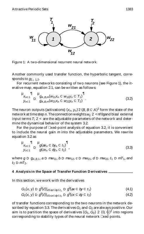
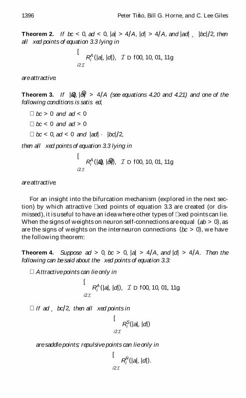
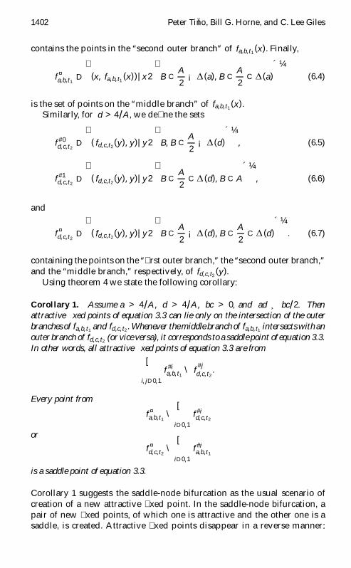


![PERIODIC CLASSIFICATION & PERIODIC PROPERTIES [ 1 ...youvaacademy.com/youvaadmin/image/PERIODIC TABLE BY RS.pdf · [ 2 ] PERIODIC CLASSIFICATION & PERIODIC PROPERTIES BY RAJESH SHAH](https://img.dokumen.tips/doc/110x75/604570870a43592d4f6b3e29/periodic-classification-periodic-properties-1-table-by-rspdf-2.jpg)