Attitude Dynamics and Control of Satellites with

Fluid Ring Actuators

Nona Abolfathi Nobari

Department of Mechanical Engineering

McGill University, Montreal

April, 2013

A thesis submitted to the Faculty of Graduate Studies and Research in partial

fulfillment of the requirements of the degree of Doctor of Philosophy

© Nona Abolfathi Nobari, 2013

Dedicated

to my parents, Shahla and Abbas, for their never-ending incredible

support and sacrifice.

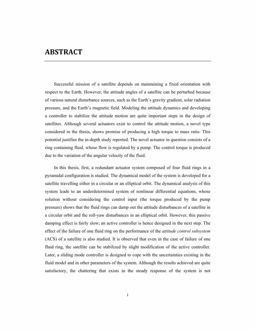
ABSTRACT

Successful mission of a satellite depends on maintaining a fixed orientation with

respect to the Earth. However, the attitude angles of a satellite can be perturbed because

of various natural disturbance sources, such as the Earth’s gravity gradient, solar radiation

pressure, and the Earth’s magnetic field. Modeling the attitude dynamics and developing

a controller to stabilize the attitude motion are quite important steps in the design of

satellites. Although several actuators exist to control the attitude motion, a novel type

considered in the thesis, shows promise of producing a high torque to mass ratio. This

potential justifies the in-depth study reported. The novel actuator in question consists of a

ring containing fluid, whose flow is regulated by a pump. The control torque is produced

due to the variation of the angular velocity of the fluid.

In this thesis, first, a redundant actuator system composed of four fluid rings in a

pyramidal configuration is studied. The dynamical model of the system is developed for a

satellite travelling either in a circular or an elliptical orbit. The dynamical analysis of this

system leads to an underdetermined system of nonlinear differential equations, whose

solution without considering the control input (the torque produced by the pump

pressure) shows that the fluid rings can damp out the attitude disturbances of a satellite in

a circular orbit and the roll-yaw disturbances in an elliptical orbit. However, this passive

damping effect is fairly slow; an active controller is hence designed in the next step. The

effect of the failure of one fluid ring on the performance of the attitude control subsystem

(ACS) of a satellite is also studied. It is observed that even in the case of failure of one

fluid ring, the satellite can be stabilized by slight modification of the active controller.

Later, a sliding mode controller is designed to cope with the uncertainties existing in the

fluid model and in other parameters of the system. Although the results achieved are quite

satisfactory, the chattering that exists in the steady response of the system is not

i

desirable; hence a switching controller consisting of a sliding mode and a PID control law

is designed to eliminate this chattering effect.

Next, the theoretical results obtained are validated by conducting several

experiments. To this end, first, a setup with one fluid ring is designed and built. Here, a

single fluid ring is attached to a disk so as to verify the controllability of the system with

a fluid ring and also the validity of the theoretical model. Although the experimental

results confirm the theory developed in this thesis, the large torque-to-mass ratio expected

is revealed to be only possible at the cost of a quite high input voltage to the pumps

regulating the flow. Therefore, two novel applications of fluid rings are proposed: as an

actuator for spin stabilized satellites, or as an auxiliary actuator in satellites with magnetic

torquers.

Using fluid rings in spin stabilized satellites is proposed in the thesis, as an

alternative to the commonly used micro-thrusters. Here, two fluid rings are mounted on

the satellite while their axes of symmetry are aligned with the roll and yaw axes. To

examine the feasibility and performance, a dynamical model of this spinning satellite

with two fluid rings is developed. A controller is then designed to stabilize the attitude

motion of this satellite.

The second novel actuator system developed here consists in using fluid rings as

complementary actuators in satellites with two magnetic torquers. The dynamical model

is formulated, and a controller is designed to investigate the performance of this system.

The simulation of the system without the fluid ring shows that the satellite attitude can be

stabilized by using only two magnetic torquers, however, slowly. Upon adding the active

fluid ring actuator to the system, the stabilization time is reduced by a factor of 10. The

failure of the fluid ring and each magnetic torquer is also studied.

ii

RÉSUMÉ

La réussite d’une mission d'un satellite dépend du maintien d'une orientation fixe par

rapport à la Terre. Toutefois, les angles d'attitude d'un satellite changent en raison

d’excitations diverses. Un modèle dynamique est utile pour prédire l’attitude du satellite

le développement un contrôleur pour stabiliser l’attitude est également importantes. Un

nouvel actionneur pour le contrôle de l’attitude est proposé dans cette thèse. L’actionneur

fluidique produit un couple élevé par rapport à la masse. L'actionneur en question se

compose d’un anneau rempli par un fluide. L'écoulement de ce fluide est régulé par une

pompe. Le couple de commande est produit par la variation du moment cinétique du

fluide.

Un système d'actionnement redondant composé de quatre anneaux de fluide dans

une configuration pyramidale est d'abord étudié. Le modèle dynamique du système est

développé pour un satellite voyageant dans une orbite circulaire ou elliptique. L'analyse

dynamique de ce système mène à un système sous-déterminé d'équations différentielles

non-linéaires. La solution, sans tenir compte du couple produit par le contrôleur, montre

que les anneaux de fluide peuvent agir comme régulateurs passifs, ce qui amortit les

perturbations d'attitude d’un satellite sur une orbite circulaire et les perturbations en

roulis-lacet selon une orbite elliptique. Cependant, cet effet d'amortissement passif est

assez lent. Par conséquent, le contrôleur actif fut conçu. Les résultats obtenus montrent

que les angles d'attitude du satellite sont stabilisés rapidement. De plus, l'effet de la

défaillance d'un anneau liquide sur la performance du sous-système de contrôle d'attitude

(SCA) du satellite est étudié. On constate que, même dans le cas de défaillance d’un

anneau de fluide, le satellite peut être stabilisé par la modification du contrôleur actif. En

raison des limites de ressources de calcul dans les applications spatiales, un modèle

simple de l'écoulement du fluide est adopté ici. Un contrôleur au mode glissant est donc

conçu pour être robuste aux incertitudes dans le modèle hydraulique et dans les

iii

paramètres du système. Bien que les résultats obtenus soient assez satisfaisants, l’effet

importun du ‘chattering’ existe dans l’état stationnaire du système. Un contrôleur hybride

composé d'un contrôleur au mode glissant avec une loi de commande PID est conçu pour

éliminer cet effet.

Les résultats théoriques sont validés expérimentalement. À cette fin, une première

configuration consistant en un anneau de fluide est conçue et construite. Puis un test sur

un anneau de fluide unique attaché à un disque est effectué pour vérifier si le système

peut être contrôlé, et si le modèle théorique représente le comportement réel. Bien que les

résultats expérimentaux confirment la théorie développée dans cette thèse, le grand

couple à rapport de masse nécessite un coût de tension d'entrée très élevé pour les pompes

de régulation du débit. Par conséquent, deux nouvelles applications d’anneaux de fluide

sont proposées dans cette thèse: comme actionneur pour les satellites stabilisés de spin,

ou comme actionneur auxiliaire avec magnéto-coupleurs.

L’utilisation des anneaux de liquide dans les satellites stabilisés par rotation est le

premier champ d'application proposé comme une alternative aux courants micro-

propulseurs. Dans ce système, deux anneaux de fluide sont montés sur le satellite alors

que leurs axes de symétrie sont alignés avec les directions de roulis et de lacet. Pour

vérifier la faisabilité et la performance, un modèle dynamique de ce satellite en rotation

avec deux anneaux de fluide est développé. Ensuite un contrôleur modifié est conçu pour

stabiliser l’attitude du satellite.

Le deuxième système d’actionneur est développé en utilisant les anneaux de fluide

comme actionneurs complémentaires dans les satellites avec magnéto-coupleurs. Un

modèle dynamique est développé, et un contrôleur est également conçu pour étudier la

performance de ce système. Le système est d’abord examiné sans l'utilisation de l’anneau

de fluide. Les résultats montrent que le satellite est stabilisé par seulement deux magnéto-

coupleurs, mais lentement. Après l’ajout de l'actionneur actif de l’anneau de fluide dans

le système, le temps de stabilisation est réduit par un facteur de dix. L'échec de l’anneau

de fluide et de chaque couple magnétique sont testés.

iv

ACKNOWLEDGEMENTS

First and foremost, I wish to thank my supervisor Professor Arun K. Misra, whose

great knowledge helped me a lot to walk in this path. In fact, this thesis became possible

because of his guidance and support. By now, not only he is my professional role-model

for his knowledge, but also for his kind treatment. Indeed, his patience and kindness

softened the difficult days of PhD studies. With his fatherly behaviour, he taught me how

to enter and remain in the research world.

I could never imagine that someone can make me feel like I have a brother, until I

met Dr. Bijan Deris. His encouragement and support made the life in Montreal much

more pleasant. The fact that, at every moment of a day or a night, he has always been

open to receive me and my husband is very sweet. I also wish to thank his wife, Shiva

Varshovi, for her peaceful personality that calmed me down and sweetened the

unpleasant taste of the difficult moments of my graduate student life.

I wish to thank Sara Shayan Amin, who has always been there for me when I needed

her the most. She, with her high energy, was a boost for me to walk in this path more and

more strongly. For the first time in Montreal, she gave me the sweet taste of having a

close friend. She is one of the reasons that living in Montreal became more pleasant for

me. I would also like to thank Dr. Hamid Dalir, whose optimism always motivated me

toward my goals.

I thank Dr. Afshin Taghvaiepour: as a very good friend, he helped me to be much

more aware of different aspects of human personality, and thus, to try to improve mine. In

the first days in Montreal, I and my husband were received by a close friend, Tara Khani,

v

and his husband, Majid Fekri. Their kindness cannot be forgotten as they helped me to

start my PhD without worrying about a shelter in the very first days.

I want to thank Tara Mirmohammadi, Pamela Woo, and Mohammad Jalali

Mashayekhi because of their helps and also the friendly environment they made at the

office. I also would like to thank Bahareh Ghotbi, Atefeh Nabavi, and Nazanin Aghaloo

because of all pleasing moments that we had together all this time. I would also like to

thank Mehdi Paak and Dr. Vahid Raeesi for our technical discussions on fluid structure

interactions and robust controller design.

I wish to thank my father- and mother-in-law, Mr. Ebrahim Alizadeh and Taraneh

Yarahmadi, for their everyday support. I am always aware of their kindness in treating me

like a princess and wishing me all the best of the worlds. Not only because of that, but

also I want to thank them mostly because of their son, Danial, whose unconditional

support has always been there for me. During all this time, Danial got so tough on

himself to soften the way ahead of me as much as he could. My sister, Nila, with her

everyday phone calls and kind voice unbelievably reduced the sadness of being far apart.

She always stayed beside me in my happiness, sadness and became a great support from

thousands of miles away. Finally, I reached to my parents, Shahla and Abbas; I thank

them at the end, because I believe in their patience. I owed my success to my parents

because of their incredible support and sacrifice. One should be a parent to understand the

meaning of the unconditional love that they always offered me. In fact, only hearing “my

daughter” from them was more than enough to forget all the sorrow. Mom and dad: I

love you because of everything you did, which I cannot describe; I dedicate this thesis to

you.

vi

CLAIM OF ORIGINALITY

The originality of the main ideas and research results presented in this thesis are

claimed here. The most significant ones are listed below:

(i) The main claim of novelty of this thesis is that, for the first time, a

thorough feasibility analysis of using fluid ring systems for attitude

control is reported, which highlights the advantages of this system

quantitatively.

(ii) A more accurate dynamical model compared to what exists in the

literature is developed for a system consisting of a satellite and a set of

fluid ring actuators.

(iii) Although a PID controller could stabilize the system understudy, another

contribution of the thesis is to propose a switching application of a

sliding mode controller and a PID so as to cope with the model

uncertainties and avoid chattering in the system response.

(iv) The feasibility of using fluid ring actuators was demonstrated through the

experiments.

(v) A novel application of fluid ring actuators is suggested that indicates

using fluid rings for stabilizing the attitude angles of spinning satellites.

Henceforth, a dynamical model is developed and a controller is designed

for the system proposed.

(vi) A new hybrid actuator consisting of a fluid ring and two magnetic

torquers is proposed. Moreover, the dynamical model of this system is

developed; the effect of failure of an actuator of this new hybrid system

was also evaluated.

vii

viii

NOMENCLATURE

Roman symbols

A Fluid ring cross-sectional area

𝒃 Earth’s geomagnetic field vector

𝑐1 , 𝑐2 Non–dimensional physical parameters defined in Eqs. (2.24) and (5.35)

𝑑 Cross-sectional diameter of fluid rings

�̂� Non–dimensional geometric parameter of fluid rings defined in Eqs. (2.24) and (5.35)

𝑒 Orbit eccentricity

𝑓 Friction coefficient

𝐼𝑎, 𝐼𝑡 Moments of inertia of a spinning satellite in axial and tangential directions

𝐼𝑑 Moment of inertia of a disk

𝐼𝑓 Fluid moment of inertia

𝑰𝒇𝒊 Inertia matrix of the 𝑖 th fluid ring about its axis of symmetry

𝑰�𝒇𝒊 Non-dimensional inertia matrix of the 𝑖th fluid ring

ix

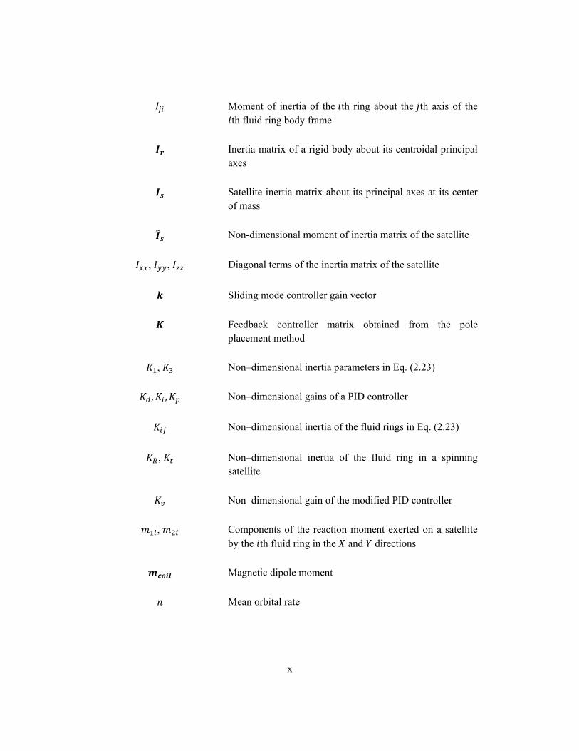
𝐼𝑗𝑖 Moment of inertia of the 𝑖th ring about the 𝑗th axis of the 𝑖th fluid ring body frame

𝑰𝒓 Inertia matrix of a rigid body about its centroidal principal axes

𝑰𝒔 Satellite inertia matrix about its principal axes at its center of mass

𝑰�𝒔 Non-dimensional moment of inertia matrix of the satellite

𝐼𝑥𝑥, 𝐼𝑦𝑦, 𝐼𝑧𝑧 Diagonal terms of the inertia matrix of the satellite

𝒌 Sliding mode controller gain vector

𝑲 Feedback controller matrix obtained from the pole placement method

𝐾1, 𝐾3 Non–dimensional inertia parameters in Eq. (2.23)

𝐾𝑑 ,𝐾𝑖 ,𝐾𝑝 Non–dimensional gains of a PID controller

𝐾𝑖𝑗 Non–dimensional inertia of the fluid rings in Eq. (2.23)

𝐾𝑅, 𝐾𝑡 Non–dimensional inertia of the fluid ring in a spinning satellite

𝐾𝑣 Non–dimensional gain of the modified PID controller

𝑚1𝑖, 𝑚2𝑖 Components of the reaction moment exerted on a satellite by the 𝑖th fluid ring in the 𝑋 and 𝑌 directions

𝒎𝒄𝒐𝒊𝒍 Magnetic dipole moment

𝑛 Mean orbital rate

x

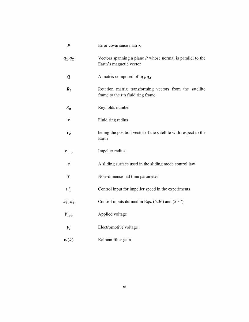
𝑷 Error covariance matrix

𝒒𝟏,𝒒𝟐 Vectors spanning a plane 𝑃 whose normal is parallel to the Earth’s magnetic vector

𝑸 A matrix composed of 𝒒𝟏,𝒒𝟐

𝑹𝒊 Rotation matrix transforming vectors from the satellite frame to the 𝑖th fluid ring frame

𝑅𝑛 Reynolds number

𝑟 Fluid ring radius

𝒓𝒄 beimg the position vector of the satellite with respect to the Earth

𝑟𝑖𝑚𝑝 Impeller radius

𝑠 A sliding surface used in the sliding mode control law

𝑇 Non–dimensional time parameter

𝑢𝜔𝑐 Control input for impeller speed in the experiments

𝑣1𝑐, 𝑣3𝑐 Control inputs defined in Eqs. (5.36) and (5.37)

𝑉𝑎𝑝𝑝 Applied voltage

𝑉𝑒 Electromotive voltage

𝒘(𝑘) Kalman filter gain

xi

Greek symbols

𝛼𝑖, 𝛾𝑖 Pyramidal configuration angles (Euler angles describing the orientation of the 𝑖th fluid ring)

�̇� Fluid angular velocity

�̇�𝑖 Fluid angular velocity relative to the 𝑖th ring

𝛽𝑖′ Non-dimensional fluid angular velocity

𝛿 Error signal

𝜂𝑖 Sliding mode gain

𝜃 Disk angle

𝜃𝑖 Attitude angles of the satellite, 𝑖 = 𝑥, 𝑦, 𝑧

𝜽 Array of attitude angles of the satellite

𝜽′ Non-dimensional rate of attitude angles array

𝜽𝒅 Array of desired attitude angles

Θ, Θ̇ True anomaly and orbital rate

Θ′ Non-dimensional orbital rate

𝜆 Design parameter of the sliding mode controller

𝜇 Fluid viscosity

𝜈 Ω + 𝑛

𝜉 Damping factor

xii

𝜌 Fluid density

𝜎 Fluid shear stress acting on the wall of the ring

𝜏𝑐 Control torque

�̂�𝑐 Non-dimensional control torque

𝜏𝑎 Torque produced by a fluid ring

𝝉𝒆𝒙𝒕 External torque exerted on a satellite

𝜏𝑓 Fluid friction torque

𝜏𝑓𝑖 Fluid friction torque in the 𝑖th ring

�̂�𝑓𝑖 Non-dimensional fluid friction torque in the 𝑖th ring

𝝉𝒈𝒕 Gravity gradient torque exerted on the satellite

𝝉�𝒈𝒕 Non-dimensional gravity gradient torque exerted on the satellite

𝝉𝒈𝒕𝒇𝒊 Gravity gradient torque exerted on the fluid rings

𝝉�𝒈𝒕𝒇𝒊 Non-dimensional gravity gradient torque exerted on the fluid rings

𝝉𝒎 Magnetic torque

𝜏𝑝

𝝉𝒓

Pump pressure torque

Reaction torque

𝝎 Satellite angular velocity defined in its own body frame

xiii

𝝎� Non-dimensional angular velocity of the satellite

𝝎𝒇 The absolute angular velocity of the fluid defined in the body frame of the fluid ring

𝜔𝑖𝑚𝑝 Impeller angular velocity

Ω Spin rate of a spinning satellite

xiv

TABLE OF CONTENTS

ABSTRACT ......................................................................................................................... i

RÉSUMÉ ........................................................................................................................... iii

ACKNOWLEDGEMENTS ................................................................................................ v

CLAIM OF ORIGINALITY ............................................................................................. vii

NOMENCLATURE .......................................................................................................... ix

TABLE OF CONTENTS .................................................................................................. xv

TABLE OF FIGURES ..................................................................................................... xix

TABLE OF TABLES ................................................................................................... xxvii

INTRODUCTION .............................................................................................................. 1

1.1 Background ............................................................................................................ 1

1.1.1. Reaction/Momentum Wheels ........................................................................ 2

1.1.2. Control Moment Gyros ................................................................................. 4

1.1.3. Micro-thrusters .............................................................................................. 5

1.1.4. Magnetic Torque Rod Actuators ................................................................... 6

1.2. Motivation .............................................................................................................. 7

1.3. Review of the Literature on Fluidic Actuators ....................................................... 8

1.4. Objectives of the Thesis ....................................................................................... 11

1.5. Thesis Organization ............................................................................................. 11

ATTITUDE DYNAMICS OF A RIGID SATELLITE WITH FLUID RINGS ............... 13

2.2 Dynamical Model of a Rigid Satellite with Fluid Rings ...................................... 13

xv

2.1.1. Non-dimensionalization of the equations of motion ................................... 19

2.3 Numerical Results with Passive Fluid Rings ....................................................... 21

2.4 Summary .............................................................................................................. 29

DESIGNING OF CONTROLLERS FOR SATELLITES WITH FLUID RINGS ........... 31

3.1 PID Controller ...................................................................................................... 32

3.2. Failure Analysis ................................................................................................... 38

3.3. Designing a Sliding Mode Controller .................................................................. 41

3.3.1. Dynamical behaviour of the system with the sliding mode controller ........ 44

3.4. Switching Control Law ........................................................................................ 46

3.5. Summary .............................................................................................................. 48

EXPERIMENTAL RESULTS .......................................................................................... 49

4.1. Design of the Experimental Setup ....................................................................... 49

4.1.1. Material selection ........................................................................................ 50

4.1.2. Fluid selection ............................................................................................. 50

4.1.3. Pump selection ............................................................................................ 51

4.2. Preliminary Analysis ............................................................................................ 52

4.3. Experiment with a Single Fluid Ring System ...................................................... 55

4.3.1. Designing a Kalman filter ........................................................................... 56

4.3.2. Single fluid ring system experiment ............................................................ 59

4.4. Three Dimensional (3D) Control Experiment ..................................................... 63

4.5. Summary .............................................................................................................. 68

SPINNING SATELLITES WITH FLUID RING ACTUATORS .................................... 69

5.1. Development of the Dynamical Model ................................................................ 70

5.2. Small Angle Approximation ................................................................................ 73

xvi

5.2.1. Non-dimensionalization .............................................................................. 76

5.3. Design of a Controller for the Linear Model ....................................................... 77

5.3.1. Numerical results for the linear model ........................................................ 79

5.4. Design of the Controller for the Nonlinear Model ............................................... 81

5.4.1. Numerical results for the nonlinear system ................................................. 82

5.5. Summary .............................................................................................................. 85

A HYBRID ATTITUDE CONTROLLER CONSISTING OF ECTROMAGNETIC TORQUE RODS AND A FLUID RING ............................................................... 87

6.1. Dynamics Modeling ............................................................................................. 88

6.2. Simulation and Results ........................................................................................ 93

6.3. Failure Study ........................................................................................................ 97

6.3.1. Failure of the fluid ring ............................................................................... 98

6.3.2. Failure of one magnetic coil ...................................................................... 101

6.4. Summary ............................................................................................................ 105

CONCLUDING REMARKS AND RECOMMENDATIONS FOR FUTURE WORK 107

7.1. Summary and Findings ...................................................................................... 108

7.2. Recommendations for Future Work ................................................................... 110

REFERENCES ............................................................................................................... 111

xvii

xviii

TABLE OF FIGURES

Figure 1.1: A reaction/momentum wheel (Wertz, 1999) .................................................... 3

Figure 1.2: Singular configuration of CMGs (Leeghim et al. 2009) ................................... 5

Figure 1.3: Magnetic torquer designed by Vectronic Aerospace ........................................ 6

Figure 1.4: A fluid ring actuator (Patel and Kumar, 2009) ................................................ 8

Figure 1.5: Fluidic actuator proposed by Maynard (1988) ................................................. 9

Figure 1.6: Fluid loop configurations proposed by Lurie et al. (1991) ............................... 9

Figure 1.7: A dual-function actuator consisting of a fluid loop and a permanent magnet 10

Figure 1.8: Fluid loop prototype used by Kelly et al. (2004) ............................................ 10

Figure 2.1: A satellite with three orthogonal fluid rings ................................................... 14

Figure 2.2: Pyramidal configuration of the fluid rings in a satellite ................................. 15

Figure 2.3: (a) LVLH reference frame of a satellite; (b) Free body diagram of a fluid ring ................................................................................................................................ 15

Figure 2.4: Attitude motion of the satellite in a circular orbit in the absence of damping torques: (a) Roll angle; (b) Pitch angle; (c) Yaw angle .................................................... 22

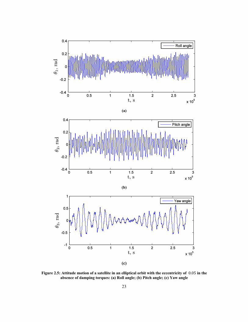
Figure 2.5: Attitude motion of a satellite in an elliptical orbit with the eccentricity of 0.05 in the absence of damping torques: (a) Roll angle; (b) Pitch angle; (c) Yaw angle . 23

Figure 2.6: Attitude motion of the satellite in a circular orbit in the presence of damping torques of four fluid rings: (a) Roll angle; (b) Pitch angle; (c) Yaw angle ............. 24

Figure 2.7: Attitude motion of a satellite in an elliptical orbit with the eccentricity of 0.05 in the presence of damping torques of four fluid rings: (a) Roll angle; (b) Pitch angle; (c) Yaw angle ...................................................................................... 25

Figure 2.8: Attitude angles for the pyramidal angle 𝛾 = 5°: (a) Roll angle; (b) Pitch angle; (c) Yaw angle .......................................................................................................... 26

xix

Figure 2.9: Attitude angles for the pyramidal angle 𝛾 = 45°: (a) Roll angle; (b) Pitch angle; (c) Yaw angle ............................................................................................... 27

Figure 2.10: Attitude angles for the pyramidal angle𝛾=𝟖𝟓°: (a) Roll angle; (b) Pitch

angle; (c) Yaw angle ............................................................................................... 27

Figure 3.1: Attitude angles of the controlled system with PID gains 𝐾𝑝 = 5000, 𝐾𝑑 = 10, and 𝐾𝑖 = 0.5 (circular orbit): (a) Roll angle; (b) Pitch angle; (c) Yaw angle ......... 33

Figure 3.2: Control torque components with PID gains 𝐾𝑝 = 5000, 𝐾𝑑 = 10, and 𝐾𝑖 = 0.5 (circular orbit case); (a) Roll angle; (b) Pitch angle; (c) Yaw angle ........ 34

Figure 3.3: Fluid angular velocity with PID gains 𝐾𝑝 = 5000 , 𝐾𝑑 = 10, and 𝐾𝑖 = 0.5 (circular orbit case) ................................................................................................. 35

Figure 3.4: Attitude angles of the controlled system with various pyramidal angles using ................................................................................................................................ 36

Figure 3.5: Attitude angle differences upon varying the pyramidal angle 𝛾 with PID gains Kp = 5000, Kd = 10, and 𝐾𝑖 = 0.5 : (a) Difference of attitude angles between 𝛾 = 5° and 45°; (b) Difference of attitude angles between 𝛾 = 45° and 85° (circular orbit case) .......................................................................................... 37

Figure 3.6: Response of the system subject to the failure of one fluid ring with using PID gains 𝐾𝑝 = 5000 , 𝐾𝑑 = 10, and 𝐾𝑖 = 0.5 (circular orbit case): (a) Satellite attitude angles; (b) Fluid angular velocity in the rings; (c) Resultant control torque ................................................................................................................................ 39

Figure 3.7: Response of the system associated with the failure of one fluid ring using the gains 𝐾𝑝 = 5000 , 𝐾𝑑 = 10, 𝐾𝑖 = 0.5, and 𝐾𝑣 = −0.5 (circular orbit case): (a) Satellite attitude angles; (b) Fluid angular velocity in the rings; (c) Control torque ................................................................................................................................ 40

Figure 3.8: Sliding hypersurface for the roll direction ...................................................... 42

Figure 3.9: Attitude angles after applying the sliding mode controller (circular orbit case) ................................................................................................................................ 44

Figure 3.10: Components of the control torque resulting from the sliding mode controller: (a) Roll direction; (b) Pitch direction; (c) Yaw direction (circular orbit case) ....... 45

Figure 3.11: Attitude angles after applying the switching controller (circular orbit case) 46

xx

Figure 3.12: Control torque resulting from the switching controller; (a) Roll direction; (b) Pitch direction; (c) Yaw direction (circular orbit case) .......................................... 47

Figure 3.13: Satellite attitude angles using a PID controller with the nominal parameter values ...................................................................................................................... 48

Figure 3.14: Satellite attitude angles using a PID controller subject to the ±15% uncertainty in the nominal parameter values .......................................................... 48

Figure 4.1: The fluid ring used in the experimental validation phase ............................... 52

Figure 4.2: Angular velocity of the impeller versus the applied voltage .......................... 53

Figure 4.3: Fluid ring with its base mounted on the simulator ......................................... 54

Figure 4.4: Fluid angular velocity �̇� versus the impeller angular velocity 𝜔𝑖𝑚𝑝 using a sinusoidal input voltage .......................................................................................... 54

Figure 4.5: The block diagram of the controllers used between the model and the plant . 56

Figure 4.6: The block diagram of a system with a Kalman filter ...................................... 56

Figure 4.7: Theoretical and experimental plots of the impeller angular velocity versus time ......................................................................................................................... 61

Figure 4.8: Theoretical and experimental plots of the attitude angle of the disk versus time ......................................................................................................................... 61

Figure 4.9: The theoretical and experimental plots of the disk angular velocity versus time ................................................................................................................................ 62

Figure 4.10: The experimental control torque versus time ............................................... 62

Figure 4.11: Input voltage which is applied to the fluid ring system ................................ 62

Figure 4.12: (a) Cubic satellite floating on the simulator; (b) Hardware-in-the-loop experimental setup .................................................................................................. 63

Figure 4.13: Attitude angles found from the theoretical model ........................................ 64

Figure 4.14: Theoretical and Experimental angular velocities of the roll-axis impeller ... 64

Figure 4.15: Theoretical and Experimental angular velocities of the pitch-axis impeller 64

Figure 4.16: Theoretical and Experimental angular velocities of the yaw-axis impeller .. 65

xxi

Figure 4.17: Desired fluid angular velocity in the: (a) Roll-axis ring; (b) Pitch-axis ring; (c) Yaw-axis ring .................................................................................................... 66

Figure 4.18: Applied voltage to the pumps on different rings versus time: (a) roll-axis; (b) pitch-axis; (c) yaw axis ........................................................................................... 67

Figure 5.1: A cylindrical satellite with two fluid rings ..................................................... 70

Figure 5.2: Three coordinates frames used in dynamical modeling ................................. 71

Figure 5.3: Free body diagrams of the satellite and two fluid rings (only moment vectors are shown) ............................................................................................................... 71

Figure 5.4: Roll and yaw angles using the linear controller with 𝑝𝑖 = −10 ..................... 80

Figure 5.5: Control torque in the roll and yaw directions using the linear controller with 𝑝𝑖 = −10 ................................................................................................................. 80

Figure 5.6: Fluid angular velocity using the linear controller with 𝑝𝑖 = −10 .................. 80

Figure 5.7: Pitch angle 𝜃2 while using the modified PD controller with the gains obtained from the linear controller: 𝐾𝑝1𝑖 = 364; 𝐾𝑑1𝑖 = −25; 𝐾𝑝2𝑖 =140; and 𝐾𝑑2𝑖 = −23 ................................................................................................................................ 83

Figure 5.8: Roll and yaw angles (𝜃1 and 𝜃3), while utilizing the modified PD controller with the gains obtained from the linear controller: 𝐾𝑝1𝑖 = 364 ; 𝐾𝑑1𝑖 =−25; 𝐾𝑝2𝑖 =140; and 𝐾𝑑2𝑖 = −23 .......................................................................... 83

Figure 5.9: Control torque produced by the modified PD controller with the gains obtained from the linear controller: 𝐾𝑝1𝑖 = 364 ; 𝐾𝑑1𝑖 = − 25; 𝐾𝑝2𝑖 = 140; and 𝐾𝑑2𝑖 = −23 ...................................................................................................... 83

Figure 5.10: Angular velocity of the fluid, while using the modified PD controller with the gains obtained in the linear controller: 𝐾𝑝1𝑖 = 364; 𝐾𝑑1𝑖 = −25; 𝐾𝑝2𝑖 =140; and 𝐾𝑑2𝑖 = −23 ...................................................................................................... 84

Figure 5.11: Roll and yaw angles (𝜃1 and 𝜃3), while using the modified PD controller with the gains of 𝐾𝑝1𝑖 = 350 ; 𝐾𝑝2𝑖 = 140 ; 𝐾𝑑11 = −25; 𝐾𝑑21 =−5; 𝐾𝑑12=−5; and 𝐾𝑑22 = −25 ............................................ 84

Figure 5.12: Control torque produced by the modified PD controller with the gains of 𝐾𝑝1𝑖 = 350; 𝐾𝑝2𝑖 = 140; 𝐾𝑑11 = −25; 𝐾𝑑21 =−5; 𝐾𝑑12=−5; and 𝐾𝑑22 = −25 . 85

xxii

Figure 5.13: : Angular velocity of the fluid, while using the modified PD controller with the gains of 𝐾𝑝1𝑖 = 350 ; 𝐾𝑝2𝑖 = 140 ; 𝐾𝑑11 = −25; 𝐾𝑑21 =−5; 𝐾𝑑12=−5; and 𝐾𝑑22 = −25 ............................................ 85

Figure 6.1: A satellite with two magnetic coils and one fluid ring ................................... 88

Figure 6.2: The control torque vector decomposition ....................................................... 89

Figure 6.3: The attitude angles of a satellite using two magnetic coils with PID gains 𝐾𝑝 = 50, 𝐾𝑑 = 60, and 𝐾𝑖 = 1 .................................................................... 93

Figure 6.4: Torques produced in the satellite using only two magnetic coils with PID gains 𝐾𝑝 = 50, 𝐾𝑑 = 60, and 𝐾𝑖 = 1: (a) Control torque; (b) Torque produced by the magnetic coils in the roll direction; (c) Torque produced by the magnetic coils in the pitch direction; (d) Torque produced by the magnetic coils in the yaw direction; (e) Magnetic dipole moments ................................................................. 94

Figure 6.5: The attitude angles of a satellite using two magnetic coils and one active fluid ring with PID gains 𝐾𝑝 = 70, 𝐾𝑑 = 100, and 𝐾𝑖 = 0 ........................................... 95

Figure 6.6: Torques produced in the satellite using two magnetic coils and one fluid ring with PID gains 𝐾𝑝 = 70, 𝐾𝑑 = 100, and 𝐾𝑖 = 0: (a) Control torque; (b) Torque produced by the pump; (c) Fluid friction torque; (d) Torque produced by the magnetic coils; (e) Magnetic dipole moments ........................................................ 97

Figure 6.7: Attitude angles of the satellite in the case of failure of the fluid ring with PID gains 𝐾𝑝 = 60, 𝐾𝑑 = 30, and 𝐾𝑖 = 1 .................................................................... 98

Figure 6.8: Torque produced in the satellite with the fluid ring failure with PID gains 𝐾𝑝 = 60, 𝐾𝑑 = 30, and 𝐾𝑖 = 1: (a) Control torque; (b) Fluid friction torque; (c) Torque produced by the magnetic coils;(d) Magnetic dipole moments .......... 100

Figure 6.9: Stabilization of attitude angles in the case of failure of the roll-axis magnetic coil with PID gains 𝐾𝑝 = 12, 𝐾𝑑 = 2, and 𝐾𝑖 = 0.01 .......................................... 101

Figure 6.10: The torque produced in the case of failure of the roll-axis coil with PID gains 𝐾𝑝 = 12, 𝐾𝑑 = 2, and 𝐾𝑖 = 0.01: (a) Control torque; (b) Torque produced by the fluid ring; (c) Torque produced by the magnetic coils; (d) Magnetic dipole moment in the pitch direction ............................................................................... 102

Figure 6.11: Stabilization of attitude angles in the case of failure of the pitch-axis coil with PID gains 𝐾𝑝 = 450, 𝐾𝑑 = 15, and 𝐾𝑖 = 0.01 ........................................... 103

xxiii

Figure 6.12: Torques produced in the case of failure of the pitch-axis coil with PID gains 𝐾𝑝 = 450, 𝐾𝑑 = 15, and 𝐾𝑖 = 0.01: (a) Control torque; (b) Torque produced by the fluid ring; (c) Magnetic dipole moment in the roll direction; (d) Torque produced by the magnetic coils ............................................................................ 104

xxiv

TABLE OF TABLES

Table 2.1: Stability condition of a satellite in a circular orbit ........................................................ 28

Table 2.2: Stability condition of a satellite in an elliptical orbit with the eccentricity of 0.05 ..... 28

Table 4.1: Fluid properties ............................................................................................................. 50

Chapter 1

INTRODUCTION

1.1 Background

A satellite is required to maintain a specific orientation in order to complete its mission

objectives, such as communication and imaging. However, the satellite attitude can be disturbed

due to different natural sources, such as the Earth’s gravity gradient, solar radiation pressure,

aerodynamic forces, and the Earth’s magnetic field. These disturbances usually cause rotational

oscillations of the satellite, but at times they can cause the satellite to tumble. To avoid this, the

design of any satellite should include an attitude stabilization scheme, which normally involves

an attitude control subsystem.

Several methods of attitude stabilization of satellites have been developed over the last five

decades, which can be divided into two groups: passive and active. The most fundamental passive

method is gravity gradient stabilization (Wie, 1998). In this method, the principal axes of the

satellite are required to be aligned with the local vertical and local horizontal (LVLH) reference

frame whose origin is located at the center of mass of the satellite. The axes of maximum and

1

minimum moment of inertia should be aligned with the axes which are perpendicular to the

orbital plane and directed to the center of the Earth. If this condition holds, the satellite attitude

angles remain stable even in the presence of small perturbations (Wie, 1998).

Another passive stabilization method is to spin up a satellite about one of its principal axes.

In fact, spinning causes the satellite to resist changing its attitude (Hughes, 1986). The reason

behind is that the disturbance torques are not large enough to significantly change the direction of

the bias angular momentum produced in the spinning direction.

Other passive methods involve energy dissipation, such as using liquid, magnetic, or

nutation dampers to reduce the attitude variations. However, it should be pointed out that energy

dissipation can sometimes be destabilizing. For instance, a satellite spinning about its axis of

minimum moment of inertia can become unstable, if energy dissipation occurs (Leimanis, 1965;

Hughes, 1986; and Fortescue and Stark, 1995).

There are some drawbacks in relying on passive methods as the primary techniques of

attitude stabilization, such as their slow action and their lack of ability for tracking desired

attitude. Therefore, passive methods are often utilized only to improve the performance of active

methods. In fact, the focus of research on satellite attitude dynamics and control is generally on

the active alternatives; hence, a literature survey on these methods is in order.

1.1.1. Reaction/Momentum Wheels

Reaction wheels, momentum wheels, or control moment gyros are the most common attitude

actuators utilized in satellites. A reaction wheel has zero initial angular velocity; a resistant torque

can be produced by accelerating or decelerating the rotation of the wheel. Momentum wheels are

the counterpart of reaction wheels; they have a non-zero initial angular velocity, by changing

which the magnitude of the resistance torque can be controlled1 (Schaub and Junkins, 2003).

Figure 1.1 shows a reaction/momentum wheel.

There are some drawbacks associated with reaction and momentum wheels, such as their

relatively small capacity to produce torque and also the saturation problem (Wie, 1998). The

1 Although control moment gyros are modifications of simple momentum wheels, they are considered here as another type of attitude control actuators and will be discussed later.

2

latter implies that the wheel cannot speed up any further so as to produce larger torques; in fact,

the saturation occurs because of various restrictions, such as motor maximum capability, bearing

friction, and maximum voltage available. Despite the abovementioned disadvantages, due to their

simple functionality and control, these actuators are commonly used in the space industry.

Extensive research has been conducted on reaction/momentum wheels so as to minimize their

energy consumption and improve their performance (Kaplan, 1976; Barba and Aurbrun, 1976;

Hablani, 1994; Tsiotras et al. 2001; Richie and Lappas, 2007; Zhang et al. 2009; Navabi and

Nasiri, 2010; Ye et al. 2011).

Figure 1.1: A reaction/momentum wheel (Wertz, 1999)

Optimization of the configuration of a set of reaction/momentum wheels used in a satellite is

also a subject of interest. Recently, Ismail and Varatharajoo (2010) examined different

configurations of reaction wheels in a satellite in order to find the optimum configuration based

on the power consumption and the momentum produced. They proposed 11 different structures

with three reaction wheels, for which the dynamical models were developed and PD controllers

were designed. The same procedure was followed for four reaction wheels in eight different

configurations. The results showed that there is no significant difference in the momentum

produced in various cases, the minimum total torque level also varying only slightly. It was

shown that the pyramidal configuration of four reaction wheels is neither an optimum nor the

worst case. However, the pyramidal configuration is used in several research articles (Marshall et

al. 1991; Hablani, 1994; Lee et al. 2009; Li and Kumar 2011), the reason for this selection being

the symmetry of the system that proves helpful in the case of failure of a control actuator.

Due to its high importance, the failure analysis of control actuators is thoroughly discussed

in the literature (Vadali and Junkins, 1984; Hablani, 1994; Battagliere et al. 2010; Haga and Saleh

3

2011; Horri and Palmer, 2012). For instance, Godard et al. (2010) studied this problem by

considering a redundant set of four reaction wheels in a satellite. In their model, they also

considered saturation of the reaction wheels, external disturbance torques, and model

uncertainties. To control the satellite in the case of failure of one reaction wheel, they designed an

adaptive controller. The results were validated with a hardware-in-the-loop simulation, which

proved the robustness of the control algorithm proposed.

1.1.2. Control Moment Gyros

Control moment gyros (CMGs) are the momentum wheels with the capability of rotating

about two axes: the axis of symmetry and an axis orthogonal to the former. In this type of

actuators, the spinning rate of the wheel is fixed, the effective torque being produced via rotating

the wheel about the second axis, called the gimbal axis (Schaub and Junkins, 2003). This

operation allows producing quite large torques, which makes CMGs the most desirable choice in

agile space systems. The most significant disadvantage of CMGs is that they have singularities at

certain gimbal angles which are perpendicular to the plane of the allowable torques (Figure 1.2).

At the singularities, CMGs cannot produce the torque required, despite consuming more energy.

Different control strategies have been proposed to avoid these singularities or, at least, handle

them efficiently (Kennel, 1970; Li and Bainum, 1990; Krishnan and Vadali, 1996; Kurokawa,

1997; McMahon and Schaub 2010; Leeghim and Park 2009; Lappas and Wie 2009; Akiyama

2010). For example, Sands et al. (2009) developed a decoupled control strategy to solve the

singularity problem of CMGs. The theoretical results were verified by an experiment in which the

simulator test bed allows for a free-floating satellite. As an alternative solution, Nanamori et al.

(2008) suggested using a geometric method to solve the singularity problem. In this method, the

initial gimbal angles were chosen by an optimization algorithm, so as to reduce the possibility of

falling into singularities in the operation range of the CMGs.

4

Figure 1.2: Singular configuration of CMGs (Leeghim et al. 2009)

A few researchers have suggested using double-gimbal CMGs to avoid singularities (Wie,

1998; Ahmed and Bernstein, 2002; Bolandi et al., 2006), a solution that is more costly and

complex for the dynamical modeling view point(Wie, 1998). McMahon and Schaub (2010),

Richie and Lappas (2007), and Jin and Hwang (2011) have designed variable-speed control

moment gyroscopes to produce the exact effective torque required at the cost of increasing the

difficulty of dynamical modelling and controller design.

1.1.3. Micro-thrusters

Micro-thrusters are another type of attitude actuators, which are of considerable importance

for their low modeling complexity. For more than four decades, these actuators have been utilized

in various types of satellites (Kazinczy and Leibing, 1975; Stenmark and Lang, 1997), such as

spinning satellites ( Jiang et al. 2008; Raus et al. 2010; Ayoubi and Longuski 2009). For instance,

recently, Tang et al. (2011) used micro-thruster actuators in a small spinning satellite for the

three-dimensional attitude control. The authors suggested a dual-phase fuel thruster, which is

composed of compressed cold-gas and liquid nitrogen. Srikant and Akella (2010) used cold-gas

proportional thrusters for the control of attitude motion of a satellite. Micro-thrusters can also be

augmented by other types of attitude actuators; as an example, Liu et al. (2010) suggested a

combination of thrusters and a single-pitch bias momentum wheel for attitude control.

5

1.1.4. Magnetic Torque Rod Actuators

The Earth’s magnetic field was introduced earlier in this chapter as a source of

environmental disturbance. On the other hand, this effect has been used for satellite attitude

stabilization for more than four decades (Steyn, 1994; Maeda et al., 1997; Sun et al., 2003; Hur-

Diaz et al. 2008; Forbes and Damaren 2010; Kataoka and Kawai 2010; Kim et al. 2011). A

magnetic torque rod, also known as magnetic torquer, is an actuator (Figure 1.3), which produces

torque by interacting with the Earth’s magnetic field.

Figure 1.3: Magnetic torquer designed by Vectronic Aerospace

Indeed, a magnetic torquer is a rod core wrapped by an electric conductor. In the presence of

a magnetic field and electric current in the wire, a torque is produced. The simple functionality,

low mass, and low energy consumption have made magnetic torquers quite popular for

applications in small satellites (Steyn, 1994; Maeda et al., 1997; Sun et al., 2003).

The drawback of magnetic torquers is that they cannot produce torque in the direction of the

geomagnetic field vector. Moreover, the estimation of the magnitude of the geomagnetic field

vector is not accurate, something which reduces the accuracy of attitude stabilization. In the

literature, the means of increasing the accuracy of magnetic torque rods and also producing

torque in all directions have been investigated (Hur-Diaz et al. 2008; Forbes and Damaren 2010;

De Ruiter 2011). For instance, De Ruiter (2011) studied a spinning satellite equipped with three

magnetic torque rods mounted on three directions of roll, pitch, and yaw. The failure of one or

two magnetic torquers was then handled by modifying the control law developed for the complete

system. Das et al. (2010) studied the performance of three magnetic torquers in a small satellite.

They also considered the case of failure of one magnetic torquer, for which a modified control

law was designed. Wang et al. (2010) combined a passive stabilizer method, based on

aerodynamics drag, with magnetic torquers to control the satellite attitude angles. To exploit the

6

drag force in attitude stabilization, these researchers determined the appropriate position of the

center of pressure and the centroid of a satellite. The results showed that this hybrid controller can

asymptotically stabilize the attitude motion.

Chen et al. (2008), and Soyali and Jafarov (2011) compared the performance of two different

actuator systems: a system including only magnetic torquers; another combining magnetic

torquers with a bias momentum wheel. The results showed that the settling time and power

consumption is lower, for the former case, while adding a bias momentum wheel can reduce the

steady-state error. Further, Forbes and Damaren (2010) considered a combination of magnetic

torquers and reaction wheels as control actuators for attitude stabilization. They calculated the

torque to be produced by different components via decomposing the control torque: the

component of the control torque parallel to the Earth’s magnetic field vector is produced by

reaction wheels, the rest by the magnetic torquers. They studied the cases of using one, two, and

three reaction wheels. The results are significant, especially in the case of saturation of the

reaction wheels.

1.2. Motivation

As mentioned in Section 1.1, several methods of attitude stabilization, passive or active,

have been developed so far. Among various active methods, wheels, being currently the most

popular type, are typically used either as reaction/momentum wheels or CMGs. The downside of

reaction wheels is that they do not produce a large torque to mass ratio. The CMGs are much

better in this regard, their main drawback being the existence of singularities at some gimbal

angles. These shortcomings of the CMGs and reaction wheels motivated us to seek an alternative

attitude control actuator. An ideal solution should compete with the CMGs in terms of the torque

to mass ratio, without introducing any singularity.

Fluidic-based attitude actuators, originally utilized as passive controllers in spacecraft, have

recently been proposed as promising attitude control actuator by Kumar (2009). In this type of

actuator, fluid is circulated inside a ring, henceforth referred to as a fluid ring, as shown in Figure

1.4. The principle of operation to produce the torque is similar to that of a reaction wheel with the

difference that, for the fluid ring actuator, the distribution of the fluid ring mass is concentrated

around the ring periphery, contrary to a reaction wheel whose mass distribution is quite uniform.

Therefore, the moment of inertia of a fluid ring is expected to be larger than a reaction wheel with

7

the same mass; hence, in principle, for a certain angular acceleration, a fluid ring is likely to

produce a larger torque compared to a reaction wheel.

Figure 1.4: A fluid ring actuator (Patel and Kumar, 2009)

As nothing is perfect, fluid rings have their own drawbacks, namely, the complexity in

modeling the fluid flow, fluid leakage, and several other challenges. Nevertheless, the promising

potential of fluid rings to produce a quite large torque to mass ratio justifies an in-depth

investigation of the feasibility analysis of utilizing this type of actuators.

1.3. Review of the Literature on Fluidic Actuators

The literature on fluidic actuation in attitude stabilization is not that extensive. The very

early work on this concept was done by Maynard (1988). This author proposed a fluidic actuator

to neutralize the disturbance torque exerted on spacecraft, ocean ships, and other suspended

systems. In his invention, the author considered an actuation system consisting of two triangular

and three rectangular loops, as shown in Figure 1.5. The loops can be equipped with reservoir(s)

to control the flow of the fluid. Further, as an auxiliary advantage, the fluid inside the loops was

expected to remove heat from spacecraft.

8

Figure 1.5: Fluidic actuator proposed by Maynard (1988)

The research on fluidic actuators was extended later by Iskenderian (1989), Lurie and Schier

(1990), and Lurie et al. (1991). These researchers considered further detailes of the system, such

as using pumps, and also hydraulic actuators and valves to control the fluid flow. Although the

fluid loops can have any shape so as to fit into the available space in a satellite, to obtain the

maximum torque possible, the fluid should flow at the largest feasible distance around the

satellite. Accordingly, six different possible configurations of the fluid loops were proposed, three

of which are illustrated in Figure 1.6. In Figure 1.6 (a), the fluid loops are attached to the satellite,

like solar sails, on three orthogonal directions so as to be able to produce control torque in any

arbitrary direction. Figure 1.6 (b) shows three orthogonal circular fluid loops with slightly

different diameters around a satellite. A tetrahedral configuration of fluid loops is shown in

Figure 1.6 (c).

(a) (b)

(c)

Figure 1.6: Fluid loop configurations proposed by Lurie et al. (1991)

In another study, Laughlin, et al. (2002) proposed a dual-function system to both measure

the attitude angles of a satellite and generate a control torque. This system consists of a

permanent magnet and a loop filled with a conductive fluid, as illustrated in Figure 1.7. The

9

satellite attitude motion causes the fluid to rotate in the loop. However, since the fluid is

conductive and subject to a magnetic field, a voltage is produced that can be used to determine

the satellite attitude angles. On the other hand, upon applying a voltage to the fluid, an electric

field is produced, whose interaction with the permanent magnetic field produces the torque

required, to stabilize the satellite attitude.

Figure 1.7: A dual-function actuator consisting of a fluid loop and a permanent magnet (Laughlin et al. 1991)

The aforementioned studies, although proposing fluidic actuators, deal only with the concepts and

do not involve a rigorous feasibility analysis for real applications. In this regard, Kelly et al.

(2004) tested the performance of a fluidic momentum controller (FMC) in an experimental setup

with two fluid loops whose axes of symmetry are parallel. The experiment was conducted in

NASA’s Reduced Gravity Student Flight Program. A CAD model of the setup is shown in Figure

1.8.

Figure 1.8: Fluid loop prototype used by Kelly et al. (2004)

Angular velocity

Conducting Fluid

Magnetic flux density

Permanent magnet

Voltage out put

Electric field

10

Kumar (2009) also proposed a similar fluidic actuator. This actuator, called the fluid ring, is

a circular loop filled with fluid. This author examined the three dimensional attitude control of a

satellite with fluid rings mounted on three orthogonal axes. To study the attitude motion of this

satellite, a dynamical model was developed; however this model does not include all reaction

moments transferred between the satellite and the fluid rings. In fact, a complete dynamical

analysis of a satellite with fluid rings has not been performed yet. The failure of a fluid ring

leaves it as a damper in the system, which may cause instability due to energy dissipation.

Despite its significance, to the best knowledge of the author, a detailed analysis of the feasibility

of using fluid rings as attitude actuators as well as their failure analysis has not been reported in

the literature.

1.4. Objectives of the Thesis

The main goal of the thesis is to report the results of a rigorous feasibility analysis of fluid

ring actuators. In this regard, the objectives of this research can be listed as follows:

i. Dynamic analysis to investigate the feasibility of using fluid rings as attitude control

actuators.

ii. Conducting experiments to verify the validity of the model developed.

iii. Exploring the feasibility of using fluid ring actuators in various scenarios, such as in a

spinning satellite or in conjunction with magnetic torquers.

1.5. Thesis Organization

The overall goal of this research, as mentioned above, is first to investigate the feasibility of

using fluid rings as attitude control actuators; second, to find possible solutions to their

drawbacks. An additional goal is to conduct experiments to verify the theoretical results.

This thesis is organized into seven chapters:

In Chapter 1, the motivation behind this study was discussed; a review of the literature was

also presented.

11

In Chapter 2, the dynamical models of a satellite with three orthogonal and four fluid rings

in a pyramidal configuration are developed. The damping effect of the fluid rings on the satellite

behaviour is also accounted for.

A PID controller is designed to stabilize the satellite attitude motion in Chapter 3. Here, the

case of failure of a fluid ring is also examined. To cope with the uncertainties in the system

model, the PID controller is then replaced by a sliding mode controller to add robustness to the

system behavior.

Chapter 4 outlines the procedure followed to build an experimental setup. The results of the

numerical simulations are then compared to those from experiments.

Experimental results obtained in Chapter 4 suggest the application of fluid rings where a

relatively low control torque is required. Hence, in Chapter 5, a spinning satellite is considered to

carry two fluid rings as auxiliary attitude actuators. The dynamical model of this system is

obtained; a controller is then designed to stabilize the attitude angles.

In Chapter 6, the feasibility of using a fluid ring along with magnetic torque rod actuators is

explored. Modeling the dynamics of the system, a controller is then designed and implemented to

check the validity of the idea.

The thesis closes with the summary and concluding remarks in Chapter 7; directions for

future research are also recommended.

12

Chapter 2

ATTITUDE DYNAMICS OF A RIGID SATELLITE

WITH FLUID RINGS

In this chapter, the dynamical model of a satellite with a set of fluid rings is developed. Two

different cases are examined: three orthogonal fluid rings; and four fluid rings in a pyramidal

configuration. The dynamical model of a rigid satellite including three fluid rings is developed to

analyze the feasibility of using fluid rings as attitude control actuators. The results obtained from

this model will be used later in Chapter 4 in the three dimensional control experiments. Using

four fluid rings in the pyramidal configuration in a satellite provides a redundant set of actuators

for the system. The passive performance of this system as well as the effects of varying the

pyramidal configuration angle are studied in this chapter.

2.2 Dynamical Model of a Rigid Satellite with Fluid Rings

The system considered consists of a satellite with three or four fluid rings, as depicted in

Figures 2.1 and 2.2. In the model developed, it is assumed that the center of mass of each of the

fluid rings coincides with that of the satellite. A local vertical and local horizontal (LVLH)

13

reference frame, with its origin located at the center of mass of the satellite, is defined such that

(Wie, 1998): 𝑋0 is along the local horizontal; 𝑌0 is perpendicular to the orbital plane in which the

satellite travels; and 𝑍0 is directed towards the center of the Earth; this is illustrated in Figure

2.3(a). In the equilibrium configuration, the principal axes of the satellite, 𝑋, 𝑌, and Z axes, are

aligned with the LVLH reference frame. The instantaneous orientation of the satellite is described

relative to the LVLH frame by three rotation angles 𝜃1, 𝜃2, and 𝜃3 about 𝑋, 𝑌, and Z axes of the

body frame1, respectively.

Before proceeding, let us recall the notation convention that is used throughout the whole

thesis: vectors are denoted by boldface lower case, matrices by boldface upper case letters.

Figure 2.1: A satellite with three orthogonal fluid rings

To derive the equations governing the attitude motion of the satellite in question, the Euler

equations are used. Generally speaking, the Euler equation governing the rotational motion of a

rigid body is

𝑰𝒓�̇� + 𝝎 × 𝑰𝒓𝝎 = 𝝉𝒆𝒙𝒕 (2.1)

For the sake of numerical calculation, in Eq. (2.1), the absolute angular velocity 𝝎 and the

absolute angular acceleration �̇� are expressed in the body fixed frame, with the origin located

1 Body frame refers to a reference frame that is attached to the satellite.

X

Y

Z

Fluid ring

14

either at the center of mass or at a point with zero velocity. For a satellite, since there is no point

of zero velocity, Eq. (2.1) is written assuming that the origin of the body fixed frame is located at

the center of mass of the satellite. Further, 𝑰𝒓 denotes the inertia matrix of the rigid body with

respect to the same body fixed reference frame. The term 𝝉𝒆𝒙𝒕 is, in turn, the summation of all

external applied torques about the origin of the reference frame.

Figure 2.2: Pyramidal configuration of the fluid rings in a satellite

(a)

(b)

Figure 2.3: (a) LVLH reference frame of a satellite; (b) Free body diagram of a fluid ring

𝑚1𝑖

𝜏𝑓𝑖 𝜏𝑔𝑔𝑓𝑖

𝑚2𝑖

Z0

Y0

X0

Earth

Satellite

Fluid ring

15

The models shown in Figures 2.1 and 2.2 consist of a rigid satellite and the fluid rings.

Separating the satellite from the fluid rings, the equations of motion can be derived for each

component; the free body diagram of a fluid ring is illustrated in Figure 2.3 (b). Further, the

reaction moments transferred between the fluid rings and the satellite and the gravity gradient

torque are external torque acting on both systems. Accordingly, the equations of attitude motion

of the satellite, excluding the fluid rings, can be written as:

𝑰𝒔�̇� + 𝝎 × 𝑰𝒔𝝎 = 𝝉𝒈𝒈 + �𝑹𝒊𝝉𝒓𝒊

𝑘

𝑖=1

(2.2)

where 𝑘 is either three or four depending on the number of the fluid rings. The term τgg is the

gravity gradient torque given by τgg = (3n2/‖rc‖2)rc × Is. rc (Wie, 1998), rc beimg the position

vector of the satellite with respect to the Earth; τri = [m1i m2i τ�i]T is the moment vector

exerted by the 𝑖 th fluid ring on the satellite; 𝑚1𝑖 and 𝑚2𝑖 , shown in Figure 2.3 (b), are the

reaction moments stemming from the detachment of the each fluid ring from the satellite in its

free body diagram; 𝜏𝑓𝑖 is the friction torque produced by the fluid viscosity, to be discussed later

in this section. Further, 𝑹𝒊 is the rotation matrix transforming the vectors from the body fixed

frame of the 𝑖th fluid ring into that of the satellite. For a satellite with three orthogonal fluid rings,

transformation matrices 𝑹𝒊 for i=1,...,3 can be found as:

𝑹𝟏 = 𝑪𝒛(0)𝑪𝒚′(0), 𝑹𝟐 = 𝑪𝒛(π/2)𝑪𝒚′(0), 𝑹𝟑 = 𝑪𝒛(0)𝑪𝒚′(−π/2) (2.3)

where 𝑪𝑗(𝜓𝑖) is a rotation matrix of the angle 𝜓𝑖 about the 𝑗 axis; for instance,

𝑪𝑧(𝜓1) = �cos(𝜓1) sin(𝜓1) 0−sin(𝜓1) cos(𝜓1) 0

0 0 1� (2.4)

For a satellite with four fluid rings in a pyramidal configuration, 𝑹𝒊 is

𝑹𝒊 = 𝑪𝒛(𝛼𝑖)𝑪𝒚′(𝛾𝑖) (2.5)

where 𝛾𝑖 is the angle between the plane of the 𝑖th fluid ring and the base of the satellite, while 𝛼𝑖

is the angle between the diagonal of the rectangular base and its edge; these angles are shown in

Figure 2.2.

16

The equation of motion of the ith fluid ring in its body frame is found upon substituting

appropriate values into Eq. (2.1) as:

𝑰𝒇𝒊𝝎𝒇̇ + 𝝎𝒇 × 𝑰𝒇𝒊𝝎𝒇 = 𝝉𝒆𝒙𝒕 (2.6)

where 𝑰𝒇𝒊 is the moment of inertia of the 𝑖th fluid ring with respect to its body fixed frame. For

the sake of simplicity, it is assumed that the axes of the body fixed frames of the satellite and the

fluid rings coincide with the principal inertia axes. Therefore, 𝑰𝒇𝒊 is a diagonal matrix whose

diagonal entries are

𝐼𝑥𝑖 = 𝐼𝑦𝑖 = 𝜋𝜌𝐴𝑟3

𝐼𝑧𝑖 = 2𝜋𝜌𝐴𝑟3 (2.7)

where 𝜌 is the fluid density, 𝐴 and 𝑟 are the cross-sectional area and the radius of the fluid ring,

respectively.

Furthermore, in Eq. (2.6), 𝝉𝒆𝒙𝒕 = −𝝉𝒓𝒊 + 𝑹𝒊𝑻𝝉𝒈𝒈𝒇𝒊 , where 𝝉𝒈𝒈𝒇𝒊 is the gravity gradient

torque exerted on the 𝑖th fluid ring. Having 𝝉𝒈𝒈𝒇𝒊 in the body fixed frame of the satellite, the

rotation matrix 𝑹𝒊𝑻 is used to find the coordinates of 𝝉𝒈𝒈𝒇𝒊 in the body fixed frame of the fluid

ring. In Eq. (2.6), the angular velocity of the fluid 𝝎𝒇 is

𝝎𝒇 = 𝑹𝒊𝑻𝝎 + �̇�𝒊 (2.8)

where �̇�𝒊 = [0 0 �̇�𝑖]𝑇, with �̇�𝑖 denoting the relative angular velocity of the fluid inside the 𝑖th

loop with respect to the satellite. Again, in Eq. (2.8), the rotation matrix 𝑹𝒊𝑻 transforms the

angular velocity of the satellite 𝝎 from its body frame to that of the fluid ring. The angular

acceleration of the fluid is found upon obtaining the derivative of the fluid angular velocity with

respect to time:

�̇�𝒇 = 𝑹𝒊𝑻�̇� + �̈�𝒊 + 𝑹𝒊𝑻𝝎 × �̇�𝒊 (2.9)

Substituting Eqs. (2.8) and (2.9) into Eq. (2.6), the equation of motion of the 𝑖th fluid ring is

obtained as:

17

𝑰𝒇𝒊�𝑹𝒊𝑻�̇� + �̈�𝒊 + 𝑹𝒊𝑻𝝎 × �̇�𝒊� + 𝑹𝒊𝑻𝝎 × 𝑰𝒇𝒊�𝑹𝒊𝑻𝝎 + �̇�𝒊� = −𝝉𝒓𝒊 + 𝑹𝒊𝑻𝝉𝒈𝒈𝒇𝒊 (2.10)

Let us recall that, in Eq. (2.2), 𝝉𝒓𝒊 = [𝑚1𝑖 𝑚2𝑖 𝜏𝑓𝑖]𝑇. The reaction moments 𝑚1𝑖 and 𝑚2𝑖

can be found from Eq. (2.10) as:

𝑚1𝑖 = −𝒆𝟏𝑇{𝑰𝒇𝒊�𝑹𝒊𝑻�̇� + �̈�𝒊 + 𝑹𝒊𝑻𝝎 × �̇�𝒊� + 𝑹𝒊𝑻𝝎 × 𝑰𝒇𝒊�𝑹𝒊𝑻𝝎 + �̇�𝒊� − 𝑹𝒊𝑻𝝉𝒈𝒈𝒇𝒊} (2.11)

𝑚2𝑖 = −𝒆𝟐𝑇{𝑰𝒇𝒊�𝑹𝒊𝑻�̇� + �̈�𝒊 + 𝑹𝒊𝑻𝝎 × �̇�𝒊� + 𝑹𝒊𝑻𝝎 × 𝑰𝒇𝒊�𝑹𝒊𝑻𝝎 + �̇�𝒊� − 𝑹𝒊𝑻𝝉𝒈𝒈𝒇𝒊} (2.12)

where 𝒆𝟏 = [1 0 0]𝑇, and 𝒆𝟐 = [0 1 0]𝑇. Since 𝒆𝒋𝑇�̈�𝒊 for 𝑗 = 1,2 and 𝑖 = 1, … ,4 vanishes

identically, upon replacing 𝑚1𝑖 and 𝑚2𝑖 in Eq. (2.2) from the relations (2.11) and (2.12), the

equations of motion of the satellite can be obtained free of the fluid angular acceleration terms.

The equations thus resulting can then be solved by a stable numerical integrator.

Prior to proceeding with the numerical solution of the equations obtained, it is necessary to

obtain an expression for the fluid friction torque 𝜏𝑓. This torque is produced by the shear stress

resulting from the motion of the fluid relative to the ring. In fact, the shear stress σ can be

calculated from the below equation (Kumar, 2009):

σ =18𝑓𝜌𝑟2β̇2 (2.13)

where 𝑓 is the friction coefficient, to be introduced hereafter. The flow in the ring can be either

laminar or turbulent. In the case of laminar flow (the Reynolds number Rn of less than 2300), the

friction coefficient can be found as (Shames, 1992):

𝑓 = 64/𝑅𝑛 (2.14)

On the other hand, for a turbulent flow, the friction coefficient can be obtained as:

𝑓 = 0.3164𝑅𝑛−1/4 (2.15)

The friction torque 𝜏𝑓 is now calculated by integrating the shear stress over the wetted area of the

loop multiplied by its moment arm:

18

𝜏𝑓 = 𝑠𝑔𝑛��̇��2𝜋2𝜎𝑟2𝑑 = 16𝜋2𝑟3𝜇�̇� (2.16)

where 𝜇 is the viscosity of the fluid. In obtaining Eq. (2.16), it is assumed that the cross-sectional

diameter of the fluid ring 𝑑 is much smaller than the radius 𝑟 of the ring itself.

Before proceeding to numerically solve Eq. (2.2), a relation between the angular velocity 𝝎

of the satellite and �̇�1, �̇�2, and �̇�3 denoting the roll, pitch, and yaw angular rates is required. From

the kinematics of the rotational motion of the satellite, the relation sought is obtained in vector

form as (Schaub and Junkins, 2003):

��̇�1�̇�2�̇�3

� = 1𝑐𝜃2

�𝑐𝜃2 𝑠𝜃1𝑠𝜃2 𝑐𝜃1𝑠𝜃2

0 𝑐𝜃1𝑐𝜃2 −𝑠𝜃1𝑐𝜃20 𝑠𝜃1 𝑐𝜃1

� �𝜔1𝜔2𝜔3

� +Θ̇𝑐𝜃2

�𝑠𝜃3

𝑐𝜃2𝑐𝜃3𝑠𝜃2𝑠𝜃3

� (2.17)

where 𝑐𝜃𝑖 and 𝑠𝜃𝑖 denote cos 𝜃𝑖 and sin𝜃𝑖 , respectively. Further, the orbital rate Θ̇ is given by

(Wie, 1998):

Θ̇ =𝑛[1 + 𝑒𝑐𝑜𝑠(Θ)]2

( 1 − 𝑒2)32

(2.18)

where 𝑛 is the mean orbital rate and 𝑒 is the eccentricity of an orbit.

2.1.1. Non-dimensionalization of the equations of motion

To enhance the applicability of the results and to reduce the numerical errors, the equations

of motions obtained in the foregoing section are converted to non-dimensional form. To this end,

a new time variable 𝑇 is defined as:

𝑇 ≡ 𝑛𝑡 (2.19)

The non-dimensional angular velocity terms are also defined as per the relations below:

19

𝜔� ≡𝜔𝑛

, 𝛽𝑖′ ≡�̇�𝑖𝑛

, 𝜃′ ≡�̇�𝑛

, Θ′ ≡[1 + 𝑒𝑐𝑜𝑠(Θ)]2

( 1 − 𝑒2)32

(2.20)

The equations of motion of the satellite and the fluid rings can now be expressed in terms of the

non-dimensional variables as:

𝑰�𝒔𝝎�′ + 𝝎� × 𝑰�𝒔𝝎� = 𝝉�𝒈𝒈 + ∑ 𝑹𝒊𝝉�𝒓𝒊𝑘𝑖=1 , for 𝑘 = 3 and 4 (2.21)

𝑰�𝒇𝒊�𝑹𝒊𝑻𝝎�′ + 𝜷𝒊′′ + 𝑹𝒊𝑻𝝎� × 𝜷𝒊′� + 𝑹𝒊𝑻𝝎� × 𝑰�𝑓𝑖�𝑹𝒊𝑻𝝎� + 𝜷𝒊′� = 𝑹𝒊𝑻𝝉�𝒈𝒈𝒇𝒊 − 𝝉�𝒓𝒊, for 𝑖 = 1, … ,4 (2.22)

where 𝑰�𝒔 and 𝑰�𝑓𝑖 are the non-dimensional inertia matrices of the satellite and the fluid ring:

𝑰�𝐬 = �𝑘1 0 00 1 00 0 𝑘3

� , 𝑰�𝒇𝒊 = �𝑘𝑥𝑖 0 00 𝑘𝑦𝑖 00 0 𝑘𝑧𝑖

� (2.23)

Here, 𝑘1, 𝑘3, and 𝑘𝑗𝑖 are non-dimensional inertia ratios, as defined below:

𝑘1 ≡𝐼𝑥𝑥𝐼𝑦𝑦

, 𝑘3 ≡𝐼𝑧𝑧𝐼𝑦𝑦

𝑘𝑧𝑖 ≡𝐼𝑧𝑖𝐼𝑦𝑦

=𝜋2𝑎1�̂�2, 𝑘𝑥𝑖 = 𝑘𝑦𝑖 ≡

𝜋4𝑎1�̂�2

(2.24)

where 𝐼𝑥𝑥, 𝐼𝑦𝑦, and 𝐼zz are the diagonal entries of the satellite inertia matrix. Further, �̂� and 𝑎1 are

the non-dimensional geometrical and physical parameters associated with the fluid rings:

�̂� ≡ 𝑑/𝑟 , 𝑎1 ≡ (𝜌𝜋𝑟5)/𝐼𝑦𝑦 (2.25)

Also, �̂�𝑓𝑖 is the non-dimensional fluid friction torque, which is given by:

�̂�𝑓𝑖 = −16 𝜋 𝑎1𝑎2�̂�𝛽𝑖′ (2.26)

where 𝑎2 = 𝜇/(𝜌𝑟𝑛𝐷).

20

2.3 Numerical Results with Passive Fluid Rings

In this section, a 100 𝑘𝑔 satellite with the shape of a rectangular prism is considered for

numerical simulations. The length, width and height of the satellite are assumed to be 1 𝑚, 1.5 𝑚,

and 0.8 𝑚 , respectively. Further, four identical fluid rings of radius 0.2 𝑚 with the cross-

sectional diameter of 0.02 𝑚 are considered to be mounted on the satellite. The principal

moments of inertia of this satellite about its center of mass are 𝐼𝑥𝑥 = 24.08 𝑘𝑔𝑚2 , 𝐼𝑦𝑦 =

27.08 𝑘𝑔𝑚2, and 𝐼𝑧𝑧 = 13.67 𝑘𝑔𝑚2; the dimensions of the satellite, and hence, the moments of

inertia obtained lead to a gravity gradient stabilized satellite. The satellite is assumed to be

located in an orbit with the semi-major axis of 7000 𝑘𝑚 (altitude of 622 𝑘𝑚). The initial attitude

angles, attitude angular rates, and relative angular velocity of the fluid in the fluid rings are

chosen as π/36 rad, 10−4 rad/s, and zero, respectively. To investigate the performance of the

fluid rings as dampers, the equations of motion developed are solved using the Runge-Kutta

method.

In order to highlight the damping effect of fluid rings on the attitude motion of satellites, first, the

plots of the satellite attitude without fluid rings in the circular and elliptical orbit are

demonstrated in Figures 2.4 and 2.5, respectively. As can be seen, the attitude motion of the

satellite travelling in the circular orbit is stable, but not asymptotically. In an elliptical orbit,

again, the pitch motion is stable, however not asymptotically, while the roll and yaw motions are

not stable at all.

Figure 2.6 shows the dynamical behaviour of the satellite with four fluid rings in a pyramidal

configuration with 𝛾 = 60° , and 𝛼 = 45° . It can be observed that the satellite attitude is

asymptotically stabilized in the roll, pitch, and yaw directions while using fluid rings only

passively. However, the satellite attitude angles are reduced by approximately 50% of the initial

value in the roll direction and 70% in the pitch and the yaw directions after 50 orbits. Hence,

the damping effect is not fast enough, as the fluid friction torque is not sufficiently large.

Figure 2.7 corresponds to the same satellite moving in an elliptical orbit with the same value

of the semi-major axis (7000 𝑘𝑚 ), but with the eccentricity of 0.05. As can be seen, the roll and

yaw angles become asymptotically stable, while in the pitch direction the satellite attitude angle

𝜃2, although remains bounded, undergoes steady state oscillations about its equilibrium state. The

21

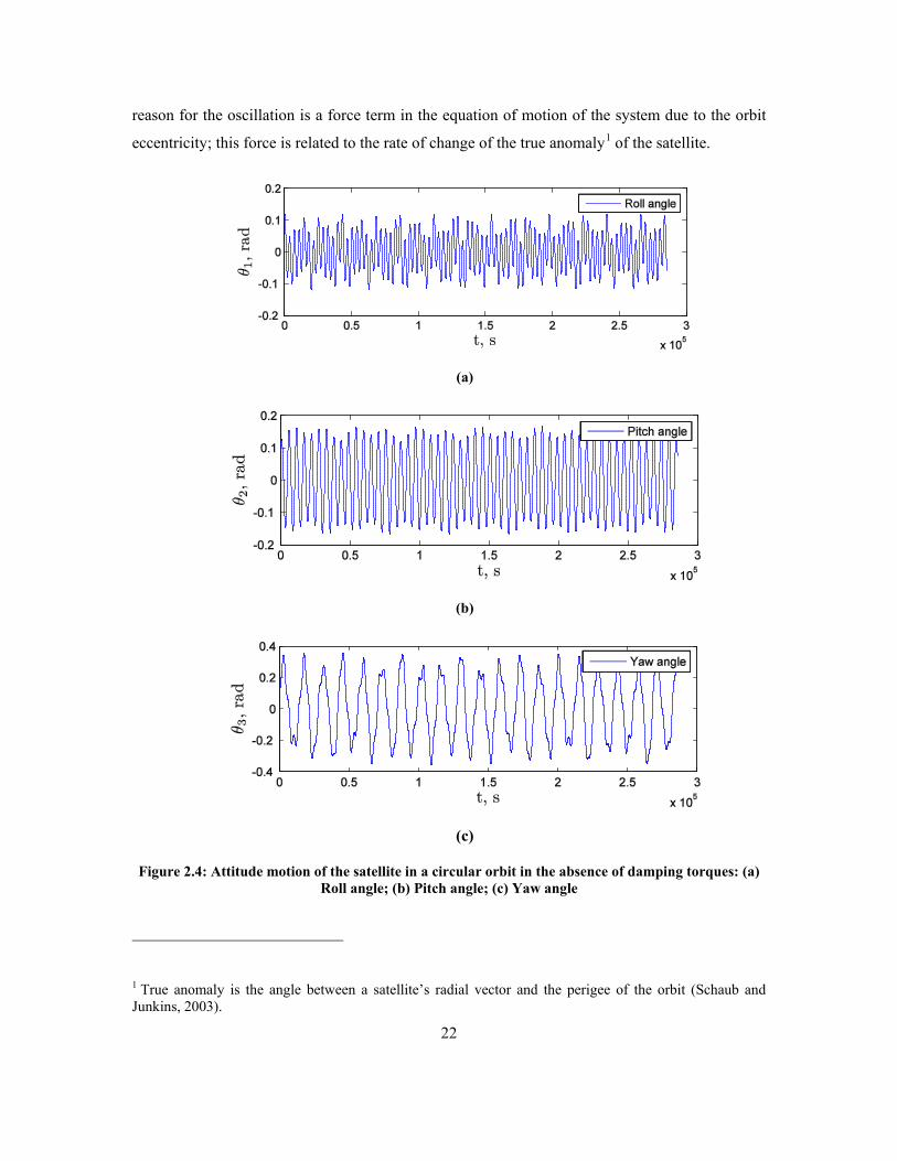
reason for the oscillation is a force term in the equation of motion of the system due to the orbit

eccentricity; this force is related to the rate of change of the true anomaly1 of the satellite.

(a)

(b)

(c)

Figure 2.4: Attitude motion of the satellite in a circular orbit in the absence of damping torques: (a) Roll angle; (b) Pitch angle; (c) Yaw angle

1 True anomaly is the angle between a satellite’s radial vector and the perigee of the orbit (Schaub and Junkins, 2003).

22

(a)

(b)

(c)

Figure 2.5: Attitude motion of a satellite in an elliptical orbit with the eccentricity of 0.05 in the absence of damping torques: (a) Roll angle; (b) Pitch angle; (c) Yaw angle

23

(a)

(b)

(c)

Figure 2.6: Attitude motion of the satellite in a circular orbit in the presence of damping torques of four fluid rings: (a) Roll angle; (b) Pitch angle; (c) Yaw angle

24

(a)

(b)

(c)

Figure 2.7: Attitude motion of a satellite in an elliptical orbit with the eccentricity of 0.05 in the presence of damping torques of four fluid rings: (a) Roll angle; (b) Pitch angle; (c) Yaw angle

The effect of the pyramidal configuration angles on the damping torque is investigated next.

To this end, the angle 𝛾 is varied from a value slightly more than 0° to slightly less than 90°.

Figures 2.6-2.8 correspond to the cases where the angle 𝛼 is 45°, and the angle 𝛾 being chosen as

25

5°, 45°, and 85°. It can be seen that upon increasing the angle 𝛾, a larger damping torque can be

obtained. However, the damping effect is still not fast enough (the reduction of the satellite

attitude angles is about 70% of their initial values in 50 orbits) even for large values of 𝛾 .

Therefore, a controller is required for both circular and elliptical cases.

(a)

(b)

(c)

Figure 2.8: Attitude angles for the pyramidal angle 𝛾 = 5°: (a) Roll angle; (b) Pitch angle; (c) Yaw angle

(a)

(b)

26

(c)

Figure 2.9: Attitude angles for the pyramidal angle 𝛾 = 45°: (a) Roll angle; (b) Pitch angle; (c) Yaw angle

(a)

(b)

(c)

Figure 2.10: Attitude angles for the pyramidal angle𝛾 = 85°: (a) Roll angle; (b) Pitch angle; (c) Yaw angle

Finally, for the reader’s quick reference, the results of analyzing the stability condition of

satellites in both circular and elliptical orbits, with and without fluid rings, are summarized in

Tables 2.1 and 2.2.

27

Table 2.1: Stability condition of a satellite in a circular orbit

Attitude angle Without fluid rings With passive fluid rings

Stability condition Stabilization

time

Stability condition Stabilization

time

Roll Stable (limit cycle) N/A Asymptotically

stable

More than 50

orbits

Pitch Stable (limit cycle) N/A Asymptotically

stable

More than 50

orbits

Yaw Stable (limit cycle) N/A Asymptotically

stable

More than 50

orbits

Table 2.2: Stability condition of a satellite in an elliptical orbit with the eccentricity of 0.05

Attitude angle Without fluid rings With passive fluid rings

Stability condition Stabilization

time

Stability condition Stabilization

time

Roll Stable (limit cycle) N/A Asymptotically

stable

More than 50

orbits

Pitch Stable (limit cycle) N/A Stable (limit cycle) N/A

Yaw Stable (limit cycle) N/A Asymptotically

stable

More than 50

orbits

28

2.4 Summary

In this chapter, the dynamical model of a rigid satellite with fluid ring actuators was

developed. The model is obtained for two satellites: one with three orthogonal fluid rings; the

other with four in a pyramidal configuration. The passive damping effect of the fluid rings on the

satellite attitude angles was examined. It was noted that the damping torque of the fluid rings was

neither large enough to eliminate the oscillations of the satellite within a short period of time, nor

could asymptotically stabilize the pitch angle of a satellite in an elliptical orbit. Further, the effect

of the pyramidal configuration angle on the damping torque was investigated. The result showed

that, although a larger pyramidal configuration angle increases the damping effect, the decay

process is still quite slow. Hence, designing an active controller is necessary.

29

30

Chapter 3

DESIGNING OF CONTROLLERS FOR SATELLITES

WITH FLUID RINGS

The dynamical model of a satellite with fluid ring actuators was developed in Chapter 2. The

results obtained from this model showed that designing an active controller for fast asymptotic

stabilization of the attitude motion is essential; this is thoroughly discussed in this chapter.

In this vein, as the first attempt, a PID controller is designed to examine the behaviour of the

fluidic actuators. The case of failure of one fluid ring is also studied so as to test the redundancy

of the system with four fluid rings in a pyramidal configuration.

A PID controller, whose gains are adjusted offline, relies heavily on the accuracy of the

dynamical model. However, there are always uncertainties in a dynamical model associated with

different components, such as sensors, actuators, etc. In fact, a robust controller is required to

cope with the inevitable error in the fluid model as well as the uncertainties in the system

parameters. A sliding mode controller, which can be applied to nonlinear systems, is an

appropriate candidate. Therefore, a sliding mode controller is designed in this chapter, whose

performance is found to be quite promising.

31

3.1 PID Controller

Deriving the equations of motion of the satellite with fluid rings actuators, the objective here

is to stabilize the system at its equilibrium state, where we have:

𝛚� = [0 −1 0]T, 𝛽𝑖′ = 0, 𝜽 = 𝟎 (3. 1)

in which 𝜽 = [𝜃1 𝜃2 𝜃3]𝑇 , 𝜃𝑖 for 𝑖 = 1, … ,3 being the roll, pitch, and yaw angles,

respectively1. Adding the control input to the equations of motion of the satellite and the fluid

rings, Eqs. (2.21) and (2.22), yields

𝑰�𝒔𝝎�′ + 𝝎� × 𝑰�𝒔𝝎� = 𝝉�𝒈𝒈 + ∑ 𝑹𝒊𝝉�𝒓𝒊𝒌𝒊=𝟏 + 𝝉�𝒄 for 𝑘 = 3 or 4 (3. 2)

𝑰�𝒇𝒊�𝑹𝒊𝑻𝝎�′ + 𝜷𝒊′′ + 𝑹𝒊𝑻𝝎� × 𝜷𝒊′� + 𝑹𝒊𝑻𝝎� × 𝑰�𝑓𝑖�𝑹𝒊𝑻𝝎� + 𝜷𝒊′� = 𝑹𝒊𝑻𝝉�𝒈𝒈𝒇𝒊 − 𝝉�𝒓𝒊 − 𝝉�i𝒄 (3. 3)

where 𝝉�𝒄 is produced by the pumps that pressurize the fluid inside the rings, 𝝉�i𝒄 being the

component of 𝝉�𝒄 that has to be produced by the 𝑖th fluid ring.

To apply a PID controller, in Eqs. (3. 2) and (3. 3), 𝝉�𝒄 is replaced by the PID control law

given below:

𝝉�𝒄 = 𝐾𝑝(𝜽 − 𝜽𝒅) + 𝐾𝑑(𝜽′ − 𝜽′𝒅) + 𝐾𝑖 �� 𝜽 𝑑Γ𝑇

0− � 𝜽𝒅 𝑑Γ

𝑇

0 � (3. 4)

where 𝑇 and Γ are the non-dimensional time variables. Figures 3.1−3.3 show the simulation

results obtained after implementing the PID controller in a satellite with four fluid rings in a

pyramidal configuration. The non-dimensional system parameters and initial conditions are

chosen identical to the ones introduced in Section 2.3. Also, the satellite is assumed to be in a

circular orbit with the radius of 7000 km as in Chapter 2. Figure 3.1 shows that the satellite

attitude angles are asymptotically stabilized at their equilibrium state in less than five minutes. As

1 The notation used throughout the whole thesis is uniform. A nomenclature section is added at page xi for quick reference.

32

can be seen in Figure 3.2, the maximum torque required is less than 0.015 N. m. To produce this

torque, the maximum fluid angular velocity required is 7 rad/s (Figure 3.3).

(a)

(b)

(c)

Figure 3.1: Attitude angles of the controlled system with PID gains 𝐾𝑝 = 5000, 𝐾𝑑 = 10, and 𝐾𝑖 = 0.5 (circular orbit): (a) Roll angle; (b) Pitch angle; (c) Yaw angle

33

(a)

(b)

(c)

Figure 3.2: Control torque components with PID gains 𝐾𝑝 = 5000, 𝐾𝑑 = 10, and 𝐾𝑖 = 0.5 (circular orbit case); (a) Roll angle; (b) Pitch angle; (c) Yaw angle

34

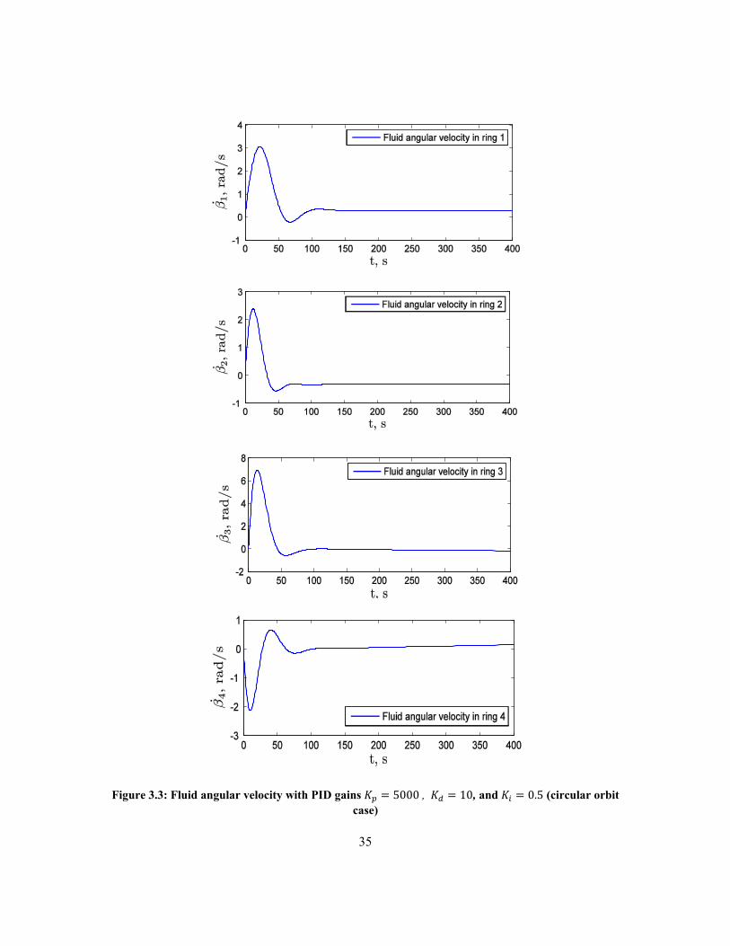
Figure 3.3: Fluid angular velocity with PID gains 𝐾𝑝 = 5000 , 𝐾𝑑 = 10, and 𝐾𝑖 = 0.5 (circular orbit case)

35

It is also interesting to determine the effect of varying the angle 𝛾 shown in Figure 2.2, on

the performance of the active controller. To this end, simulation was carried out by considering

different values of 𝛾, let say 5°, 45°, and 85°, respectively. The results are presented in Figures

3.4 and 3.5.

(a)

(b)

(c)

Figure 3.4: Attitude angles of the controlled system with various pyramidal angles using PID gains 𝐾𝑝 = 5000 , 𝐾𝑑 = 10, and 𝐾𝑖 = 0.5 (circular orbit case): (a) 𝛾 = 5°; (b) 𝛾 = 45°; (c)

𝛾 = 85°

36

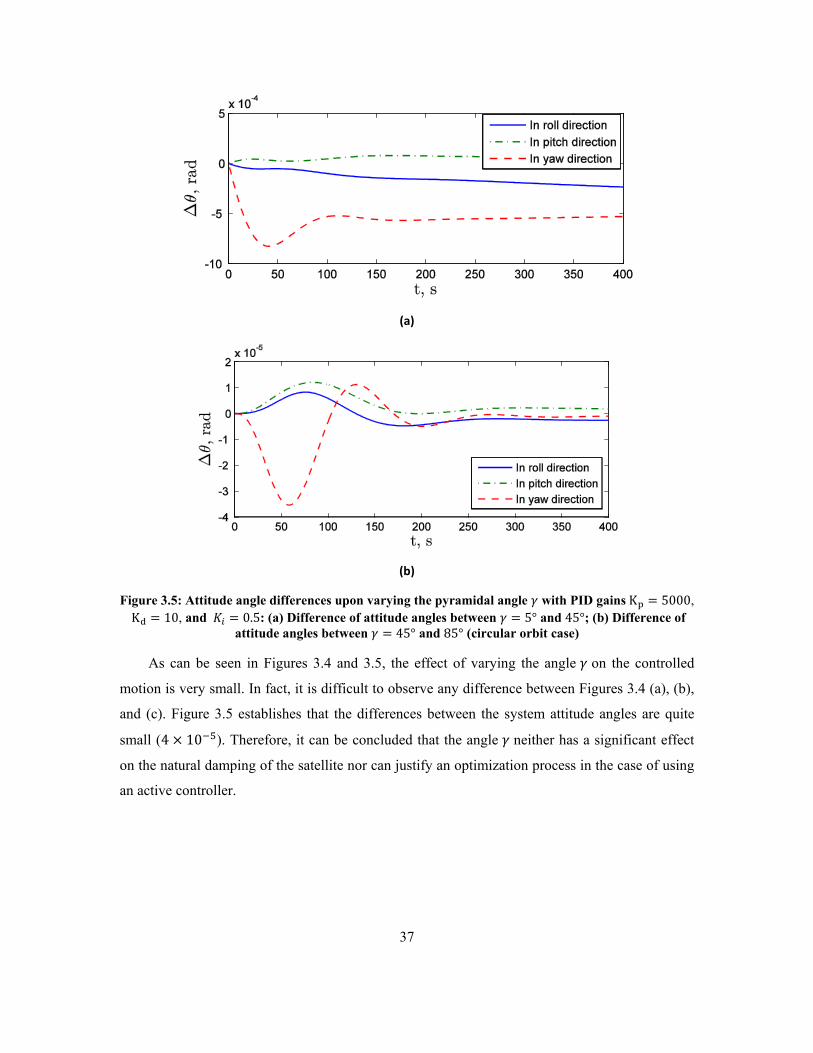
(a)

(b)

Figure 3.5: Attitude angle differences upon varying the pyramidal angle 𝛾 with PID gains Kp = 5000, Kd = 10, and 𝐾𝑖 = 0.5: (a) Difference of attitude angles between 𝛾 = 5° and 45°; (b) Difference of

attitude angles between 𝛾 = 45° and 85° (circular orbit case)

As can be seen in Figures 3.4 and 3.5, the effect of varying the angle 𝛾 on the controlled

motion is very small. In fact, it is difficult to observe any difference between Figures 3.4 (a), (b),

and (c). Figure 3.5 establishes that the differences between the system attitude angles are quite

small (4 × 10−5). Therefore, it can be concluded that the angle 𝛾 neither has a significant effect

on the natural damping of the satellite nor can justify an optimization process in the case of using

an active controller.

37

3.2. Failure Analysis

Due to the sensitivity of satellite operations, the possibility of failure of control actuators

cannot be neglected. Accordingly, for the control system proposed, the case of failure of one fluid

ring is examined here. In fact, having four fluid rings adds redundancy to the system. Thus, with

one fluid ring failed, while the other three are functional, the satellite attitude angles can still be

stabilized at its equilibrium state upon re-tuning the PID gains. The simulation is done for four

different cases associated with the failure of each of the four fluid rings. Based on the results

obtained, two main points are concluded: (i) the fact that which fluid ring has failed does not

make a significant difference in the attitude motion of the satellite. Thus, for the sake of brevity in

Figure 3.6, a fluid ring is arbitrarily selected to be considered as failed; (ii) it was noted that the

fluid flow inside the rings, as shown in Figure 3.6 (b) and (c), does not eventually vanish,

although the total torque produced is zero. This implies that

∑ 𝝉𝒋𝒄4𝑗=1 = 0, 𝝉𝒋 ≠ 𝟎 for 𝑖 = 1, … ,4 (3. 5)

In fact, Figure 3.6 (b) shows that the angular velocity of the fluid continuously increases,

however with a quite small rate. This is not acceptable since pumping fluid consumes the

valuable power resources. Further, the fluid rings will finally be saturated, meaning that, at some

point, the pumps will reach their limits and cannot increase the fluid angular velocity any further

because of the existing friction. Once the saturation of the fluid rings occurs, the satellite attitude

motion cannot be stabilized. To cope with this problem, the original PID controller is modified, as

per the equation below, by adding a weighted summation of the fluid angular velocity terms:

𝝉�𝒄 = 𝐾𝑝(𝜽 − 𝜽𝒅) + 𝐾𝑑(𝜽′ − 𝜽′𝒅) + 𝐾𝑖 �� 𝜽 𝑑𝛤𝑇

0− � 𝜽𝒅 𝑑𝛤

𝑇

0 �

+𝐾𝑣(𝑹𝟏𝑻𝜷𝟏′ + 𝑹𝟐𝑻𝜷𝟐′ + 𝑹𝟑𝑻𝜷𝟑′ + 𝑹𝟒𝑻𝜷𝟒′ )

(3. 6)

38

(a)

(b)

(c)

Figure 3.6: Response of the system subject to the failure of one fluid ring with using PID gains 𝐾𝑝 = 5000 , 𝐾𝑑 = 10, and 𝐾𝑖 = 0.5 (circular orbit case): (a) Satellite attitude angles; (b) Fluid

angular velocity in the rings; (c) Resultant control torque

39

Choosing an appropriate value for the gain 𝐾𝑣 in Eq. (3. 6), the response of the system is

plotted in Figure 3.7. Given this provision, not only the satellite attitude angles are stabilized in a

short time period, about 300 s, but also the fluid angular velocities vanish in the steady response.

It is noteworthy that the maximum torque produced is about 0.01 N. m; to produce this amount of

torque, the fluid angular velocity required is less than 7 rad/s.

(a)

(b)

(c)

Figure 3.7: Response of the system associated with the failure of one fluid ring using the gains 𝐾𝑝 = 5000 , 𝐾𝑑 = 10, 𝐾𝑖 = 0.5, and 𝐾𝑣 = −0.5 (circular orbit case): (a) Satellite attitude angles; (b)

Fluid angular velocity in the rings; (c) Control torque

40

3.3. Designing a Sliding Mode Controller

One important factor to consider in designing a controller is its robustness. The importance

of this factor becomes more apparent, if the uncertainty in the model itself and also in the system

parameters is recalled. A sliding mode controller, which is applicable to nonlinear models, is

robust against parametric uncertainties. There is an extensive literature on attitude control of

satellites using sliding mode controllers, but only a few focuses on attitude stabilization using

reaction/momentum wheels, which closely resemble the fluid ring actuators. For instance, for a

satellite equipped with thrusters and reaction wheels, Topland and Gravdahl (2004) compared a

sliding mode controller to three other alternatives. They concluded that the sliding mode

controller, although not the optimum option, is capable of tolerating high levels of model

uncertainties. Terui et al. (2005) designed a sliding mode controller for a moon-tracking satellite.

The system considered included two momentum wheels for three-dimensional attitude

stabilization. Ashrafiuon and Erwin (2005) studied a satellite with a single reaction wheel. They

proposed a scheme to change the moment of inertia and angular velocity of the wheel to conserve

the angular momentum of the system. They chose a sliding mode controller to cope with the

nonlinearity of the system and also to add robustness to its performance. Kowalchuk and Hall

(2008) proposed a new method to develop a sliding mode control law for a satellite with reaction

wheels; the performance of the controller was tested via a hardware-in-the-loop experiment.

Recently, Huo et al. (2011) implemented a sliding mode controller in a tracking satellite with

reaction wheels; an adaptive controller was also used to estimate the upper bound of external

disturbances.

Our aim here is to develop a sliding mode controller to stabilize the satellite attitude angles

using the nonlinear model developed. In this case, because the goal is to stabilize the system on

zero attitude angles, the following sliding hypersurface 1 is assumed (Slotine and Weiping, 1991):

𝑠𝑖 = 𝜃𝑖′ + 𝜆𝜃𝑖 for 𝑖 = 1, … ,3 (3.7)

1 In sliding mode control design, the command should force the states of the system to move (slide) along the boundaries of a specific control structure, which is called the sliding hypersurface (Slotine and Weiping, 1991).

41

where 𝑠𝑖 is the sliding surface for the 𝑖th angle, and 𝜃𝑖′ is the non-dimensional attitude angle

derivative. The parameter λ is the slope of the line chosen as the hypersurface here. Large values

of 𝜆 result in a faster stabilization at the cost of consuming more power. The attitude stabilization

can be achieved when 𝜃𝑖′ and 𝜃𝑖 are zero, which in turn implies that at the equilibrium 𝑠𝑖 is

required to vanish. As an instance, the sliding line used for controlling the roll angle of the

satellite understudy is shown in Figure 3.8.

Figure 3.8: Sliding hypersurface for the roll direction

In order to proceed, an initial estimate of the parameters of the system, henceforth referred to

as their nominal values, is required. Prior to designing the sliding mode controller, a notation

convention needs to be established here: a parameter with an overhead bar denotes its nominal

value, while without an overhead bar designates its actual value.

Generally speaking, the sliding mode control law has the following form (Slotine and

Weiping, 1991):

𝝉�𝒄 = �̅�(𝒖� − 𝒌 𝑠𝑔𝑛(𝑠)) (3. 8)

where �̅� is a modified inertia matrix, 𝒌 being a design parameter vector; these two terms will be

discussed shortly. Further, 𝒖� is a vector resulting from the addition of the derivative of the

sliding surfaces vector with respect to time to a vector denoted by 𝒈�, whose components are the

variables of interest to be controlled. In attitude stabilization problem, 𝒖� can be expressed as:

𝒖� = 𝒈� + [s1′ s2′ s3′ ]T (3. 9)

Sliding slope 𝜆

42

where 𝒈� ≡ 𝝎′. Substituting 𝑠𝑖 from Eq. (3.7) into Eq. (3. 9), 𝒖� can be found as:

𝒖� = 𝒈� + 𝜽𝒅′′ − 𝜆𝜽′ (3.10)

To find 𝒈�, first, Eqs. (2.11) and (2.12) should be substituted into Eq. (2.2) in order to find the

equation of motion of the satellite free of the fluid angular acceleration terms:

�𝑰�𝒔 + �𝑹𝒊𝑬𝑰�𝒇𝒊𝑹𝒊𝑻𝑘

𝑖=1

�𝝎′ + 𝝎� × 𝑰�𝒔𝝎� = 𝝉𝒈𝒈 + �𝑹𝒊𝑬𝑹𝒊𝑻𝝉𝒈𝒈𝒇𝒊

𝑘

𝑖=1

−�𝑹𝒊𝑬{𝑰�𝒇𝒊�𝑹𝒊𝑻𝝎� × 𝜷𝒊′� + 𝑹𝒊𝑻𝝎� × 𝑰�𝒇𝒊�𝑹𝒊𝑻𝝎� + 𝜷𝒊′�𝑘

𝑖=1

} + �𝑹𝒊[0 0 𝜏𝑓𝑖]𝑇𝑘

𝑖=1

(3.11)

Here, 𝑬 = [𝒆𝟏 𝒆𝟐 𝟎]𝑻 with 𝒆𝟏 = [1 0 0]𝑇, 𝒆𝟐 = [0 1 0]𝑇. Now, 𝒈� is defined as:

𝒈� ≡ 𝝎′ = 𝑱−𝟏(−𝝎� × 𝑰�𝒔𝝎� + 𝝉�𝒈𝒈 + �𝑹�𝒊𝑬𝑹�𝒊𝑻𝝉�𝒈𝒈𝒇𝒊

𝑘

𝑖=1

−�𝑹�𝒊𝑬{𝑰�𝒇𝒊�𝑹�𝒊𝑻𝝎� × 𝜷𝒊′� + 𝑹�𝒊𝑻𝝎� × 𝑰�𝒇𝒊�𝑹�𝒊𝑻𝝎� + 𝜷𝒊′�𝑘

𝑖=1

} + �𝑹�𝒊[0 0 𝜏�̅�𝑖]𝑇𝑘

𝑖=1

)

(3.12)

The term �̅� is the modified inertia matrix that also appeared in Eq. (3.8). This matrix is indeed the

coefficient of 𝝎′ in Eq. (3.11):

�̅� = 𝑰�𝒔 + �𝑹�𝒊𝑬𝑰�𝒇𝒊𝑹�𝒊𝑻4

𝑖=1

(3.13)

The only term remaining in Eq. (3.8) to be defined is the vector 𝒌. According to Slotine and

Weiping (1991),

𝒌 = �𝐹1 + 𝜂1𝐹2 + 𝜂2𝐹3 + 𝜂3

� (3.14)

43

where 𝜂𝑖 for 𝑖 = 1, … ,3 are the control design variables to be tuned. In order to introduce 𝐹𝑖 for

𝑖 = 1, … ,3, first, the inequality below is recalled from (Slotine and Weiping, 1991):

‖𝒈� − 𝒈‖ ≤ �[F1 F2 F3]T� (3.15)

where ‖. ‖ denotes the 2-norm of a vector. Equation (3.15) states that 𝑭 = [F1 F2 F3]T is a

vector to be defined such that its 2-norm is greater than that of the vector (𝒈� − 𝒈) , which

measures the difference between the nominal and actual angular accelerations of the satellite in

the problem at hand. Here, 𝐹𝑖 is chosen as:

𝐹𝑖 = 16𝜋𝑎�1𝑎�2�̅� ��𝛽𝑖′2

k

𝑖=1

�

1/2

(3.16)

The reason behind this choice is that, in sliding mode control design, it is advised to select a

physically meaningful quantity to be used as 𝐹𝑖 variable; the non-dimensional fluid friction torque

is hence chosen in Eq. (3.16). To investigate the performance of the sliding mode controller on

the system, simulations are performed; the results are presented in the next subsection.

3.3.1. Dynamical behaviour of the system with the sliding mode controller

To study the performance of the sliding mode controller designed in the preceding section, a

satellite with the nominal parameters identical to the non-dimensional parameters of the satellite

introduced in Section 2.3 is considered; the parameters are assumed to have an uncertainty of

±15%. Using the same initial conditions and orbital radius as those given in Section 2.3, the

attitude angle variations of the satellite are plotted versus time in Figure 3.9. It can be concluded

that despite the quite large uncertainty in the system parameters, the controller can satisfactorily

stabilize the satellite attitude angles in about 500 𝑠.

Figure 3.9: Attitude angles after applying the sliding mode controller (circular orbit case)

44

(a)

(b)

(c)

Figure 3.10: Components of the control torque resulting from the sliding mode controller: (a) Roll direction; (b) Pitch direction; (c) Yaw direction (circular orbit case)

Figure 3.10 shows the three components of the control torque produced by the sliding mode

controller in the roll, pitch, and yaw directions. As can be seen, a high-frequency chattering exists

after the transient response has been eliminated; this phenomenon is a well known characteristic

of sliding mode controllers. Several methods have been proposed in the literature to modify the

45

control law to reduce this effect. In the next section, a switching control law is proposed to

eliminate the chattering effect.

3.4. Switching Control Law

In order to eliminate the chattering in the response of the sliding mode controller designed in

the foregoing section, a switching controller combining a PID with the sliding mode controller is

set forth. The idea is to use the sliding mode controller until the error, 𝛿 = ‖𝜽 − 𝜽𝒅‖ becomes

small enough, i.e., 𝛿 ≤ 𝜀, where 𝜀 is a small number; at this point, the sliding mode control law

is replaced by a PID controller to asymptotically stabilize the satellite attitude angles. In the

general form, the control law for the switching controller can be written as:

�𝝉�𝒄 = �̅��𝒖� − 𝒌 𝑠𝑔𝑛(𝑠)� 𝛿 > 𝜀

𝝉�𝒄 = 𝐾𝑝(𝜽 − 𝜽𝒅) + 𝐾𝑑(𝜽′ − 𝜽′𝒅) + 𝐾𝑖 �� 𝜽 𝑑Γ𝑇

0− � 𝜽𝒅 𝑑Γ

𝑇

0 � 𝛿 ≤ 𝜀

� (3. 17)

Figure 3.11: Attitude angles after applying the switching controller (circular orbit case)

Designing the switching controller for the satellite studied in Subsection 3.3.1, the variation

of the attitude angles are illustrated in Figure 3.11, the control torque components being shown in

Figure 3.12. At 𝑡 = 578 s, the switching controller switches to the PID controller; the value of ε

used here is 5 × 10−3 . As can be noticed in Figure 3.12, the chattering in the control input has

been eliminated after this time step. The maximum control torque required is about 0.6 N. m in

the roll direction, which is fairly high.

It is also interesting to compare these results to the case, in which a PID controller is only

used. To this end, a PID controller is tuned for the satellite with the nominal parameter values.

The attitude motion of this system is shown in Figure 3.13. Further, using the same PID gains, the

46

attitude angle variations are plotted in Figure 3.14, this time considering the 15% uncertainty of

the parameters. It can be concluded from the two figures that the PID controller is not robust

enough to be capable of properly handling a ±15% uncertainty in the parameter values. Despite

this fact, for the purpose of the feasibility analysis of using fluid ring actuator in satellites, PID

controllers will be designed in the forthcoming chapters.

(a)

(b)

(c)

Figure 3.12: Control torque resulting from the switching controller; (a) Roll direction; (b) Pitch direction; (c) Yaw direction (circular orbit case)

47

Figure 3.13: Satellite attitude angles using a PID controller with the nominal parameter values

Figure 3.14: Satellite attitude angles using a PID controller subject to the ±15% uncertainty in the nominal parameter values

3.5. Summary

In this chapter, a PID controller was designed to demonstrate the feasibility of attitude

stabilization of a satellite with fluid rings. The advantage of using a redundant set of fluid rings

was also discussed by performing a failure analysis. To cope with the uncertainty of the

dynamical model parameters, a sliding mode control law was also developed. The chattering in

the steady response of the system, that is a well-known characteristic of sliding mode controllers,

was eliminated via designing a switching controller consisting of a sliding mode and a PID

controller. The simulation results showed that the attitude angles were asymptotically stabilized

in less than 500 𝑠, although a fairly high control torque, about 0.6 N. m, was required.

48

Chapter 4

EXPERIMENTAL RESULTS

In this chapter, the theoretical results reported in Chapters 2 and 3 are validated by

conducting several experiments. To this end, initially, a setup with one fluid ring is designed and

built. A few preliminary tests are then conducted to find a relation between the input voltage and

the fluid angular velocity. Next, experiments are conducted to verify if the fluid ring is capable of

producing a large enough torque to control the attitude of a satellite. A setup consisting of three

orthogonal fluid rings is then used to evaluate the three-dimensional control algorithm. The

experiments reported in this chapter are done in collaboration with a team from Ryerson

University. The setup used in the experiments, reported in this chapter, was designed and built at

Ryerson University. However, the design of the experiments, data processing and the analysis of

the experimental results are solely performed by the author in her course of doctoral research.

4.1. Design of the Experimental Setup

The main component of the experimental setup is the fluid ring. Here, the selection of an

appropriate fluid, a material for the structure of the ring, and a pump are among the major issues,

49

which are to be discussed in more detail. It is noteworthy that the preference is to choose the

components and materials, which are space qualified. However, this is not a concern for the

experimental setup meant to validate the feasibility of using fluid ring actuators.

4.1.1. Material selection

Metals are suitable candidates for the structure of the rings, as opposed to plastics, which are

not durable enough in the low and high temperature and low pressure of the space. The ease of

machining and soldering, electrical insulation, and low mass density are the most significant

properties to be considered while choosing a proper metal. Among these, the machining

simplicity is highly important, since the size of the rings is quite small. With this regard, copper

and aluminum are appropriate options. Comparing the two, an aluminum ring has a smaller mass

with lower electrical conductivity, but cannot be soldered easily. Therefore, to build a circular

ring, the aluminum tube should be shrink-fitted, a process that is quite costly, at least, for the

experimental stage. Knowing this fact and also taking a hint from the condenser systems in

satellites, copper is chosen as the superior alternative to build the loop of the fluid ring setup in

the experiments.

4.1.2. Fluid selection

To select an appropriate fluid, the properties such as the boiling and freezing points,

viscosity, density, and toxicity should be taken into account. The importance of each property is

described below.

i. Boiling and freezing points: the variation of temperature is quite significant in space.

Hence, the number of possible choices for a fluid type is limited, since it is essential that

the fluid maintains its state during the whole operation.

ii. Viscosity: in Chapter 2, it was shown that the friction torque resulting from the viscosity

can damp out the attitude oscillations of a gravity gradient stabilized satellite. However,

if the fluid is highly viscous, the pump cannot easily produce the flow. Indeed, the high

friction torque reduces the efficiency of the active fluidic actuator. This is due to the fact

that the torque produced by the pump is in opposite direction to the friction torque

produced by the viscosity.

50

iii. Density: the higher the moment of inertia of the fluid, the larger the torque that the fluid

ring produces. Indeed, the moment of inertia of the fluid is directly proportional to its

density.

iv. Toxicity: the fluid should not impose any risk to the health of the researchers.

v. Corrosive: the fluid chosen should not be corrosive; otherwise it can damage the pump.

The first item above eliminates many fluid types from the selection list. Indeed, antifreezes

and refrigerators’ working fluids are good options considering the thermal variations, which is

common in space. Of these types, Freon and Ammonia are commonly utilized in capillary

pumped loops; also, Ethylene and Propylene glycol are antifreeze fluids in vehicles. The

properties of these fluids are summarized in Table 4.1. From the table, it can be understood that

the glycols maintain their liquid phase in a larger thermal interval. Comparing ethylene glycol

and propylene glycol, the former is finally chosen for its higher density.

Table 4.1: Fluid properties

Fluid Viscosity, P𝑎. 𝑠

At 20℃

Density, 𝐾𝑔/𝑚3

At 20℃

Pressure, 𝐴𝑡𝑚

At 20℃

Freezing point,

℃

Boiling point,

℃

Water 0.823 997 1 0 100

Ammonia 1.5 × 10−4 600 8.39 −78 −33.5

Freon-11 0.004 1494 1 −111.1 23.8

Freon-12 0.002 1329 5.58 −157.7 −29.75

Ethylene Glycol 0.060 1095 1 −46.63 187.4

Propylene Glycol 0.090 1045 1 −45.5 197.1

4.1.3. Pump selection

The requirements of the system affecting the pump selection are categorized into two groups

of primary and secondary. The primary requirements relate to the capacity of the pumps in order

to produce a high flow rate in low pressure conditions, while operating with a DC voltage. On the

other hand, the mass and the size of the pump, its compatibility with the metal loop, and its

operation life are among the secondary requirements.

51

Among various types available, reciprocating pumps have pulsed operation and cannot thus

produce a continuous flow. Hence, they are not appropriate for our application. Diaphragm

pumps can operate in low pressure but cannot produce a high flow rate. Centrifugal pumps

produce continuous high flow rates, even at low pressure. As centrifugal pumps, which can

operate with a DC voltage exist, this type of pumps is chosen to be used in the experimental

setup. Considering the secondary requirements, like the size of the pump, TCS-M400 which is

designed and manufactured by TCS Micro Pumps, is chosen. This pump is a small, low mass

centrifugal pump, which is available in the market.

Figure 4.1 shows a fluid ring built for the experiments. The ring is made of copper and

equipped with a TCS-M400 centrifugal pump. The cross-sectional diameter of the ring is 9 mm,

its radius is 8 𝑐𝑚 so as to fit within a 20 cm cube. The ring is filled with ethylene glycol, as

discussed earlier; the moment of inertia of the fluid about the axis of symmetry of the ring is

4.54 × 10−4 kgm2. Further, the plastic base holder has a moment of inertia of 5.37 × 10−2 kgm2

about the same axis.

Figure 4.1: The fluid ring used in the experimental validation phase

4.2. Preliminary Analysis

To perform the experiments, first, a relation between the fluid rate and the voltage applied to

the pump is required. To this end, the angular velocity of the impeller 𝜔𝑖𝑚𝑝 is measured versus

TCS-M400

centrifugal pump

52

the applied voltage 𝑉𝑎𝑝𝑝; the resulting data are plotted in Figure 4.2. Using the least square fit, the

equation below is found between 𝜔𝑖𝑚𝑝 and 𝑉𝑎𝑝𝑝:

𝜔𝑖𝑚𝑝 = 0.682 Vapp + 1.836 (4.1)

Figure 4.2: Angular velocity of the impeller versus the applied voltage

Next, before finding the relation between the input voltage and the angular velocity of the

fluid �̇� inside the ring, a relation between the latter and the angular velocity of the impeller is

obtained. To this end, an experiment is conducted in which one fluid ring is mounted on a

simulator that maintains the fluid ring floating in the air (Figure 4.3). The simulator is equipped

with a gyroscope to find the angular velocity of the setup.

In the experiment, the following sinusoidal voltage was applied to the pump:

𝑉𝑎𝑝𝑝 = �8 𝑡 < 30𝑠8 + 3 sin(0.1𝜋𝑡) 𝑡 ≥ 30𝑠

� (4.2)

where 𝑡 denotes the time. According to Eq. (4.2), a voltage of 8 V is applied at the first 30 s of the

experiment so as to allow the operator to initialize the angular velocity of the setup at 0 rad/s.

After 𝑡 = 30 s, the sinusoidal input voltage is applied; the angular velocity of the base and the

ring are measured using the gyroscope, while the impeller angular velocity was found using an

encoder. The angular velocity of the fluid versus the angular velocity of the impeller is plotted in

Figure 4.4.

53

Figure 4.3: Fluid ring with its base mounted on the simulator

Figure 4.4: Fluid angular velocity �̇� versus the impeller angular velocity 𝜔𝑖𝑚𝑝 using a sinusoidal input voltage

Using the least square fit, the following relation between �̇� and 𝜔𝑖𝑚𝑝 can be found:

�̇� = 0.11𝜔𝑖𝑚𝑝 − 0.11 (4.3)

Combining Eqs. (4.1) and (4.3), the relation sought between the input voltage and the fluid

angular velocity �̇� is obtained as:

54

�̇� = 0.08Vapp + 0.10 (4.4)

Using this equation, the voltage required to produce the desired fluid angular velocity can be

calculated.

4.3. Experiment with a Single Fluid Ring System

In this experiment, the target is to verify if:

i. the system with a fluid ring is controllable.

ii. the theoretical model represents the real fluid ring behaviour within acceptable precision.

iii. a fluid ring is capable of producing a large enough control torque.

To this end, the equations of motion of the system, i.e., a single fluid ring mounted on its base, as

shown in Figure 4.3, are first derived.

𝐼𝑏�̈� = 𝜏𝑎 , 𝐼𝑓��̈� + 𝛽�̈�� = −𝜏𝑎 (4.5)

Here, 𝜃 is the attitude angle of the disk about its axis of symmetry; �̈�𝑑 is the desired fluid angular

acceleration; 𝐼𝑏 and 𝐼𝑓 are the moments of inertia of the base and the fluid inside the ring about

the axis of symmetry of the disk. Further, 𝜏𝑎 is the torque that the fluid ring applies on the base.

In fact, the torque 𝜏𝑎 has two components:

𝜏𝑎 = 𝜏𝑓 + 𝜏𝑝 (4.6)

where 𝜏𝑓 and 𝜏𝑝 are the fluid friction torque and the torque resulting from the pump pressure,

respectively. To control the system, the pump pressure torque is found using a PD control law:

𝜏𝑝 = 𝐾𝑝(𝜃 − 𝜃𝑑) + 𝐾𝑑��̇� − �̇�𝑑� (4.7)

where 𝜃𝑑 is the desired attitude angle chosen arbitrarily. To better demonstrate the different

components involved in the control of the system at hand and their relations, a block diagram of

the whole process is illustrated in Figure 4.5. In fact, in order to stabilize the system at the attitude

angle 𝜃𝑑, the PD control law (4.7) is substituted into Eq. (4.5), thereby the desired fluid angular

55

velocity �̇�𝑑 and acceleration �̈�𝑑 are obtained. Since the actual control input is the voltage 𝑉𝑐 to be

supplied to the pump, a PD control law is designed below so as to produce the flow rate �̇�𝑑.

𝑉𝑐 = 𝑉𝑎𝑝𝑝 + 𝐾𝑝�𝜔𝑖𝑚𝑝 − 𝜔𝑖𝑚𝑝𝑑� + 𝐾𝑑��̇�𝑖𝑚𝑝 − �̇�𝑖𝑚𝑝𝑑� (4.8)

In the preceding equation, 𝑉𝑎𝑝𝑝 can be obtained upon substituting �̇�𝑑 into Eq. (4.4), 𝜔𝑖𝑚𝑝𝑑 and

�̇�𝑖𝑚𝑝𝑑 being the desired angular velocity and acceleration of the impeller.

In our experimental setup, the data and the control commands are transmitted between the

system and the computer via radio signals. Therefore, for a more reliable performance, a filter is

required to eliminate the noise from the measured data; this is discussed next.

Figure 4.5: The block diagram of the controllers used between the model and the plant

4.3.1. Designing a Kalman filter

A discrete Kalman filter uses the data measured by sensors from the physical system as well

as the theoretical data obtained from the mathematical model to estimate the signals of the next

step (Kalman, 1960). A Kalman filter includes a state estimation and a state covariance step to

predict the future signal. The block diagram below shows the application of the Kalman filter to a

plant controlled by a PD controller.

Figure 4.6: The block diagram of a system with a Kalman filter

𝑪𝒅(𝑘) Model

Kalman Filter Gain 𝒘(𝑘 + 1)

𝒙�(𝑘 + 1|𝑘) 𝒛(𝑘 + 1|𝑘)

+

+

+

−

𝒙�(𝑘 + 1|𝑘 + 1)

𝒛(𝑘 + 1)

Plant PD Controller

+

−

𝒗(𝑘 + 1)

𝝂(𝑘 + 1) + +

𝒒(𝑘 + 1)

Model PD Controller Plant PD

Controller 𝜏𝑝 �̇�𝑑, �̈�𝑑 𝑉𝑐 𝜃, �̇�

56

In Figure 4.6, 𝒙�(𝑘 + 1|𝑘) is the state vector predicted for the (𝑘 + 1)st time step using the

theoretical model and the data at time step 𝑘. The vector 𝒙�(𝑘 + 1|𝑘 + 1) is the state estimated at

the (𝑘 + 1)st time step using 𝒙�(𝑘 + 1|𝑘) and the sensor measurement data vector denoted by

𝒛(𝑘 + 1). Designating the observation model matrix by 𝑪𝒅(𝑘), we have

𝒛(𝑘 + 1|𝑘) = 𝑪𝒅(𝑘)𝒙�(𝑘 + 1|𝑘) + 𝝂(𝑘 + 1) (4.9)

where 𝒛(𝑘 + 1|𝑘) is the measurement data predicted using 𝒙�(𝑘 + 1|𝑘) , and 𝝂(𝑘 + 1) is the

observation noise. In Figure 4.6, 𝒗(𝑘 + 1) is the measurement residual vector obtained such that

𝒗(𝑘 + 1) = 𝒛(𝑘 + 1) − 𝒛(𝑘 + 1|𝑘). The Kalman filter gain 𝒘(𝑘 + 1) can be obtained using the

observation model matrix 𝑪𝒅(𝑘) and the error covariance matrix 𝑷, whose elements 𝑝𝑖𝑗 with

𝑖 ≠ 𝑗 represent the variance of the 𝑖th with respect to the 𝑗th state, 𝑝𝑖𝑖being the variance of the 𝑖th

state. The matrix 𝑷 can be predicted using the data at time 𝑘 as follows:

𝑷(𝑘 + 1|𝑘) = 𝑨𝒅(𝑘)𝑷(𝑘|𝑘)𝑨𝒅(𝑘)𝑇 + 𝑸(𝑘 + 1) (4.10)

where 𝑸(𝑘 + 1) is the covariance matrix of the process noise, 𝑨𝒅 is the state transition matrix in

the state-space model of the system: 𝒙(𝑘 + 1) = 𝑨𝒅𝒙(𝑘) + 𝑩𝒅𝒖(𝑘). Finally, the Kalman filter

gains vector 𝒘(𝑘 + 1) can be calculated as:

𝒘(𝑘 + 1) = 𝑷(𝑘 + 1|𝑘)𝑪𝒅(𝑘 + 1)𝑇𝒔(𝑘 + 1)−1 (4.11)

where 𝒔(𝑘 + 1)=𝑪𝒅(𝑘 + 1)𝑷(𝑘 + 1|𝑘)𝑪𝒅(𝑘 + 1) + 𝑹(𝑘 + 1), with 𝑹(𝑘 + 1) being covariance

matrix of the observation noise. The error covariance matrix 𝑷 can be updated at the (𝑘 + 1)st

step using the equation below:

𝑷(𝑘 + 1|𝑘 + 1) = 𝑷(𝑘 + 1|𝑘) −𝒘(𝑘 + 1)𝒔(𝑘 + 1)𝒘(𝑘 + 1)𝑇 (4.12)

To design a Kalman filter for our specific application, the dynamical equations of the system

(4.5), expressed below for quick reference, are required to be discretized.

57

𝐼𝑑�̈� = 16𝜋2𝑟3𝜇�̇� + 𝜏𝑝

𝐼𝑓��̈� + �̈�� = −16𝜋2𝑟3𝜇�̇� − 𝜏𝑝 (4.13)

The terms 𝜏𝑓 of Eq. (4.5) are expanded here using Eq. (2.16). Casting Eq. (4.13) in the state-space

form, we obtain:

�̇� = 𝑨𝒔 + 𝑩𝜏𝑝

𝑨 = �

0 1 0 00 0 0 𝑞/𝐼𝑑 0 0 0 10 0 0 −𝑞/(𝐼𝑑 𝐼𝑓 )(𝐼𝑑 + 𝐼𝑓)

� , 𝑩 = �

01/𝐼𝑑

0−1/(𝐼𝑑 𝐼𝑓 )(𝐼𝑑 + 𝐼𝑓)

�, 𝒔 =

⎣⎢⎢⎡𝜃�̇�𝛽�̇�⎦⎥⎥⎤

(4.14)

where 𝑞 = 16𝜋2𝑟3𝜇 and 𝜏𝑝 is the control torque obtained from the PD control law below:

𝜏𝑝 = 𝐾𝑝(𝜃 − 𝜃𝑑) + 𝐾𝑑��̇� − �̇�𝑑� (4.15)

Discretizing Eq. (4.14) leads to

⎣⎢⎢⎢⎡𝜃(𝑘 + 1)�̇�(𝑘 + 1)𝛽(𝑘 + 1)�̇�(𝑘 + 1)⎦

⎥⎥⎥⎤

= 𝑨𝒅

⎣⎢⎢⎢⎡𝜃(𝑘)�̇�(𝑘)𝛽(𝑘)�̇�(𝑘)⎦

⎥⎥⎥⎤

+ 𝑩𝒅𝜏𝑝𝑑 (4.16)

where 𝑨𝒅 = 𝑒𝑇𝑨 ≅ 𝑰 + 𝑇𝑨 and 𝑩𝑑 = �∫ 𝑒𝑨𝜈𝑑𝜈𝑇0 �𝑩 ≅ (𝑇𝟏 + 1/2𝑇2𝑨 )𝑩 (Slotine and Weiping,

1991), the parameter 𝑇 being the sample time. Expanding Eq. (4.16) yields

58

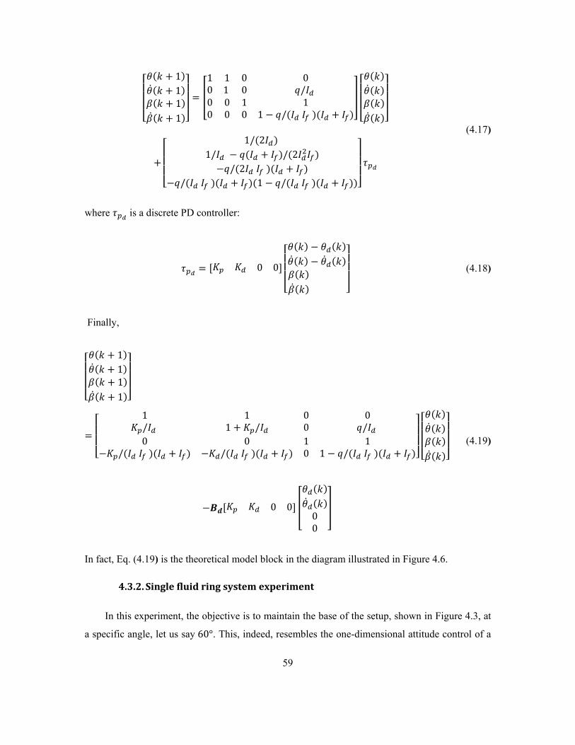
⎣⎢⎢⎢⎡𝜃

(𝑘 + 1)�̇�(𝑘 + 1)𝛽(𝑘 + 1)�̇�(𝑘 + 1)⎦

⎥⎥⎥⎤

= �

1 1 0 00 1 0 𝑞/𝐼𝑑 0 0 1 10 0 0 1 − 𝑞/(𝐼𝑑 𝐼𝑓 )(𝐼𝑑 + 𝐼𝑓)

�

⎣⎢⎢⎢⎡𝜃

(𝑘)�̇�(𝑘)𝛽(𝑘)�̇�(𝑘)⎦

⎥⎥⎥⎤

+

⎣⎢⎢⎢⎡

1/(2𝐼𝑑) 1/𝐼𝑑 − 𝑞(𝐼𝑑 + 𝐼𝑓)/(2𝐼𝑑2𝐼𝑓)−𝑞/(2𝐼𝑑 𝐼𝑓 )(𝐼𝑑 + 𝐼𝑓)

−𝑞/(𝐼𝑑 𝐼𝑓 )(𝐼𝑑 + 𝐼𝑓)(1 − 𝑞/(𝐼𝑑 𝐼𝑓 )(𝐼𝑑 + 𝐼𝑓))⎦⎥⎥⎥⎤𝜏𝑝𝑑

(4.17)

where 𝜏𝑝𝑑 is a discrete PD controller:

𝜏𝑝𝑑 = [𝐾𝑝 𝐾𝑑 0 0]

⎣⎢⎢⎢⎡𝜃

(𝑘) − 𝜃𝑑(𝑘)�̇�(𝑘) − �̇�𝑑(𝑘)𝛽(𝑘) �̇�(𝑘) ⎦

⎥⎥⎥⎤ (4.18)

Finally,

⎣⎢⎢⎢⎡𝜃

(𝑘 + 1)�̇�(𝑘 + 1)𝛽(𝑘 + 1)�̇�(𝑘 + 1)⎦

⎥⎥⎥⎤

=

⎣⎢⎢⎡

1 1 0 0𝐾𝑝/𝐼𝑑 1 + 𝐾𝑝/𝐼𝑑 0 𝑞/𝐼𝑑

0 0 1 1−𝐾𝑝/(𝐼𝑑 𝐼𝑓 )(𝐼𝑑 + 𝐼𝑓) −𝐾𝑑/(𝐼𝑑 𝐼𝑓 )(𝐼𝑑 + 𝐼𝑓) 0 1 − 𝑞/(𝐼𝑑 𝐼𝑓 )(𝐼𝑑 + 𝐼𝑓)⎦

⎥⎥⎤

⎣⎢⎢⎢⎡𝜃

(𝑘)�̇�(𝑘)𝛽(𝑘)�̇�(𝑘)⎦

⎥⎥⎥⎤

−𝑩𝒅[𝐾𝑝 𝐾𝑑 0 0] �

𝜃𝑑(𝑘)�̇�𝑑(𝑘)

00

�

(4.19)

In fact, Eq. (4.19) is the theoretical model block in the diagram illustrated in Figure 4.6.

4.3.2. Single fluid ring system experiment

In this experiment, the objective is to maintain the base of the setup, shown in Figure 4.3, at

a specific angle, let us say 60°. This, indeed, resembles the one-dimensional attitude control of a

59

satellite, which is achievable using only one fluid ring actuator. To this end, 𝜃𝑑 = 60° and

�̇�𝑑 = 0 rad/s are substituted into Eq. (4.19) to obtain the desired fluid angular velocity �̇�d, which

produces the necessary control torque. The desired impeller speed, that leads to �̇�d sought, is then

found from Eq. (4.2), which is modified as per the equation below:

�𝜔𝑖𝑚𝑝 = 7 𝑡 < 30 𝑠𝜔𝑖𝑚𝑝 = 1/0.11(�̇�d + 0.11) + 7 𝑡 ≥ 30 𝑠

� (4.20)

The reason for this modification lies in the fact that the setup does not operate properly for the

impeller speeds of less than 4 rad/s due to the friction and inertial effects. In Eq. (4.20), the value

of 7 rad/s is assigned to the first 30 seconds of the experiment so as to allow the operator to

initialize the attitude angle of the setup, let say at zero degree. The same offset is applied after

𝑡 = 30 s in Eq. (4.20) to compensate the internal friction of the system. The input voltage to the

pump is finally calculated using Eq. (4.8). Here, the angular velocity of the base is measured by a

gyroscope and transmitted to a computer using radio signals. Although a Kalman filter was used

to cancel out the noises existing in the signals, limitations in the computational speed of the

computer used did not allow for a real time filter. Therefore, the Kalman filter was only used

offline at the data processing stage. Here, a word of caution is in order: since the Kalman filter is

implemented offline, the measurement data already contain the effect of the observation noise and

its covariance matrix, ν(k + 1) and R(k + 1), introduced in the equations pertaining to the design

of the Kalman filter. With this regard, indeed, there is no need to consider Q(k + 1) that denotes

the covariance matrix of the process noise.

Figures 4.7−4.11 present the variation of various important quantities versus time obtained

from the theory and the experiment. From Figure 4.7, it can be concluded that the difference

between the impeller angular velocity obtained from the theory and the experiment is small; this

is slightly higher in the first 10 seconds but diminishes over time. The same effect can be

observed in the rotation angle and angular velocity plots of the disk shown in Figures 4.8 and 4.9,

respectively. The reason for this difference lies in the Coulomb friction forces existing inside the

pump and also the time delay in the communication of the control input. At t = 25 𝑠, a jump is

observed in the actual impeller angular velocity plot in Figure 4.7. This is due to either the

instantaneous malfunction of the impeller caused by air pockets or the loss of data sent by the

60

controller. This jump could not be avoided in any trials of the experiment, though the time of its

occurrence varied.

Figure 4.7: Theoretical and experimental plots of the impeller angular velocity versus time

Figure 4.8: Theoretical and experimental plots of the attitude angle of the disk versus time

Another observation in Figure 4.8 is that, in the experiment, the slope of the plot of the attitude

angle of the base versus time is less than what is expected from the theory. The reason behind is

that the impeller has an initial error in tracking the input control command. This error has also

affected the base angular velocity plotted in Figure 4.9; to correct this error, the PD controller has

produced a quite large control command at 𝑡 = 6 s. Despite the difference discussed in this

section, the results of the theory and the experiment have trends, which are reasonably close.

Figures 4.10 and 4.11 show the control torque produced and the input voltage required by

the pump, respectively. From the former, the maximum torque produced is about 0.007 N. m,

which is quite small. However, according to Figure 4.11, to produce this torque, the voltage

61

required is more than 10 V. This reveals the need for a high voltage to produce the required

control torque.

Figure 4.9: The theoretical and experimental plots of the disk angular velocity versus time

Figure 4.10: The experimental control torque versus time

Figure 4.11: Input voltage which is applied to the fluid ring system

62

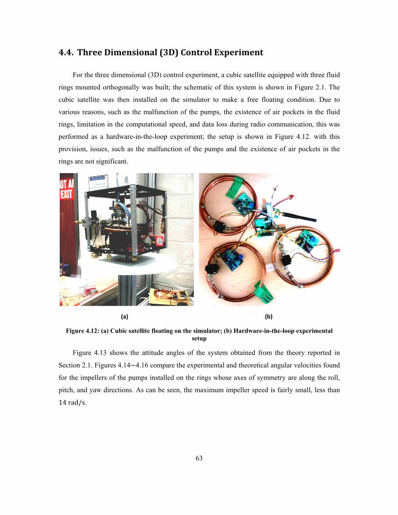
4.4. Three Dimensional (3D) Control Experiment

For the three dimensional (3D) control experiment, a cubic satellite equipped with three fluid

rings mounted orthogonally was built; the schematic of this system is shown in Figure 2.1. The

cubic satellite was then installed on the simulator to make a free floating condition. Due to

various reasons, such as the malfunction of the pumps, the existence of air pockets in the fluid

rings, limitation in the computational speed, and data loss during radio communication, this was

performed as a hardware-in-the-loop experiment; the setup is shown in Figure 4.12. with this

provision, issues, such as the malfunction of the pumps and the existence of air pockets in the

rings are not significant.

(a)

(b)

Figure 4.12: (a) Cubic satellite floating on the simulator; (b) Hardware-in-the-loop experimental setup

Figure 4.13 shows the attitude angles of the system obtained from the theory reported in

Section 2.1. Figures 4.14−4.16 compare the experimental and theoretical angular velocities found

for the impellers of the pumps installed on the rings whose axes of symmetry are along the roll,

pitch, and yaw directions. As can be seen, the maximum impeller speed is fairly small, less than

14 rad/s.

63

Figure 4.13: Attitude angles found from the theoretical model

Figure 4.14: Theoretical and Experimental angular velocities of the roll-axis impeller

Figure 4.15: Theoretical and Experimental angular velocities of the pitch-axis impeller

64

Figure 4.16: Theoretical and Experimental angular velocities of the yaw-axis impeller

Figure 4.17 shows the desired fluid angular velocity found upon substituting the desired

impeller angular velocities of Figures 4.14-4.16 into Eq. (4.20). As can be noticed, the maximum

angular velocity of the fluid, that is 1.4 rad/s, occurs in the first 20 seconds of the experiment.

As time progresses, the fluid angular velocity in different rings reduces to 0.5 rad/s, as expected

from the bias angular velocity existing in Eq. (4.20) .

Figure 4.18 shows the applied voltage to produce the fluid angular velocity, and hence, the

torque required. Accordingly, to produce the maximum fluid angular velocity of 1.4 rad/s, the

voltage required is about 13 V, which is quite high. Considering the light structure of the cubic

satellite used in this experiment, one can readily conclude that the application of fluid ring

actuators in typical satellites requires high input voltages of more than 12 V. This in turns reveals

the necessity of using massive batteries; more fuel is then required to launch the satellite to its

orbit. Therefore, the application of fluid rings as primary means of stabilizing the attitude of

satellites is not really a practical option. Nevertheless, fluid ring actuators bring interesting

advantages to either satellites requiring small-magnitude torque for attitude stabilization, or as

auxiliary attitude control actuators; the latter is discussed in detail in Chapters 5 and 6.

65

(a)

(b)

(c)

Figure 4.17: Desired fluid angular velocity in the: (a) Roll-axis ring; (b) Pitch-axis ring; (c) Yaw-axis ring

66

(a)

(b)

(c)

Figure 4.18: Applied voltage to the pumps on different rings versus time: (a) roll-axis; (b) pitch-axis; (c) yaw axis

67

4.5. Summary

In this chapter, a few experiments were conducted to validate the concept of utilizing fluid ring

actuators. To this end, first, the selection of the material for the fabrication of the ring, the type of

the pump, and the fluid were discussed. A copper ring which is equipped with a small centrifugal

pump was built. The ring was filled with ethylene glycol, which is an antifreeze liquid and has

appropriate characteristics for space applications. To perform the experiments, the empirical

relation between the input voltage of the pump and the fluid angular velocity was found. Next, an

experiment with a single fluid ring mounted on the simulator was conducted. The input voltage

was applied to this system using a PD controller. The results achieved from the single fluid ring

system were satisfactory, thus proving the concept of using fluid ring actuators. Next, a three

dimensional attitude stabilization experiment was presented. Due to various imperfections, such

as the malfunction of the pumps, the existence of air pockets in the fluid rings, and data loss

during radio communication, this was performed as a hardware-in-the-loop experiment. Despite

the pertinence of the results, it was concluded that, to produce a small fluid angular velocity of

1.5 rad/s, a quite high voltage of about 13 V is required. Indeed, this fact limits the applications

of the fluid rings as auxiliary actuators.

68

Chapter 5

SPINNING SATELLITES WITH FLUID RING

ACTUATORS

The results of the experiments, reported in Chapter 4, showed that the fluid rings require a

quite high voltage (above 12 V) to produce a fluid angular velocity that is greater than 2 rad/s.

To produce this voltage, large-size batteries are required, which increase the overall mass of the

satellite, and thus the total cost of the mission. Despite this drawback, the low mass of the fluid

rings and their easy implementation justify the search for other applications, such as auxiliary

attitude stabilization actuators. In this chapter, the use of fluid rings in spinning satellites is

studied. A spinning satellite resists any variation of its orientation because of the bias momentum

resulting from spinning about one of its axes. However, natural disturbances, such as solar

radiation pressure, adversely affect the orientation of spinning satellites. The error resulting from

such disturbance can be eliminated using a relatively small control torque. The application of

fluid rings to pursue this objective is discussed in this chapter.

69

5.1. Development of the Dynamical Model

The system considered here is a symmetric spinning satellite consisting of two fluid rings

whose axes of symmetry are aligned with the roll and yaw axes, as depicted in Figure 5.1.

Figure 5.1: A cylindrical satellite with two fluid rings

The center of mass of each of the two fluid rings is assumed to coincide with that of the

satellite. A local vertical and local horizontal (LVLH) reference frame with its origin located at

the center of mass of the satellite is defined as follows: 𝑋0 is along the local horizontal; 𝑌0 is

perpendicular to the orbital plane; and 𝑍0 is directed towards the center of the Earth (Wie, 1998).

The LVLH frame rotates about the Earth at the orbital rate of 𝑛. A spinning frame is defined that

initially coincides with the LVLH reference frame; this frame spins about the 𝑌0-axis with respect

to the LVLH frame with the angular velocity Ω. The third reference frame defined is the body

fixed frame of the satellite whose axes coincide with the principal axes of the satellite; this frame

is identical to the spinning frame, if the satellite does not tilt. Figure 5.2 shows the three

coordinate frames introduced; for better visualization, the origin of the frames are shown non-

coincident. The orientation of the satellite at any instant is described by three rotation angles, 𝜃1,

𝜃2, and 𝜃3, respectively, about the 𝑋, 𝑌, and Z axes of the body fixed frame with respect to the

LVLH frame. Also, Θ1, Θ2 , and Θ3 denote another set of rotation angles which describes the

rotation of the body fixed frame with respect to the spinning frame. The relations between the

attitude angles, 𝜃1, 𝜃2, and 𝜃3, and the set of rotation angles Θ1, Θ2, and Θ3 are

𝜃1 = Θ1, 𝜃2=Θ2 + Ω𝑡, 𝜃3 = Θ3 (5.1)

Z

X

Y

Fluid ring

70

Figure 5.2: Three coordinates frames used in dynamical modeling

Figure 5.3: Free body diagrams of the satellite and two fluid rings (only moment vectors are shown)

The equations of motion of a spinning satellite with two fluid rings are derived using Eqs.

(2.2) and (2.10) from Chapter 2. To this end, the term ∑ 𝑹𝒊𝝉𝒓𝒊2𝑖=1 is expanded, the rotation

matrices 𝑹𝟏 and 𝑹𝟐 being recalled from Eq. (2.3).

𝑰𝒔�̇� + 𝝎 × 𝑰𝒔𝝎 = 𝝉𝒈𝒈 + 𝝉𝒓𝟏 + 𝝉𝒓𝟑 (5.2)

𝑰𝒇𝟏��̇� + 𝜷�̈� + 𝝎 × �̇�𝟏� + 𝝎 × 𝑰𝒇𝟏�𝝎 + �̇�𝟏� = −𝝉𝒓𝟏 + 𝝉𝒈𝒈𝒇𝟏 (5.3)

𝑰𝒇𝟑��̇� + 𝜷�̈� + 𝝎 × �̇�𝟑� + 𝝎 × 𝑰𝒇𝟑�𝝎 + �̇�𝟑� = −𝝉𝒓𝟑 + 𝝉𝒈𝒈𝒇𝟑 (5.4)

Z

X

Y

𝒎𝟏𝟑

𝒎𝟐𝟑 𝒎𝟐𝟏

𝒎𝟑𝟏

𝝉𝒇𝟏

𝝉𝒇𝟑

𝝉𝒇𝟏, 𝒎𝟏𝟑

𝝉𝒇𝟑,𝒎𝟑𝟏

𝒎𝟐𝟏,𝒎𝟐𝟑 𝝉𝒈𝒈 𝝉𝒈𝒈𝒇𝟑 𝝉𝒈𝒈𝒇𝟏

𝑍0

z

Z

𝑋0

𝑥

X

𝑦

Y

𝑂 𝑂

𝑂

Ω + n

𝑛

LVLH

Spinning frame

Body-fixed frame

Ω + n

𝑌0

71

where 𝝉𝒓𝟏 = [𝜏𝑓1 𝑚21 𝑚31]𝑇 and 𝝉𝒓𝟑 = [𝑚13 𝑚23 𝜏𝑓3]𝑇 . Equations (5.2)-(5.4) are

written in the body fixed frame of the satellite. The inertia matrix of the satellite, without

considering the fluid itself, is denoted by 𝑰𝒔. Let us assume here that 𝑰𝒔 is diagonal with non-zero

entries of 𝐼𝑡, 𝐼𝑎 , 𝐼𝑡 in the roll, pitch, and yaw directions, respectively; the 𝑦-axis is the axis of

symmetry of the cylindrical satellite as per Figure 5.1. The axes of symmetry of the fluid rings are

aligned with the roll and yaw axes; the inertia matrices of the fluid rings are as expressed below:

𝑰𝒇𝟏 = �𝐼𝑓 0 00 𝐼𝑓/2 00 0 𝐼𝑓/2

�, 𝑰𝒇𝟑 = �𝐼𝑓/2 0 0

0 𝐼𝑓/2 00 0 𝐼𝑓

�, 𝐼𝑓 = 2𝜋𝜌𝐴𝑟3 (5.5)

where 𝜌, 𝐴, and 𝑟 denote the fluid density, the fluid ring cross-sectional area, and the fluid ring

radius, respectively. Further, 𝝉𝒈𝒈, 𝝉𝒈𝒈𝒇𝟏 , and 𝝉𝒈𝒈𝒇𝟑 are gravity gradient torques exerted on the

satellite and the fluid rings. The terms �̇�𝟏 = [�̇�1 0 0]𝑇 and �̇�𝟑 = [0 0 �̇�3]𝑇 are the angular

velocity vectors of the fluid relative to the fluid loops. The free body diagrams of the satellite and

each fluid rings are depicted in Figure 5.3. In this figure, 𝑚𝑖𝑗 for 𝑖 = 1, 2 and 𝑗 = 1, 3 is the

reaction moment in the 𝑖th direction exerted by the 𝑗th fluid ring on the satellite. The reaction

moments 𝑚𝑖𝑗 can be found from Eqs. (5.3) and (5.4) as:

𝑚21 = −𝒆𝟐𝑇[𝑰𝒇𝟏��̇� + 𝜷�̈� + 𝝎 × �̇�𝟏� + 𝝎 × 𝑰𝒇𝟏�𝝎 + �̇�𝟏� − 𝝉𝒈𝒈𝒇𝟏] (5.6)

𝑚31 = −𝒆𝟑𝑇[𝑰𝒇𝟏��̇� + 𝜷�̈� + 𝝎 × �̇�𝟏� + 𝝎 × 𝑰𝒇𝟏�𝝎 + �̇�𝟏� − 𝝉𝒈𝒈𝒇𝟏] (5.7)

𝑚13 = −𝒆𝟏𝑇[𝑰𝒇𝟑��̇� + 𝜷�̈� + 𝝎 × �̇�𝟑� + 𝝎 × 𝑰𝒇𝟑�𝝎 + �̇�𝟑� − 𝝉𝒈𝒈𝒇𝟑] (5.8)

𝑚23 = −𝒆𝟐𝑇[𝑰𝒇𝟑��̇� + 𝜷�̈� + 𝝎 × �̇�𝟑� + 𝝎 × 𝑰𝒇𝟑�𝝎 + �̇�𝟑� − 𝝉𝒈𝒈𝒇𝟑] (5.9)

where 𝒆𝟏 = [1 0 0]𝑇 , 𝒆𝟐 = [0 1 0]𝑇 , and 𝒆𝟑 = [0 0 1]𝑇 . Since 𝒆𝒊𝑻�̈�𝒋 vanishes

identically, Eqs. (5.6)−(5.9) can be used to replace 𝑚𝑖𝑗 in Eq. (5.2). Hence, the equations of

motion of the satellite are obtained free of the fluid angular acceleration terms which can then be

solved using a stable numerical integrator. In fact, the fluid acceleration terms only appear in the

equations below, which are the first row of Eq. (5.3) and the third row of Eq. (5.4).

72

𝐼𝑓�̈�1 + 𝒆𝟏𝑇 �𝑰𝒇𝟏��̇� + 𝝎 × �̇�𝟏� + 𝝎 × 𝑰𝒇𝟏�𝝎 + �̇�𝟏� − 𝝉𝒈𝒈𝒇𝟏� + 𝜏𝑓1 = 0 (5.10)

𝐼𝑓�̈�𝑖 + 𝒆𝟑𝑇 �𝑰𝒇𝟑��̇� + 𝝎 × �̇�𝟑� + 𝝎 × 𝑰𝒇𝟑�𝝎 + �̇�𝟑� − 𝝉𝒈𝒈𝒇𝟑� + 𝜏𝑓3 = 0 (5.11)

The solution of Eqs. (5.10) and (5.11) yields the angular acceleration of the fluid.

5.2. Small Angle Approximation

Designing a controller for the system with the nonlinear mathematical model expressed in

Eqs. (5.2), (5.10), and (5.11) is not straightforward. Therefore, to obtain some insight into the

system dynamics, it is necessary to first approach the problem with a simplifying assumption on

the magnitude of the attitude angles: the angles in question are small enough to allow

simplification expressed hereafter. Before adopting the assumption on the magnitude of the

angles in the mathematical model of the system, it is required to express these equations in terms

of Θ1, Θ2, and Θ3. In fact, the attitude angle 𝜃2, which is the rotation angle of the satellite about

the spin axis, continuously grows, thus cannot be assumed small. However, the small angle

assumption can be applied to 𝜃1 and 𝜃3 . As mentioned earlier, the nominal spin rate of the

satellite is denoted by Ω. Therefore, the absolute angular rate of the spinning frame is 𝜈 = Ω +

𝑛, as the satellite is considered to be in a circular orbit. The equations below relate the satellite

angular velocity to the angles Θ1 , Θ2 , and Θ3 and their derivatives using the small angle

approximation (Hughes, 1986).

𝜔1 = Θ̇1 − 𝜈Θ3 → �̇�1 = Θ̈1 − 𝜈Θ̇3

𝜔2 = Θ̇2 − 𝜈 → �̇�2 = Θ̈2

𝜔3 = Θ̇3 + 𝜈Θ1 → �̇�3 = Θ̈3 + 𝜈Θ̇1

(5.12)

The gravity gradient torque exerted on the satellite can be obtained as (Schaub and Junkins,

2003):

𝝉𝒈𝒈 = −3𝑛2𝒂�𝟑 × 𝑱.𝒂�𝟑 (5.13)

73

where 𝒂�𝟑 ≡ 𝒓𝒄/‖𝒓𝒄‖, 𝒓𝒄 being the position vector of the center of mass of the satellite with

respect to the Earth center, described in the LVLH frame. To evaluate 𝝉𝒈𝒈 in the body fixed

frame of the satellite, 𝒂�𝟑 is required to be expressed in this frame; this is possible upon applying

the rotation matrix 𝑪 defined below:

𝑪 = 𝑪𝟏(Θ1)𝑪𝟐(Θ2)𝑪𝟑(Θ3)𝑪𝟐(−Ωt) (5.14)

where 𝑪𝒊�Θ𝑗� is the matrix associated with the rotation of the angle Θ𝑗 about the 𝑖th axis. Using

Eq. (5.14), under the assumption of infinitesimal attitude angles, the gravity gradient torque can

be obtained in the satellite body-fixed frame as:

𝝉𝒈𝒈 = −3𝑛2 ��𝐼𝑦𝑦 − 𝐼𝑧𝑧�(Θ3 sinΩ𝑡 cosΩ𝑡 + Θ1 cos2 Ω𝑡)

(𝐼𝑧𝑧 − 𝐼𝑥𝑥)(Θ2 sin2 Ω𝑡 − Θ2sinΩ𝑡 cosΩ𝑡 − Θ2 cos2 Ω𝑡)�𝐼𝑥𝑥 − 𝐼𝑦𝑦�(−Θ3 sin2 Ω𝑡 − Θ1 cosΩ𝑡 sinΩ𝑡)

� (5.15)

In order to obtain the equation of motion of the satellite, Eqs. (5.2)−(5.4) are rewritten

considering Eqs. (5.12) and (5.15). As mentioned before, the diagonal moment of inertia matrix

of the satellite is 𝑰𝒔= diag(𝐼𝑥𝑥 = 𝐼𝑡 , 𝐼𝑦𝑦 = 𝐼𝑎 , 𝐼𝑧𝑧 = 𝐼𝑡); therefore, the gravity gradient torque is

zero in the 𝑌 direction. The equation describing the satellite rotation about the 𝑌 axis is not

included, as it has the simple form: 𝐼𝑎Θ̈2 = 0. Moreover, as stated in Eq. (5.1), Θ1 = 𝜃1 and

Θ3 = 𝜃3; thus, we have

�𝐼𝑡 + 𝐼𝑓/2��̈�1 − �2𝐼𝑡 − 𝐼𝑎 + 𝐼𝑓�𝜈�̇�3

+�𝐼𝑎 − 𝐼𝑡 − 𝐼𝑓/2�[𝜈2𝜃1 + 3𝑛2(𝜃1𝑐 + 𝜃3𝑠)𝑐] − 𝜏𝑓1 − 𝐼𝑓𝜈�̇�3 = 0 (5.16)

�𝐼𝑡 + 𝐼𝑓/2��̈�3 + �2𝐼𝑡 − 𝐼𝑎 + 𝐼𝑓�𝜈�̇�1

+�𝐼𝑎 − 𝐼𝑡 − 𝐼𝑓/2�[𝜈2𝜃3 + 3𝑛2(𝜃1𝑐 + 𝜃3𝑠)𝑠] − 𝜏𝑓3 + 𝐼𝑓𝜈�̇�1 = 0 (5.17)

𝐼𝑓(�̈�1 + �̈�1) + 𝜏𝑓1 − 𝐼𝑓𝜈�̇�3 = 0 (5.18)

𝐼𝑓(�̈�3 + �̈�3) + 𝜏𝑓3 + 𝐼𝑓𝜈�̇�1 = 0 (5.19)

74

Here, 𝑠 and 𝑐 denote sinΩ𝑡 and cosΩ𝑡, respectively. Next, a new set of variables 𝛾1and 𝛾3 are

defined in order to eliminate the periodic coefficients of 𝑠 and 𝑐 from Eqs. (5.16) and (5.17)

(Hughes, 1986):

�𝜃1𝜃3� = �cosΩ 𝑡 sinΩt

−sinΩt cosΩt� �𝛾1𝛾3�

(5.20)

Upon introducing this new set of variables, the abovementioned equations of motion of the

spinning satellite become

�𝐼𝑡 + 𝐼𝑓/2�(�̈�1𝑐 − �̈�3𝑠) + �2𝐼𝑡𝑛 + 𝐼𝑎𝜈 + 𝐼𝑓𝑛�(�̇�1𝑠 + �̇�3𝑐)

−[𝐼𝑎(𝑛𝜈 − 3𝑛2) + 4𝐼𝑡𝑛2 + 2𝐼𝑓𝑛2]𝛾1𝑐 + �𝐼𝑎𝑛𝜈 + 𝐼𝑡𝑛2 + 𝐼𝑓/2𝑛2�𝛾3𝑠

−𝜏𝑓1 − 𝐼𝑅𝜈�̇�3 = 0

(5.21)

�𝐼𝑡 + 𝐼𝑓/2�(�̈�1𝑠 + �̈�3𝑐) − �2𝐼𝑡𝑛 + 𝐼𝑎𝜈 + 𝐼𝑓𝑛�(�̇�1𝑐 − �̇�3𝑠)

−[𝐼𝑎(𝑛𝜈 − 3𝑛2) + 4𝐼𝑡𝑛2 + 2𝐼𝑓𝑛2]𝛾1𝑠 − �𝐼𝑎𝑛𝜈 + 𝐼𝑡𝑛2 + 𝐼𝑓/2𝑛2�𝛾3𝑐

−𝜏𝑓3 + 𝐼𝑓𝜈�̇�1 = 0

(5.22)

𝐼𝑓(�̈�1 + �̈�1𝑐 − �̈�3𝑠) + �2𝐼𝑓𝑛 + 𝐼𝑓𝜈��̇�1𝑠 + �2𝐼𝑓𝑛 + 𝐼𝑓𝜈��̇�3𝑐

−�𝐼𝑓𝑛𝜈 + 𝐼𝑓𝑛2�𝛾1𝑐 + �𝐼𝑓𝑛𝜈 + 𝐼𝑓𝑛2�𝛾3𝑠 + 𝜏𝑓1 = 0 (5.23)

𝐼𝑓(�̈�3 + �̈�1𝑠 + �̈�3𝑐) − �2𝐼𝑓𝑛 + 𝐼𝑓𝜈��̇�1𝑐 + �2𝐼𝑓𝑛 + 𝐼𝑓𝜈��̇�3𝑠

−�𝐼𝑓𝑛𝜈 + 𝐼𝑓𝑛2�𝛾1𝑠 − �𝐼𝑓𝑛𝜈 + 𝐼𝑓𝑛2�𝛾3𝑐 + 𝜏𝑓3 = 0 (5.24)

In order to proceed to design a linear controller for the system, first, we need to eliminate the

time-varying variables denoted by 𝑠 and 𝑐 from Eqs. (5.21) and (5.22). This is done in two steps:

(i) The time-varying coefficient of the terms �̈�1 and �̈�3 are first eliminated by obtaining two new

equations via forming the linear combination of the two equations in question, as per the relation

below:

𝐸𝑞. (5.21) 𝑐 + 𝐸𝑞. (5.22) 𝑠 =0

−𝐸𝑞. (5.21) 𝑠 + 𝐸𝑞. (5.22) 𝑐 =0 (5.25)

75

Expanding Eq. (5.25) yields:

�𝐼𝑡 + 𝐼𝑓/2��̈�1 + �2𝐼𝑡𝑛 + 𝐼𝑎𝜈 + 𝐼𝑓𝑛��̇�3 − [𝐼𝑎(𝑛𝜈 − 3𝑛2) + 4𝐼𝑡𝑛2 + 2𝐼𝑓𝑛2]𝛾1

−𝜏𝑓1𝑐 − 𝐼𝑓𝜈�̇�3𝑐 − 𝜏𝑓3𝑠 + 𝐼𝑓𝜈�̇�1𝑠 = 0 (5.26)

�𝐼𝑡 + 𝐼𝑓/2��̈�3 − �2𝐼𝑡𝑛 + 𝐼𝑎𝜈 + 𝐼𝑓𝑛��̇�1 − [𝐼𝑎𝑛𝜈 + 𝐼𝑡𝑛2 + 𝐼𝑓/(2𝑛^2 )]𝛾3

+𝜏𝑓1𝑠 + 𝐼𝑓𝜈�̇�3𝑠 − 𝜏𝑓3𝑐 + 𝐼𝑓𝜈�̇�1𝑐 = 0 (5.27)

(ii) The remaining terms with the time-varying coefficient 𝑠 and 𝑐 are handled by regrouping the

variables. A control input can be defined that includes the terms having the time-varying

coefficient. This control input simplifies the controller design. However, prior to this operation,

the variables are non-dimensionalized.

5.2.1. Non-dimensionalization

In order to reduce the effect of computational errors and enhance the applicability of the

results, equations obtained in the preceding section are non-dimensionalized. To this end, the

non-dimensional time variable 𝑇 = 𝑛𝑡 is used, similar to Subsection 2.1.1. The non-dimensional

angular velocity terms can then be defined as:

𝛾1′ ≡ �̇�1/𝑛, 𝛾3′ ≡ �̇�3/𝑛, 𝛽1′ ≡ �̇�1/𝑛, 𝛽3′ ≡ �̇�3/𝑛, �̂� ≡ (Ω/n) + 1 (5.28)

Hence, the non-dimensional form of Eqs. (5.23), (5.24), (5.26), and (5.27) are:

(𝐾𝑡 + 𝐾𝑅/2)𝛾1′′ + (2𝐾𝑡 + �̂� + 𝐾𝑅)𝛾3′ − [(�̂� − 3) + 4𝐾𝑡 + 2𝐾𝑅]𝛾1

−�̂�𝑓1𝑐 − 𝐾𝑅𝜈�𝛽3′ 𝑐 − 𝜏�𝑓3𝑠 + 𝐾𝑅𝜈�𝛽1

′ 𝑠 = 0 (5.29)

(𝐾𝑡 + 𝐾𝑅/2)𝛾1′′ + (2𝐾𝑡 + �̂� + 𝐾𝑅)𝛾3′ − [(�̂� − 3) + 4𝐾𝑡 + 2𝐾𝑅]𝛾1

−�̂�𝑓1𝑐 − 𝐾𝑅𝜈�𝛽3′ 𝑐 − 𝜏�𝑓3𝑠 + 𝐾𝑅𝜈�𝛽1

′ 𝑠 = 0 (5.30)

𝐾𝑅[𝛽1′′ + 𝛾1′′𝑐 − 𝛾3′′𝑠 + (2 + �̂�)(𝛾1′𝑠 + 𝛾3′𝑐) − (1 + �̂�)(𝛾1𝑐 − 𝛾3𝑠)] + �̂�𝑓1 = 0 (5.31)

𝐾𝑅[𝛽3′′ + 𝛾1′′𝑠 + 𝛾3′′𝑐 − (2 + �̂�)(𝛾1′𝑐 − 𝛾3′𝑠) − (1 + �̂�)(𝛾1𝑠 + 𝛾3𝑐)] + �̂�𝑓3 = 0 (5.32)

76

where 𝐾𝑡, 𝐾𝑅 are the inertia ratios defined below:

𝐾𝑡 ≡ 𝐼𝑡/𝐼𝑎 , 𝐾𝑅 ≡ 𝐼𝑓/𝐼𝑎 (5.33)

Moreover, �̂�𝑓1 and �̂�𝑓3 are non-dimensional form of the fluid friction torques, as defined earlier in

Eq. (2.26):

�̂�𝑓𝑖 = −16 𝜋 𝑎1𝑎2�̂�𝛽𝑖′, for 𝑖 = 1, 3 (5.34)

where �̂�, 𝑎1, and 𝑎2 are the non-dimensional parameters defined below:

�̂� ≡ 𝑑/𝑟 , 𝑎1 ≡ (𝜌𝜋𝑟5)/𝐼𝑎 , 𝑎2 ≡ 𝜇/(𝜌𝑟𝑛𝐷) (5.35)

5.3. Design of a Controller for the Linear Model

To design a controller, the control input terms 𝜏1𝑐 and 𝜏3𝑐 are added to the right hand side of

the equations of motion of the satellite (5.29) and (5.30). As discussed in Section 5.2, a

regrouping of the variables is needed to eliminate the time-varying coefficients 𝑠 and 𝑐 from Eqs.

(5.29) and (5.30); this leads to

(𝐾𝑡 + 𝐾𝑅/2)𝛾1′′ + (2𝐾𝑡 + �̂� + 𝐾𝑅)𝛾3′ − [(�̂� − 3) + 4𝐾𝑡 + 2𝐾𝑅]𝛾1 = 𝑣1𝑐 (5.36)

(𝐾𝑡 + 𝐾𝑅/2)𝛾3′′ − (2𝐾𝑡 + �̂� + 𝐾𝑅𝑛)𝛾1′ − (�̂� + 𝐾𝑡 + 𝐾𝑅/2)𝛾3 = 𝑣3𝑐 (5.37)

where

𝑣1𝑐 = 𝜏1𝑐 − (−�̂�𝑓1𝑐 − 𝐾𝑅�̂�𝛽3′𝑐 − �̂�𝑓3𝑠 + 𝐾𝑅�̂�𝛽1′𝑠) (5.38)

𝑣3𝑐 = 𝜏3𝑐 − (�̂�𝑓1𝑠 + 𝐾𝑅�̂�𝛽3′𝑠 − �̂�𝑓3𝑐 + 𝐾𝑅�̂�𝛽1′𝑐) (5.39)

Since Eqs. (5.36) and (5.37) are linear, a controller can be designed using the pole placement

method, which is simple to implement. To this end, the system equations are first expressed in the

state-space form:

�̇� = 𝑨𝒙 + 𝑩𝒗 (5.40)

77

where 𝒙 = [𝑥1 𝑥2 𝑥3 𝑥4]𝑇 is the state vector of the system with 𝑥1 = 𝛾1, 𝑥2 = 𝛾1′ , 𝑥3 = 𝛾3,

and 𝑥4 = 𝛾3′ . The matrices 𝑨 and 𝑩 are

𝑨 = �

0 1 0 0𝑞1 0 0 −𝑞20 0 0 10 𝑞3 𝑞4 0

� , 𝑩 = �

0 01 00 00 1

� (5.41)

where

𝑞1 = [(�̂� − 3) + 4𝐾𝑡 + 2𝐾𝑅]/(𝐾𝑡 + 𝐾𝑅/2); 𝑞2 = 𝑞3 = (2𝐾𝑡 + �̂� + 𝐾𝑅)/(𝐾𝑡 + 𝐾𝑅/2)

𝑞4 = (�̂� + 𝐾𝑡 + 𝐾𝑅/2)/(𝐾𝑡 + 𝐾𝑅/2) (5.42)

The controllability of the system can be determined by finding the rank of the controllability

matrix 𝑴 = [𝑩 𝑨𝑩 𝑨2𝑩 𝑨3𝑩] (Ogata, 2009). This matrix is full row rank, as in general,

𝑞1 𝑞4 is non-zero. The feedback control law applied to the system has the form 𝒗 = 𝑲𝒙, where

𝑲 = [𝛼4 − 𝑎4 𝛼3 − 𝑎3 𝛼2 − 𝑎2 𝛼1 − 𝑎1]𝑻−1 (5.43)

in which 𝑎𝑖 , for 𝑖 = 1, … ,4 are the coefficients of the characteristic equation of the open-loop

system:

𝑎1 = 0, 𝑎2 = 𝑞2 𝑞3 − 𝑞1 − 𝑞4, 𝑎3 = 0, 𝑎4 = 𝑞1 𝑞4 (5.44)

Further, parameters 𝛼𝑖 for 𝑖 = 1, … ,4 are the coefficients of the characteristic equation of the

closed loop system. To find these, for each control input 𝑣1𝑐 and 𝑣3𝑐, an appropriate set of poles 𝑝1

to 𝑝4 is chosen; here, for the sake of simplicity, identical values are chosen for different poles. In

Eq. (5.43), matrix 𝑻 = 𝑴𝑾, while 𝑾 is

𝑾 = �

𝑎3 𝑎2 𝑎1 1𝑎2 𝑎1 1 0𝑎1 1 0 01 0 0 0

� (5.45)

What has been obtained so far are the artificial control inputs 𝑣1𝑐 and 𝑣3𝑐. However, the objective

is to find the angular velocity magnitudes of the fluid in the two rings which stabilize the system.

To this end, upon adding the control inputs 𝜏1𝑐 and 𝜏3𝑐, the ordinary differential equations (5.31)

78

and (5.32) should be solved simultaneously with the algebraic equations (5.38) and (5.39). The

pertaining differential equations are repeated below for convenience. The solution process is that,

at every step, the values of 𝜏1𝑐 and 𝜏3𝑐 are obtained from Eqs. (5.38) and (5.39) knowing 𝛽1′ and 𝛽3′

at the same step. Substituting 𝜏1𝑐 and 𝜏3𝑐 into Eqs. (5.31) and (5.32), the equations below are

found from which the values of 𝛽1′ and 𝛽3′ can be obtained for the next step. The same process is

repeated to complete the solution.

𝐾𝑅[𝛽1′′ + 𝛾1′′𝑐 − 𝛾3′′𝑠 + (2 + �̂�)(𝛾1′𝑠 + 𝛾3′𝑐) − (1 + �̂�)(𝛾1𝑐 − 𝛾3𝑠)] + �̂�𝑓1 = −𝜏1𝑐 (5.46)

𝐾𝑅[𝛽3′′ + 𝛾1′′𝑠 + 𝛾3′′𝑐 − (2 + �̂�)(𝛾1′𝑐 − 𝛾3′𝑠) − (1 + �̂�)(𝛾1𝑠 + 𝛾3𝑐)] + �̂�𝑓3 = −𝜏3𝑐 (5.47)

5.3.1. Numerical results for the linear model

The performance of the controller and the fluid rings is examined by considering a 50 kg

cylindrical satellite with the radius and height of 0.3 m and 1 m , respectively. The principal

moments of inertia of the satellite about its center of mass are 𝐼𝑥𝑥 = 5.29 kgm2 , 𝐼𝑦𝑦 =

2.25 kgm2, and 𝐼𝑧𝑧 = 5.29 kgm2. Moreover, the same fluid rings and orbit are chosen as the case

study introduced in Chapters 2 and 3. This implies that the two fluid rings in the roll and yaw

directions are assumed to have a radius of 0.2 m and the cross-sectional diameter of 0.02 m, the

satellite is in an orbit with an altitude of 700 km. The initial values of the attitude angles, their

rates, and the relative angular velocity of the fluid in the fluid rings are chosen as π/36 rad,

10−4 rad/s, and zero, respectively. The spin rate of the satellite is considered to be 50𝑛, where

𝑛 = 1.1 × 10−3 rad/s is the mean orbital rate.

For the sake of simplicity, all poles desired are assumed to coincide. In general, large negative

poles result in a faster stabilization, but with more energy consumption. This implies that there is

a trade off in choosing the poles. In our problem, there is an additional significant constraint in

choosing the poles: they should not be too large not to violate the small-angle assumption. To

comply with this constraint, the attitude angles are considered to be bounded below 0.25 rad, the

poles being chosen as −10. Simulating the motion of the system, Figure 5.4 shows that the

satellite is stabilized in both the roll and yaw directions in about 0.2 of an orbital period.

79

Figure 5.4: Roll and yaw angles using the linear controller with 𝑝𝑖 = −10

Figure 5.5: Control torque in the roll and yaw directions using the linear controller with 𝑝𝑖 = −10

Figure 5.6: Fluid angular velocity using the linear controller with 𝑝𝑖 = −10

80

The control torque required to stabilize the satellite is plotted in Figure 5.5. The maximum

control torque required is less than 5 × 10−4 N. m, which is quite small. The variations of the

fluid angular velocity producing this control torque are also illustrated in Figure 5.6, the

maximum fluid angular velocity being about 1.5 × 10−3 rad/s.

5.4. Design of the Controller for the Nonlinear Model

In the light of the results obtained in the study of the linear model, in this section, a controller

is designed for the complete nonlinear model. To this end, the same approach is taken: we resort

to a modified control input vector 𝒗𝒄 = [𝜈1𝑐 0 𝜈3𝑐]𝑇, which includes all the terms with 𝑠 and 𝑐

coefficients; the equations of motion of the satellite (5.2) can thus be written as:

𝑰𝒔�̇� + 𝝎 × 𝑰𝒔𝝎 = 𝒗𝒄 (5.48)

𝑣𝑖𝑐 = 𝒆𝒊𝑻(𝝉𝒈𝒈 + [𝜏𝑓1 𝑚21 𝑚31]𝑇 + [𝑚13 𝑚23 𝜏𝑓3]𝑇) + �̃�𝑖𝑐 for 𝑖 = 1, 3 (5.49)

were 𝝉𝒄 = [�̃�1𝑐 0 �̃�3𝑐] , 𝒆𝟏 and 𝒆𝟑 being the unit vectors [1 0 0]𝑇 and [0 0 1]𝑇 ,

respectively. The fluid angular velocity in the two rings can be obtained from Eqs. (5.3) and (5.4)

reproduced below with the control input �̃�𝑖𝑐 for 𝑖 = 1, 3 implemented.

�̈�𝑖 = −𝒆𝒊 𝑻{�̇� + 𝝎 × �̇�𝒊 + 𝑰𝒇𝒊−𝟏[𝝎 × 𝑰𝒇𝒊�𝝎 + �̇�𝒊�] + 𝝉𝒈𝒈𝒇𝒊} + 𝜏𝑓𝑖 − �̃�𝑖𝑐 , for i = 1, 3 (5.50)

Before designing a controller, Eqs. (5.48)−(5.50) are non-dimensionalized as:

𝑰�𝒔𝝎′ + 𝝎� × 𝑰�𝒔𝝎� = 𝒗�𝒄 (5.51)

𝑣�𝑖𝑐 = 𝒆𝒊𝑻(𝝉�𝒈𝒈 + [�̂�𝑓1 𝑚�21 𝑚�31]𝑇 + [𝑚�13 𝑚�23 �̂�𝑓3]𝑇) + �̂�𝑖𝑐 (5.52)

𝛽𝑖′′ = 𝒆𝒊𝑻{𝝎′ + 𝝎� × 𝜷𝒊′ + 𝑰�𝒇𝒊−𝟏[𝝎� × 𝑰�𝒇𝒊(𝝎� + 𝜷𝒊′)] + 𝝉�𝒈𝒈𝒇𝒊} + �̂�𝑓𝑖 − �̂�𝑖𝑐 (5.53)

for 𝑖 = 1 and 3. Further, 𝑰�𝒔, 𝑰�𝒇𝟏, and 𝑰�𝒇𝟑 are the non-dimensional inertia matrices as follows:

81

𝑰�𝒔 = �𝐾𝑡 0 00 1 00 0 𝐾𝑡

� , 𝑰�𝒇𝟏 = �𝐾𝑅 0 00 𝐾𝑅/2 00 0 𝐾𝑅/2

� , 𝑰�𝒇𝟑 = �𝐾𝑅/2 0 0

0 𝐾𝑅/2 00 0 𝐾𝑅

� (5.54)

where 𝐾𝑡 and 𝐾𝑅 are given in Eq. (5.33). In the non-dimensional equations, 𝝎� , 𝝉�𝒈𝒈, 𝝉�𝒈𝒈𝒇𝒊are

𝝎� ≡ 𝝎/𝑛, 𝝉�𝒈𝒈 ≡ 𝝉𝒈𝒈/(𝑰𝒂 𝑛), 𝝉�𝒈𝒈𝒇𝒊 ≡ 𝝉𝒈𝒈𝒇𝒊/(𝑰𝒂𝑛) (5.55)

Now, a modified PD controller is designed as:

𝑣�𝑖𝑐 = 𝐾𝑝1𝑖(𝜃1 − 𝜃1𝑑) + 𝐾𝑑1𝑖(𝜃1′ − 𝜃1𝑑′ ) + 𝐾𝑝2𝑖(𝜃2 − 𝜃2𝑑) + 𝐾𝑑2𝑖(𝜃2

′ − 𝜃2𝑑′ ), for 𝑖 = 1,3 (5.56)

where the gains 𝐾𝑝1𝑖 , 𝐾𝑝2𝑖 , 𝐾𝑑1𝑖 , and 𝐾𝑑2𝑖 of the controller can be chosen from the feedback

control matrix 𝑲 obtained using the pole placement method in the linear analysis. This implies

that the elements of the first and second row of the matrix 𝑲 are to be used for the gains of the 𝑣�1𝑐

and 𝑣�2𝑐, respectively.

5.4.1. Numerical results for the nonlinear system

The performance of the fluid ring actuators in spinning satellites are discussed here when the

nonlinear dynamical model is used. The numerical parameters chosen are identical to the ones

introduced in Subsection 5.3.1. The gains of the modified PD control law are chosen from the

feedback controller obtained using the poles chosen as −10. In Figures 5.7 and 5.8, the pitch, roll

and yaw angles are plotted versus the number of orbits. The pitch angle linearly increases with

time due to the constant spin rate of the satellite. However, the roll and yaw angles are stabilized

in 0.2 of an orbit. This shows that the linearized model can represent the nonlinear system with a

good approximation. Further, the oscillations of the roll and yaw angles about zero degree

represents the need for higher control gains.

82

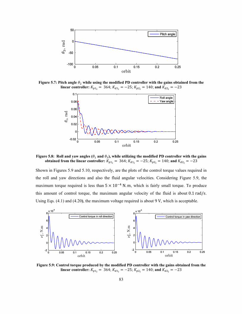
Figure 5.7: Pitch angle 𝜃2 while using the modified PD controller with the gains obtained from the linear controller: 𝐾𝑝1𝑖 = 364; 𝐾𝑑1𝑖 = −25; 𝐾𝑝2𝑖 = 140; and 𝐾𝑑2𝑖 = −23

Figure 5.8: Roll and yaw angles (𝜃1 and 𝜃3), while utilizing the modified PD controller with the gains obtained from the linear controller: 𝐾𝑝1𝑖 = 364; 𝐾𝑑1𝑖 = −25; 𝐾𝑝2𝑖 = 140; and 𝐾𝑑2𝑖 = −23

Shown in Figures 5.9 and 5.10, respectively, are the plots of the control torque values required in

the roll and yaw directions and also the fluid angular velocities. Considering Figure 5.9, the

maximum torque required is less than 5 × 10−4 N. m, which is fairly small torque. To produce

this amount of control torque, the maximum angular velocity of the fluid is about 0.1 rad/s.

Using Eqs. (4.1) and (4.20), the maximum voltage required is about 9 V, which is acceptable.

Figure 5.9: Control torque produced by the modified PD controller with the gains obtained from the linear controller: 𝐾𝑝1𝑖 = 364; 𝐾𝑑1𝑖 = −25; 𝐾𝑝2𝑖 = 140; and 𝐾𝑑2𝑖 = −23

83

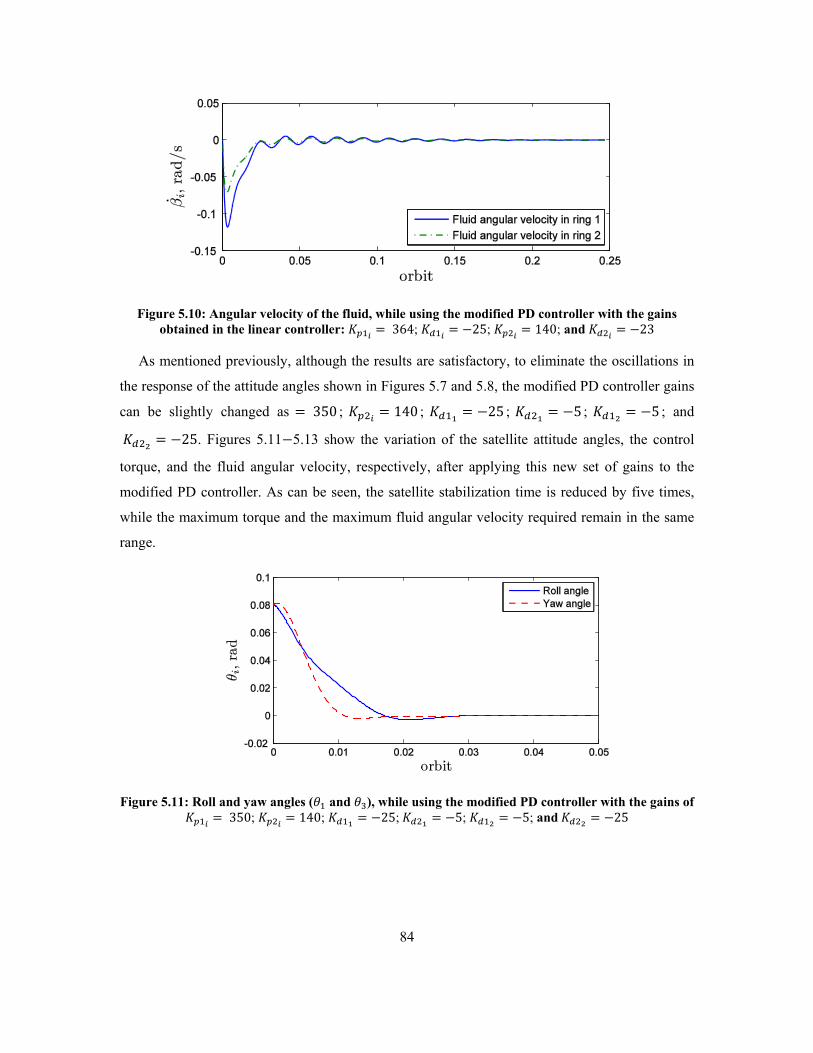
Figure 5.10: Angular velocity of the fluid, while using the modified PD controller with the gains obtained in the linear controller: 𝐾𝑝1𝑖 = 364; 𝐾𝑑1𝑖 = −25; 𝐾𝑝2𝑖 = 140; and 𝐾𝑑2𝑖 = −23

As mentioned previously, although the results are satisfactory, to eliminate the oscillations in

the response of the attitude angles shown in Figures 5.7 and 5.8, the modified PD controller gains

can be slightly changed as = 350 ; 𝐾𝑝2𝑖 = 140 ; 𝐾𝑑11 = −25 ; 𝐾𝑑21 = −5 ; 𝐾𝑑12 = −5 ; and

𝐾𝑑22 = −25. Figures 5.11−5.13 show the variation of the satellite attitude angles, the control

torque, and the fluid angular velocity, respectively, after applying this new set of gains to the

modified PD controller. As can be seen, the satellite stabilization time is reduced by five times,

while the maximum torque and the maximum fluid angular velocity required remain in the same

range.

Figure 5.11: Roll and yaw angles (𝜃1 and 𝜃3), while using the modified PD controller with the gains of 𝐾𝑝1𝑖 = 350; 𝐾𝑝2𝑖 = 140; 𝐾𝑑11 = −25; 𝐾𝑑21 = −5; 𝐾𝑑12 = −5; and 𝐾𝑑22 = −25

84

Figure 5.12: Control torque produced by the modified PD controller with the gains of 𝐾𝑝1𝑖 = 350; 𝐾𝑝2𝑖 = 140; 𝐾𝑑11 = −25; 𝐾𝑑21 = −5; 𝐾𝑑12 = −5; and 𝐾𝑑22 = −25

Figure 5.13: : Angular velocity of the fluid, while using the modified PD controller with the gains of 𝐾𝑝1𝑖 = 350; 𝐾𝑝2𝑖 = 140; 𝐾𝑑11 = −25; 𝐾𝑑21 = −5; 𝐾𝑑12 = −5; and 𝐾𝑑22 = −25

5.5. Summary

In this chapter, the attitude dynamics and control of a spinning satellite using two fluid rings

as attitude actuators were investigated. To obtain a better understanding of the system’s

behaviour, first, a linear dynamical model of this satellite and the fluid rings was developed.

Then, by applying the pole placement method, a controller was designed to asymptotically

stabilize the attitude angles. A similar analysis was carried out using the nonlinear model, where a

modified PD controller was designed to stabilize the satellite dynamics. The same gains as the

ones obtained for the linear feedback controller were used in this modified PD controller. The

performance of the fluid ring actuators was then improved by changing the controller’s gains

85

slightly. The results achieved were satisfactory: the magnitude of the fluid angular velocity

required was acceptably small, while the satellite was stabilized quite fast.

86

Chapter 6

A HYBRID ATTITUDE CONTROLLER CONSISTING

OF ECTROMAGNETIC TORQUE RODS AND A FLUID

RING

To select an appropriate attitude control actuator, one issue to consider is the size of the

satellite. Small satellites are constrained by their mass and the power budget. Moreover, the

stabilizing torque that small satellites require is not so large. Magnetic actuators are appropriate

for the attitude control of small satellites, especially as these actuators are quite light. The

downside of the electromagnetic actuators is that they cannot produce a general three-dimensional

torque. Nevertheless, although slowly, a satellite can be completely stabilized by using two

magnetic coils due to the strong dynamics coupling between the roll and yaw motions. It is shown

in this chapter that adding an active fluid ring to the system of two magnetic actuators will lead to

a faster stabilization.

87

6.1. Dynamics Modeling

To formulate the dynamics model, a LVLH reference frame located at the center of mass of

the satellite is defined, as in Section 2.1 (Figure 2.3): Y0 is perpendicular to the orbital plane; 𝑍0

is directed towards the center of the Earth; and 𝑋0 is defined so as to obtain a right hand

coordinate system. At the equilibrium configuration, the principal axes of the satellite are aligned

with the LVLH reference frame. The orientation of the satellite at any instant is described by

three rotation angles 𝜃1 , 𝜃2 , and 𝜃3 about 𝑋 , 𝑌 , and Z axes of the body frame, respectively.

Moreover, the satellite is considered to have two magnetic coils which produce torques along the

roll and pitch axes as well as a fluid ring whose axis of symmetry is in the yaw direction, as

depicted in Figure 6.1. The center of mass of each coil and the fluid ring is assumed to coincide

with that of the satellite.

Figure 6.1: A satellite with two magnetic coils and one fluid ring

The equations governing the motion of the satellite and the fluid ring are

𝑰𝒔�̇� + 𝝎 × 𝑰𝒔𝝎 = 𝝉𝒈𝒈 + 𝝉𝒄 + 𝝉𝒓 (6.1)

𝑰𝒇��̇� + �̈� + 𝝎 × �̇� � + 𝝎 × 𝑰𝒇�𝝎 + �̇�� = 𝝉𝒈𝒈𝒇 − 𝝉𝒓 − 𝝉𝒑 (6.2)

Equations (6.1) and (6.2) are obtained from Eqs. (2.2) and (2.10) as per the explanation

given hereafter: since there is only one fluid ring in this satellite, the terms ∑ 𝑹𝒊𝝉𝒓𝒊𝑘𝑖=1 are

replaced by 𝝉𝒓 = [𝑚11 𝑚21 𝜏𝑓]𝑇 , where 𝑚11 and 𝑚21 are the reaction moments exerted by

the fluid ring along the roll and pitch directions, respectively. Further, 𝜏𝑓 is the fluid friction

Y

Z

X

Fluid ring

Magnetic

torque rod

88

torque which can be obtained using Eq. (2.16). In Eq. (6.1), the control torque 𝝉𝒄 includes the

torque 𝝉𝒎 produced by the magnetic torquers as well as 𝝉𝒑 = [0 0 𝜏𝑝]𝑇 produced by the

pump of the fluid ring. Further, in Eqs. (6.1) and (6.2), 𝝎 is the angular velocity of the satellite,

�̇� = [0 0 �̇� ]𝑇, where �̇� is the fluid angular velocity. The inertia matrices of the satellite and

the fluid ring are denoted by 𝑰𝒔 and 𝑰𝒇 , respectively. Further, 𝝉𝒈𝒈 and 𝝉𝒈𝒈𝒇 are the gravity

gradient torques exerted on the satellite and the fluid ring, respectively.

As mentioned previously, the attitude control torque in this satellite is produced by two

magnetic coils and one fluid ring. Since magnetic coils cannot produce torque in the direction of

the Earth’s geomagnetic field vector 𝒃, the component of the control torque 𝝉𝒄 parallel to 𝒃

should be produced by the pump pressure; this decomposition method is indeed extracted from a

previous work reported by Forbes and Damaren (2010) . On the other hand, the direction of the

pump pressure torque 𝝉𝒑 is fixed and aligned with the 𝑍 axis of the satellite body fixed frame.

This indicates that only by changing the magnitude of 𝝉𝒑, the parallel component of the control

torque 𝝉∥ can be produced. This is illustrated in Figure 6.2, in which the plane 𝑃 is perpendicular

to the vector 𝒃. The term 𝝉𝒎 is the magnetic torque vector; 𝝉𝒄 = 𝝉⊥ + 𝝉∥, where 𝝉⊥ being the

component of the control torque perpendicular to vector 𝒃.

Figure 6.2: The control torque vector decomposition

The parallel component of the control torque is given by

𝝉∥ = 𝒃�𝒃�𝑻𝝉𝒄 (6.3)

𝝉𝒑

𝝉𝒄

𝝉𝒎

𝝉⊥

𝝉∥

P

b

𝝉𝒑∥

𝝉𝒑⊥

89

where 𝒃� = 𝒃/‖𝒃‖ is the unit vector along the Earth’s geomagnetic field; this is worth mentioning

that in numerical computations, this vector is expressed in the body frame of the satellite. Further,

𝝉∥ = 𝝉𝒑∥ and 𝝉𝒑∥ = 𝒃�𝒃�𝑻𝝉𝒑; hence, Eq. (6.3) can be rewritten as below:

𝒃�𝒃�𝑻𝝉𝒄 = 𝒃�𝒃�𝑻𝝉𝒑 (6.4)

In the above equation, 𝒃�𝑻𝝉𝒄 and 𝒃�𝑻𝝉𝒑 are scalar. Since 𝝉𝒑= [0 0 𝜏𝑝]𝑇, we have 𝒃�𝑻𝝉𝒑 = 𝑏�3𝜏𝑝.

Therefore, the above equation can be simplified as:

𝒃�𝑻𝝉𝒄= 𝑏�3𝜏𝑝 (6.5)

From Eq. (6.5), it can be readily concluded that 𝜏𝑝 = (1/𝑏�3)𝒃�𝑻𝝉𝒄 ; thus, the torque vector

required to be produced by the pump pressure is:

𝝉𝒑 = 1/𝑏�3(𝒃�𝑻𝝉𝒄)[0 0 1]𝑇 (6.6)

Substituting Eq. (6.6) into Eq. (6.2) yields the equation of motion of the fluid ring:

𝑰𝒇��̇� + �̈� + 𝝎 × �̇� � + 𝝎 × 𝑰𝒇�𝝎 + �̇�� = 𝝉𝒈𝒈𝒇 − 𝝉𝒓 − (1/𝑏�3)(𝒃�𝑻𝝉𝒄)[0 0 1]𝑇 (6.7)

Referring back to Figure 6.2, the normal component of the control torque 𝝉⊥ is produced by

the coils and the fluid ring, as per the equation 𝝉⊥ = 𝝉𝒑⊥ + 𝝉𝒎. Knowing that 𝝉∥ = 𝝉𝒑∥, we can

obtain:

𝝉𝒎 = 𝝉𝒄 − 𝝉𝒑 (6.8)

To determine the torque to be produced by each magnetic coil, an orthonormal set of base

vectors 𝒒�𝟏 and 𝒒�𝟐, which spans the plane P, is chosen as follows (Das et al., 2010):

𝒒�𝟏𝑻 = [1 0 −𝑏�1/𝑏�3], 𝒒�𝟐𝑻 = [−𝑏�1𝑏�2/𝑏�3 (𝑏�12 + 𝑏�32)/𝑏�32 −𝑏�2] (6.9)

Defining the matrix 𝑸� = [𝒒�𝟏 𝒒�𝟐], we have

90

𝑸�𝑻𝝉𝒎 = 𝑸�𝑻(𝝉𝒄 − 𝝉𝒑) (6.10)

Now, the relation between 𝝉𝒎 and the magnetic dipole moment vector 𝒎𝒄𝒐𝒊𝒍

= �𝑚𝑐𝑜𝑖𝑙𝑥 𝑚𝑐𝑜𝑖𝑙𝑦 0�𝑇 is recalled from (Wertz, 1999):

𝝉𝒎 = ‖𝒃‖𝒃�×𝒎𝒄𝒐𝒊𝒍 (6.11)

where 𝒃�× is the cross product matrix of 𝒃� defined below:

𝒃�× = �0 −𝑏�3 𝑏�2𝑏�3 0 −𝑏�1−𝑏�2 𝑏�1 0

� (6.12)

Since this system consists of only two coils, 𝒎𝒄𝒐𝒊𝒍 has only two non-zero components. Hence,

Eq. (6.11) can be rewritten as:

𝝉𝒎 = ‖𝒃‖𝒃�×�𝑚𝑐𝑜𝑖𝑙𝑥 𝑚𝑐𝑜𝑖𝑙𝑦 0�𝑇 (6.13)

Therefore, from Eqs. (6.10) and (6.13), one obtains:

‖𝒃‖

⎣⎢⎢⎢⎡ 1 0 −

𝑏�1𝑏�3

−𝑏�1𝑏�2𝑏�3

𝑏�12 + 𝑏�32

𝑏�32−𝑏�2 ⎦

⎥⎥⎥⎤

�0 𝑏�3−𝑏�3 0𝑏�2 −𝑏�1

� �𝑚𝑐𝑜𝑖𝑙𝑥𝑚𝑐𝑜𝑖𝑙𝑦

� = 𝑸�𝑻(𝝉𝒄 − 𝝉𝒑) (6.14)

From Eq. (6.14), the magnetic dipole moment 𝒎𝒄𝒐𝒊𝒍 can be found as:

�𝑚𝑐𝑜𝑖𝑙𝑥𝑚𝑐𝑜𝑖𝑙𝑦

� = (1/‖𝒃‖)

⎣⎢⎢⎢⎡ 𝑏�1𝑏�2𝑏�3

𝑏�12 + 𝑏�32

𝑏�3𝑏�12 + 𝑏�32

𝑏�3− 𝑏�22 0

⎦⎥⎥⎥⎤−1

𝑸�𝑻(𝝉𝒄 − 𝝉𝒑) (6.15)

Substituting back Eq. (6.15) into Eq. (6.13), the magnetic torque can be obtained as:

91

𝝉𝒎 = �0 𝑏�3−𝑏�3 0𝑏�2 −𝑏�1

�

⎣⎢⎢⎢⎡𝑏�1𝑏�2𝑏�3

𝑏�12 + 𝑏�32

𝑏�3𝑏�12 + 𝑏�32

𝑏�3− 𝑏�2 0

⎦⎥⎥⎥⎤−1

𝑸�𝑻(𝝉𝒄 − 𝝉𝒑) (6.16)

Before proceeding to perform simulations, in order to reduce the numerical errors, Eqs. (6.1),

(6.7), (6.15), and (6.16) are non-dimensionalized. To this end, the recalled non-dimensional

angular velocity terms defined in Section 2.1 are:

The non-dimensional form of the governing equations (6.1), (6.7), (6.15), and (6.16) can now be

written as:

where 𝝉�𝒄 is the non-dimensional control torque, 𝝉�𝒈𝒈 and 𝝉�𝒈𝒈𝒇 being the non-dimensional gravity

gradient torque vectors exerted on the satellite and the fluid ring, respectively. The terms 𝑰�𝒔 and

𝑰�𝒇 are the non-dimensional inertia matrices defined in Eq. (2.23).

𝜃𝑖′ ≡ �̇�𝑖/𝑛, 𝜔�𝑖 ≡ 𝜔𝑖/𝑛 , 𝛽′ ≡ �̇�/𝑛 (6.17)

𝑰�𝒔𝝎�′ + 𝝎� × 𝑰�𝒔𝝎� = 𝝉�𝒈𝒈 + 𝝉�𝒄 + 𝝉�𝒓 (6.18)

𝑰�𝒇(𝝎�′ + 𝜷′′ + 𝝎� × 𝜷′ ) + 𝝎� × 𝑰�𝒇(𝝎� + 𝜷′) = 𝝉�𝒈𝒈𝒇 − 𝝉�𝒓 − [0 0 1]𝑇1/𝑏3(𝒃�𝑻𝝉�𝒄) (6.19)

�𝑚�𝑐𝑜𝑖𝑙𝑥𝑚�𝑐𝑜𝑖𝑙𝑦

� =

⎣⎢⎢⎢⎡ 𝑏�1𝑏�2𝑏�3

𝑏�12 + 𝑏�32

𝑏�3𝑏�12 + 𝑏�32

𝑏�3− 𝑏�22 0

⎦⎥⎥⎥⎤−1

𝑸�𝑻(𝝉�𝒄 − 𝝉�𝒑) (6.20)

𝝉�𝒎 = �0 𝑏�3−𝑏�3 0𝑏�2 −𝑏�1

�

⎣⎢⎢⎢⎡𝑏�1𝑏�2𝑏�3

𝑏�12 + 𝑏�32

𝑏�3𝑏�12 + 𝑏�32

𝑏�3− 𝑏�22 0

⎦⎥⎥⎥⎤−1

𝑸�𝑻(𝝉�𝒄 − 𝝉�𝒑) (6.21)

92

6.2. Simulation and Results

For simulations, in Eqs. (6.18)−(6.21), 𝝉�𝒄 is provided by a PID controller with the control law

expressed below:

𝝉�𝒄 = 𝐾𝑝(𝜽 − 𝜽𝒅) + 𝐾𝑑(𝜽′ − 𝜽′𝒅) + 𝐾𝑖 �� 𝜽 𝑑Γ𝑇

0− � 𝜽𝒅 𝑑Γ

𝑇

0 � (6.22)

where 𝜽 = [𝜃1 𝜃2 𝜃3]𝑇, 𝜽𝒅 being the array of desired attitude angles.

The parameters of the arbitrary system assumed for the simulations reported in this section

are identical to those of the system introduced in Section 2.3. For quick reference, a 100 kg

satellite is considered; the inertia matrix of the whole system consisting of the satellite and the

actuators with respect to the body fixed frame located at the center of mass of the satellite is

assumed to be diagonal, the non-zero entries being 𝐼𝑥𝑥 = 24.08 kgm2, 𝐼𝑦𝑦 = 27.08 kgm2, and

𝐼𝑧𝑧 = 13.67 kgm2. Further, a fluid ring with the radius of 0.2 m and the cross-sectional diameter

of 0.02 𝑚 is considered. The relative initial fluid angular velocity is assumed to be zero. It is also

assumed that the satellite travels in a circular orbit at an altitude of 700 km. To study the effect of

the fluid ring on the satellite with two magnetic torque rods, the simulation is performed initially

for the system without the fluid ring. To this end, in Eqs. (6.18), (6.20), and (6.21), 𝝉�𝒑 and 𝝉�𝒓 are

set to zero. The initial attitude angles and their rates are chosen as π/36 rad and 10−4 rad/s,

respectively. The results of the simulation are shown in Figures 6.3 and 6.4.

Figure 6.3: The attitude angles of a satellite using two magnetic coils with PID gains 𝐾𝑝 = 50, 𝐾𝑑 = 60, and 𝐾𝑖 = 1

93

(a)

(b)

(c)

(d)

(e)

Figure 6.4: Torques produced in the satellite using only two magnetic coils with PID gains 𝐾𝑝 = 50, 𝐾𝑑 = 60, and 𝐾𝑖 = 1: (a) Control torque; (b) Torque produced by the magnetic coils in the roll

direction; (c) Torque produced by the magnetic coils in the pitch direction; (d) Torque produced by the magnetic coils in the yaw direction; (e) Magnetic dipole moments

94

From Figure 6.3, it can be noted that the magnetic coils can stabilize the satellite attitude angles

in about four orbits. It is apparent that only 𝝉⊥ is produced by the magnetic coils, which yields a

fairly slow stabilization. Considering Figure 6.4, it can be seen that the plots of the control torque

components have several jumps1. The reason behind this is the singularities of the 2 × 2 matrix in

Eq. (6.21). Indeed, the singular points of the dynamical model of a satellite and magnetic torquers

occur where this matrix loses rank. To cope with this issue, �b�i� = 10−3 is used wherever the

absolute amount of 𝑏�𝑖 becomes less than 10−3.

Figure 6.5: The attitude angles of a satellite using two magnetic coils and one active fluid ring with PID gains 𝐾𝑝 = 70, 𝐾𝑑 = 100, and 𝐾𝑖 = 0

Figures 6.5 and 6.6 show the numerical solutions of the satellite with one active fluid ring and

two magnetic torquers (Eqs. (6.18)− (6.21)) using the same initial conditions and system

parameters as the ones introduced in the foregoing simulation.

As can be seen in Figure 6.5, the satellite stabilization occurs in about one tenth of the orbital

period, while the maximum torque required is less than 2.5 × 10−4 N. m (Figure 6.6). As

explained previously, the fluid ring is in charge of producing the 𝝉∥ component of the control

torque; the maximum torque produced by the fluid ring is 3 × 10−4 N. m. According to Figure

6.6 (a), the maximum value and the trend of 𝝉𝒄 in the roll and pitch axes are quite similar to those

of the magnetic torque plots in these two directions, which are shown in Figure 6.6 (c); it can thus

be concluded that 𝝉⊥ is mainly produced by the magnetic coils. Further, the maximum 𝜏𝑓 is

about 1.5 × 10−5 N. m; a portion of the pump energy is consumed to overcome this friction

torque.

1 The term jump here implies high magnitude peaks of a signal occurring in a short duration of time.

95

(a)

(b)

(c)

96

(d)

(e)

Figure 6.6: Torques produced in the satellite using two magnetic coils and one fluid ring with PID gains 𝐾𝑝 = 70, 𝐾𝑑 = 100, and 𝐾𝑖 = 0: (a) Control torque; (b) Torque produced by the pump; (c) Fluid friction torque; (d) Torque produced by the magnetic coils; (e) Magnetic dipole moments

6.3. Failure Study

Each component used in a satellite is designed for a life span longer than that of the satellite

itself. Nevertheless, to be prepared, performing the failure study of different components of a

satellite is important so as to predict and control the dynamics behaviour of the system, if a failure

condition occurs. In this section, the effect of failure of the fluid ring as well as that of each

magnetic coil is examined.

97

6.3.1. Failure of the fluid ring

A fluid ring can fail due to the failure of its pump. This can lead to two different scenarios: (i)

the pump is jammed and the flow is blocked inside the ring. In this case, the resulting system is

similar to a satellite with two magnetic torque rods without the fluid ring, which was discussed in

Section 6.2. The analysis of this condition revealed that magnetic coils can slowly stabilize the

attitude angles; (ii) the pump is not functional anymore, but the flow is not blocked. This

condition resembles the passive application of the fluid ring; the difference lies in that, in the case

of failure of the fluid ring, the system expects to generate a component of the control torque using

the pump, however in the passive case, the control torque is calculated without counting on the

pump. Therefore, for the case of the failure of the fluid ring, Eqs. (6.18) and (6.19) should be

modified as follows.

𝑰�𝒔𝝎�′ + 𝝎� × 𝑰�𝒔𝝎� = 𝝉�𝒈𝒈 + 𝝉�𝒎 + 𝝉�𝒓 (6.23)

𝑰�𝒇(𝝎�′ + 𝜷′′ + 𝝎� × 𝜷′ ) + 𝝎� × 𝑰�𝒇(𝝎� + 𝜷′) = 𝝉�𝒈𝒈 − 𝝉�𝒓 (6.24)

On the other hand, Eqs. (6.20) and (6.21) remain unchanged. To simulate the performance of this

system, the same initial conditions as what is introduced in the foregoing section are used.

Figure 6.7: Attitude angles of the satellite in the case of failure of the fluid ring with PID gains 𝐾𝑝 =

60, 𝐾𝑑 = 30, and 𝐾𝑖 = 1

Figure 6.7 shows that the attitude angles can be stabilized by the magnetic torque and the

damping effect of the fluid ring. Figure 6.8 (a) shows the control torque required; the maximum

control torque in the yaw direction is 1 × 10−3 N. m. Also, the fluid friction torque, that is the

98

only torque produced in the yaw direction, is quite small, about 5 × 10−7N. m (Figure 6.8 (b)).

Therefore, the damping effect of the fluid is negligible with minor effect on the attitude

stabilization. The maximum magnetic torque in the yaw direction is about 2 × 10−4 N. m

occurring after passing approximately one fourth of the orbital period, as shown in Figure 6.8 (d).

(a)

(b)

99

(c)

(d)

Figure 6.8: Torque produced in the satellite with the fluid ring failure with PID gains 𝐾𝑝 = 60, 𝐾𝑑 = 30, and 𝐾𝑖 = 1: (a) Control torque; (b) Fluid friction torque; (c) Torque produced by the

magnetic coils;(d) Magnetic dipole moments

100

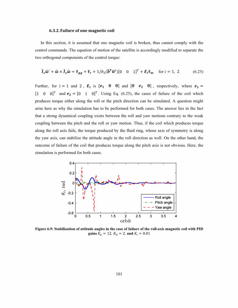
6.3.2. Failure of one magnetic coil

In this section, it is assumed that one magnetic coil is broken, thus cannot comply with the

control commands. The equation of motion of the satellite is accordingly modified to separate the

two orthogonal components of the control torque:

𝑰�𝒔𝝎�′ + 𝝎� × 𝑰�𝒔𝝎� = 𝝉�𝒈𝒈 + 𝝉�𝒓 + 1/𝑏3(𝒃�𝑻𝒖�𝒄)[0 0 1]𝑇 + 𝑬𝒊𝝉�𝒎 for 𝑖 = 1, 2 (6.25)

Further, for 𝑖 = 1 and 2 , 𝑬𝒊 is [𝒆𝟏 𝟎 𝟎] and [𝟎 𝒆𝟐 𝟎] , respectively, where 𝒆𝟏 =

[1 0 0]𝑇 and 𝒆𝟐 = [0 1 0]𝑇 . Using Eq. (6.25), the cases of failure of the coil which

produces torque either along the roll or the pitch direction can be simulated. A question might

arise here as why the simulation has to be performed for both cases. The answer lies in the fact

that a strong dynamical coupling exists between the roll and yaw motions contrary to the weak

coupling between the pitch and the roll or yaw motion. Thus, if the coil which produces torque

along the roll axis fails, the torque produced by the fluid ring, whose axis of symmetry is along

the yaw axis, can stabilize the attitude angle in the roll direction as well. On the other hand, the

outcome of failure of the coil that produces torque along the pitch axis is not obvious. Here, the

simulation is performed for both cases.

Figure 6.9: Stabilization of attitude angles in the case of failure of the roll-axis magnetic coil with PID

gains 𝐾𝑝 = 12, 𝐾𝑑 = 2, and 𝐾𝑖 = 0.01

101

(a)

(b)

(c)

(d)

Figure 6.10: The torque produced in the case of failure of the roll-axis coil with PID gains 𝐾𝑝 = 12, 𝐾𝑑 = 2, and 𝐾𝑖 = 0.01: (a) Control torque; (b) Torque produced by the fluid ring; (c) Torque

produced by the magnetic coils; (d) Magnetic dipole moment in the pitch direction

Figures 6.9 and 6.10 illustrate the results of the failure of the roll-axis coil. Here, to stabilize the

system, the PID gains have to be retuned. The stabilization time is about 4 orbital period;

however, the variations in the roll and yaw angles are large. Considering Figure 6.12 (b), it can be

102

seen that the control torque reaches a value as high as −2 × 10−4 N. m or even 3 × 10−4 N. m at

times. Also, the torque produced by the fluid ring is approximately two times larger than the

control torque about the yaw axis (Figure 6.12 (b)). This shows that the yaw axis of the satellite

almost lies in the plane P of Figure 6.2 to compensate the failure of the roll-axis coil.

Let us now examine the effect of failure of the pitch-axis coil. The plots illustrated in Figures

6.11 and 6.12 show that the system can be stabilized, if the PID gains are retuned. According to

Figure 6.11, the yaw angle varies quite rapidly in the first half of an orbit. The reason behind this

is the weak dynamical coupling between the roll or yaw and the pitch motion. As can be seen in

Figure 6.12 (a), a quite large torque, of about 1.4 × 10−2 N. m, is required in the yaw direction to

stabilize the attitude angles. Indeed, the fluid ring is in charge of producing this torque. It is

noteworthy that, in Figure 6.12 (b), the pump pressure torque reaches the value of 1.4 ×

10−2 N. m at 0.3 orbits (for the sake of illustration the vertical axis of the plot is limited to the

range between −1 × 10−3 N. m and 2 × 10−3 N. m ). The large torque produced by the pump

also affects the pitch angle, as can be seen in Figure 6.11. Moreover, the roll-axis magnetic coil

produces a torque with the maximum value of 1 × 10−3 N. m to stabilize the pitch angle.

Although, in this failure case, a large amount of torque, and hence, a high pump pressure torque

and a high magnetic dipole moment is required (Figure 6.12 (d)), the simulation results prove that

the system still has a chance to remain stable and continue its mission objectives.

Figure 6.11: Stabilization of attitude angles in the case of failure of the pitch-axis coil with PID gains 𝐾𝑝 = 450, 𝐾𝑑 = 15, and 𝐾𝑖 = 0.01

103

(a)

(b)

(c)

(d)

Figure 6.12: Torques produced in the case of failure of the pitch-axis coil with PID gains 𝐾𝑝 = 450, 𝐾𝑑 = 15, and 𝐾𝑖 = 0.01: (a) Control torque; (b) Torque produced by the fluid ring; (c) Magnetic

dipole moment in the roll direction; (d) Torque produced by the magnetic coils

104

6.4. Summary

A novel attitude control system consisting of two magnetic coils and one fluid ring was

proposed in this chapter. The dynamical model of the satellite with two magnetic torque rods and

a fluid ring was developed. Then, the control torque was decomposed into two orthogonal

components. The part of the control torque vector that is parallel to the Earth’s magnetic vector

was considered to be produced by the fluid ring, the rest by the magnetic torque rods. The first

simulation was performed without having the fluid ring in the system. The results showed that the

satellite attitude became asymptotically stable, but slowly. It was found that the stabilization time

can be reduced by a factor of 10 using an active fluid ring; a part of the actuation energy is

consumed to overcome the fluid friction torque. The cases of failure of the fluid ring and one

magnetic torque rod were also examined. In the case of failure of the roll-axis magnetic torque

rod, the variations of the attitude angles were quite high in the first half of the orbit. However, the

attitude angles were finally stabilized. In the case of failure of the pitch-axis coil, the torque

required to be produced by the fluid ring was quite large due to the weak coupling of the pitch

with either the roll or yaw motion. The attitude angles were finally stabilized at the cost of a high

pump pressure torque and a high magnetic dipole moment.

105

106

Chapter 7

CONCLUDING REMARKS AND

RECOMMENDATIONS FOR FUTURE WORK

Satellite attitude can be disturbed because of various natural perturbation sources, such as

the Earth gravity gradient and solar radiation pressure. To avoid this common problem, different

attitude control actuators have been designed so far. Among various control actuators, a novel

type, known as fluid ring actuator, was studied in this thesis; this was motivated by the

perspective of this actuator to produce a high torque to mass ratio. In fact, the goal of this thesis

was the feasibility analysis of using fluid rings as attitude control actuators in satellites and also

finding possible solutions to cope with their drawbacks. In this chapter, a brief summary of the

previous chapters of the thesis is given, while the most significant conclusions of each chapter are

highlighted. At the end, topics of future work to continue this study are proposed.

107

7.1. Summary and Findings

A model was developed in Chapter 2 to describe the three-dimensional attitude dynamics of

a satellite with fluid ring actuators. The model in question can handle two different cases:

satellites with (i) three orthogonal axes; (ii) four fluid rings in a pyramidal configuration. This

mathematical model was used to evaluate the performance of the fluid rings as either a passive or

active method of attitude stabilization. Although the passive application of fluid rings could

stabilize the attitude angles of a satellite in a circular orbit, the simulation results showed that an

asymptotic stability cannot be achieved for the pitch motion of a satellite in an elliptical orbit.

Moreover, the stabilization, when achieved, was fairly slow. Therefore, a PID controller was

designed to use the fluid rings actively so as to stabilize the satellite attitude angles in a

reasonably short period of time. The simulation results confirmed that the satellite attitude can be

effectively controlled by four fluid rings in a pyramidal configuration, if the controller gains are

properly tuned. Further, according to the analysis reported in the thesis, the failure of one fluid

ring in the set of actuators could be tolerated by the three remaining rings without changing the

control law; however, in this condition, the steady state fluid flow rates within the rings did not

vanish even when the satellite was stabilized. This is undesirable due to the unnecessary energy

consumption. A remedy to this problem was found by modifying the control law to contain a

feedback of the fluid angular velocity; the final conclusion was that the fluid ring actuator system

is, in fact, fault-tolerant. Further, the parameter uncertainties were handled by designing a sliding

mode controller, which is robust and compatible with the nonlinearities of the system. This

controller stabilized the attitude angles of the satellite, while considering the parameters

uncertainties in the model to be as large as 15% of their nominal values. The simulation results

showed high chattering in the fluid angular velocities and control torques. To eliminate the

chattering effect, a switching control law consisting of a sliding mode and a PID controller was

developed; the PID is only activated when the error signal becomes smaller than a threshold

value. The new controller performed satisfactorily.

The first experiment conducted was on a single loop fluid ring; this experiment mostly

consists of qualitative tests to observe the system behaviour on a single-axis simulator. The PID

controller of the setup was set to track the fluid angular velocity found from the theoretical

analysis. Indeed, a dynamical model has been developed for a disk carrying a single fluid ring.

The motivation behind developing this model was to obtain numerical results that could be

108

compared to those from the experiments in order to validate the modeling approach. It was noted

that the setup was able to maintain attitude within an acceptable tolerance. The fluid ring setup

has proved the feasibility of attitude control using fluid rings. However, it was noted that, to

produce the desired control torque, the input voltage required to regulate the fluid is fairly high,

more than 12 𝑉.

The experimental validation of the theoretical results obtained for the three dimensional

stabilization was also sought. However, due to various practical issues, such as the defects in the

pumps and the manufacturing of the system, a complete test could not be conducted. Therefore, a

hardware-in-the-loop experiment was performed. The results showed that the system can follow

the control command to produce the fluid flow required for attitude stabilization with quite high

accuracy.

According to the experimental results, producing large torques (higher than 5 × 10−3 N. m)

by fluid rings requires high input voltage (more than 12 𝑉), that may not be easily achievable in

satellites. Hence, the feasibility of using fluid rings as auxiliary actuators combined with other

types of attitude stabilization methods was investigated. In this regard, first, a spinning satellite

with two fluid rings normal to the roll and yaw axes was considered. Designing a controller for

this system with time-varying coefficient in the equations of motion was not straightforward.

Therefore, in order to obtain a preliminary understanding of the system dynamics, simplifying

assumptions regarding the magnitude of the attitude angles were made. Based on these

assumptions, the linear dynamical model of the system was developed, for which a controller was

designed using the pole placement method. The insight obtained from the linear model became

very helpful in the design of a controller for the original nonlinear model. The attitude angles of

the system were stabilized fast, while the effective control torque required was lower than

10−3 N. m. As a second instance of using fluid rings, a new actuation system that includes one

fluid ring with two magnetic torquers was proposed. In order to determine the components of the

stabilization torque to be generated from the fluid ring and the magnetic torquers, the control

torque was decomposed into two components: one parallel to the Earth’s magnetic field vector;

the other its complement. In the case study reported, the control torque needed to be produced by

the fluid ring was less than 2 × 10−3 𝑁.𝑚; the satellite attitude angles were also stabilized within

a short time period. The cases of failure of the fluid ring and each magnetic torquer were also

examined. It was shown that the failure of the fluid ring can be compensated by the two magnetic

109

torquers due to the nonlinear coupling which exists between the roll and yaw motions. However,

the failure of the magnetic torquers, especially the one that produces the torque along the pitch

direction, can cause instability in the satellite orientation. In this case, the attitude angles could be

stabilized via modifying the control law. It is noteworthy that the torque required to be produced

by the fluid ring when one magnetic torquer fails remained below 2 × 10−3 N.m. In conclusion,

it seems that combining the fluid ring actuator with magnetic torquers is the most efficient

application of the former. Indeed, for such system, the controller design is not complex, while the

torque required to be produced by the fluid ring is quite small.

7.2. Recommendations for Future Work

The recommendations for future work are listed below:

i. Three dimensional control validation: The three dimensional control experiment

reported in this thesis was of hardware-in-the-loop experiment type. However,

testing the performance of the fluid rings with a full three dimensional setup

mounted on the simulator can validate the theoretical results more accurately.

ii. Using an observer in the experimental testing: As mentioned in Chapter 4 the

computer used in the experiments was quite limited in terms of computational speed.

This fact did not allow the real time application of the Kalman filter. Therefore, the

online usage of an observer, such as a Kalman filter is recommended for further

experimental work.

iii. Flexibility analysis of the satellite: Considering the satellite as a rigid body is an

acceptable assumption for the feasibility analysis reported in this thesis. However,

there is still room for more accurate modeling and simulations, which can be done

by modeling the satellite as a flexible body.

iv. Considering the interaction of the fluid and the ring: Due to the interaction

between the fluid and the ring, vibrations can be induced into the system, something

which adversely affects the control system. Hence, studying the fluid structure

interaction in the rings is a topic which requires further attention.

110

REFERENCES

Ahmed, J., and Bernstein, D.S. "Adaptive Control of Double-Gimbal Control-Moment Gyro with

Unbalanced Rotor." Journal of Guidance, Control, and Dynamics, 2002: 105-115.

Akiyama, K. "Feedback-Based Time Optimal Control System for Rapid Attitude Maneuver with

Micro Control Moment Gyros." Advances in the Astronautical Sciences, 2010: 91-102.

Ashrafiuon, H., and Erwin, R.S. "Shape Change Maneuvers for Attitude Control of

UnderActuated Satellites." American Control Conference. Portland, OR, USA, June 2005. 895-

900.

Ayoubi, M.A., and Longuski, J.M. "Asymptotic Theory for Thrusting, Spinning-up Spacecraft

Maneuvers." Acta Astronautica, 2009: 810-831.

Barba, P.M., and Aurbrun, J.N. "Satellite Attitude Acquisition by Momentum Transfer." AIAA

Journal, 1976: 1382-1386.

Battagliere, M.L., Fiorillo, F., Ferrara, E., and Santoni, F. "Permeable Rods Ground Testing

System for Cubesat Angular Velocity and Residual Oscillations Damping." 61st International

Astronautical Congress (IAC). Prague, Sept 2010. 2217-2225.

Bolandi, H., Bayat, F., and Nasirian, M. "Attitude Control of Spinning Satellite Subject to

Actuators Restriction Using Eigenstructure Assignment." 1st International Symposium on

Systems and Control in Aerospace and Astronautics. Harbin, Jan 2006. 1413-1419.

111

Chen, M., Zhang, S.J., Liu, F.R., and Zhang, Y.C. "Combined Attitude Control of Small Satellite

Using One Flywheel and Magnetic Torquers." 2nd International Symposium on System and

Control in Aerospace and Astronautics, ISSCAA. Shenzhen, China, Dec 2008. 1-6.

Das, S., Sinha, M., Kumar, K.D., and Misra, A. "Reconfigurable Magnetic Attitude Control of

Earth-pointing Satellite." Journal of Aerospace Engineering, 2010: 1309-1326.

De Ruiter, A. "A Fault-Tolerant Magnetic Spin Stabilizing Controller for the JS2Sat-FF Missin."

Acta Astronautica, 2011: 160-171.

Forbes, J.R., and Damaren, C.J. "Geometric Approach to Spacecraft Attitude Control Using

Magnetic and Mechanical Actuation." Journal of Guidance, Control and Dynamics, 2010: 590-

594.

Fortescue, P., and Stark, J. Spacecraft Systems Engineering. 2nd Edition. England: Wiely, 1995.

Godard, Abreu, N., and Kumar, K.D. "Fault-Tolerant Attitude Control of Miniature Satellite

Using Reaction Wheels." Advances in the Astronatical Sciences, 2010: 159-178.

Hablani, H.B. "Momentum Accumulation Due to Solar Radiation Torque, and Reaction Wheel

Sizing, with Configuration Optimization." AIAA Journal of Guidance, Control, and Dynamics,

1994: 805-814.

Haga, R.A., and Saleh, J.H. "Epidemiology of Satellite Anomalies and Failures: A Subsystem-

Centric Approach." Acta Astronautica, 2011: 676-690.

Horri, N.M., and Palmer, P. "Practical Implemention of Attitude-Control Algorithms for

Underactuated Satellite." Journal of Guidance, Control, and Dynamics , 2012: 40-50.

Hsu, D., Latombe, J.C., and Motwani, R. "Path Planning in Expansive Configuration Spaces."

International Journal of Computational Geometry and Applications, 1999: 495-512.

Hughes, C.P. Spacecraft attitude dynamics. New York: Wiely, 1986.

Huo, X.a, Xiao, B., and Hu, Q. "Adaptive Sliding Mode Attitude Tracking Control for Spacecraft

Under Actuator Misalignment." Journal of South University, 2011: 233-239.

112

Hur-Diaz, S., Wirzburger, J., and Smith, D. "Three Axis Control of the Hubble Space Telescope

Using Two Reaction Wheels and Magnetic Torquer Bars for Science Observations." Advances in

the Astronautical Sciences, 2008: 335-350.

Iskenderian, T.C. "Liquid Angular-Momentum Compensator." NASA Tech Brifes, 1989: 80-85.

Ismail, Z., and Varatharajoo, R. "A Study of Reaction Wheel Configurations for a 3-axis Satellite

Attitude Control." Advances in Space Research, March 2010: 750-759.

Jiang, Y., Yao, Y., and He, F.H. "Scheme of Mass Moment Spacecraft and It's Control Problem."

Systems Engineering and Electronics, 2008: 320-323.

Jin, J., and Hwang, L."Attitude Control of A Spacecraft With Single Variable-Speed Control

Moment Gyroscope." Journal of Guidance, Control, and Dynamics, 2011: 1920-1924.

Kalman, R.E. "A New Approach to Linear Filtering and Prediction Problems." Journal of Basic

Engineering, 1960: 35-45.

Kaplan, M.H. Modern Spacecraft Dynamics & Control. New York: Wiley, 1976.

Kataoka, J., and Kawai, N. "Design of Tokyo Tech Nano-Natellite Cute-1.7+APD II and Its

Operation." Acta Astronautica, 2010: 1412-1424.

Kazinczy, B., and Liebing, L. "Development of a Plasma-Ablation-Accelerator for Satellite

Attitude Control." Dtsch Luft Raumfahrt Forschungsber, 1975.

Kelly, A., McChesney C., Smith P.Z.C., and Waltena S. "A Performance Test of a Fluidic

Momentum Controller in Three Axes." NASA Technical Report, May 2004.

Kennel, H.F. "A Control Law for Double-Gimballed Control Moment Gyros Used for Space

Vehicle Attitude Control." NASA Report, TM-64536, 1970.

Kim, E., Bang, H., and Lee, S.H. "Attitude-Independent Magnetometer Calibration Considering

Magnetic Torquer Coupling Effect." Journal of Spacecraft and Rockets, 2011: 691-694.

Kowalchuk, S.A., and Hall, C.D. "Spacecraft Attitude Sliding Mode Controller Using Reaction

Wheels." AIAA/AAS Astrodynamics Specialist Conference and Exhibit. Hawaii, Aug 2008.

113

Krishnan, S., and Vadali, S.R. "An Inverse-Free Technique for Attitude Control of Spacecraft

Using CMGS." Acta Astronautica, 1996: 431-438.

Kumar K.D. "Satellite Attitude Stabilization Uing Fuid Rings." Acta Mechanica, January 2009:

117-131.

Kurokawa, H. "Constrained Steering Law of Pyramid-Type Control Moment Gyros and Ground

Tests." Journal of Guidance, Control, and Dynamics, 1997: 445-449.

Kusuda, Y., and Takahashi, M. "Design of Feedback Control System Using Nominal Inputs for

Satellite Attitude Maneuver Using Control Moment Gyros." AIAA Conference of Guidance,

Navigation, and Control. Chicago, Aug 2009.

Kwakernaak, H., and Sivan, R. Linear Optimal Control Systems. New York: Wiley, 1972.

Lappas, V., and Wie, B. "Robust Control Moment Gyroscope Steering Logic with Gimbal Angle

Constraints." Journal of Guidance, Control, and Dynamics, 2009: 1662-1666.

Larson, W.J., and Wertz, J.R. Space Mission Analysis and Design. Kluwer Academic Publishers,

1992.

Laughlin, D.R., Sebesta, H.R., and Ckelkamp-Baker, D.E. "A Dual Function Magneto

Hydrodynamic (mhd) Device for Angular Motion Measurement and Control." Advances in the

Astronautical Sciences, 2002: 335-348.

Lee, H., Kim, Y., Cheon, Y.J., and Kim, H.S. "Reconfigurable Satellite Attitude Control Scheme

Using Two Reaction Wheels for Limited Mission." 60th International Astronautical Congress

(IAC). Daejeon, Sept 2009. 4934-4944.

Leeghim, H., Lee, D., Bang, H., and Lee, K. "Spacecraft Attitude Control by Combination of

Various Torquers." International Journal of Systems Science, 2009: 995-1009.

Leeghim, H., Bang, H., and Park, J.O. "Singularity Avoidance of Control Moment Gyros by One-

Step Ahead Singularity Index." Acta Astronautica, 2009: 935-945.

Leimanis, E. The General Problem of the Motion of Coupled Rigid Bodies About a Fixed Point.

New York: Springer-Verlag, 1965.

114

Li, F., and Bainum, P.M. "Numerical Approach for Solving Rigid Spacecraft Minimum Time

Attitude Maneuvers." Journal of Guidance, Control, and Dynamics, 1990: 38-45.

Li, J., and Kumar, K.D. "Fault Tolerant Synchronization Control During Formation Flying."

Journal of Aerospace Engineering, 2011: 251-263.

liu, H., Wanng, H., Feng, C., and Ye, W. "Attitude Control of Micro Satellite Using Thruster Plus

Bias Momentum Wheel." ICIC Express Lertters, 2010: 1269-1274.

Lurie, B.J., and Schier, J.A. "Liquid-Ring Attitude-Control System for Spacecraft." NASA Tech

Briefs, 1990: 82.

Lurie, B.J., Schier, J.A., and Iskenderian, T.C. Fluid-Loop Reaction System. US Patent 5026008.

1991.

Maeda, K., Hidaka, T., and Uo, M. "A Magnetic Libration Control Scheme for Gravity-Gradient

Stabilized Small Satellite." Advances in the Astronautical Sciences, 1997: 887-8896.

Marshall, T., Gunderman, T., and Mobley, F. "Reaction Wheel Control of the MSX Satellite."

Advances in the Astronautical Sciences, 1991: 119-138.

Martinellia, M.I. and Sanchez, P.R.S. "Passive 3 Axis Attitude Control of MSU-1 Pico-Satellite."

Acta Astronautica, 2004: 507-518.

Maynard, R.S. Fluid Momentum Controller. US Patent 4776541. Oct. 11, 1988.

McMahon, J., and Schaub, H. "Simplified Singularity Avoidance Using Variable Speed Control

Moment Gyroscope Null Motion." Advances in the Astronautical Sciences, 2010: 1611-1623.

Nanamori, Y., Takahashi, M., Tanikimi, S., Yoshida, K., and Ohkani, Y. "Singularity Avoidance

of Control Moment Gyros Using Optimization of Initial Gimbal Angles and Application to Multi

Target Pointing for Satellite Attitude Control." Advances in the Astronautics Sciences, 2008:

2337-2352.

Navabi, N., and Nasiri, N. "Three-axis Stabilization of a Low Earth Orbit Spacecraft Utilizing

Magnetorquers and Reaction Wheels Combinations, According to Energy Consumption." 61st

International Astronautical Congress. Prague, Sept 2010. 4769-4777.

115

Ogata, K. Modern Control Engineering. 5. New York: Prentice-Hall, 2009.

Patel, S., and Kumar, K.D. Design and Development of Fluid Based Attitude Control System.

Technical Report, Toronto, Canada: Ryerson University, 2010.

Raus, R., Gao, Y., and Watt., M. "Review and Analysis of Single-Thruster Attitude Control

Techniques for Spinning Spacecraft." 61st International Astronautical Congress (IAC). Prague,

Sept 2010. 3358-3369.

Richie, D.J., and Lappas, V.J. "Saving Mass in Optimally Sizing a Small Satellite Energy Storage

and Attitude Control System." Advances in the Astronautical Sciences, 2007: 1161-1177.

Sands, T.A., Kimz, J.J., and Agrawal, B. "Control Moment Gyroscope Singularity Reduction Via

Dicoupled Control." IEEE Southeastcon. Atlanta, March 2009. 388-391.

Schaub, H., and Junkins, J.L. Analytical Mechanics of Space Systems. Reston, Virginia: AIAA

Education Series, 2003.

Shames, H. I. Mechanics of Fluids. New York: McGraw-Hill, 1992.

Slotine, J.J., and Weiping, L. Applied Nonlinear Control. 1st Edition. New Jersey: Englewood

Cliffs, 1991.

Sofyali, A., and Jafarov, E.M. "Three-axis Attitude Control of a Small Satellite by Magnetic Pd-

like Controller Integrated with Passive Pitch Bias Momentum Method." 5th International

Conference on Recent Advances in Space Technologies. Istanbul, Turkey, June 2011. 307-331.

Srikant, S., and Akella, M.R. "Persistence Filter Based Attitude Stabilization of Micro Satellites

with Variable Amplitude Thrusters." Advanced in the Astronautical Sciences, 2010: 649-659.

Stenmark, L., and Lang, M. "Micro Propulsion Thrusters and Technologies." European Space

Agency, (Special Publication) ESA SP, 1997: 399-405.

Steyn, W.H. "Fuzzy Control for a Non-Linear MIMO Plant Subject to Control Constraints." IEEE

Transactions on Systems, Man and Cybernetics, 1994: 1565-1571.

Sun, Z., Yang, X., and Yang, D. "Active Magnetic Control Methods for Small Satellite." Journal

of Aerospace Engineering, 2003: 38-44.

116

Tang, H.B., Zi, Z.P., Jin, X., Jiang, J., Zau, Y., and Yan, Z.Y. "A Micro-Propulsion System with

Propane Propellent for Small Satellite." Advanced Science Letters, 2011: 2015-2021.

Terui, F., Kimura, S., Nagai, Y., Yamamoto, H., Yoshiharo, K., Yamamoto, T., Nakasuka, S.

"Moon Tracking Attitude Control Experiment of A Controlled Bias Momentum Micro Matellite."

AIAA Guidance, Navigation, and Control Conference. San Francisco,California, Aug 2005. 1587-

1601.

Topland, M.P., and Gravdahl, J.T. "Nonlinear Attitude Control of the Micro-satellite ESEO."

55th International Astronautical Federation. Vancouver, Canada, Oct 2004. 757-767.

Tsiotras, P., Shen, H., and Hall, C. "Satellite Attitude Control and Power Tracking with

Energy/Momentum Wheels." Journal of Guidance, Control, and Dynamics, 2001: 23-34.

Vadali, S.R., and Junkins, J. "Optimal Open-Loop and Stable Feedback Control of Rigid

Spacecraft Attitude Maneuvers." Journal of the Astronautical Sciences, 1984: 105-122.

Wang, P., Zheng, W., Zhang, H., and Wu, Z. "Attitude Control of Low-orbit Micro-satellite with

Active Magnetic Torque and Aerodynamic Torque." International Symposium on Systems and

Control in Aeronautics and Astronautics. Harbin, China, June 2010. 1460-1464.

Wertz, J.R. Spacecraft Attitude Determination and Control. Netherlands: Academic Publishers,

1999.

Wie, B. Space Vehicle Dynamics and Control. Reston, Virginia: AIAA Education Series, 1998.

Ye, D., Zhaowei, S., and Shunan, W. "Hybrid Thrusters and Reaction Wheels Strategy for Large

Angle Rapid Reorientation with High Precision." Acta Astronautica, 2011: 149-155.

Zhang, S.F., Qian, S., and Li, P.K. "Study on the Minimal Energy Maneuvering Control of a

Rigid Spacecraft with Momentum Transfer." Journal of Astronautics, 2009: 1504-1515.

117