Embed Size (px)
Citation preview

Algebraic Hierarchical Decomposition of Finite State Automata -A Computational
Approach
Attila Egri-Nagy
A thesis submitted in partial fulfillment of the requirements of the University of Hertfordshire
for the degree of
Doctor of Philosophy The programme of research was carried out in the School of
Computer Science, Faculty of Engineering and Information Sciences University of Hertfordshire.
November 11,2005

To the first human, who took a piece of stone and used it as a tool

Acknowledgments
I would like to thank my supervisors, Chrystopher Nehaniv for showing the amusements of doing mathematics together while moving from a restaurant to a cafe and back to a restaurant again endlessly, Bruce Christianson for his laconic but powerful comments, Pal D6m6si for helping my way into an academic caxeer.
I also would like to thank my 'transitive' supervisor, John Rhodes for giving us enough interesting questions to think about.
I would like thank all the kind people closely around me, who might have found it strange and probably annoying when I was immersed in the world of mathematical symbols.
Finally I would like to thank my violin, a Strad model from Transylvania, for using different neurons in my brain, giving a rest for the parts occupied with mathematics.
ATTILA EGRI-NAGY

Abstract
The theory of algebraic hierarchical decomposition of finite state automata is an important and well developed branch of theoretical computer science (Krohn-Rhodes Theory). Beyond this it gives a general model for some important aspects of our cognitive capabilities and also provides possible means for constructing artificial cognitive systems: a Krohn-Rhodes decom- position may serve as a formal model of understanding since we comprehend the world around us in terms of hierarchical representations. In order to investigate formal models of understanding using this approach, we need efficient tools but despite the significance of the theory there has been no computational implementation until this work.
Here the main aim was to open up the vast space of these decompositions by developing a computational toolkit and to make the initial steps of the exploration. Two different decomposition methods were implemented: the VuT and the holonomy decomposition. Since the holonomy method, unlike the VUT method, gives decompositions of reasonable lengths, it was chosen for a more detailed study.
In studying the holonomy decomposition our main focus is to develop techniques which enable us to calculate the decompositions efficiently, since eventually we would like to apply the decompositions for real-world prob- lems. As the most crucial paxt is finding the the group components we present several different ways for solving this problem. Then we investigate actual decompositions generated by the holonomy method: automata with some spatial structure illustrating the core structure of the holonomy de- composition, cases for showing interesting properties of the decomposition (length of the decomposition, number of states of a component), and the decomposition of finite residue class rings of integers modulo n.
Finally we analyse the applicability of the holonomy decompositions as formal theories of understanding, and delineate the directions for further research.

PAGE
NUMBERING
AS ORIGINAL

Contents
1 Introduction 1.1 The Concept ...........................
1.1.1 Models .......................... 1.1.2 Decompositions ...................... 1.1.3 Hierarchies ........................ 1.1.4 Coordinate Systems ................... 1.1.5 Aspects Do Matter ....................
1.2 The Substrate ........................... 1.2.1 Automata ......................... 1.2.2 Semigroups ........................ 1.2.3 Emulation ......................... 1.2.4 Finiteness, Computational Complexity
1.3 Research Questions and Motivations ..............
1.3.1 Feasibility ......................... 1.3.2 Exploration and Exploitation
.............. 1.3.3 Formal Models of Understanding ............
1.4 Roadmap .............................
2 Mathematical Preliminaries and Notations 2.1 Semigroups and Groups .....................
2.1.1 Semigroups ........................ 2.1.2 Groups .......................... 2.1.3 'kansformations and Permutations ........... 2.1.4 Green's Relations ..................... 2.1.5 Homomorphisms ..................... 2.1.6 Words and the Free Semigroup ..............
2.2 Finite State Automata ...................... 2.3 Wreath Product ......................... 2.4 Examples .............................
2.4.1 Faces of an Automaton ................. 2.4.2 Building a Modulo 4 Counter Hierarchically
2.5 Summary .............................
1 1 1 2 2 3 3 4 4 4 4 5 5 5 6 6 7
8 8 8 9 9
10 10 11 12 12 15 15 17 18
viii

3 The Krohn-Rhodes Theory 19 3.1 The Prime Decomposition Metaphor
.............. 19 3.2 The Building Blocks ....................... 20 3.3 Wiring the Components
..................... 20 3.4 The Krohn-Rhodes Prime Decomposition Theorem ...... 21 3.5 Historical Remarks
........................ 21 3.6 Summary ............................. 22
4 The VU T-technique 23 4.1 The Iterative Construction ................... 23 4.2 Results ............................... 25
4.2.1 The Full Transformation Semigroup .......... 25 4.2.2 More Extreme Examples ................. 25
4.3 Summary ............ 4................ 26
5 The Holonomy Decomposition 27 5.1 Holonomy Decomposition Theorem
............... 27 5.2 Relations of the Extended Set of Images ............ 28
5.2.1 The Extended Set of Images ............... 29
5.2.2 Inclusion ......................... 29 5.2.3 Image Relation ...................... 29 5.2.4 The Subduction Relation and the Skeleton ...... 29 5.2.5 Equivalence Classes ................... 30 5.2.6 Tiles and Tiling ..................... 30 5.2.7 Tile Chains ........................ 31 5.2.8 Height of a Subset .................... 31
5.3 Components ............................ 31 5.3.1 Holonomy Groups .................... 31 5.3.2 Holonomy Permutation-Reset Transformation Semi-
groups ........................... 32 5.4 Mappings on _T .......................... 32
5.4.1 Isomorphisms of Holonomy Groups within a Subduc- tion Equivalence Class
.................. 32 5.4.2 Moving within an equivalence class ........... 34
5.5 Lifting the State Set ....................... 35 5.5.1 Successive Approximation of States ........... 35 5.5.2 Lifting the States ..................... 36
5.6 Lifting the Semigroup ...................... 36 5.6.1 Lifting Transformations ................. 36 5.6.2 Verifying the division .................. 37 5.6.3 Dependency Functions .................. 39 5.6.4 The Circuitry of the Wreath Product .......... 39
5.7 Examples ............................. 40
5.7.1 The Tricks of Tiling ................... 40

5.7.2 Cross Level Tiles ..................... 41 5.7.3 Nonimage Tiles ...................... 42 5.7.4 Strict Subduction for Sets with the Same Cardinality 43 5.7.5 Tile Chains ........................ 43
5.8 Summary ............................. 45
6 Implementational Details of the HolonoMY Decomposition 46 6.1 Related Software Packages .................... 46 6.2 Representational Issues ..................... 47 6.3 'Mvial Implementation Using Brute Force Enumeration
... 48 6.4 Examples ............................. 49
6.4.1 Generating Images .................... 49 6.4.2 Deciding Subduction Relation
.............. 50 6.4.3 Holonomy Components
................. 50 6.5 Visualization ........................... 51 6.6 Summary ............................. 52
7 Constructing Holonomy Components 54 7.1 The Problem ........................... 54
7.1.1 Examples ......................... 55
7.2 Word Based Construction Method ............... 55
7.2.1 Cycles in Automata ................... 55
7.2.2 Graphically Cycle-Free Automata ............
56 7.2.3 Algebraically Cycle-Free Automata
........... 57
7.2.4 Non-Aperiodic Automata ................
59 7.2.5 The Algorithm
...................... 62 7.2.6 Examples
......................... 63 7.3 Dependency Function Based
................... 64
7.3.1 The Algorithm ......................
67 7.3.2 Example
.......................... 68
7.4 Summary ............................. 71
8 Applications 72 8.1 Understanding the Holonomy Decomposition ......... 73
8.1.1 Decompositions Without any Hierarchical Dependence 73 8.1.2 The Role of Subduction Equivalence Classes
...... 73 8.2 Properties of the Holonomy Decomposition .......... 76
8.2.1 Number of Hierarchical Levels ............. 76 8.2.2 Size of a Component's State Set ............ 77
8.3 Decomposition of the Rings of Integers Modulo n....... 79 8.3.1 Representation ...................... 79 8.3.2 The Extended Set of Images ............... 79 8.3.3 Subduction, Equivalence Relation, and the Tiling Pic-
ture ............................ 80

8.3.4 Number of Levels ..................... 82 8.3.5 Number of States ..................... 82 8.3.6 Holonomy Group Components ............. 83 8.3.7 The Lesson ........................ 85
8.4 Formal Models of Understanding ................ 85 8.4.1 Representations in Artificial Intelligence ........ 86 8.4.2 The 'What to doT Problem ............... 86 8.4.3 Capturing Learning ................... 91
8.5 Summary ............................. 92
9 Achievements and Future work 93 9.1 Contributions to Knowledge ................... 93 9.2 Possible Future Research Directions .............. 94 9.3 Exploring a New Landscape ................... 95
A Decompositions of Finite Residue Class Rings of Integers Modulo n, up to n= 20 97
B Dilworth's Theorem
C Related Publications
99
100
Software Architecture 102 D. 1 Grasp ............................... 102 D. 2 jGrasp ............................... 102
E Glossary of Symbols 104

Chapter I
Introduction
For any finite system a working hierarchical model can be generated auto- matically.
If we would like to summarize the main theme of this work very shortly, then we could say that it investigates what the last issue of the previous statement mentions: here we give actual algorithms for generating hierar- chical models, and once we have the computational tools, we generate models for some particularly interesting finite systems. The statement above has been known to be true for a long time [KR65], so our task is only to start using this result. But this is still a long story.
1.1 The Concept
1.1.1 Models
"The best material model of a cat is another, or preferably the same, cat. " A. Rosenblueth [with Norbert Wiener], Philosophy of Science 1945.
What is a model of something? Abstractly speaking, the model is any system which is not thing itself, but it shows some relevant features of the thing or phenomenon to be modeled. In some respect the model should be
easier to handle otherwise the thing could be its own model, (and a map with scale 1: 1 is pretty useless). By a working model we mean that not just the static structure of the original phenomenon is captured, but the model can contain processes as well. Building a model of a system usually involves the identification of its subsystems and their relations. Therefore, the problem of decomposition naturally arises here.
1

Chapter 1. Introduction
1.1.2 Decompositions
Despite some relatively new scientific approachesl, scientific understand- ing still proceeds by taking apart things, identifying their components. Molecules are built up from atoms, atoms from elementary particles, a hu- man brain contains billions of neuron cells, a piece of software is written as code lines of many instructions, etc. By listing the components, we can get to know what are the ingredients for building a given system. Therefore the usefulness of a decomposition method does not need any other justifica- tion. But as we go further during a scientific research, the next and more important question is that how those components are put together, how the subsystems are related to each other. We will show that the actual way of wiring the components together is more interesting than the list of the com- ponents, and this fact is often neglected. Here we emphasize the usefulness of hierarchical compositions, but this needs some justification.
Hierarchies
We comprehend the world around us in terms of hierarchical representa- tions. We recognize social relations, the structure of organizations by the ranking of the members according to some order [Sim96]. We study the phys- ical world along the spatial and size hierarchies from string theory to the galaxies. Software development methodologies like object-orientation struc- ture for computer programs use the hierarchies of both data and procedures [Boo9l). Our decimal base number notation system is also inherently hier- archical. Even the current debate on the definition of emergence revolves around the notion of hierarchical levels. It is beyond question that among our cognitive models hierarchies are pervasive. One might say that this is a constraint on our cognition albeit a very fruitful one, thanks to the nice properties of hierarchies:
information flow between levels are restricted enabling modularity (also within one level with parallel components).
9 generalization and specialization are natural operations realized by taking subsets of levels in either direction up or down the hierarchy.
It's not the case that all systems are hierarchical', rather the opposite is true. Natural systems have tangled hierarchies, hierarchies with strange loops: "The Strange Loop phenomenon occurs whenever, by moving up- wards (or downwards) through the levels of some hierarchical system, we unexpectedly find ourselves right back where we started" (Hof79]. But even
'A nice example is the notion of emergence, where the system is understood by de- scribing simple low-level rules that spontaneously lead to complex behavior [Joh0l].

3
in those cases in understanding them we first use a hierarchical way then we introduce the strange loops as a deviation from hierarchies.
We will not consider the philosophical question here, whether hierarchies are out there in reality or are they just guiding principles of our minds when comprehending the world around us. For the sake of simplicity here it is enough to assume the latter proposition only.
Coordinate Systems
By a coordinate system we mean a notational system (in the broadest possi- ble sense), with which we can address the components and their relations in a decomposition, thus gaining a convenient way for grasping the structure of the original phenomenon. An obvious example is the Descartes coordi- nate system, where we can uniquely specify any point of the n-dimensional space by n coordinates. However, this is an example of an inherently non- hierarchical coordinate system for a totally homogenous system. In general different coordinates have different roles, addressing parts of the system different in size, function, etc. The natural example of a hierarchical coor- dinate system is our decimal positional number notation system: different coordinates correspond to different magnitudes.
Here we consider coordinate systems that are hierarchical and alge- braically produced for and from a finite state automata.
1.1.5 Aspects Do Matter
Things can be described in several forms. Each form represents the same structure but from a different viewpoint and from each distinct viewpoint something else can be seen. Just as walking around a building may support a deeper understanding of it. What is the building for? How big is it? How many people axe in there? Examining several sides may shed light even on the inner structure. It might happen that we do not gain any new information from a different aspect so the different point of views vary in their usability in this respect. Moreover, for different purposes they have different values. For example you can enter the building on the front but not on the rear side. Using different approaches, evaluating them on the base of current purposes, motivations, switching between them - these are probably deeply in our cognitive structure.
It is beyond question that in mathematics these techniques are basic. Given a mathematical structure which is hard to study but it can be mapped to an another domain of well-known constructions, this way the problem is almost solved.

Chapter 1. Introduction
1.2 The Substrate
1.2.1 Automata
Regarding the nature of the models discussed here we have a restriction: they should be described as finite state automata. We claim that this is not really a constraint. Automaton is a concept which is general enough to grasp many interesting phenomena of the world around us. Anything which has states and changes its current state responding to external input can be considered as an automaton.
Many phenomena fit into this scheme: organisms responding quickly to the changes of the environment, chemical reactions, many aspects of real computers, especially language processing, and so on. The wide applicability is due to the very strong abstraction which focuses on the very important notion of change [Ash56].
1.2.2 Semigroups
Groups are mathematical structures capturing the notion of symmetry (re- versible processes, or operations that can be undone). Algebraically semi- groups are the generalization of the concept of the group. Semigroups can capture irreversibility as well, not just symmetry like groups, i. e. there can be operations that cannot be undone. The only one requirement is that the passage of time should be preserved by the associativity of the operation.
In this work the role of the sernigroups is that they are the algebraic aspects of automata: the input symbols of an automaton can be considered as transformations of the state set, as functions. Therefore we can use the precise mathematical tools available in algebra for studying the phenomena being described as an automaton. Philosophically, this aspect also gives us a very nice level of abstraction for computational structures: we can consider processors and memory as the very same resource, since they are not distinguished in the semigroup.
1.2.3 Emulation It should not be surprising that in general, when we decompose something, i. e. identify its components and determine the rules how to put them to- gether, finally we do not get back exactly the same thing. If it is "smaller", then we got the decomposition wrong (or we can say that we have an ap- proximation), if it is "bigger" in some sense, then we talk about emulation.
Emulation is an easy concept in computer science: a machine A2 emu- lates Ai if A2 can do everything what A, can do. It might be able to do
more, but we should be able to use A2 instead of Al in any case. Clearly, it is an important issue how to interpret certain operations of
A2 as the operations of Al. We will consider this in full detail. In alge-
5
braic terms, this will be done by the mappings of the homomorphism from subautomaton for establishing the division (emulation), see Section 2.1.5.
1.2.4 Finiteness, Computational Complexity
Here we deal only with finite structures, but this does not mean that the theory is unable to deal with infinite structures (e. g. [Neh92]). We have the restriction, since we focus on computational implementations and applica- tions of the theory.
Our computers are finite, plants, animals are finite and we humans are also finite in time and in space as well. The actual loss we have is the pathol- ogy of infinite machines only (many uncomputable functions and undecid- able problems). Of course the argument is right that a Turing-machine has more computational power than a finite-state machine or a stack-machine. But let's consider the case of palindromes. In reality we do not have to deal with palindromes with arbitrary length, and if words to be checked are finite then we can tackle the recognition problem with a finite-state machine.
If we stay within the finite realm, we still have serious difficulties. Cal- culating a decomposition is not a simple task, and at every stage of the algorithm, combinatorial explosions may come up. But there is some hope due to the following considerations:
For practical purposes we need a reasonably good decomposition, not the most optimal (e. g. the shortest possible) one.
There might be domains of interesting special problems which admit an efficiently calculable decomposition.
We can use only approximations (not fully calculating all the hierar-
chical levels).
Unfortunately we cannot entirely get rid of undecidable problems even in the* finite case. For example the potential divisibility in finite semigroups is undecidable [KS981.
1.3 Research Questions and Motivations
1.3.1 Feasibility
Our very first question is more than obvious: Is it really possible? Can we calculate such decompositions? Clearly, in the 60's the available computa- tional power of computers was not enough for a challenge like this. But today's computers are more powerful, and the software development tools and computer algebra systems give a lot of help in attacking difficult prob- lems. At least it is time to try.

Chapter 1. Introduction
There is another issue which makes this work timely. Being a mathe- matician and being a computer scientist (or a programmer), though they are quite close to each other, still require different mind sets. Proving that a given mathematical object exists concludes the work of the mathematician, but that is exactly the beginning of the work of the programmers, since that given element should be found possibly in a very huge set.
So our first research issue stated precisely is the following:
0. It is necessary to investigate the computational feasibility of the de-
composition algorithms in order to develop the required software. This requires the comparison and evaluation of different decomposition meth- ods.
The ordinal number 0 here emphasizes that the computational tool for decompositions is not the end product of this work, rather a prerequisite for the actual research.
1.3.2 Exploration and Exploitation
Once we have the computational tool, we can analyse such decompositions that are otherwise not available by manual calculations. Thus, we can start a systematical exploration of specific classes of finite state automata.
1. Study interesting examples for gaining knowledge about the nature of automatically generated decompositions.
The improvement of the decomposition algorithms also remains in focus, since we assume that the more we know about an algorithm the better we can perform.
2. How can we use theoretical insights gained in the exploration phase for improving the decomposition methods?
1.3.3 Formal Models of Understanding
We mentioned before that a cascaded decomposition can be considered as a coordinate system for understanding a given phenomenon. Possible applica- tions of this idea pop up in all different fields where we deal with hierarchical models of systems: physics, where the top leve12 coordinates can be consid- ered as conserved quantities of the system, while the symmetries comprise the bottom level [Rho7l]. In software-development the formal models of understanding might provide tools for automated programming, since de-
veloping a piece of software is just creating a sophisticated cognitive model
'There is an ambiguity between the different meanings of top and bottom level, here we refer the most independent level as top.

7
[Neh94]. In artificial intelligence [Neh96aj embodied agents equiped with the ability of creating formal models from data coming from their sensors could change their representation of the environment on the fly having a great advantage over purely reactive agents or agents with fixed representations. Recently biological sciences produce a huge amount of data that remain largely uninterpreted so far. As a prominent example one might mention the hype around the sequencing of the human genome, which, while undoubtly representing great progress, comprises a big finite description that we only partially understand. In evolutionary biology it is still contentious how complexity changes in the course of evolution. This is due to the unclarified notions of complexity, which can be clearly defined in terms of hierarchical decompositions [NROO].
This short summary of possible applications shows that this research is not only motivated but that even the prospects for the near future results could potentially be highly rewarding. Therefore our final research question, which is only partially answered here is the following.
3. How can we use a cascaded decomposition as a coordinate system providing a formal model of understanding?
1.4 Roadmap
The first chapter introduced the fundamental notions needed for understand- ing this research. The definitions here are very informal, they stay at a very abstract, almost philosophical level, but they should help in understanding the details of what follows.
Chapter 2 presents the mathematical background and fixes the notation used in subsequent chapters.
Chapter 3 briefly introduces the Krohn-Rhodes Prime Decomposition Theorem, which is the basis of this work.
Chapter 4 describes an iterative proof technique for the Krohn-Rhodes Theorem, the VUT technique, and discusses its applicability for practical problems.
Chapter 5 contains the full proof of the Holonomy Decomposition The-
orem. Chapter 6 discusses the general details of a computational implementa-
tion for the holonomy decomposition. Chapter 7 deals with the main problem of constructing the holonomy
components. It describes two different methods for solving the problem. Chapter 8 shows some preliminary applications of the computational
tool. Chapter 9 summarizes the achievements and delineates the possible di-
rections for future research. Wherever it makes sense, there is a section with illustrative examples.

Chapter 2
Mathematical Preliminaries and Notations
"Let no one unversed in geometry enter here. " Written over the gate of Plato's Academy.
Here we establish the close connection between finite state automata and semigroups. The related notions, division and emulation, wreath and cascaded product, etc., show that automata and transformations are just the two different sides of the same coin. For the sake of brevity, only those notions are defined which are needed for the proofs in this work, for more details see [DN05, Arb68, DIM].
The notation applied here is slightly different compared to previous works. We tried to change it for the better, to promote understanding. We use lowercase letters for elements of sets, capital letters for sets, and calligraphic letters for sets of sets or for relations.
We denote the set of integers 10,1, ..., n- 1} by n.
2.1 Semigroups and Groups
Semigroups
A semigroup is a set S equipped with an associative binary operation y: SxS --+ S. Instead Of A(Sl 9 S2) we write SPS2 or more briefly sl S2. If A and B
are subsets of a semigroup, then AB means the set lab: aEA, bE B}. An
element 1 is the identity element of S if sl = ls = s, Vs E S. The identity is
unique if it exists. By S1 we denote S if it has an identity otherwise SUI 1}. By SI we mean SUI I} where I is a new element that acts as an identity on S and itself, the identity of S (if it exists) ceases to be an identity as it fails
on L An element rES is called a right-zero element of S if sr = r, for all
sES. Symmetrically, tES is a left-zero element if is = f, for all sCS. In
addition, oES is the zero element if os = so = o, Vs E S. The zero element
8

9
is also unique if it exists. The order of a semigroup S is its cardinality ISI. We say that a subset A of S generates the semigroup (A) =S if all elements of S can be expressed as a finite product of elements in A. A semigroup S is aperiodic if for each element sES there is a positive natural number n such that Sn = sn+l; for a finite semigroup this means that it contains no nontrivial subgroups.
2.1.2 Groups
A sernigroup is a monoid if it has an identity element. A monoid is a group if for every sES there is an inverse S-1 ES such that ss-1 = s-1s = 1. A subset T of a semigroup S is a subsemigroup if it is closed under the multiplication of S. Subgroups are defined analogously. A subgroup H of a group G is normal if 9H = Hg Vg E G. A nontrivial group is simple if it has no nontrivial proper normal subgroups.
Another definition of aperiodicity can be given by using subgroups: A finite semigroup each of whose subgroups has only one element is called aperiodic.
We denote the one element trivial group simply by the identity 1, and if it is a trivial permutation group (see below) then we also indicate the number of states it acts on: 1, Le (n, 1). C,, is the cyclic group of order n, Sn is the symmetric group on n points. Dn is the dihedral group of order n. Gjj-. k denotes a semidirect product Cn >4 Ck. Gn is a group with order n with trivial Frattini subgroupi, where the Frattini subgroup is the intersection of maximal subgroups (or equivalently, the subgroup of non- generator elements) -
2.1.3 Transformations and Permutations
In algebraic automata theory we often use the following representation of abstract semigroups and groups.
For a nonvoid finite set A, a mapping V: A -+ A is called a trans- formation of A. We denote the identity transformation by 1A- Instead of (ýP::: Y' ) we use a simpler notation (i1i2
... in)t which is not to be con- %I S2 In fused with group theoretical cyclic notation. If the mapping is bijective, then it is a permutation. The image of V is defined as {aýp :ac A} denoted by im(ýp). If the image of a mapping is a singleton then the mapping is constant. The rank of a transformation is the cardinality of its image. The
set T of all transformations of A form a semigroup under the operation of function composition of transformations and it is called the full transforma- tion semigroup denoted by TA = (A, T). If S is a subsemigroup of T then (A, S) is called a transformation semigroup on A (or briefly a ts), and we
'For identifying certain groups in our automated decompositions we used the Small Groups data library for CAP[gap02].

10 Chapter 2. Mathematical Preliminaries and Notations
say that S acts on A. There is a subtle issue regarding (A, SI): S might be a monoid already, but the identity element might not be the identity map on A, therefore in the case of transformation semigroups we add the identity transformation as the new identity element, (A, SI) = (A, SUI 1A D-
(A, S) is a permutation group if each element sES acts on A by per- mutation. We write a-a for the image of state a under the transformation s, and we have (a -s 1) * S2 =a- (S 182) for all aEA, S 1152 E S- It is a basic fact of sernigroup theory that every finite sernigroup can be repre- sented as a ts using the right regular representation (S', S) where S acts on S1 by multiplication on the right [CP67]. If (A, S) is a transformation semigroup, we denote by (A, 3) the transformation semigroup with trans- formations 3= {t ItES or t is constant}.
For the canonical state set, we use the notation n for n points 10,..., n- 1}.
2.1.4 Green's Relations
A subsernigroup I of S is called an ideal if SIS C I, and a left ideal if SI CL If SES then S'sS1 is the p7incipal ideal of s, and Sls is the left p7incipal ideal of s. Right ideals and 7ight p7incipal ideals are defined analogously.
Analogous to divisibility the Green's relations C, R and J are defined as follows: For S1, S2 E S, si ! ý, C 82 if S1S1 C: SlS2, or equivalently (emphasizing the similarity to divisibility) if there exists some xE S' such that sl -` X82- This comprises a transitive relation. If S1 : 5, C S2 and S2 : 5, C S1 then we write S1 JC S2, i. e. they generate the same left principal ideals, and we say that sl and 82 areC-equivalent. IZ-equivalence is defined dually. Similarlysl : 5J S29 if S'SISI C S1S2S1, or equivalently if there exist some x, y E S' such that S1 -` XS2y. Thus, two elements of a sernigroup are J-equivalent if they generate the same principal ideals. The J-equivalence class of 3ES is denoted by J(s) (similarly L(s), R(s)).
2.1.5 Homomorphisms
Let S and T be semigroups with multiplications o, * respectively and having
a mapping 0: S --+ T such that INS1 OS2) O(SOOINS2), for all S1,82 E S. Then we say that 0 is a homomorphism from S to T, a mapping which pre- serves products. If a homomorphism is bijective then it is an isomorphism.
Another definition of simple groups can be given by using homomor- phisms: a nontrivial group is simple if its homomorphic images are just itself and the one element group (up to isomorphism).

11
Division
We say that a transformation sernigroup (A, S) divides (B, T) denoted by (A, S) I (B, T) if we can choose for each aEA at least one Ft EB as a lift
and and for each- sES at least one 9ET as a lift, such that the following conditions hold. We denote the set of lifts of a state a by A(a) (and A(s) for a transformation s respectively).
1. Each member of B (resp. T) is a lift of at most one element of A (resp. S), i. e. the (non-empty) lift sets for distinct elements axe non- intersecting. Formally: A(a) 94- 0, A(s) 74- 0, and A(x) n A(y) 54 0 X=Y.
2. If ii is any lift of a and 9 is any lift of s, then ii -9 is some lift of a-s, i. e. the products are respected.
Note that in general A(a) - A(s) 9 A(a - s), instead of being equal.
A(a) A(s)
a8
(a - s) action in (B, T)
a-s action in (A, S)
Lift sets for states and transformations might have their internal struc- ture which do not play any role in the division. Moreover the union of lift sets might be a proper subset of B or T. Thus (B, T) is "bigger, richer in struc- ture, can do more", therefore we also say (B, T) covers or emulates (A, S). In practice, to establish the division it is enough to lift the states and a gen- erator set for the semigroup and check A(a) - A(sj) ... A(s,, ) 9 A(a-sl ... Sj for all n>1, si E G, aEA where G is a generator set for S [DN05].
2.1.6 Words and the nee Semigroup.
Let Xa set of letters be called the alphabet. A word over the alphabet X is a finite sequence of elements of X: (X1iX2i
... I Xn), xi E X. The empty word is denoted by A. X+ is the set of all non-empty finite words. X+ is a semigroup under the operation of concatenation, it is called the free
semigroup on X. X* = X+ U {A} is the free monoid on X. A word vE X* is a factor of a word zE X* if there exist words u, w, E X*
such that z= uvw. v is a left factor of z if there exists a word wE X* such that z= vw. A word w is primitive if it is not a power of another word. For any nonempty word w, the smallest factor u such that w= un, n>1 is the primitive root of w. We also use the notation u= Vw--.
Standard references are [Shy0l] and [Lot83].
12 Chapter 2. Mathematical Preliminaries and Notations
2.2 Finite State Automata
By a finite state automaton, we mean a triple A= (A, X, 5) where A is the (finite nonempty) state set, X is the input alphabet and 6: AxX ---ý A is the transition function. We do not explicitly consider the output of the automaton as it can be recovered from the state and the input symbol. We tacitly use the state as the output.
We can naturally extend the transition function for words i. e. sequences of input symbols: for the empty word J(a,, \) = a, and for arbitrary words u, VE X*, 5(a, uv) = J(J(a, u), v). There is a natural equivalence relation, the congruence induced by A on words u -= v if ý(a, u) = 6(a, v) Va E A, i. e. identifying words with the same action on A. The characteristic semi- group S(A), also called the semigroup of the automaton, is the set equiva- lence classes X+1 =_ of this congruence, with associative operation induced by concatenation. With the characteristic semigroup we can handle an au- tomaton A as a transformation sernigroup (A, S(A)). Conversely if S is a sernigroup then the corresponding automaton is As = (Sl, S), where the transition function is the right action of S on Sl. Clearly, S(As) S.
An automaton A emulates another one B with states B if every com- putation which can be done in 13 can be done in A as well, i. e. (B, S(B)) divides (A, S(A)).
Using automata terminology constant mappings in transformation semi- groups are often called resets. A permutation-reset automaton is an automa- ton such that each of its inputs acts either as a permutation or a constant map on states.
The state transition graph D(A) of an automaton A= (A, X, 3) is a digraph with A as the set of vertices and (a, x, b) is a labeled edge if a-x=b, where a, bEA, xEX. It is a loop-edge if a=b. A path is a sequence of edges (ai, xi, bi) 1<i<n with ai+l = bi for all 1<i<n, and the label of the path is xl ... xn. A loop is a path with bn = al.
2.3 Wreath Product
Although the concept of the wreath product is not so complicated, it is not as easy to present the intuitive idea how the loop-free cascaded product works. After reading the formal definition a figure may shed light on how
state transitions happen in the product (Fig. 2.2). It is also a great help first to consider a simpler product with no dependence between the components.
Let (An, Sn)i .... (A,, SI) be transformation sernigroups called compo-
nents. The indices 1, ..., n are called coordinates. The direct product (An, Sn) x
---x (Al, SI) is the ts (An x ... x& Sn x ... x Sj) with the componentwise action
(ani--- al) - (8n,
--- $I)= (an 'sm .... al - si).

13
r -------------
31 E Sl (A 1, S ]1)
bjEA1
82 E S2 ---ýý(A2, j S2ý)--4-, b2 E A2
S3ES3 (A3) S3)1 b3EA3
--------------
Figure 2.1: State transition in the direct product (A3, S3) x (A2, S2) X (A,, SI). The transformation (83
1821 SO is applied to state (a3, a2, al) yield- ing (b3, b2 t bi) = (a3 * S3, a2 ' S2, al - si). We use the state as the output of the automaton.
--------------------------------- fl E Si -:
L (Al, Si) 1o blEA,
EAI
C' N1 tA f2: Al --+
S2
f3: A2xAl-S3 --------------------------------
02 1-- A2
b3EA3
Figure 2.2: State transition in the wreath product (A3, S3) I (&SO I (A,, Sj). The transformation (f3, f2, fl) is applied to state (a3, a2, al) yield- ing (b3, b2, bi) = (a3 - f3(a2, al), a2 - f2(al), al - fl). The black bars denote the applications of functions f2, f3 according to hierarchical dependence. Note that the applications of these functions happen exactly at the same moment since their arguments are the previous states of other components, therefore there is no need to wait for the other components to calculate the new states. We use the state as the output of the automaton.

14 Chapter 2. Mathematical Preliminaries and Notations
Direct product is also called parallel composition as the components' state transitions do not depend on each other, and the order of the compo- nents does not really matter up to isomorphism (Fig. 2.1).
Now we introduce an order-dependent connection between the compo- nents. Let A=A,, x ... x Al and TA the full ts on A. Let S be the subsemigroup of TA consisting of all transformations s: A --+ A satisfy- ing the condition of hierarchical dependence of coordinates: Denote Pk : A --+ Ak the kth projection map, then for each k=1,..., n there exists fk : Ak-1 X ... x A, --+ Sk such that
((ant .... ak+l, ak,..., al) - s) = ak - fk(ak-1,
.... al) = alk
where s C- S, ak, a' E Ak, k=1, n. That is, the new kth coordinate a' kk resulting from the action of s depends only on the values of the old first k coordinates and on the transformation s. Moreover, it is given by acting with an element of Sk which depends only on s and (ak-1,
.... al). We can write this transformation as the ordered list of these functions: 8= (fn,
... 7 fl). fi gives the component action in the ith position. We call these functions dependency functions.
Then the transformation semigroup (A, S) = (An, Sn) I (Al, SI) is the wreath product of transformation semigroups (An
i SO, ---, (Al, Sj). Reading
from left to right the last component is the top level of the hierarchy. The multiplication in the wreath product is carried out by concatenat-
ing functions. Let s= Un, ..., fl) and t= (gn,
..., gi) elements of S and for the sake of brevity, where the arguments of the functions axe straight- forward, they are not displayed, e. g. fi() means fj(aj_j, -. -, aj). Then s-t=(? nn, ---, mi) can be given by:
Ml = fl -gi
since they are elements of the semigroup S, it is normal semigroup multi- plication. However for lower levels it is more complicated and can be given in respect a particular state (a,,,..., al):
mi = fi() -gi(ai-i - fi-l(), ai-2'fi-2()) .... al - fl), (2.2)
and clearly mi is again a function of (ai-1,..., al) to Si. If we write (a'
..., a') for (a n1n, al) -s then the equation can be abbreviated to
mi = fi() - gi(aý-,,... ' a'). We also use the notation fi' for a dependency function, where i indicates
the hierarchical level as above, and s is a given cascaded transformation just to make it clear where the function belongs to.
By a cascaded state we mean a tuple of component states as above, and by a cascaded action we mean an actual tuple of component actions (this is not to be confused with the cascaded transformation, which is a tuple of dependency functions).

15
2.4 Examples
2.4.1 Faces of an Automaton
Here we show a very simple automaton in several different ways to emphasize the fact that though being the same thing, it does matter in which form of the automaton we try to work with.
Example 2.1 Let X= Ix, yj, A= {a, b, c}, and 5 as following:
J(a, x)=a, b(a, y)=b, J(b, x) = c, J(b, y) = b, 6(c, x) = a, 5(c, y) = b.
This is a description of a very simple machine. It's not hard to find out what it does but other forms of the machine are more easily understandable.
Transition Table
'Ransition tables describe a machine by giving the values of the transition function for each state-input pair. It is basically a shorthand notation for defining the J function.
input xy
aab state bcb
cab
It's easy to comprehend for humans when the size of the table is relatively small. For larger machines it still helps in tracking down the state transitions for a given input sequence. It also gives a straightforward data structure for representing abstract machines in a computer program.
Diagram
For human perception and comprehension the most suitable representation is visual. The diagram form can be considered as a flowchart or illustra- tion of the inner workings of the machine, actually the algorithm which it implements.
y
x b yxyC

16 Chapter 2. Mathematical Preliminaries and Notations
Matrix
The machine action is described by boolean matrices and a specific state is represented by a vector. For each input symbol there is a matrix which has one row and column for each machine state. The i, i entry is 1 if the corre- sponding input symbol causes a state transition from state i to j, otherwise it is 0. States are represented as vectors.
abcabc a [01 00a[, 0 10
10 0
b0b010 10 0] 11 c0c10
x-matrix y-matrix a= fl 0 0] b= [0 1 0] c= [0 0 l]
The state transitions caused by an input sequence starting from a spec- ified initial state can be found by just multiplying the corresponding state vector on the right with the matrices according to the input sequence.
Regular expression
If we consider a machine as a tool for recognizing a language then the most useful notation is a regular expression. In our example, if we have the initial state a and the accepting state c, then the machine accepts all words of x's and y's that end in yx. So the accepted language is:
{y, x}* {yx}
Punction
Let X and A sets. Then a machine is a function f: X* --+ A, i. e. map- ping the sequences of input symbols to states (which can be considered as outputs) -
Semigroup
The characteristic sernigroup of our automaton consists of 4 elements cor- responding to input sequences: x= [1,3,1], y= [2,2,2], z= [3,3,3], v= [1,1,11, where z corresponds to the input sequence yx and v to yxx. The
operation is given by the following multiplication table:
xyzv x v y z v y z y z v z v y z v v v y z v

17
2.4.2 Building a Modulo 4 Counter Hierarchically
Since wreath products are usually far too complex objects to describe them in full detail, we use a very small example for demonstrating the cascaded composition. Example 2.2 We would like to build a modulo 4 counter as a wreath product of two modulo 2 counters. By a counter modulo n we mean the permutation group Cn = (n, (+1)), where n= {O, 1,... ,n- 1}. We would like to build
C4 I C2 I C2-
The state set of the C2 I C2 is 2x2= {(O, 0), (0,1), (1,0), (1,1) 1, which is basically the binary representation of the integers from 0 to 3. For the transformation we need to lift {+l, +2, +3, +4}, by describing them as a 2-tuple of dependency functions. We can give a lift easily for the operation of incrementing by 1. On the top (least dependent) level it is always +1, on the next level the action depends
on whether we have a carry or not.
+1:
f +i i f2+1 (0)
f2+1 (1) =
where i= +1 - +1 is the identity. Now we calculate the lift of +2 as +1 - +1
according to equations 2.1 and 2.2.
+2: +2 +1 +1 fi 0= fi O-fi 0=+'. +l=i
f+2(o) = f+1(0). f+1(1)=i. +, =+, 222 f+2(j) = f+1(1). f+1(0)=+,. i=+,
222
Note, that when defining f 2+2 (0) the second factor is f2+1(1) instead of f2+1(0), since the state transition by fl+'() has been made.
+3 calculated as +2 - +1:
f +3() 1
f 2+3
(0)
f 2+3
(1)
f +2 +1 i O-fi ()=i. +l=+l
f+2(o). f+1(0)=+l. i=+l 22 f+2(j). f+1(1) = +1. +1 =i 22

18 Chapter 2. Mathematical Preliminaries and Notations
f+2() since 1
+4 calculated as +3 - +1:
fl+4() = f+3(). fl+l()=+l. +l=i 1 f+4(o) = f+3(o). f+1(1)=+l. +l=i 222 f+4(j) = f+3(j). f+1(0)=i. i=i 222
-7 and it is the identity of the cascaded product, as expected: +4 = i. Now let's see how the action works in the wreath product.
+l(O)to f1+1(» =(O i, 0. +l) +'=(070)* = (0 » fi
which is 1. Now let's see what happens if we add 3 to 1 in the wreath product:
(0,1) . : ý3
= (0. f +3(j), 1. f +3()) = (0. i, 1. +1) = (0,0) 1 +3 +3 21
Note that his example is very special in several respects. The components are groups, and we have embedding (4, C4) --ý (2, C2) 1 (2, C2), instead of the more general division.
2.5 Summary
We have presented the very basic notions of algebraic automata theory with emphasis on the description of the wreath product from the computer sci- entist's viewpoint.

Chapter 3
The Krohn-Rhodes Theory
The previous chapter introduced mathematical notions and structures but it did not tell anything explaining why we need them. Now it is time to show the prize for the efforts. We present the Krohn-Rhodes Prime Decomposition Theorem, which is a theorem about the algebraic decomposition of finite state automata. The importance of the theorem described here and its implications should convince the reader that it is worth going on. To shed light on the main ideas here we use a special cognitive tool; we expose the key points with the help of a metaphor.
We restrict considerations from now on to finite automata.
3.1 The Prime Decomposition Metaphor
"The essence of metaphor is understanding and experiencing one kind of thing in terms of another. " [LJ80] Metaphor can be considered as a cognitive aid, when we understand an unknown thing in terms of a well-known one. Here the familiar thing is the set of integers, and the less understood phe- nomenon is finite computation, more precisely finite automata. We would like to see the structure of finite computations, how more complicated com- putations are built from simpler pieces, what are the elementary building blocks like the primes which can not be divided further. For most of the time science is about decomposing, disassembling things and trying to un- derstand how the pieces are put together. In the case of integers the way of putting together numbers is simply multiplication, in the case of automata it is more complicated, we need to use cascaded composition. The basic building blocks of automata are also more complicated, there are two types
of them, and they have inner structure as well.
19

20 Chapter 3. The Krohn-Rhodes Theory
3.2 The Building Blocks
Roughly speaking, we have two different kinds of computational operations: reversible and irreversible ones. For instance, if we move some content of the memory to another empty location, that is reversible, since we can move it back. But if we overwrite a nonempty part of the memory, then it is irre- versible, since there is no way to restore the previously stored data. Corre- sponding to these two types we have two kinds of components: simple group automata for reversible and the flip-flop automaton P for the irreversible aspect.
Finite simple group automata are automata whose characteristic semi- groups are simple groups. Finite simple groups are now well-described math- ematical objects, although they are not as simple as the name suggests since their classification [GLS94] needs long proofs.
The flip-flop automaton F can be thought of as a device capable of storing one bit: we have two states A= {O, 1} and three symbols in the input alphabet X= {setO, setl, read}. The read is the identity operation, but since we consider the state as the output of the automaton we can think of it as retrieving what state was set before.
setO, read setl, read
setO
0
setl
In semigroup theoretic terms it has two resets and one identity, hence its other name is two-state identity-reset automaton.
3.3 Wiring the Components
Despite their potential in fostering understanding, every metaphor has its limits. Our prime decomposition metaphor might suggest that the com- ponents are the most important and the way they are put together does not really matter. But this is false. Unlike the decomposition of integers, where we use axithmetic multiplication due to commutativity the order of the components is arbitrary, in the case of automata we use the wreath prod- uct to put automata together in a hierarchical cascaded way. As we have
already seen in Example 2.2, this composition is rather complicated. Even in a very simple case, the explicit description of the dependency functions is
very lengthy. On the other hand, as we will see, this is the most interesting
part as well.
lbhý

21
Neglecting the dependency functions has another reason as well, not just the natural limitation of the decomposition metaphor. One can prove the Krohn-Rhodes Prime Decomposition Theorem without explicitly consider- ing the dependency functions. Shortly, mathematicians do not necessarily need them. They come into focus when we study actual "working" cascaded automata.
3.4 The Krohn-Rhodes Prime Decomposition The- orem
Now we are able to state the main theorem, the basis of this current work.
Theorem 3.1 (Krohn-Rhodes Prime Decomposition Theorem) Given
a finite automaton A, then A it can be emulated by a cascade product of com- ponents from {AF
i AGI)... I AGn b where F is the flip-flop and Gi, 1 <_ i <_ k are simple groups dividing the characteristic semigroup S(A).
Conversely, let B1*--I Bn be a cascade product of automata which emulates the automaton A. If a subsemigroup S of the flip-flop monoid S(F) or a simple group S is a homomorphic image of a subsemigroup of S(A), then S is a homomorphic image of a subsemigroup of S(St) for some component automaton Bt (t E {1,..., n}).
The proof here omitted since the next two chapter contains the sketch of one proof and a detailed description of another one.
3.5 Historical Remarks
There are various proofs for the Krohn-Rhodes Theorem, thus a historical summary of their origins might be useful to clarify the situation and to justify the need for refining the proof, namely the work presented here.
The first proof [KR65] was presented in the context of finite state ma, chines which made the argument somewhat difficult to follow. After that new algebraic techniques were introduced. The VU T-technique [KRT68]
uses the Green relations of the sernigroup of transformations, but it produces a very long list of components (including repetitions), therefore it cannot be used for practical purposes (see Section 4.2). A more recent version of the VU T-technique [Nehg6b] has partially overcome this problem, but it is
still not efficient enough for computational implementations. Zeiger took a different route using covers (more general concept of tiling) [Zei67, Zei681. Later this approach was called the holonomy decomposition. Zeiger's origi- nal proof contained some inaccuracies, and these were corrected in [Gin68]. The weakness of Zeiger's method is in the way of refining covers. Refining

22 Chapter 3. The Krohn-Rhodes Theory
only one equivalence class at once yields unnecessary long list of compo- nents. The cure for this is the height function which shows exactly what equivalence classes can be refined in parallel. This was first described by Eilenberg, who made the proof [Ei176] of the holonomy decomposition using partial functions, then Holcombe [Ho182] improved it by identifying cases when between some particular consecutive levels direct product can be used instead of wreath product. Recently, Nehaniv gave a proof [DN05] with a computational implementation in mind. The current proof is the extension and culmination of his work by emphasizing the separated circuitry of the cascaded product and it comes together with working software [ENN03).
Although for practical implementations we usually consider only finite cases, it is worth noting that there are versions of the proof for arbitrary sernigroups [HLR88, EN02] (and others). There are also completely different proofs [ItsiOO, RW89a, RNV89b] based on kernels.
3.6 Summary
The Krohn-Rhodes Theory is the basis of this work, and its potential is so high that we will still continue developing and exploiting the implications of the theory.

Chapter 4
The VU T-technique
Since we have several different proofs for the Krohn-Rhodes Theory, the question naturally arises: which method should be implemented compu- tationally? Due to its simplicity, our first choice is the so called VU T- technique. This method is one of the earliest proof techniques [KRT68]. It works with sernigroups and uses the right regular representation when ts's are needed for the resulting cascaded components.
4.1 The Iterative Construction
The main idea of the algorithm can be summarized in the proof of the fol- lowing lemma (for the sake of brevity in terms of semigroups). The iterative nature of this lemma gives the working mechanism of the decomposition.
Lemma 4.1 ([KRT68]) Let S be a finite semigroup. Then either
(a) S is left simple, i. e. S is the direct product of a group with At, for some set A with multiplication xy =x (the elements are left zeros),
(b) S is a finite monogenic semigroup (generated by one element), or
(c) there exists a proper left ideal VCS and a proper subsemigroup TCS
such that S=VUT.
Proof. Let J be a maximal j class of S. Either J is regular or is a one-point null T class. Suppose J is regular and has only one C class. Then J is a subsemigroup of S. Let F(J) be the ideal S-J. If F(J) = 0, J=S is left
simple, case (a). If F(J) 54 0, let V= F(J) and T=J, case (c). Suppose J is regular and has more than one L class. Let L be one. If
F(J) = 0, let V=L and T=J-L=S-L, case (c). If F(J) 54 0, let V-LU F(J) and T= (J - L) U F(J), case (c).
23

24 Chapter 4. The VU T-technique
If J is not regular, then it is a one-point null j class. Let J= jq}, and Q= (q). Either Q=S, case (b), or let V= F(J) and T Q, case (c). This exhausts the possibilities.
Let's denote 141 the number of L-classes. Then the proof can be visu- alized with following diagram. The arrows from a node represent different decisions.
J is a maximal / clasq.,
null ull
Q= (J)
S cyclic not cyclic
I\\=S-i i, t: Aciasses (b) T=Q S (C)
00 =0 i4O
=0 00
iLSv=S-i V=L V= LU(S- J) left simple T=J T=J-L=S-L T=(J-L)U(S-J)
(a) (C) (C) (C) 0
The first two cases are easy to decompose into flip-flops and groups but the VUT technique stops when finding monogenic or left simple semigroups. A left simple semigroups is a product of a group and a left zero semigroups (every element is a left zero element). A monogenic sernigroup divides the direct product of its fuse and its cyclic (simple and abelian) subgroupl. For further details see [KRT681.
In the third case we have
(S', S) I (VI, V) I
Then we iterate the process by applying the lemma again to V and T (they are both subsemigroups of S) in order expanding the list of components until monogenic or left simple semigroups appear.
'This is the usual decomposition of monogenic semigroups. The fuse (or tail) is the aperiodic part.

25
4.2 Results
4.2.1 The Full M-ansformation Semigroup
Full transformation semigroups are specially good cases for testing a de-
composition algorithm, since regarding their order they are the biggest semi- groups on n points. But, we know [Eil76] a nice and compact decomposition for them:
T,, 1 (2, Y2) I (n- 1, Tn--l) I (n, T,, ).
So, in the case of T- we expect T2 I (2, Y2). But using VUT we get: T2 1 (1,1)? (1,1) 1 (2,32), which seems to be slightly redundant, we have more hierarchical levels than needed. If we act on more points the redundancy becomes worse:
Semigroup Order #Hierarchical levels by VUT T2 4 3 73 27 19 E4 256 401
At T4 the number of hierarchical levels exceeds the order of the sernigroup being decomposed. Getting more hierarchical components than nn for an automaton with n states is far from being efficient. This inefficiency of the VUT algorithm originates from the iterative step: V and T may overlap and thus subcomponents may appear again and again. However a variant of the VUT proof exists, the &-decomposition, which avoids much of the duplications [Nehg6b], although not fully alleviating this problem.
4.2.2 More Extreme Examples
The full transformation sernigroup might be considered as a special example, since regarding its order it is the biggest semigroup on n states. One might suspect that the length of the decomposition is due to to the symmetric subgroup, but this is not the case. Now we check an aperiodic example.
Example 4.2 An elevator is an automaton with n states (the storeys) and two input symbols u, d (going up and going down) realizing the following
transformations:
U(i) i+1 i<n Ini=n
d(i) >
The state transition graph basically is a 'line' on which we can move in two directions (see Fig. 4.1). Decomposing elevators and examining the length of the decompositions give the following result:

26 Chapter 4. The VU T-technique
u IN, 4 d
ýa: E -
_d!
J
Figure 4.1: An elevator automaton with 5 states.
Number of states Order #Hierarchical levels by VUT 2 2 2 3 7 10 4 17 50 5 34 290
The growth of the number of hierarchical levels is worse than in the case of the full transformation semigroup. Again, most of the components are one element trivial semigroups.
4.3 Summary
The simplicity of the VUT method turned out to be deceptive, since the decomposition it provides is unusably complex due to its redundancy. We think it might be possible that in later research, when our knowledge of al- gebraic hierarchical decompositions is more advanced than currently, we will return to this method or to some of its variants. However, for, the time being we completely abandon VUT decompositions for practical/computational applications.

Chapter 5
The Holonomy Decomposition
Now we turn to a different method with the following promising features: it does not just retain the information about the action on the state set (which is completely ignored in VUT since it works with right regular representations), but the action is used in every aspect of the decomposition.
In order to state the theorem, which is somewhat different from the original Krohn-Rhodes Prime Decomposition Theorem (see Theorem 3.1), we first need to give a roadmap, to the constructive proof.
5.1 Holonomy Decomposition Theorem
The holonomy decomposition originates from improvingl Zeiger's method of proving the Krohn-Rhodes Theorem [Zei67, Gin68, M176, DN05]. This algorithm works by the detailed study of how the semigroup S of an au- tomaton (A, X, 6) acts on certain subsets of A. It looks for groups induced by S' permuting some set of these subsets of A. These groups are called the holonomy groups. These groups are the building blocks for the compo- nents of the decomposition. As we go deeper in the hierarchy of the cascade composition we have components that act on a set of subsets each having
smaller cardinality. Sketch of the algorithm to obtain a holonomy decomposition: First cal-
culate the set of images of transformations in S. From now on, let T denote this set extended by A itself and its singletons. On 71 there is a preorder relation called subduction defined. A subset P is subduction related to a subset Q if P is contained in the resulting set of acting by some sG S' on Q, i. e. PCQ-s. The mutual relation of elements induces an associated
'The improvement is that the components are decomposed in parallel whenever it is possible.
27

28 Chapter 5. The Holonomy Decomposition
equivalence relation P =_ Q 4=* P<Q and Q<P. The set of equiv- alence classes are partially ordered by the subduction relation. The set of equivalence classes and their partial order are called the subduction picture. The tiles Bp of a subset P (P E 1, IPI > 1) are its maximal proper subsets in 17. The union of its tiles equals to P. The length of a longest strict path from a singleton to a subset P in the partial order of subduction equivalence classes defines the height of the subsets within the equivalence class of P. Consequently singletons have height 0. Equivalence classes with the same height are on the same hierarchical level. The height of an automaton h(A) is the height h(A) of its state set A, and this gives the number of hierarchi-
cal levels. The inclusion relation of the sets of tiles for each element QE IT form the tiling picture. The holonomy group HQ of Q is the group (arising from the action of the elements of S1 on Q) permuting the tile set BQ of Q. Then the holonomy decomposition component (8j, W-j) of one hierarchical level i is a permutation-reset ts and it is the direct product of the holonomy
permutation groups (SQ, HQ) belonging to the representative elements of equivalence classes with height i augmented with the constant mappings.
Theorem 5.1 (Holonomy Decomposition [Eil76, DN05]) Let (A, S) be a finite transformation semigroup then (A, S) divides a wreath product of its holonomy permutation-reset transformation semigroups (81, TTj_) I ... I (Bh, 77h), where h is the height of A.
This strong formulation of the first part of the Krohn-Rhodes theorem is slightly different from the original since the components here are groups ex- tended with constants and not simple groups and the divisors of the flip-flop. But these permutation-reset components can be easily decomposed into flip- flops and groups [KRT68]. Moreover the groups can be further decomposed into a series of simple groups using the Lagrange Coordinate Decomposition Theorem and Jordan-H61der Theorem [Ha159, KRT68, DN051.
Note that the top level of the hierarchy for the holonomy decomposition is the component with the highest index, not 1. This is due to the importance of height function in determining the decomposition's structure.
Now the aim of the proof is clear and we can vaguely see the path leading to that goal, so it is time to dive into the details of the decomposition.
5.2 Relations of the Extended Set of Images
Here we consider relations defined on the image set of the characteristic semigroup. The structure determined by these relations form the skeleton for the decomposition.
29
5.2.1 The Extended Set of Images
For studying automata it is a common technique that we investigate how an automaton acts on the powerset 2A of its state set A. Here we use a potentially smaller set of subsets IC 2A, the extended set of images. The extended set of images of A is defined by:
T= {A -s Is ES}UIA}U {{a} IaE A}
or more briefly I= JA-s I sES'}U Ila} Ia EAJ
where I acts as the identity transformation on A. In other words, I is basically the set of all distinct images of transfor-
mations in S, and all the singletons of A. A Regarding the size of I the worst case is the full ts on A, when T=2
thus we can have at most 2' elements.
5.2.2 Inclusion
As IC 2A we naturally have the set-theoretical inclusion relation (17, g). Clearly, this relation is transitive, reflexive and antisymmetric, thus it is a partial order. Minimal elements are the singletons and the unique maximal element is A itself. The inclusion relation is independent of the action of the semigroup (or one can say, after seeing the subsequent relations, that the inclusion uses the identity transformation).
5.2.3 Image Relation
The fact that an element PE -7 is an image of another element Q, is deter- mined by a transformation of S. Therefore, the 'being an image of' relation can be formulated like:
P<Q ý-=* there exists sE SI, P=Q-s (P, QE -7) This relation is transitive (combining transformations) and reflexive (identity transformation), i. e. preorder.
5.2.4 The Subduction Relation and the Skeleton
Combining the inclusion and the image relation we have a relation called the subduction relation given by
P<Q 4==* there exists sE SI, PCQ-s (P, QE 1), (5.2)
i. e. we can transform Q to include P. Shortly written it is the relation combination:
(11 C-) 0 (11

30 Chapter 5. The Holonomy Decomposition
The subduction relation is reflexive, since PCP-I, and it is transitive, since if P C: Q- sl and QgR* S2 then PCR- S182, thus P<R. Therefore subduction is a pre-order, and the pre-ordered (1, <) is called the skeleton of the ts (A, S).
As we use the monoid S, the subduction relation can be considered as the generalization of the inclusion relation. If PCQ then PCQ-1, therefore P<Q.
An element of S which shows the existence of the relation between two elements is called a witness. If P is §ubduction related to Q, then a witness for P<Q is denoted by wpQ, thus P C: Q- wpQ.
5.2.5 Equivalence Classes
We also have an equivalence relation on I by taking the mutual subduction relation: P =- Q -ý-=* P<Q and Q :5P. Equivalent elements of I have the same cardinality:
Lemma 5.2 If Q =- P, Q, PE 71 then JQJ = JPJ.
Proof. Suppose that JQJ < JPJ then P C- Q-s is impossible for all sES as there is no transformation of a finite set giving a bigger image set. 0
Note that the converse is not generally true. The set of equivalents of QE 71 is denoted by EQ. If subduction relation
is considered as a directed graph (17 as the set of nodes, and there is an arrow from P to Q if P< Q) then the equivalence classes are exactly the strongly connected components.
Moreover, the (arbitrarily chosen) representatives of the equivalence classes T/ =- (and thus the classes themselves) are partially ordered, since if P represents P and P<Q, then for appropriate s, s', s" E S1, we have PCQ-s, PCP-s, and Q9 iU - s", implying PC Zý - sllss', whence P< ZY. By symmetry, it follows that P<Q #=* P <- Q. The property of antisymmetry comes from the symmetry of the equivalence relation.
Also we write P<Q if P<Q but not Q: 5 P. Thus, P<Q<
Q.
5.2.6 Tiles and Tiling
We say P is a tile of Q, and write P -< Q, if PCQ and for all Zc 11, PCZCQ implies Z=P or Z Q. It follows that P<Q as P is a proper subset of Q.
The set of tiles of Q for any JQJ >1 is denoted by BQ = IP E 711 P --< Q}. Since -T contains the singletons and singletons contained in Q are subduction related to Q at least by the identity transformation, therefore for JQJ > 1, Q equals the union of its tiles, i. e. Q= UPE13Q P. For this reason the covering BQ is called the tiling of Q. Note that the tiles may overlap.

31
5.2.7 Tile Chains
A tile chain is a sequence of elements of 17, where successive elements are in tile of relation: {a} = Bi -< ... --4 Bk = A, k<h. As we will see later tile chains starting from the singleton ja} can be considered as lifts for state a.
5.2.8 Height of a Subset
The height of a member Q of I in the skeleton 1,: 5 is given by the function h: I --+ Z, which is defined by h(Q) =0 if Q is a singleton, and for JQJ > 1, h(Q) is defined by the length of the longest chain(s) in the skeleton starting from a non-singleton set and ending in Q:
h(Q) = mtýtx(Qj < ... < Qi = Q), I
where IQII>1. The height of (A, S) is h=h (A).
Lemma 5.3 P =- Q =: * h(P) = h(Q).
Proof. Suppose that h(P) = i, h(Q) =j and i<j. Therefore we have
chains like Pi < ... < Pi =P and Q1 < ... < Qj = Q. But following from the equivalence we have the Q1 < ... < Qj-j < P, contradicting that h(P) < j. 0
Lemma 5.4 If h(P) = h(Q) and 3s E S' such that P-s=Q, then P =- Q.
Proof: The proof is indirect: Suppose Q<P, then we can append P to a strict maximal subduction chain of Q (where the height Q comes from), thus getting h(P) > h(Q) contradicting our original assumption. 0
5.3 Components
5.3.1 Holonomy Groups
Define HQ to be the set of permutations of 13Q induced by elements of sE SI. That is, if for sE SI, the function sQ :I --+ I defined by sQ(z) =z-5= {a -sIaE z} (z E 1) restricts to sQ : BQ --+ BQ and permutes the elements of BQ, then sQ E HQ. HQ is called the holonomy group of Q in (A, S), and clearly HQ divides S, and (BQ, HQ) is a permutation group and it is called the holonomy permutation group of Q.

32 Chapter 5. The Holonomy Decomposition
5.3.2 HolonomyPermutation-ResetJCransformationSemigroups
Although the holonomy groups are building blocks for the semigroup being decomposed, but they are not sufficient for the construction, since we need to represent the possible collapsing of states, not just permutations. Therefore we extend a holonomy group (8Q, HQ) with constant mappings Cp, PE BQ. Thus, if (BQ, HQ) is a holonomy group, then (BQ, 77Q) is a holonomy transformation semigroup.
The height values define hierarchical levels. Since there can be more than one equivalence class on the same level, components are composite. For each i (1 <i :5 h), define (8i, Hi) to be the direct product of the holonomy permu- tation groups of the height i representatives in 1. Then Bi ý rlh(P)=i B-p and Hi Hh(-pi=i Hyr. Then (Bi, Hi) is a permutation group and (Bi, W-i) is the
I associated iolonomy permutation-reset transformation sernigroup obtained by adjoining all constant maps taking values in Bi. We denote elements of Bi by boldface variables Bi. We also talk about positions in Bi according to the components (equivalence classes) of the direct product. Using projection maps 7r75 indexed by the class representatives rp-(Bi) denotes the element of Bi in the 15-position, where PE -7, h(P) = i, Bi E Bi. Although any element identifies its equivalence class, we use the representative for that purpose.
5.4 Mappings on I
5.4.1 Isomorphisms of Holonomy Groups within a Subduc- tion Equivalence Class
First we have to show that the choice of the representative is really arbitrary, i. e. the holonomy groups of elements of a class are isomorphic. Several constructs defined here are used later.
Lemma 5.5 If Q ME P (IQI > 1), and wpQ (resp. wQp) is a witness for P: 5 Q, then wpQ is a bijective mapping from Q to P (resp. P to Q).
Proof., By Lemma 5.2, Q =- P implies that JQJ = IPI. Thus by finiteness QgP- wQp implies Q=P- wQp. 0
Lemma 5.6 If Q =_ P (IQI > 1), wpQ and wQp are witnesses respectively, then wQpwpQ permutes the elements of P (and wpQwQp permutes the ele- ments of Q).
Proof According to the definition of =-, P<Q so PCQ. wpQ. Substituting *- wQp (as Q :5P, Q9P- wQp) for Q gives PCP- wQp - wpQ. Since * is finite, PCP- wQpwpQ implies P=P- wQpwpQ (no transformations

33
yield bigger images), i. e. wQpwpQ permutes the elements of P. (The proof of the other direction is similar. ) 0
Since the subduction relation is a generalization of the set theoretic in- clusion relation, if P is not related to Q then it follows that P is not a subset of Q (but not in the opposite way). This observation is used in the proof of the following lemma.
Lemma 5.7 If s is a bijective mapping PQ then s is also a bijective mapping Bp ý-+ 13Q.
Proof., Let ZE Sp and Z' =Z-s. Suppose that Z' is not a tile of Q, i. e. 3Z" E BQ such that Z' C Z" -u for some uE SI. Then using the inverse mapping of s we get Z* = Z" - §. But the fact that Z C- Z* - sug contradicts the original assumption that Z is a tile. 11
Remark 5.8 Since bijections have inverses, bijective mappings between tilings map tiles to equivalent tiles.
We construct bijective mappings between equivalent elements that show isomorphism of their holonomy permutation groups. In order to do that we need a general lemma on bijections between finite sets (Fig. 5.9).
Lemma 5.9 Let f: A --+ B, g: B --+ A bijective mappings on finite sets A, B. Take n>1 such (fg)n :` 1A. the identity permutation of A, then (gf)n = 1B.
Proof., The inverse of f is g(fg)n-1, thus fj = 1A. Take arbitrary elements aEA, bEB, such that f maps a to b and i maps b to a. Now consider if g(fg)n-lf = (gf)n, it maps b to b, so if 1B- 0
ff = Ug) n CA BO if (gf)n 9
The point of the lemma is the synchronicity of the two directions, identity permutation appears for the same n.
Lemma 5.10 If QMP then (BQ, HQ) is isomorphic to (Bp, Hp).
Proof: To prove the isomorphism we have to find a bijective homomorphism. Let wQp, wpQ be witnesses for the equivalence, then they are bijections, thus wpQwQp permutes the elements of Q, and similarly wQpwpQ permutes those of P. By Lemma 5.7, it follows that they permute the corresponding tile sets as well. Take n>1 such (WPQWQP)n is the identity permutation of SQ.

34 Chapter 5. The Holonomy Decomposition
Let r= WQP(WPQWQP)n-1, so 7- is the inverse of wpQ. Then, according to Lemma 5.9, wpQr acts as the identity on BQ, and also -rwpQ acts as the identity on Bp.
Tiles For a tile ZE BQ, Z ý-4 Z- wpQ E Bp is bijective onto Bp with inverse Z'ý-4 Z'., r,
Permutations For a permutation sQ E IIQ , SQ s- -rsQwpQ is bijective onto Hp with inverse sp ý--+ wpQspT,
Actions For a permutation sQ E HQ and a tile ZE BQ, for the map sQ i-+, rsQwpQ E Hp we get (Z - wpQ) - -rsQwpQ = (Z - sQ) * wpQ,
Products For two permutations SQ, tQ E HQ using the same map as before we get 7-(sQtQ)wpQ = TsQwpQTtQwpQ as wpQ-r is the identity on BQ.
Hence, we have an isomorphism of permutation groups. 0
5.4.2 Moving within an equivalence class With the help of bijections used in the proof of Lemma 5.10 we can define iso- morphism mappings from the holonomy permutation group of PE IT to that of the corresponding equivalence class representative 75 and back. These are used in lifting states and transformations when establishing the homomor- phism. Let P is an arbitrary chosen representative of the equivalence class of PE1. Define 'mp = wp-p, thus P=P- 'mp, i. e. mapping from (Sp, Hp) to the holonomy group (Sp-, H75) of its representative For the other direc- tion, the mapping away from the representative +m-p wpp(w-p-pwp-p)'-'. It is immediate that Tn-Tr = m75 = lTr.
By shifting our attention from the sets to their tilings we define the following "selector function":
a(P, B) =B. 'Mp where PEI, BE Bp
which selects a tile from the tiling of P based on a tile of the equivalence class representative's tiling.
--+ MP P
MP B ...
MP We also define the inverse selector function by:
B= &(P, B') = B'. -m'p where PE1, BE Bp
which chooses a tile of P based on a tile of P.

35
5.5 Lifting the State Set
The state set of the cascaded product is clearly bigger than the original automaton's, so one might think that there are cascaded states which have no counterparts in the original state set. We show that this is not true, as every cascaded state can be mapped down to an original state, and this mapping is onto. This small result is new, and it simplifies the proof, since we don not need to handle the exceptional case, when there is no preimage. We also give a mapping which gives at least one cascaded state as a lift for an original state.
5.5.1 Successive Approximation of States
Due to the hierarchical nature of the wreath product we can approximate the original automaton's behavior by considering only some hierarchical levels starting from the top level. Going top-down means more detailed approxi- mation. This involves the approximation of states by a series of subsets of the state set, and ultimately the mappingq : 131 x ... x Bh --+ A.
We define 77i : Si x ... x Sh --+ I inductively as i goes from h to 1 by
77h (Bh) =a (A, Bh) = Bh
which is a tile of X since the top level is not composite, and letting P= ni+, (Bi+,,..., Bh) which we suppose already well-defined for h >- i+1>1, we define
Bh) ýý p if h(P) <i u(P, B) if h(P) =i and B= 7rp(Bi).
In the first case we "jump over" the ith level as the approximation is already gone forward by choosing a tile with small cardinality at some upper level. Therefore Bi can have no affect on the value of 77j. In the second case we are on the right hierarchical level, thus we can apply the selector function. Observe that the only one element of Bi acts in the selection, and this is true more generally: on all levels at most one position of Bi can affect the value of i7j.
The selector function gives a tile of P, therefore either 77i (Bi, Bh)
i7j+j(Bj+j,... , Bh) or they are equal. Therefore by omitting equal elements we get a chain of tiles:
fa} = B, -<... -< Bk = A, k <-
Since in all cases h (77i (Bi, ..., Bh)) < i, 77, gives a singleton. By the unique element of this singleton we define the value of 77 : B1 x ... x Sh --+ A.

36 Chapter 5. The Holonomy Decomposition
5.5.2 Lifting the States
"The road up and down is one and the same. " Heraclitus, DK22B60
We have seen that every element of B, x ... x Bh can be mapped down to a singleton by 17. We also have to show that 71 is surjective, which in this context means that every element aEA has at least one lift in B, x ... X Bh- To accomplish that, we choose an axbitrary state aEA and by calculating t7 bottom-up instead of top-down (much like as an inverse) we construct a (B,,..., Bh) such that 77(Bj,... 'Bh) = a.
As shown before, the successive approximation has the very nice prop- erty, that at each level only one position may affect the final result. There- fore we need the following notation for focusing on one class and discard- ing the others with the same height. Suppose that B -< P, P=P for a PE IT, h(P) = i. Then we denote by [B]p any arbitrary element of Bi containing tile B in the P-position. Similarly for transformations, if 9E Hp then we write [g]p for any arbitrary element of Hi containing g in the position, and identity elements in all other positions.
We create a chain of tiles: ja} = Bi -< ... -ý Bk = A, k<h (like the stages of the successive approximation). Then we map these tiles to representative tilings, thus they will be selected during the successive ap- proximation:
Bi = [&(Bj+,, Bj)]y7 where h(Bj+l)
We also have to fill the levels which are jumped over. For such a level i any fixed but arbitrary B* E 13i is suitable.
5.6 Lifting the Sernigroup
5.6.1 Lifting Transformations
For the constructive proof the explicit description of the dependency func- tions are not needed, since it is enough to consider only the action on only one particular state lift. Recall that an element of the wreath product is given by describing its component actions. Thus to specify lift 9 of an sES to the wreath product we need to give appropriate functions 9i : Bj+j X ... x Bh --+ W-j for i=h, ..., 1. (For i=h, ýh is j ust an element of 'Hh. ) Such an h-tuple (ij,
... I 9h) of functions determines a transformation in the wreath product. It is hard to give a nice closed formula for those functions, instead we describe an algorithm that gives the transformations for any particular (131.... Bh)-
For defining a lift for a member s of S to the wreath product we use a simple trick. We do the successive approximation (131,...
, Bh) and at each
37
stage of we apply s to P getting a set P-sET. Then we choose transforma- tions on the levels above to approximate P-s. Roughly, if collapsing occurs in the action of s then we use a constant map to a tile approximating the resulting set. When determining these constant maps we may have freedom to choose from more than one tiles if more than one contains P- 'S. Then the choice B is arbitrary but fixed. If s acts as a permutation on P, then we choose a permutation from the corresponding holonomy group. At all level the following is true:
? 7i(Bi,..., Bh) *SC ? 7i(Bi - gi,..., Bh * 9h)
yielding the final equality that ? 7(Bj,..., Bh)'S = 71((Bl,..., Bh) -9), since the approximation gives singletons in the end.
The construction of the lift goes inductively. On the top level we define
gh cOnstant B if AsCA, and A-sC: B -. < A
SA if As=A.
Going down let's P= ? 7i+l (Bi+,,..., Bh) and Q =, qi+l (Bj+j Bh
ijh), then
constant [&(Ql B))jý7 if P-sC: Q, h(Q) = i, and P-sC: B -< Q, ,mm if P-s=Q and h(P) = h(Q) = i, PS, Qlzi
arbitrary tE WZy if h(Q) < i.
In the first case, collapsing of states happens, since P-scQ, thus we choose a tile B of Q which contains P-s, and by using the inverse selector function
we pick up a constant map resetting to a tile of to make sure that B will be given byqj. Clearly this constant map lies in Wi-.
In the second case, we have h(P) =i= h(Q) = h(P - s) ýý 1, whence 4-- --+
Q=P-s=P. Therefore 75 This implies that MpsMQ represents an element of H7y, so that [Im-ps-m-'Qj-p E Wi. 75 -Q
Px
*1"ý
Q The last case applies on levels which axe jumped over. In all cases, 9i (Bi+l,. --, Bh) E W-i as required.
5.6.2 Verifying the division
We have to show that for any stage of the successive approximation, where P approximates the state and Q the transformed state, P-s9Q holds. This clearly holds for the top level, since Bh * -9 9 Bh - ih. Now assuming inductively that it holds for P and Q, we establish it for the next stage. We
shall consider three cases:

38 Chapter 5. The Holonomy Decomposition
Case 1: P-scQ, h(P): 5 i and h(Q) = i. If h(P) <i then P= 77i(Bi,..., Bh) =P by definition of 77i since h(P) < i. While if h(P) =i then P --< P.
\, ý 5/ P-S
Now Q' = 77i (Bi - 9j,..., Bh * ýh) o, (Q, a (Q, 7rZ7(Bj))) = (Bi - gj)jýy - ti! Q since h(Q) = = (B - 'mQ)'mQ, where P-s C- BQ according to the definition of
9i = B.
Therefore P-sCP-sCB Q', no matter the height of P.
Case 2: h(P) = i, h(Q) = i, P-s=Q. We have PMQ, so This implies that .5 maps Bp bijectively onto BQ.
P--s O-Q Again P= 77i (Bi,..., Bh) = (Bi)Tr - 'M p --< P and Q= 77i(Bi - 9j,..., Bh * 9h)
= (Bi - 9j)j7. M'Q = (Bi)15 - (tiips-m-+Q)-p +m-Q since and by definition of 9j. = (Bi)75. 'm-ps-mQ+m-Q
= (Bi)Ti - 'Mps('MQ'MQ) = (Bi)75 - 'mps since -m'Q'm-Q acts as the identity on BQ.
Therefore P'- s= (Bi)Tr - +M-p -s= Ql.
Case 3 h(P) <i and h(Q) < i. Then by definition of 77j, P=P and Q' Q, so the conclusion holds by induction hypothesis.
By induction we conclude that ? 7j(13j,..., Bh) *SC 77i(Bi - 9j, Bh * ýh) for all i (1 <i< h), all sES and all (B,,..., Bh)-
Moreover, lifts of distinct members of A are distinct since 77 is a function; and lifts of distinct members of S axe distinct: If S1 0 32 (S1
182 E S) then there is an aEA such that a- sl 54 a* S2. Taking a lift a of a we have , q(ii - 9j) = 77(ii) - si =a- si, but these are distinct for i=1,2, therefore the lifts 9'1 and i2' are also distinct. This establishes the division and proves the Holonomy Theorem. 0

39
5.6.3 Dependency Functions
A transformation in the wreath product of the holonomy components is a tuple of functions: 9= (h,..., fh) (recall Section 2.3). These functions describe how the component action on one particular level is determined by the states of the levels above; briefly they delineate the hierarchical depen- dencies between the levels.
For the lifts of the generators the dependency functions are now fully defined in all cases, since we know their values. Based on the lifting method we have the following considerations.
Identity as independence. If the value of a dependence function is the identity on a certain level, then the component's state remains the same, therefore the can be considered independent from the other co- ordinates above in respect of the transformation defined by the depen- dence functions2.
Levels jumped over are independent. For the levels jumped over by the successive approximation we can define the value as the identity. In fact any other action can be chosen, but this is consistent with the idea of independence.
Composite components have independent parts. In the case of a com- posite component only one component takes actual role in the trans- formation.
5.6.4 The Circuitry of the Wreath Product
It is a well-known psychological fact in mathematics that it is a lot easier to understand isomorphisms rather than automorphisms. It is more natural to relate two separate things, which happen to be the same except their description, than relating something to itself in a peculiar way. Since in the second case we have to keep track on which side of the morphisms we are actually. Quite similar thing happens when we want to use cascaded machines in order to understand the original automaton's behavior. We have to separate cascaded machine with its circuitry, describe it independently of the original automaton. Only after that we can characterize the morphism between them by giving the the mappings of the coordinates onto the original automaton.
If the transformations of the wreath product, the tuples of fully defined dependency functions are available, then we have everything to get the cas- caded product to work. Equations 2.1 and 2.2 show how elements can be
multiplied by using function composition. 2 One might say that it is just a special kind of dependence, and that is right. The
reason why we call it independence comes from implementational issues, since if it maps to the identity, then it does not need to be stored.

40 Chapter 5. The flolonoiny Decomposition
I
0
Figure 5.1: The filing picture of TI, the full transformation scinigroup on
-1 points. The hig boxes denote equivalence chisses and withill theill set", With boxcs dellote ille arbitrary choosell equivalclice Class represent'Itives. The (, ).; I I ýy shade ill(ficnIcs the existence of' noiltrivial holonomy groups. The arrows (](, Ilot(, ill(, t, il(, of' relatioll.
The action cii the state lifts is also simple: we need to apply tile depen- dency fillictiolus, thus We get I tuple of compolient, 'Ictions. The We apply the w-tion", in the compollent Which vields a new state lift.
5.7 Examples
5.7.1 The 'E-icks of Tiling
'Filing Ina ,v look like a simple and int, ultive concept, but this can he III
cra] a bit misleading. Therefore Nve present soine examples to show some sitht'le issiles that are crucial properties for computational implementatioll.
Tiling in the Full M-ansformation Senligroup
Again, Nve start, with the full transformation semigroup (hic to its specinl role (iminely to be the -bip-cst, ' ný, )
) aillolig fillite transformation seinigroups. NN, c will See that It's tilill". picture i,,, (Illite, regillar. and this regularit c,
v-111m. licre We Illeall that 1,01, be deceivill.. With cal-cless generalization. B the tilill". pictilre of' the flill ts, the following statements are true:
41
Figure 5.2: An example automaton from Eilenberg's book [Eil76) Exercise 9.6. The generators {x = (3 12 3 14), y= (5 4333 3)}.
" JBQJ = JQJ, i. e. the number of tiles equals to the cardinality of the tiled set.
" JQJ = h(Q) + 1, thus the height numbers correspond to cardinalities.
" h(P) = h(Q) -1 for all PE BQ, i. e. there are no cross level tiles.
"P -< Q ==* P4Q, i. e. all tiles are images of the tiled sets.
where QE1, JQJ : ': ý 2, i. e. Q is a nonsingleton element of. T. These properties can be checked on Fig. 5.1. Since these properties might lure us to make assumptions about easy solutions in a computational implementation, in the following we show examples breaching these conditions.
For the full ts the holonomy decomposition gives the compact wreath product (see Section 4.2.1) calculated by Eilenberg [Ei176].
5.7.2 Cross Level Tiles
We talk about cross level tiles when the difference in the height values is big- ger than one between the tile and the tiled set. Looking at the example on Fig. 5.2 and 5.3 shows that there are indeed such tiles. 16} -< {1,2,3,4,5, Q is somewhat 'artificial', since {61 is not an image of the characteristic semi- groups' elements. this shows the necessity of the singletons in. T. Otherwise in general, we will not be able to tile the subsets in the set of images. But not only singletons can be cross level tiles, 13,4,5} -< {1,2,3,4,5,61 is an- other example, and in this case tile is a real image. The cascaded product is built from the following components:
(3, Y3-) 1 (2, T-2) ? (3, T3-

42 Chapter 5. The HolonoinY Decomposition
5.3: Thc tiling picture of Eilenherg's Exercise 9.6. aittoinaton.
5.7.3 Noniniage Tiles
Contilmill"', the previolis tolm" DOW WC M, e lilt crested III tiles. tImt are Ilot mul"es of Ole tiled set'. This ini-lit, be a crucial issile III Ihe efficient, cal- culatioll of tile llolollollly decomposition. The problein looks simple, since Nve jllst 1ppl. N1 ill(' 'geliel-ators to Ole set to be t, ilcd, and record flic maxi- 111al illinges. U111,01-lit'llately Hfis does not work (III(, to Hic fact, that there
cnII be aI iling wit 11 a svt of' tiles wit h the property, diat lione of' t licin is
all illiage of Ole tiled set, evell if ille tiled Set has a, ljollt, rivinl lmlonolll. v group. A carefully crýiftcd example revelas t'lli's flict'. We need the followilig g gelleraton's:
.r=(12 :311 1) creates the image f 1.2,31.
(4 -1 454 6), z= (4 4456 4)1 give the image 1-1,5. GI and t'()]- the
generator ,; (, t, (a transposition and a Cycle) for the holononly compo- nent, S: j on I lie iniage.
(4 -1 -1 45 5) This and the nontrivial liololloilly -. 1-0111) "pilcrate the 1111- ages, with cardinality 2.
(4 44t2 : 3) This inaps 14,5.61 to I t, 2,31.
, ir = (2 31 .14 4) to make H(j. 2,: jj be nontrivial.
The decomposition is the following:
1 (2, C, )) x 3, Cj) ? (2, ('2) x (3, (2,1,2)

4: 1
Figure 5.. 4: At Him, pict ure of' all '111ton In toil, which shows t hat it is pos"sihIc that a t'ilcd set call have only nommage t, il(, s. For t, he de-wriptimi of' the gencrators See the t('Xt,.
It Is Worth notill" HIM the fourth level component Ims, thc ""Y11111101.1c group oil 3 points (IS It's 1101ollolliv group. but Ims A tiles. The explmatioll that it acts as Ow identitY oil the fourth state.
5.7.4 Strict Subduction for Sets with the Sanie Cardinality
contrarv to w1ml the (, X; Illll)l(, of 1*1111 ts sm"gests. it is possible to 1mve
strict subductioll relation hetweell sets with the "'allic cal-dilmlit Ics.. \VC Ileed only a tralls'FOrill'Ition which has 110 inverse trall"'fOrIllat, ioll ill the selillgroup regardim, that subset. Let*s collsider a very silliple ('XIllll)l('.
X= (1 21 2) inaps 13ý 41 to 1]. 21 (and creates the iinagp f 1.2
y= (3 33 4) niaps, 11.21 only to 1: 3 1 (but al'so crent cs t he illiage 1: 1.11).
The pni-tial ordcr set of the equivalence can be seen on Fig. 5.5.
5.7.5 Tile Chains
Wc hilited that the ,; t; lt(, Iifts are basicýlll , N, tile clinins, starting from thc cor-
responding singleton of thc original , t; lt(', tholigh theY are ellcoded Into a

44 Chapter 5. The Holonomy Decomposition
Figure 5.5: The image relation partial order of the equivalence classes for the ts generated by Ix = (12 12), y= (3 33 4) 1. The labels of the arrows denote witnesses for the image relation.
Figure 5.6: The tile chains starting from the singleton 141 and in the skeleton of T4 (on the left) and Eilenberg's Exercise 9.6. (on the right). In the case of T4 the state 4 has 6 lifts (6 different paths can be chosen to reach the full
state set), in the other case there are only 2 state lifts.

45
subduction chain in respect to the arbitrary chosen equivalence representa- tives. Therefore, the number of statelifts equals to the number of tile chains starting from the singleton set of the state. See Fig. 5.6
5.8 Summary
We described the holonomy method as a constructive proof, focusing on details that are crucial for a computational implementation. We also made efforts to improve the notation, though this might be difficult to judge ob- jectively. It is important to notice that there is a slight change in the way of thinking, departing from the mathematical viewpoint which is mainly interested in what is proven, proceeding to the more practical view, which says that the cascade composition is useful device and it is worth studying in itself.

Chapter 6
Implementational Details of the Holonomy Decomposition
Though we have a detailed constructive proof of the holonomy decompo- sition, it is still far from a working computational implementation. Con- structive proofs usually provide a clear constructive description of the main steps of the algorithm to obtain a decomposition but say nothing about how the steps should be carried out and how the mathematical objects involved should be represented computationally. Moreover, they never consider the computational feasibility: the space and time complexity of the required calculations. The main concern of an efficient implementation is to try to avoid combinatorial explosions. Therefore the problematic points of the algorithms are where the V, 3 symbols appear in proofs.
6.1 Related Software Packages
There are many different software tools for studying and manipulating finite
state automata. However, the number of algebraic automata theory compu- tational packages is more limited, and none of them included tools for the Krohn-Rhodes Theory.
The AMORE system is a software package for the computation of finite
automata, syntactic monoids of regular languages, and (possibly star-free) regular expressions [MMP+95]. Among other functions, the program can calculate the syntactic monoid of a finite state machine and its Green D-
class picture. GAP is a powerful computer algebra system for group theory [gap02].
Recent versions are extended with semigroup theoretical functionality and there is an extension package for finite state machines as well [DLM05]. This combination looks like emerging platform for dealing with automata,
46

47
and probably be the system in which the algorithms described here will be integrated.
6.2 Representational Issues
The algorithms below work with transformation semigroups, therefore it is an important question how to represent a transformation and a ts, what data structure should be used.
Transformations and Sets. Transformations are represented as map- pings of the set n= 11,..., nj and the 0 value is used for partial trans- formations (this possibility is for future extensions). No matter how an automaton is given (what symbols are used) its state set is converted to the set of the first n positive integers where n is the size of the state set, JAI. This inner representation is still human-readable as well since it coincides with the mathematical notation.
Transformations are stored as 1-dimensional arrays. The content of the cell with index i is the image of i. This way the multiplication of transfor- mations can be done in linear time depending on the number of elements in A. As usually for getting fast set operations, subsets are represented as bitvectors encoding characteristic functions.
Transformation Semigroups. The efficiency of the decomposition algorithms depends largely on the way we handle semigroups. The possible representations are:
Enumeration. Exhaustive enumeration of semigroup elements.
Cayley-table. The whole multiplication table for a semigroup S. It con- tains ISI columns and rows, one for each element. The entries of the table contains the products of the corresponding elements.
Finite presentations. Ree sernigroup on the input alphabet divided by the congruence of the automaton.
Generators. Generating set consisting of transformations representing the input letters.
Simple calculation shows that the first two methods are not viable op- tions. An automaton may end up having a characteristic semigroup with n' elements (namely the full ts) which is in the magnitude of billions already for n= 10. A Cayley-table is even worse as in that case it contains n 2n entries. Therefore we cannot have all elements at hand at a time, only a representative subset.
Finite presentations give an elegant way for defining semigroups but the decomposition proofs are not written in terms of defining relations.

48 Chapter 6. Implementational Details of the Holonomy Decomposition
The most suitable way is the last one. A generating set is a set of semigroup elements called generators with the property that the elements of the semigroup can be expressed as finite products of them. The generators of the characteristic semigroup of an automaton are naturally given by the transformations of the state set defined by the input symbols.
In the following algorithms it is a common question whether an element belongs to a set or not e. g. transformations in a ts. For answering these tES? -like questions in constant time we have to use haslitables [Knu98] for storing sets instead of some linear data structures (1-dimensional arrays, lists, etc. ). Giving a good hashcode for a transformation is easy if it is represented as a mapping of {1
... n}: the sum of the images of the individual points multiplied by a fixed list of prime numbers respectively.
6.3 Trivial Implementation Using Brute Force Enu- meration
Since we deal with finite structures in order to have a working implemen- tation it is enough to fully calculate the required objects, i. e. enumerate all elements of the sets ivolved in the decomposition. Clearly this is not really clever to do, since combinatorial explosion does appear immediately. This work can be considered as an effort to replace full enumerations with more direct algorithms at the different stages of the decomposition, for the time being with partial succes. The decomposition method described here uses algorithms which are variations of the generalized breadth-first search method. Similar algorithms are called orbit algorithms in computational group theory [Ser03]. When we look for one particular element, or collect elements with a specific property, we use the following general method: we systematically generate elements and by using some heuristics we exclude from further generation all those not having the desired property. Since these variations of the algorithms are not restricted to calculating orbits, we call them collector algorithms (Alg. 1). We start from a base set B and by applying the generator operation GEN to this set we construct the set of new elements, i. e. the result set R, if the terminate condition TERM is not satisfied and there are elements to continue with, i. e. the base set is not empty. If the newly generated elements are really new (r ý A) and have the property Il then we collect those in a collection set C in case they are not contained yet. If a new element is still a candidate (CAND(r) is true) then we keep it for the next generation. Either way the element is put into the set of processed elements A just to keep track of what elements we have checked already. After that the result set becomes the new base set and the process is iterated.
The algorithm should collect all the elements with the desired property from a finite set. For the correctness of the general collector algorithm we

49
Algorithm 1: General Collector Algorithm. ADD(a, B) is a shorthand for B +- BU ja} and DEL(a, B) for B +- B\ {a}.
Data : base set B, generator operation GEN (B), terminate con- dition TERMO, desired property H(e), candidate condition CAND (e)
Result: collection set C, II(c) holds Vc EC A +- 0;
while (not TERMO) and (B 34 0) do R- GEN (B); foreach rER do
if rVA then if H(r) then ADD (r, C); if not(CAND(r)) then DEL(rR) ADD (r, A);
end eIse DEL(r, R);
end B +- R;
end
need the following requirements:
an element, which does not satisfy the candidate condition can be excluded from the generator set, therefore it cannot reappear in the base set
all elements with the desired property are accessible from the generator set by the generator operation
Regarding the space complexity of the collector algorithm in general we can only say that it is bounded by the caxdinality of the set of all elements that can be generated from the base set by the generator operator. The time complexity has at least the same bound but it depends on how effective the generator operator is , i. e. how many times it generates elements already processed.
6.4 Examples
6.4.1 Generating Images
Generating the elements of -7 is a good example, where the base set is the state set, the generator operation is the multiplication with the generator transformation (s) of the ts. The required property is being an image (which
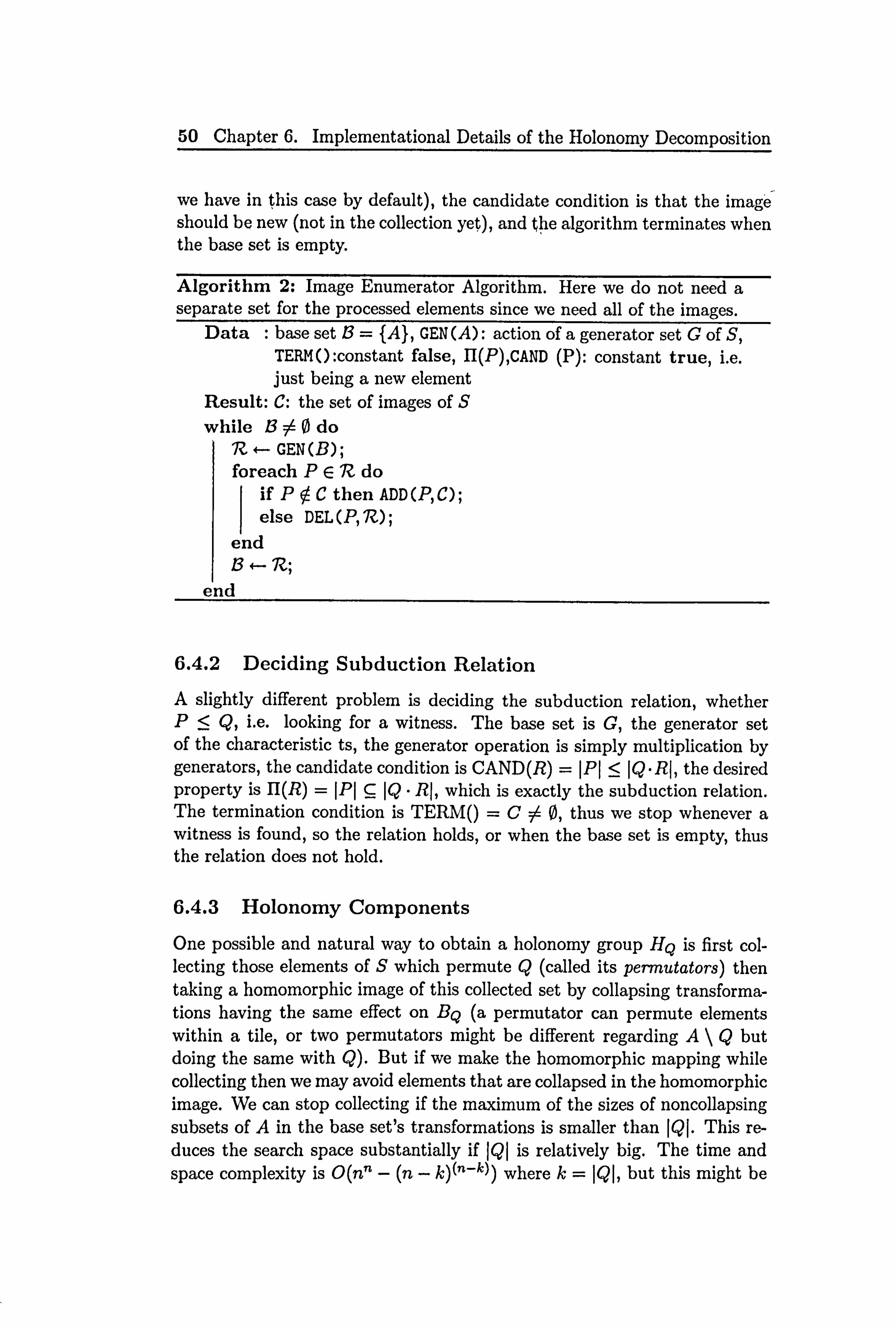
50 Chapter 6. Implementational Details of the_Holonomy Decomposition
we have in this case by default), the candidate condition is that the image should be new (not in the collection yet), and the algorithm terminates when the base set is empty.
Algorithm 2: Image Enumerator Algorithm. Here we do not need a separate set for the processed elements since we need all of the images.
Data : base set 5= {AJ, GEN (A): action of a generator set G of S, TERMO: constant false, II(P), CAND (P): constant true, i. e. just being a new element
Result: C: the set of images of S
while B: h 0 do IZ +- GEN (B); foreach PE IZ do
if PýC then ADD (P, C); else DEL (P, IZ);
end B +--
end
6.4.2 Deciding Subduction Relation
A slightly different problem is deciding the subduction relation, whether P<Q, i. e. looking for a witness. The base set is G, the generator set of the characteristic ts, the generator operation is simply multiplication by generators, the candidate condition is CAND (R) =IP1 :51Q-R1, the desired property is H(R) = IPI 9 IQ - RI, which is exactly the subduction relation. The termination condition is TERMO =C :A0, thus we stop whenever a witness is found, so the relation holds, or when the base set is empty, thus the relation does not hold.
6.4.3 Holonorny Components
One possible and natural way to obtain a holonomy group HQ is first col- lecting those elements of S which permute Q (called its permutators) then taking a homomorphic image of this collected set by collapsing transforma- tions having the same effect on BQ (a permutator can permute elements within a tile, or two permutators might be different regarding A\Q but doing the same with Q). But if we make the homomorphic mapping while collecting then we may avoid elements that are collapsed in the homomorphic image. We can stop collecting if the maximum of the sizes of noncollapsing subsets of A in the base set's transformations is smaller than JQJ. This re- duces the search space substantially if JQJ is relatively big. The time and space complexity is 0(nn - (n - k)(n-k)) where k= JQJ, but this might be

51
Algorithm 3: Subduction Relation Algorithm Data : base set G, GEN (G: generating elements of S), TERM: C 54
0 i. e. a witness is found, H(w): w is a witness, CAND(r): IPI :5 IQ - RI
Result: C containing at least one witness A +-0;
while (C =0) and (B 0) do R +-- GEN (B); foreach rER do
if rVA then if PCQ-r then ADD (r, C); if IPI > IQ - rl then DEL(rR); ADD (r, A);
end else DEL (r, R);
end B+-R;
end
close to enumerating all elements for small k. In a special case we can also stop collecting if the symmetric group is found (once some holonomy group elements are found we can use them as a generator set and check the order of the group).
6.5 Visualization
"We must see the matter at once, at one glance, and not by a process of masoning, at least to a certain degree. "
Blaise Pascal, Pensees I/1.
Our conceptual system is firmly grounded in our spatial sensory system. Some research even say that our logical (and mathematical) thinking is deeply rooted in spatial reasoning [LNOO]. We would not like to continue here the discussion about the nature of mathematics, but we would like to emphasize the importance of good diagrams in mathematical research. For instance, the whole tiling picture can be shown on a graph, where the layout enables us to grasp the full structure, not just the pieces delivered by formulas.
Our sowftware toolkit outputs the description of the graphs to be dis-
played and the actual layout is rendered by an external package. For this purpose we use the widely known and used software package called GraphViz [EGK+03].

52 Chapter 6. Implementational Details of the Holonomy Decomposition
Algorithm 4: Holonomy Group Algorithm Data :a subset of A: Q, base set G, GEN (G: generating elements
of S), TERM: C is thesYmmetric group on BQ, II(w): w permutes BQ, CAND(r): BiggestNonCollapsingSet(r) ý! JQJ
Result: C= HQ, the holonomy group of Q
whiIe dCl 54 IBQI! ) and (B --A 0) do R +- GEN (B); foreach rER do
if rýP then if BQ -r= BQ then ADD (r, C); if BiggestNonCollapsingSet(r) < JQJ then DEL (r, R); ADD (r, P);
end else DEL(rR);
end B4-R;
end
6.6 Summary
Some decisioins about the low level details of a computational implementa- tions for Krohn-Rhodes Theory (in particular and computational semigroup theory in general) had to be made before proceeding to the more interesting computational problems. The actual chosen representations come from the programmers' common sense. The problem here in semigroup theory can be described very shortly: semigroups tend to have extremely many elements.
The collector algorithms based on the idea of a brute force search, but they suffice for some specific problems like the image generation task and the problem of deciding the subduction relation. They can be applied whenever the generator operation is not redundant and the termination condition is "quick", in the sense that the probability of terminating in the beginning of the search is quite high. One might ask for the exact time and space complexity of these algorithms, but these exponential algorithms are likely to be replaced by more efficient algorithms when our knowledge about these decompositions advance.
But the brute force algorithm is not sufficient for the initial explo- ration decompositions in the case of constructing the holonomy components. Therefore the whole next chapter is devoted to this problem.
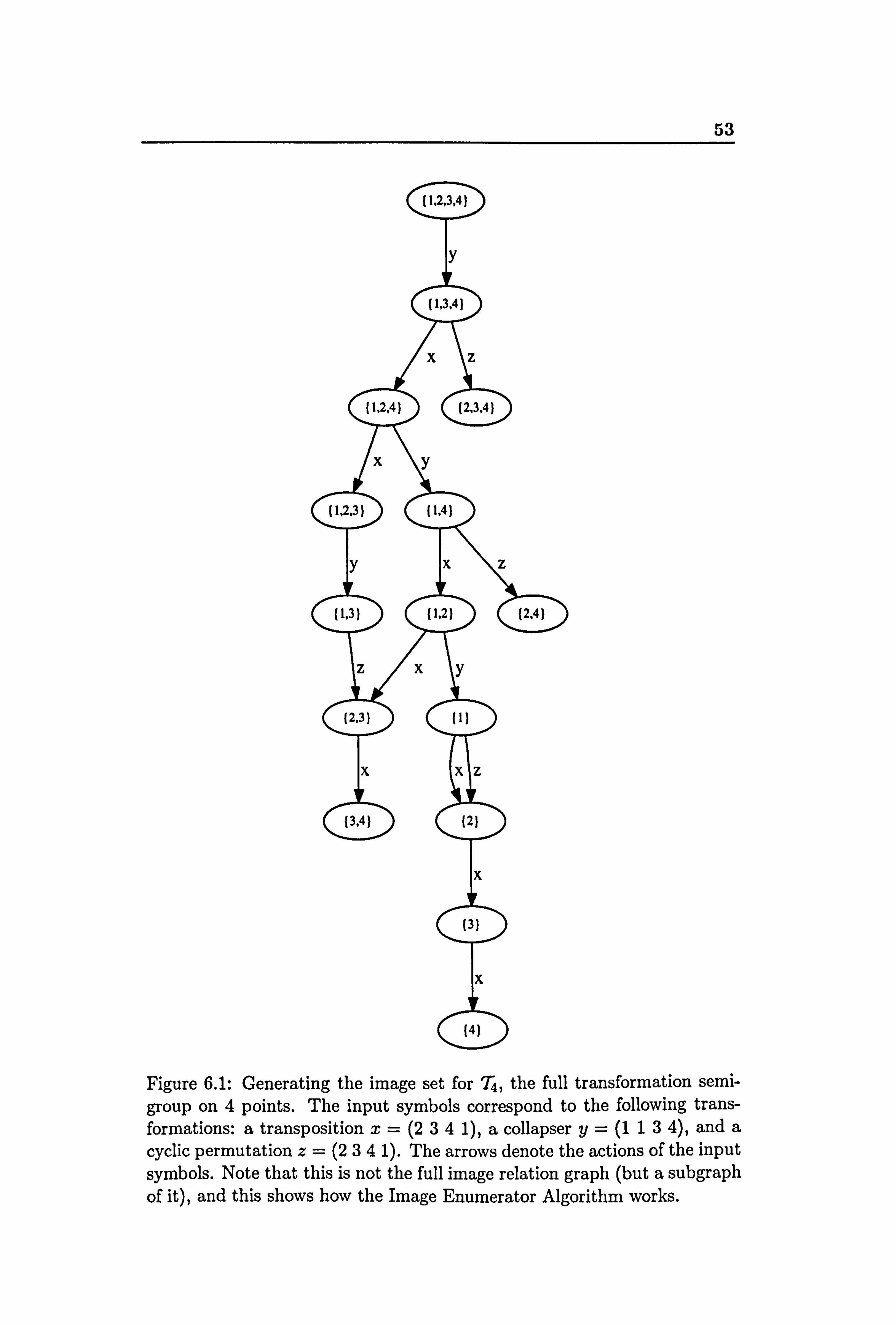
53
Figure 6.1: Generating the image set for T4, the full transformation semi- group on 4 points. The input symbols correspond to the following trans- formations: a transposition x= (2 34 1), a collapser y= (1 13 4), and a cyclic permutation z= (2 34 1). The arrows denote the actions of the input symbols. Note that this is not the full image relation graph (but a subgraph of it), and this shows how the Image Enumerator Algorithm works.
Chapter 7
Constructing Holonomy Components
When constructing the holonomy components we need to find certain sub- groups (or generators of subgroups) of the characteristic semigroup. This also can be done by using the collector algorithms, but since transformation semigroups can have so many elements we immediately bump into complex- ity issues. Some tricks can be used (for instance recognizing the generator set of the symmetric groups), but this problem demands a more systematic solution. Here we propose two methods that provide improved solutions. First we define the problem precisely, then show two different solutions.
7.1 The Problem
Let (A, S) be the corresponding ts of a given an automaton A= (A, X, 6), and let Q be an arbitrary nonsingleton element of 1, which is a subset of the state set A. Then, we would like to construct the permutation group (Q, GQ) induced by the elements of SI, where GQ is a maximal permutation group on Q, i. e. no subgroup of S, contains GQ properly, when it is restricted to Q. We call GQ the permutator group of Q. Moreover, it is also a question to decide whether GQ is trivial or not.
The ultimate goal is to have HQ, the holonomy group of Q, which is a subset of GQ, the set of transformations that permute BQ.
Obviously, the task of finding HQ can be accomplished in every case due to the finitenbss of the automaton. We only need the characteristic semigroup for checking for its elements systematically whether they permute Q or not. But this method is not satisfactory for two reasons:
Computational efficiency. The characteristic semigroup can be big even for simple automata (in the worst case n' for T,, ), therefore the enu- meration of all elements is not a usable approach for a computational
54
55
method. Different techniques (checking the size of images, stopping when a symmetric group is found) can be applied in order to reduce the search space to some extent.
Lack of a small generator set for H. Due to the advanced group theo- retical algorithms [Ser03] it is enough to have a small set of generators of a group instead of the explicit set of all group elements, but the enumeration method gives the full permutation group.
In sum, the main fault of the enumeration method is that it is a "blind" search rather than a direct way of constructing HQ. In the following we describe a method using words on the alphabet of the generating input sym- bols, which overcomes the shortcomings of the plain enumerative method.
7.1.1 Examples
The difference between HQ and GQ
Example 7.1 Let pi = (2 3 15 6 4) and P2 = (4 56 12 3) be permutations of the set Q= 11,2,3,4,5,6}, and BQ = ill, 2,3}, 14,5,6}} a tiling of Q.
Clearly both p, and P2 are nontrivial permutations of Q, but acting on BQ
P2 gives the identity permutation in HQ. Those permutations in GQ, which move elements inside the tiles only, they fall into the identity of HQ by the surjective homomorphism from GQ to HQ.
7.2 Word Based Construction Method
Intuitively permutations are connected to cycles in the state transition graph, so in order to identify permutation subgroups of the characteristic we need to check cycles of automata. This intuitive idea is more or less right, but loosely speaking, not every cycle corresponds to a permutation group el- ement. Therefore we have to clarify the notions of different cycles: the graphical cycle, which looks like and may be a permutation, and the alge- braic cycle which really is a permutation. The distinction is made by some properties of the labelling word.
Based on these notions we give simple classification of automata and show that the construction of the holonomy components can be done by
examining the cycle structure of certain derived automata.
7.2.1 Cycles in Automata
Definition 7.2 A graphical cycle in an automaton (A, X, S) is a cycle in its state transition digraph together with a word WE X+, i. e. a sequence of states al, ... a,, n>2, where the states in the sequence are pairwise

56 Chapter 7. Constructing Holonomy Components
distinct except a, = an, and w= xi ... Xn-1, -Tj EX such that ai - xi = ai+l foralll <i< n-1. The wordw=xl ... xn-l is called the label of the cycle.
Since n>2a loop edge is not a graphical cycle, and also, since ai : 34 ai+l within a graphical cycle, loop edges are not allowed.
Definition 7.3 An algebraic cycle in an automaton A= (A, X, b) is a permutation group (jai,
..., an}, (w)) for which ai = aj =ý- i=j, n>1, and w is a word in X+ such that ai -w= ai+l for all 1 <- i<n, and an -w= al.
The word w generates a cyclic group which acts faithfully on jai,..., anj by permutations. (Of course ýw) might not act by permutations on A. ) Obviously wn is the identity element. Moreover, n being greater than 1 excludes trivial one-element groups. Note that loops are not generally al- gebraic cycles. The generator of the algebraic cycle is w, and its label is
n w
7.2.2 Graphically Cycle-Free Automata
Definition 7.4 An automaton is graphically cycle-free if it does not have any graphical cycle.
The very simple structure of graphically cycle-free automata is reflected in their subduction pictures in the following way:
Lemma 7.5 (A, S) is graphically cycle-free iff on every height level in each subduction relation equivalence class there is only one element.
Proof., Let P, QEI and P =- Q but P0Q. Since P, Q are finite IPI = JQJ. Clearly by finiteness there is at least one xEQ such that xVPnQ, otherwise P, Q would be the same. Due to the equivalence of P and Q we have s, tES bijective mappings such that P=Q-s and Q=P-t and thus (st)n is the identity on Q for some n>0, by the finiteness of P, Q. Since x-s= x' : ýt x while X. (st)n = X, there must be a graphical cycle.
Conversely, a graphical cycle ensures the existence of an equivalence class with at least two elements at height zero. 0
Another way to think about the proof of this lemma is to recognize that for the singleton subsets of the state set (at height zero) the equivalence classes are exactly the strongly connected components of the automaton's state transition graph.
This result can be exploited in the decomposition algorithm since if the equivalence classes are detected to all be singleton classes, then there is no need to look for holonomy groups at all and the holonomy identity-reset ts's can be built immediately.
57
7.2.3 Algebraically Cycle-Free Automata
It is a well-known result of algebraic automata theory that the star-free rational languages are recognized by exactly those automata whose charac- teristic monoid is aperiodic (having no nontrivial subgroup) [Sch651. It is also known that deciding aperiodicity for a finite automaton is PSPACE- complete [CH91]. We are interested in this problem for certain derived automata that arise naturally in the holonomy decomposition.
Intuitively one might expect that the state transition graph of an ape- riodic automaton contains no cycles at all, but this is not true in general: there might be graphical cycles in it, while remaining aperiodic (see Fig 7.1). But with another type of cycles the notion of aperiodicity can be expressed.
Deflnition 7.6 An automaton A= (A, X, 6) is algebraically cycle-free if it does not have any algebruic cycle.
The property of algebraic cycle-freeness is tied up with the primitivity of words, which act on some states as the identity.
Lemma 7.7 An automaton A= (A, X, 6) is algebraically cycle-free iff for
all states aEA and for all words wE X+ such that a-w=a, one of the following statements holds.
1. w is pTimitive.
2. w is not primitive but has primitive root uE X+, i. e. w= ul, and au =a.
Proof: If w is primitive, then we are done. Otherwise w= u' where u is primitive. Let's suppose indirectly that a-u :Aa. Let k be the least integer that a. Uk =a (1 <k< n). Then ({a, a. U,..., a. Uk-l}, (u)) is a cyclic permutation group (with at least two elements), therefore we have an algebraic cycle, contradicting our aýsumptions.
The converse is obvious due to the fact that a trivial permutation group does not constitute an algebraic cycle, and the conditions 1-2 allow only trivial permutation groups. 0
Remark 7.8 Obviously Lemma 7.7 holds even if a-z 54 a for some left factor z of w.
It is clear that in the absence of graphical cycles there cannot be any algebraic cycle. Thus,
Proposition 7.9 If an automaton is graphically cycle-free then it is alge- braically cycle-free.

58 Chapter 7. Constructing Holonomy Components
xx
Yccýýý> YCID, ýýýx Ax 13 y
Figure 7.1: Automaton A has an algebraic cycle Q 1,2}, (a)). Automaton S has graphical cycles ab, ba, but they are labeled with primitive words.
Now we show that aperiodic automata are exactly the algebraically (not the graphically) cycle-free ones.
Theorem 7.10 The following are equivalent for an automaton A= (A, X, J) with corresponding transformation semigroup (A, S):
1. A is algebraically cycle-free.
2. S is aperiodic.
3. Holonomy groups are trivial for (A, S).
Proof. - (1) =: ý (2): Suppose S is not aperiodic, then we have a cyclic group (v) in S of order n>2, where vE X+ is a word representing the generator. Thus Vn is the identity of the cyclic group, V= Vn+1 and v0 V2. Therefore 3asuchthat a-v 54 a. V2 and a-v = a. vn+l. Let a' = a-v, thus a'. Vn = a/ and since A is algebraically cycle-free we can apply Lemma 7.7: let u=ý, fv_n_ = ý, Fv, then we have a'. u=a, a'. v= a' and finally a. V2 =a-v, which is a contradiction.
(2) =: ý- (1): For the converse we use again an indirect proof: Suppose there is an algebraic cycle, i. e. Qaj,...
' anI, M) is a permutation group with ai E A, WE X+ and n>1. Therefore Z, the cyclic group with n elementsl divides S. This cannot happen when S is aperiodic.
(2) . 4-* (3): The components of the holonomy decomposition are all divi-
sors of the original semigroup, thus aperiodic semigroups have only trivial holonomy groups, and wreath products and divisors of aperiodic transfor- mation sernigroups are aperiodic. 0
Corollary 7.11 An automaton A= (A, X, 6) is aperiodic if and only if
Va E A, wE X+, x-w=a =* a- --, 1-w- = a.
The distinction between algebraically cycle-free aperiodic and nonape- riodic automata is rather subtle. Two automata having the same state- transition graphs regarding their connectivity might belong to different classes depending on how the input symbols act on the state set (Fig. 7.1).

59
Figure 7.2: An automaton 4 with state set A= 11,2,3,4,5,6} and alphabet Ix, y}, where x and y are transformations with x= (3 4134 3), y (436642).
7.2.4 Non-Aperiodic Automata
A main concern of the holonomy decomposition is to find the nontrivial holonomy groups. Fortunately the tiling picture provides tools for locating the elements of IT for which there exist nontrivial holonomy groups.
Lemma 7.12 For an element Q of -7 in the tiling picture of (A, S) if there is a nontrivial holonomy group HQ, then in its set of tiles BQ there are at least two distinct tiles tl 9 t2 such that tj --: t2 -
Proof. HQ being nontrivial means that there are some pair(s) of tiles for which there are transformations permuting them and thus they are mutually subduction related. 0
The converse is not generally true as we can see in the example of an automaton (Fig 7.2) with tiling picture (Fig 7.3). For a trivial HQ the set of tiles BQ may contain distinct equivalent tiles, see Fig 7.4. In order to determine whether we have a nontrivial holonomy group for aQEI we define an extended automaton and examine its cycle structure. Denote the equivalence classes of subduction relation by El to EN.
Lemma 7.13 If PE Ej and for some sES, P-s=Q such that QV Ej (leaving the equivalence class) then there is no transformation tES such that Q-tE Ei (no way back to the original equivalence class).
Proof., Suppose there is such at that Q=P-s and P' =Q-t with P -= P'. Due to the equivalence we have P= P' - s" for some s" E S, therefore Q- (ts") = P'. s" = P, thus Q =- P, which contradicts the original assumption that we leave the equivalence class of P. 0

60 Chapter 7. Comstructing Holonoiny Components
Figure 7.3: The tiling picture of automaton A in Fig. 7.2. The equivalence chv, scs are denoted hy boxes. Equivalence classes with clements haviin, 11oldrivial holollonly orollps arc shaded. Arrows ending in phips denote the tile of' relation.
IAI Is (KHm, EQ im the Moll (A equiwdence chLsses which contain at least
mw I He of QC1. Formally: E(ý =UI,,,, nl?, ý, qEj. Then the Nlc (rutoinalmi
of Q is AM& as AQ = (F, (, ) u Jý I. X. -ý), where , is a sink state. the inpi it
alphabet X is the saille, (IS the original allionlat-oll's, and -,, is the 11,11111-al extens, ion of' 6 to act oil subsets of A providing that if the image is not ill
some E, then it is, ý. This way ý represents going to another equivaleiwe class not contained in EQ, but accor(ling to Leluma, 113 this cmi be n1wesuilted ws a sink since there is no Nva ack. y to come 1),
The equivalence classes ill EQ forin strongly connected components ill AQ. When (Icteriniiiing the nontriviality ofII(2 we look for algchraic ill these components. NVe look not simply for independent algebraic cycles hi each (imnponent as a mwd of a c. vde ndght not p(Tinim v the t& clunicilts ill another component. but for parallel algebraic cycles'. This way we can reca. st the characterization of a, holonmny group element in terms ofalgebraic cycles. More Forillall. v:
Proposition 7.14 H(ý cýrIsfs a word it, c A+ and B(., ) coll bc 1)(11-11"how'd IlIto ITI
.... 17'k I sti bscts sitch, that cithcr
1. Tj consists of exactly onc tile and Ti - u) = Ti, or

I
x
Figure 7.4: Two tilc it it I oinahi ofautoniatmi A it i Fig. 7.2. A is trivia I, while AJ2,3,61 With g('11""'to" Y-
ý2. Tj - (w) c B(ý nE'j for sonic 1<j< Ar. wid, (Tj - ýw), ýtv)) is wn algcbruic cyclc in A(ý)
holds for all Ti, I<i<k, aml (2) must hold, for (it Icast onc Ti.
In short the proposition characterize's whell the t ralisforillat ion induced I)Ný Ill liontrivially permutes B(). This transformation i", clearly a 110111rivial hololl-
only group element. From Leinina 7.13, Ti - u, " c (13(ý nE j) Follow", for ally i) ýý 0. Tfierefore the algebraic cycles, contained ill B(ý generated 1)
,, 11" are '111 dis or loi of t 1(, i
, joint. If ail intersections, (B(ý) n Ej) are singleton-s, I le 1 11
contaill's all algebraic c. Vc1c then H(ý is trivial. This fact can be ew1oited ill efficielit decompo,, ition algorithins of the ImMumi
*v Awonumshion Is, vx-
chiding cases where the collstructioll of the 1101011011ly ý1111. ollp Should not be
atIvnilMd. We describe all algorithill for constructing the maximal groul) 1wrinut-
ing ail arbitrary given subset, of a fillite state alitoillatoll iii(Iliced bY the

62 Chapter 7. Constructing Holonomy Components
input symbols, and characterize its computational complexity. This prob- lem naturally arises in the computational implementation of the holonomy decomposition for the Krohn-Rhodes Theory.
7.2.5 The Algorithm
We described the problem on two different levels: finding permutators and finding the holonomy group elements. In order to avoid the notational bur- den we present the solution for the permutator problem. It is easy to trans- late into the holonomy group problem (but not the opposite direction). Once we know (Q, H) then (BQ, HQ) is obtained by making (BQ, H) be faithful, as in Example 7.1.
This algorithm is yet another example of collector algorithms, so the idea is simple again. We generate words and collect hose that induce per- mutations on Q. But the details are a bit more complicated.
Generator Operation
We can just generate words starting from the empty word and applying input symbols systematcially. But we know something about the form of the possible candidate words. Since the words labeling transformations in GQ should permute Q, the corresponding paths start from and end in Q. So we define the following sets of input symbols:
Qout : -- Ix EXI 3a E Q, b EA such that a-x= b}
Qin=IxEX13aEQ, bEA suchthatb. x=al Note that the names might be a bit misleading, since an incoming edge might come from Q itself, and the outgoing might stay in Q. In the next section it will become clear why we choose these names.
The generation of words has three stages:
1. Single letter words in Qi. n Q,, u,. 2. Two letter words in Qin X Qaut-
3. Words in the form xiwx,,, where xi E Qin) Xo E Qouti WE X* gener- ated systematically in alphabetical order.
This way we do not need to check words that clearly cannot permute
Candidate Property
We know that the paths corresponding to the permutations of Q start and end in Q. But how freely can they go around meanwhile? We can go "as far" as we like until we can come back eventually, which - in terms of the

63
state transition graph - means that we cannot leave the strongly connected components. The orbit of one particular point a should stay within the strongly connected components of a denoted by Ca. CQ " UaEQ Cal is the union of strongly connected components of the states in Q. Finding the strongly connected components of a digraph (here of a state transition graph ) can be done in linear time by acyclic ordering (topological sorting) of vertices using depth-first search [BJG02].
A word w represents a permutation of Q if Q-w=Q. Once a word w is found to be a permutation, we can stop extending it. This can be shown by a simple argument: w is minimal in the sense that no proper left factor of it is a permutation. Suppose wv is the next permutation in the continuation of w (no proper left factor is a permutation, except w). Then, either w=v, or v itself is a permutation. In the first case we clearly do not loose anything by stooping at w. The same is true for the second case, since if v is different then it is found independently as another branch of the search-tree.
A particular permutation (and transformations in general) can be ex- pressed by many different words. We do not need to keep track of all those words but one. Therefore we define an equivalence relation on words by:
w=-Qviffa-w=a-v VaECQj
and it is enough to deal only with the equivalence classes X+1 =-Q of words. A class is represented by one of its elements, namely the first word found by the breadth-first search. Obviously, we can safely ignore what permutations do on A\ CQ.
In sum, for each newly generated word w we check whether the following properties are valid:
a word equivalent (realizing the same transformation when restricted to CQ) to w is already processed,
*w is a permutation of Q (this is the desired property),
*a-wý Ca for any a r= Q (leaves the strongly connected component),
* IQ - wl < IQI (some states in Q are collapsed). If any of these conditions is true, then we stop extending w. Otherwise, if none of the above conditions are satisfied then we continue extending w. Clearly, the generations terminates, since we collect the transformations (not the possibly infinitely many word representations of them) and they are finitely many.
7.2.6 Examples
and Q,,.,, t Consider Figure 7.4 again. B{1,3,4} is {11,31, {1,41, {3,4}}. {1,3,41j, = {xJ, {1,3,4},,, t = {x, y}. In the first case we have some seaxch space reduc-

64 Chapter 7. Constructing Holonomy Components
tion, while in the case of outgoing edges we gain nothing as the set of input symbols is exactly Ix, y}.
B(2,3,6) is j{2,3}, j2,6}, j3,6}}. 12,3,6}i,, = jy}, {2,3,6},, t = Ix, y}. In the first case again there is some search space reduction. And the very first step in the generation of words finds a generator: 12,3,6}i,, n {2,3,6} ... t 1Y}-
The Good and the Bad
Again, we would like to use the full transformation sernigroup for testing our method. The main concern now is the number of generators provided by the algorithm. Recall that in the decomposition of the full ts we have sym- metric groups (plus constant maps) on all levels. Therefore the components can be generated only by two permutations, a cycle and a transposition. Decomposing T6 gives the following number of generators:
Level #Generators Order of holonomy group 1 2 2 2 6 6 3 24 24 4 40 120 5 2 720
Boldface numbers indicate cases where the generator set equals the gener- ated group. On the top level it is the minimal number of generating elements and this efficiency is due to the fact it is 'easy to fall down from the peak', i. e. there are not many elements in the equivalence class to wander around. But when the tiling picture gets wider the algorithm becomes very inefficient: it enumerates all elements of the generated group.
Curious readers might want to check the output of the algorithm on the fourth level. It is a challenging exercise to track down the generator words (listed on Fig. 7.6) on Fig. 7.5.
7.3 Dependency Function Based
The real machinery of the cascaded automaton hides in the dependency functions. We tried to emphasize this insight before and now we present something more convincing: a method for constructing holonomy compo- nents by using the values (component actions) of the dependency functions. We use the algorithm for lifting the transformations for finding the holonomy group generators.
The idea is simple and comes from the following origins:

65
Figure 7.5: The tile autonlaton of of the fourtl) level's Component of the I Io](), MIlly decomposition of T,. ne generators are: I, = (2 :3456 1),
y- (I 13 .45(; ), ý- = (2 1 :345 6).

66 Chapter 7. Constructing Holonomy Components
Word in GQ in HQ z (2 13456) (423 15) xyxxxx (512345) (45 123) xxxxxx (123456) (12345) xzxxzxx (5 12436) (43 1 25) xzxxxzx (5 13246) (4532 1) xxxzxxx (123546) (15342) xxxxzxx (124356) (12543) xyxzxxx (4 12354) (42 153) xxxxxzx (132456) (32 145) xyxzxxzx (4 13254) (4235 1) xyxzxzxx (3 12453) (42 135) xxxzxxzx (132546) (35 142) xxxxzxzx (134256) (3254 1) xxzxxxxx (2345 16) (345 12) xzxxzxzx (5 13426) (4 1325) xxxzxzxx (124536) (13542) xxxzxzxzx (134526) (3 1542) xxzxxxxzx (3245 16) (14532) xxzxxzxxx (2354 16) (342 15) xxzxxxzxx (2435 16) (543 12) xxzxxzxzxx (2453 16) (542 13) xxzxxzxxzx (325416) (14235) xxzxxxzxzx (3425 16) (54132) xxzxzxxxxx (345 126) (5 1234) xxzxzxxzxxx (354126) (2 1534) xxzxxzxzxzx (3452 16) (5423 1) xxzxzxxxzxx (435126) (3 1254) xxzxzxxxxzx (245 136) (532 14) xxzxzxzxxxxx (451236) (2345 1) xxzxzxxzxzxx (453 126) (2 1354) xxzxzxxxzxzx (425 136) (13254) xxzxzxxzxxzx (254 136) (2 35 14) xxzxzxzxxxxzx (45 1326) (2 1453) xxzxzxzxxxzxx (35 1246) (2543 1) xxzxzxzxxzxxx (541236) (5342 1) xxzxzxxzxzxzx (452136) (23154) xxzxzxzxxzxxzx (54 1326) (5 1423) xxzxzxzxxzxzxx (53 1246) (3 542 1) xxzxzxzxxxzxzx (2 5 1346) (254 13) xxzxzxzxxzxzxzx (52 1346) (15423)
Figure 7.6: The generator words for S5 in the decomposition of T6 produced by the word based construction method.

67
Lifting generators only. For lifting the transformation semigroup to the wreath product semigroup it is enough to map the generators only (see division in Section 2.1.5). This implies that the dependency functions of the generators contain all information about the generators of the holonomy components, thus they encode the whole wreath product ts.
Holonomy permutations are moves within equivalence classes. With the help of 'M-p and 'mp we can move between an arbitrary element and the representative of a subduction equivalence class. By con- catenating these maps we can move from any element to any other element within the equivalence class. Thus having certain set of these maps might draw the generator set for holonomy components, since a holonorny permutation is built up from synchronized movements in some equivalence classes, as showed in Section 7.2.4.
'Cheating' gives component actions. For lifting the original ts in the mathematical proof of the Holonomy Decomposition Theorem (Section 5.6.1) we do some kind of cheating: we do not give the lift in its full detail (in a small set of formulas or as a lookup table serving the needs of a practical minded computer scientist), we just describe a method for mimicking the lifted transformation in a particular situation (i. e. a given cascaded state), for giving the component actions by combining Mp and 'Mp maps. By knowing the original transformation we tell for a particular cascaded state what the transformation lift would do in a particular situation, which are exactly the component actions.
7.3.1 The Algorithm
Since we cannot give a nice formula for the dependency functions, we han- dle these functions as lookup tables. The tables map upper fragments (Bi,
..., Bh), 1<i<h of cascaded states, the elements in B, x ... X Bh to holonomy actions (constants and permutations). To make these functions fully defined for those upper fragments not appearing in the lookup table we define their values to be the identity map. The steps for getting the holonomy generators are the following:
1. Generating A(A), i. e. enumerating all tile chains. Cleaxly, in terms of efficiency this is the weakest part of the algorithm, since there can be
many tile chains. For the time being we do not know what subset of the tile chains is needed for defining the dependencies.
2. Applying each generator lift to A(A) by using the method for lifting the transformations described in Section 5.6.1. Whenever we get a nontrivial holonomy group action we record the arguments of the de-
pendency function and its value. A nontrivial action is a constant map or a permutation which does not act as an identity on the tiles.

68 Chapter 7. Constructing Holonomy Components
3
2
I
0
Figure 7.7: Tiling picture of the elevator automaton with 4 states.
3. For each recorded permutation we have to decide exactly which com- ponent it belongs to, if there axe parallel components on a level. This is done by the the successive approximation (see Section 5.5.1) of the upper fragments. The equivalence class of the resulting set indicates the right component.
After drawing the lookup table, the sets of permutations for each com- ponent will be the corresponding generator sets. If there is no entry or there are only constant map entries, then that component's holonomy group is trivial.
7.3.2 Example
An Aperiodic Example: the Elevator Again
Recall Example 4.2. Now we are interested in the dependency functions of the lifts of the generator transformations. To keep it simple we consider the elevator with 3 levels. The generators are d= (1 12 3) and u= (2 34 4). The skeleton can be seen on Fig. 7.7. The algorithm gives the following lookup tables (using the notation of lookup tables in Example 2.2):

69
(1,2,3,41 ýý -)
3( (1,2,3,4) )3
(1,2,3} 2)2( (1,2,3) ))2
(2,3) (3,4) )I( (1,21 )4--*( 12,3) )I
0 ý)I 0
Figure 7.8: State lifts of states 3 (left) and 2 (right) in the holonomy decom- position of the elevator automaton with 4 levels. The bidirectional arrows denote the coding and encoding of tile chains.
; a:
f3uO constantf2,3,4} f2u({2,3,4}) constant{3,4}
flu({3,4}, {2,3,4}) constant{4}
d:
fd 3"() = constant{1,2,31
f2d({1,2,3}) = constant{2,3} f1d(J2,3}, J1,2,3}) = constant{3}
Note that the indices of the functions correspond to height numbers, fi gives an action on the ith level.
It is somewhat surprising that there axe only few entries in the lookup table: only 3 entries per transformations, while there are 8 (23 tile chains) states in the cascaded product. But still, the mappings within the equiv- alence classes and the successive approximation do the job. Let's consider the following cascaded state: a= ({4}, 13,4}, 11,2,3}), which is a lift of 3. Let's apply jto this cascaded state. We know that it should produce a state lift for 2, otherwise the division would not hold. For the the top level (third) we have a constant map defined, so we get {1,2,3}. On the next (second) level dis defined for the fragment (, 11,2,3}), so we apply the constant map yielding {2,3}. On the bottom level (first) we have no en- try in the dependency function lookup table, therefore we leave the existing
ý10

70 Chapter 7. Constructing Holonomy Components
component there. We got a-d= (141,12,31, {1,2,3}), and that is a lift for 2, as expected (check Fig. 7.8).
Dependency Functions for a Nontrivial Holonomy Group
Recall Eilenberg's example again (Fig. 5.3). We have a nontrivial group for the tiles B13,4,5}. Actually it is S3. Here are the corresponding dependency function entries:
5ý: fl'({l, 2,3}, 11,2,3,4}) = (3 4534 4)
y fl' (11,2,3}, 11,2,3,4}) = (3 5435 3)
The tiles axe singleton sets 131,14} and 15}, therefore it is easy to check that one function value is a cyclic permutation, the other one is a transposition. Together they form a minimal generator set for the symmetric group.,
In general, the minimality of the generator set is not guaranteed, since we may have to different generators for the original sernigroup which act the same way on a subset of the state set.
Narrowing the Skeleton
Observing that since we have a bijection between tile chains and cascaded states and we know the mapping between them (see Section 5.4.2) leads to the idea that we do not need the full skeleton in order to construct the holonomy components. We need only the tilings of the representatives, and tile chains can be recovered from them, if needed. How much percent is this part compared to the size of the full skeleton? Here is a table about the ratio in the case of full transformation sernigroups (also see Fig. 7.9).
Semigroup Ratio _ S2 100%
S3 85% S4 80% S5 58%
L S6 39%
This seems to be a very good news, since as I gets bigger the ratio of the needed subsets versus the size of I decreases. The bad news is that we cannot exploit this property unless we solve the problem of generating tiles locally (see the problem of nonimage tiles in Section 5.7.3).

71
Figure 7.9: The partial tiling picture of T-,. Only the equivdence class representntive-, and dicir tiles are displayed. Tlw'ýc an, liceded fOr carrying Out transfOrnintion", ill the wreath producl scillit"'roup. I'lle other clements of I Can he -ellerated hy Inapplit", c'I'scaded shites to tile chain: -i.
7.4 Summary
Construct im, the 11010110111v compollent is a critical lsý,, Ile ill 1111plellwilt illo tile holonoillY decomposition. Here described two difl'Crcut inethods. The first one is it inore advnilced ""cal-ch thall the brilte-force appro(Ich. It
uses, the knowledge about Ihe structure of tiling and its, relations to the
equivalence classes. Exploring these connections improved om- undenstand- iil, ). of liololloill decolilpositiou. However, regni-ding its efficiency ill terms
of a sinall generator set, it is still not satisfývino-. Therefore we pi-csented phip the depen- another approach ill a completely different maimer. Leveratl
el dency flinct loll", we pet a gencrator set, comparable ill size to the origilml n t, autollint oil's generator set.
Chapter 8
Applications
"The engine turns, the Maker rests. " Imre Madach, The Tragedy of Man, 1860.
The hierarchical decomposition of automata gives us wonderful promises regarding its applicability: automated object-oriented programming in soft- ware development [Neh94], formal methods for understanding in artificial intelligence [Neh96a]. The least number of needed levels for decomposition provides a widely applicable integer-valued complexity measure, including applications ranging from electrical engineering and physics to evolutionary biology [Rho7l, NROO, Neh96a, Arb68], just to briefly mention some im- portant keywords. We also have now working implementations, therefore it is reasonable to ask what happens to the promises. Why are the foretold revolutionary results not delivered yet? There are three basic reasons:
1. Since this work gave the first computational implementation, simply due to the lack of tools before no one has tried to do practical appli- cations before.
2. Our knowledge of the detailed inner workings of actual decompositions is still rudimentary.
3. The implementations are not yet scalable.
Our assumption is that the second reason is due to the first one. Therefore we think that by studying small but nontrivial examples, understanding otherwise well-known structures differently, via hierarchical decomposition, eventually will lead us to scalable implementations by exploiting the special properties of the decompositions.
Here we take this route, first we will show some features of the holonomy decomposition emphasizing the role of the subduction equivalence classes using spatial clues. Then we decompose finite residue class rings modulo n represented as semigroups. And finally we discuss the difficulties of applying hierarchical decompositions as formal models of understanding.
72

73
8.1 Understanding the Holonomy Decomposition
The holonomy decomposition gives us a hierarchically structured finite au- tomaton, but it is not immediate how this cascaded automaton works, and how it is related to the original automaton although a division is constructed in the proof of Theorem 5.1. Therefore it is worth examining illustrative ex- amples in order to understand how in detail the holonomy decomposition provides hierarchical coordinate systems on finite automata. Since we are human beings living in a three-dimensional physical world, it is easier for us to comprehend abstract constructs in spatial terms. Here we will first consider state transition diagrams with some specific forms. The nodes rep- resent points in space and the edges represent the connections in that space, thus input symbols correspond to movements in the space.
8.1.1 Decompositions Without any Hierarchical Dependence
The most basic examples are with only one hierarchical level. These are the automata whose characteristic sernigroups are groups (possibly with constants). As all input symbols are permutations or resets I consists of the full state set and the singletons.
Torus. The torus is basically amxn grid of points with a wrap-around (Fig. 8.1.1). Since we can get back to the a state by going into one direction,
we have loops, thus we have nontrivial groups. Wherever we are, we can reach any other point, thus there is no irreversibility of the operations and this yields the very simple holonomy decomposition: the only component of the decomposition is (mn, C,,, x Cn).
r
ddrddrdd
0
r
Figure 8.1: A2x3 toroidal grid as a state transition graph of an automaton. States are denoted by the circle nodes (without names, but can be addressed by coordinates). The input symbols axe d and r, corresponding to moves on the grid: down and right.
8.1.2 The Role of Subduction Equivalence Classes
The role of equivalence subduction classes is that we do not have to consider explicitly those elements of. T which behave the same way under the action of

74 Chapter 8. Applications
S, i. e. their holonomy groups are isomorphic and there are transformations in S to establish this isomorphism.
Irreversible Mesh. Let's consider automata with transition graphs of shape of a bounded rectangular plane, and with two input symbols going left and down. Clearly, these automata are aperiodic, since applying any of the input symbols collapses states towards the left or bottom edges. More- over, each element of 11 forms a subduction equivalence class on its own. The
0dro0d '-.,,. o
dr0
rIr 0
------ ; -- 0od, r uu
dd
Figure 8.2: A2x3 irreversible mesh automaton. On the left are 3 exam- ple elements of the set of the images. The images are rectangles with the common bottom right corner. Each of them form a singleton equivalence class on its own, due to the fact that we cannot move backwards in either direction.
example on Fig 8.2 shows a2x3 mesh with input symbols r, d for moving right and down on the grid. The bottom-right corner is the state where even- tually the movement ends up, therefore this state is contained in all elements of 1 (except the other singletons), which are basically the rectangles with the
common bottom-right corner. Its decomposition is (T2 x 12) ? (T2 x 13) IT-3, III = 11.
Partially Reversible Mesh. The situation changes when we have the other directions as well (going up and right) as cycles appear. Despite the cycles in the graph it is still aperiodic (for a further discussion determining aperiodicity in automata see Section 7.2.3). But the equivalence classes are not singletons any more. They consist of all rectangles of the same dimensions.
The example of 2x3 mesh on Fig. 8.3 shows the automaton and one T particular equivalence class. Its decomposition is (T2 x 12) z (T2- -x14) z 4,
I-11 = 18. Although there are more elements in -T than in the previous irreversible case, the decomposition is quite similar, since the equivalence classes are not singletons.

75
U'l u u, r II
000 31
Fo Foý Foý rr
ududu II ED 1-0ý Fo- d()-
--"( )
57 000
rr
d, l d d, r
10 o000
10 o000
10 0- C)
10 0 01 000
000
000
Figure 8.3: A2x3 partially reversible automaton with all its equivalence classes. An equivalence class has elements that are rectangles with the same dimension.
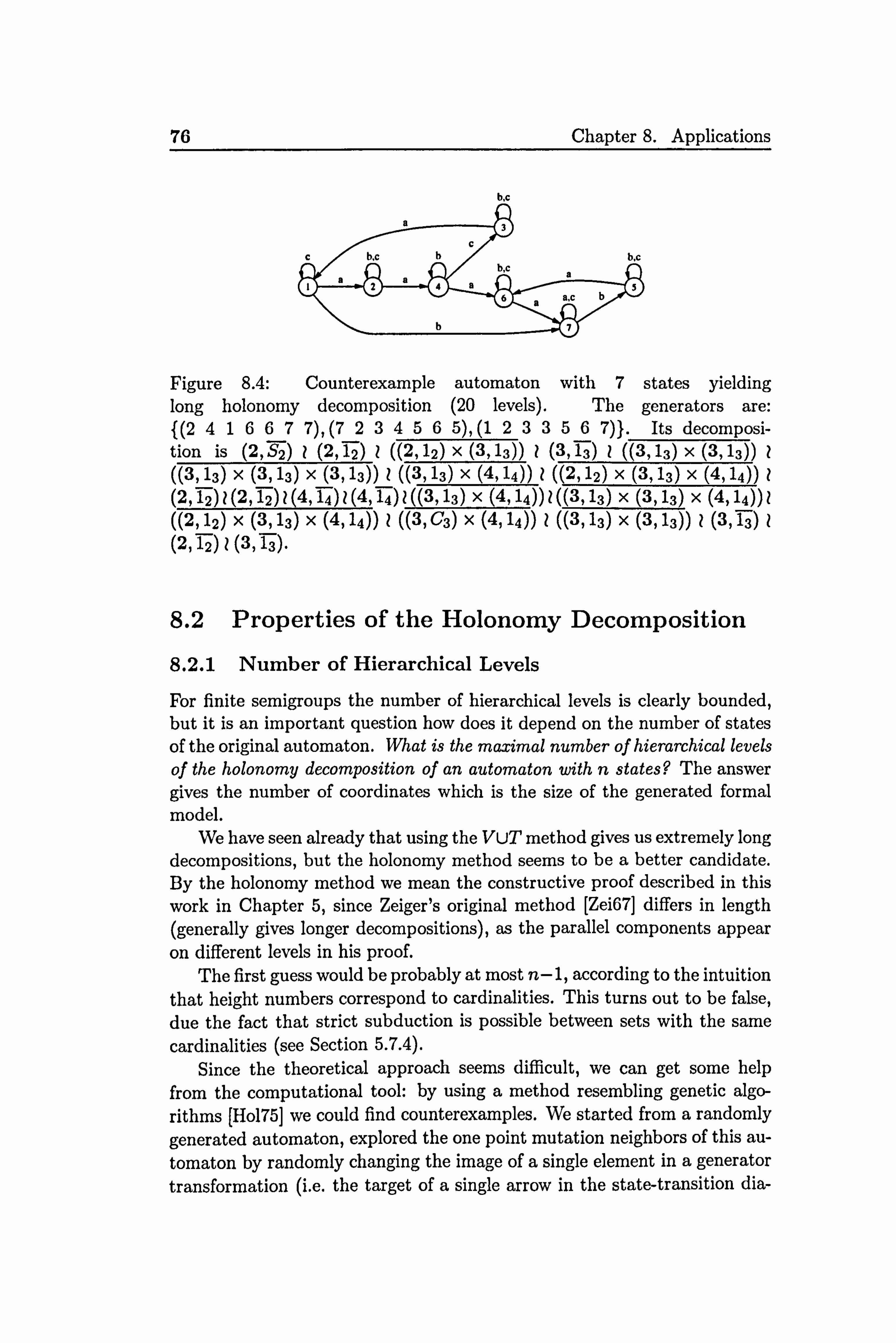
76 Chapter 8. Applications
b, c
Figure 8.4: Counterexample automaton with 7 states yielding long holonomy decomposition (20 levels). The generators are: 1(2 41667 7), (7 23456 5), (1 23356 7)}. Its decomposi- tion is (2, Y2) I (2, T2) 1 ((2,12) x (3,1-3)) 1 (3, T3-) 1 ((3,13) x (3,13)) ((3,13) x (3,13) x (3,13)) 1 ((3,13) X (4,14)) 1 ((2,12) x (3,13) x (4,14)) (2, T2)1(2, -12-)1(4,14-)1(4, T4-)I((3,13) x (4, T4))I((3,13) x (3,13) x (4,14M ((2,12) x (3,13) X (4,14)) 1 ((3, C3) x (4,14)) 1 ((3,13) x (3,13)) Z (3,1-3) 1 (2, T2) 1(3,1-3).
8.2 Properties of the Holonomy Decomposition
8.2.1 Number of Hierarchical Levels
For finite sernigroups the number of hierarchical levels is clearly bounded, but it is an important question how does it depend on the number of states of the original automaton. What is the maximal number of hierarchical levels
of the holonomy decomposition of an automaton with n states? The answer gives the number of coordinates which is the size of the generated formal model.
We have seen already that using the VUT method gives us extremely long decompositions, but the holonomy method seems to be a better candidate. By the holonomy method we mean the constructive proof described in this work in Chapter 5, since Zeiger's original method [Zei67] differs in length (generally gives longer decompositions), as the parallel components appear on different levels in his proof.
The first guess would be probably at most n-1, according to the intuition that height numbers correspond to cardinalities. This turns out to be false, due the fact that strict subduction is possible between sets with the same cardinalities (see Section 5.7.4).
Since the theoretical approach seems difficult, we can get some help from the computational tool: by using a method resembling genetic algo- rithms [Ho175] we could find counterexamples. We started from a randomly generated automaton, explored the one point mutation neighbors of this au- tomaton by randomly changing the image of a single element in a generator transformation (i. e. the target of a single arrow in the state-transition dia-

77
gram), then selected for the longest decomposition and repeated the same cycle. We found experimentally the following state set size and height num- ber pairs: (5,11), (6,15), (7,20) - see Fig. 8.4, and (8,26). Hence even 3n +1 does not bound h(A). Note that the holonomy decomposition is still more efficient than the VUT technique in terms of the length of the wreath product (see [ENN041 or Chapter 4).
We do not know an exact bound for the length of the holonomy decompo- sitions yet, but we can summarize the observations of our genetic algorithm experiments.
Observation 8.1 Long holonomy decompositions tend to have a low num- ber of nontrivial holonomy group components with small cardinality.
It seems that in order to build a high skeleton, we need sufficiently many elements in -7, and that is provided by the nontrivial group components' permutations. But on the other hand, if we have a group component with high order, then its subgroups might also be components on lower levels, thus collapsing the hierarchy.
8.2.2 Size of a Component's State Set
Another important question is How many a tiles can a set Q in I have given its cardinality? The answer gives the number of states of a component, contributing to the size of the state set of the cascaded product. Intuition might say that if we have more tiles, then they should become inclusion related, thus not satisfying the definition of being a tile, so that a subset QE -7 should not have more tiles than its caxdinality as for the full ts.
However, mistyping one character the generators of R6 (the semigroup of integers modulo 6, see Section 8.3) yielded an automated decomposition, where the top level set with cardinality 6 has 14 tiles (see Fig. 8.5). This example also shows the ruggedness of the landscape of the decompositions, since just changing one single image of a transformation results in a com- pletely different hierarchical structure and sets of tiles.
The analysis of the example in Fig. 8.5 shows that the high number of tiles for the top level component is due to the missing sets with cardinalities between the top and next level below. This suggests set theoretical consid- erations: What is the largest number of tiles that are not subsets of each other? Considerations based on examples led to the following conjecture:
Conjecture 8.2 VQ E 1, JBQJ :5 (L, ', ) where n= JQJ. 2
Actually we can show that it is indeed possible that JBQJ We U2
need the generators of the symmetric group S.,,:
(2 3 ... n-1 1), (2 13
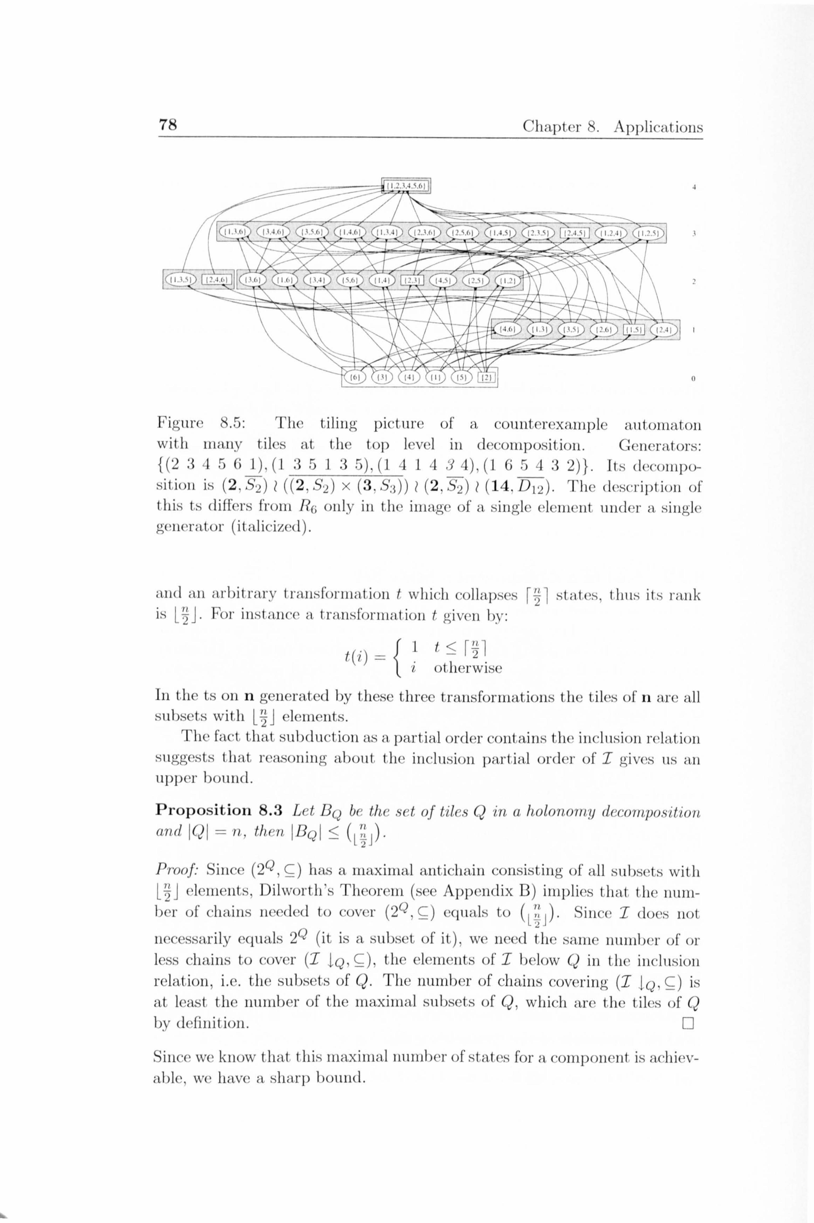
78 Chaptei-8. Applications
Fi-m-c 8.5: The tiling picture of' a Collilt(TexallI)Ic witolliatoll With 111all , N, tilcs at, the top level ill decomposition. Generators: 1 (2 3A5(; 1). (1 :1513 5). (1 -1 14Y 4), (1 (; 5 -1 :3 2) 1.1 Is deco iii po- sition is (2. S, )) ý ((2ý S2) x (3. S: j)) ? (2,,; 2) 1 (14. D12). 'I'll(, description of' thi's t.,, (Ilft, (, I. s fi-oill I? (j only Ill the lillage of a sill"de cleillent 1111der a Single (), ellerator (italicized).
and all arhitrarv trall'S101 . illation f which collapses stot ('s. I hus It's railk 2 is For instmice a transfonliatioll t gjý,, (qj
<[ 11 1
2 i ot'llel-wise
In the ts on n generated by tlll. (, (, trall"'formatioll", the tiles of' 11 are all "llb. set's With [111 clements. 2
The fact that subduction as I partial order contains the inclusion relation suggests that, rc; lsollill. " about the inclusion partial ordei- of I gives us an upper bound.
Proposition 8.3 Let B(ý bc the sct of tilcs Q in a holanamy (1ccamposdion awl Qj - i). thcti B(dj <
Proof- Since (2ýd, C) has a maximal alitichaill Consisting of all Subsets with elements. Dihvorth's Theorem (sec Appendix B) implics, that the will
bel. of chaill", liceded to cover (2Q. C) cquals, to Since I does not
necessarily equals 2(ý (it is a subset of it)ý we need the saille 1111111her of' or less chaills to cover (I fQ' C), the etenlents ofl below Q III (11c IlIcIllsioll relat ioll, ix. the subsets of Q. The number of chahus covering (I IQ, g) is
-it least the number of' the maximal subsets of Q, which are the tiles of Q by defillition. 11
Since we kiiow that this maxillial 1111111berofstates for a component is
able, we have a sharp bound.

79
8.3 Decomposition of the Rings of Integers Mod- ulo n
The transformation semigroup of finite residue class ring of integer modulo n is a set n with the operations of addition and multiplication modulo n, and is denoted by R,,,.
8.3.1 Representation
Integer modulo n residue class rings Rn can be represented by automata. The state set is n, the residue classes modulo n. The transformations corre- spond to the operations of the ring represented as one-argument functions such as +1, x2, x3 and so on. As generators, clearly we need only at most +1 and the multiplications by the prime elements smaller than n. The characteristic semigroup of this automaton is denoted by S(Rn).
Proposition 8.4 JS(Rn)1 = n2.
Proof., S(Rn) is a noncommutative semigroup, a semidirect product of the additive group Cn and the multiplicative monoid in Rn, since the elements are given by the affine linear transformations of the form xk+I which are closed under composition. It is easy see that all distinct pairs k, 1En give distinct transformations of n, therefore we have n2 transformations. 1: 1
For example, the following automaton represents the R4, the residue class ring of integers modulo 4:
x2, x3 0 +1 oc
x3 +1 +1, x2
x2 x3
13
+1 2 x3
+1 x2
Since it is easy to move between the ring and sernigroup notation, we will use the notation am +P instead of (m -x a) where mEn and a,, 3
are elements of the ring R,,.
8.3.2 The Extended Set of Images
The extended image set I consists of the sets given in the form an+ 0. The
additive factor always induces a permutation on I and the multiplicative factor will also induce a permutation if and only if (a, n) are relative primes. If a shares a divisor with n then collapsing of states occurs. Therefore the set 21 of proper images of S(Rn) consists of the subsets an +0 of n, where gcd(a, n) 54 1 and 0
-< P<a. To make these intuitive statements more
exact, we have the following facts:

80 Chapter 8. Applications
Fact 8.5 Suppose aIn, aEn, then multiplication by a prime p collapses some elements of an if pa n, but permutes the elements of an if pa f n.
Proof. - If pa I n, then janj and 1panj = -a-, thus (pa) g (a), where (a) Pa
is the principal ideal generated by a. Due to the strict inclusion we have collapsing by p.
pa tn case: Let ka, la E (a) and assume that 0 <, ka, la < n. Now suppose this is true pka = pla. Then pa(k - 1) = qn, and pIq since aIn and pce f n. So writing q= qp, we have pka - pla = pq'n and dividing by p we get ka - la = q'n, thus ka =- la mod n. According to the assumptions ka and la are smaller than n, therefore ka = la, thus xp permutes an. 0
Next, we show that other integers that are not divisors of n do not produce new images.
Fact 8.6 For any integer, 3,, 3n=- an for some a In. In fact a= gcd(o, n).
Proof. Let 6= ak, k= pl ... p,,, (with repetitions possible; and the case k=0 is obvious). If we choose a as the greatest common divisor of 6 and n, then pia f n. Applying Fact 8.5 to each pi m times yields that k permutes an, thus an = kan =, On. 0
8.3.3 Subduction, Equivalence Relation, and the Tiling Pic- ture
Here we show how the subduction and the equivalence relations are con- nected to the operations in R,,,. The equivalence classes are determined by the multiplicative factor and the elements of a class are determined by the additive factor. Moreover, the partial order of the equivalence classes is the same as the inclusion relation of the principal ideals. Here we use the fact that (a) = an, where (a) is the principal ideal of the ring generated by a. The equivalence relation is easier to grasp since it is related to the additive operations.
Lemma 8.7 an =- an + P.
Proof., To an we can apply the transformation +0, and to an +)3 we can apply the transformation -0, thus establishing the equivalence. 0
Now we can proceed to understand how the multiplicative operations are connected to the subduction relation.
Lemma 8.8 Let P= aon +, 6o, Q=a, n+ 01 be elements of 1, then P<Q --ý=>- al I ao (mod n).

81
Proof., According to the definition of subduction relation P<Q if P C- Q-s for some sE S(&), i. e. PC aQ + 0. Thus we have aon + 00 g a(aln +
, 81) + fl, or equivalently aon C aaln + P2. We know that 0 and ao are in aon, since 0,1 E n.
0= aali + 02 mod n
ao = aalj + 02 mod n
for some iJ E n. Subtracting the first equation from the second we get ao = aal (j - i) + kn for some k. Therefore al I ao mod n.
If al I ao then ao = aal + kn for some k, thus aon = (aal + kn)n
aaln. Then P= aon+, 80 = aaln+00 = a(a1n+P1)+(flO-aP1) = aQ+, 3'. n
Note that in the second part of the proof we have equality, not just inclusion. We still have to show that there are no elements equivalent to an except
those of the form an + 0, i. e. the equivalence classes correspond exactly to the principal ideals of the ring.
Lemma 8.9 Let Q= an + P, Q' = a'n + P' and Q' =- Q, then an = a'n.
By Lemma 8.7 we have a' Ia and a' Ia (mod n), thus a= (a' E (a)
and a' = xa E (a) for some C, XE Rn, therefore (a) 9 (a) and (a) 9 (a')
yielding (a) = (a'). Using this result we get Q' = an +, 3' = (a') +, 61 = (a) + 0'= an + 0'=- Q. 0
We can summarize the previous results in the following theorem about the tiling picture of S(Rn). As the choice of the representative is arbitrary, we may take it to have zero as the additive factor, thus to have the canonical form an.
Theorem 8.10 Let n p" ... p"-, and P, Q be elements of I with repre- 1M sentatives an and 3n, where a= p" p'- and pOl ... M par 0< aj,, 3j :5 vi, then
1. P<Q if and only if ai ý: Oi for all i with 1 <- i<
2. P<Q if and only if ai ý! #j for all i and ai > fli for some i,
3. P -= Q if and only if a=0.
Proof. The statements of the theorem follow from Lemmas 8.7,8.8, and 8.9. 0
In the notation of Theorem 8.10,

82 _Chapter
8. Applications
Corollary 8.11 P is a tile of iý if and only if ai = fli +1 for some i and aj = Pj for all j0i.
In the vein of Facts 8.5 and 8.6, we can reformulate the description of the tile of relation:
Fact 8.12 Suppose aIn and, 3 I n, then
, 3n -< an <--#-, 3 = pa for some prime p.
8.3.4 Number of Levels
In studying hierarchical decompositions one of the key questions is the num- ber of hierarchical levels in the cascaded product, or more precisely in the case of the holonomy decomposition the height of the automaton.
Theorem 8.13 The height h of the decomposition of ]ý, is
k
where n= p" ... p"- is the prime factorization for n. 1m
Proof. We showed that the strict subduction and the inclusion relations are along the multiplications by prime factors, therefore the maximum length of strict chains in the tiling picture is the maximum length of the products of the prime factors with multiplicity. 0
8.3.5 Number of States
Another important question is how many points the holonomy components act on. In the case of R,, observation suggested the following theorem:
Theorem 8.14 Let (Bh, 17h) be the top level component of the decomposi- tion of R,, with height h, then
1131 pi
where n= p'll ... pk" is the prime factorization for n.
83
Proof: The tiles of n are of the form pn + k, where p is a prime divisor of n and kEp. If p is not a prime, then the maximalitY condition of a tile is not satisfied. Also, if p is prime but not a divisor of n, then pn = n, so pn is not a tile. Since the elements of an equivalence class are determined by addition (Lemma 8.7 and 8.9), the class consists of cosets of pn that are pn + k, kEp, since any element can be reached from any other just by using addition modulo p. Therefore, an equivalence class of p has exactly p elements. The equivalence classes induced by different primes cannot be subduction related, since they are relative primes (see also Lemma 8.8). Therefore we have as many equivalence classes as many prime divisors, and each equivalence has as many elements as its corresponding prime, thus we have the sum as in the theorem. 0
This can be generalized by considering the fact that the equivalence class representatives (the canonical ones in the form of an with aI n) correspond to principal ideals.
Theorem 8.15 Let Q= an, QEIa canonical equivalence class repre- sentative, and its holonomy component be (BQ, I-IQ). Then the number of states is given by
JBQJ = Epi
where p" --- p" is the prime factorization for 1k
Proof. The key point of the proof is to show where does 11 come from. Using C, Fact 8.12, pian -< an iff pia I n, then dividing by a we get pi Then as
in Theorem 8.14 we count the number of tiles.
8.3.6 Holonomy Group Components
Now we can characterize the invertible elements of S(R,, ).
Proposition 8.16 7r E S(R,, ) is invertible iff7r can be represented as ax + b, 0<a<n, gcd(a, n) = 1.
We also can give a small generator set for each holonomy group compo- nent. Proposition 8.17 Let Q= an, QE
IT a canonical equivalence class repre- sentative, and its holonomy component be (BQ, HQ). Then HQ is generated by the set of transformations defined by:
lax: gcd(a, n 1} U 1+1}. a
Now we present a theorem that basically says that the decomposition of S(R,, ) can be built from the unique top level components of the decompo- sitions of certain smaller ones.
84 Chapter 8. Applications
Theorem 8.18 Let aIn and an be a canonical representative of an equiv- alence class in the tiling picture of S(Rn). Then the holonomy group com- ponent of an is isomorphic to the holonomy group component of m in the decomposition of S(Rm), i. e.
(B,,,,, H,,,, ) ý--- (B,,,, H,,, )
where m=a.
Proof. We show the isomorphism, that explicit mappings from the tiles and the holonomy group of rn form a homomorphism which is one-to-one and onto. In this case it will suffice to consider the action of the holonomy group elements on rn and an. Bijections. The two state sets are the following
m", z {oll,
,-- 11 a
and an = 10, a,..., n- al
Let's consider the function 0(i) := ai which is obviously bijective. 0 induces a bijection of the powersets of an and rn as well. It follows that it also induces a bijection of tiles as well (for details see Lemma 5.7).
Let 7r E Hn, 7r :x ý--+ ax +b mod m, where for all xE rn 0 <- a, b <- m-1, a 54 0, and gcd (a, m) =1 for all xE rn, otherwise it collapses according to Fact 8.5. Define 0: 7r ý-4 7r* as such that 7r* :y ý-4 ay + ab mod n for all yE an. 7r* is also bijective on an. 0 is a hornornorphism. We may assume:
Condl :0< bid <
Cond2 0<a, c <'
Cond3 gcd(a, 2. ) = 1, gcd(c, 1
Let 7r = ax + b, p= cx +dEH,,,. We need to show that 7r*p* = (7rp)*.
c(a(ai) + ab) + ad = caai + acb + ad
Note that io is an arbitrary element of an.
(ia)(c(ax+b)+d)* (ia) (cax + bc + d) *
= caai + acb + ad
0 is one to one. Suppose 7r* = p*, i. e. ay + ab = cy + ad mod n, yE an.

85
Taking y=0:
ab = ad mod n,
we have 0< ab, ad <n
due to Condl. Since they axe equivalent mod n and smaller than n, therefore b=d.
So replacing d by b we have
ay + ab = cy + ab ay = cy
Taking y=a:
aa = ca mod n
Again (due to Cond2 multiplied by a), a=c. Thus -7r = p. 0 is onto. Let -y = ay + b, -y E Han- We show that -y is an image of some 7r: = 7r*. It is immediate that alb, by considering the case of y=0. Take 7r ax + Suppose 7r collapses states: ai = aj with i0j, ij E M, then aai = aaj mod n, so ai 34 aj mod n, whence ai 34 aj. Contradiction! This establishes the isomorphism of permutation groups. 0
8.3.7 The Lesson
The reason why we chose these rings for studying their decompositions is that they are quite regular (hence the nice structure theorem), but they are not trivial as well. We think that the results can be generalized or act as a guiding metaphor.
The distinction between the additive and the multiplicative factor is important in building the skeleton. Roughly speaking, the multiplicative factors determine the poset of equivalence classes, while the additive factors fill the equivalence classes. For future research, the question is whether this distinction can be generalized to the distinction of permutations and collapsing transformations for an arbitrary ts.
8.4 Formal Models of Understanding
The basic idea of applying decompositions as the formal models of under- standing is that using the cascaded product we can answer questions about the original automaton in a very convenient way. The main idea is that we can use the wreath product as a coordinate system and the eleMients of the components as values for the coordinates.

86 Chapter 8. Applications
8.4.1 Representations in Artificial Intelligence
According to the so-called Good Old-Fashioned Artificial Intelligence ap- proach we have to build a system with a reasonably accurate representation of its environment to make it behave intelligently. But this just does not work. The hardwired model is rigid, even cannot cope with small changes of the environment, or it the representation should contain all details with all the possible changes, thus combinatorial explosions pop up. Therefore the Artificial Intelligently (AI) community has come up with the strange idea that we do it better without any representation [Bro99]. Clearly, this is a fruitful method showing that one can have complex behavior without complex inner structure. But it is also clear that we cannot get too far without representations [Ste03]. Here we adopt the viewpoint that we often need representations of the environment in order to realize artificial intelli- gence, but the representation should be flexible and dynamically changing over time and obtained by the artificial system on its own by recognizing regularities of the real world around.
8.4.2 The 'What to doT Problem
The main problem to be solved here is quite a natural one: given two states of the original automaton, one is the state in which we are currently, the other one is the state we would like to reach. The task is to give a word of input symbols (sequence of actions) that induces the desired transformation of states, if it the target state is reachable at all. One can imagine any kind of intelligence (natural/artificial/alien) facing this kind of problem: knowing what is the situation now and what is the desired goal, the intelligence has to figure out what operations to carry out.
Of course for single states this can be done in the original automaton by finding a path, but for subsets it would be lot more complicated. Also, here we are interested in using the formal model of understanding instead of the unanalyzed original automaton.
A good example is the algorithm we apply when we perform adding numbers in decimal notation. Given the first operand and the result we can calculate the second operand. However, this example is not general enough, since decimal notation is a cascaded product of numbers, although in the general case we do not necessarily have inverses all the time.
Buses and IYains
Using the skeleton we can answer some questions regarding the automaton quite quickly. This way we show directly how the underlying structure of the decomposition works. Here we proceed in solving the problem without using the coordinate system.

87
Figure 8.6: The partially ordered Set of' equivalence classes ill the image
relation for the decomposition of the automaton discussed ill Section 5.7.3. The anaws (NuAe the hmgv relnholi of the chss mpremAntives (the traim, sce in the text). A label denotes a witness.

88 Chapter 8. Applications
Figure 8.7: The buses for two equivalence classes. The first part of the label denotes the mapping from a member to the representative, the second is the map backwards. For instance, for going from 13,4} to 12,4} we apply the word wwwww, from 12,31 to 11,2}, we apply wwww. Recall that w= (2 3 14 4 4) permutes 11,2,3,41. Also note, that these words given by the algorithm are not the shortest possible ones.
The leading metaphor is the following. If we would like to travel from one village to another one far away, then first we take the local bus to the closest train station, take the train to the station closest to the destination village and catch a local bus again. Similarly, given P, QE1, (the two distant villages), we need to make the following steps.
1. We go from P to P by the map mp:
P. mp
2. If there exists a witness w in the image relation for P -: 1 Q, then we go to the equivalence class representative of Q:
P. W=Q. If Q is not an image of P, then we cannot go to Q from P.
3. We go from Q to Y MQ:
- 4-- Q. MQ=
4. Finally we combine the maps (or concatenate the corresponding words) and get the required transformation
mp -W- +M-Q.

89
The required mappings are calculated during the decomposition, therefore we get the answer in constant time. In the case of singletons this is the same problem as finding a path in the state transition graph of the automaton.
Let's see this on an example. Consider the tiling picture on Fig. 5.4 again. Looking at the poset of the equivalence classes shows that there is no train between the set 11,2,31 and 11,3} (though it is subduction related witnessed by the identity). As an other example consider 13,4} and 11,2}. We know the train: yz - v. For the buses see Fig. 8.7. So putting together trip we get wwwww - yz -v- wwww.
Using a Coordinate System
We've seen already what knowledge we can get by using the skeleton of an automaton. The next step would be to provide access to these capabilities by the help of the coordinate system of the cascaded product. The hierar- chical coordinates for states and transformations can be considered as a nice interface for any possible user (software, robot, human). But this has some difficulties.
9 Contrary to our example of adding numbers in decimal notation, in general it is not the case that we have inverses in the holonomy com- ponents. We do have constant maps at our disposal, but they may not be usable due to issues with nonimage tiles (see Section 5.7.3).
If we have a tuple of component actions (which we get after trying to find out what actions should we take in the components in order to achieve the desired state) we have two problems:
Distinct cascaded transformations can produce the same actual tuple of component actions, therefore the solution might not be unique. Unlike the cascaded states, not all cascaded transformations have preimages in the division. We may construct a cascaded transfor- mation, for which we do not have a corresponding transformation in the original automaton.
These problems imply that we end up in a computationally very incon-
venient situation, where we have to search the vast space of component action combinations.
Examples
As a positive example, we can mention the residue class rings of modulo a power of 2, since for R211 the holonomy method gives us the very common binary representation. In this case there are no parallel components and the two states on a level correspond to 0 and 1.

90 Cllýlplcl- "". Appll(. ýIIIWIS
I
igure 8.8: I'lle tiling picture of the ll()IOIIOIIIY de( FI . 0111positlioll ()f' 1? 1.
For instance in the case of* the decomposition of R, we can its(, titc f0flowim, simplified notation (111): this is the Origill of the bilwrv not'ation): t lie states on IIwt op levels are 10,2ý =0 an (1 3 1. oi IIIw first level HwY are 101 =0 and J21 = 1. The tiling picture is on Fig. 8.8 alld Hie dependelicy function's '11-c the following.,
+1:
f"Ilo +1
f2x 2 constant 0
X2
x2p) ol 'týjjjt C, In,
3:
f X3 (1)
Nnowill", this it, is easy to Solve our problem using coordinates. Foi- example fi-om t he cascaded state (0,1) we would like to go to the stat, e (1,0) (from I
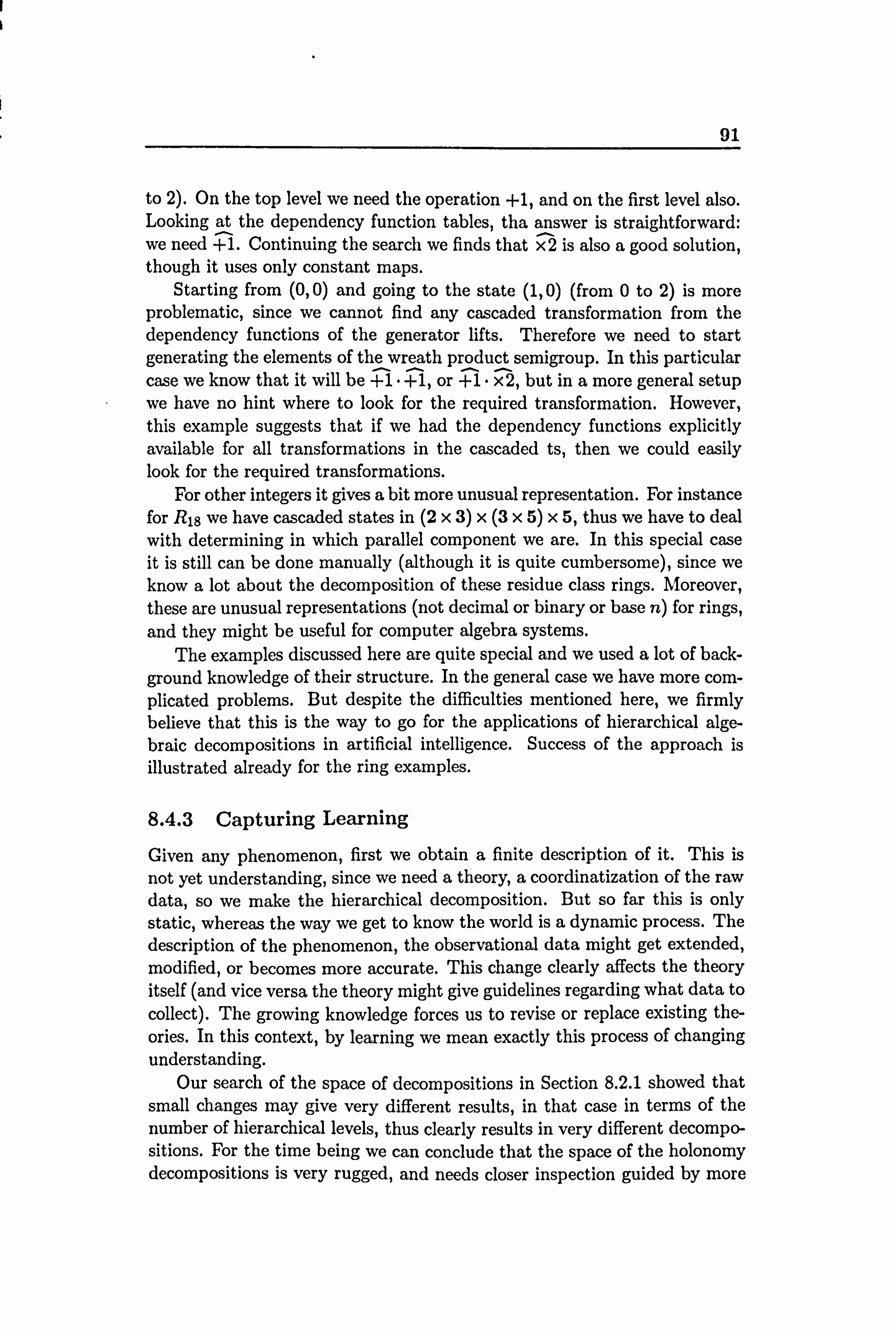
91
to 2). On the top level we need the operation +1, and on the first level also. Looking at the dependency function tables, tha answer is straightforward: we need +1. Continuing the search we finds that x2 is also a good solution, though it uses only constant maps.
Starting from (0,0) and going to the state (1,0) (from 0 to 2) is more problematic, since we cannot find any cascaded transformation from the dependency functions of the generator lifts. Therefore we need to start generating the elements of the wreath product semigroup. In this particular case we know that it will be +1-+1, or +1-x2, but in a more general setup we have no hint where to look for the required transformation. However, this example suggests that if we had the dependency functions explicitly available for all transformations in the cascaded ts, then we could easily look for the required transformations.
For other integers it gives a bit more unusual representation. For instance for R18 we have cascaded states in (2 x 3) x (3 x 5) x 5, thus we have to deal with determining in which parallel component we are. In this special case it is still can be done manually (although it is quite cumbersome), since we know a lot about the decomposition of these residue class rings. Moreover, these are unusual representations (not decimal or binary or base n) for rings, and they might be useful for computer algebra systems.
The examples discussed here are quite special and we used a lot of back- ground knowledge of their structure. In the general case we have more com- plicated problems. But despite the difficulties mentioned here, we firmly believe that this is the way to go for the applications of hierarchical alge- braic decompositions in artificial intelligence. Success of the approach is illustrated already for the ring examples.
8.4.3 Capturing Learning
Given any phenomenon, first we obtain a finite description of it. This is not yet understanding, since we need a theory, a coordinatization of the raw data, so we make the hierarchical decomposition. But so far this is only static, whereas the way we get to know the world is a dynamic process. The description of the phenomenon, the observational data might get extended, modified, or becomes more accurate. This change clearly affects the theory itself (and vice versa the theory might give guidelines regarding what data to collect). The growing knowledge forces us to revise or replace existing the- ories. In this context, by learning we mean exactly this process of changing understanding.
Our search of the space of decompositions in Section 8.2.1 showed that small changes may give very different results, in that case in terms of the number of hierarchical levels, thus clearly results in very different decompo- sitions. For the time being we can conclude that the space of the holonomy decompositions is very rugged, and needs closer inspection guided by more

92 Chapter 8. Applications
specific questions.
8.5 Summary
Here we further deepened our understanding of the holonomy decomposition by studying examples of decompositions in a detailed way. We also showed the difficulties of applying the holonomy decomposition method as the for- mal models of understanding. The results of this chapter give directions for future research.

Chapter 9
Achievements and Future work
9.1 Contributions to Knowledge
At this point, before discussing the possible future directions of this research, we should summarize what has been done in this particular work.
40 Assessing feasibility of computational implementations for the Krohn-Rhodes Theory. Although it is a very difficult problem to generate algebraic decompositions of finite state automata, we have shown that it is doable by using the computational power available on today's computers. At least, for the time being the software tools can provide valuable raw data for the theoretical investigations of the nature of these hierarchical decompositions.
Developing a computational toolkit for the Krohn-Rhodes Theory. Two different proof technique were implemented evaluated in this work: the VUT and the holonomy method. Due to its itera- tive algorithm the VUT method gives such redundant decompositions,
which are not usable except in special cases for some theoretical re- search. Therefore the holonomy method was chosen for a more detailed
study and for a more capable computational implementation.
Detailed study of the hoIonomy decomposition. We have de- scribed a constructive proof of the holonomy decomposition in such a detailed way (several explaining lemmas before bigger proofs, sim- plified notation, etc. ), that understanding the main theorem or devel- oping its computational implementations should be easy after reading this proof. Writing this version of the proof yielded a small but useful theoretical result: in the case of the holonomy decomposition every cascaded state
93

94 Chapter 9. Achievements and Future work
is a lift of some state in the original automaton. This was not known before and it makes a proof shorter.
0 New methods for constructing holonomy group components. During the implementation we developed two different methods (be- yond the trivial brute force solutions) for locating the holonomy groups in the characteristic semigroup. One uses techniques from formal lan- guage theory, while the other one uses the hierarchical dependency structure of the holonomy decomposition.
0 Visualization of the structure of the holonomy decomposi- tion. The automatically generated diagrams (tiling picture, tile au- tomata, etc. ) provide a very easy way of understanding the inner workings of holonomy decomposition.
0 Initial exploration and key examples. With the computational tool available it had become possible to do systematic explorations of the vast space of holonomy decompositions. With random and guided search we could find interesting long decom- positions, we also find a provably sharp upper bound on size of the state set of a holonomy component. Our exploration of finite rings of integers modulo n yielded a nice structural theorem for their decompositions. We present numerous examples, and they serve two different purposes. First, they demonstrate important features of constructions, defini- tions, or proofs. Secondly, some examples pinpoint some crucial prob- lems or give good intuitions, which might be in the focus of the future research.
9.2 Possible Future Research Directions Since there can be many possible research projects utilizing the computa- tional tools for the Krohn-Rhodes Theory, we focus here on those questions of efficient computing of the holonomy decomposition, that have the highest priority.
Efficient partial calculation of 21. In Section 7.3.2 we have shown that we do not need the full extended set of images in order to calculate the holonomy decomposition. However the partial calculation of 71 is not yet solved due to the problem of nonimage tiles (Section 5.7.3).
Relationship between generator sets. The dependency function based method gives us generator sets for the holonomy components, which are comparable to the original generator set regarding their size. But we have to make the relation more precise.

95
Working with coordinates. We showed the potential of holonomy de- compositions to serve as formal models of understanding (buses and trains in Section 8.4.2), but it is still a question how to use its "inter- face" efficiently. We need to find effective algorithms for manipulating coordinates on purpose.
More examples. We still have only considered very few examples of fruit- ful application areas of automated holonomy decompositions.
9.3 Exploring a New Landscape
Philosophy is about questions, not about answers. Any philosophical treatise claiming to have firm answers is suspicious. Science is different, but not entirely. The value of good answers is not doubtful, but good questions pregnant with important answers are also vital for scientific development.
Here we opened up a vast area for further research. As a final phase of developing the Krohn-Rhodes Theory we adapted the holonomy method for a computational implementation. Having a working computational tool is essential for the further development of the theory. Like with telescope or microscope, with the software we can see things which we could not glimpse before. Despite the limitations of the current tool it is already far far beyond the capabilities of the pencil and paper method. Of course, we do not mean replacing the classical mathematical method, we just supply it with more substantial data to work on.
With the computational implementation at hand, now we can ask count- less questions such as 'What is the hierarchical structure of this phenomenon or what are the building blocks of that thing? '. We can examine new aspects of well-known structures, as we did in the case of finite integer residue class rings. Or we can attack problems where our knowledge is close to nothing. For instance observing evolutionary development in artificial life systems needs an understanding of how the individuals reuse and change existing components, measuring the complexity of the evolved organisms.
The holy grail of finite sernigroup theory is determining and efficiently computing Krohn-Rhodes Complexity (or group complexity). The computational tools are clearly not for solving this problem, but seeing actual decompositions, knowing the components may help in determin- ing the KR complexity of particular examples.
As a 'bootstrap' process the computational tool can be used for de- composing well-known structures (as we did in the case of finite residue class rings of integer of modulo n). This might seen to be a 'hide and seek' type game: we hide something in the bush, then happily find it. But meanwhile we can get useful knowledge about how hierarchical structure encodes an understanding of the system.

96 Chapter 9. Achievements and Future work
All we need now is to repeat our starting statement, and after this long trip we made the significance of the sentence should be apparent.
For any finite system a working hierarchical model can be generated au- tomatically.

Appendix A
Decompositions of Finite Residue Class Rings of Integers Modulo n, up to n= 20
The holonomy decompositions of first 20 nontrivial residue class rings of of integers Z. Note that the numbers of levels corresponds to the number of prime factors of n with multiplicities. The number of states at the top hierarchical level (rightmost) equals the sum of primes dividing n. It is also worth noting how the top level components are reused in the decomposition of bigger rings. For instance the top level component of the decomposition of R5 appears in the decompositions of Rio, R15 and R20-
97

98 Appendix A. Decompositions of Finite Residue Class Rings of Integers
Modulo n, up to n= 20
Ring Levels I II -
Holonomy Decomposition R2 1 3 (2, S2) R3 1 4 (3, S3) R4 2 7 (2, C2) 1 (2, C2) R5 1 6 (5, G5: 4) R6 2 12 ((2, C2) x (3, S3)) Z (5, D12) R7 1 8 (7, G7: 6) R8 3 15 (2, S2) 1 (2, S2) 1 (2, S2) R9 2 13 (3, S3) 1 (3, S3)
Rio 2 18 ((2, C2) x (5, G5.4)) 1 (7, Z740)
Ril 1 12 (11, G11: 1o) R12 3 28 (ý2, C2) x (3, S3))I((2, C2) x (5, DI2))1(5, DI2) R13 1 14 (13, G13: 12)
_R14 2 24 ((2, C2) x (7, G7: 6)) 1 (91 084)
R15 2 24 ((3, S3) x (5, G5: 4)) 1 (8, U12o)
R16 4 31 (2, S2) Z (2, S2) 1 (2, S2) 1 (2, S2) R17 1 18 (17,0-1-7: 16)
_RI8 3 39 ((2, C2) x (3, S3)) 1 ((3, S3) x (5, D12)) 1 (5, D12)
Rig 1 20 -
(199 G19: 18) - 3 42 T ((2, C2) x (5 ý
G5: 4)) 1 ((2, C2) x (7, G40)) 1 (7, GL 40)]

Appendix B
Dilworth's Theorem
The following very useful theorem establishes an important connection be- tween the width of a partially ordered set and its chain decomposition. A chain is a subset of the partially ordered set in which every pair of elements is comparable. An antichain is a subset of the partial order in which no two elements are comparable.
Theorem B. 1 (Dilworth's Theorem) Let P= (A, <) be a partial order. Then the minimum number of chains needed to cover A equals the maximum number of elements in an antichain.
The original proof is in [Dil50], and a very short proof can be found in [Tve67]. In the context of directed graphs the theorem is also presented in [BJG02], and in the context of lattices and orders in [DP02].
99

Appendix C
Related Publications
PUBLICATIONS
1. Attila Egri-Nagy, C. L. Nehaniv: Cycle Structure in Automata and the HoIonomy Decomposition, Acta Cybernetica, (in press)
2. Attila Egri-Nagy, C. L. Nehaniv: Algebraic Hierarchical Decom- position of Finite State Automata: Comparison of Implemen- tations for Krohn-Rhodes Theory (poster) CIAA 2004. Ninth International Conference on Implementation and Application of Au- tomata, LNCS 3317.315-316.
CONFERENCE PRESENTATIONS
1. WSA 2005, Workshop on Semigroups and Automata, Joint Satellite Workshop to ICALP'05 and CSL 2005, Lisbon, July 16th, 2005, Fi- nite residue class rings of integers modulo n from the view- point of global semigroup theory
2. CSL2005, International Conference on Semigroups and Languages In Honour of the 65 th birthday of Donald B. McAlister, July 12,13,14 and 15,2005, Lisboa, PORTUGAL, Exploration of the Space of Finite State Automata Using the Holonomy Decomposition
3. BCTCS 2005,21st British Colloquiurn for Theoretical Computer Science, 22-24 March 2005, University of Nottingham, UK, Alge- braic Decompositions of Finite Automata and Formal Models
of Understanding. Abstract published in Bulletin of the European Association for Theoretical Computer Science (EATCS), Number 86,
p246., June 2005.
4. CIAA 2004, Ninth International Conference on Implementation and Application of Automata, Queen's University, Kingston, Ontario, Canada,
100

101
July 22-24,2004, Algebraic Hierarchical Decomposition of Fi- nite State Automata: Comparison of Implementations for Krohn-Rhodes Theory, (poster)
5. CS2, The Fourth Conference of PhD Students in Computer Science, Szeged, Hungary, July 1-4,2004, Holonomy Decomposition of Fi-
nite State Automata
6. MACS 2004,5th Joint Conference on Mathematics and Computer Science June 9-12,2004, Debrecen, Hungary, Algebraic Decompo-
sitions of Finite State Automata and Formal Models of Un- derstanding
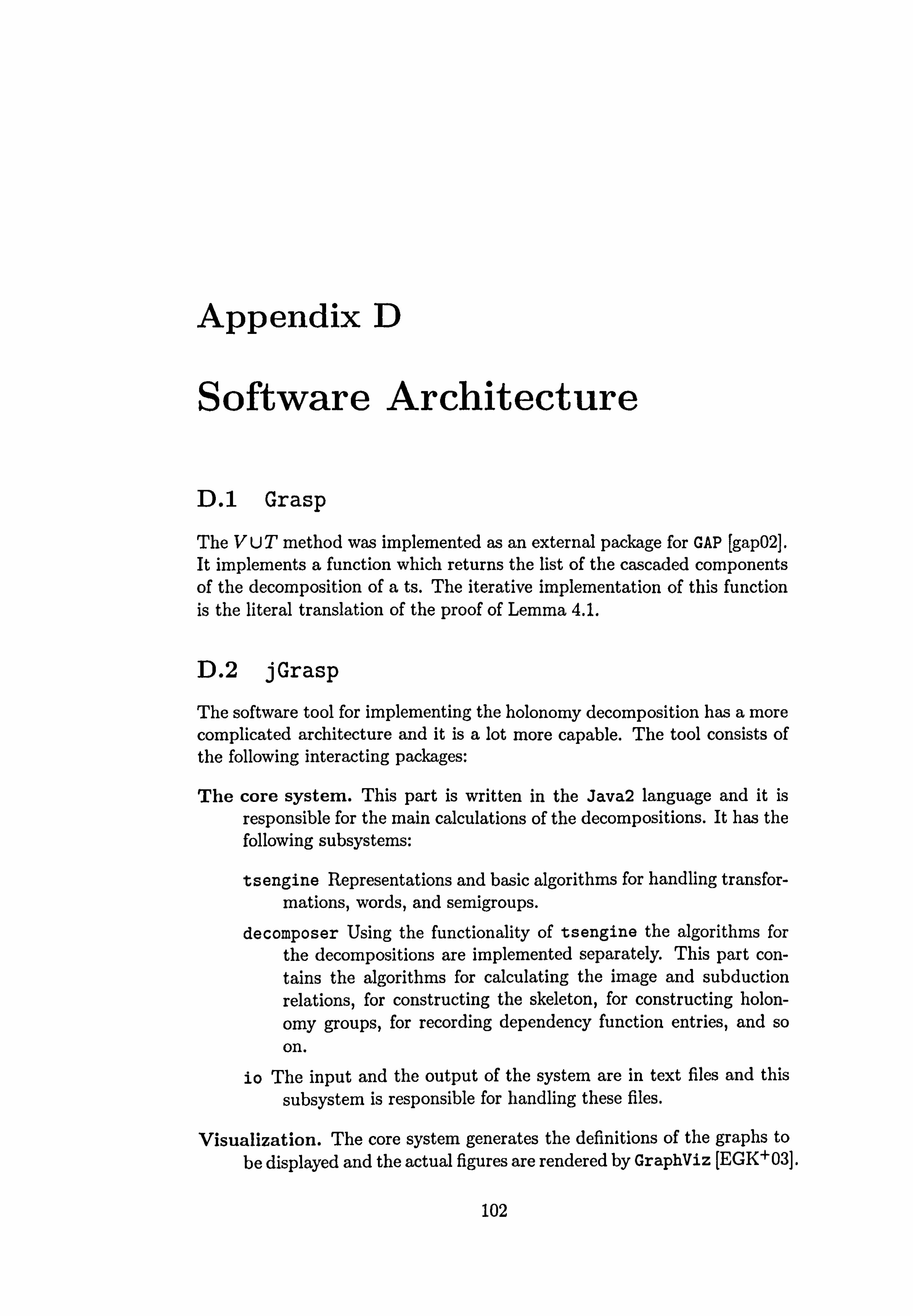
Appendix D
Software Architecture
D. 1 Grasp
The VUT method was implemented as an external package for CAP [gap02]. It implements a function which returns the list of the cascaded components of the decomposition of a ts. The iterative implementation of this function is the literal translation of the proof of Lemma 4.1.
D. 2 jGrasp
The software tool for implementing the holonomy decomposition has a more complicated architecture and it is a lot more capable. The tool consists of the following interacting packages:
The core system. This part is written in the Java2 language and it is responsible for the main calculations of the decompositions. It has the following subsystems:
tsengine Representations and basic algorithms for handling transfor- mations, words, and semigroups.
decomposer Using the functionality of tsengine the algorithms for the decompositions are implemented separately. This part con- tains the algorithms for calculating the image and subduction relations, for constructing the skeleton, for constructing holon-
omy groups, for recording dependency function entries, and so on.
io The input and the output of the system are in text files and this
subsystem is responsible for handling these files.
Visualization. The core system generates the definitions of the graphs to be displayed and the actual figures are rendered by GraphViz [EGK+03].
102

103
Group algorithms. We use GAP for classifying the holonomy group com- ponents.
Execution. The execution of the decomposition and generating the out- put diagrams are coordinated by UNIX shell-scripts.
j Grasp has other functionalities as well (calculating the micro struc- ture of transformations (functional digraphs), exploring one-point mutation neighbourhood of transformation semigroups, etc. ), but currently the main functionality is the decomposition of a ts given by its generator transfor- mations. Future development should concentrate on making the decompo-
sition process more interactively accessible, probably by implementing the core system in GAP.
The latest information about the software toolkits described here can be found on the website http: //graspermachine. sf net.

105
Appendix E
Glossary of Symbols
: 5,: 5, --< subduction, image, tile of relations X11 direct, wreath products
being a lift of a state or transformation the identity element
1A the identity transformation on the set A A, 8 automata AQ the tile automaton of Q BP the set of tiles of P Bi state set of the compoiýent on level i Bi an element of Bi A, B state sets a, b states (A, S), (B, T) transformation semigroups (A, SI) (A, SU 11A})
n the set of integers 10,1, n- 1} Cn the cyclic group on n points D,,, the dihedral group with order n D(A) the state transition graph of A 5
state transition function EQ
union of equivalence classes having elements in BQ f8i dependency function of s on level i Gn: k a semidirect product Cn x Ck GQ
permutator group of Q I the extended set of images HQ holonomy group of Q h(P) the height of P im(t) the image set of transformation t
IC, Iz,
'T Green's relations MP mapping from P to 75
MP mapping from 75 to P P, Q elements of 71

106 Appendix E. Glossary of Symbols
S, T semigroups S, t elements of semigroups (transformations) o, (P, B) selector function &(P, 'B) inverse selector function TA) 7n full transformation semigroup on the set A, on n X, Y alphabets X+, X* the free semigroup, monoid on X XIYIZ input symbols VIW, U words WPQ a witness for P<Q
VfW- the root of word w

Bibliography
[Arb68] Michael A. Arbib, editor. Algebraic Theory of Machines, Lan-
guages, and Semigroups. Academic Press, 1968.
[Ash561 W. Ross Ashby. An Introduction to Cybernetics. Chapman Hall, London, 1956.
[BJG02] Jorgen Bang-Jensen and Gregory Gutin. Digraphs - Theory Algorithms and Applications. Springer, 2002.
[Boo9l] Grady Booch. Object Oriented Analysis and Design with Appli- cations. Benjamin/Cummings Pub. Co., 1991.
[Bro99] Rodney A. Brooks. Cambrian Intelligence: The Early History of the New AL MIT Press (A Bradford Book), 1999.
[CH911 Sang Cho and Dung T. Huynh. Finite-automaton aperiodicity is PSCPACE-complete. Theoretical Computer Science, 88: 99-116, 1991.
[CP67] A. H. Clifford and G. B. Preston. The Algebraic Theory of Semi-
groups (Mathematical Survey, No 7), volume 1 of Mathematical Survey. American Mathematical Society, 2nd edition, 1967.
[Dil50] R. P. Dilworth. A decomposition theorem for partially ordered sets. Annals of Mathematics, 51: 161-166,1950.
[DLM05] Manuel Delgado, Steve Linton, and Jos Morais. GAP package automata. (http: //cmup. fc. up. pt/cmup/mdelgado/automata/)., 2005.
[DN05] PAI D6m8si and Chrystopher L. Nehaniv. Algebraic Theory of Finite Automata Networks: An Introduction, chapter 3, The Krohn-Rhodes and Holonomy Decomposition Theorems. SIAM Series on Discrete Mathematics and Applications, 2005.
[DP02] B. A. Davey and H. A. Priestley. Introduction to Lattices and Order, Second Edition. Cambridge University Press, 2002.
107

108 Bibliography
[EGK+03] J. Ellson, E. R. Gansner, E. Koutsofios, S. C. North, and G. Woodhull. Graphviz and dynagraph - static and dynamic graph drawing tools. In M. Junger and P. Mutzel, editors, Graph Drawing Software, pages 127-148. Springer-Verlag, 2003. http: //www. graphviz. org.
[Eil76] Samuel Eilenberg. Automata, Languages and Machines, vol- ume B. Academic Press, 1976.
[EN02] Gillian Z. Elston and Chrystopher L. Nehaniv. Holonomy em- bedding of arbitrary stable semigroups. International Journal of Algebra and Computation, 12(6): 791-810,2002.
[ENN03] Attila Egri-Nagy and Chrystopher L. Nehaniv. GrasperMachine, Computational Semigroup Theory for Formal Models of Under- standing. (http: //graspermachine. sf net)., 2003.
[ENN04] Attila Egri-Nagy and Chrystopher L. Nehaniv. Algebraic hier- archical decomposition of finite state automata: Comparison of implementations for Krohn-Rhodes Theory. Conference on Im- plementations and Applications of Automata CIAA 2004, Lec- ture Notes in Computer Science, 3317: 315-316,2004.
[tsioo] Zoltan Esik. A proof of the Krohn-Rhodes decomposition theo- rem. Theoretical Computer Science, 234: 287-300,2000.
[gap02] GAP - Groups, Algorithms, and Programming, Version 4.3. (http: //www. gap-system. org)., 2002.
[Gin68] Abraham Ginzburg. Algebraic Theory of Automata. Academic Press, 1968.
[GLS94) Daniel Gorenstein, Richard Lyons, and Ronald Solomon. The Classification of Finite Simple Croups. ANIS, 1994.
(Hal5g] Marshall Hall. The Theory of Groups. The Macmillan Company, New York, 1959.
[HLR88] Karsten Henckell, Susan Lazarus, and John L. Rhodes. Prime decomposition theorem for arbitrary semigroups. Journal of Pure and Applied Algebra, 55: 121-172,1988.
[Hof79] Douglas R. Hofstadter. C6del, Escher, Bach: an Eternal Golden Brain. The Harvester Press Ltd, 1979.
[Ho175] John H. Holland. Adaptation in natural and artificial systems. The University of Michigan Press, Ann Arbor, 1975.

109
[HoI82] W. M. L. Holcombe. Algebraic Automata Theory. Cambridge University Press, 1982.
[Joh0l] Steven Johnson. Emergence. Scribner, 2001.
[Knu98] Donald E. Knuth. The Art of Computer Programming - Sorting and Searching, volume 3. Addison-Wesley, 2nd edition, 1998.
[KR65] Kenneth Krohn and John Rhodes. Algebraic theory of ma- chines. I. Prime decomposition theorem for finite semigroups and machines. Transactions of the American Mathematical So- ciety, 116: 450-464, April 1965.
[KRT68] Kenneth Krohn, John L. Rhodes, and Bret R. Tilson. Algebraic Theory of Machines, Languages, and Semigroups (M. A. Arbib,
ed. ), chapter 5, The Prime Decomposition Theorem of the Al-
gebraic Theory of Machines, pages 81-125. Academic Press, 1968.
[KS98] Stanislav Kublanovsky and Mark Sapir. Potential divisibility in finite semigroups is undecidable. International Journal of Alge- bra and Computation (IJAC), 8(6): 671-680, December 1998.
[LJ80] George Lakoff and Mark Johnson. Metaphors We Live By. Uni-
versity of Chicago Press, 1980.
[LNOO] George Lakoff and Rafael E. Ntinez. Where Mathematics comes from? - How the embodied mind brings mathematics into being. Basic Books, 2000.
[Lot83] M. Lothaire, editor. Combinatorics on Words. Cambridge Uni-
versity Press, 1983.
[MMP+95] 0. Matz, A. Miller, A. Potthoff, W. Thomas, and E. Valkerna. Report on the program AMoRE. Technical Report 9507, Chris- tian Albrecht University of Kiel, October 1995.
[Neh92] Chrystopher L. Nehaniv. Global Sequential Coordinates on Semigroups, Automata, and Infinite Groups. PhD thesis, Uni- versity of California, Berkeley, 1992.
[Neh94] Chrystopher L. Nehaniv. Algebraic engineering of understand- ing: Global hierarchical coordinates on computation for the ma- nipulation of data, knowledge, and process. In Proc. 18th Annual International Computer Software and Applications Conference (COMPSA C 94), pages 418-425. IEEE Computer Society Press, 1994.

110 Bibliography
[Neh96a] Chrystopher L. Nehaniv. Algebra and formal models of under- standing. In Masami Ito, editor, Semigroups, Formal Languages and Computer Systems, volume 960, pages 145-154. Kyoto Re- search Institute for Mathematics Sciences, RIMS Kokyuroku, August 1996.
[Neh96b] Chrystopher L. Nehaniv. A simple, direct proof of the Krohn- Rhodes theorem. In Y. Kobayashi and R. Matsuda, editors, Proceedings of the 20th Symposium on Semigroups, Languages, and Their Related Areas, pages 29-33, Mito, Japan, November 1996.
[NROO] Chrystopher L. Nehaniv and John L. Rhodes. The evolution and understanding of hierarchical complexity in biology from an algebraic perspective. Artificial Life, 6: 45-67,2000.
[Rho7l] John L. Rhodes. Applications of Automata Theory and Alge- bra with the Mathematical Theory of Complexity to Finite-State Physics, Biology, Philosophy, Games, and Codes. University of California at Berkeley, Mathematics Library, 1971.
[RW89a] John L. Rhodes and Pascal Weil. Decomposition techniques for finite sernigroups using categories, L Journal of Pure and Applied Algebra, 62: 269-284,1989.
[RW89b] John L. Rhodes and Pascal Weil. Decomposition techniques for finite sernigroups using categories, IL Journal of Pure and Applied Algebra, 62: 285-312,1989.
[Sch65] M. P. Schiitzenberger. On finite monoids having only trivial subgroups. Information and Control, 8: 190-194,1965.
[Ser03] Akos Seress. Permutation Group Algorithms, volume 152 of Cambridge Tracts in Mathematics. Cambridge University Press, 2003.
[Shy0l] H. J. Shyr. Free monoids and languages. Hon Min Book Com- pany, Taichung, Taiwan, 2001.
[Sim96] Herbert A. Simon. The Sciences of the Artificial - 3rd Edition. MIT Press, 1996.
[Ste03] Luc Steels. Intelligence with representation. Philosophical Transactions: Mathematical, Physical and Engineering Sci-
ences, 361(1811): 2381-2395,2003.
[Tve67] H. Tverberg. On Dilworth's decomposition theorem for partially ordered sets. Journal of Combinatorial Theory, 3: 305-306,1967.

ill
[Zei67] H. Paul Zeiger. Cascade synthesis of finite state machines. In- formation and Control, 10: 419-433,1967. plus erratum.
[Zei68] Paul Zeiger. Algebraic Theory of Machines, Languages, and Semigroups (M. A. Arbib, ed. ), chapter 4, Cascade Decomposi- tion Using Covers, pages 81-125. Academic Press, 1968.