Attenuation of Radio Wave Signals Coupled Into Twelve ... NIST Technical Note 1545 Attenuation of Radio Wave Signals Coupled Into Twelve Large Building Structures C.L. Holloway W.F

NIST Technical Note 1545

Attenuation of Radio Wave Signals Coupled Into Twelve Large Building Structures C.L. Holloway W.F. Young G. Koepke K.A. Remley D. Camell Y. Becquet

U.S. Department of Commerce

Carlos M. Gutierrez, Secretary National Institute of Standards and Technology James Turner, Deputy Director

NIST Technical Note 1545 Attenuation of Radio Wave Signals Coupled Into Twelve Large Building Structures L. Holloway C.L. Holloway W.F. Young G. Koepke K.A. Remley D. Camell Y. Becquet1 Electronics and Electrical Engineering Laboratory National Institute of Standards and Technology 325 Broadway Boulder, CO 80305 1. Chalmers University of Technology, Gothenburg, Sweden August 2008

Certain commercial entities, equipment, or materials may be identified in this document in order to describe an experimental procedure or concept adequately. Such identification does not

imply recommendation or endorsement by the National Institute of Standards and Technology, nor does it

imply that the entities, materials, or equipment are necessarily the best available for the purpose.

National Institute of Standards and Technology Technical Note 1545 Natl. Inst. Stand. Technol. Tech. Note 1545, 240 pages (August 2008)

CODEN: NTNOEF

U.S. Government Printing Office Washington: 2008

For sale by the Superintendent of Documents, U.S. Government Printing Office

Internet bookstore: gpo.gov Phone: 202-512-1800 Fax: 202-512-2250 Mail: Stop SSOP, Washington, DC 20402-0001

iii

Contents

Executive Summary ..................................................................................................................... iv 1. Introduction ............................................................................................................................... 1 2. Frequency Bands ....................................................................................................................... 2 3. Transmitters .............................................................................................................................. 4 4. Receiving Antenna and Measurement System ....................................................................... 5 5. Building Structure Descriptions and Experimental Set-up .................................................. 6

5.1 New Orleans, LA Apartment Building ............................................................................. 6 5.2 Philadelphia, PA Sports Stadium ...................................................................................... 7 5.3 Phoenix, AZ Office Building .............................................................................................. 8 5.4 Colorado Springs, CO CO Hotel Complex ....................................................................... 9 5.5 Boulder, CO Grocery Store ............................................................................................. 10 5.6 Gaithersburg, MD Office Building .................................................................................. 10 5.7 Bethesda, MD Shopping Mall .......................................................................................... 11 5.8 Silver Spring, MD Office Building .................................................................................. 12 5.9 Washington, DC Convention Center .............................................................................. 12 5.10 Boulder, CO Apartment Building ................................................................................. 13 5.11 Commerce City, CO Oil Refinery ................................................................................. 14 5.12 NIST Boulder, CO Laboratory ...................................................................................... 15

6. Experimental Results .............................................................................................................. 16 6.1 New Orleans, LA Apartment Building Results .............................................................. 18 6.2 Philadelphia, PA Sports Stadium Results ....................................................................... 19 6.3 Phoenix, AZ Office Building Results ............................................................................... 19 6.4 Colorado Springs, CO, CO Hotel Complex Results ...................................................... 19 6.5 Boulder, CO Grocery Store Results ................................................................................ 20 6.6 Gaithersburg, MD Office Building Results .................................................................... 20 6.7 Bethesda, MD Shopping Mall Results ............................................................................. 20 6.8 Silver Springs, MD Office Building Results ................................................................... 21 6.9 Washington, DC Convention Center Results ................................................................. 21 6.10 Boulder, CO Apartment Building Results .................................................................... 21 6.11 Commerce City, CO Oil Refinery Results .................................................................... 22 6.12 NIST Boulder, CO Laboratory Results ........................................................................ 22

7. Summary of Results and Conclusions ................................................................................... 22 8. References ................................................................................................................................ 34 9. Figures ...................................................................................................................................... 34

iv

Executive Summary

This is the fourth in a series of NIST Technical Notes (TN) on propagation and detection of radio signals in large building structures (apartment complex, hotel, office building, sports stadium, shopping mall, etc.). The first, second, and third NIST Tech Notes (TN 1540, TN 1541, and TN 1542) described experiments for radio propagation in a structure before, during, and after implosion. The data in these reports give first responders and system designers a better understanding of what to expect from the radio-propagation environment in disaster situations. The goal of this work is to create a large, public-domain data set describing the attenuation of radio signals in various building types in the public safety and cellular telephone bands. With the above goal in mind, measurements were carried out on 12 different large building structures. Frequencies near public safety and cell phone bands as well as ISM and wireless LAN bands (approximately 50 MHz, 150 MHz, 225 MHz, 450 MHz, 900 MHz, 1.8 GHz, 2.4 GHz, and 4.9 GHz) were chosen for these experiments. We carried out these “radio-mapping” experiments to provide data on how radio signals at the different frequencies coupled into the different building structures. Radio transmitters similar to those used by first responders were used, as well as specially designed transmitters for the higher frequencies. These different transmitters were carried throughout various large building structures, while the received signal was recorded at a fixed receive site located outside the large structures. From this we determined the field-strength variability throughout the structures. Transmitters were also carried around the perimeter of the structures with a fixed receiving site on the outside. The results of these signal-strength measurements and the statistical analysis of the data for these radio-mapping experiments are presented here.

Beside plots of the raw datasets, a series of tables that summarize the processed data by frequency bands are presented in this report. This enables easier comparisons between results from different building or structure types. (Note that the exact frequencies are provided in each of the individual site discussions.) Table entries include a building or structure identifier, the actual frequency tested, the specific reference level used to normalize that particular data set, and then median, mean, and standard deviation results for the normalized data. Differences in building types make it difficult to make very strong general statements based on the collected data. However, we do observe some general trends in the data. First, examination of the standard deviation yields some interesting insights. In particular, if we exclude the first receiver site for the NIST laboratory in Boulder, we see that the average standard deviation for the six lower frequency bands ranges from 11.8 dB to 13.4 dB. Limited data were collected for the upper two frequencies; but if we include those results, the upper limit of the range increase to 14.9 dB. Across all eight frequency bands, the range of maximum standard deviation covers 16.8 dB to 22.3 dB, with 22.3 dB occurring at 900 MHz. The minimum standard deviation values range from 3.9 dB to 12.1 dB, with 3.9 dB occurring at 1.8 GHz. Second, in almost all cases, the median value for the power received is less than the average power received. The typical difference is between 2 dB to 3 dB. This suggests that median value may be a better measure for representing the general behavior of the building, or at least a more conservative performance measure.

v

Third, the histograms (which approximate probability density functions, PDFs) and the empirical cumulative density functions (CDFs) do not appear to follow any typical density function. To some extent, each individual test case will generate a unique density. However, the data do not seem to suggest an obvious average or best approximate density function that could be used as a collective representation of the buildings. The data presented in this report aid in understanding the issues faced with first responders communicating into and within large building structures. For example, the large amount of attenuation for the signals coupling into the different structures indicates to system designers what a communication link must overcome in order to provide a reliable system. In addition, the measured signal variability indicates the dynamic environment these different buildings present to a communication system. The results in this report are the fourth in a series of reports detailing experiments performed by NIST in order to provide better understanding of the first responder’s radio propagation environment. The first three reports cover implosion experiments that were performed in three different building structures: an apartment building in New Orleans, LA, a large sports stadium (the “Veterans Stadium”) in Philadelphia, PA, and a convention center in Washington, DC. Looking ahead, other experiments at different frequencies in other building structures are being performed and will be published separately. We will are also performing measurements to simulate and test the performance of adhoc networks in various building structures; the results of these experiments will also be published separately.

1

Attenuation of Radio Wave Signals Coupled Into Twelve Large Building Structures

Christopher L. Holloway, William F. Young, Galen Koepke, Kate A. Remley Dennis Camell, and Yann Becquet

Electromagnetics Division

National Institute of Standards and Technology 325 Broadway, Boulder, CO 80305

In this report, we describe our investigation of radio communication problems faced by emergency responders (firefighters, police, and emergency medical personnel) in disaster situations. A fundamental challenge to communications into and out of large buildings is the strong attenuation of radio signals caused by losses and scattering in the building materials and structure. Besides attenuation, another challenge is the large amount of signal variability that occurs throughout these large structures. We designed experiments in various large building structures in an effort to quantify radio-signal attenuation and variability faced by emergency responders. We carried RF transmitters throughout these structures and placed receiving systems outside the structures. The transmitters were tuned to frequencies near public safety, cell phone bands, and Industrial, Scientific and Medical (ISM) bands, including wireless Local Area Network (LAN) frequencies. This report summarizes the experiments, performed in large building structures. We describe the experiments, detail the measurement system, show primary results of the data collected, and discuss some of the interesting propagation effects we observed. Key words: attenuation; building shielding and coupling; emergency responders; radio communications; radio propagation experiments; signal variability; weak-signal detection

1. Introduction

When emergency responders enter large structures (e.g., apartment and office buildings, sports stadiums, stores, malls, hotels, convention centers, warehouses, etc.) communication to individuals on the outside is often impaired. Cellular telephones and mobile-radio signal strength is reduced due to (a) attenuation caused by propagation through the building materials, and (b) scattering by the building geometry [1-8]. Also, the large amount of signal variability throughout the structures causes degradation in communication systems. Here, we report on a National Institute of Standards and Technology (NIST) project to investigate communications problems faced by first responders (firefighters, police and emergency medical personnel) in disaster situations involving large building structures. As part of this effort, we are investigating the propagation and coupling of radio waves into large building structures. This report covers experiments that utilized a single-frequency, unmodulated carrier, whereas a companion report, NIST Technical Note 1546 [9], describes measurements

2

that support increased understanding of modulated signal transmissions for the public-safety sector. The experiments reported here were performed in 12 different large building structures and are essentially measurements of the reduction in radio-signal strength caused by propagation through the structures. These structures include four office buildings, two apartment buildings, a hotel, a grocery store, a shopping mall, a convention center, a sports stadium, and an oil refinery. In order to study the radio characteristics of these structures at the various frequencies of interest to first responders, frequencies near public-safety and cell phone bands, as well as ISM and wireless LAN bands (approximately 50 MHz, 150 MHz, 225 MHz, 450 MHz, 900 MHz, 1.8 GHz, 2.4 GHz, 4.9 GHz) were chosen. A detailed description of the transmitters we used is given in detail in Section 3. The experiments performed here are referred to as “radio mappings.” This involved carrying transmitters (or radios) tuned to various frequencies throughout the 12 structures while recording the received unmodulated signal at a site located outside the building. The reference for these data was a direct, unobstructed, line-of-sight signal-strength measurement with the transmitters external to the different structures and in front of the receiving antennas. The purpose of the radio-mapping measurements was to investigate how the signals at the different frequencies couple into the structures, and to determine the field-strength variability throughout the structures. A detailed description of the measurement system and antennas is given in Section 4. This report is organized as follows: Section 2 describes the frequencies used in these experiments. Section 3 discusses the transmitters, and Section 4 describes the automated measurement system used in the radio-mapping and propagation measurements. In Section 5, we describe the different structures and detail our experimental procedures for each structure. In Section 6, we present the data collected at various stages of the experiment. Finally, in Section 7, we summarize the results of these experiments and discuss some of the interesting propagation effects observed.

2. Frequency Bands

An overview of the frequencies used by the public-safety community nationwide (federal, state, and local) is given in Table 1, which shows a broad range of frequencies ranging from 30 MHz to 4.9 GHz. The modulation scheme has historically been analog FM, but this is slowly changing to digital as Project 25 radios come online [10]. The modulation bandwidth in the VHF and UHF bands has been 25 kHz, but due to the need for additional communications channels in an already crowded spectrum, most new bandwidth allocations are 12.5 kHz. The older bandwidth allocations will gradually be required to move to narrow bandwidths to increase the user density even further. The crowded spectrum and limited bandwidth are also pushing the move to higher frequency bands in order to support new data-intensive technologies. The cellular phone bands are summarized in Table 2.

3

As shown in Table 1, frequencies currently used by public safety and other emergency responders and cellular telephones are typically below 2 GHz. New frequency allocations and systems, including higher frequencies (e.g., around 4.9 GHz), will become increasingly important in the future. We chose eight frequency bands below 5 GHz, from about 50 MHz to 4.9 GHz. These include four VHF bands typically used for analog FM voice, one band used for multiple technologies (analog FM voice, digital trunked FM, and cellular telephone), one band near the digital cellular telephone band, and wireless LAN bands.

Table 1. Public safety community frequencies.

Frequency band

(MHz) Description

30-50 Used mainly by highway patrols for long-distance propagation; currently being phased out

150-174 Local police and fire. Lower frequency preferred because of its better long-distance propagation quality

406-470 Used by federal officers and others 700-800 Used in urban areas 800-869 Primarily urban usage

4900 A newly allocated band with 50 MHz bandwidth for sending images and broadband data

Table 2. Cellular Phone Frequencies

Frequency band

(MHz) Description

800 AMPS or analog systems, migrating to digital trunked and point-to-point communications

1900 PCS or digital system

In designing an experiment to investigate the signal penetration characteristics into large buildings at these different frequency bands, we chose frequencies very close, but not identical, to the above bands. If frequencies were chosen in the public safety or commercial land-mobile bands, interference to the public safety and cellular systems could possibly occur. Conversely, these existing systems could interfere with our experimental setup. In addition, obtaining frequency authorizations in these bands for our experiments would have been problematic due to the intense crowding of the spectrum. To circumvent these issues, we were able to receive temporary authorization to use frequencies in the U.S. Government frequency bands adjacent to these public safety bands. Table 3 lists the frequency bands that were used in the experiments. The lower four bands correspond to the frequencies used by the public-safety community; 902 MHz can be associated with several services including both public safety and cellular phones; the highest frequency is near the digital cellular phone and wireless LAN bands. The exact

4

frequencies varied depending on which city the experiments were performed. Section 5 describes the different structures and the exact frequencies used in each experiment.

Table 3. Frequency bands used in the experiments.

Frequency band (MHz)

Description

49 Simulate a public safety band 162 Simulate a public safety band 226 Simulate a public safety band 448 Simulate a public safety band 902 Simulate a public safety or cellular phone band

1830 Simulate a cellular phone band 2450 Wireless LAN 4900 Recently allocated with 50 MHz bandwidth for sending images and

broadband data

3. Transmitters

The design requirements for the transmitters used in the experiments discussed here were that they should: (1) transmit an unmodulated carrier at the frequencies listed in the tables above, (2) operate continuously for several hours, and (3) be portable. To accomplish this, two different types of transmitters were chosen. For the four lower frequency bands (the VHF/UHF public-safety bands), off-the-shelf amateur radios were modified. The modifications included: (1) reprogramming the frequency synthesizer to permit transmitting at government frequencies, (2) disabling the transmitter time-out mode in order to allow for continuous transmission, and (3) connecting a large external battery pack. The specifications of these modified radios then had to be reported to the National Telecommunications and Information Administration (NTIA) frequency coordinator in order to obtain approval for use in government frequency bands. With the larger battery packs, the modified radios could transmit continuously for 12 h to 18 h at an output power of 1 W. The extended transmitting time required us to provide additional cooling since the radios were designed for typical communications, that is, to transmit intermittently with cooling time between transmissions. This was accomplished with cooling fans. The stability and radiated power from these inexpensive radios was measured over a 24 h period. The modified radios and battery packs were placed in durable orange plastic cases for mobility. The antennas could be mounted either inside or outside the plastic cases. For these measurements, the antennas were mounted on the outside of the cases. Figure 1 shows the final arrangement of modified transmitters used for the lower four frequency bands. This figure shows one modified transmitter placed in an orange plastic case.

5

Commercial transmitters were available for the higher frequency bands (900 MHz, 1800 MHz, 2.4 GHz, and 4.9 GHz). These off-the-shelf transmitters were already in plastic protective cases and could transmit continuously for 12 h. Figure 2 shows these transmitters. Note that the cases for the higher-frequency transmitters were not orange, but grey. 4. Receiving Antenna and Measurement System

The receiving system is sketched in Figure 3. We assembled four antennas on a 4 m mast, as illustrated. The radio-frequency output from each antenna was fed through a 4:1 broadband power combiner. This arrangement gave us a single input to our portable spectrum analyzers, which could then scan over all the frequencies of interest without switching antennas. The four antennas were chosen to be optimal (or at least practical) for each of the frequency bands we were measuring. The selected antennas were an end-fed vertical omnidirectional antenna for 50 MHz, a log-periodic-dipole-array (LPDA) for the 160 MHz, 225 MHz, and 450 MHz bands, and Yagi-Uda arrays for 900 MHz and 1830 MHz. Horn antennas were used for the 2.4 GHz and 4.9 GHz frequency bands. This assembly could then be mounted on a fixed tripod at one of the listening sites, or it could be inserted into a modified garden cart for portable measurements (see Figure 4 and Figure 5). The receiving sites contained, in addition to the antenna system, a generator, uninterruptible power supply (UPS), spectrum analyzer, global positioning system (GPS) receiver, computer, and associated cabling. Photos of the antenna assembly mounted on a tripod and mounted on the mobile cart are shown in Figure 4 and Figure 5. As shown in Figure 3, the measurement system consists of a portable spectrum analyzer, GPS receiver, and a laptop computer. The data collection process was automated by use of a graphical programming language. This software was designed to control the analyzer, and to collect, process, and save data at the maximum throughput of the equipment. The software controlled the spectrum analyzer via an IEEE-488 interface bus and the GPS receiver via a serial interface. The GPS information was used to record the position of the receiving sites during the measurements. The software was written to maximize throughput of the data collection process and to run for an undefined time interval. This was achieved by running as parallel processes the collecting, processing, and saving of the data for post-collection processing. The data were continuously read from the spectrum analyzer at its optimal settings and stored in data buffers. These buffers were read and processed for each signal and displayed for operator viewing. The processed data were then stored in additional buffers to be re-sorted and saved to a file on disk. The initial setup of the parameters for the spectrum analyzer determined the quality of optimization for this process. There were several instrument parameters that were critical during the setup, including the analyzer sweep time, resolution bandwidth, and frequency span of the spectrum analyzer trace. The number and spread of the test frequencies in a particular band influenced the allowed range of adjustment for these parameters. These two factors also influenced the number of traces necessary to cover all the test frequencies. Interference from signals in the adjacent spectrum influenced the instrument setup and data collection speed by forcing smaller resolution bandwidths. The reference level for each trace was also checked and

6

adjusted during the measurement to improve the resolution and accuracy of the power level reading. All of these factors had some effect on the sampling rate. The sampling rate of the complete measurement sequence was the major factor in how much spatial resolution we had during walk-through or field-mapping experiments (we also had some flexibility in our walking speed) and the time resolution for recording the signals. We used three different models of spectrum analyzers, each having a different sampling rate ranging from about 0.5 s to 7 s, to measure all 20 frequencies in the 6 frequency bands. The frequencies were spaced such that we could utilize one spectrum analyzer trace for each band. The reason for the relatively large sampling range is that the first four experiments (New Orleans through the Colorado Springs, CO hotel complex) collected data for all frequencies during a single walk-through. For the remaining eight experiments, only a single frequency was collected during each walk-through, i.e., each frequency required a walk-through. These rates were achieved only after optimizing the instrument control and data transfer processes mentioned above. The data from the spectrum analyzer trace were saved in binary format to disk (to allow us to reprocess the raw data at a later time if needed); they were then processed to extract the signals at each particular frequency. These results were then put into a spreadsheet file and saved with other measurement information. The sampling rates were sufficient for the field-mapping experiments (if we did not walk too fast).

5. Building Structure Descriptions and Experimental Set-up This section briefly describes the 12 different large building structures used in these experiments and details the experimental set-up. These structures include four office buildings, two apartment buildings, a hotel, a grocery store, a shopping mall, a convention center, a sports stadium, and an oil refinery.

5.1 New Orleans, LA Apartment Building The building for this set of radio propagation experiments was a 13-story apartment complex located in a suburb of New Orleans, LA (Figure 6), specifically, the William J. Fisher building on Whitney Ave. We performed the radio-mapping measurements prior to the scheduled implosion of the structure. We also performed measurements before, during, and after the implosion of this structure; and details of these implosion measurements are reported in Reference [5]. The 13 stories included a ground-level commons area and parking, and 12 floors with 14 efficiency apartments on each floor. The individual apartments on each level opened to a common outside hallway on the west side of the building. There was an elevator control and maintenance room in a penthouse on the roof of the building. This space was accessed by a metal spiral staircase on the top floor. There were two internal passenger elevators and one external freight elevator near the center of the building. Two external stairwells near each end of the building accessed all floors. There was no basement in this building.

7

The building was constructed of reinforced concrete, steel, and standard interior finish materials. Significant demolition was already completed when we arrived; all plumbing fixtures, most glass windows and doors, and the contents of the apartments had been removed. The reinforced concrete walls on the lower two levels had been cut away, leaving only support columns remaining. The ground level commons area structure had been demolished and the debris in the area removed. Material had been judiciously removed from certain structural parts of the lower levels, including stairwells and elevator shafts to facilitate a proper collapse during the implosion. Figure 7 shows a few photos of the building interior as it existed during the experiments. The pre-implosion preparation and partial demolition on the lower levels is visible in several of the photos. Figure 8 shows a drawing of the structure. The purpose of these measurements was to investigate how signals at the different frequencies couple into the building and to determine the field strength variability throughout the building. For the radio-mapping experiments, one fixed receiving site (as described above) was assembled on the northeast side of the building (see Figure 8), approximately 30 m from the northeast corner of the building. During this experiment, the transmitters were carried throughout the building and the received signal levels were recorded. As the received signal was recorded, the location of the transmitters in the buildings was also recorded. The frequencies used in the experiment are shown in Table 4.

Table 4. Frequencies used in the New Orleans, LA apartment building experiments.

Frequency band Description

49.60 MHz Simulate a public safety band 162.00 MHz Simulate a public safety band

225.375 MHz Simulate a public safety band 448.60 MHz Simulate a public safety band 902.60 MHz Simulate a public safety or cellular phone band

1832.50 MHz Simulate a cellular phone band

5.2 Philadelphia, PA Sports Stadium The next structure for the radio propagation experiments was Veterans Stadium, a large sports arena in Philadelphia, PA (see Figure 9). We performed the radio-mapping measurements prior to the scheduled implosion of the structure. We also performed measurements before, during, and after the implosion of this structure, and details of these implosion measurements are reported in Reference [7]. The nearly circular stadium was constructed of reinforced concrete, steel, and standard interior finish materials. Figure 10 show details of the original stadium and some of the preparations and partial demolition of the different sections of the stadium. As shown in these figures, the stadium had multiple levels with large open areas. The exterior perimeter of the stadium was approximately 805 m (1/2 mi). Since this structure was also scheduled for implosion, significant

8

demolition had already been completed when we arrived; all plumbing fixtures, most glass windows and doors, and other contents had been removed. Material had been judiciously removed from certain structural parts of the lower levels including stairwells and elevator shafts to facilitate a proper collapse during the implosion. Figure 11 shows a plan of the structure and approximate locations of the transmitter and receive instruments. The purpose of these measurements was to investigate how signals at the different frequencies couple into the stadium and to determine the variability in field strength throughout the stadium. Also, by carrying the transmitters around the exterior perimeter of the stadium the amount of signal blockage caused by the stadium from one side to the other could be investigated. For the radio-mapping experiments, one fixed receiving site (as described above) was assembled on the southwest perimeter of the stadium (see Figure 11), approximately 53 m from Column #10. During this experiment, the transmitters were carried (and at times, driven aboard an all-terrain vehicle or ATV) throughout the stadium and the received signal levels were recorded. Measurements were performed with the receiving antennas polarized in both the horizontal and vertical direction (with respect to the ground). As the received signal was recorded, the location of the transmitters in the buildings was also recorded. The frequencies used in the experiment are shown in Table 5.

Table 5. Frequencies used in the Philadelphia sports stadium experiments.

Frequency band

(MHz) Description

49.60 Simulates a public safety band 162.09 Simulates a public safety band 225.30 Simulates a public safety band 448.50 Simulates a public safety band 902.45 Simulates a public safety or cellular phone band 1832.00 Simulates a cellular phone band

5.3 Phoenix, AZ Office Building

The building was an eight-story office building located in Phoenix, AZ at 2375 East Camelback Rd.(Figure 12). There were two sub-basements in the building. The building was constructed of steel with a large number of windows and standard interior-finish materials. The building was fully furnished with office furniture. Measurements were performed during daytime hours. As a result, people were moving throughout the building during the experiments. Figure 13 shows some interior photos of the office building. For the radio-mapping experiments, one fixed receiving site (as described above) was assembled on the west side of the office building (see Figure 14), approximately 50 m from the front door. During this experiment, the transmitters were carried throughout the building, including the roof and the two sub-basements, and the received signal levels were recorded. Measurements were

9

performed with the receiving antennas polarized in the vertical direction. As the received signal was recorded, the location of the transmitters in the office buildings was also recorded. The frequencies used in the experiment are shown in Table 6.

Table 6. Frequencies used in the Phoenix, AZ office building experiments.

Frequency band

(MHz) Description

154.07 Simulates a public safety band 765 Simulates a public safety band 867 Simulates a cellular phone band

5.4 Colorado Springs, CO, CO Hotel Complex

The building was a 14-story hotel complex located in Colorado Springs, CO, CO (Figure 15). At the time of the measurements, the complex was referred to as the Antlers: Adam’s Mark Hotel. The complex had three sub-level parking garages. The complex also had a small conference facility and stores located in the structure. The building was constructed of reinforced concrete and standard interior-finish materials. The building was fully furnished during the experiments. Measurements were performed during daytime hours and, as a result, people were moving throughout the building during the experiments. Figure 16 shows some interior photos of the hotel complex building. For the radio-mapping experiments, two fixed receiving sites (as described above) were assembled on the outside of the structure (see Figure 17). One was approximately 50 m from the front door, and a similar receiving site was set up in a parking lot near the southwest corner of the building, approximately 30 m from the corner of the building. During this experiment, the transmitters were carried throughout the complex, including the three sub-level parking garages, and the received signal levels were recorded. Measurements were performed with the receiving antennas polarized in both the vertical and horizontal directions. As the received signal was recorded, the location of the transmitters in the hotel was also recorded. The frequencies used in the experiment are shown in Table 7.

Table 7. Frequencies used in the Colorado Springs, CO, CO hotel complex experiments.

Frequency band

(MHz) Description


10

5.5 Boulder, CO Grocery Store The building was a one-story grocery store located in Boulder, CO (Figure 18). This was the King Soopers grocery store located at Table Mesa Dr. and Broadway St. The grocery was constructed of brick and steel. The store was fully furnished during the experiments. Measurements were performed during daytime hours and, as a result, people were moving throughout the store during the experiments. Figure 19 shows some interior photos of the building. For the radio-mapping experiments, one fixed receiving site (as described above) was assembled on the northwest side of the store building (see Figure 20), approximately 30 m from front door. During this experiment, the transmitters were carried throughout the store as well as around the outside perimeter. Measurements were performed with the receiving antennas polarized in the vertical direction. As the received signals were recorded, the location of the transmitters in the store was also recorded. The frequencies used in the experiment are shown in Table 8.

Table 8. Frequencies used in the Boulder, CO grocery store experiments.

Frequency band

(MHz) Description


5.6 Gaithersburg, MD Office Building

The building was a ten-story office building at the NIST facility in Gaithersburg, MD (Figure 21). The building was constructed of reinforced concrete. The building was fully furnished during the experiments. Measurements were performed during daytime hours and, as a result, people were moving throughout the structure during the experiments. For the radio-mapping experiments, one fixed receiving site (as described above) was assembled on the southeast side of the store building (see Figure 22), approximately 60 m from the front door. During this experiment, the transmitters were carried throughout the building. Measurements were performed with the receiving antennas polarized in the vertical direction. As the received signals were recorded, the location of the transmitters in the store was also recorded. The frequencies used in the experiment are shown in Table 9.

11

Table 9. Frequencies used in the Gaithersburg, MD office building experiments.

Frequency band

(MHz) Description


5.7 Bethesda, MD Shopping Mall

The Montgomery Mall was a two-level shopping mall in Bethesda, MD (Figure 23). The building was constructed of reinforced concrete and brick. The building was fully furnished during the experiments. Measurements were performed during daytime hours and, as a result, people were moving throughout the structure during the experiments. Figure 24 shows some internal photos of the mall complex. For the radio-mapping experiments, two fixed receiving sites (as described above) were assembled on both the east and west sides of the mall (see Figure 25), approximately 60 m from the two entrances. During this experiment, the transmitters were carried throughout the mall. Measurements were performed with the receiving antennas polarized in the vertical polarization. As the received signal was recorded, the location of the transmitters in the store was also recorded. The frequencies used in the experiment are shown in Table 10. This is a two-level facility and during the walk-throughs we stopped at predetermined locations on both the upper and lower levels. An internal floor plan with these locations is shown in Figure 26. The green arrows in the figure represent the actual paths that were walked.

Table 10. Frequencies used in the Bethesda, MD shopping mall experiments.

Frequency band

(MHz) Description


12

5.8 Silver Spring, MD Office Building

The building was the 11-story Discovery office building in Silver Spring, MD (Figure 27). The building was constructed of concrete, steel, and glass. The building included a three-level underground parking garage. The building had been recently built and most rooms were furnished with cubicle dividers and typical office furniture, while some were essentially empty. As in earlier measurements, there were people moving about in the structure during the tests in the occupied sections of the building. Figure 28 shows some internal photos of the office building. This structure consisted of two adjoining units or buildings. While walking through the building, we stopped at the various locations on each floor and as well as at the corridor adjoining the two buildings. Each stop is labeled with letters A-I in Figure 29 and on the curves in the next section.

For the radio-mapping experiments, one fixed receiving site (as described above) was assembled on the east side of the building (see Figure 30), approximately 20 m from the main entrance. During this experiment, the transmitters were carried throughout the building, including the three-level underground parking garage. Measurements were performed with the receiving antennas polarized in the vertical direction. As the received signals were recorded, the location of the transmitters in the store was also recorded. The frequencies used in the experiment are shown in Table 11.

Table 11. Frequencies used in the Silver Spring, MD Discovery office building experiments.

Frequency band

(MHz) Description


5.9 Washington, DC Convention Center

The structure in the experiment was the old Washington, DC Convention Center (see Figure 31). We performed these radio-mapping measurements prior to the scheduled implosion of the structure. We also performed measurements before, during, and after the implosion of this structure, and details of these implosion measurements are reported in Reference [8]. This massive two-level structure was constructed of reinforced concrete, steel, and standard interior finish materials. Figure 32 shows some internal photos of the convention center. As shown in Figure 31, the convention center had two large levels with three levels of offices. This

13

structure was scheduled for demolition and significant demolition had already been completed when we arrived; all plumbing fixtures, most glass windows and doors, and other contents had been removed. Figure 33 shows the locations of the three receive sites for the experiments. These three fixed receiving sites were assembled on the perimeter of the convention center. Receiving site RX 1 was placed approximately 23 m (75 ft) from the northwest perimeter of the convention center. Receiving site RX 2 was placed approximately 23 m (75 ft) from the northeast perimeter of the convention center. Receiving site RX 3 was placed approximately 15 m (50 ft) from the southeast perimeter of the convention center. During these experiments, the transmitters were carried throughout the convention center, and the received signal levels were recorded. Measurements were performed with the receiving antennas polarized in the vertical direction (with respect to the ground). As the received signals were recorded, the locations of the transmitters in the convention center were also recorded. The frequencies used in the experiment are shown in Table 12.

Table 12. Frequencies used in the Washington DC convention center experiments.

Frequency band

(MHz) Description


5.10 Boulder, CO Apartment Building

The building was the 11-story Horizon West apartment building in Boulder, CO (Figure 34). The building was constructed of reinforced concrete, steel, and brick with standard interior-finish materials. The building was fully furnished and occupied during the experiments. Measurements were performed during daytime hours and, as a result, people were moving throughout the building during the experiments. Figure 35 and Figure 36 show the two receiver setups at Horizon West, while Figure 37 displays internal photos of the apartment building. For the radio-mapping experiments, two fixed receiving sites (see Figure 35) were assembled on the east side and north side of the apartment building, approximately 60 m and 80 m from the apartment building. During these experiments, the transmitters were carried throughout the building. Measurements were performed with the receiving antennas polarized in the vertical direction. As the received signal was recorded, the location of the transmitters in the apartment building was also recorded. The frequencies used in the experiment are shown in Table 13.

14

Table 13. Frequencies used in the Boulder, CO apartment building experiments

Frequency band

(MHz) Description

162.075 Simulates a public safety band 230.0 Simulates a public safety band 439.25 Simulates a public safety band 908.0 Simulates a public safety or cellular phone band 1830.0 Simulates a cellular phone band 2445.0 Simulates a wireless LAN 4900.0 Simulates a public safety band

5.11 Commerce City, CO Oil Refinery The facility was the SUNCOR Energy oil refinery in Commerce City, CO (Figure 38). The refinery was basically an outdoor facility with several intricate piping systems. Measurements were performed during daytime hours and, as a result, people were moving throughout the refinery. During these experiments, the transmitters were carried throughout the refinery. There were two paths chosen for these tests, one through the center of the processing section with dense piping, and the other around the cluster of large metal storage tanks. During the measurements, the transmitters were carried throughout the dense piping system and driven around the large storage tanks. Figure 39 and Figure 40 show some photos of the refinery complex in which the transmitters were carried, while Figure 41 shows the driven section of the refinery during the data collection process. For the radio-mapping experiments, two fixed receiving sites (as described above) were assembled on the south side and north side of the refinery complex (see Figure 42), approximately 100 m and 30 m from the piping structures. The green arrows in the figure represent the actual paths that were walked. Measurements were performed with the receiving antennas polarized in the vertical direction. As the received signals were recorded, the location of the transmitters in the refinery complex was also recorded. The frequencies used in the experiment are shown in Table 14.

15

Table 14. Frequencies used in the Commerce City, CO oil refinery complex experiments.

Frequency band

(MHz) Description

49.85 Simulates a public safety band 162.075 Simulates a public safety band

230.0 Simulates a public safety band 439.25 Simulates a public safety band 908.0 Simulates a public safety or cellular phone band 1830.1 Simulates a cellular phone band 2445.0 Simulates a wireless LAN 4900.0 Simulates a public safety band

5.12 NIST Boulder, CO Laboratory

This building was the main building (referred to as the Radio Building) at the NIST laboratories in Boulder, CO (see Figure 43). The building is constructed of reinforced concrete and is basically a four-story building. However, the building is built on a hillside, and consequently, some locations in the building are below ground level. Measurements were performed during daytime hours and, as a result, people were moving throughout the building during the experiments. For the radio-mapping experiments, two fixed receiving sites (as described above) were assembled on the south side of the laboratory building (see Figure 44 and Figure 45). The receive site at Wing 4 was located on the landing dock, while the receive site at Wing 6 was approximately 10 m from the building. During these experiments, the transmitters were carried throughout the laboratory. Measurements were performed with the receiving antennas polarized in the vertical direction. As the received signals were recorded, the location of the transmitters in the buildings was also recorded. The frequencies used in the experiment are shown in Table 15.

16

Table 15. Frequencies used in the NIST Boulder laboratory experiments.

Frequency band

(MHz) Description

49.8 Simulates a public safety band 162.075 Simulates a public safety band 230.0 Simulates a public safety band 439.25 Simulates a public safety band 908.0 Simulates a public safety or cellular phone band 1830.0 Simulates a cellular phone band 2445.0 Simulates a wireless LAN 4900.0 Simulates a public safety band 6. Experimental Results

In this section the measured data are presented from several perspectives. The section is divided into subsections, with each subsection discussing a different set of building structure measurements. Plots of the walk-through data, normalized to a reference point, are provided for the investigated frequencies, and the appropriate figure numbers are indicated in the subsection discussions. Plots of the walk-through data statistics are also included. General descriptions of the experimental setups for the various sites were provided earlier in Sections 4 and 5. Any unique features of a site that appear to impact the collected data are pointed out in the appropriate results subsection. The common acronyms and abbreviations used in the labeling of the walk-through figures and statistical plots are provided in Table 16.

17

Table 16. Common abbreviations used in the statistic tables and data igures

Acronym or Abbreviation Meaning Apmt. Apartment

Approx. Approximate Col. Column

Fl., FL, fl. Floor Freq. Frequency Horiz. Horizontal LOS line-of-site Lx Level x or floor x, where x is a number N North

N.E. Northeast N.W. Northwest Ref. Reference signal level

Polar. Polarization S South

Std. dev. Standard deviation S.E. Southeast S.W. Southwest Vert. Vertical

The collected data are plotted as a power level versus the sample number, where the sample number corresponds to different locations in the building structure. The power level is normalized to a reference signal, which is collected at a location with line-of-sight to the receiver. Note that the reference level was not always the strongest measured signal level. Also, in a few cases, a line-sight-sight reference was not available, and an average of near-maximum values was utilized as the reference value instead. This difference in reference level does not affect the variability of the signal level, but does impact the median and the mean. The histograms are created by use of a bin width of 1 dB, and are based on normalized received signal power levels. Median, mean, and standard deviation statistics are also calculated based on the normalized decibel values of the measured data. We will present the data collected for each building in the chronological order in which it was collected. The data are presented in two forms. First, we present the received power levels versus location in the particular building structure. Second, we present the data in a statistical manner using histograms and cumulative density functions (CDFs). After we have presented all the data for each building, the next section summarizes the data from all 12 buildings as a whole, and we draw a few conclusions.

18

6.1 New Orleans, LA Apartment Building Results The apartment building in New Orleans, LA provided the first set of data collected (in chronological order). Plots of the signal power versus sample number are provided for the six lower-frequency bands in Figure 46 to Figure 51. Corresponding histograms and empirical cumulative density functions (CDFs) are found in Figure 52 and Figure 53. In these experiments, approximately 500 samples were collected for each frequency over the complete building walk-through, and the time between samples was approximately 6 s. The reference level for the six frequencies is much higher than that used in most subsequent experiments, which suggests a starting location quite close to the receiver site. As we will see, the standard deviation results are quite similar to results from the other buildings. Also, this particular building had been prepared for demolition, and thus did not contain material such as window glass. This removal of substantial portions of building material, as well as internal content, may have impacted the data. We also performed measurements before, during, and after the implosion of this structure and details of these implosion measurements are reported in Reference [5]. 6.2 Philadelphia, PA Sports Stadium Results A large sports stadium was the second structure investigated. The data collected consisted of a walk-through within the stadium and around the exterior of the stadium for both horizontal and vertical antenna polarizations at the receiver. A sampling rate of approximately 6 s per frequency resulted in small numbers of samples corresponding to a large geographic area or path length. The limited number of sample points over a long path distance does not provide a high resolution of the signal power behavior. Also, the data shown are normalized to a 0 dBm reference level (all other results do not utilize a normalized reference level). The data for both the interior and exterior of the stadium are given in Figures 54 through 92. The walk-through plots for the interior of the stadium are found in Figure 54 to Figure 59 (horizontal polarization), Figure 62 to Figure 67 (horizontal polarization), and Figure 70 to Figure 75 (vertical polarization). Statistical plots corresponding to these three sets of figures are found in Figure 60 and Figure 61, Figure 68 and Figure 69, and Figure 76 and Figure 77. Note that the two inside walk-throughs with horizontal polarization do not directly concatenate, but in general, the combination of the two walk-throughs covers the same path as the single vertical polarization inside walk-through. Stadium exterior walk-through plots are found in Figure 78 to Figure 83 (horizontal polarization), and Figure 86 to Figure 91 (vertical polarization). The corresponding statistical plots are shown in Figure 84 and Figure 85 and Figure 92 and 93, respectively. The most noticeable difference between the five cases is that for all frequencies above 50 MHz, the median of the outside walk with the vertical polarization is at least 3.9 dB worse than the four other walks. The standard deviation is also greater than 18.4 dB for all frequencies for the vertical polarization outside walk. We also performed measurements before, during, and after the implosion of this structure, and details of these implosion measurements are reported in Reference [7].

19

6.3 Phoenix, AZ Office Building Results Three frequencies were measured at the Phoenix office building experiments described in Section 5.3. Walk-through plots are provided in Figure 94 through Figure 96, and the corresponding statistical plots are shown in Figure 97. As noted on the walk-through plots, a line-of-sight to the receiver location was possible only for the 154 MHz case. However, this did not appear to significantly alter the overall statistics in Figure 97, which depicts both a higher reference value and a larger standard deviation for the 154 MHz case, as compared to either the 765 or 867 MHz cases.

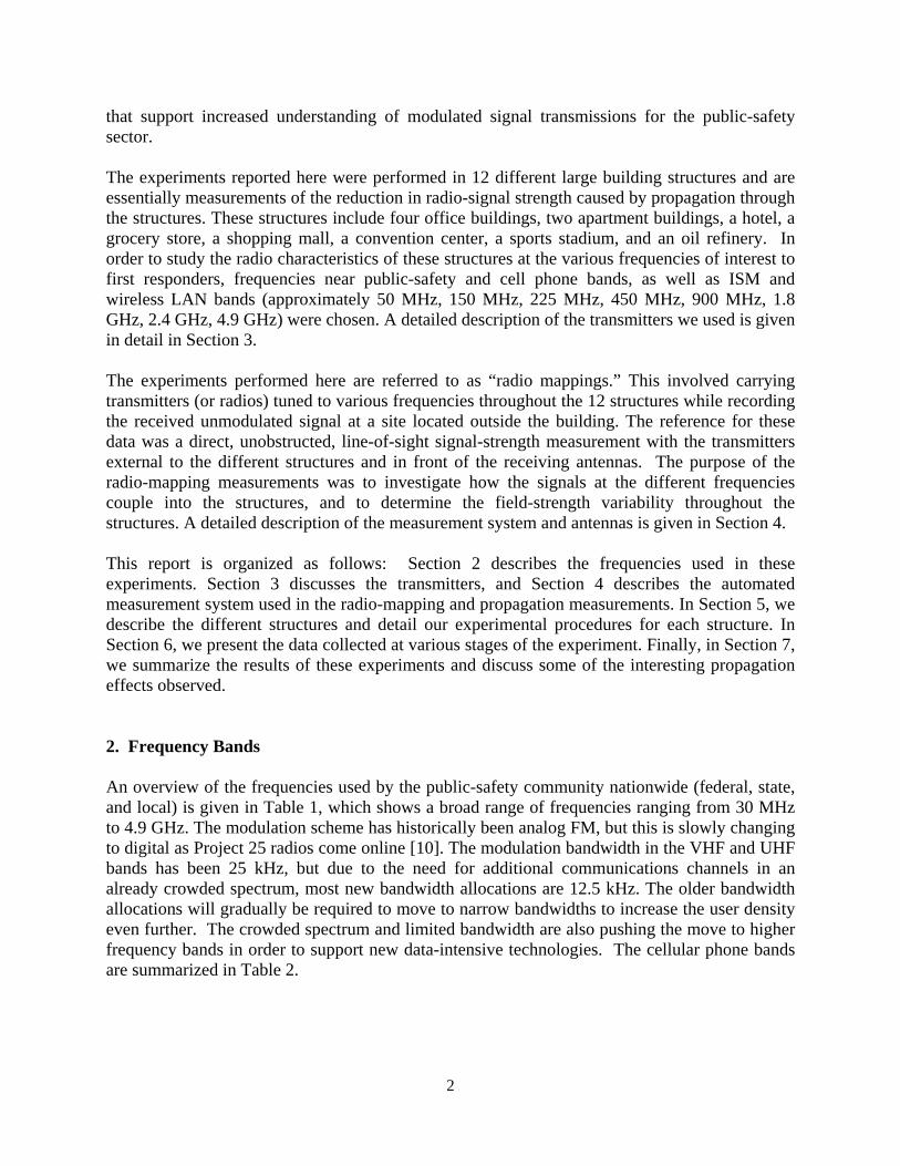
6.4 Colorado Springs, CO, CO Hotel Complex Results

The Colorado Springs, CO measurements consisted of a walk-through with a vertically polarized receive antenna, and a walk-through with a horizontally polarized receive antenna. Data were collected at two different receive locations as described in Section 5.4. Six frequencies were measured at the Colorado Springs, CO hotel, and the data is presented in Figures 98 through 129. The highest frequency, 1830 MHz, did not provide meaningful statistics, as is evident by the walk-through plots in Figure 103, Figure 111, Figure 119, and Figure 127. Hence, no statistics are provided for the 1830 MHz case. Note that this indicates that at 1830 MHz, the building essentially attenuated the transmitted signal below the detection threshold of the spectrum analyzer. Figure 98 though Figure 103 show the walk-through results for a vertically polarized receiver at site 1, with the corresponding statistics for the five lowest frequencies displayed in Figure 104 and Figure 105. Frequencies of 162 MHz, 225 MHz, 449 MHz, and 902 MHz behave quite similarly, as is evident by both the walk-through and statistics figures. However, the 49 MHz case demonstrates an increase in the reference signal level of greater than 16 dB compared to those four frequencies. The site 1 horizontally polarized receive antenna results in Figure 106s through Figure 111, with corresponding statistics in Figure 112 and

Figure 113, show some differences when compared to the site 1 vertically polarized receiver results. The basic shape of the histogram now illustrates a normal distribution (instead of an exponential), and the standard deviation decreases by at least 6.5 dB for all five frequencies. The walk-through results at receive site 2 with a vertically polarized receive antenna for the six frequencies are shown in Figure 114 to Figure 119, with the corresponding statistics shown in Figure 120 and Figure 121. In comparison to the case for site 1, the most noticeable difference is a decrease of at least 7.5 dB in the standard deviation across all five frequencies. The shapes of the histograms approximate exponential distributions, which is consistent with the site 1 results. Figure 122 through Figure 127 show the results for a horizontally polarized receive antenna at site 2, with corresponding statistics results displayed in Figure 128 and Figure 129. In comparison with the results for site 1, the shapes of the histograms, except for the 49 MHz case,

20

are tending toward a normal distribution. Interestingly, the standard deviations for all five frequencies are within 1.1 dB for this polarization at site 2, which represents the smallest spread in standard deviation for all four polarization and locations combinations.

6.5 Boulder, CO Grocery Store Results

The walk-through results for six frequencies tested in the Boulder grocery store are provided in Figure 130 through Figure 135. Due to the openness of both the entrance and the floor space of the building, the walk-through plots depict a clear geometrical distance dependency between the transmitter and the receiver for all frequencies. For example, see the section in the figures where the transmitter was carried back and forth along the aisles. The histogram shapes appear to follow a normal distribution, and the data exhibit similar statistical values for all frequencies (see Figure 136 and Figure 137). The openness of the facility is most likely responsible for this fairly close agreement across all frequencies.

6.6 Gaithersburg, MD Office Building Results

Figure 138 through Figure 143 depict the walk-through data for the office building in Gaithersburg, MD. The corresponding statistics are shown in Figure 144 and Figure 145. An interesting observation is that while all the walk-through results show the same general trends, the case of 1830 MHz clearly shows the received signal falling into the noise region when the transmitter is in the basement. Also, the shape of the histograms for 226 and 448 MHz does not mimic those for the other four frequencies, which have a significant number of samples that are either near or below the noise floor.

6.7 Bethesda, MD Shopping Mall Results

The both the walk-through data and the statistics data are presented in Figures 146 through 161. Walk-through data for receive sites 1 and 2 are plotted in Figure 146 through Figure 151, and Figure 154 through Figure 159, respectively. The corresponding statistics plots for site 1 are shown in Figure 152 and Figure 153, while the statistics for site 2 are shown in Figure 160 and Figure 161. The results for site 1 are quite similar across all six frequencies, with the most noticeable difference occurring at 1830 MHz. At this frequency, the received signal is either below or near the noise floor for many of the samples. This shows up in the sharp rise in the CDF at approximately -34 dB for the 1830 MHz plot in Figure 151. The first five frequencies do not exhibit this step-function-like behavior. At the second receiver site, the walk-through data again show very similar general behavior, such as the clear peaks when there is a line-of-sight at the Sears location. Also, the same step-function-like behavior shows up in the CDF of the 1830 MHz results.

21

6.8 Silver Springs, MD Office Building Results

Figure 162 to Figure 167 show the walk-through data for the Silver Springs office building. The number/letter pairs refer to a floor and location, see Figure 29. Note that the transmitters were carried into the lobby, transported by the elevator to the ninth floor, carried through several floors, into the basement, and then finally back to the lobby. The corresponding statistics plots are presented in Figure 168 and Figure 169. As in the shopping mall discussed above, the CDF of the 1830 MHz case resembles a step function. The standard deviation is approximately half the value compared to the other frequencies, as well.

6.9 Washington, DC Convention Center Results

Three receiver sites collected data at the Washington, DC convention center. The both the walk-through data and the statistics data for all three sites are presented in Figures 170 through 193. The corresponding walk-through data results for receiver sites labeled 1, 2, and 3 are provided in Figure 170 through Figure 175, Figure 178 through Figure 183, and Figure 186 through Figure 191, respectively. The statistics plots for receiver sites 1, 2, and 3 are found in Figure 176 and Figure 177, Figure 184 and Figure 185, and Figure 192 and Figure 193, respectively. The walk-through data plots depict very similar behavior for all frequencies at the three receiving sites. At 162 MHz, the standard deviation spread between sites is 3.2 dB, which is the maximum spread. It is interesting to note that the 1.8 GHz band demonstrates the lowest average standard deviation (approximately 11.8 dB), which is consistent with the rapid rise on the slope of the empirical CDFs. We also performed measurements before, during, and after the implosion of this structure, and details of these implosion measurements are reported in Reference [8]. 6.10 Boulder, CO Apartment Building Results

Two receive sites were used to collected data at the Boulder apartment building. The walk-through results for site 1 are shown in Figure 194 through 200, with the statistics plots provided in Figure 201 through 203. Site 2 results are shown in Figure 204 through 210, with the corresponding statistics plotted in Figure 211 through 213.

6.11 Commerce City, CO Oil Refinery Results The oil refinery results from a walk-through of the plant come from two receive sites, north and south. The both the walk-through data and the statistics data for both receive sites are presented in Figures 214 through 235. Figure 214 through Figure 221 represent the south site data while Figure 225 through Figure 232 show the north site data. The corresponding statistics data plots are Figure 222 to Figure 224, and Figure 233 to Figure 235, respectively.

22

Comparison between the collected data for the walk-through reveals that the median and mean for south site are in general lower than for the north site. The standard deviations are quite similar; the greatest difference (3.4 dB) occurs at 50 MHz. Examination of the individual walk-through data plot shows that position 4 creates the strongest signal at the south receive site. The top of the tower location presents a much stronger relative signal at the north site than at the south site. Data at the oil refinery were also collected along a road located among the large storage tanks. The collected data at the north site only are shown in Figure 236 through Figure 243, with the corresponding statistics plots provided in Figure 244 to Figure 246.

6.12 NIST Boulder, CO Laboratory Results Building 1 (or the Radio Building) at the NIST laboratory in Boulder, CO represents the final data collection site. One receiver site was located at the end of Wing 4 of the building (site 1), but still within the building structure. The second receiver location (site 2) was located outside off of Wing 6. Note that the data for site 1 contain only the walk-throughs to point D, or the farthest point, but not the return walk-through data. The both the walk-through data and the statistics data for both receive sites are presented in Figures 247 through 268. Figure 247 through Figure 254 and Figure 258 through Figure 265 show the walk-through plots for receiver sites 1 and 2, respectively. The corresponding statistics plots are provided in Figure 255 and Figure 257, and Figure 266 and Figure 268, respectively. The most significant difference between the two results shows up in the standard deviation. Across all frequencies, results for site 1 indicate a deviation at least 7.4 dB greater than results for site 2. This discrepancy is possible due to the close proximity of the path taken to receive site 1 during the walk-through, which created a much larger dynamic range for receive site 1 than for site 2. The discrepancy can also be due to the tunnel effect for the receiver inside the building, while the outside site had standard building penetration rather than waveguide below cutoff behavior. 7. Summary of Results and Conclusions The following tables, Tables 17 through 28, present summaries of the processed data by frequency bands. This enables easier comparisons between results from different building or structure types. (Note that the exact frequencies are provided in each of the individual site discussions.) Table entries include a building or structure identifier, the actual frequency tested, the specific reference level used to normalize that particular data set, and then median, mean, and standard deviation results for the normalized data.

23

Table 17. 50 MHz frequency band.

Structure/Location Freq.

(MHz)

Ref. level

(dBm) Median

(dB) Mean (dB)

Std. Dev. (dB)

New Orleans, LA apartment 50 3.7 35.9 37.5 13.1 Philadelphia, PA sports stadium

First inside walk; horiz. polar. 50 0.0 34.0 29.5 15.5 Second inside walk; horiz. polar. 50 0.0 44.4 42.8 8.8

Inside walk; vert. polar. 50 0.0 36.8 32.8 14.2 Outside walk; horiz. polar. 50 0.0 32.8 27.8 15.5 Outside walk; vert. polar. 50 0.0 41.8 36.0 18.4

Phoenix, AZ office Colorado Springs, CO, CO hotel

complex First walk-through, Receive site 1 50 23.7 62.8 58.0 17.6

Second walk-through, Receive site 1 50 29.2 58.2 56.2 11.1 First walk-through, Receive site 2 50 57.6 14.9 12.3 5.3

Second walk-through, Receive site 2 50 31.5 62.9 57.8 12.4 Grocery Store (Boulder, CO) 50 35.4 45.1 43.1 12.0

NIST office (Gaithersburg, MD) 50 21.3 68.6 62.1 16.5 Shopping mall (Bethesda, MD)

Receiver site 1 50 47.3 49.4 47.2 5.9 Receiver site 2 50 48.9 44.4 42.2 9.7

Discovery office (Silver Spring, MD) 50 21.6 64.2 63.7 11.4

Washington, DC convention center Receiver site 1 50 19.1 63.9 62.3 12.5 Receiver site 2 50 26.3 50.6 49.8 14.4 Receiver site 3 50 13.3 67.4 65.3 15.5

Horizon West Apartment (Boulder) Receiver site 1 Receiver site 2

Oil refinery (Commerce City, CO) Walk-through, south receive site 50 30.2 57.1 55.9 13.2 Walk-through, north receive site 50 25.6 52.6 50.3 16.6

Road drive, north receive site 50 27.5 51.9 51.2 7.3 NIST laboratory (Boulder, CO)


24



(MHz)

Ref. level

(dBm) Median

(dB) Mean (dB)

Std. Dev. (dB)




Phoenix, AZ office 154 12.8 62.3 60.9 18.4 Colorado Springs, CO Hotel

Complex First walk-through, Receive site 1 162 43.9 39.5 37.6 15.5


Second walk-through, Receive site 2 162 32.8 48.2 46.6 11.8 Grocery store (Boulder, CO) 162 36.5 38.6 36.0 11.8



Discovery office (Silver Spring, MD) 162 30.9 57.9 55.7 10.3 Washington, DC convention center

Receiver site 1 162 26.3 61.9 59.9 12.1 Receiver site 2 162 21.3 65.0 61.1 15.3 Receiver site 3 162 16.9 68.9 66.0 14.4

Horizon West apartment (Boulder, CO)





25



(MHz)

Ref. level

(dBm) Median

(dB) Mean (dB)

Std. Dev. (dB)

















26



(MHz)

Ref. level

(dBm) Median

(dB) Mean (dB)

Std. Dev. (dB)

















27



(MHz)

Ref. level

(dBm) Median

(dB) Mean (dB)

Std. Dev. (dB)




Phoenix, AZ office 867 34.4 38.3 37.9 13.5 Colorado Springs, CO, CO hotel






Discovery office (Silver Spring, MD) 902 16.0 72.1 70.4 10.5 Washington, DC convention center

Receiver site 1 902 16.5 63.8 61.8 14.5 Receiver site 2 902 23.5 55.4 54.0 13.7 Receiver site 3 902 9.4 68.5 66.4 14.1






28

Table 22. 1.8 GHz frequency band.

Structure/Location Freq. (GHz)

Ref. level

(dBm) Median

(dB) Mean (dB)

Std. Dev. (dB)

New Orleans, LA apartment 1.83 15.8 37.0 34.0 13.1 Philadelphia, PA sports stadium

First inside walk; horiz. polar. 1.83 0.0 44.9 40.4 14.3 Second inside walk; horiz. polar. 1.83 0.0 22.0 20.9 8.4

Inside walk; vert. polar. 1.83 0.0 26.9 26.5 9.5 Outside walk; horiz. polar. 1.83 0.0 45.6 39.4 17.1 Outside walk; vert. polar. 1.83 0.0 49.5 42.8 19.6


complex First walk-through, Receive site 1

Second walk-through, Receive site 1 First walk-through, Receive site 2

Second walk-through, Receive site 2 Grocery store (Boulder, CO) 1.83 34.2 40.8 39.3 12.0

NIST office (Gaithersburg, MD) 1.83 30.6 59.9 55.6 12.2 Shopping mall (Bethesda, MD)

Receiver site 1 1.83 62.2 34.1 33.3 3.9 Receiver site 2 1.83 55.0 41.0 37.7 8.5

Discovery office (Silver Spring, MD) 1.83 25.9 69.5 67.2 5.7 Washington, DC convention center

Receiver site 1 1.83 27.5 60.8 57.9 11.4 Receiver site 2 1.83 25.5 60.1 58.0 11.8 Receiver site 3 1.83 24.6 60.7 58.2 12.1



Oil refinery (Commerce City, CO) Walk-through, south receive site 1.83 31.2 50.3 49.4 12.3 Walk-through, north receive site 1.83 29.9 41.6 39.7 15.1

Road drive, north receive site 1.83 43.7 42.0 40.1 11.6 NIST laboratory (Boulder, CO)


29



Ref. level

(dBm) Median

(dB) Mean (dB)

Std. Dev. (dB)








Ref. level

(dBm) Median

(dB) Mean (dB)

Std. Dev. (dB)






The next two tables provide insight into some overall behavior trends. Table 25 lists the overall statistics computed on the standard deviation results from all the building measurements. For example, the second row contains the median values of the standard deviation computed for all the buildings across all the measured frequencies. The similar values of these overall statistics indicate that the standard deviation behaves in a very similar fashion across all the frequencies.

30

Table 25. Statistics of the standard deviation behavior for all the buildings.

Frequency Band:

50 MHz

150 MHz

225 MHz

450 MHz

900 MHz

1.8 GHz

2.4 GHz

4.9 GHz

Median 13.10 12.30 13.30 12.20 13.65 12.00 13.70 13.60

Mean 12.67 12.65 12.72 12.72 13.44 11.77 13.50 12.95

Maximum 18.40 19.20 20.30 20.70 22.30 19.60 17.50 16.80

Minimum 5.30 5.80 5.90 5.60 6.30 3.90 9.60 9.00

Std. Dev. 3.71 3.31 3.66 3.24 3.50 3.66 2.92 3.07

For a rough insight into the attenuation behavior, we examine mean values for eleven of the scenarios (see Table 26). Each scenario uses the receive site that typically provided the greatest dynamic range so as to reduce the impact of the limited dynamic range of the test equipment. Table 27 shows the mean values of the various frequencies for eleven scenarios listed in Table 26. Values in Table 27 were computed in decibels after subtracting the reference level. Note that the combination of the reference level and the dynamic limitations of the test equipment can skew the statistics. The approximate noise floor provides an approximate value for the useable dynamic range. To obtain a rough idea of how close the mean signal is to the noise floor, we compute the difference between the mean signal level and the noise floor. The results for the eleven scenarios are shown in Table 28. In general, a greater difference implies less impact on the statistical results due to measured values at or below the noise floor. For example, the results for scenario six indicate mean signal levels very near the approximate noise floor, as indicated by a difference of less than 10 dB for all the frequencies. In contrast, scenario 10 indicates at least a 23 dB separation between the mean signal level and the noise floor for all frequencies.

Table 26. Test scenarios used in examination of structure/building shielding.

Selected test scenarios

1. New Orleans, LA apartment 2. Philadelphia, PA sports stadium: inside walk; vertical polarization 3. Colorado Springs, CO, CO hotel complex: first walk-through; receive site 1 4. Grocery store, Boulder, CO 5. NIST office, Gaithersburg, MD 6. Shopping mall, Bethesda, MD: receive site 1 7. Discovery office, Silver Spring, MD 8. Washington, DC convention center: receive site 3 9. Horizon West apartment, Boulder, CO: receive site 1 10. Oil refinery, Commerce City, CO: walk-through, north receive site 11. NIST laboratory, Boulder, CO: receive site 1

31

Table 27. Mean values of scenarios used for structure/building attenuation statistics.

Scenario

50 MHz

150 MHz

225 MHz

450 MHz

900 MHz

1.8 GHz

2.4 GHz 4.9 GHz

1 37.5 27.9 33.1 39.7 34.2 34.0 NA NA 2 32.8 39.2 34.2 28.7 27.2 26.5 NA NA 3 58.0 37.6 39.5 30.0 34.1 NA NA NA 4 43.1 36.0 43.0 29.2 33.8 39.3 NA NA 5 62.1 41.6 44.1 46.9 57.7 55.6 NA NA 6 47.2 46.5 49.9 52.8 44.6 33.3 NA NA 7 63.7 55.7 60.3 52.4 70.4 67.2 NA NA

8 65.3 66.0 62.3 57.3 66.4 58.2 NA NA

9 NA 24.9 25.9 25.4 27.0 25.6 17.5 36.3 10 50.3 33.7 34.1 37.8 42.7 39.7 41.1 48.5 11 50.2 54.8 43.3 37.9 28.9 26 62.7 59.9

Table 28. Difference in dB between the mean signal level and the noise floor for the scenarios used in the structure/building attenuation statistics.

Scenario

50 MHz

150 MHz

225 MHz

450 MHz

900 MHz

1.8 GHz

2.4 GHz 4.9 GHz

1 21.5 19.1 17.9 12.3 30.8 16.0 NA NA 2 16.2 33.8 25.8 27.3 24.8 13.5 NA NA 3 18.0 18.4 19.5 24.0 21.9 NA NA NA 4 22.9 28.0 25.0 36.8 36.2 23.7 NA NA 5 15.9 16.4 24.9 23.1 19.3 10.4 NA NA 6 4.8 3.5 8.1 3.2 4.4 1.7 NA NA 7 14.3 11.3 17.7 17.6 12.6 3.8 NA NA 8 20.7 18.0 29.7 27.7 22.6 13.8 NA NA 9 NA 66.1 69.1 67.6 57.0 48.4 27.5 8.5

10 23.7 45.3 46.9 42.2 34.3 33.3 36.9 24.5 11 16.8 33.2 24.7 28.1 35.1 19.0 20.3 20.1

Differences in building types make it difficult to provide clear general statements based on the collected data. However, we can observe some general trends.

32

First, examination of the standard deviation yields some interesting insights. In particular, if we exclude the first receiver site for the NIST laboratory in Boulder, CO, we see that the average standard deviation for the six lower frequency bands ranges from 11.8 dB to 13.4 dB. Limited data were collected for the upper two frequencies; but if we include those results, the upper limit of the range increases to 14.9 dB. Across all frequency bands, the range of maximum standard deviation covers 16.8 dB to 22.3 dB, with 22.3 dB occurring at 900 MHz. The minimum standard deviation values range from 3.9 dB to 12.1 dB, with 3.9 dB occurring at 1.8 GHz. Second, in almost all cases, the median value for the power received is less than the average power received. The typical difference is between 2 dB to 3 dB. This suggests that median value may be a better measure for representing the general behavior of the building, or at least a more conservative performance measure. Third, the histograms (which approximate PDFs) and the empirical CDFs appear to follow no typical density function. To some extent, each individual test case will generate a unique density. However, the data seem not to suggest any obvious average or best approximation density that could be used as a collective representation of the buildings. The data presented in this report aid in understanding the issues faced with first responders communicating into and within large building structures. For example, the large amount of attenuation for the signals coupling into the different structures indicates to system designers what a communication link must overcome in order to have a reliable system. In addition, the measured signal variability indicates the dynamic environment these different buildings present to a communication system. The results in this report are the fourth in a series of reports detailing experiments performed by NIST in order to better understand the first responder radio propagation environment. The first three reports cover implosion experiments performed in three different building structures, an apartment building in New Orleans, LA, a large sports stadium (the “Veterans Stadium”) in Philadelphia, PA, and a convention center in Washington, DC. Other experiments at different frequencies in other building structures are being performed and will published separately. We are also performing measurement to simulate and test the performance of ad-hoc networks in various building structures, and the results of these experiments will also be published separately.

—————————

Disclaimer: Mention of any company names serves only for identification, and does not constitute or imply NIST endorsement of such a company or of its products.

—————————

This work was sponsored by the U.S. Department of Justice and the U.S. Department of Homeland Security through the Office of Law Enforcement Standards of NIST. We thank

33

members of the technical staff of the Electromagnetics Division 818, who pulled together the equipment, and Dennis Friday, Perry Wilson, and Mike Kelley for managerial support. Finally, we thank the companies, owners, and individuals who allowed us access to the building structures and for help during these experiments.

34

8. References [1] Statement of Requirements: Background on Public Safety Wireless Communications,

The SAFECOM Program, Department of Homeland Security, Vol. 1, March 10, 2004. [2] M. Worrell and A. MacFarlane, Phoenix Fire Department Radio System Safety Project,

Phoenix Fire Dept. Final Report, October 8, 2004, http://www.ci.phoenix.az.us/FIRE/radioreport.pdf.

[3] 9/11 Commission Report, National Commission on Terrorist Attacks upon the United

States, 2004. [4] Final Report for September 11, 2001 New York World Trade Center terrorist attack,

Wireless Emergency Response Team (WERT), October 2001. [5] C.L. Holloway, G. Koepke, D. Camell, K.A. Remley, D.F. Williams, S. Schima, S.

Canales, and D.T. Tamura, “Propagation and Detection of Radio Signals Before, During and After the Implosion of a Thirteen Story Apartment Building,” Natl. Inst. Stand. Technol., Technical Note 1540, May 2005.

[6] C.L. Holloway, G. Koepke, D. Camell, K.A. Remley, and D.F. Williams, “Radio

Propagation Measurements During a Building Collapse: Applications for First Responders,” Proc. Intl. Symp. Advanced Radio Tech., pp. 61-63, March 2005.

[7] C.L. Holloway, G. Koepke, D. Camell, K.A. Remley, D.F. Williams, S. Schima, and

D.T. Tamura, “Propagation and Detection of Radio Signals Before, During and After the Implosion of a Large Sports Stadium (Veterans Stadium in Philadelphia),” Natl. Inst. Stand. Technol., Technical Note 1541, October 2005.

[8] C.L. Holloway, G. Koepke, D. Camell, K.A. Remley, D.F. Williams, S. Schima, M.

McKinely, and R.T. Johnk, “Propagation and Detection of Radio Signals Before, During and After the Implosion of a Large Convention Center,” Natl. Inst. Stand. Technol., Technical Note 1542, June 2006.

[9] K.A. Remley, G. Koepke, C.L. Holloway, C. Grosvenor, D. Camell, J. Ladbury, D.

Novotny, W.F. Young, M.D. McKinley, Y. Becquet, and J. Korsnes, “Propagation and Detection of Radio Signals Before, During and After the Implosion of a Large Convention Center,” Natl. Inst. Stand. Technol., Technical Note 1546, December 2007.

[10] APCO International, APCO Project 25 Standards for Public Safety Digital Radio, August

1995, http://www.apcointl.org/frequency/project25/information.html#documents.

35

9. Figures

Figure 1. Typical transmitters used for the four lower frequency bands.

Figure 2. Transmitters used for the higher frequency bands.

36

Figure 3. Schematic of the receiving system for the building penetration and field-mapping experiments.

WidebandPower

Combiner

50 MHzVertical Whip

1830 MHzYagi Antenna

900 MHzYagi Antenna

120 - 1000 MHzLPDA

Portable Spectrum Analyzer

Antenna Mast installed inTRIPOD or CART

GPS Receiver

37

Figure 4. Antennas mounted on a tripod.

Figure 5. Antennas mounted on the mobile cart.

38

Figure 6. The New Orleans, LA Fisher apartment building.

39

Figure 7. Inside the New Orleans, LA apartment building.

40

Figure 8. Receiver location and layout for the New Orleans, LA apartment building experiments.

NIST receiving site

Apartment Building

41

Figure 9. The Veterans Stadium in Philadelphia, PA.

42

Figure 10. Inside the Veterans Stadium.

43

Figure 11. Receiver location and layout for the stadium experiments.

44

Figure 12. The office building in Phoenix, AZ.

45

Figure 13. Inside the office building in Phoenix, AZ.

46

Figure 14. Receiver location and layout for the Phoenix, AZ office building.

NIST receiving site

47

Figure 15. The hotel complex in Colorado Springs, CO, CO.

48

Figure 16. Inside the hotel complex in Colorado Springs, CO, CO.

49

Figure 17. Receiver location and layout for the Colorado Springs, CO hotel complex.

50

Figure 18. The grocery store in Boulder, CO.

51

Figure 19. Inside the grocery store in Boulder, CO.

52

.

Figure 20. Receiver location and layout for the Boulder, CO grocery store.

53

Figure 21. The NIST office building in Gaithersburg, MD.

54

Figure 22. Receiver location and layout for the NIST Gaithersburg, MD office building.

55

Figure 23. The shopping mall in Bethesda, MD.

56

Figure 24. Inside the shopping mall in Bethesda, MD.

57

Figure 25. Receiver location and layout for the Bethesda, MD shopping mall.

NIST receiving site 2 NIST receiving site 1

58

Figure 26. Upper and lower level floor plan with the predetermined locations on both levels of the shopping mall. The green arrows in the figure represent the actual paths that were walked.

2

3

4

5

6

7

1

8 9

10

11

12 13

Start

14

1917

15

16 20 21

23

22

18

24

25 Return to

59

Figure 27. The Discovery office building in Silver Springs, MD.

60

Figure 28. Inside the Discovery office building in Silver Springs, MD.

61

Figure 29: Building layout and measurement locations for the Discovery building.

62

Figure 30. Receiver location and layout for the Discovery office building in Silver Springs, MD.

Receiving site

63

Figure 31. The convention center in Washington, DC.

64

Figure 32. Inside the convention center in Washington, DC.

65

Figure 33. Receiver location and layout for the convention center in Washington, DC.

Three NIST receiving sites

66

Figure 34. Horizon West apartment building in Boulder, CO.

67

Figure 35. Transmitter locations for Horizon West.

68

Figure 36. Receiver setups for Horizon West apartment building in Boulder, CO.

69

Figure 37. Inside the Horizon West apartment building in Boulder, CO.

70

Figure 38. Overview of the Inside the SUNCOR oil refinery in Commerce City, CO.

71

Figure 39. The receiver locations at the SUNCOR oil refinery in Commerce City, CO.

72

Figure 40. Inside the SUNCOR oil refinery in Commerce City, CO.

73

Figure 41. The driven section of the data collection process at the SUNCOR oil refinery.

74

Figure 42. Receiver location and layout for the Commerce City, CO oil refinery.

NIST North Site

NIST South Site

1

11

10

2

3

4

6

7

8

9

12

5

NIST North Site

NIST South Site

11

1111

1010

22

33

44

66

77

88

99

1212

55

75

Figure 43. NIST main building (the Radio Building) in Boulder, CO.

76

Figure 44. The receiver setups for the NIST’s laboratories in Boulder, CO.

77

Figure 45. Receiver location and layout for the Boulder, CO laboratories.

C

BWing 6 receive site

A

D

Wing 4 receive siteReference Location

78

Figure 46. New Orleans, LA apartment building walk-through at 49.60 MHz.


50 100 150 200 250 300 350 400 450 500 550-80

-70

-60

-50

-40

-30

-20

-10

0

10

20

sample number

Pow

er (

dB)

Freq. = 49 MHzRef. = -3.7 dBmApprox. noise fl. = -59 dB

Floor 1

Floor 12

Floor 1

window

FL 2

window

FL 4

window

FL 6

window

FL 8

window

FL 10

window

FL 12

room on the roof

Floor 12

Floor 2

outside

stairwell stairwellroof

50 100 150 200 250 300 350 400 450 500 550-70

-60

-50

-40

-30

-20

-10

0

10

20

sample number

Pow

er (

dB)

Freq. = 162 MHz

Ref. = -2.5 dBm

Approx. noise fl. = -47 dB

Floor 1

Floor 12

Floor 1

window

FL

2

window

FL

4w

indow F

L 6

window

FL

8w

indow F

L 10

window

FL

12

room on the roof

Floor 12

Floor 2

outside

stairwell stairwell roof

79



50 100 150 200 250 300 350 400 450 500 550-70

-60

-50

-40

-30

-20

-10

0

10

20

sample number

Pow

er (

dB)

Freq. = 448 MHz

Ref. = -3.2 dBmApprox. noise fl. = -52 dB

Floor 1

Floor 12

Floor 1

window

FL

2

window

FL

4w

indow F

L 6

window

FL

8w

indow F

L 10

window

FL

12

room on the roof

FL 12

FL 2

outside

50 100 150 200 250 300 350 400 450 500 550-70

-60

-50

-40

-30

-20

-10

0

10

20

sample number

Pow

er (

dB)

Freq. = 448 MHz


Floor 1

Floor 12

Floor 1

window

FL

2

window

FL

4w

indow F

L 6

window

FL

8w

indow F

L 10

window

FL

12

room on the roof

Floor 12

Floor 2

outside


50 100 150 200 250 300 350 400 450 500 550-70

-60

-50

-40

-30

-20

-10

0

10

20

sample number

Pow

er (

dB)

Freq. = 225 MHz

Ref. = -9.3 dBm


Floor 1

Floor 12

Floor 1

window

FL

2

window

FL

4w

indow F

L 6

window

FL

8w

indow F

L 10

window

FL

12

room on the roof

Floor 12

Floor 2

outside


80

Figure 50. New Orleans, LA apartment building walk-through at 902.60 MHz


50 100 150 200 250 300 350 400 450 500 550-90

-80

-70

-60

-50

-40

-30

-20

-10

0

10

20

sample number

Pow

er (

dB)


Floor 1

Floor 12

Floor 1

window

FL

2

window

FL

4w

indow F

L 6

window

FL

8w

indow F

L 10

window

FL

12

room on the roof

Floor 12

Floor 2

outside


50 100 150 200 250 300 350 400 450 500 550

-70

-60

-50

-40

-30

-20

-10

0

10

20

sample number

Pow

er (

dB)


Floor 1

Floor 12

Floor 1

window

FL

2

window

FL

4w

indow F

L 6

window

FL

8w

indow F

L 10

window

FL

12

room on the roof

Floor 12

Floor 2

outside


81

Figure 52. New Orleans, LA apartment building statistics, histograms, and empirical CDF for walk-through data at 49.60, 162.00, and 225.375 MHz.

-70 -60 -50 -40 -30 -20 -10 0 100

10

20

30

40

50

freq. = 49 MHz

ref. = -3.7 dBm

median = -35.9 dB

mean = -37.5 dB

std. dev. = 13.1 dB

-70 -60 -50 -40 -30 -20 -10 0 100

0.2

0.4

0.6

0.8

1

-70 -60 -50 -40 -30 -20 -10 0 100

10

20

30

40

50

freq. = 162 MHz

ref. = -2.5 dBm

median = -28.2 dB

mean = -27.9 dB

std. dev. = 11.8 dB

-70 -60 -50 -40 -30 -20 -10 0 100

0.2

0.4

0.6

0.8

1

-70 -60 -50 -40 -30 -20 -10 0 100

10

20

30

40

50

freq. = 225 MHz

ref. = -9.3 dBm

median = -34.5 dB

mean = -33.1 dB

std. dev. = 11.2 dB

-70 -60 -50 -40 -30 -20 -10 0 100

0.2

0.4

0.6

0.8

1

Power (dB)

N

CD

F

82

Figure 53. New Orleans, LA apartment building statistics, histograms, and empirical CDF for walk-through data at 448.60, 902.60, and 1832.50 MHz.

-70 -60 -50 -40 -30 -20 -10 0 100

10

20

30

40

50

freq. = 448 MHz

ref. = -3.2 dBm

median = -42.6 dB

mean = -39.7 dB

std. dev. = 10.3 dB

-70 -60 -50 -40 -30 -20 -10 0 100

0.2

0.4

0.6

0.8

1

-70 -60 -50 -40 -30 -20 -10 0 100

10

20

30

40

50

freq. = 902 MHz

ref. = -1.0 dBm

median = -34.8 dB

mean = -34.2 dB

std. dev. = 13.8 dB

-70 -60 -50 -40 -30 -20 -10 0 100

0.2

0.4

0.6

0.8

1

-70 -60 -50 -40 -30 -20 -10 0 100

10

20

30

40

50

freq. = 1830 MHz

ref. = -15.8 dBm

median = -37.0 dB

mean = -34.0 dB

std. dev. = 13.1 dB

-70 -60 -50 -40 -30 -20 -10 0 100

0.2

0.4

0.6

0.8

1

Power (dB)

N

CD

F

83

Figure 54. Philadelphia, PA sports stadium first inside walk at 49.60 MHz; horizontal polarization.


20 40 60 80 100 120 140-70

-60

-50

-40

-30

-20

-10

0

10

20

sample number

Pow

er(

dB)

Freq. = 49 MHz

Ref. = 0.0 dBm


ramp into stadium

level 300

level 400

level 500

level 600

level 700

L700, col.10

level 700, col.100

level 700, col.85

level 700, col.75

level 700, col.65

level 700, col.45

level 700, col.35

level 700, col.25

level 700, col.15

20 40 60 80 100 120 140-80

-70

-60

-50

-40

-30

-20

-10

0

10

20

sample number

Pow

er (

dB)

Freq. = 162 MHzRef. = 0.0 dBmApprox. noise fl. = -71 dB

ramp into stadium

level 300

level 400

level 500

level 600

level 700

L700, col.10

level 700, col.100

level 700, col.85

level 700, col.75

level 700, col.65

level 700, col.45

level 700, col.35

level 700, col.25

level 700, col.15

84



20 40 60 80 100 120 140-80

-70

-60

-50

-40

-30

-20

-10

0

10

20

sample number

Pow

er (

dB)


ramp into stad.

level 300

level 400

level 500

level 600

level 700

L700, col.10

L700, col.100

level 700, col.85

level 700, col.75

level 700, col.65

level 700, col.45

level 700, col.35

level 700, col.25

level 700, col.15

20 40 60 80 100 120 140-80

-70

-60

-50

-40

-30

-20

-10

0

10

20

sample number

Pow

er (

dB)


ramp into stadium

level 300

level 400

level 500

level 600

level 700

level 700, col.10

level 700, col.100

level 700, col.85

level 700, col.75

level 700, col.65

level 700, col.45

level 700, col.35

level 700, col.25

level 700, col.15

85


Figure 59. Philadelphia sports stadium first inside walk at 1832.00 MHz; horizontal polarization.

20 40 60 80 100 120 140-80

-70

-60

-50

-40

-30

-20

-10

0

10

20

sample number

Pow

er (

dB)


ramp into stadium

level 300

level 400

level 500

level 600

level 700

L700, col.10

level 700, col.100

level 700, col.85

level 700, col.75

level 700, col.65

level 700, col.45

level 700, col.35

level 700, col.25

level 700, col.15

20 40 60 80 100 120 140-80

-70

-60

-50

-40

-30

-20

-10

0

10

20

sample number

Pow

er (

dB)


ramp into stadium

level 300

level 400

level 500

level 600

level 700

level 700, col.10

level 700, col.100

level 700, col.85

level 700, col.75

level 700, col.65

level 700, col.45

level 700, col.35

level 700, col.25

level 700, col.15

Ref. = 0.0 dBm

86

Figure 60. Philadelphia, PA sports stadium statistics, histograms, and empirical CDF for first inside walk data at 49.60, 162.09, and 225.30 MHz; horizontal polarization.

-70 -60 -50 -40 -30 -20 -10 0 100

4

8

12

16

20

freq. = 49 MHz

ref. = 0.0 dBm

median = -34.0 dB

mean = -29.5 dB

std. dev. = 15.5 dB

-70 -60 -50 -40 -30 -20 -10 0 100

0.2

0.4

0.6

0.8

1

-70 -60 -50 -40 -30 -20 -10 0 100

4

8

12

16

20

freq. = 162 MHz

ref. = 0.0 dBm

median = -37.4 dB

mean = -34.2 dB

std. dev. = 15.0 dB

-70 -60 -50 -40 -30 -20 -10 0 100

0.2

0.4

0.6

0.8

1

-70 -60 -50 -40 -30 -20 -10 0 100

4

8

12

16

20

freq. = 225 MHz

ref. = 0.0 dBm

median = -34.4 dB

mean = -29.1 dB

std. dev. = 14.4 dB

-70 -60 -50 -40 -30 -20 -10 0 100

0.2

0.4

0.6

0.8

1

Power (dB)

N

CD

F

87

Figure 61. Philadelphia, PA sports stadium statistics, histograms, and empirical CDF for First inside walk data at 448.50, 902.45, and 1832.00 MHz; horizontal polarization.

-70 -60 -50 -40 -30 -20 -10 0 100

4

8

12

16

20

freq. = 448 MHz

ref. = 0.0 dBm

median = -35.9 dB

mean = -32.4 dB

std. dev. = 15.1 dB

-70 -60 -50 -40 -30 -20 -10 0 100

0.2

0.4

0.6

0.8

1

-70 -60 -50 -40 -30 -20 -10 0 100

4

8

12

16

20

freq. = 902 MHz

ref. = 0.0 dBm

median = -40.7 dB

mean = -35.8 dB

std. dev. = 15.3 dB

-70 -60 -50 -40 -30 -20 -10 0 100

0.2

0.4

0.6

0.8

1

-70 -60 -50 -40 -30 -20 -10 0 100

4

8

12

16

20

freq. = 1830 MHz

ref. = -1.6 dBm

median = -44.9 dB

mean = -40.4 dB

std. dev. = 14.3 dB

-70 -60 -50 -40 -30 -20 -10 0 100

0.2

0.4

0.6

0.8

1

Power (dB)

N

CD

F

ref = 0.0 dBm

88

Figure 62. Philadelphia, PA sports stadium second inside walk at 49.60 MHz; horizontal polarization.


50 100 150 200 250 300 350 400-70

-60

-50

-40

-30

-20

-10

0

10

20

sample number

Pow

er (

dB)

Freq. = 49 MHz

Ref. = 0.0 dBm


level 100, col.8

level 100, col.3

level 100, col.100

level 100, col.87

moving to field

field, col.80

field, col.55

field, col.10

moving from

field to level 100level 100, col.25

level 100, col.31

level 100, col.30

center of the fieldleaving center of the field

out of the stadium

50 100 150 200 250 300 350 400-80

-70

-60

-50

-40

-30

-20

-10

0

10

20

sam ple num ber

Pow

er (

dB)

F req . = 162 M H zR ef. = 0 .0 dB mA pprox. noise fl. = -63 dB

level 100, col.8

level 100, col.3

level 100, col.100

level 100, col.87

moving to field

field, col.80

field, col.55

field, col.10

moving from

field to L100

level 100, col.25

level 100, col.31

level 100, col.30

center of the field

leaving center of the field

out of the stadium

89



50 100 150 200 250 300 350 400-80

-70

-60

-50

-40

-30

-20

-10

0

10

20

sample number

Pow

er (

dB)


level 100, col.8

level 100, col.3

level 100, col.100

level 100, col.87

moving to field

field, col.80

field, col.55

field, col.10

moving from

field to L100

level 100, col.25

level 100, col.31

level 100, col.30


out of the stadium

50 100 150 200 250 300 350 400-80

-70

-60

-50

-40

-30

-20

-10

0

10

20

sample number

Pow

er (

dB)


level 100, col.8

level 100, col.3

level 100, col.100

level 100, col.87

moving to field

field, col.80

field, col.55

field, col.10

moving from

field to L100

level 100, col.25

level 100, col.31

level 100, col.30


out of the stadium

90



50 100 150 200 250 300 350 400 450-90

-80

-70

-60

-50

-40

-30

-20

-10

0

10

20

sample number

Pow

er (

dB)


level 100, col.8

level 100, col.3

level 100, col.100

level 100, col.87

moving to field

field, col.80

field, col.55

field, col.10

moving from

field to level 100level 100, col.25

level 100, col.31

level 100, col.30


out of the stadium

50 100 150 200 250 300 350 400 450-50

-40

-30

-20

-10

0

10

20

sam ple num ber

Pow

er (

dB)

F req. = 1830 M Hz

R ef. = 0.0 dBm

A pprox. noise fl. = -30 dB

level 100, col.8

level 100, col.3

level 100, col.100

level 100, col.87

moving to field

field, col.80

field, col.55

field, col.10

moving from

field to L100

level 100, col.25

level 100, col.31

level 100, col.30


out of the stadium

91

Figure 68. Philadelphia, PA sports stadium statistics, histograms, and empirical CDF for second inside walk data at 49.60, 162.09, and 225.30 MHz; horizontal polarization.

Power (dB)

N

CD

F

-80 -70 -60 -50 -40 -30 -20 -10 0 100

10

20

30

40

50

freq. = 49 MHz

ref. = 0.0 dBm

median = -44.4 dB

mean = -42.8 dB

std. dev. = 8.8 dB

-80 -70 -60 -50 -40 -30 -20 -10 0 100

0.2

0.4

0.6

0.8

1

-80 -70 -60 -50 -40 -30 -20 -10 0 100

10

20

30

40

50

freq. = 162 MHz

ref. = 0.0 dBm

median = -34.3 dB

mean = -35.6 dB

std. dev. = 10.6 dB

-80 -70 -60 -50 -40 -30 -20 -10 0 100

0.2

0.4

0.6

0.8

1

-80 -70 -60 -50 -40 -30 -20 -10 0 100

10

20

30

40

50

freq. = 225 MHz

ref. = 0.0 dBm

median = -37.6 dB

mean = -38.9 dB

std. dev. = 9.6 dB

-80 -70 -60 -50 -40 -30 -20 -10 0 100

0.2

0.4

0.6

0.8

1

92

Figure 69. Philadelphia, PA sports stadium statistics, histograms, and empirical CDF for second inside walk data at 448.50, 902.45, and 1832.00 MHz; horizontal polarization.

-80 -70 -60 -50 -40 -30 -20 -10 0 100

10

20

30

40

50

freq. = 448 MHz

ref. = 0.0 dBm

median = -35.7 dB

mean = -35.9 dB

std. dev. = 8.9 dB

-80 -70 -60 -50 -40 -30 -20 -10 0 100

0.2

0.4

0.6

0.8

1

-80 -70 -60 -50 -40 -30 -20 -10 0 100

10

20

30

40

50

freq. = 902 MHz

ref. = 0.0 dBm

median = -49.8 dB

mean = -50.2 dB

std. dev. = 15.8 dB

-80 -70 -60 -50 -40 -30 -20 -10 0 100

0.2

0.4

0.6

0.8

1

-80 -70 -60 -50 -40 -30 -20 -10 0 100

15

30

45

60

75

freq. = 1830 MHzref. = 0.0 dBm

median = -22.0 dBmean = -20.9 dBstd. dev. = 8.4 dB

-80 -70 -60 -50 -40 -30 -20 -10 0 100

0.2

0.4

0.6

0.8

1

Power (dB)

N

CD

F

93

Figure 70. Philadelphia, PA sports stadium inside walk at 49.60 MHz; vertical polarization.


50 100 150 200 250 300-70

-60

-50

-40

-30

-20

-10

0

10

20

sample number

Pow

er (

dB)

Freq. = 49 MHz

Ref. = 0.0 dBm


level 700, col.20

level 700, col.65

level 700, col.104

level 600

level 300

level 100

field, col.65

field, col.35

field, col.98

level 100, col.75

level 100, col.90

col.8

50 100 150 200 250 300-90

-80

-70

-60

-50

-40

-30

-20

-10

0

10

20

sample number

Pow

er (

dB)


level 700, col.20

level 700, col.65

level 700, col.104

level 600

level 300

level 100

field, col.65

field, col.35

field, col.98

level 100, col.75

level 100, col.90

col.8

94



50 100 150 200 250 300-80

-70

-60

-50

-40

-30

-20

-10

0

10

20

sample number

Pow

er (

dB)


level 700, col.20

level 700, col.65

level 700, col.104

level 600

level 300

level 100

field, col.65

field, col.35

field, col.98

level 100, col.75

level 100, col.90

col.8

50 100 150 200 250 300-80

-70

-60

-50

-40

-30

-20

-10

0

10

20

sample number

Pow

er (

dB)


level 700, col.20

level 700, col.65

level 700, col.104

level 600

level 300

level 100

field, col.65

field, col.35

field, col.98

level 100, col.75

level 100, col.90

col.8

95



50 100 150 200 250 300-70

-60

-50

-40

-30

-20

-10

0

10

20

sample number

Pow

er (

dB)

Freq. = 902 MHz

Ref. = 0.0 dBm


level 700, col.20

level 700, col.65

level 700, col.104

level 600

level 300

level 100

field, col.65

field, col.35

field, col.98

level 100, col.75

level 100, col.90

col.8

50 100 150 200 250 300-60

-50

-40

-30

-20

-10

0

10

20

sample number

Pow

er (

dB)

Freq. = 1830 MHz

Ref. = 0.0 dBm


level 700, col.20

level 700, col.65

level 700, col.104

level 600

level 300

level 100

field, col.65

field, col.35

field, col.98

level 100, col.75

level 100, col.90

col.8

96

Figure 76. Philadelphia, PA sports stadium statistics, histograms, and empirical CDF for inside walk data at 49.60, 162.09, and 225.30 MHz; vertical polarization.

-80 -70 -60 -50 -40 -30 -20 -10 0 100

5

10

15

20

25

freq. = 49 MHzref. = 0.0 dBm


-80 -70 -60 -50 -40 -30 -20 -10 0 100

0.2

0.4

0.6

0.8

1

-80 -70 -60 -50 -40 -30 -20 -10 0 100

4

8

12

16

20

freq. = 162 MHz

ref. = 0.0 dBm

median = -42.5 dB

mean = -39.2 dB

std. dev. = 15.8 dB

-80 -70 -60 -50 -40 -30 -20 -10 0 100

0.2

0.4

0.6

0.8

1

-80 -70 -60 -50 -40 -30 -20 -10 0 100

4

8

12

16

20

freq. = 225 MHz

ref. = 0.0 dBm

median = -36.3 dB

mean = -34.2 dB

std. dev. = 13.5 dB

-80 -70 -60 -50 -40 -30 -20 -10 0 100

0.2

0.4

0.6

0.8

1

Power (dB)

N

CD

F

97

Figure 77. Philadelphia, PA sports stadium statistics, histograms, and empirical CDF for inside walk data at 448.50, 902.45, and 1832.00 MHz; vertical polarization.

-80 -70 -60 -50 -40 -30 -20 -10 0 100

4

8

12

16

20

freq. = 448 MHz

ref. = 0.0 dBm

median = -29.8 dB

mean = -28.7 dB

std. dev. = 11.3 dB

-80 -70 -60 -50 -40 -30 -20 -10 0 100

0.2

0.4

0.6

0.8

1

-80 -70 -60 -50 -40 -30 -20 -10 0 100

4

8

12

16

20

freq. = 902 MHz

ref. = 0.0 dBm

median = -27.5 dB

mean = -27.2 dB

std. dev. = 11.3 dB

-80 -70 -60 -50 -40 -30 -20 -10 0 100

0.2

0.4

0.6

0.8

1

-80 -70 -60 -50 -40 -30 -20 -10 0 100

4

8

12

16

20

freq. = 1830 MHz

ref. = 0.0 dBm

median = -26.9 dB

mean = -26.5 dB

std. dev. = 9.5 dB

-80 -70 -60 -50 -40 -30 -20 -10 0 100

0.2

0.4

0.6

0.8

1

Power (dB)

N

CD

F

98

Figure 78. Philadelphia, PA sports stadium outside walk at 49.60 MHz; horizontal polarization.


10 20 30 40 50 60 70 80 90 100 110-70

-60

-50

-40

-30

-20

-10

0

10

20

sample number

Pow

er (

dB)

Freq. = 49 MHz

Ref. = 0.0 dBm


column 10

column 100

column 90

column 80

column 70

column 60

column 50

column 40

column 30

column 20

column 10

10 20 30 40 50 60 70 80 90 100 110-80

-70

-60

-50

-40

-30

-20

-10

0

10

20

sample number

Pow

er (

dB)


column 10

column 100

column 90

column 80

column 70

column 60

column 50

column 40

column 30

column 20

column 10

99



10 20 30 40 50 60 70 80 90 100 110-80

-70

-60

-50

-40

-30

-20

-10

0

10

20

sample number

Pow

er (

dB)


column 10

column 100

column 90

column 80

column 70

column 60

column 50

column 40

column 30

column 20

column 10

10 20 30 40 50 60 70 80 90 100 110-80

-70

-60

-50

-40

-30

-20

-10

0

10

20

sample number

Pow

er (

dB)


column 10

column 100

column 90

column 80

column 70

column 60

column 50

column 40

column 30

column 20

column 10

100



10 20 30 40 50 60 70 80 90 100 110-80

-70

-60

-50

-40

-30

-20

-10

0

10

20

sample number

Pow

er (

dB)


column 10

column 100

column 90

column 80

column 70

column 60

column 50

column 40

column 30

column 20

column 10

10 20 30 40 50 60 70 80 90 100 110-80

-70

-60

-50

-40

-30

-20

-10

0

10

20

sample number

Pow

er (

dB)


column 10

column 100

column 90

column 80

column 70

column 60

column 50

column 40

column 30

column 20

column 10

101

Figure 84. Philadelphia, PA sports stadium statistics, histograms, and empirical CDF for outside walk data at 49.60, 162.09, and 225.30 MHz; horizontal polarization.

-70 -60 -50 -40 -30 -20 -10 0 100

4

8

12

16

20

freq. = 49 MHz

ref. = 0.0 dBm

median = -32.8 dB

mean = -27.8 dB

std. dev. = 15.5 dB

-70 -60 -50 -40 -30 -20 -10 0 100

0.2

0.4

0.6

0.8

1

-70 -60 -50 -40 -30 -20 -10 0 100

4

8

12

16

20

freq. = 162 MHz

ref. = 0.0 dBm

median = -32.1 dB

mean = -28.9 dB

std. dev. = 14.8 dB

-70 -60 -50 -40 -30 -20 -10 0 100

0.2

0.4

0.6

0.8

1

-70 -60 -50 -40 -30 -20 -10 0 100

4

8

12

16

20

freq. = 225 MHz

ref. = 0.0 dBm

median = -38.0 dB

mean = -34.0 dB

std. dev. = 18.3 dB

-70 -60 -50 -40 -30 -20 -10 0 100

0.2

0.4

0.6

0.8

1

Power (dB)

N

CD

F

102

Figure 85. Philadelphia, PA sports stadium statistics, histograms, and empirical CDF for outside walk data at 448.50, 902.45, and 1832.00 MHz; horizontal polarization

Power (dB)

N

CD

F -70 -60 -50 -40 -30 -20 -10 0 10

0

4

8

12

16

20

freq. = 448 MHz

ref. = 0.0 dBm

median = -37.9 dB

mean = -32.5 dB

std. dev. = 16.0 dB

-70 -60 -50 -40 -30 -20 -10 0 100

0.2

0.4

0.6

0.8

1

-70 -60 -50 -40 -30 -20 -10 0 100

4

8

12

16

20

freq. = 902 MHz

ref. = 0.0 dBm

median = -44.2 dB

mean = -37.2 dB

std. dev. = 17.0 dB

-70 -60 -50 -40 -30 -20 -10 0 100

0.2

0.4

0.6

0.8

1

-70 -60 -50 -40 -30 -20 -10 0 100

4

8

12

16

20

freq. = 1830 MHz

ref. = 0.0 dBm

median = -45.6 dB

mean = -39.4 dB

std. dev. = 17.1 dB

-70 -60 -50 -40 -30 -20 -10 0 100

0.2

0.4

0.6

0.8

1

Power (dB)

N

CD

F

103

Figure 86. Philadelphia, PA sports stadium outside walk at 49.60 MHz; vertical polarization.


10 20 30 40 50 60 70 80 90 100-80

-70

-60

-50

-40

-30

-20

-10

0

10

20

sample number

Pow

er (

dB)


column 10

column 100

column 90

column 80

column 70

column 60

column 50

column 40

column 30

column 20

column 10

10 20 30 40 50 60 70 80 90 100

-100

-80

-60

-40

-20

0

20

sample number

Pow

er (

dB)


column 10

column 100

column 90

column 80

column 70

column 60

column 50

column 40

column 30

column 20

column 10

104



10 20 30 40 50 60 70 80 90 100-100

-80

-60

-40

-20

0

20

sample number

Pow

er (

dB)


column 10

column 100

column 90

column 80

column 70

column 60

column 50

column 40

column 30

column 20

column 10

10 20 30 40 50 60 70 80 90 100-100

-80

-60

-40

-20

0

20

sample number

Pow

er (

dB)


column 10

column 100

column 90

column 80

column 70

column 60

column 50

column 40

column 30

column 20

column 10

105



10 20 30 40 50 60 70 80 90 100-100

-80

-60

-40

-20

0

20

sample number

Pow

er (

dB)


column 10

column 100

column 90

column 80

column 70

column 60

column 50

column 40

column 30

column 20

column 10

10 20 30 40 50 60 70 80 90 100-90

-80

-70

-60

-50

-40

-30

-20

-10

0

10

20

sample number

Pow

er (

dB)


column 10

column 100

column 90

column 80

column 70

column 60

column 50

column 40

column 30

column 20

column 10

106

Figure 92. Philadelphia, PA sports stadium statistics, histograms, and empirical CDF for outside walk data at 49.60, 162.09, and 225.30 MHz; vertical polarization.

-80 -70 -60 -50 -40 -30 -20 -10 0 100

4

8

12

16

20

freq. = 49 MHz

ref. = 0.0 dBm

median = -41.8 dB

mean = -36.0 dB

std. dev. = 18.4 dB

-80 -70 -60 -50 -40 -30 -20 -10 0 100

0.2

0.4

0.6

0.8

1

-80 -70 -60 -50 -40 -30 -20 -10 0 100

4

8

12

16

20

freq. = 162 MHz

ref. = 0.0 dBm

median = -53.2 dB

mean = -47.7 dB

std. dev. = 19.2 dB

-80 -70 -60 -50 -40 -30 -20 -10 0 100

0.2

0.4

0.6

0.8

1

-80 -70 -60 -50 -40 -30 -20 -10 0 100

4

8

12

16

20

freq. = 225 MHz

ref. = 0.0 dBm

median = -53.3 dB

mean = -49.5 dB

std. dev. = 20.3 dB

-80 -70 -60 -50 -40 -30 -20 -10 0 100

0.2

0.4

0.6

0.8

1

Power (dB)

N

CD

F

107

Figure 93. Philadelphia, PA sports stadium statistics, histograms, and empirical CDF for outside walk data at 448.50, 902.45, and 1832.00 MHz; vertical polarization

-80 -70 -60 -50 -40 -30 -20 -10 0 100

4

8

12

16

20

freq. = 448 MHz

ref. = 0.0 dBm

median = -53.8 dB

mean = -44.8 dB

std. dev. = 20.7 dB

-80 -70 -60 -50 -40 -30 -20 -10 0 100

0.2

0.4

0.6

0.8

1

-80 -70 -60 -50 -40 -30 -20 -10 0 100

4

8

12

16

20

freq. = 902 MHz

ref. = 0.0 dBm

median = -53.9 dB

mean = -46.6 dB

std. dev. = 22.3 dB

-80 -70 -60 -50 -40 -30 -20 -10 0 100

0.2

0.4

0.6

0.8

1

-80 -70 -60 -50 -40 -30 -20 -10 0 100

4

8

12

16

20

freq. = 1830 MHz

ref. = 0.0 dBm

median = -49.5 dB

mean = -42.8 dB

std. dev. = 19.6 dB

-80 -70 -60 -50 -40 -30 -20 -10 0 100

0.2

0.4

0.6

0.8

1

Power (dB)

N

CD

F

108

Figure 94. Phoenix, AZ office building walk-through at 154.07 MHz.

Figure 95. Phoenix, AZ office building walk-through at 765 MHz.

100 200 300 400 500 600 700 800-90

-80

-70

-60

-50

-40

-30

-20

-10

0

10

20

sample number

Pow

er (

dB)


Into Building

entering stairwell

LO

S on the roof

Outside building

100 200 300 400 500 600 700 800-70

-60

-50

-40

-30

-20

-10

0

10

20

sample number

pow

er (

dB)

Freq. = 765 MHz


Into Building

entering stairwell

at roof (not LO

S)

Outside building

109

Figure 96. Phoenix, AZ office building walk-through at 867 MHz.

100 200 300 400 500 600 700-70

-60

-50

-40

-30

-20

-10

0

10

20

sample number

Pow

er (

dB)

Freq. = 867 MHz


Into Building

entering stairwell

at roof (not LO

S)

Outside building

110

Figure 97. Phoenix, AZ office building statistics, histograms, and empirical CDF for walk-through data at 154, 765, and 867 MHz.

-90 -80 -70 -60 -50 -40 -30 -20 -10 0 100

10

20

30

40

50

freq. = 154 MHz

ref. = -12.8 dBm

median = -62.3 dB

mean = -60.9 dB

std. dev. = 18.4 dB

-90 -80 -70 -60 -50 -40 -30 -20 -10 0 100

0.2

0.4

0.6

0.8

1

-90 -80 -70 -60 -50 -40 -30 -20 -10 0 100

10

20

30

40

50

freq. = 765 MHz

ref. = -39.5 dBm

median = -35.0 dB

mean = -36.1 dB

std. dev. = 14.4 dB

-90 -80 -70 -60 -50 -40 -30 -20 -10 0 100

0.2

0.4

0.6

0.8

1

-90 -80 -70 -60 -50 -40 -30 -20 -10 0 100

10

20

30

40

50

freq. = 867 MHz

ref. = -34.4 dBm

median = -38.3 dB

mean = -37.9 dB

std. dev. = 13.5 dB

-90 -80 -70 -60 -50 -40 -30 -20 -10 0 100

0.2

0.4

0.6

0.8

1

Power (dB)

N

CD

F

111

Figure 98.Colorado Springs, CO hotel first walk-through at 49.60 MHz; receiver at site 1.

Figure 99. Colorado Springs, CO hotel first walk-through at 162.09 MHz; receiver at site 1.

100 200 300 400 500 600 700 800 900 1000-100

-80

-60

-40

-20

0

20

sample number

Pow

er (

dB)

Freq. = 49.6 MHzRef. = -23.7 dBmApprox. noise fl. = -76 dB

Into Building

walking south of elevators

summ

it 3 ballroom

outside for test

entering elevator

exiting elevatorentering parking garage

waiting for elevator

power off

100 200 300 400 500 600 700 800 900 1000

-70

-60

-50

-40

-30

-20

-10

0

10

20

sample number

Pow

er (

dB)


Into Building


summ

it 3 ballroom

outside for test

entering elevator



power off

112

Figure 100. Colorado Springs, CO hotel first walk-through at 225.30 MHz; receiver at site 1


100 200 300 400 500 600 700 800 900 1000-80

-70

-60

-50

-40

-30

-20

-10

0

10

20

sample number

Pow

er (

dB)


Into Building


summ

it 3 ballroom

outside for test

entering elevator



power off

100 200 300 400 500 600 700 800 900 1000-70

-60

-50

-40

-30

-20

-10

0

10

20

sample number

Pow

er (

dB)

Freq. = 449 MHz

Ref. = -45.1 dBm


Into Building


summ

it 3 ballroom

outside for test

entering elevator



power off

113



100 200 300 400 500 600 700 800 900 1000

-70

-60

-50

-40

-30

-20

-10

0

10

20

sample number

Pow

er (

dB)


Into Building


summ

it 3 ballroom

outside for test

entering elevator



power off

100 200 300 400 500 600 700 800 900 1000-80

-70

-60

-50

-40

-30

-20

-10

0

10

20

sample number

Pow

er (

dB)


Into Building


summ

it 3 ballroom

outside for test

entering elevator



power off

114

Figure 104. Colorado Springs, CO hotel statistics, histograms, and empirical CDF for first walk-through data with the receiver at site 1; 49.60, 162.09, and 225.30 MHz.

Power (dB)

N

CD

F

-80 -70 -60 -50 -40 -30 -20 -10 0 100

20

40

60

80

100

freq. = 49 MHz

ref. = -23.7 dBm

median = -62.8 dB

mean = -58.0 dB

std. dev. = 17.6 dB

-80 -70 -60 -50 -40 -30 -20 -10 0 100

0.2

0.4

0.6

0.8

1

-80 -70 -60 -50 -40 -30 -20 -10 0 100

20

40

60

80

100

freq. = 162 MHz

ref. = -43.9 dBm

median = -39.5 dB

mean = -37.6 dB

std. dev. = 15.5 dB

-80 -70 -60 -50 -40 -30 -20 -10 0 100

0.2

0.4

0.6

0.8

1

-80 -70 -60 -50 -40 -30 -20 -10 0 100

20

40

60

80

100

freq. = 225 MHz

ref. = -40.0 dBm

median = -42.0 dB

mean = -39.5 dB

std. dev. = 16.1 dB

-80 -70 -60 -50 -40 -30 -20 -10 0 100

0.2

0.4

0.6

0.8

1

115

Power (dB)

N

CD

F

-80 -70 -60 -50 -40 -30 -20 -10 0 100

20

40

60

80

100

freq. = 449 MHz

ref. = -45.1 dBm

median = -31.9 dB

mean = -30.0 dB

std. dev. = 17.6 dB

-80 -70 -60 -50 -40 -30 -20 -10 0 100

0.2

0.4

0.6

0.8

1

-80 -70 -60 -50 -40 -30 -20 -10 0 100

20

40

60

80

100

freq. = 902 MHz

ref. = -42.2 dBm

median = -37.8 dB

mean = -34.1 dB

std. dev. = 18.8 dB

-80 -70 -60 -50 -40 -30 -20 -10 0 100

0.2

0.4

0.6

0.8

1

Figure 105. Colorado Springs, CO hotel statistics, histograms, and empirical CDF for first walk-through data with the receiver at site 1; 448.50 and 902.45 MHz.

116

Figure 106. Colorado Springs, CO hotel second walk-through at 49.60 MHz; receiver at site 1.


100 200 300 400 500 600 700 800 900-90

-80

-70

-60

-50

-40

-30

-20

-10

0

10

20

sample number

Pow

er (

dB)


Into Building

level 9

passing elevators

landing level 11

passing elevator


entering fitness center

entering elevators

entering elevators

power off

100 200 300 400 500 600 700 800 900-80

-70

-60

-50

-40

-30

-20

-10

0

10

20

sample number

Pow

er (

dB)


Into Building

level 9

passing elevators

landing level 11

passing elevator



entering elevators

entering elevators

power off

117



100 200 300 400 500 600 700 800 900

-70

-60

-50

-40

-30

-20

-10

0

10

20

sample number

Pow

er (

dB)


Into Building

level 9

passing elevators

landing level 11

passing elevator



entering elevators

entering elevators

power off

100 200 300 400 500 600 700 800 900

-80

-70

-60

-50

-40

-30

-20

-10

0

10

20

sample number

Pow

er (

dB)


Into Building

level 9

passing elevators

landing level 11

passing elevator



entering elevators

entering elevators

power off

118



100 200 300 400 500 600 700 800 900-80

-70

-60

-50

-40

-30

-20

-10

0

10

20

sample number

Pow

er (

dB)


Into Building

level 9

passing elevators

landing level 11

passing elevator



entering elevators

entering elevators

power off

100 200 300 400 500 600 700 800 900-80

-70

-60

-50

-40

-30

-20

-10

0

10

20

sample number

Pow

er (

dB)


Into Building

level 9

passing elevators

landing level 11

passing elevator



entering elevators

entering elevators

power off

119

Figure 112. Colorado Springs, CO hotel statistics, histograms, and empirical CDF for second walk-through data with the receiver at site 1; 49.60, 162.09, and 225.30 MHz.

Power (dB)

N

CD

F

-80 -70 -60 -50 -40 -30 -20 -10 0 100

10

20

30

40

50

freq. = 49 MHz

ref. = -29.2 dBm

median = -58.2 dB

mean = -56.2 dB

std. dev. = 11.1 dB

-80 -70 -60 -50 -40 -30 -20 -10 0 100

0.2

0.4

0.6

0.8

1

-80 -70 -60 -50 -40 -30 -20 -10 0 100

10

20

30

40

50

freq. = 162 MHz

ref. = -40.5 dBm

median = -41.4 dB

mean = -41.7 dB

std. dev. = 8.7 dB

-80 -70 -60 -50 -40 -30 -20 -10 0 100

0.2

0.4

0.6

0.8

1

-80 -70 -60 -50 -40 -30 -20 -10 0 100

10

20

30

40

50

freq. = 225 MHz

ref. = -43.7 dBm

median = -36.3 dB

mean = -36.8 dB

std. dev. = 9.1 dB

-80 -70 -60 -50 -40 -30 -20 -10 0 100

0.2

0.4

0.6

0.8

1

120

Power (dB)

N

CD

F

-80 -70 -60 -50 -40 -30 -20 -10 0 100

10

20

30

40

50

freq. = 449 MHz

ref. = -34.0 dBm

median = -37.8 dB

mean = -39.1 dB

std. dev. = 10.3 dB

-80 -70 -60 -50 -40 -30 -20 -10 0 100

0.2

0.4

0.6

0.8

1

-80 -70 -60 -50 -40 -30 -20 -10 0 100

10

20

30

40

50

freq. = 902 MHz

ref. = -34.3 dBm

median = -42.7 dB

mean = -42.8 dB

std. dev. = 10.4 dB

-80 -70 -60 -50 -40 -30 -20 -10 0 100

0.2

0.4

0.6

0.8

1

Figure 113. Colorado Springs, CO hotel statistics, histograms, and empirical CDF for second walk-through data with the receiver at site 1; 448.50 and 902.45 MHz.

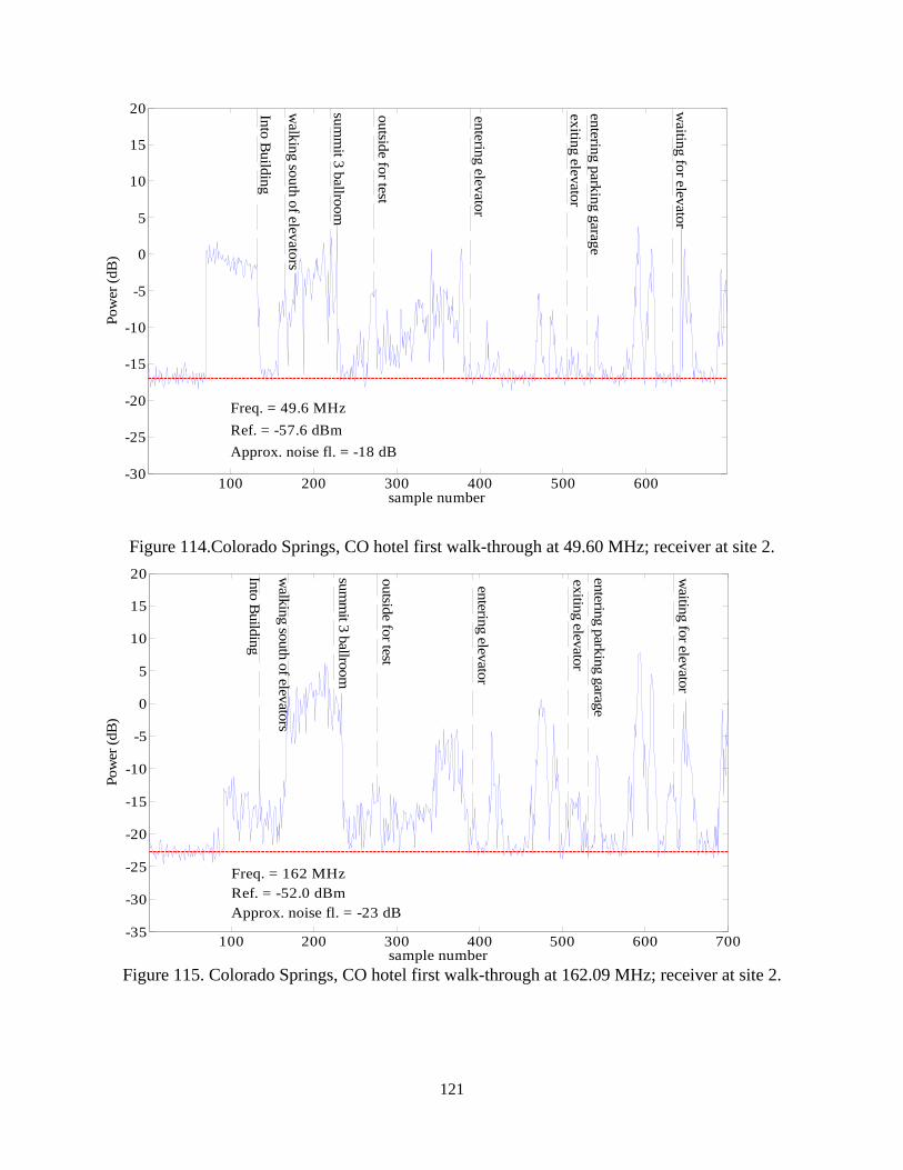
121

Figure 114.Colorado Springs, CO hotel first walk-through at 49.60 MHz; receiver at site 2.


100 200 300 400 500 600-30

-25

-20

-15

-10

-5

0

5

10

15

20

sample number

Pow

er (

dB)

Freq. = 49.6 MHz

Ref. = -57.6 dBm


Into Building


summ

it 3 ballroom

outside for test

entering elevator



100 200 300 400 500 600 700-35

-30

-25

-20

-15

-10

-5

0

5

10

15

20

sample number

Pow

er (

dB)


Into Building


summ

it 3 ballroom

outside for test

entering elevator

exiting elevator

entering parking garage


122



100 200 300 400 500 600 700-35

-30

-25

-20

-15

-10

-5

0

5

10

15

20

sample number

Pow

er (

dB)


Into Building


summ

it 3 ballroom

outside for test

entering elevator



100 200 300 400 500 600 700-40

-30

-20

-10

0

10

20

sample number

Pow

er (

dB)


Into Building


summ

it 3 ballroom

outside for test

entering elevator



123



100 200 300 400 500 600 700-35

-30

-25

-20

-15

-10

-5

0

5

10

15

20

sample number

Pow

er (

dB)


Into Building


summ

it 3 ballroom

outside for test

entering elevator

exiting elevator

entering parking garage


100 200 300 400 500 600 700-35

-30

-25

-20

-15

-10

-5

0

5

10

15

20

sample number

Pow

er (

dB)


Into Building


summ

it 3 ballroom

outside for test

entering elevator



124

Figure 120. Colorado Springs, CO hotel statistics, histograms, and empirical CDF for first walk-through data with the receiver at site 2; 49.60, 162.09, and 225.30 MHz.

Power (dB)

N

CD

F

-40 -35 -30 -25 -20 -15 -10 -5 0 5 100

20

40

60

80

100

freq. = 49 MHz

ref. = -57.6 dBm

median = -14.9 dB

mean = -12.3 dB

std. dev. = 5.3 dB

-40 -35 -30 -25 -20 -15 -10 -5 0 5 100

0.2

0.4

0.6

0.8

1

-40 -35 -30 -25 -20 -15 -10 -5 0 5 100

20

40

60

80

100

freq. = 162 MHz

ref. = -52.0 dBm

median = -17.5 dB

mean = -15.4 dB

std. dev. = 7.8 dB

-40 -35 -30 -25 -20 -15 -10 -5 0 5 100

0.2

0.4

0.6

0.8

1

-40 -35 -30 -25 -20 -15 -10 -5 0 5 100

20

40

60

80

100

freq. = 225 MHz

ref. = -50.9 dBm

median = -19.3 dB

mean = -16.8 dB

std. dev. = 7.6 dB

-40 -35 -30 -25 -20 -15 -10 -5 0 5 100

0.2

0.4

0.6

0.8

1

125

Power (dB)

N

CD

F

-40 -35 -30 -25 -20 -15 -10 -5 0 5 100

20

40

60

80

100

freq. = 449 MHz

ref. = -46.3 dBm

median = -22.7 dB

mean = -20.3 dB

std. dev. = 8.4 dB

-40 -35 -30 -25 -20 -15 -10 -5 0 5 100

0.2

0.4

0.6

0.8

1

-40 -35 -30 -25 -20 -15 -10 -5 0 5 100

20

40

60

80

100

freq. = 902 MHz

ref. = -49.1 dBm

median = -21.1 dB

mean = -18.1 dB

std. dev. = 7.9 dB

-40 -35 -30 -25 -20 -15 -10 -5 0 5 100

0.2

0.4

0.6

0.8

1

Figure 121. Colorado Springs, CO hotel statistics, histograms, and empirical CDF for first walk-through data with the receiver at site 2; 448.50 and 902.45 MHz.

126



100 200 300 400 500 600 700

-80

-70

-60

-50

-40

-30

-20

-10

0

10

20

sample number

Pow

er (

dB)


Into Building

level 9

passing elevators

landing level 11

passing elevator



entering elevators

entering elevators

power off

100 200 300 400 500 600 700

-80

-70

-60

-50

-40

-30

-20

-10

0

10

20

sample number

Pow

er (

dB)


Into Building

level 9

passing elevators

landing level 11

passing elevator



entering elevators

entering elevators

power off

127



100 200 300 400 500 600 700-80

-70

-60

-50

-40

-30

-20

-10

0

10

20

sample number

Pow

er (

dB)


Into Building

level 9

passing elevators

landing level 11

passing elevator



entering elevators

entering elevators

power off

100 200 300 400 500 600 700

-70

-60

-50

-40

-30

-20

-10

0

10

20

sample numbers

Pow

er (

dB)


Into Building

level 9

passing elevators

landing level 11

passing elevator



entering elevators

entering elevators

power off

128



100 200 300 400 500 600 700

-70

-60

-50

-40

-30

-20

-10

0

10

20

sample number

Pow

er (

dB)


Into Building

level 9

passing elevators

landing level 11

passing elevator



entering elevators

entering elevators

power off

100 200 300 400 500 600 700

-70

-60

-50

-40

-30

-20

-10

0

10

20

sample number

Pow

er (

dB)


Into Building

level 9

passing elevators

landing level 11

passing elevator



entering elevators

entering elevators

power off

129

Figure 128. Colorado Springs, CO hotel statistics, histograms, and empirical CDF for second walk-through data with the receiver at site 2; 49.60, 162.09, and 225.30 MHz.

Power (dB)

N

CD

F

-80 -70 -60 -50 -40 -30 -20 -10 0 100

25

50

75

100

125

freq. = 49 MHzref. = -31.5 dBm


-80 -70 -60 -50 -40 -30 -20 -10 0 100

0.2

0.4

0.6

0.8

1

-80 -70 -60 -50 -40 -30 -20 -10 0 100

10

20

30

40

50

freq. = 162 MHz

ref. = -32.8 dBm

median = -48.2 dB

mean = -46.6 dB

std. dev. = 11.8 dB

-80 -70 -60 -50 -40 -30 -20 -10 0 100

0.2

0.4

0.6

0.8

1

-80 -70 -60 -50 -40 -30 -20 -10 0 100

10

20

30

40

50

freq. = 225 MHz

ref. = -37.0 dBm

median = -46.8 dB

mean = -44.9 dB

std. dev. = 11.4 dB

-80 -70 -60 -50 -40 -30 -20 -10 0 100

0.2

0.4

0.6

0.8

1

130

Power (dB)

N

CD

F

-80 -70 -60 -50 -40 -30 -20 -10 0 100

10

20

30

40

50

freq. = 449 MHz

ref. = -42.9 dBm

median = -38.7 dB

mean = -36.3 dB

std. dev. = 12.1 dB

-80 -70 -60 -50 -40 -30 -20 -10 0 100

0.2

0.4

0.6

0.8

1

-80 -70 -60 -50 -40 -30 -20 -10 0 100

10

20

30

40

50

freq. = 902 MHz

ref. = -41.3 dBm

median = -44.9 dB

mean = -42.2 dB

std. dev. = 11.3 dB

-80 -70 -60 -50 -40 -30 -20 -10 0 100

0.2

0.4

0.6

0.8

1

Figure 129. Colorado Springs, CO hotel statistics, histograms, and empirical CDF for second walk-through data with the receiver at site 2; 448.50 and 902.45 MHz.

131

Figure 130. Boulder, CO grocery store walk-through at 49.60 MHz.


200 400 600 800 1000 1200 1400 1600

-80

-70

-60

-50

-40

-30

-20

-10

0

10

20

sample number

Pow

er (

dB)


Into Building

N.W

. corner S.W

. corner

S.E. corner

N.E

. corner

Into Building

Out of B

uilding

Walking backand forth alongthe aisles

200 400 600 800 1000 1200 1400

-80

-70

-60

-50

-40

-30

-20

-10

0

10

20

sample number

Pow

er (

dB)


Into Building

N.W

. corner

S.W. corner

S.E. corner

N.E

. corner

Into Building

Out of B

uildingWalking backand forth alongthe aisles

132



200 400 600 800 1000 1200 1400 1600

-80

-70

-60

-50

-40

-30

-20

-10

0

10

20

sample number

Pow

er (

dB)


Into Building

N.W

. corner

S.W. corner

S.E. corner

N.E

. corner

Into Building

Out of B


200 400 600 800 1000 1200 1400 1600

-80

-70

-60

-50

-40

-30

-20

-10

0

10

20

sample number

Pow

er (

dB)


Into Building

N.W

. corner

S.W. corner

S.E. corner

N.E

. corner

Into Building

Out of B

uilding


133



200 400 600 800 1000 1200 1400

-60

-50

-40

-30

-20

-10

0

10

20

sample number

Pow

er (

dB)

Freq. = 902 MHz

Ref. = -27.9 dBm


Into Building N

.W. corner

S.W. corner

S.E. corner

N.E

. corner

Into Building

Out of B

uilding


200 400 600 800 1000 1200 1400 1600-80

-70

-60

-50

-40

-30

-20

-10

0

10

20

sample number

Pow

er (

dB)


Into Building

N.W

. corner

S.W. corner

S.E. corner

N.E

. corner

Into Building

Out of B


134

Figure 136. Boulder, CO grocery store statistics, histograms, and empirical CDF for walk-through data; 49.60, 162.09, and 225.30 MHz.

Power (dB)

N

CD

F

-80 -70 -60 -50 -40 -30 -20 -10 0 10 200

20

40

60

80

100

freq. = 49 MHz

ref. = -35.4 dBm

median = -45.1 dB

mean = -43.1 dB

std. dev. = 12.0 dB

-80 -70 -60 -50 -40 -30 -20 -10 0 10 200

0.2

0.4

0.6

0.8

1

-80 -70 -60 -50 -40 -30 -20 -10 0 10 200

20

40

60

80

100

freq. = 162 MHz

ref. = -36.5 dBm

median = -38.6 dB

mean = -36.0 dB

std. dev. = 11.8 dB

-80 -70 -60 -50 -40 -30 -20 -10 0 10 200

0.2

0.4

0.6

0.8

1

-80 -70 -60 -50 -40 -30 -20 -10 0 10 200

20

40

60

80

100

freq. = 225 MHz

ref. = -32.6 dBm

median = -45.8 dB

mean = -43.0 dB

std. dev. = 14.5 dB

-80 -70 -60 -50 -40 -30 -20 -10 0 10 200

0.2

0.4

0.6

0.8

1

135

Figure 137. Boulder, CO grocery store statistics, histograms, and empirical CDF for walk-through data; 448.50, 902.75, and 1830.00 MHz.

Power (dB)

N

CD

F

-80 -70 -60 -50 -40 -30 -20 -10 0 10 200

20

40

60

80

100

freq. = 449 MHz

ref. = -34.6 dBm

median = -30.7 dB

mean = -29.2 dB

std. dev. = 11.7 dB

-80 -70 -60 -50 -40 -30 -20 -10 0 10 200

0.2

0.4

0.6

0.8

1

-80 -70 -60 -50 -40 -30 -20 -10 0 10 200

20

40

60

80

100

freq. = 902 MHz

ref. = -27.9 dBm

median = -35.3 dB

mean = -33.8 dB

std. dev. = 12.3 dB

-80 -70 -60 -50 -40 -30 -20 -10 0 10 200

0.2

0.4

0.6

0.8

1

-80 -70 -60 -50 -40 -30 -20 -10 0 10 200

20

40

60

80

100

freq. = 1830 MHz

ref. = -34.2 dBm

median = -40.8 dB

mean = -39.3 dB

std. dev. = 12.0 dB

-80 -70 -60 -50 -40 -30 -20 -10 0 10 200

0.2

0.4

0.6

0.8

1

136

Figure 138. Gaithersburg, MD office building walk-through at 49.60 MHz.


500 1000 1500 2000 2500-90

-80

-70

-60

-50

-40

-30

-20

-10

0

10

20

sample number

Pow

er (

dB)

Freq. = 49 MHz Ref. = -21.3 dBm Approx. noise fl. = -78 dB

Into Building

Basem

ent S.E.

Basem

ent N.W

.

L10 W

. stairs

L8 W

. stairs

L6 W

. stairs

L4 W

. stairs

L2 W

. stairs

L1 S.E

.

L1 S.W

500 1000 1500 2000 2500-80

-70

-60

-50

-40

-30

-20

-10

0

10

20

sample number

Pow

er (

dB)


Into Building

Basem

ent S.E.

Basem

ent N.W

.

L10 W

. stairs

L8 W

. stairs

L6 W

. stairs

L4 W

. stairs

L2 W

. stairs

L1 S.E

.

L1 S.W

137



500 1000 1500 2000-80

-70

-60

-50

-40

-30

-20

-10

0

10

20

sample number

Pow

er (

dB)


Into Building

Basem

ent S.E.

Basem

ent N.W

.

L10 W

. stairs

L8 W

. stairs

L6 W

. stairs

L4 W

. stairs

L2 W

. stairs

L1 S.E

.

L1 S.W

500 1000 1500 2000-80

-70

-60

-50

-40

-30

-20

-10

0

10

20

sample number

Pow

er (

dB)


Into Building

Basem

ent S.E.

Basem

ent N.W

.

L10 W

. stairs

L8 W

. stairs

L6 W

. stairs

L4 W

. stairs

L2 W

. stairs

L1 S.E

.

L1 S.W

138



500 1000 1500 2000-90

-80

-70

-60

-50

-40

-30

-20

-10

0

10

20

sample number

Pow

er (

dB)


Into Building

Basem

ent S.E.

Basem

ent N.W

.

L10 W

. stairs

L8 W

. stairs

L6 W

. stairs

L4 W

. stairs

L2 W

. stairs

L1 S.E

.

L1 S.W

500 1000 1500 2000-80

-70

-60

-50

-40

-30

-20

-10

0

10

20

sample number

Pow

er (

dB)


Into Building

Basem

ent S.E.

Basem

ent N.W

.

L10 W

. stairs

L8 W

. stairs

L6 W

. stairs

L4 W

. stairs

L2 W

. stairs

L1 S.E

.

L1 S.W

139

Figure 144. Gaithersburg, MD office building statistics, histograms, and empirical CDF for walk-through data; 49.60, 162.09, and 226.40 MHz.

Power (dB)

N

CD

F

-90 -80 -70 -60 -50 -40 -30 -20 -10 0 100

80

160

240

320

400

freq. = 49 MHz

ref. = -21.3 dBm

median = -68.6 dB

mean = -62.1 dB

std. dev. = 16.5 dB

-90 -80 -70 -60 -50 -40 -30 -20 -10 0 100

0.2

0.4

0.6

0.8

1

-80 -70 -60 -50 -40 -30 -20 -10 0 100

40

80

120

160

200

freq. = 162 MHz

ref. = -41.9 dBm

median = -42.8 dB

mean = -41.6 dB

std. dev. = 12.5 dB

-80 -70 -60 -50 -40 -30 -20 -10 0 100

0.2

0.4

0.6

0.8

1

-80 -70 -60 -50 -40 -30 -20 -10 0 100

40

80

120

160

200

freq. = 226 MHz

ref. = -30.6 dBm

median = -44.7 dB

mean = -44.1 dB

std. dev. = 14.7 dB

-80 -70 -60 -50 -40 -30 -20 -10 0 100

0.2

0.4

0.6

0.8

1

140

Figure 145. Gaithersburg, MD office building statistics, histograms, and empirical CDF for walk-through data; 448.30, 902.45, and 1830.00 MHz.

Power (dB)

N

CD

F

-80 -70 -60 -50 -40 -30 -20 -10 0 100

40

80

120

160

200

freq. = 448 MHz

ref. = -30.1 dBm

median = -46.7 dB

mean = -46.9 dB

std. dev. = 14.1 dB

-80 -70 -60 -50 -40 -30 -20 -10 0 100

0.2

0.4

0.6

0.8

1

-80 -70 -60 -50 -40 -30 -20 -10 0 100

40

80

120

160

200

freq. = 902 MHz

ref. = -21.8 dBm

median = -59.7 dB

mean = -57.7 dB

std. dev. = 14.6 dB

-80 -70 -60 -50 -40 -30 -20 -10 0 100

0.2

0.4

0.6

0.8

1

-80 -70 -60 -50 -40 -30 -20 -10 0 100

80

160

240

320

400

freq. = 1830 MHz

ref. = -30.6 dBm

median = -59.9 dB

mean = -55.6 dB

std. dev. = 12.2 dB

-80 -70 -60 -50 -40 -30 -20 -10 0 100

0.2

0.4

0.6

0.8

1

141

Figure 146. Bethesda, MD shopping mall walk-through at 49.60 MHz; receiver at site 1.

500

1000

1500

2000

2500

3000

3500

4000

4500

-70

-60

-50

-40

-30

-20

-1001020

sam

ple

num

ber

Power (dB)

Freq

. = 4

9 M

Hz

Ref

. = -

47.3

dB

m

App

rox.

noi

se f

l. =

-52

dB

LOS outside

Inside Mall

1st Hall2nd HallSears

LOS Sears

Inside, Sears2nd HallHechts

LOS, food courtHechts1st Hall

Nordstrom, upper

Nordstrom, lower

1st Hall, Santa1st Hall, BebeSearsLOS, Sears

Inside Mall, Sears1st Hall, Bebe

End of Hall

Side Hallway, lower

Side Hallway, lower

Inside Mall, Hechts

LOS, oustide Hechts

142


500

1000

1500

2000

2500

3000

3500

-70

-60

-50

-40

-30

-20

-1001020

sam

ple

num

ber

Power (dB)

Freq

. = 1

62 M

Hz

Ref

. = -

48.7

dB

m

App

rox.

noi

se f

l. =

-50

dB

LOS outside

Inside Mall


LOS Sears

Inside, Sears2nd Hall

Hechts

LOS, food court

Hechts

1st Hall

Nordstrom, upper

Nordstrom, lower

1st Hall, Santa1st Hall, BebeSears

LOS, Sears


End of Hall

Side Hallway, lower

Side Hallway, lower

Inside Mall, Hechts

LOS, oustide Hechts

143


500

1000

1500

2000

2500

3000

-70

-60

-50

-40

-30

-20

-1001020

sam

ple

num

ber

Power (dB)

Freq

. = 2

26 M

Hz

Ref

. = -

41.7

dB

m

App

rox.

noi

se f

l. =

-58

dB

LOS outside

Inside Mall


LOS Sears


Hechts

LOS, food court

Hechts

1st Hall

Nordstrom, upper

Nordstrom, lower1st Hall, Santa

1st Hall, BebeSears

LOS, Sears


End of Hall

Side Hallway, lower

Side Hallway, lowerInside Mall, Hechts

LOS, oustide Hechts

144


500

1000

1500

2000

2500

3000

3500

-70

-60

-50

-40

-30

-20

-1001020

sam

ple

num

ber

Power (dB)

Freq

. = 4

48 M

Hz

Ref

. = -

41.8

dB

m

App

rox.

noi

se f

l. =

-56

dB

LOS outside

Inside Mall


LOS Sears

Inside, Sears

2nd Hall

Hechts

LOS, food court

Hechts1st Hall

Nordstrom, upper


1st Hall, BebeSears

LOS, Sears


End of Hall

Side Hallway, lowerSide Hallway, lowerInside Mall, Hechts

LOS, oustide Hechts

145


500

1000

1500

2000

2500

3000

3500

4000

-60

-50

-40

-30

-20

-1001020

sam

ple

num

ber

Power (dB)

Freq

. = 9

02 M

Hz

Ref

. = -

49.0

dB

m

App

rox.

noi

se f

l. =

-49

dB

m

LOS outside

Inside Mall


LOS Sears


Hechts

LOS, food court

Hechts1st Hall

Nordstrom, upper

Nordstrom, lower

1st Hall, Santa

1st Hall, BebeSears

LOS, Sears


End of Hall

Side Hallway, lower

Side Hallway, lower

Inside Mall, Hechts

LOS, oustide Hechts

146

Figure 151. Bethesda, MD shopping mall walk-through at 1830.00 MHz;

receiver at site 1.

500

1000

1500

2000

2500

3000

3500

-50

-40

-30

-20

-1001020

sam

ple

num

ber

Power (dB)

Freq

. = 1

830

MH

z

Ref

. = -

62.2

dB

m

App

rox.

noi

se f

l. =

-35

dB

LOS outside

Inside Mall1st Hall

2nd HallSears

LOS Sears


Hechts

LOS, food court

Hechts1st Hall

Nordstrom, upper

Nordstrom, lower 1st Hall, Santa

1st Hall, BebeSears

LOS, Sears


End of Hall

Side Hallway, lower

Side Hallway, lower

Inside Mall, Hechts

LOS, oustide Hechts

147

Figure 152. Bethesda, MD shopping mall statistics, histograms, and empirical CDF for walk-through data with the receiver at site 1; 49.60, 162.09, and 226.40 MHz.

Power (dB)

N

CD

F

-80 -70 -60 -50 -40 -30 -20 -10 0 100

200

400

600

800

1000

freq. = 49 MHz

ref. = -47.3 dBm

median = -49.4 dB

mean = -47.2 dB

std. dev. = 5.9 dB

-80 -70 -60 -50 -40 -30 -20 -10 0 100

0.2

0.4

0.6

0.8

1

-80 -70 -60 -50 -40 -30 -20 -10 0 100

200

400

600

800

1000

freq. = 162 MHz

ref. = -48.7 dBm

median = -48.6 dB

mean = -46.5 dB

std. dev. = 5.8 dB

-80 -70 -60 -50 -40 -30 -20 -10 0 100

0.2

0.4

0.6

0.8

1

-80 -70 -60 -50 -40 -30 -20 -10 0 100

200

400

600

800

1000

freq. = 226 MHz

ref. = -41.7 dBm

median = -51.6 dB

mean = -49.9 dB

std. dev. = 7.1 dB

-80 -70 -60 -50 -40 -30 -20 -10 0 100

0.2

0.4

0.6

0.8

1

148


N

CD

F

-80 -70 -60 -50 -40 -30 -20 -10 0 100

200

400

600

800

1000

freq. = 448 MHz

ref. = -41.8 dBm

median = -54.7 dB

mean = -52.8 dB

std. dev. = 5.6 dB

-80 -70 -60 -50 -40 -30 -20 -10 0 100

0.2

0.4

0.6

0.8

1

-80 -70 -60 -50 -40 -30 -20 -10 0 100

200

400

600

800

1000

freq. = 902 MHz

ref. = -49.0 dBm

median = -47.2 dB

mean = -44.6 dB

std. dev. = 6.3 dB

-80 -70 -60 -50 -40 -30 -20 -10 0 100

0.2

0.4

0.6

0.8

1

-80 -70 -60 -50 -40 -30 -20 -10 0 100

200

400

600

800

1000

freq. = 1830 MHz

ref. = -62.2 dBm

median = -34.1 dB

mean = -33.3 dB

std. dev. = 3.9 dB

-80 -70 -60 -50 -40 -30 -20 -10 0 100

0.2

0.4

0.6

0.8

1

149


500

1000

1500

2000

2500

3000

3500

4000

-70

-60

-50

-40

-30

-20

-1001020

sam

ple

num

ber

Power (dB)

Freq

. = 4

9 M

Hz

Ref

. = -

48.9

dB

m

App

rox.

noi

se f

l. =

-51

dB

LOS outside

Inside Mall


LOS Sears


Hechts

LOS, food court

Hechts1st Hall

Nordstrom, upper

Nordstrom, lower


LOS, Sears


End of Hall

Side Hallway, lower

Side Hallway, lower

Inside Mall, Hechts

LOS, oustide Hechts

150


500

1000

1500

2000

2500

3000

3500

-60

-50

-40

-30

-20

-1001020

sam

ple

num

ber

Power (dB)

Freq

. = 1

62 M

Hz

Ref

. = -

55.2

dB

m

App

rox.

noi

se f

l. =

-44

dB

LOS outside

Inside Mall


LOS Sears


Hechts

LOS, food court

Hechts

1st HallNordstrom, upper

Nordstrom, lower


LOS, Sears


End of Hall

Side Hallway, lower


LOS, oustide Hechts

151


500

1000

1500

2000

2500

3000

-70

-60

-50

-40

-30

-20

-1001020

sam

ple

num

ber

Power (dB)

Freq

. = 2

26 M

Hz

Ref

. = -

45.6

dB

m

App

rox.

noi

se f

l. =

-53

dB

LOS outside

Inside Mall


LOS Sears


Hechts

LOS, food court

Hechts

1st Hall

Nordstrom, upper


1st Hall, BebeSears

LOS, Sears


End of Hall

Side Hallway, lower


LOS, oustide Hechts

152


500

1000

1500

2000

2500

3000

-60

-50

-40

-30

-20

-1001020

sam

ple

num

ber

Power (dB)

Freq

. = 4

48 M

Hz

Ref

. = -

52.4

dB

m

App

rox.

noi

se f

l. =

-47

dB

LOS outside

Inside Mall


LOS Sears


Hechts

LOS, food court

Hechts1st Hall

Nordstrom, upper


1st Hall, BebeSearsLOS, Sears


End of Hall

Side Hallway, lower


LOS, oustide Hechts

153


500

1000

1500

2000

2500

3000

3500

-70

-60

-50

-40

-30

-20

-1001020

sam

ple

num

ber

Power (dB)

Freq

. = 9

02 M

Hz

Ref

. = -

41.1

dB

m

App

rox.

noi

se f

l. =

-58

dB

LOS outside

Inside Mall


LOS Sears

Inside, Sears

2nd Hall

Hechts

LOS, food court

Hechts

1st Hall

Nordstrom, upper

Nordstrom, lower

1st Hall, Santa

1st Hall, BebeSearsLOS, Sears


End of Hall

Side Hallway, lower

Side Hallway, lower

Inside Mall, Hechts

LOS, oustide Hechts

154

Figure 159. Bethesda, MD shopping mall walk-through at 1830.00 MHz;

receiver at site 2.

500

1000

1500

2000

2500

3000

-60

-50

-40

-30

-20

-1001020

sam

ple

num

ber

Power (dB)

Freq

. = 1

830

MH

z

Ref

. = -

55.0

dB

m

App

rox.

noi

se f

l. =

-42

dB

LOS outside

Inside Mall1st Hall

2nd HallSears

LOS Sears


Hechts

LOS, food court

Hechts1st Hall

Nordstrom, upper


1st Hall, BebeSears

LOS, Sears


End of Hall

Side Hallway, lower


LOS, oustide Hechts

155


Power (dB)

N

CD

F

-80 -70 -60 -50 -40 -30 -20 -10 0 100

100

200

300

400

500

freq. = 49 MHz

ref. = -48.9 dBm

median = -44.4 dB

mean = -42.2 dB

std. dev. = 9.7 dB

-80 -70 -60 -50 -40 -30 -20 -10 0 100

0.2

0.4

0.6

0.8

1

-80 -70 -60 -50 -40 -30 -20 -10 0 100

100

200

300

400

500

freq. = 162 MHz

ref. = -55.2 dBm

median = -38.0 dB

mean = -35.8 dB

std. dev. = 8.1 dB

-80 -70 -60 -50 -40 -30 -20 -10 0 100

0.2

0.4

0.6

0.8

1

-80 -70 -60 -50 -40 -30 -20 -10 0 100

100

200

300

400

500

freq. = 226 MHz

ref. = -45.6 dBm

median = -41.7 dB

mean = -39.8 dB

std. dev. = 11.1 dB

-80 -70 -60 -50 -40 -30 -20 -10 0 100

0.2

0.4

0.6

0.8

1

156


Power (dB)

N

CD

F

-80 -70 -60 -50 -40 -30 -20 -10 0 100

100

200

300

400

500

freq. = 448 MHz

ref. = -52.4 dBm

median = -39.9 dB

mean = -35.7 dB

std. dev. = 12.2 dB

-80 -70 -60 -50 -40 -30 -20 -10 0 100

0.2

0.4

0.6

0.8

1

-80 -70 -60 -50 -40 -30 -20 -10 0 100

100

200

300

400

500

freq. = 902 MHz

ref. = -41.1 dBm

median = -54.5 dB

mean = -50.4 dB

std. dev. = 11.2 dB

-80 -70 -60 -50 -40 -30 -20 -10 0 100

0.2

0.4

0.6

0.8

1

-80 -70 -60 -50 -40 -30 -20 -10 0 100

200

400

600

800

1000

freq. = 1830 MHz

ref. = -55.0 dBm

median = -41.0 dB

mean = -37.7 dB

std. dev. = 8.5 dB

-80 -70 -60 -50 -40 -30 -20 -10 0 100

0.2

0.4

0.6

0.8

1

157

Figure 162. Silver Spring, MD office building walk-through at 49.60 MHz.

1000

2000

3000

4000

5000

6000

-100-8

0

-60

-40

-20020

sam

ple

num

ber

Power (dB)

Freq

. = 4

9 M

Hz

Ref

. = -

21.6

dB

m

App

rox.

noi

se f

l. =

-78

dB

lobby

9C

9A7A7C

7H

7A5A5C

5H

5A3A3C

3H

3A1A

1C

1F

lobby elevatorba

sem

ent

158


500

1000

1500

2000

2500

3000

3500

4000

-90

-80

-70

-60

-50

-40

-30

-20

-1001020

sam

ple

num

ber

Power (dB)

Freq

. = 1

62 M

Hz

Ref

. = -

30.9

dB

m

App

rox.

noi

se f

l. =

-67

dB

lobby

9C9A7A7C

7H

7A5A5C

5H5A3A3C

3H

3A1A1C

1F

lobby elevator

base

men

t

159


500

1000

1500

2000

2500

3000

3500

-100-8

0

-60

-40

-20020

sam

ple

num

ber

Power (dB)

Freq

. = 2

26 M

Hz

Ref

. = -

21.7

dB

m

App

rox.

noi

se f

l. =

-78

dB

lobby

9C

9A7A7C

7H

7A5A

5C

5H

5A3A3C

3H

3A1A1C

1F

lobby elevator

base

men

t

160


500

1000

1500

2000

2500

3000

-90

-80

-70

-60

-50

-40

-30

-20

-1001020

sam

ple

num

ber

Power (dB)

Freq

. = 4

48 M

Hz

Ref

. = -

29.6

dB

m

App

rox.

noi

se f

l. =

-70

dB

lobby

9C

9A7A7C

7H

7A5A5C

5H

5A3A3C

3H

3A1A1C

1F

lobby elevator

base

men

t

161


500

1000

1500

2000

2500

3000

3500

-100-8

0

-60

-40

-20020

sam

ple

num

ber

Power (dB)

Freq

. = 9

02 M

Hz

Ref

. = -

16.0

dB

m

App

rox.

noi

se f

l. =

-83

dB

lobby

9C

9A7A7C

7H7A5A5C

5H

5A3A3C

3H3A1A1C1F

lobby elevatorba

sem

ent

162


500

1000

1500

2000

2500

3000

3500

-90

-80

-70

-60

-50

-40

-30

-20

-1001020

sam

ple

num

ber

Power (dB)

Freq

. = 1

830

MH

z

Ref

. = -

25.9

dB

m

App

rox.

noi

se f

l. =

-71

dB

lobby

9C

9A7A7C

7H7A5A5C

5H5A3A3C

3H

3A1A1C

1F

lobby elevator

base

men

t

163

Figure 168. Silver Spring, MD office building statistics, histograms, and empirical CDF for walk-through data; 49.60, 162.09, and 226.40 MHz.

Power (dB)

N

CD

F

-90 -80 -70 -60 -50 -40 -30 -20 -10 0 100

100

200

300

400

500

freq. = 49 MHz

ref. = -21.6 dBm

median = -64.2 dB

mean = -63.7 dB

std. dev. = 11.4 dB

-90 -80 -70 -60 -50 -40 -30 -20 -10 0 100

0.2

0.4

0.6

0.8

1

-90 -80 -70 -60 -50 -40 -30 -20 -10 0 100

100

200

300

400

500

freq. = 162 MHz

ref. = -30.9 dBm

median = -57.9 dB

mean = -55.7 dB

std. dev. = 10.3 dB

-90 -80 -70 -60 -50 -40 -30 -20 -10 0 100

0.2

0.4

0.6

0.8

1

-90 -80 -70 -60 -50 -40 -30 -20 -10 0 100

100

200

300

400

500

freq. = 226 MHz

ref. = -21.7 dBm

median = -61.3 dB

mean = -60.3 dB

std. dev. = 11.1 dB

-90 -80 -70 -60 -50 -40 -30 -20 -10 0 100

0.2

0.4

0.6

0.8

1

164

Figure 169. Silver Spring, MD office building statistics, histograms, and empirical CDF for walk-through data; 448.30, 902.45, and 1830.00 MHz.

Power (dB)

N

CD

F

-90 -80 -70 -60 -50 -40 -30 -20 -10 0 100

100

200

300

400

500

freq. = 448 MHz

ref. = -29.6 dBm

median = -52.6 dB

mean = -52.4 dB

std. dev. = 11.2 dB

-90 -80 -70 -60 -50 -40 -30 -20 -10 0 100

0.2

0.4

0.6

0.8

1

-90 -80 -70 -60 -50 -40 -30 -20 -10 0 100

100

200

300

400

500

freq. = 902 MHz

ref. = -16.0 dBm

median = -72.1 dB

mean = -70.4 dB

std. dev. = 10.5 dB

-90 -80 -70 -60 -50 -40 -30 -20 -10 0 100

0.2

0.4

0.6

0.8

1

-90 -80 -70 -60 -50 -40 -30 -20 -10 0 100

200

400

600

800

1000

freq. = 1830 MHz

ref. = -25.9 dBm

median = -69.5 dB

mean = -67.2 dB

std. dev. = 5.7 dB

-90 -80 -70 -60 -50 -40 -30 -20 -10 0 100

0.2

0.4

0.6

0.8

1

165

Figure 170. Washington, DC convention center walk-through at 49.60 MHz; receiver at site 1.


500 1000 1500 2000 2500 3000 3500 4000 4500 5000

-90

-80

-70

-60

-50

-40

-30

-20

-10

0

10

20

sample number

Pow

er (

dB)


Into Building

N.W

.-C-upper

S.E.-B

-upper

mid. level

N.W

.-C-low

er

S.E.-B

-lower

exit building

entering building

tower, 1st level

bottom stairs

500 1000 1500 2000 2500 3000 3500 4000 4500 5000

-90

-80

-70

-60

-50

-40

-30

-20

-10

0

10

20

sample number

Pow

er (

dB)


Into Building

N.W

.-C-upper

S.E.-B

-upper

mid. level

N.W

.-C-low

er

S.E.-B

-lower

exit building

entering buildingtow

er, 1st level

bottom stairs

166



500 1000 1500 2000 2500 3000 3500 4000 4500 5000

-100

-80

-60

-40

-20

0

20

sample number

Pow

er (

dB)


Into Building

N.W

.-C-upper

S.E.-B

-upper

mid. level

N.W

.-C-low

er

S.E.-B

-lower

exit building


er, 1st level

bottom stairs

500 1000 1500 2000 2500 3000 3500 4000 4500 5000-100

-80

-60

-40

-20

0

20

sample number

Pow

er (

dB)


Into Building

N.W

.-C-upper

S.E.-B

-upper

mid. level

N.W

.-C-low

er

S.E.-B

-lower

exit building


er, 1st level

bottom stairs

167



500 1000 1500 2000 2500 3000 3500 4000 4500-100

-80

-60

-40

-20

0

20

sample number

Pow

er (

dB)


Into Building

N.W

.-C-upper

S.E.-B

-upper

mid. level

N.W

.-C-low

er

S.E.-B

-lower

exit building


er, 1st level

bottom stairs

500 1000 1500 2000 2500 3000 3500 4000-90

-80

-70

-60

-50

-40

-30

-20

-10

0

10

20

sample number

Pow

er (

dB)


Into Building

N.W

.-C-upper

S.E.-B

-upper

mid. level

N.W

.-C-low

er

S.E.-B

-lower

exit building

entering building

tower, 1st level

bottom stairs

168

Figure 176. Washington, DC convention center statistics, histograms, and empirical CDF for walk-through data with the receiver at site 1; 49.60, 162.09, and 226.40 MHz.

Power (dB)

N

CD

F

-90 -80 -70 -60 -50 -40 -30 -20 -10 0 100

100

200

300

400

500

freq. = 49 MHz

ref. = -19.1 dBm

median = -63.9 dB

mean = -62.3 dB

std. dev. = 12.5 dB

-90 -80 -70 -60 -50 -40 -30 -20 -10 0 100

0.2

0.4

0.6

0.8

1

-90 -80 -70 -60 -50 -40 -30 -20 -10 0 100

100

200

300

400

500

freq. = 162 MHz

ref. = -26.3 dBm

median = -61.9 dB

mean = -59.9 dB

std. dev. = 12.1 dB

-90 -80 -70 -60 -50 -40 -30 -20 -10 0 100

0.2

0.4

0.6

0.8

1

-100 -90 -80 -70 -60 -50 -40 -30 -20 -10 0 100

100

200

300

400

500

freq. = 226 MHz

ref. = -9.1 dBm

median = -65.3 dB

mean = -64.1 dB

std. dev. = 13.3 dB

-100 -90 -80 -70 -60 -50 -40 -30 -20 -10 0 100

0.2

0.4

0.6

0.8

1

169


Power (dB)

N

CD

F

-90 -80 -70 -60 -50 -40 -30 -20 -10 0 100

100

200

300

400

500

freq. = 448 MHz

ref. = -18.6 dBm

median = -56.2 dB

mean = -54.7 dB

std. dev. = 14.0 dB

-90 -80 -70 -60 -50 -40 -30 -20 -10 0 100

0.2

0.4

0.6

0.8

1

-90 -80 -70 -60 -50 -40 -30 -20 -10 0 100

100

200

300

400

500

freq. = 902 MHz

ref. = -16.5 dBm

median = -63.8 dB

mean = -61.8 dB

std. dev. = 14.5 dB

-90 -80 -70 -60 -50 -40 -30 -20 -10 0 100

0.2

0.4

0.6

0.8

1

-90 -80 -70 -60 -50 -40 -30 -20 -10 0 100

100

200

300

400

500

freq. = 1830 MHz

ref. = -27.5 dBm

median = -60.8 dB

mean = -57.9 dB

std. dev. = 11.4 dB

-90 -80 -70 -60 -50 -40 -30 -20 -10 0 100

0.2

0.4

0.6

0.8

1

170



500 1000 1500 2000 2500 3000 3500 4000 4500 5000 5500-90

-80

-70

-60

-50

-40

-30

-20

-10

0

10

20

sample number

Pow

er (

dB)


Into Building

N.W

.-C-upper

S.E.-B

-upper

mid. level

N.W

.-C-low

er

S.E.-B

-lower

exit building


er, 1st level

bottom stairs

500 1000 1500 2000 2500 3000 3500 4000 4500 5000 5500-100

-80

-60

-40

-20

0

20

sample number

Pow

er (

dB)


Into Building

N.W

.-C-upper

S.E.-B

-upper

mid. level

N.W

.-C-low

er

S.E.-B

-lower

exit building


er, 1st level

bottom stairs

171



500 1000 1500 2000 2500 3000 3500 4000 4500 5000-100

-80

-60

-40

-20

0

20

sample number

Pow

er (

dB)


Into Building

N.W

.-C-upper

S.E.-B

-upper

mid. level

N.W

.-C-low

er

S.E.-B

-lower

exit building


er, 1st level

bottom stairs

500 1000 1500 2000 2500 3000 3500 4000 4500 5000-100

-80

-60

-40

-20

0

20

sample number

Pow

er (

dB)


Into Building

N.W

.-C-upper

S.E.-B

-upper

mid. level

N.W

.-C-low

er

S.E.-B

-lower

exit building


er, 1st level

bottom stairs

172



500 1000 1500 2000 2500 3000 3500 4000 4500 5000

-90

-80

-70

-60

-50

-40

-30

-20

-10

0

10

20

sample number

Pow

er (

dB)


Into Building

N.W

.-C-upper

S.E.-B

-upper

mid. level

N.W

.-C-low

er

S.E.-B

-lower

exit building


er, 1st level

bottom stairs

500 1000 1500 2000 2500 3000 3500 4000 4500 5000-90

-80

-70

-60

-50

-40

-30

-20

-10

0

10

20

sample number

Pow

er (

dB)


Into Building

N.W

.-C-upper

S.E.-B

-upper

mid. level

N.W

.-C-low

er

S.E.-B

-lower

exit building

entering building

tower, 1st level

bottom stairs

173


Power (dB)

N

CD

F

-90 -80 -70 -60 -50 -40 -30 -20 -10 0 100

100

200

300

400

500

freq. = 49 MHz

ref. = -26.3 dBm

median = -50.6 dB

mean = -49.8 dB

std. dev. = 14.4 dB

-90 -80 -70 -60 -50 -40 -30 -20 -10 0 100

0.2

0.4

0.6

0.8

1

-90 -80 -70 -60 -50 -40 -30 -20 -10 0 100

100

200

300

400

500

freq. = 162 MHz

ref. = -21.3 dBm

median = -65.0 dB

mean = -61.1 dB

std. dev. = 15.3 dB

-90 -80 -70 -60 -50 -40 -30 -20 -10 0 100

0.2

0.4

0.6

0.8

1

-90 -80 -70 -60 -50 -40 -30 -20 -10 0 100

100

200

300

400

500

freq. = 226 MHz

ref. = -15.8 dBm

median = -58.8 dB

mean = -56.8 dB

std. dev. = 14.6 dB

-90 -80 -70 -60 -50 -40 -30 -20 -10 0 100

0.2

0.4

0.6

0.8

1

174


Power (dB)

N

CD

F

-90 -80 -70 -60 -50 -40 -30 -20 -10 0 100

100

200

300

400

500

freq. = 448 MHz

ref. = -18.2 dBm

median = -58.1 dB

mean = -56.9 dB

std. dev. = 13.4 dB

-90 -80 -70 -60 -50 -40 -30 -20 -10 0 100

0.2

0.4

0.6

0.8

1

-90 -80 -70 -60 -50 -40 -30 -20 -10 0 100

100

200

300

400

500

freq. = 902 MHz

ref. = -23.5 dBm

median = -55.4 dB

mean = -54.0 dB

std. dev. = 13.7 dB

-90 -80 -70 -60 -50 -40 -30 -20 -10 0 100

0.2

0.4

0.6

0.8

1

-90 -80 -70 -60 -50 -40 -30 -20 -10 0 100

100

200

300

400

500

freq. = 1830 MHz

ref. = -25.5 dBm

median = -60.1 dB

mean = -58.0 dB

std. dev. = 11.8 dB

-90 -80 -70 -60 -50 -40 -30 -20 -10 0 100

0.2

0.4

0.6

0.8

1

175



500 1000 1500 2000 2500 3000 3500 4000 4500 5000

-100

-80

-60

-40

-20

0

20

sample number

Pow

er (

dB)


Into Building

N.W

.-C-upper

S.E.-B

-upper

mid. level

N.W

.-C-low

er

S.E.-B

-lower

exit building


er, 1st level

bottom stairs

1000 2000 3000 4000 5000 6000

-100

-80

-60

-40

-20

0

20

sample number

Pow

er (

dB)


Into Building

N.W

.-C-upper

S.E.-B

-upper

mid. level

N.W

.-C-low

er

S.E.-B

-lower

exit building

entering building

tower, 1st level

bottom stairs

176



500 1000 1500 2000 2500 3000 3500 4000 4500 5000

-100

-80

-60

-40

-20

0

20

sample number

Pow

er (

dB)


Into Building

N.W

.-C-upper

S.E.-B

-upper

mid. level

N.W

.-C-low

er

S.E.-B

-lower

exit building


er, 1st level

bottom stairs

500 1000 1500 2000 2500 3000 3500 4000 4500 5000 5500

-100

-80

-60

-40

-20

0

20

sample number

Pow

er (

dB)


Into Building

N.W

.-C-upper

S.E.-B

-upper

mid. level

N.W

.-C-low

er

S.E.-B

-lower

exit building


er, 1st level

bottom stairs

177



500 1000 1500 2000 2500 3000 3500 4000 4500

-100

-80

-60

-40

-20

0

20

sample number

Pow

er (

dB)


Into Building

N.W

.-C-upper

S.E.-B

-upper

mid. level

N.W

.-C-low

er

S.E.-B

-lower

exit building


er, 1st level

bottom stairs

500 1000 1500 2000 2500 3000 3500 4000 4500-90

-80

-70

-60

-50

-40

-30

-20

-10

0

10

20

sample number

Pow

er (

dB)


Into Building

N.W

.-C-upper

S.E.-B

-upper

mid. level

N.W

.-C-low

er

S.E.-B

-lower

exit building

entering building

tower, 1st level

bottom stairs

178


Power (dB)

N

CD

F

-90 -80 -70 -60 -50 -40 -30 -20 -10 0 100

40

80

120

160

200

freq. = 49 MHz

ref. = -13.3 dBm

median = -67.4 dB

mean = -65.3 dB

std. dev. = 15.5 dB

-90 -80 -70 -60 -50 -40 -30 -20 -10 0 100

0.2

0.4

0.6

0.8

1

-90 -80 -70 -60 -50 -40 -30 -20 -10 0 100

80

160

240

320

400

freq. = 162 MHz

ref. = -16.9 dBm

median = -68.9 dB

mean = -66.0 dB

std. dev. = 14.4 dB

-90 -80 -70 -60 -50 -40 -30 -20 -10 0 100

0.2

0.4

0.6

0.8

1

-100 -90 -80 -70 -60 -50 -40 -30 -20 -10 0 100

40

80

120

160

200

freq. = 226 MHz

ref. = -7.5 dBm

median = -64.2 dB

mean = -62.3 dB

std. dev. = 15.4 dB

-100 -90 -80 -70 -60 -50 -40 -30 -20 -10 0 100

0.2

0.4

0.6

0.8

1

179


Power (dB)

N

CD

F

-90 -80 -70 -60 -50 -40 -30 -20 -10 0 100

40

80

120

160

200

freq. = 448 MHz

ref. = -14.3 dBm

median = -58.9 dB

mean = -57.3 dB

std. dev. = 15.1 dB

-90 -80 -70 -60 -50 -40 -30 -20 -10 0 100

0.2

0.4

0.6

0.8

1

-100 -90 -80 -70 -60 -50 -40 -30 -20 -10 0 100

40

80

120

160

200

freq. = 902 MHz

ref. = -9.4 dBm

median = -68.5 dB

mean = -66.4 dB

std. dev. = 14.1 dB

-100 -90 -80 -70 -60 -50 -40 -30 -20 -10 0 100

0.2

0.4

0.6

0.8

1

-90 -80 -70 -60 -50 -40 -30 -20 -10 0 100

80

160

240

320

400

freq. = 1830 MHz

ref. = -24.6 dBm

median = -60.7 dB

mean = -58.2 dB

std. dev. = 12.1 dB

-90 -80 -70 -60 -50 -40 -30 -20 -10 0 100

0.2

0.4

0.6

0.8

1

180

Figure 194. Boulder, CO apartment walk-through at 162.075 MHz; receiver at site 1.

500 1000 1500 2000 2500 3000-80

-70

-60

-50

-40

-30

-20

-10

0

10

20

sample number

Pow

er (

dB)


L1

L2 A

pmt

L2 N

L3 S

L4 N

L5 S

L6 N

L7 A

pmt

L7 S

L8 N

L9 S

L10 N

L11 S

181



500 1000 1500 2000 2500 3000-80

-70

-60

-50

-40

-30

-20

-10

0

10

20

sample number

Pow

er (

dB)


L1

L2 A

pmt

L2 N

L3 S

L4 N

L5 S

L6 N

L7 A

pmt

L7 S

L8 N

L9 S

L10 N

L11 S

500 1000 1500 2000 2500 3000 3500-80

-70

-60

-50

-40

-30

-20

-10

0

10

20

sample number

Pow

er (

dB)


L1

L2 A

pmt

L2 N

L3 S

L4 N

L5 S

L6 N

L7 A

pmt

L7 S

L8 N

L9 S

L10 N

L11 S

182



500 1000 1500 2000 2500 3000-80

-70

-60

-50

-40

-30

-20

-10

0

10

20

sample number

Pow

er (

dB)


L1

L2 A

pmt

L2 N

L3 S

L4 N

L5 S

L6 N

L7 A

pmt

L7 S

L8 N

L9 S

L10 N

L11 S

500 1000 1500 2000 2500 3000 3500-80

-70

-60

-50

-40

-30

-20

-10

0

10

20

sample number

Pow

er (

dB)


L1

L2 A

pmt

L2 N

L3 S

L4 N

L5 S

L6 N

L7 A

pmt

L7 S

L8 N

L9 S

L10 N

L11 S

183

Figure 199. Boulder, CO apartment walk-through at 2445 MHz; receiver at site 1

Figure 200. Boulder, CO apartment walk-through at 4900 MHz; receiver at site 1

2000 4000 6000 8000 10000 12000-80

-70

-60

-50

-40

-30

-20

-10

0

10

20

sample number

Pow

er (

dB)


L1

L2 A

pmt

L2 N

L3 S

L4 N

L5 S

L6 N

L7 A

pmt

L7 S

L8 N

L9 S

L10 N

L11 S

2000 4000 6000 8000 10000 12000 14000-80

-70

-60

-50

-40

-30

-20

-10

0

10

20

sample number

Pow

er (

dB)


L1

L2 A

pmt

L2 N

L3 S

L4 N

L5 S

L6 N

L7 A

pmt

L7 S

L8 N

L9 S

L10 N

L11 S

184

Figure 201. Boulder, CO apartment walk-through statistics, histograms, and empirical CDF for walk-through data with the receiver at site 1; 162.075, 230.0 and 439.25 MHz.

Power (dB)

N

CD

F

-80 -70 -60 -50 -40 -30 -20 -10 0 10 200

40

80

120

160

200

freq. = 162 MHz

ref. = -17.0 dBm

median = -25.9 dB

mean = -24.9 dB

std. dev. = 10.4 dB

-80 -70 -60 -50 -40 -30 -20 -10 0 10 200

0.2

0.4

0.6

0.8

1

-80 -70 -60 -50 -40 -30 -20 -10 0 10 200

40

80

120

160

200

freq. = 230 MHz

ref. = -12.9 dBm

median = -26.8 dB

mean = -25.9 dB

std. dev. = 10.4 dB

-80 -70 -60 -50 -40 -30 -20 -10 0 10 200

0.2

0.4

0.6

0.8

1

-80 -70 -60 -50 -40 -30 -20 -10 0 10 200

40

80

120

160

200

freq. = 439 MHz

ref. = -13.6 dBm

median = -27.2 dB

mean = -25.4 dB

std. dev. = 11.0 dB

-80 -70 -60 -50 -40 -30 -20 -10 0 10 200

0.2

0.4

0.6

0.8

1

185

Power (dB)

N

CD

F

-80 -70 -60 -50 -40 -30 -20 -10 0 10 200

40

80

120

160

200

freq. = 908 MHz

ref. = -23.1 dBm

median = -27.8 dB

mean = -27.0 dB

std. dev. = 10.9 dB

-80 -70 -60 -50 -40 -30 -20 -10 0 10 200

0.2

0.4

0.6

0.8

1

-80 -70 -60 -50 -40 -30 -20 -10 0 10 200

40

80

120

160

200

freq. = 1830 MHz

ref. = -32.4 dBm

median = -26.2 dB

mean = -25.6 dB

std. dev. = 12.8 dB

-80 -70 -60 -50 -40 -30 -20 -10 0 10 200

0.2

0.4

0.6

0.8

1

Figure 202. Boulder, CO apartment walk-through statistics, histograms, and empirical CDF for walk-through data with the receiver at site 1; 908.0 and 1830.0 MHz.

186

-80 -70 -60 -50 -40 -30 -20 -10 0 10 200

100

200

300

400

500

freq. = 2445 MHz

ref. = -55.6 dBm

median = -17.9 dB

mean = -17.5 dB

std. dev. = 12.0 dB

-80 -70 -60 -50 -40 -30 -20 -10 0 10 200

0.2

0.4

0.6

0.8

1

-80 -70 -60 -50 -40 -30 -20 -10 0 10 200

100

200

300

400

500

freq. = 4900 MHz

ref. = -44.8 dBm

median = -37.6 dB

mean = -36.3 dB

std. dev. = 13.6 dB

-80 -70 -60 -50 -40 -30 -20 -10 0 10 200

0.2

0.4

0.6

0.8

1

Power (dB)

N

CD

F

Figure 203. Boulder, CO apartment walk-through statistics, histograms, and empirical CDF for walk-through data with the receiver at site 1; 2445 and 4900 MHz.

187



500 1000 1500 2000 2500 3000 3500 4000

-70

-60

-50

-40

-30

-20

-10

0

10

20

sample number

Pow

er (

dB)


L1

L2 A

pmt

L2 N

L3 S

L4 N

L5 S

L6 N

L7 A

pmt

L7 S

L8 N

L9 S

L10 N

L11 S

500 1000 1500 2000 2500 3000 3500

-60

-50

-40

-30

-20

-10

0

10

20

sample number

Pow

er (

dB)

Freq. = 230 MHz

Ref. = -29.2 dBm


L1

L2 A

pmt

L2 N

L3 S

L4 N

L5 S

L6 N

L7 A

pmt

L7 S

L8 N

L9 S

L10 N

L11 S

188



500 1000 1500 2000 2500 3000 3500 4000 4500

-60

-50

-40

-30

-20

-10

0

10

20

sample number

Pow

er (

dB)

Freq. = 439 MHz

Ref. = -33.3 dBm

Approx. noise fl. = -73 dBm

L1

L2 A

pmt

L2 N

L3 S

L4 N

L5 S

L6 N

L7 A

pmt

L7 S

L8 N

L9 S

L10 N

L11 S

500 1000 1500 2000 2500 3000 3500 4000 4500

-60

-50

-40

-30

-20

-10

0

10

20

sample numbers

Pow

er (

dB)

Freq. = 908 MHz

Ref. = -39.4 dBm


L1

L2 A

pmt

L2 N

L3 S

L4 N

L5 S

L6 N

L7 A

pmt

L7 S

L8 N

L9 S

L10 N

L11 S

189


Figure 209. Boulder, CO apartment walk-through at 2445 MHz; receiver at site 2.

500 1000 1500 2000 2500 3000 3500 4000 4500 5000

-60

-50

-40

-30

-20

-10

0

10

20

sample number

Pow

er (

dB)

Freq. = 1830 MHz

Ref. = -44.0 dBm


L1

L2 A

pmt

L2 N

L3 S

L4 N

L5 S

L6 N

L7 A

pmt

L7 S

L8 N

L10 N

L11 S

5000 6000 7000 8000 9000 10000 11100 12000 13000 14000 15000-80

-70

-60

-50

-40

-30

-20

-10

0

10

20

sample number

Pow

er (

dB)


L1

L2 A

pmt

L2 N

L3 S

L4 N

L5 S

L6 N

L7 A

pmt

L7 S

L8 N

L9 S

L10 N

L11 S

190

Figure 210. Boulder, CO apartment walk-through at 4900 MHz; receiver at site 2.

2000 3000 4000 5000 6000 7000 8000 9000 10000 11000 12000-80

-70

-60

-50

-40

-30

-20

-10

0

10

20

sample number

Pow

er (

dB)


L1

L2 A

pmt

L2 N

L3 S

L4 N

L5 S

L6 N

L7 A

pmt

L7 S

L8 N

L9 S

L10 N

L11 S

191

Figure 211. Boulder, CO apartment walk-through statistics, histograms, and empirical CDF for walk-through data with the receiver at site 2; 162.075, 230.0, and 439.25 MHz.

Power (dB)

N

CD

F

-80 -70 -60 -50 -40 -30 -20 -10 0 10 200

40

80

120

160

200

freq. = 162 MHz

ref. = -24.4 dBm

median = -27.8 dB

mean = -27.4 dB

std. dev. = 10.1 dB

-80 -70 -60 -50 -40 -30 -20 -10 0 10 200

0.2

0.4

0.6

0.8

1

-80 -70 -60 -50 -40 -30 -20 -10 0 10 200

40

80

120

160

200

freq. = 230 MHz

ref. = -29.2 dBm

median = -19.3 dB

mean = -19.0 dB

std. dev. = 9.5 dB

-80 -70 -60 -50 -40 -30 -20 -10 0 10 200

0.2

0.4

0.6

0.8

1

-80 -70 -60 -50 -40 -30 -20 -10 0 10 200

40

80

120

160

200

freq. = 439 MHz

ref. = -33.3 dBm

median = -17.9 dB

mean = -18.7 dB

std. dev. = 9.6 dB

-80 -70 -60 -50 -40 -30 -20 -10 0 10 200

0.2

0.4

0.6

0.8

1

192

Power (dB)

N

CD

F

-80 -70 -60 -50 -40 -30 -20 -10 0 10 200

40

80

120

160

200

freq. = 908 MHz

ref. = -39.4 dBm

median = -21.2 dB

mean = -21.4 dB

std. dev. = 9.5 dB

-80 -70 -60 -50 -40 -30 -20 -10 0 10 200

0.2

0.4

0.6

0.8

1

-80 -70 -60 -50 -40 -30 -20 -10 0 10 200

40

80

120

160

200

freq. = 1830 MHz

ref. = -44.0 dBm

median = -25.6 dB

mean = -25.6 dB

std. dev. = 10.2 dB

-80 -70 -60 -50 -40 -30 -20 -10 0 10 200

0.2

0.4

0.6

0.8

1

Figure 212. Boulder, CO apartment walk-through statistics, histograms, and empirical CDF for walk-through data with the receiver at site 2; 908.0 and 1830.0 MHz.

193

-80 -70 -60 -50 -40 -30 -20 -10 0 10 200

100

200

300

400

500

freq. = 2445 MHz

ref. = -61.0 dBm

median = -25.6 dB

mean = -24.8 dB

std. dev. = 9.6 dB

-80 -70 -60 -50 -40 -30 -20 -10 0 10 200

0.2

0.4

0.6

0.8

1

-80 -70 -60 -50 -40 -30 -20 -10 0 10 200

100

200

300

400

500

freq. = 4900 MHz

ref. = -55.9 dBm

median = -30.8 dB

mean = -29.9 dB

std. dev. = 10.3 dB

-80 -70 -60 -50 -40 -30 -20 -10 0 10 200

0.2

0.4

0.6

0.8

1

Power (dB)

N

CD

F

Figure 213. Boulder, CO apartment walk-through statistics, histograms, and empirical CDF for walk-through data with the receiver at site 2; 2445 and 4900 MHz.

194

Figure 214. SUNCOR oil refinery walk-through at 49.85 MHz; receiver at south site.


1500 2000 2500 3000 3500-100

-80

-60

-40

-20

0

20

sample number

Pow

er (

dB)


position 1

position 2

position 3

position 4

position 5position 6

position 7

position 8

top of tower

position 8position 9position 10

position 11

position 12

position 1

500 1000 1500 2000 2500-100

-80

-60

-40

-20

0

20

sample number

Pow

er (

dB)

Freq. = 162 MHzRef. = -20.4 dBm


position 1

position 2

position 3

position 4


position 7

position 8

top of tower

position 8position 9position 10


position 1

195



200 400 600 800 1000 1200 1400 1600 1800 2000-100

-80

-60

-40

-20

0

20

sample number

Pow

er (

dB)



position 1

position 2

position 3

position 4


position 7

position 8

top of tower

position 8


position 11

position 12

position 1

200 400 600 800 1000 1200 1400 1600 1800 2000-100

-80

-60

-40

-20

0

20

sample number

Pow

er (

dB)



position 1

position 2

position 3

position 4

position 5

position 6

position 7

position 8

top of tower

position 8


position 11

position 12

position 1

196



400 600 800 1000 1200 1400 1600 1800 2000-100

-80

-60

-40

-20

0

20

sample number

Pow

er (

dB)


position 1

position 2

position 3

position 4

position 5

position 6

position 7

position 8

on the top

position 8


position 11

position 12

position 1

500 1000 1500 2000 2500-100

-80

-60

-40

-20

0

20

sample number

Pow

er (

dB)


position 1

position 2

position 3


position 6

position 7

position 8

top of tower


position 10


position 1

197

Figure 220. SUNCOR oil refinery walk-through at 2445.0 MHz.


500 1000 1500 2000 2500-100

-80

-60

-40

-20

0

20

sample number

Pow

er (

dB)


position 1

position 2

position 3

position 4


position 7

position 8

top of tower

position 8


position 11

position 12

position 1

500 1000 1500 2000 2500-100

-80

-60

-40

-20

0

20

sample number

Pow

er (

dB)


position 1

position 2

position 3

position 4


position 7

position 8

top of tower

position 8


position 11

position 12

position 1

198

Figure 222. SUNCOR oil refinery statistics, histograms, and empirical CDF for walk-through data at 49.85, 162.075, and 230.0 MHz; receiver at south site.

-90 -80 -70 -60 -50 -40 -30 -20 -10 0 100

100

200freq. = 49 MHz

ref. = -30.2 dBmmedian = -57.1 dB

mean = -55.9 dB

std. dev. = 13.2 dB

-90 -80 -70 -60 -50 -40 -30 -20 -10 0 100

0.2

0.4

0.6

0.8

1

-90 -80 -70 -60 -50 -40 -30 -20 -10 0 100

100

200

freq. = 162 MHz

ref. = -20.4 dBm

median = -51.2 dB

mean = -47.9 dB

std. dev. = 13.8 dB

-90 -80 -70 -60 -50 -40 -30 -20 -10 0 100

0.2

0.4

0.6

0.8

1

-90 -80 -70 -60 -50 -40 -30 -20 -10 0 100

100

200

freq. = 230 MHz

ref. = -17.7 dBm

median = -49.0 dB

mean = -47.3 dB

std. dev. = 14.9 dB

-90 -80 -70 -60 -50 -40 -30 -20 -10 0 100

0.2

0.4

0.6

0.8

1

Power (dB)

N

CD

F

199

Figure 223. SUNCOR oil refinery statistics, histograms, and empirical CDF for walk-through data at 439.25, 908.0, and 1830.1 MHz; receiver at south site.

-90 -80 -70 -60 -50 -40 -30 -20 -10 0 100

100

200

freq. = 439 MHz

ref. = -23.8 dBm

median = -47.6 dB

mean = -45.3 dB

std. dev. = 14.6 dB

-90 -80 -70 -60 -50 -40 -30 -20 -10 0 100

0.2

0.4

0.6

0.8

1

-90 -80 -70 -60 -50 -40 -30 -20 -10 0 100

100

200

freq. = 908 MHz

ref. = -31.6 dBm

median = -47.2 dB

mean = -44.8 dB

std. dev. = 14.8 dB

-90 -80 -70 -60 -50 -40 -30 -20 -10 0 100

0.2

0.4

0.6

0.8

1

-90 -80 -70 -60 -50 -40 -30 -20 -10 0 100

100

200

freq. = 1830 MHz

ref. = -31.2 dBm

median = -50.3 dB

mean = -49.4 dB

std. dev. = 12.3 dB

-90 -80 -70 -60 -50 -40 -30 -20 -10 0 100

0.2

0.4

0.6

0.8

1

Power (dB)

N

CD

F

200

Power (dB)

N

CD

F

-90 -80 -70 -60 -50 -40 -30 -20 -10 0 100

100

200

freq. = 2445 MHz

ref. = -32.0 dBm

median = -52.0 dB

mean = -48.3 dB

std. dev. = 16.1 dB

-90 -80 -70 -60 -50 -40 -30 -20 -10 0 100

0.2

0.4

0.6

0.8

1

-90 -80 -70 -60 -50 -40 -30 -20 -10 0 100

100

200freq. = 4900 MHz


mean = -50.4 dB

std. dev. = 16.6 dB

-90 -80 -70 -60 -50 -40 -30 -20 -10 0 100

0.2

0.4

0.6

0.8

1

Figure 224. SUNCOR oil refinery statistics, histograms, and empirical CDF for walk-through data at 2445.0 and 4900.0 MHz; receiver at south site.

201

Figure 225. SUNCOR oil refinery walk-through at 49.85 MHz; receiver at north site.


1000 1500 2000 2500 3000-100

-80

-60

-40

-20

0

20

sample number

Pow

er (

dB)

Freq. = 49 MHzRef. = -25.6 dBmApprox. noise fl. = -74 db

position 1

position 2

position 3

position 4

position 5


position 8

top of the tower

position 8


position 11

position 12

position 1

200 400 600 800 1000 1200 1400 1600 1800 2000-100

-80

-60

-40

-20

0

20

sample number

Pow

er (

dB)


position 1

position 2

position 3

position 4

position 5

position 6

position 7

position 8

on the top

position 8


position 11

position 12

position 1

202



200 400 600 800 1000 1200 1400 1600 1800 2000-100

-80

-60

-40

-20

0

20

sample number

Pow

er (

dB)



position 1

position 2

position 3

position 4

position 5

position 6

position 7

position 8

top of the tower

position 8


position 11

position 12

position 1

200 400 600 800 1000 1200 1400 1600 1800 2000-100

-80

-60

-40

-20

0

20

sample numbers

Pow

er (

dB)


position 1

position 2

position 3

position 4

position 5

position 6

position 7

position 8

top of the tower

position 8


position 11

position 12

position 1

203



200 400 600 800 1000 1200 1400 1600 1800 2000 2200-100

-80

-60

-40

-20

0

20

sample number

Pow

er (

dB)

Freq. = 908 MHz

Ref. = -25.7 dBmApprox. noise fl. = -77 dBm

position 1

position 2

position 3

position 4

position 5

position 6

position 7

position 8

top of the tower

position 8


position 11

position 12

position 1

200 400 600 800 1000 1200 1400 1600 1800 2000 2200-100

-80

-60

-40

-20

0

20

sample number

Pow

er (

dB)

Freq. = 1830 MHzRef. = -29.9 dBmApprox. noise fl. = -73 dBm

position 1

position 2

position 3

position 4


position 7

position 8

top of the tower

position 8


position 11

position 12

position 1

204



500 1000 1500 2000 2500-100

-80

-60

-40

-20

0

20

sample number

Pow

er (

dB)

Freq. = 2445 MHzRef. = -28.5 dBmApprox. noise fl. = -73 dBm

position 1

position 2

position 3

position 4


position 7

position 8

top of the tower

position 8


position 11

position 12

position 1

500 1000 1500 2000 2500-100

-80

-60

-40

-20

0

20

sample number

Pow

er (

dB)


position 1

position 2

position 3

position 4


position 7

position 8

top of the tower

position 8

position 9

position 10

position 11

position 12

position 1

205

Figure 233. SUNCOR oil refinery statistics, histograms, and empirical CDF for walk-through data at 49.85, 162.075, and 230.0 MHz; receiver at north site.

-90 -80 -70 -60 -50 -40 -30 -20 -10 0 100

100

200freq. = 49 MHz


mean = -50.3 dB

std. dev. = 16.6 dB

-90 -80 -70 -60 -50 -40 -30 -20 -10 0 100

0.2

0.4

0.6

0.8

1

-90 -80 -70 -60 -50 -40 -30 -20 -10 0 100

100

200

freq. = 162 MHz

ref. = -25.0 dBm

median = -35.5 dB

mean = -33.7 dB

std. dev. = 13.9 dB

-90 -80 -70 -60 -50 -40 -30 -20 -10 0 100

0.2

0.4

0.6

0.8

1

-90 -80 -70 -60 -50 -40 -30 -20 -10 0 100

100

200

freq. = 230 MHz

ref. = -23.2 dBm

median = -34.8 dB

mean = -34.1 dB

std. dev. = 14.5 dB

-90 -80 -70 -60 -50 -40 -30 -20 -10 0 100

0.2

0.4

0.6

0.8

1

Power (dB)

N

CD

F

206

Figure 234. SUNCOR oil refinery statistics, histograms, and empirical CDF for walk-through data at 439.25, 908.0, and 1830.1 MHz; receiver at north site.

-90 -80 -70 -60 -50 -40 -30 -20 -10 0 100

100

200

freq. = 439 MHz

ref. = -23.6 dBm

median = -38.5 dB

mean = -37.8 dB

std. dev. = 14.6 dB

-90 -80 -70 -60 -50 -40 -30 -20 -10 0 100

0.2

0.4

0.6

0.8

1

-90 -80 -70 -60 -50 -40 -30 -20 -10 0 100

100

200

freq. = 908 MHz

ref. = -25.7 dBm

median = -44.8 dB

mean = -42.7 dB

std. dev. = 17.0 dB

-90 -80 -70 -60 -50 -40 -30 -20 -10 0 100

0.2

0.4

0.6

0.8

1

-90 -80 -70 -60 -50 -40 -30 -20 -10 0 100

100

200

freq. = 1830 MHz

ref. = -29.9 dBm

median = -41.6 dB

mean = -39.7 dB

std. dev. = 15.1 dB

-90 -80 -70 -60 -50 -40 -30 -20 -10 0 100

0.2

0.4

0.6

0.8

1

Power (dB)

N

CD

F

207

-90 -80 -70 -60 -50 -40 -30 -20 -10 0 100

100

200

freq. = 2445 MHz

ref. = -28.5 dBm

median = -43.1 dB

mean = -41.1 dB

std. dev. = 17.5 dB

-90 -80 -70 -60 -50 -40 -30 -20 -10 0 100

0.2

0.4

0.6

0.8

1

-90 -80 -70 -60 -50 -40 -30 -20 -10 0 100

100

200

freq. = 4900 MHz

ref. = -23.8 dBm

median = -50.1 dB

mean = -48.5 dB

std. dev. = 16.8 dB

-90 -80 -70 -60 -50 -40 -30 -20 -10 0 100

0.2

0.4

0.6

0.8

1

Power (dB)

N

CD

F

Figure 235. SUNCOR oil refinery statistics, histograms, and empirical CDF for walk-through data at 2445.0 and 4900.0 MHz; receiver at north site.

208

Figure 236. SUNCOR oil refinery road drive at 49.85 MHz; receiver at north site.


100 200 300 400 500 600 700 800 900 1000-100

-80

-60

-40

-20

0

20

sample number

Pow

er (

dB)


Start

Alpha

Bravo

Charlie

Delta

Echo

100 200 300 400 500 600 700 800 900-100

-80

-60

-40

-20

0

20

sample number

Pow

er (

dB)



Start

Alpha

Bravo

Charlie

Delta

Echo

209



200 400 600 800 1000 1200-100

-80

-60

-40

-20

0

20

sample number

Pow

er (

dB)


Start

Alpha

Bravo

Charlie

Delta

Echo

100 200 300 400 500 600 700 800 900 1000 1100-100

-80

-60

-40

-20

0

20

sample number

Pow

er (

dB)


Start

Alpha

Bravo

Charlie

Echo

210



100 200 300 400 500 600 700 800 900 1000-100

-80

-60

-40

-20

0

20

sample number

Pow

er (

dB)


Start

Alpha

Bravo

Charlie

Delta

Echo

100 200 300 400 500 600 700 800 900 1000-100

-80

-60

-40

-20

0

20

sample number

Pow

er (

dB)


Start

Alpha

Bravo

Charlie

Delta

Echo

211



200 400 600 800 1000 1200-100

-80

-60

-40

-20

0

20

sample number

Pow

er (

dB)


Start

Alpha

Bravo

Charlie

Delta

Echo

100 200 300 400 500 600 700 800 900 1000 1100-100

-80

-60

-40

-20

0

20

sample number

Pow

er (

dB)


Start

Alpha

Bravo

Charlie

Delta

Echo

212

Figure 244. SUNCOR oil refinery statistics, histograms, and empirical CDF for walk-through data at 49.85, 162.075, and 230.0 MHz.

Power (dB)

N

CD

F

-90 -80 -70 -60 -50 -40 -30 -20 -10 0 100

100

200

freq. = 49 MHz

ref. = -27.5 dBm

median = -51.9 dB

mean = -51.2 dB

std. dev. = 7.3 dB

-90 -80 -70 -60 -50 -40 -30 -20 -10 0 100

0.2

0.4

0.6

0.8

1

-90 -80 -70 -60 -50 -40 -30 -20 -10 0 100

100

200

freq. = 162 MHz

ref. = -25.7 dBm

median = -48.3 dB

mean = -44.8 dB

std. dev. = 13.7 dB

-90 -80 -70 -60 -50 -40 -30 -20 -10 0 100

0.2

0.4

0.6

0.8

1

-90 -80 -70 -60 -50 -40 -30 -20 -10 0 100

100

200

freq. = 230 MHz

ref. = -25.8 dBm

median = -47.5 dB

mean = -50.1 dB

std. dev. = 5.9 dB

-90 -80 -70 -60 -50 -40 -30 -20 -10 0 100

0.2

0.4

0.6

0.8

1

213

Figure 245. SUNCOR oil refinery statistics, histograms, and empirical CDF for walk-through data at 439.25, 908.0, and 1830.1 MHz.

-90 -80 -70 -60 -50 -40 -30 -20 -10 0 100

100

200

freq. = 439 MHz

ref. = -26.6 dBm

median = -48.4 dB

mean = -45.3 dB

std. dev. = 13.6 dB

-90 -80 -70 -60 -50 -40 -30 -20 -10 0 100

0.2

0.4

0.6

0.8

1

-90 -80 -70 -60 -50 -40 -30 -20 -10 0 100

100

200

freq. = 908 MHz

ref. = -30.0 dBm

median = -51.0 dB

mean = -45.6 dB

std. dev. = 17.9 dB

-90 -80 -70 -60 -50 -40 -30 -20 -10 0 100

0.2

0.4

0.6

0.8

1

-90 -80 -70 -60 -50 -40 -30 -20 -10 0 100

100

200

freq. = 1830 MHz

ref. = -43.7 dBm

median = -42.0 dB

mean = -40.1 dB

std. dev. = 11.6 dB

-90 -80 -70 -60 -50 -40 -30 -20 -10 0 100

0.2

0.4

0.6

0.8

1

Power (dB)

N

CD

F

214

-90 -80 -70 -60 -50 -40 -30 -20 -10 0 100

100

200

freq. = 2445 MHz

ref. = -39.3 dBm

median = -43.8 dB

mean = -41.8 dB

std. dev. = 12.1 dB

-90 -80 -70 -60 -50 -40 -30 -20 -10 0 100

0.2

0.4

0.6

0.8

1

-90 -80 -70 -60 -50 -40 -30 -20 -10 0 100

100

200

freq. = 4900 MHz

ref. = -36.5 dBm

median = -51.4 dB

mean = -48.2 dB

std. dev. = 11.4 dB

-90 -80 -70 -60 -50 -40 -30 -20 -10 0 100

0.2

0.4

0.6

0.8

1

Power (dB)

N

CD

F

Figure 246. SUNCOR oil refinery statistics, histograms, and empirical CDF for walk-through data at 2445.0 and 4900.0 MHz.

215

Figure 247. NIST Boulder laboratory walk-through at 49.8 MHz; receiver at wing 4 site.


1000 1200 1400 1600 1800 2000 2200 2400-100

-80

-60

-40

-20

0

20

sample number

Pow

er (

dB)


Ref. 1

position A

position B

position C

position D

200 400 600 800 1000 1200 1400

-80

-60

-40

-20

0

20

sample number

Pow

er (

dB)


Ref. 1

position A

position B

position C

position D

216



800 1000 1200 1400 1600 1800 2000-80

-60

-40

-20

0

20

40

sample number

Pow

er (

dB)


Ref. 1

position A

position B

position C

position D

1200 1300 1400 1500 1600 1700 1800 1900 2000 2100 2200-80

-60

-40

-20

0

20

40

sample number

Pow

er (

dB)


Ref. 1

position A

position B

position C

position D

217



200 400 600 800 1000 1200 1400-80

-60

-40

-20

0

20

40

sample number

Pow

er (

dB)


Ref. 1

position A

position B

position C

position D

1200 1400 1600 1800 2000 2200 2400-80

-60

-40

-20

0

20

40

sample number

Pow

er (

dB)


Ref. 1

position A

position B

position C

position D

218



0 500 1000 1500-100

-80

-60

-40

-20

0

20

sample number

Pow

er (

dB)


Ref. 1

position A

position B

position C

position D

2000 2200 2400 2600 2800 3000 3200 3400 3600 3800-100

-80

-60

-40

-20

0

20

sample number

Pow

er (

dB)


Ref. 1

position A

position B

position C

position D

219

-100 -80 -60 -40 -20 0 20 400

50

100

150

200

250



-100 -80 -60 -40 -20 0 20 400

0.2

0.4

0.6

0.8

1

-100 -80 -60 -40 -20 0 20 400

60

120

180

240

300



-100 -80 -60 -40 -20 0 20 400

0.2

0.4

0.6

0.8

1

-100 -80 -60 -40 -20 0 20 400

50

100

150

200

250



-100 -80 -60 -40 -20 0 20 400

0.2

0.4

0.6

0.8

1

Power (dB)

N

CD

F

Figure 255. NIST Boulder laboratory statistics, histograms, and empirical CDF for walk-through data at 49.8, 162.075, and 230.0 MHz; receiver at wing 4 site.

220

-100 -80 -60 -40 -20 0 20 400

50

100

150

200

250



-100 -80 -60 -40 -20 0 20 400

0.2

0.4

0.6

0.8

1

-100 -80 -60 -40 -20 0 20 400

50

100

150

200

250



-100 -80 -60 -40 -20 0 20 400

0.2

0.4

0.6

0.8

1

-100 -80 -60 -40 -20 0 20 400

50

100

150

200

250



-100 -80 -60 -40 -20 0 20 400

0.2

0.4

0.6

0.8

1

Power (dB)

N

CD

F


221

-100 -80 -60 -40 -20 0 20 400

50

100

150

200

250



-100 -80 -60 -40 -20 0 20 400

0.2

0.4

0.6

0.8

1

-100 -80 -60 -40 -20 0 20 400

50

100

150

200

250



-100 -80 -60 -40 -20 0 20 400

0.2

0.4

0.6

0.8

1

Power (dB)

N

CD

F

Figure 257. NIST Boulder laboratory statistics, histograms, and empirical CDF for walk-through data at 2445.0 and 4900.0 MHz; receiver at wing 4 site.

222



400 600 800 1000 1200 1400 1600-80

-60

-40

-20

0

20

40

sample number

Pow

er (

dB)


Ref. 1

position A

position B

position C

position D

position C

position B

position A

Ref. 1

1800 2000 2200 2400 2600 2800-100

-80

-60

-40

-20

0

20

sample number

Pow

er (

dB)

Freq. = 162 MHz

Ref. = -41.0 dBm


Ref. 1

position A

position B

position C

position D

position C

position B

position A

Ref. 1

223



200 400 600 800 1000 1200-80

-70

-60

-50

-40

-30

-20

-10

0

10

20

sample number

Pow

er (

dB)

Freq. = 230 MHz

Ref. = -44.0 dBm


Ref. 1

position A

position B

position C

position D

position C

position B

position A

Ref. 1

0 200 400 600 800 1000-80

-70

-60

-50

-40

-30

-20

-10

0

10

20

sample number

Pow

er (

dB)


Ref. 1

position A

position B

position C

position D

position C

position B

position A

Ref. 1

224



200 400 600 800 1000 1200-80

-70

-60

-50

-40

-30

-20

-10

0

10

20

sample number

Pow

er (

dB)


Ref. 1

position A

position B

position C

position D

position C

position B

position A

Ref. 1

500 1000 1500 2000 2500-80

-70

-60

-50

-40

-30

-20

-10

0

10

20

sample number

Pow

er (

dB)


Ref. 1

position A

position B

position C

position D

position C

position B

position A

Ref. 1

225



500 1000 1500 2000 2500 3000 3500-80

-70

-60

-50

-40

-30

-20

-10

0

10

20

sample number

Pow

er (

dB)

Freq. = 2445 MHz

Ref. = -52.4 dBm


Ref. 1

position A

position B

position C

position D

position C

position B

position A

Ref. 1

500 1000 1500 2000 2500 3000 3500 4000-80

-70

-60

-50

-40

-30

-20

-10

0

10

20

sample number

Pow

er (

dB)

Freq. = 4900.0 GHz

Ref. = -59.3 dBm


Ref. 1

position A

position B

position C

position D

position C

position B

position A

Ref. 1

226

-80 -70 -60 -50 -40 -30 -20 -10 0 10 200

50

100

150

200

250



-80 -70 -60 -50 -40 -30 -20 -10 0 10 200

0.2

0.4

0.6

0.8

1

-80 -70 -60 -50 -40 -30 -20 -10 0 10 200

60

120

180

240

300



-80 -70 -60 -50 -40 -30 -20 -10 0 10 200

0.2

0.4

0.6

0.8

1

-80 -70 -60 -50 -40 -30 -20 -10 0 10 200

50

100

150

200

250



-80 -70 -60 -50 -40 -30 -20 -10 0 10 200

0.2

0.4

0.6

0.8

1

Power (dB)

N

CD

F

Figure 266. NIST Boulder laboratory statistics, histograms, and empirical CDF for walk-through data at 49.8, 162.075, and 230.0 MHz, receiver at wing 6 site.

227

-80 -70 -60 -50 -40 -30 -20 -10 0 10 200

50

100

150

200

250



-80 -70 -60 -50 -40 -30 -20 -10 0 10 200

0.2

0.4

0.6

0.8

1

-80 -70 -60 -50 -40 -30 -20 -10 0 10 200

50

100

150

200

250



-80 -70 -60 -50 -40 -30 -20 -10 0 10 200

0.2

0.4

0.6

0.8

1

-80 -70 -60 -50 -40 -30 -20 -10 0 10 200

130

260

390

520

650

freq. = 1830 MHz

ref. = -38.3 dBm

median = -60.8 dB

mean = -52.9 dBstd. dev. = 13.8 dB

-80 -70 -60 -50 -40 -30 -20 -10 0 10 200

0.2

0.4

0.6

0.8

1

Power (dB)

N

CD

F


228

-80 -70 -60 -50 -40 -30 -20 -10 0 10 200

200

400

600

800

1000

freq. = 2445 MHz

ref. = -52.4 dBm

median = -46.3 dB

mean = -39.1 dB

std. dev. = 13.7 dB

-80 -70 -60 -50 -40 -30 -20 -10 0 10 200

0.2

0.4

0.6

0.8

1

-80 -70 -60 -50 -40 -30 -20 -10 0 10 200

250

500

750

1000

1250



-80 -70 -60 -50 -40 -30 -20 -10 0 10 200

0.2

0.4

0.6

0.8

1

Power (dB)

N

CD

F

Figure 268. NIST Boulder laboratory statistics, histograms, and empirical CDF for walk-through data at 2445.0 and 4900.0 MHz; receiver at wing 6 site.

NIST Technical Publications

Periodical

Journal of Research of the National Institute of Standards and Technology–Reports NIST research and development in metrology and related fields of physical science, engineering, applied mathematics, statistics, biotechnology, and information technology. Papers cover a broad range of subjects, with major emphasis on measurement methodology and the basic technology underlying standardization. Also included from time to time are survey articles on topics closely related to the Institute's technical and scientific programs. Issued six times a year. Nonperiodicals Monographs–Major contributions to the technical literature on various subjects related to the Institute's scientific and technical activities. Handbooks–Recommended codes of engineering and industrial practice (including safety codes) developed in cooperation with interested industries, professional organizations, and regulatory bodies. Special Publications–Include proceedings of conferences sponsored by NIST, NIST annual reports, and other special publications appropriate to this grouping such as wall charts, pocket cards, and bibliographies. National Standard Reference Data Series–Provides quantitative data on the physical and chemical properties of materials, compiled from the world's literature and critically evaluated. Developed under a worldwide program coordinated by NIST under the authority of the National Standard Data Act (Public Law 90-396). NOTE: The Journal of Physical and Chemical Reference Data (JPCRD) is published bimonthly for NIST by the American Institute of Physics (AlP). Subscription orders and renewals are available from AIP, P.O. Box 503284, St. Louis, MO 63150-3284. Building Science Series–Disseminates technical information developed at the Institute on building materials, components, systems, and whole structures. The series presents research results, test methods, and performance criteria related to the structural and environmental functions and the durability and safety characteristics of building elements and systems. Technical Notes–Studies or reports which are complete in themselves but restrictive in their treatment of a subject. Analogous to monographs but not so comprehensive in scope or definitive in treatment of the subject area. Often serve as a vehicle for final reports of work performed at NIST under the sponsorship of other government agencies. Voluntary Product Standards–Developed under procedures published by the Department of Commerce in Part 10, Title 15, of the Code of Federal Regulations. The standards establish nationally recognized requirements for products, and provide all concerned interests with a basis for common understanding of the characteristics of the products. NIST administers this program in support of the efforts of private-sector standardizing organizations. Order the following NIST publications–FIPS and NISTIRs–from the National Technical Information Service, Springfield, VA 22161. Federal Information Processing Standards Publications (FIPS PUB)–Publications in this series collectively constitute the Federal Information Processing Standards Register. The Register serves as the official source of information in the Federal Government regarding standards issued by NIST pursuant to the Federal Property and Administrative Services Act of 1949 as amended, Public Law 89-306 (79 Stat. 1127), and as implemented by Executive Order 11717 (38 FR 12315, dated May 11,1973) and Part 6 of Title 15 CFR (Code of Federal Regulations). NIST Interagency or Internal Reports (NISTIR)–The series includes interim or final reports on work performed by NIST for outside sponsors (both government and nongovernment). In general, initial distribution is handled by the sponsor; public distribution is handled by sales through the National Technical Information Service, Springfield, VA 22161, in hard copy, electronic media, or microfiche form. NISTIRs may also report results of NIST projects of transitory or limited interest, including those that will be published subsequently in more comprehensive form.

U.S. Department of Commerce National Institute of Standards and Technology 325 Broadway Boulder, CO 80305-3337 Official Business Penalty for Private Use $300