Embed Size (px)
Citation preview

ATTACHMENT I
Commonwealth Edison Company Letter, "Supplemental Information to Support Request for Technical Specifications Changes," dated June 5, 2000
Dresden Nuclear Power Station, Units 2 and 3 LaSalle County Station, Units 1 and 2
Quad Cities Nuclear Power Station, Units 1 and 2
Analysis of Instrument Chanel Setpoint Error and Instrument Loop Accuracy
- - - U
Revision 2 1 [NES-EIC-20.04
ANALYSIS OF INSTRUMENT CHANNEL SETPOINT ERROR
AND INSTRUMENT LOOP ACCURACY
If this standard does not address your particular application, or is not appropriate to your application, contact the NES E/I&C group.
Copyright Protected. CornEd 1998. All rights reserved. Duplication and distribution of this document without the expressed written consent of CornEd is prohibited.
Revised Appendix A, I and J and References
I
I I1
II __ _ _ _ _ _I
ý Latest Revision indicated by a bar in right hand margin.
Title STANDARD NES-EIC-20.04
Analysis of Instrument Channel Nuclear Generation Group Setpoint Error and Instrument Loop Sheet 1 of 20
Nuclear Engineering Standards Accuracy Revision 2 L _________________________________________Revision ____2
I1I
I

Revsion2
Section 1.0 2.0 3.0 4.0 5.0 5.1 5.2
5.3
Appendix A Appendix B Appendix C
Appendix D
Appendix E Appendix F Appendix G Appendix H
Appendix I Appendix J
INES-EIC-20.04
Table of Contents Title
PURPOSE SCOPE REFERENCES DEFINITIONS METHODOLOGY BASIC CONCEPTS ESTABLISHMENT OF SETPOINTS AND ALLOWABLE VALUES UNCERTAINTY ANALYSIS AND SETPOINT CALCULATION PROCESS
SOURCES OF ERROR AND UNCERTAINTY PROPAGATION OF ERRORS AND UNCERTAINTIES EQUATIONS FOR INSTRUMENT CHANNEL UNCERTAINTIES, SETPOINTS AND ALLOWABLE VALUES GRADED APPROACH TO DETERMINATION OF INSTRUMENT CHANNEL ACCURACY REACTOR WATER LEVEL TO SENSOR dP CONVERSION TEMPERATURE EFFECTS ON LEVEL MEASUREMENT DELTA-P MEASUREMENTS EXPRESSED IN FLOW UNITS CALCULATION OF EQUIVALENT POINTS ON NONLINEAR SCALES NEGLIGIBLE UNCERTAINTIES GUIDELINE FOR THE ANALYSIS AND USE OF ASFOUND/AS-LEFT DATA
CoinT itle STANDARD NES-EIC-20.04
Analysis of Instrument Channel Nuclear Generation Group Setpoint Error and Sheet 2 of 20
Nuclear Engineering Standards Instrument Loop Accuracy Revision 2
Page 4 4 5 6 10 10 12
14
AI-A16 B1-B7
CI-C7
DI-D8
El-E8 F1-F14 GI-G9 HI-H6
11-16 J1-J21

Revision 2 [NES-EIC-20.04
List of Figures Figure Title Page
Setpoint Relationships 12 2 Setpoint Calculation Flowchart 15 3 Input, Calibration Block and Output Errors and Uncertainties 17 4 Typical Instrument Channel Layout 18
Al Graphical Specification of Device Error A8 C1 Uncertainty Model C4 El Reactor Vessel Water Level and Sensor dP E8 F1 Level Bias Error Due to Process Fluid Density Changes F5 F2 Level Bias Error Due to Reference Leg Heatup F8 F3 % Level vs. dP F9 F4 Level Bias Error Due to Both Process Fluid Density Changes and F12
Reference Leg Heatup J I Example Spreadsheet data Entry J5 J2 Typical Probability Plot for Approximately Normally Distributed J12
Data J3 Coverage Analysis Histogram J13
List of Tables Table Title Page
Al Classification of Error Terms A15 B 1 Uncertainty Symbols B2 D I Graded Methodology D7 F1 Error Fraction Effect on Instrument Setpoints F3 11 Negligible Errors and Uncertainties for Relays and Timers 14 12 Negligible Errors and Uncertainties for Limit Switches I5 13 Negligible Errors and Uncertainties for Mechanical
Displacer - Type Switches 16 J i Critical Values for T J8 J2 Instrument Drift Sample Data J8 J3 Sample ANOVA Table J17
Title STANDARD COrnEd NES-EIC-20.04
Analysis of Instrument Channel Nuclear Generation Group Setpoint Error and Sheet 3 of 20
Nuclear Engineering Standards Instrument Loop Accuracy el t5 IRevision 2
I I
Revision 2 1 INES-EIC-2 0.04
1.0 PURPOSE
This engineering standard defines a methodology for the determination of instrument setpoints, allowable values and instrument loop accuracy, that is consistent with ANSI/ISAS67.04-Part 1-1994 (reference 3.1). This standard may be used to:
"* combine instrument uncertainties and errors used in the determination of instrument channel and setpoint accuracy,
"* develop a basis for establishing instrument setpoints with respect to applicable acceptance criteria, and
"* provide criteria to ensure that setpoints are maintained within specified limits.
ANSI/ISA RP67.04, Part 11-1994 (reference 3.2) shall be used when this document does not provide the necessary guidance for a particular application.
Upon issue, this document replaces in their entirety: TID-E/I&C-10, Analysis of Instrument Channel Setpoint Error and Instrument Loop Accuracy, rev. 0, and TID-E/I&C-20, Basis for Analysis of Instrument Channel Setpoint Error and Instrument Loop Accuracy, rev. 0.
SCOPE
This standard defines an acceptable method for establishing the uncertainties associated with instruments, instrument loops, and instrument setpoints and for applying these uncertainties in the determination of instrument loop accuracy, allowable values and calculated setpoints at CornEd nuclear stations. This document shall be used when establishing specific values for loop accuracy, allowable values, and instrument setpoints.
This standard shall be utilized by qualified CornEd personnel, non-CornEd organizations and integrated teams in the development of uncertainty analyses for the purpose of:
"* establishing new setpoints (both safety and non-safety related),
"• evaluation orjustification of existing setpoints,
"* determining instrument indication uncertainties and indication accuracies, and
"* performing uncertainty analyses as required by other engineering evaluations.
Title STANDARD
OMlEd NES-EIC-20.04 Analysis of Instrument Channel
Nuclear Generation Group Sctpoint Error and Sheet 4 of 20 Nuclear Engineering Standards Instrument Loop Accuracy
I tý I Revision 2
2.0

.04Revision 2 1 INES-EIC-20
3.0 REFERENCES
3.1 ANSI/ISA-S67.04-Part I - 1994, Setpoints for Nuclear Safety-Related Instrumentation, Approved August 24, 1995
3.2 ISA-RP67.04-Part II - 1994, Methodologies for the Determination of Setpoints for Nuclear Safety-Related Instrumentation, Approved September 30, 1994, Second Printing May 1995
3.3 ISA-TR67.04.08-1996, Setpoints for Sequenced Actions, Approved March 21, 1996
3.4 ISA-dTR67.04.09-1996, Graded Approaches to Setpoint Determination (draft)
3.5 ANSI/ISA S37.1-1969, Electrical Transducer Nomenclature and Terminology (formerly ANSI MC6.1-1975)
3.6 ANSI/ISA S51.1 - 1979, Process Instrumentation Terminology
3.7 ISA Aerospace Industries Division, Measurement Uncertainty Handbook, revised 1980
3.8 ISA-MC96.1-1982, Temperature Measurement Thermocouples
3.9 ISO/TAG 4/WG 3: June 1992, Guide to the Expression of Uncertainty in Measurement
3.10 ANSI/ASME PTC6 Report - 1985, Guidance for Evaluation of Measurement Uncertainty in Performance Tests of Steam Turbines
3.11 ANSI/ASME PTC 19.1 - 1985, Part 1, Measurement Uncertainty
3.12 ANSI/ASME MFC-2M-1983, Measurement Uncertainty for Fluid Flow in Closed Conduits
3.13 ASME MFC-3M-1989, Measurement of Fluid Flow in Pipes Using Orifice, Nozzle and Venturi
3.14 ASME Application, Part II of Fluid Meters, Sixth Edition 1971, Interim Supplement 19.5 on Instruments and Apparatus
3.15 SAMA PMC 20.1-1973, Process Measurement & Control Terminology (for information only, standard withdrawn)
3.16 NUREG/CR-3659, A Mathematical Model for Assessing the Uncertainties of .Instrumentation Measurements for Power and Flow of PWR Reactors, February 1985
3.17 Commonwealth Edison company Procedure NEP-12-02, Preparation, Review, and Approval of Calculations
Iditle STANDARD COrni•: NES-EIC-20.04
Analysis of Instrument Channel Nuclear Generation Group Setpoint Error and Sheet 5 of 20
Nuclear Engineering Standards Instrument Loop Accuracy FRevision 2
Revision 2 INES-EIC-20.04
3.18 ANSI/IEEE Std 344-1975, IEEE Recommended Practices for Seismic Qualification of Class 1 E Equipment for Nuclear Power Generating Stations
3.19 EPRI TR-103335, Guidelines for Instrument Calibration Extension/Reduction Programs, October 1998, Revision 1
3.20 EPRI AP-106752, Instrument Performance Analysis Software System, IPASS User's Guide, August 1996
3.21 ComEd Nuclear Operating Division Standard NES 20.01, Standard for Evaluation of M&TE Accuracy When Calibrating Instrument Components and Channels, rev. 0, January 23, 1996
3.22 CornEd Nuclear Operating Division Standard ER-AA-520, Instrument Performance Trending
4.0 DEFINITIONS
Note: syvnbols in parenthesis represent the CornEd methodology symbols used in setpoint accuracy calculations.
4.1 allowable value (AV): the limiting value that the trip setpoint may have when tested periodically, beyond which appropriate action shall be taken.
The allowable value provides operability criteria for those setpoints or channels that have a limiting operating condition. This limiting condition is typically imposed by the Technical Specification, but may also result from regulatory requirements, vendor requirements, design basis criteria or other operational limits.
The allowable value applies to the "as-found" condition or "as-found" calibration values.
4.2 allowance for spurious trip avoidance (AST): an evaluation to ensure that sufficient margin exists between the steady state operating value and the trip setpoint. May include a statistical combination of instrument channel accuracy (normal environment) including drift, processes effects and the effect of the limiting operating transient.
4.3 analytical limit (AL): limit of a measured or calculated variable established by the safety analysis to ensure that a safety limit is not exceeded.
Title STANDARD ComEd NES-EIC-20.04 Analysis of Instrument Channel
Nuclear Generation Group Setpoint Error and Sheet 6 of 20 Nuclear Engineering Standards Instrument Loop Accuracy Revision 2
Revision 2 1 INES-EIC-20.04 4.4 bias (e): an uncertainty component that consistently has the same algebraic sign and is
expressed as an estimated limit of error. Bias error terms may also be represented by:
1) Symmetrical bias errors: the estimated limit of error is known but not its sign. The limit of error is evaluated separately in both the positive and negative directions.
2) Deterministic errors that may not be sufficiently random or independent to be combined with other random errors using the square-root-sum-of-squares (SRSS) methodology.
4.5 calibration block: the basic unit of evaluation in this standard. A calibration block is that part of the instrument channel between the point(s) where input test signals are applied and the point where the module performance is monitored (e.g. signal output, bi-stable actuation, etc.).
A calibration block may be a single component or module, or an assembly of interconnected components that are calibrated as a single unit (commonly referred to as a "string calibration").
4.6 calibration error (CAL): an uncertainty affecting the accuracy of an instrument channel or component resulting from the calibration method and calibration components. Calibration components include the uncertainties and errors associated with use of M&TE (e.g. reference accuracy, reading error, environmental effects, etc.) and uncertainties associated with the calibration and maintenance of the M&TE (e.g. calibration standard error or STD).
4.7 calibration standard error (STD): an uncertainty affecting the accuracy of an instrument channel or component resulting from the standards used to calibrate or validate the M&TE accuracy.
4.8 drift (D): an undesired change in output over a period of time where change is unrelated to the input, environment, or load.
4.9 error: the algebraic difference between the indication and the ideal value of the measured signal. Refer to sections 5.1.1 and 5.1.2 for a discussion of measurement uncertainty and measurement error.
4.10 humidity error (eH): an uncertainty affecting the accuracy of an instrument channel or component resulting from variations in ambient humidity.
4.11 insulation resistance error (eIR): an uncertainty affecting the accuracy of an instrument channel or component resulting from leakage currents caused by the degradation of the insulating properties of instrument channel components.
"Title STANDARD
COM• u NES-EIC-20.04
Analysis of Instrument Channel Nuclear Generation Group Setpoint Error and Sheet 7 of 20
Nuclear Engineering Standards Instrument Loop Accuracy Revision 2
I
Revision 2 1 INES-EIC-20.04
4.12 limiting safety system setting (LSSS): limiting safety system settings for nuclear reactors are settings for automatic protective devices related to those variables having significant safety functions.
The LSSS values may have been defined by the station Technical Specifications to correspond to either the allowable value or the trip setpoint. The LSSS values used in setpoint error analysis must be consistent with each stations Technical Specifications.
4.13 margin (m): in setpoint determination, an allowance added to the instrument channel uncertainty. Margin moves the setpoint farther away from the analytical limit.
Margin may result from 2 conditions:
1) margin is a method for arbitrarily adding additional conservatism or confidence, often as a result of engineering judgment, and
2) margin may exist where the instrument channel uncertainty is less than the difference between the calculated setpoint and the analytical limit. This margin may be utilized as an additional conservatism.
4.14 module: any assembly of interconnected components that constitutes an identifiable device, instrument, or piece of equipment. A module can be removed as a unit and replaced with a spare. It has definable performance characteristics that permit it to be tested as a unit. A module can be a card, a drawout circuit breaker, or other subassembly of a larger device, provided it meets the requirements of this definition
4.15 power supply error (eV): an uncertainty affecting the accuracy of an instrument channel or component resulting from variations in the electrical power supply voltage, current or frequency.
4.16 pressure error (eP): an uncertainty affecting the accuracy of an instrument channel or component resulting from changes in either 1) process pressure or 2) ambient pressure.
4.17 process error (ep): an uncertainty affecting the accuracy of an instrument channel or component resulting from process effects, e.g. flow turbulence, temperature stratification, process fluid density changes, etc.. The process error may also include uncertainties resulting from the metering device itself, e.g. nozzle fouling. This uncertainty may also be referred to as "process measurement error" in some CornEd calculations.
4.18 radiation error (eR): an uncertainty affecting the accuracy of an instrument channel or .component resulting from exposure to ionizing radiation.
4.19 random (a): a variable whose value at a particular future instant cannot be predicted exactly but can only be estimated by a probability distribution function.
pitle STANDARD COMr d NES-EIC-20.04
Analysis of Instrument Channel Nuclear Generation Group Setpoint Error and Sheet 8 of 20
Nuclear Engineering Standards Instrument Loop Accuracy Revision 2

Revision 2 1 [NES-EIC-20.04
As used in this standard, the term "random" means random and approximately normally distributed.
4.20 reading error (RE): an uncertainty affecting the accuracy of an instrument channel or component resulting from the ability to interpret an indicated value.
4.21 reference accuracy (RA): a number or quantity that defines a limit that errors will not exceed, when a device is used under specified operating conditions. Reference accuracy includes the combined effects of linearity, hysteresis, deadband, and repeatability.
Caution should be used when applying vendor supplied values for reference accuracy to ensure that all of the above components that contribute to reference accuracy are included.
4.22 safety limit: a limit on an important process variable that is necessary to reasonably protect the integrity of physical barriers that guard against the uncontrolled release of radioactivity.
4.23 seismic error (eS): a temporary or permanent uncertainty affecting the accuracy of an instrument channel or component caused by seismic activity or vibration.
4.24 setting tolerance (ST): the accuracy to which a module is calibrated or maintained by a station calibration procedure. As used in this standard, the setting tolerance is equivalent to the "calibration tolerance" specified in the station calibration procedure.
4.25 static pressure error (eSP): an uncertainty affecting the accuracy of dP sensors resulting from operation at a pressure different from that to which it was calibrated. Static pressure error may consist of zero error and span error components.
4.26 temperature error (eT): an uncertainty affecting the accuracy of an instrument channel or component resulting from the effects of ambient temperature changes. The temperature error can effect component accuracy, M&TE accuracy, or process error.
4.27 trip setpoint(SP): a predetermined value for actuation of the final setpoint device to initiate a protective action. The actual calibrated setpoint may be more conservative than the calculated setpoint obtained from the analysis of instrument channel setpoint error.
4.28 uncertainty: the amount to which an instrument channel's output is in doubt (or the allowance made therefore) due to possible errors, either random or systematic, that have not been corrected. The uncertainty is generally identified within a probability and confidence level. Refer to sections 5.1.1 and 5.1.2 for a discussion of measurement uncertainty and measurement error.
Title STANDARD ComrEd NES-EIC-20.04 Analysis of Instrument Channel
Nuclear Generation Group Setpoint Error and Sheet 9 of 20 Nuclear Engineering Standards Instrument Loop Accuracy Revision 2
Revision 2 1 [NES-EIC-20.04
5.0 METHODOLOGY
5.1 BASIC CONCEPTS
5.1.1 Measurement Error
The objective of a measurement is to determine the value of the measurand (ref. 3.8). The following contributors are included in the measurement:
"* the specification of the measurand, "* the method of measurement and "* the measurement procedure.
The result of a measurement is an approximation or estimate of the value of the measurand due to errors, effects and corrections to these three contributors. For this reason, a measurement must be accompanied by a statement of the uncertainty of that estimate.
The measurement process includes imperfections that result in an error in the measurement result. Errors may be of 2 types: random or systematic. Random error results from unpredictable variations and is evidenced by variations in repeated observations or measurements of the measurand. Random errors of a measurement result cannot be compensated by correction. They can be minimized or reduced by increasing the number of observations, increasing the accuracy of the measurement device or by incorporating a measurement procedure that reduces sources of error. Similarly, systematic error also cannot be eliminated. Systematic errors resulting from identified effects can be quantified and a correction or correction factor may be applied to the measurement result to compensate for this type of error
An error in the measurement results is not the same as measurement uncertainty, and should not be confused in the process of instrument channel setpoint error analysis or instrument loop accuracy.
5.1.2 Measurement Uncertainty
"The word 'uncertainty' means 'doubt', and thus in its broadest sense uncertainty of measurement means doubt about the exactness or accuracy of the result of a measurement" (reference 3.8). Typically, uncertainty is defined and quantified using a parameter associated with the result of the measurement, e.g. standard deviation, width or confidence interval, dispersion interval, etc.
Title STANDARD CcwnEd NES-EIC-20.04
Analysis of Instrument Channel Nuclear Generation Group Setpoint Error and Sheet 10 of 20
Nuclear Engineering Standards Instrument Loop Accuracy Revision 2
I I
n2j NES-EIC-20.04
The uncertainty of measurement is a combination of a number of components. Some of these components may be determined from the statistical evaluation of the distribution of a number of measurement results. These are characterized by a level of confidence in the uncertainty and a level of confidence in the distribution of the results. Some components may rely on assumed probability distributions based on experience or other information.
5.1.3 Methodology
Methodology defines a consistent means of:
"* identifying sources of uncertainties and errors that may effect instrument channel accuracy,
"* defining the mechanisms and processes used to evaluate the magnitude of these effects,
"* defining the process for combining individual effects into a channel accuracy, and "* defining the equations used to determine setpoints and allowable values.
Given the uniqueness of many of the instrument channels and the special requirements of many instrument setpoints, situations that are not consistent with this methodology are expected. Where specific documentation, references or experience exists that dictates a deviation from this methodology, this information may be incorporated in the basis for channel accuracy and instrument setpoints.
Changes to this methodology require the review and approval of the NES Electrical/I&C Chief Engineer. Deviations from this methodology shall be documented in an associated engineering calculation as required by NEP-12-02, Preparation, Review, and Approval of Calculations.
5.1.4 Accuracy
Accuracy is the combination of:
"* known or expected process effects, "* known or expected instrument or instrument channel performance characteristics, "* known or expected measurement errors, "* known or expected measurement uncertainties, and "* allowances for conservatism (margin).
Determination of instrument loop accuracy, instrument setpoints and the associated allowable values must consider all of these areas. Appendix A provides a minimum list of the errors and uncertainties that must be included in this analysis.
Title STANDARD COrnEd NES-EIC-20.04
Analysis of Instrument Channel Nuclear Generation Group Setpoint Error and Sheet 11 of 20
Nuclear Engineering Standards Instrument Loop Accuracy Revision 2
- I
INES-EIC-20.04
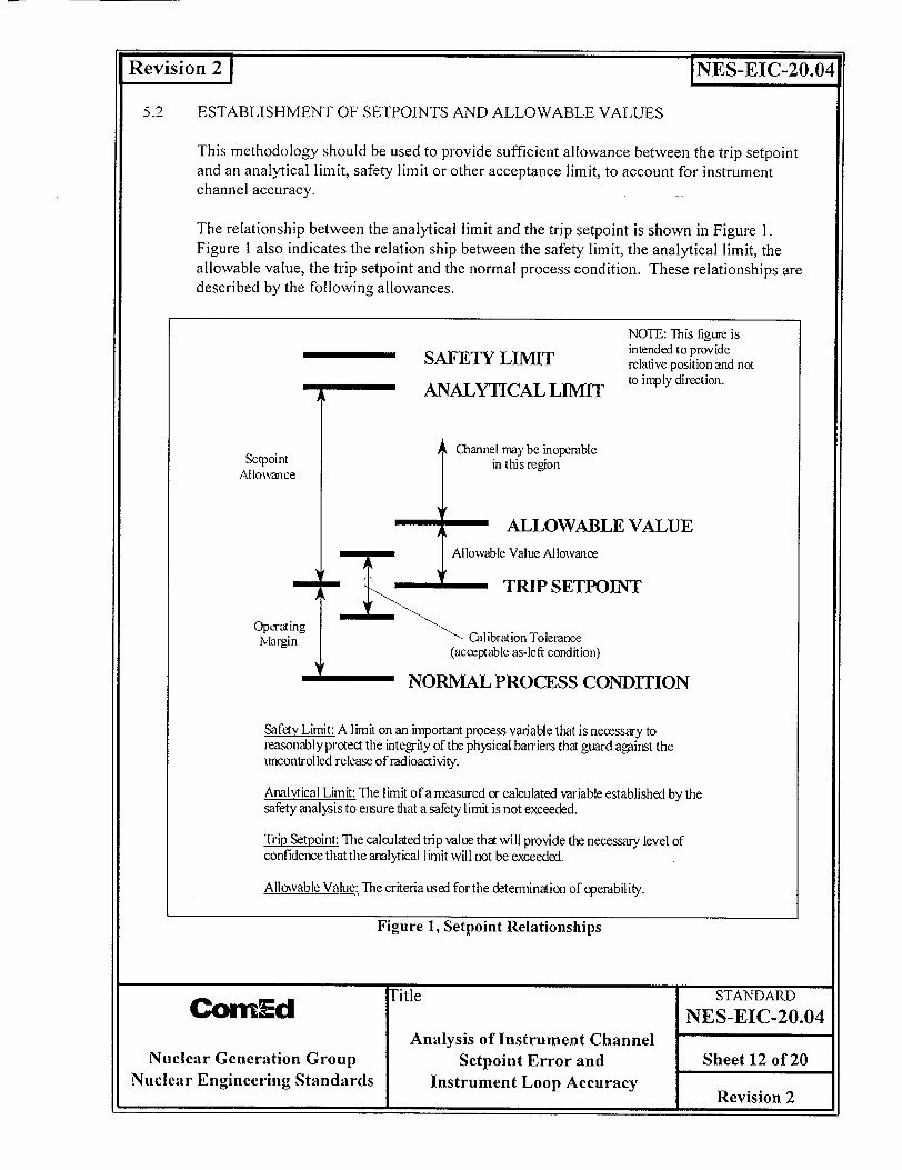
5.2 ESTABLISHMENT OF SETPOINTS AND ALLOWABLE VALUES
This methodology should be used to provide sufficient allowance between the trip setpoint and an analytical limit, safety limit or other acceptance limit, to account for instrument channel accuracy.
The relationship between the analytical limit and the trip setpoint is shown in Figure 1. Figure 1 also indicates the relation ship between the safety limit, the analytical limit, the allowable value, the trip setpoint and the normal process condition. These relationships are described by the following allowances.
SSAFETY LIMIT
ANALYTICAL LIMIT
NOTE: This figure is intended to provide relative position and not to imply direction.
Channel may be inoperable in this region
ALLOWABLE VALUE
SAllowable Value Allowance
n TRIP SETPOINT
ing in Calibration Tolerance
(acceptable as-left condition)
"NORMAL PROCESS CONDITION
Safetv Limit: A limit on an important process variable that is necessary to reasonably protect the integrity of the physical barriers that guard against the uncontrolled release of radioactivity.
Analytical Limit: The limit of a measured or calculated variable established by the safety analysis to ensure that a safety limit is not exceeded.
Trip Setpoint- The calculated trip value that will provide the necessary level of confidence that the analytical limit will not be exceeded.
Allowable Value: The criteria used for the determination of operability.
Figure 1, Setpoint Relationships
Title STANDARD Cbm•d NES-EIC-20.04 Analysis of Instrument Channel
Nuclear Generation Group Setpoint Error and Sheet 12 of 20 Nuclear Engineering Standards Instrument Loop Accuracy t) InRevision 2
eSetpoint
Allowanc
Operat Margi
A
j

p I
Revision 2 1 INES-EIC-20.04
5.2.1 Setpoint Allowance: The setpoint allowance describes the relationship between the trip setpoint and the analytical limit. This allowance may be determined through the evaluation of the instrument channel accuracy, operating experience (including as-found/asleft analysis), equipment qualification tests, vendor design specifications, engineering analyses, laboratory tests, engineering drawings, etc.
The setpoint allowance shall account for all applicable design basis events (normal and abnormal) and the following process instrument uncertainties unless they were included in the determination of the analytical limit.
Instrument uncertainties included in the setpoint allowance:
1) Instrumentation calibration uncertainties; including: * calibration standards, * calibration M&TE, and * setting tolerances.
2) Calibration methods 3) Instrument uncertainties during normal operation; including:
0 reference accuracy, * power supply voltage and frequency changes, * ambient temperature changes, * humidity changes, * pressure changes, * inservice vibration allowances, * radiation exposure, and 0 AID and D/A conversion.
4) Instrument drift 5) Uncertainties caused by design basis events 6) Process dependent effects 7) Calculation effects 8) Dynamic effects 9) Installation biases
It is often difficult to determine what errors and uncertainties have been included by the NSSS supplier or A/E in the determination of the original design basis analytical limit. This is especially true for the environmental conditions. It should not be assumed that analytical limits contained in ComEd documents and/or Tech Specs are correctly implemented as LSSS setpoints or calculated setpoints without evaluation of the original setpoint accuracy analysis or preparation of a new analysis using this standard.
Title STANDARD
COmEd NES-EIC-20.04
Analysis of Instrument Channel Nuclear Generation Group Setpoint Error and Sheet 13 of 20
Nuclear Engineering Standards Instrument Loop Accuracy Revision 2

Revisio n 2 1 INES-EIC-20.04
5.2.2 Allowable Value Allowance: This allowance describes the relationship between the trip setpoint and the allowable value. The purpose of the allowable value is to identify a value that, if exceeded, may mean that the instrument, device or channel has not performed within the basis of the setpoint calculation. A channel whose as-found condition exceeds the allowable value should be evaluated for operability, taking into account the setpoint calculation methodology.
At CornEd nuclear stations, non-reactor protection setpoints frequently have administrative limits, reportable tolerances or other station specific criteria to evaluate the as-found condition of a setpoint, calibration or operational test. Refer to ER-AA,-520, Instrument Performance Trending, for additional information associated with these limits.
Instrument uncertainties included in the Allowable Value allowance:
1) Instrument calibration uncertainties 2) Instrument uncertainties during normal operation 3) Instrument drift
5.2.3 Operating Margin: This allowance describes the relationship between the normal process condition and the trip setpoint. It is considered good practice to evaluate this relationship in order to determine the effect of normal operating transients on the trip setpoint. The operating margin may consider instrument channel accuracy, transient analysis, "allowance for spurious trip allowance", operating experience (including asfound/as-left analysis), equipment qualification tests, vendor design specifications, engineering analysis, laboratory tests, engineering drawings, etc.
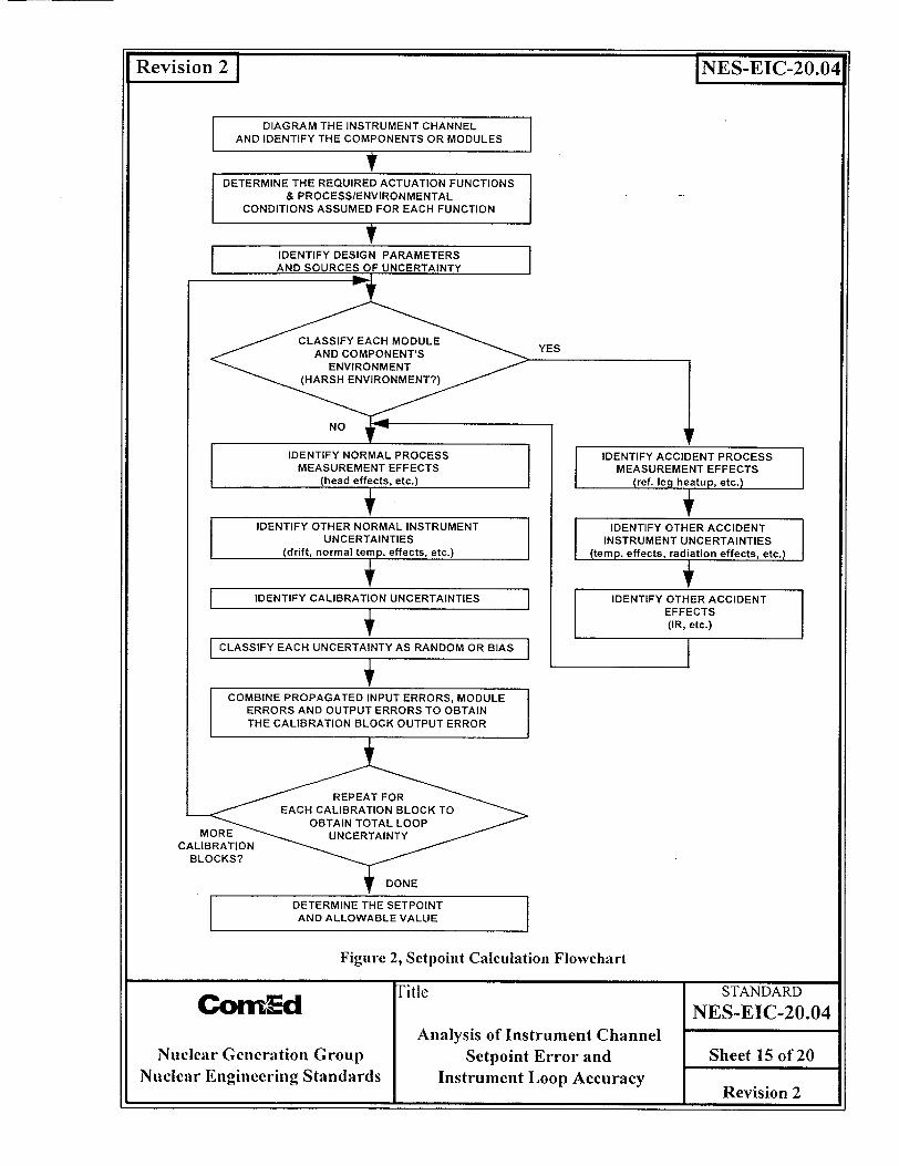
5.3 UNCERTAINTY ANALYSIS AND SETPOINT CALCULATION PROCESS
The process for determining instrument setpoints and allowable values is based on the analysis of the instrument loop accuracy and the identification of the acceptance criteria for each setpoint. This process is shown in figure 2.
5.3.1 Block Diagram the Instrument Channel and Identify Components, Modules and Calibration Blocks
The instrument channel to be analyzed should first be diagrammed to ensure that all errors and uncertainties affecting instrument channel accuracy are identified and correctly applied. The process for determining instrument channel accuracy is based on the propagation of errors and uncertainties through the instrument channel from the process to the final output, i.e. actuation or indication.
Title STANDARD
CornEd NES-EIC-20.04
Analysis of Instrument Channel Nuclear Generation Group Setpoint Error and Sheet 14 of 20
Nuclear Engineering Standards Instrument Loop Accuracy Revision 2
I I
Revision 2 1 INES-EIC-20.04
Figure 2, Setpoint Calculation Flowchart
Title STANDARD C•OrEd NES-EIC-20.04
Analysis of Instrument Channel Nuclear Generation Group Setpoint Error and Sheet 15 of 20
Nuclear Engineering Standards Instrument Loop Accuracy Revision 2
Revision 2 [NES-EIC-20.04
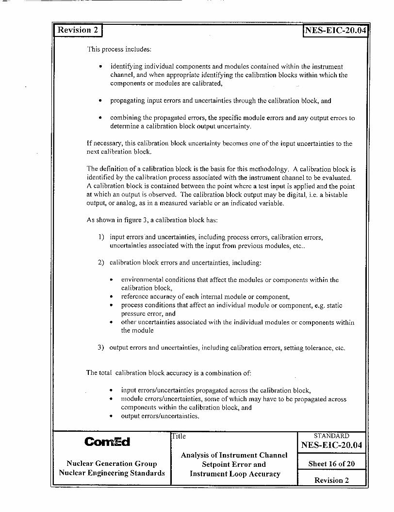
This process includes:
"• identifying individual components and modules contained within the instrument channel, and when appropriate identifying the calibration blocks within which the components or modules are calibrated,
"* propagating input errors and uncertainties through the calibration block, and
"* combining the propagated errors, the specific module errors and any output errors to determine a calibration block output uncertainty.
If necessary, this calibration block uncertainty becomes one of the input uncertainties to the next calibration block.
The definition of a calibration block is the basis for this methodology. A calibration block is identified by the calibration process associated with the instrument channel to be evaluated. A calibration block is contained between the point where a test input is applied and the point at which an output is observed. The calibration block output may be digital, i.e. a bistable output, or analog, as in a measured variable or an indicated variable.
As shown in figure 3, a calibration block has:
1) input errors and uncertainties, including process errors, calibration errors, uncertainties associated with the input from previous modules, etc..
2) calibration block errors and uncertainties, including:
* environmental conditions that affect the modules or components within the calibration block,
* reference accuracy of each internal module or component, * process conditions that affect an individual module or component, e.g. static
pressure error, and • other uncertainties associated with the individual modules or components within
the module
3) output errors and uncertainties, including calibration errors, setting tolerance, etc.
The total calibration block accuracy is a combination of:
"* input errors/uncertainties propagated across the calibration block, "* module errors/uncertainties, some of which may have to be propagated across
components within the calibration block, and "* output errors/uncertainties.
Title STANDARD CornEd NES-EIC-20.04 Analysis of Instrument Channel
Nuclear Generation Group Setpoint Error and Sheet 16 of 20 Nuclear Engineering Standards Instrument Loop Accuracy Revision 2
A Calibration Block Containing 1 or More Components or Modules
CALIBRATION BLOCK ERRORS - component/module errors and
uncertainties E errors and uncertainties from
INPUT ERRORS environmental effects
process errors component, module or loop drift
input measurement errors and uncertainties input calibration errors
OUTPUT ERRORS * propagated input errors o component/module errors
(these may require propagation)
* output calibration errors
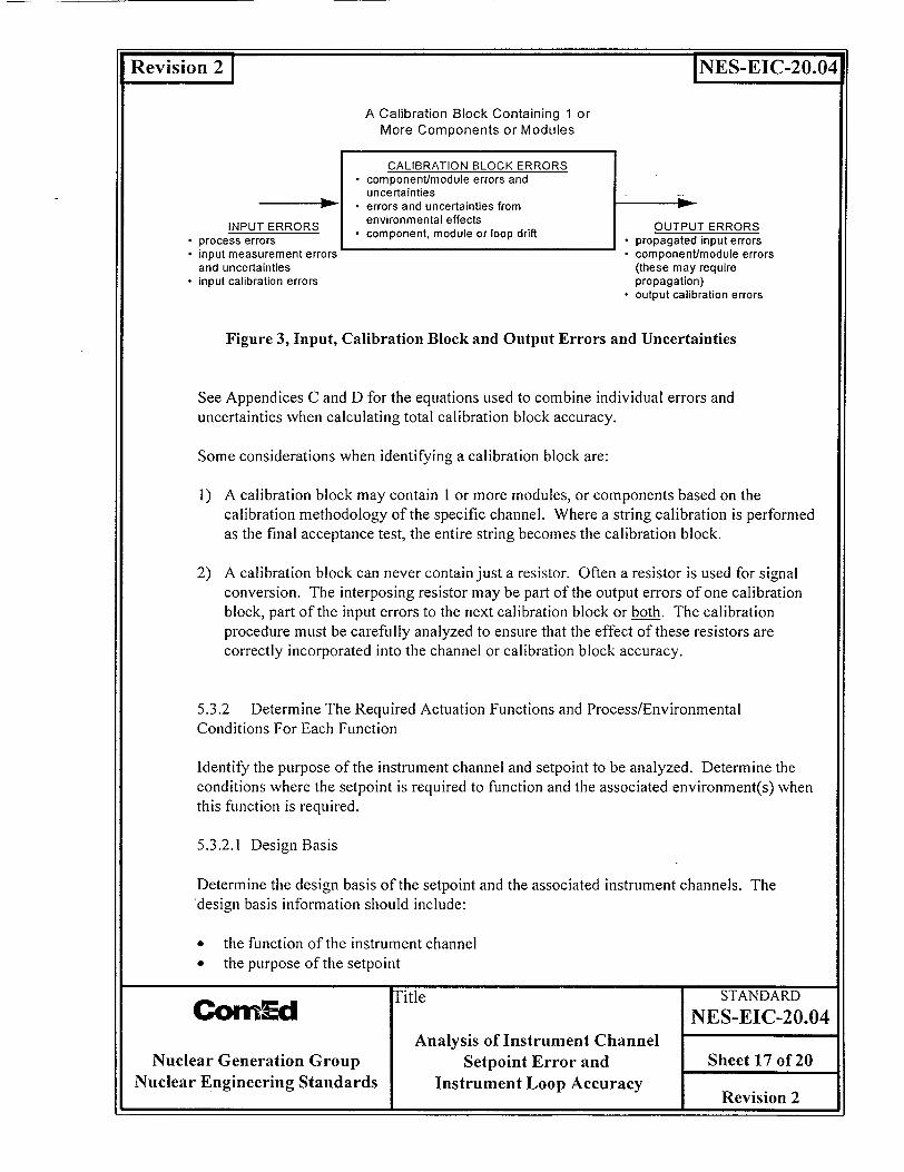
Figure 3, Input, Calibration Block and Output Errors and Uncertainties
See Appendices C and D for the equations used to combine individual errors and uncertainties when calculating total calibration block accuracy.
Some considerations when identifying a calibration block are:
1) A calibration block may contain 1 or more modules, or components based on the calibration methodology of the specific channel. Where a string calibration is performed as the final acceptance test, the entire string becomes the calibration block.
2) A calibration block can never contain just a resistor. Often a resistor is used for signal conversion. The interposing resistor may be part of the output errors of one calibration block, part of the input errors to the next calibration block or both. The calibration procedure must be carefully analyzed to ensure that the effect of these resistors are correctly incorporated into the channel or calibration block accuracy.
5.3.2 Determine The Required Actuation Functions and Process/Environmental Conditions For Each Function
Identify the purpose of the instrument channel and setpoint to be analyzed. Determine the conditions where the setpoint is required to function and the associated environment(s) when this function is required.
5.3.2.1 Design Basis
Determine the design basis of the setpoint and the associated instrument channels. The design basis information should include:
0
0
the function of the instrument channel the purpose of the setpoint
Title STANDARD COrn u NES-EIC-20.04
Analysis of Instrument Channel Nuclear Generation Group Setpoint Error and Sheet 17 of 20
Nuclear Engineering Standards Instrument Loop Accuracy Revision 2
Revision 2 1 INES-EIC-20.04
p
n 2 1 NES-EIC-20.04
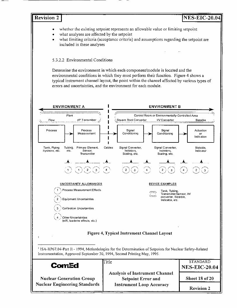
"* whether the existing setpoint represents an allowable value or limiting setpoint "* what analyses are affected by the setpoint "* what limiting criteria (acceptance criteria) and assumptions regarding the setpoint are
included in these analyses
5.3.2.2 Environmental Conditions
Determine the environment in which each component/module is located and the environmental conditions in which they must perform their function. Figure 4 shows a typical instrument channel layout, the point within the channel affected by various types of errors and uncertainties, and the environment for each module.
_d P T ra ns mitt e r•
ENVIRONMENT B
Control Room or Envi ronmentally-Controlled Area
,Square Root Converter IN Converter Bistable
Signal Signal Actuation Conditioning Conditioning or
Indication
Tank, Piping Tubing, Primary Element, Systems, etc. etc. Sensor,
Transmitter
A
Cables Signal Converter, Isolators,
Scaling, etc.
Signal Converter, Isolators,
Scaling, etc.
A
1 1 , 2 . 3 4
UNCERTAINTY ALLOWANCES
1 -. Process Measurement Effects
2"• Equipment Uncertainties
3 Calibration Uncertainties ,f
,4 'Other Uncertainties
"(eIR. leadwire effects, etc.)
2 3 4'
DEVICE EXAMPLES
, Tank, Tubing, Transmitter/Sensor, IA1 converter, Bistable, Indicator. etc.
Figure 4, Typical Instrument Channel Layout
ISA-RP67.04-Part I1 - 1994, Methodologies for the Determination of Setpoints for Nuclear Safety-Related
Instrumentation, Approved September 30, 1994, Second Printing May, 1995.
Title STANDARD ComEd NES-EIC-20.04
Analysis of Instrument Channel Nuclear Generation Group Setpoint Error and Sheet 18 of 20
Nuclear Engineering Standards Instrument Loop Accuracy I f_ý ý I I Revision 2
ENVIRONMENT A
Plant
Flow
Bistable, Indicator
2 4 2 ~3
h2:!sion�fl I NES-EIC-20.04
5.3.3 Identify Design Parameters and Sources of Uncertainty
Once the design basis for the instrument setpoint and environment is determined, identify the potential sources of errors and uncertainties that may affect the instrument channel accuracy.
See Appendix A for a discussion of the minimum list of errors and uncertainties that must be included in accordance with this standard. This minimum list is not intended to limit the types and sources of error and uncertainty associated with an instrument setpoint. Each instrument channel, method of process measurement, calibration methodology, and environment may have unique errors and uncertainties.
5.3.4 Classify Each Modules Environment
This standard requires that the station specific EQ Zones contained in the UFSAR and the station specific environmental conditions associated for each zone are to be used in evaluating all environmental effects.
5.3.5 Identify Normal/Accident Process Measurement Effects, Instrument Uncertainties, Calibration Uncertainties and Other Uncertainties, and Classify Each Uncertainty as Random, Bias, etc.
See Appendix A and Reference 3.2 for applicable error effect equations and methods for determining values of uncertainty.
5.3.6 Combine Propagated Input Errors, Module Errors and Output Errors to Yield Total Calibration Block Output Error
See Appendix B for error propagation and Appendix C for equations for the combination of errors and uncertainties.
5.3.7 Obtain Total Channel Uncertainty
See appendix C for the methodology and equations used to combine individual errors and uncertainties.
Title STANDARD COr uEd NES-EIC-20.04
Analysis of Instrument Channel Nuclear Generation Group Setpoint Error and Sheet 19 of 20
Nuclear Engineering Standards Instrument Loop Accuracy Revision 2
INES-EIC-20.04Revision 2 1

�sio23J NES-EIC-20.04
5.3.8 Determine the Setpoint and Allowable Value
See appendix C for the methodology and equations used to determine an instrument setpoint and an associated allowable value.
5.3.9 Administrative Limits
Refer to ER-AA-520, Instrument Performance Trending, when administrative limits are required as part of the instrument loop accuracy determination.
"Title STANDARD COrn [ NES-EIC-20.04
Analysis of Instrument Channel Nuclear Generation Group Setpoint Error and Sheet 20 of 20
Nuclear Engineering Standards Instrument Loop Accuracy Revision 2
Revision 2 1 INES-EIC-20.04
I
I,Revision 2 INES-EIC-20.04
APPENDIX A
SOURCES OF ERROR AND UNCERTAINTY
Latest Revision indicated by a bar in right hand margin. .
Title STANDARD GomEd NES-EIC-20.04
Analysis of Instrument Channel APPENDIX A
Nuclear Operations Division Setpoint Error and Sheet Al of A16 Nuclear Engineering Standards Instrument Loop Accuracy Revision 2

tevision2 INES-EIC-20.04
This appendix discusses the sources of error that may affect instrument loop accuracy. In all cases, sound engineering judgment should be applied to account for errors not explicitly described below. Significant errors, whether or not they are described in this appendix shall also be included in the computation of setpoint error, or instrument loop accuracy.
This appendix provides a minimum list of errors and uncertainties that shall be evaluated for each component and module when evaluating instrument channel accuracy in accordance with this standard.
1.0 PROCESS ERRORS
Process errors result from changes in the process or sensing channel from the nominal, or calibration conditions. They may also result from conditions that cannot be readily measured, e.g. turbulence or other system complexities To account for process errors in a setpoint error calculation, it is necessary to model the process, and the effects of sensing elements on the process. For example, intrusive flow sensing devices, such as venturis, directly effect the process that they measure. Process models should account for calibration conditions, normal operation, and accident conditions. For each of these conditions, the behavior of all applicable process variables, such as temperature, pressure, and density, must be understood well enough to predict the error.
Changes in the process may result in either random or non-random errors. Non-random process errors are those which can predictably be correlated to process conditions, such as thermal expansion effects. Random errors result from uncertainties that are not predictable as to their direction, but exist as a range or limit of error around the process value.
1. 1 DENSITY EFFECTS
Measurements of fluid flow, pressure, and levels are effected by the process densities. Density changes in the process and in instrument sensing lines can result in measurement errors. An example of a process measurement that is affected by density changes is the measurement of fluid flow. Fluid flow is inversely proportional to the square root of fluid density. If a flow meter is calibrated for a specific fluid density, and the density changes, then a flow measurement error that is inversely proportional to the square root of the density change will result.
1.2 FLOW ERRORS
Flow measurements are based on nominal values for the dimensions of components such as nozzles, orifices, and venturis. These devices are subject to changes in dimension due to the erosion and/or corrosion effects of the material they contain. Changes in pipe diameter, or
"M Title STANDARD
COrn d NES-EIC-20.04 Analysis of Instrument Channel APPENDIX A
Nuclear Operations Division Setpoint Error and Sheet A2 of A16 Nuclear Engineering Standards Instrument Loop Accuracy Revision 2
p
Revision 2 [NES-EIC-20.04
bore tolerance will cause flow measurement errors. and should be considered in the evaluation of instrument loop accuracy
1.3 TEMPERATURE ERRORS
Changes in the process media temperature from the nominal or calibration values will cause process measurement errors. Pressure and differential pressure measurements are particularly susceptible to temperature induced errors. Pressure and level measurements are made by sensing the hydrostatic head pressure of a fluid. The hydrostatic head pressure of a fluid is directly proportional to the product of the fluid's height and specific weight. Since specific weight is a temperature dependent parameter, temperature changes in the process fluid will cause process measurement errors. Temperature induced process errors will affect pressure, level, and flow measurements and should be considered in the evaluation of instrument loop accuracy.
1.4 THERMAL EXPANSION ERRORS
Changes in temperature cause dimensional changes in system structures, components and instrument sensing lines. Instrument calibration is often based on specific sensing line or component installed elevations. Component elevation changes due to temperature effects will cause process measurement errors and should be considered in the evaluation of instrument loop accuracy.
An example of a thermal expansion effect on a process measurement is reactor pressure vessel growth. As the reactor is heated and pressurized to operating conditions, dimensional increases occur. Differential pressure level sensing instruments are calibrated for specific values of process tap and component elevations. These elevations may change from calibration values as the reactor is brought tip to operating conditions as a result of thermal expansion.
Thermal expansion errors should be accounted for in the evaluation of instrument loop accuracy.
1.5 PIPING CONFIGURATION
Intrusive devices, i.e. nozzles, orifices, venturis and valves, as well as pipe bends, changes in pipe diameter and material cause turbulence in flow media. Flow turbulence is a source of flow measurement error. Inspection of piping and isometric drawings can provide information on the proximity of flow sensors to fittings and valves that cause turbulence. It may be possible to bound flow measurement error due to turbulence based on the upstream
"M -d Title STANDARD Cam = NES-EIC-20.04
Analysis of Instrument Channel APPENDIX A Nuclear Operations Division Setpoint Error and Sheet A3 of A16
Nuclear Engineering Standards Instrument Loop Accuracy Revision 2

Revision 2NES-EIC-20.04
or downstream separation between the flow sensor and source of turbulence. Refer to References 3.2, 3.10 and 3.13 for additional information.
2.0 REFERENCE ACCURACY (RA)
The Reference Accuracy of an instrument loop component is never zero. This would infer that there is no difference between the true value of a process and the measured value of a process. Error free measurements are physically impossible.
The error due to the Reference Accuracy of an instrument is usually given as a numerical expression, graph, or specification published by the instrument vendor.
Where independent test labs rather than the manufacturers have evaluated an instrument's performance characteristics, the test methods should be reviewed to ensure that the test results are consistent with their intended use.
The error due to instrument Reference Accuracy is classified as a normally distributed random variable.
3.0 OPERATIONAL ERRORS.
3.1 Drift (D)
Instrument drift is a change in instrument performance that occurs over a period of time that is unrelated to input, environment or load. Drift independently effects all components of an instrument loop. Ambient conditions such as temperature, radiation, and humidity do not affect the magnitude of an instrument's drift.
Specific instrument drift effect data is typically provided from: "* The instrument manufacturer "* The review of historical calibration data "• Documentation industry experience "* Environmental Test Reports
If specific values for this effect are not available from these sources, the following default values may be included when preparing the analysis for additional conservatism. The CornEd default drift effect values that will be used in these cases are:
Mechanical Components: +1.0% of span per refueling cycle Electronic Components: +0.5% of span per refueling cycle
"M -M fitle STANDARD GCNt~d NES-EIC-20.04
Analysis of Instrument Channel APPENDIX A
Nuclear Operations Division Setpoint Error and Sheet A4 of A16 Nuclear Enginecring Standards Instrument Loop Accuracy
I t, I I Revision 2
Revision 2 1 INES-EIC-20.04
The intent of these CornEd default drift effect values is to establish consistent values for this type of error for inclusion into the calculations to achieve additional conservatism when this data is not available, applicable, or published. Selection of these default drift effect values is the result of engineering review and judgement of industry practices, typical Reference Accuracy for these device types, and industry experience. These default drift effect values shall not be used when instrument drift effect data is available from the sources listed above.
Manufacturer's published "drift specifications" that are explicitly dependent on operational conditions, i.e. temperature, should not be misinterpreted as Drift in the instrument analysis. In these instances, the use of the word drift is inconsistent with the definition in this standard. An example of this is, "the instrument's zero drift is 10 mv/ C." The net effect of drift on the components of an actuating loop may shift the trip point in the conservative direction, the non-conservative direction, or not at all. Drift is probabilistic in nature. Therefore, the magnitude and direction of its effects are impossible to predict precisely.
Drift is classified as a symmetric random error. This classification accurately models the uncertainty in the sign of the drift error and assumes that the maximum possible drift always occurs between successive instrument surveillances. However, if a instrument surveillance occurs either before or after the manufacturer's published drift interval, then the value for drift must be adjusted to account for the differing intervals (see Eq. Al or A2).
Where the error caused by drift is assumed to be a linear function of time, equation Al should be used. If the engineer preparing the calculation determines that the drift effect is not a linear function, i.e. "point drift", then the basis for the drift function shall be explained in the calculation.
The following equation should be used to calculate instrument drift (D):
D = (I +LF/SI)SIxIDE (Eq. Al)
where: IDE = instrument drift effect that is specified by the instrument vendor, published
by an independent test lab, or determined from plant historical data.
SI = instrument surveillance interval specified in the station technical specifications or other station document.
LF = test interval late factor. This is the amount of time (grace period) by which a required instrument surveillance is administratively allowed to exceed the licensed surveillance period. Surveillance intervals, grace periods and Late Factor are found in the plant technical specifications.
FE Title STANDARD
~Ownc NES-EIC-20.04 Analysis of Instrument Channel APPENDIX A
Nuclear Operations Division Setpoint Error and Sheet A5 of A16 Nuclear Engineering Standards Instrument Loop Accuracy
rRevision 2
Revision 2 1 INES-EIC-20.04
This method of drift error calculations should be used unless other data or vendor information is available. The drift term is considered a linear function of time unless other methods to evaluate drift are available.
Where multiple time periods of IDE and/or SI are to be evaluated, and it can be shown or reasonably argued that the drift error during each drift period is random and independent, then the SRSS of the individual drift periods between calibrations may be used.
D = [ IDE ] [(SI+LF)/VDP]1/2 (Eq. A2)
where: VDP = vendor drift period that is specified by the instrument vendor or obtained
from other testing (e.g. as-found/as-left analysis).
Example: SI+LF = 22 V2 months VDP = 12 months IDE = 1% span per 12 month period
1/2 D=[1%][22 1/2/ 12] =±l.37% span
3.2 STATIC PRESSURE EFFECTS (eSP)
Static pressure effects are instrument errors due to a change in process pressure from the value present at the time of calibration. These effects should be considered for those devices with sensing elements that are in direct contact with the process. This effect typically applies to differential pressure sensors.
eSP = ISPE(ASP) (Eq. A3)
where: ISPE = the instrument static pressure effect specified by the vendor, independent
test lab or determined from plant historical data.
ASP = the changes in static pressure conditions from calibration conditions.
3.3 PRESSURE EFFECTS (eP)
Pressure changes can cause density changes in process media. Pressure induced density changes in process media from nominal or calibration values are sources of process measurement error. Pressure changes due to environmental or accident effects can cause measurements errors in process parameters.
Title STANDARD CornEd NES-EIC-20.04
Analysis of Instrument Channel APPENDIX A
Nuclear Operations Division Setpoint Error and Sheet A6 of A16 Nuclear Engineering Standards Instrument Loop Accuracy Revision 2

Revision 2 J INES-EIC-20.04
eP = IPE(AP) (Eq. A4)
where: IPE = instrument pressure effect is determined from vendor specifications, pub
lished independent test lab data or plant historical data.
AP = changes in pressure from calibration conditions.
3.4 POWER SUPPLY EFFECTS (eV)
Variations in the output of an instrument loop's power supply may cause errors in process measurement. Instrument errors due to fluctuations in the loop power supply may be estimated by:
eV = IPSE(AV) (Eq. A5)
where: IPSE = Instrument power supply effect is determined from vendor specifications or
published independent test lab data.
AV = power supply stability as determined from plant data
4.0 ENVIRONMENTAL ERRORS
Changes in environmental conditions from those present at the time of calibration can cause measurement errors. Errors due to environmental fluctuations can occur during calibration, during normal operation, or during an accident and should be included in the calculation of instrument loop accuracy.
Environmental errors are classified as non-random. The following three methods may be used to specify environmental error effects.
1) A numerical constant that bounds the error is specified for a specific range of environmental conditions. This constant is specified by the instrument manufacturer, or an independent test lab. An example of this type of error specification is:
1% of output span for ambient temperatures of 60 -.90'F.
2) An instrument's environmental error is calculated by evaluating a model that describes the instruments sensitivity to specific environmental fluctuations. Environmental error models may be available from instrument manufacturers and published in the
Title STANDARD CornEd NES-EIC-20.04
Analysis of Instrument Channel APPENDIX A Nuclear Operations Division Setpoint Error and Sheet A7 of A16
Nuclear Engineering Standards Instrument Loop Accuracy Revision 2

Revision 2
instrument specifications, or from independent test labs. An example of this type of error specification is:
Temperature Error (eT) = 0.75% of the Upper Range Limit + 0.50% of the Calibrated Span
3) An instrument's environmental errors may be given as a graphical specification. Figure Al shows a graphical representation of instrument error based on empirical or calculated data gathered by the instrument manufacturer, or by an independent test lab. A graphical error specification shows instrument error as a function of environmental changes.
a. 2.4 2.2
S2.0
1.6
,2 1.4o 1.2
1.0
S0.8W- 0.6
,• 0.4
> 0.2
0 30 50 70 90 110 130
Temperature (fF)
Figure Al, Graphical Specification of Device Error
4.1 TEMPERATURE EFFECTS (eT)
Temperature errors result from deviations in ambient temperature at the instrument location from the temperature at which the instrument was previously calibrated. Where a mathematical model (ITE) is available for temperature error, then the model should be evaluated for the anticipated temperature change.
eT = ITE(AT) (Eq. A6)
where: ITE = the instrument temperature effect that models the measurement error as a
function of the temperature changes (AT).
4.2 HUMIDITY EFFECTS (eH)
i Title STANDARD COMMd NES-EIC-20.04
Analysis of Instrument Channel APPENDIX A
Nuclear Operations Division Setpoint Error and Sheet A8 of A16 Nuclear Engineering Standards Instrument Loop Accuracy Revision 2
INES-EIC-20.04
Revision 2 1- I
INES-EIC-20.04
Humidity errors are due to changes in humidity at an instrument location from calibration or nominal values. If a model is available for humidity error, then the model should be evaluated for the anticipated humidity change.
eH = IHE(AH) (Eq. A7)
where: IHE = the instrument humidity effect that models the measurement error as a
function of humidity changes (AH).
4.3 RADIATION EFFECTS (eR)
Radiation errors are caused by instrument exposure to ionizing radiation. If a model is available for radiation error, then the model should be evaluated for the anticipated radiation dose.
eR = IRE(TID) (Eq. A8)
where: IRE = the instrument radiation effect that models the measurement error as a
function of radiation dose, expressed as total integrated dose (TID).
4.4 SEISMIC EFFECTS (eS)
Seismic errors result from subjecting an instrument to high energy vibrations and accelerations. If a model is available for seismic error, then that model should be evaluated for the anticipated acceleration at the instrument location.
eS = ISE(ZPA)
where: ISE =
(Eq. A9)
the instrument seismic effect that models the measurement error as a function of Zero Period Acceleration (ZPA) anticipated at the instrument location.
Seismic error models must take into account the instrument response due to location, mounting, orientation, and flexibility of the instrument, etc. Data for required response spectra and the associated error due to seismic effects should be obtained from the plant .UFSAR, seismic test reports, and seismic structure analysis reports. The published instrument error (and its associated ZPA due to seismic effects should be compared with the required response spectrum specified for the instrument location to ensure that they are consistent. IEEE Recommended Practice For Seismic Qualification of Class I E Equipment
no Title STANDARD CornEd NES-EIC-20.04
Analysis of Instrument Channel APPENDIX A Nuclear Operations Division Setpoint Error and Sheet A9 of A16
Nuclear Engineering Standards Instrument Loop Accuracy 1 f1 1 1 Revision 2

Revision 2 ]NES-EIC-20.04
For Nuclear Power Generating Stations (reference 3.18) defines Required Response Spectrum (RRS) as, "The response spectrum issued by the user or his agent as part of his specifications for qualifications or artificially created to cover future applications. The RRS constitutes a requirement to be met".
5.0 CALIBRATION ERRORS
Errors that occur in the adjustment and measurement of loop element signals due to measurement and test equipment (M&TE) are called calibration errors. Calibration errors are classified as random and include:
"* M&TE reference accuracy,
"* M&TE reading error,
"* M&TE environmental errors,
"* calibration standard reference accuracy (STD),
"* calibration standard reading error, and
"* setting tolerance (ST).
5.1 MEASUREMENT AND TEST EQUIPMENT (M&TE).
5.1.1 M&TE Error (RAMTE)
All calibration procedures require measurement and test equipment to monitor instrument adjustments using a specified set of conditions. Some calibration procedures require additional test components whose accuracy must be included in the determination of calibration error. M&TE error includes the reference accuracy of each device, the uncertainties resulting from the environment in which the M&TE was calibrated or used, and the uncertainty added by any component used in a calibration procedure. M&TE accuracy should be obtained from the manufacturer's published specifications unless the device has been calibrated or maintained to a different set of criteria. At ComEd, the calibration facility may be directed to maintain the M&TE to a accuracy different from the manufacturer's specification. This difference should be documented in the basis for the- M&TE accuracy used in the instrument channel or setpoint accuracy calculation. When assumptions are
-required regarding which particular M&TE device may be utilized in a test or calibration procedure, the assumed accuracy of the test equipment data should be equal to that of the least accurate instrument in the group of possible candidates.
" E Title STANDARD
Corn~d NES-EIC-20.04
Analysis of Instrument Channel APPENDIX A Nuclear Operations Division Setpoint Error and Sheet A10 of A16
Nuclear Engineering Standards Instrument Loop Accuracy Revision 2
Revision 2 1 INES-EIC-20.04
Measurement and test equipment used during calibration procedures may be sensitive to environmental fluctuations. M&TE errors should use the largest expected change between the instrument calibration conditions and the normal environment. These extremes typically are obtained from EQ documents, e.g. the station EQ zone maps. This provides a bounding or conservative estimate of M&TE environmental error. Restricting or assuming that the calibration environment deviates less than the associated EQ zone is not desirable since it places added requirements on the IM's to document the assumed environmental condition during each calibration.
5.1.2 Reading Error (REMTE)
Since it is unlikely that an analog gauge reading will always coincide with a graduation tick mark, the readability of the gauge scale is ½ of the smallest division. The uncertainty in this readability, or reading error (RE), is ± '/4 of the smallest graduation interval. For devices that have non-linear scales, the division used to determine the reading error is consistent with the desired reading.
For digital output devices, the reading error is considered to be the least significant digit (LSD) or least significant increment of the display.
5.1.3 Input M&TE Temperature Error (TEMTE)
M&TE temperature errors are determined from the vendor's expression for temperature effects (ITE) and the range of temperature fluctuations (AT). The temperature extremes at which the M&TE equipment was calibrated and the ambient temperature extremes in which the M&TE device is going to be used should be evaluated.
5.1.4 Calibration Standard Error (STD).
Calibration standards are used to perform periodic calibrations on M&TE. If the calibration standard is at least 4 times more accurate than the M&TE, then its error represents at most 6.25% of the M&TE error, and may be assumed to be negligible. If the calibration standard is not 4 times more accurate than the measurement and test equipment, then its error should be factored into the calculation of calibration error. Refer to NES-EIC-20.01, Standard for Evaluation of M&TE Accuracy When Calibrating Instrument Components and Channels, for additional guidance.
5.1.5 Surveillance Interval (SI).
Title STANDARD COrnEd NES-EIC-20.04
Analysis of Instrument Channel APPENDIX A
Nuclear Operations Division Setpoint Error and Sheet All of A16 Nuclear Engineering Standards Instrument Loop Accuracy Revision 2
Revision 2 1 INES-EIC-20.04
The surveillance interval is the period between successive instrument surveillances or calibrations. Surveillance intervals are specified in the plant technical specifications, implemented in the plant calibration procedures, or identified by station instrument calibration scheduling programs.
Station Technical Specifications may allow a grace period beyond the specified calibration frequency. The surveillance frequency is typically limited to 125% of the required SI. The grace period should be included in the determination of instrument loop accuracy. The grace period should not be included in the calculation of the Allowable Value since it results in the potential for non-conservative evaluation of operability.
5.2 SETTING TOLERANCE (ST)
Setting tolerance is the uncertainty associated with the calibration procedure allowances used by technicians in the calibration process. Programs exist at each station to ensure that instrument channels and calibrated setpoints will not be left outside of a specified setting tolerance. As a result, it is expected that 100% of the population is left within the required setting tolerance. For pre-existing instrument channels that have established calibration procedures, the setting tolerance should be incorporated into the setpoint calculation as a 3)( error estimate. For new channels, the setting tolerance should be conservatively determined to justify a 3ca confidence value.
6.0 CALCULATIONAL ERRORS
6.1 NUMERICAL PRECISION AND ROUNDING
The precision of a number is determined by the significant digits in the number. Conclusions based on a calculation or measurement depend on the number of significant digits in the result of the calculation, or measurement. Calculated results can be no more precise than the calculation input data. To prevent the propagation of rounding and truncation errors in a calculation, round only the final result.
The final result should be rounded to the numnber ofsignificant digits found in the least precise input data but no less than the number of significant digits utilized in presenting the calibration setpoint or the calibration endpoints for loops that do not have setpoints. If the output is read on a DVM that displays 3 digits after the decimalpoint, the calculations conclusions must be rounded to no less than 3 digits after the decimal point.
This standard recommends the following method for rounding. The left-most non-zero digit in a number is the most significant digit. The right-most non-zero digit is the least sionificant digit if there is no decimal point. If there is a decimal point, the right most digit
Title STANDARD CornEd NES-EIC-20.04
Analysis of Instrument Channel APPENDIX A
Nuclear Operations Division Setpoint Error and Sheet A12 of A16 Nuclear Engineering Standards Instrument Loop Accuracy Lý I F Revision 2

Revision 2 1 INES-EIC-20.04is the least significant digit. The number of digits between the most significant and least significant digits are counted as the number of significant digits associated with a calculation, or measurement. The following numbers all have 4 significant digits: 1234, 1.234, 10. 10, 0.0001010, 1.000 e-4.
Round the final results of calculations to a level of precision that is consistent with the data input to the calculation. The rules for rounding are:
1. If the next digit less than the desired degree of precision is greater than 5, round up the least significant digit.
Example: 1.2347 = 1.235
2. If the next digit less than the desired degree of precision is less than 5, do not change the least significant digit.
Example: 7.8932 = 7.893
3. If the next digit less than the desire degree of precision is equal to 5, increment the least significant digit only if it is an odd number.
3.4325 = 3.432, 3.4335 z 3.434
6.2 A-D AND D-A ERRORS
Analog-to-Digital or Digital-to-Analog conversions (A/D or D/A) errors occur whenever a continuous process is represented digitally with a fixed number of bits. The resolution of the A/D or D/A converter is a primary consideration when evaluating A/D or D/A errors. Resolution is given by:
Resolution - (1/2")(signal span)
where 'n' is the number of bits in the A/D or D/A converter and signal span is the signal range present at the input of the A/D or D/A converter. There are several types of A/D or D/A converters, each of which has different sources of conversion error. Therefore, other A/D or D/A conversion errors must be determined on a case-by-case basis.
7.0 INSULATION RESISTANCE ERROR (eIR)
The eIR error shall be evaluated for all instrument components and instrument modules where the actuation function is expected to operate in an abnormal or harsh environment.
Title STANDARD
CornEd NES-EIC-20.04
Analysis of Instrument Channel APPENDIX A Nuclear Operations Division Setpoint Error and Sheet A13 of A16
Nuclear Engineering Standards Instrument Loop Accuracy Revision 2
Examples:
Revision 2 1 INES-EIC-20.04
Sources of data for insulation resistance should include values typical for the instrument loop tinder consideration, such as maximum supply voltage, nominal supply voltage, maximum loop resistance, minimum loop resistance, nominal insulation resistance (which should include conductor-to-conductor and conductor-to-ground values), and splice and terminal block insulation resistance. It may be necessary to arrive at these values through performance of generic calculations typical of several types of instrument loops. For a further effects of process measurement errors due to accident related insulation resistance degradation see Reference 3.2.
8.0 Setpoint Margin (MAR)
Margin may be included in the determination of instrument loop accuracy when an additional level of confidence is desired. For example, a particular vendor's testing methodology is not considered sufficiently rigorous to justify a 2cG confidence value for one of the published performance criteria. This determination may be based on engineering judgment, evaluation of the vendor's test plan or station/industry experience with the component. For the component in this example, it is determined that no other information exists to identify an alternate confidence level. This standard recommends that the vendor data should be incorporated at the 2u confidence level. Then an additional margin value is included in the instrument loop accuracy equation to provide additional conservatism.
NOTE: where as-found/as-left analysis or special test data is available, the component performance data should be utilized at the confidence level obtained fromn the statistical evaluation of the data.
For new instrument channels, an additional margin of 0.5% of the instrument measurement span, in instrument units, shall be included in order to account for unanticipated, or unknown loop component uncertainties. This margin may be deleted after sufficient calibration history exists to justify the instrument channel accuracy based on all other errors and uncertainties.
9.0 CLASSIFICATION OF ERROR TERMS
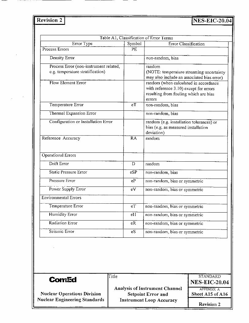
All errors and uncertainties shown in Table Al shall be evaluated as part of the determination of instrument loop accuracy. Where an individual error or uncertainty is 0, negligible or not applicable, the calculation shall describe why this condition is appropriate. Table I indicates the default classification for each type of error or uncertainty. These classifications may be changed as a result of published vendor information, other monitoring .programs (e.g. as-found/as-left drift analysis), or engineering judgment. The basis for any changes to the classification of an error term shall be fully documented in the associated instrument channel or setpoint accuracy calculation.
Title STANDARD
CornEd NES-EIC-20.04 Analysis of Instrument Channel APPENDIX A
Nuclear Operations Division Setpoint Error and Sheet A14 of A16
Nuclear Engineering Standards Instrument Loop Accuracy Revision 2
Revision 2 1 INES-EIC-20.04
Table Al, Classification of Error TermsError Type Symbol Error Classification
Process Errors PE
Density Error non-random, bias
Process Error (non-instrument related, random e.g. temperature stratification) (NOTE: temperature streaming uncertainty
may also include an associated bias error) Flow Element Error random (when calculated in accordance
with reference 3.10) except for errors resulting from fouling which are bias errors
Temperature Error eT non-random, bias
Thermal Expansion Error non-random, bias
Configuration or Installation Error random (e.g. installation tolerances) or bias (e.g. as measured installation deviation)
Reference Accuracy RA random
Operational Errors
Drift Error D random
Static Pressure Error eSP non-random, bias
Pressure Error eP non-random, bias or symmetric
Power Supply Error eV non-random, bias or symmetric
Environmental Errors
Temperature Error eT non-random, bias or symmetric
Humidity Error eH non-random, bias or symmetric
Radiation Error eR non-random, bias or symmetric
Seismic Error eS non-random, bias or symmetric
MM -0 Title STANDARD cem~u NES-EIC-20.04
Analysis of Instrument Channel APPENDIX A
Nuclear Operations Division Setpoint Error and Sheet A15 of A16 Nuclear Engineering Standards Instrument Loop Accuracy 6 eýI_ F Revision 2
I -
Revision 2 1 INES-EIC-20.04
Title STANDARD COwnEd NES-EIC-20.04
Analysis of Instrument Channel APPENDIX A Nuclear Operations Division Setpoint Error and Sheet A16 of A16
Nuclear Engineering Standards Instrument Loop Accuracy Revision 2
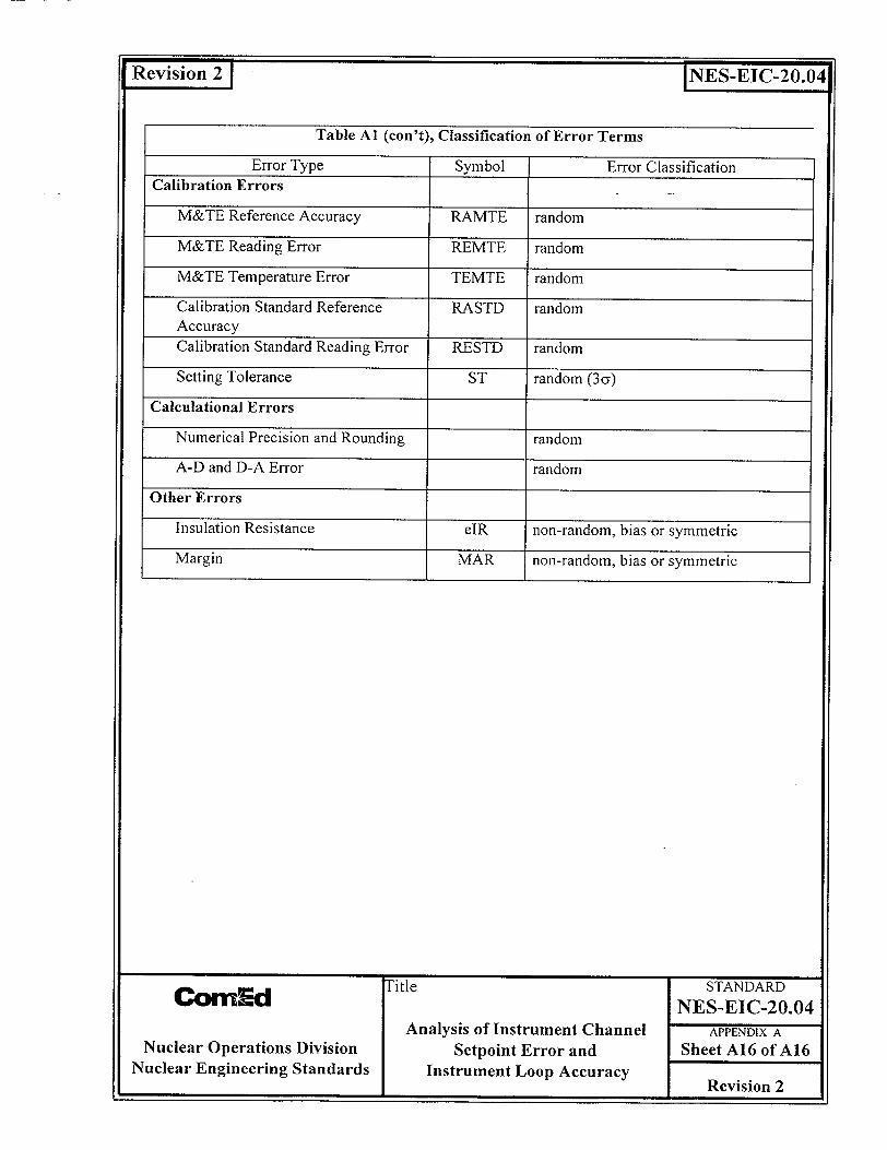
Table Al (con't), Classification of Error Terms
Error Type Symbol Error Classification Calibration Errors
M&TE Reference Accuracy RAMTE random
M&TE Reading Error REMTE random
M&TE Temperature Error TEMTE random
Calibration Standard Reference RASTD random Accuracy Calibration Standard Reading Error RESTD random
Setting Tolerance ST random (3 )
Calculational Errors
Numerical Precision and Rounding random
A-D and D-A Error random
Other Errors
Insulation Resistance eIR non-random, bias or symmetric
Margin MAR non-random, bias or symmetric
�sio�3J NES-EIC-.20.04
APPENDIX B
PROPAGATION OF ERROR AND UNCERTAINTIES
Latest Revision indicated by a bar in right hand margin.
Title STANDARD COrMn1 NES-EIC-20.04
Analysis of Instrument Channel APPENDIX B
Nuclear Generation Group Setpoint Error and Sheet B1 of B7 Nuclear Engineering Standards Instrument Loop Accuracy Revision 2
Reiso ,
Revision 2 1 INES-EIC-20.04
I I
Revision 2
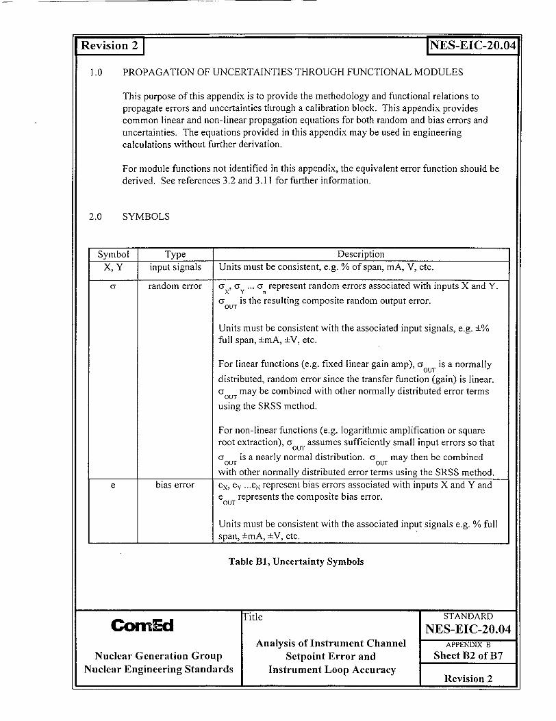
1.0 PROPAGATION OF UNCERTAINTIES THROUGH FUNCTIONAL MODULES
This purpose of this appendix is to provide the methodology and functional relations to propagate errors and uncertainties through a calibration block. This appendix provides common linear and non-linear propagation equations for both random and bias errors and uncertainties. The equations provided in this appendix may be used in engineering calculations without further derivation.
For module functions not identified in this appendix, the equivalent error function should be derived. See references 3.2 and 3.11 for further information.
2.0 SYMBOLS
Symbol Type Description X, Y input signals Units must be consistent, e.g. % of span, mA, V, etc.
CY random error CYx, a ... -a, represent random errors associated with inputs X and Y.
CY is the resulting composite random output error. OUTZ:
Units must be consistent with the associated input signals, e.g. ±% full span, ±mA, ±V, etc.
For linear functions (e.g. fixed linear gain amp), cy is a normally C:ý OUT
distributed, random error since the transfer function (gain) is linear. CYOUT may be combined with other normally distributed error terms
using the SRSS method.
For non-linear functions (e.g. logarithmic amplification or square root extraction), cy assumes sufficiently small input errors so that
(YOUT is a nearly normal distribution. cyOUT may then be combined with other normally distributed error terms using the SRSS method.
e bias error ex, ey ...eN represent bias errors associated with inputs X and Y and eO represents the composite bias error.
Units must be consistent with the associated input signals e.g. % full span, ±mA, ±V, etc.
Table B1, Uncertainty Symbols
Title STANDARD Coll [ NES-EIC-20.04
Analysis of Instrument Channel APPENDIX B
Nuclear Generation Group Setpoint Error and Sheet B2 of B7 Nuclear Engineering Standards Instrument Loop Accuracy
I eý 13 IRevision 2
INES-EIC-20.041
F I
Revision 2 1 INES-EIC-20.04
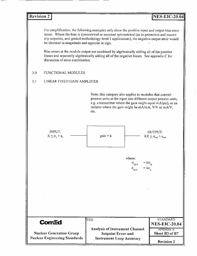
For simplification, the following examples only show the positive input and output bias error terms. Where the bias is symmetrical or assumed symmetrical (as in protection and reactor trip setpoints, and graded methodology level 1 applications), the negative output error would be identical in magnitude and opposite in sign.
Bias errors at the module output are combined by algebraically adding all of the positive biases and separately algebraically adding all of the negative biases. See appendix C for discussion of error combination.
3.0 FUNCTIONAL MODULES
3.1 LINEAR FIXED GAIN AMPLIFIER
Note: this category also applies to modules that convert process units at the input into different output process units, e.g. a transmitter where the gain might equal mA/psi), or an isolator where the gain might be mA/mA, V/V or mA/V, etc.
INPUT: X + C. +e\
OUTPUT: kX + Oou, + eout
where: a = ka
OUT X e = ke OUT X
Title STANDARD
CornEd NES-EIC-20.04 Analysis of Instrument Channel APPENDIX B
Nuclear Generation Group Setpoint Error and Sheet B3 of B7 Nuclear Engineering Standards Instrument Loop Accuracy
Revision 2
gain = k

INES-EIC-20.04
3.2 SUMMING AMPLIFIER
X:gain = k1
Y gain = k2
OUTPUT: (kI *X) + (k2 * Y) ± FOUT +eOUT
where:
CYOUT = [(kl*Uy) +(k2* ]
eOUT = (kl*ex) + (k2 * e Y)
3.3 MULTIPLIER
X gain= kl
Y gain = k2
I *X) OUTPUT: (k I *X) * (k2 * Y) ± FOUT +eOUT
where:2 2 1/2
CYOUT • (kI *k2)[(X*-y ) + (Y*Gx)
e OUT (k] *k2)[(X*e y) + (Y*ex)]
CYOUT is an approximation since it is assumed that the
individual input errors are small and their cross product is negligible. See reference 3.2 for the complete equation.
Latest Revision indicated by a bar in right hand margin. -
Title STANDARD CbmEd NES-EIC-20.04
Analysis of Instrument Channel APPENDIX B Nuclear Generation Group Setpoint Error and Sheet B4 of B7
Nuclear Engineering Standards Instrument Loop Accuracy Revision 2
X INPUT: X ± Fx +ex
Y INPUT: Y ± Fy +ey
X INPUT: X ± Fx +ex
Y INPUT: Y ± Fy +ey

INES-EIC-20.04Revision 2D
.3.4 DIVIDER
X INPUT: X ± Fx +ex
Y INPUT: Y ± Fy +ey
Xgain = kl
Y gain = k2
OUTPUT: "(kI *X)/(k2 * Y) ± FOUT +eOUT
where:
ki (( X(7 ) + (X Xcy)2 )1/2 1 eOUT kg_(Y ]
eorr k-(Yxex)-(Xxey).
3.5 MULTIPLIER DIVIDER
X INPUT: X ± Fx +ex
Y INPUT: Y ± Fy +ev
Z INPUT: Z ± Fz +ez
module gain = k OUTPUT: (k *)X * Y)/Z - Fo +eoUT
A
where:
C oU T kk iix oj) + x ar + - -x (3Z j) 2
e01/. z:k x ex +Lx
zx ey Y ez2]
Title STANDARD Cofld NES-EIC-20.04
Analysis of Instrument Channel APPENDIX B Nuclear Generation Group Setpoint Error and Sheet B5 of B7
Nuclear Engineering Standards Instrument Loop Accuracy Revision 2 L _________________________________Revision ____2
INES-EIC-20.04Revision 2
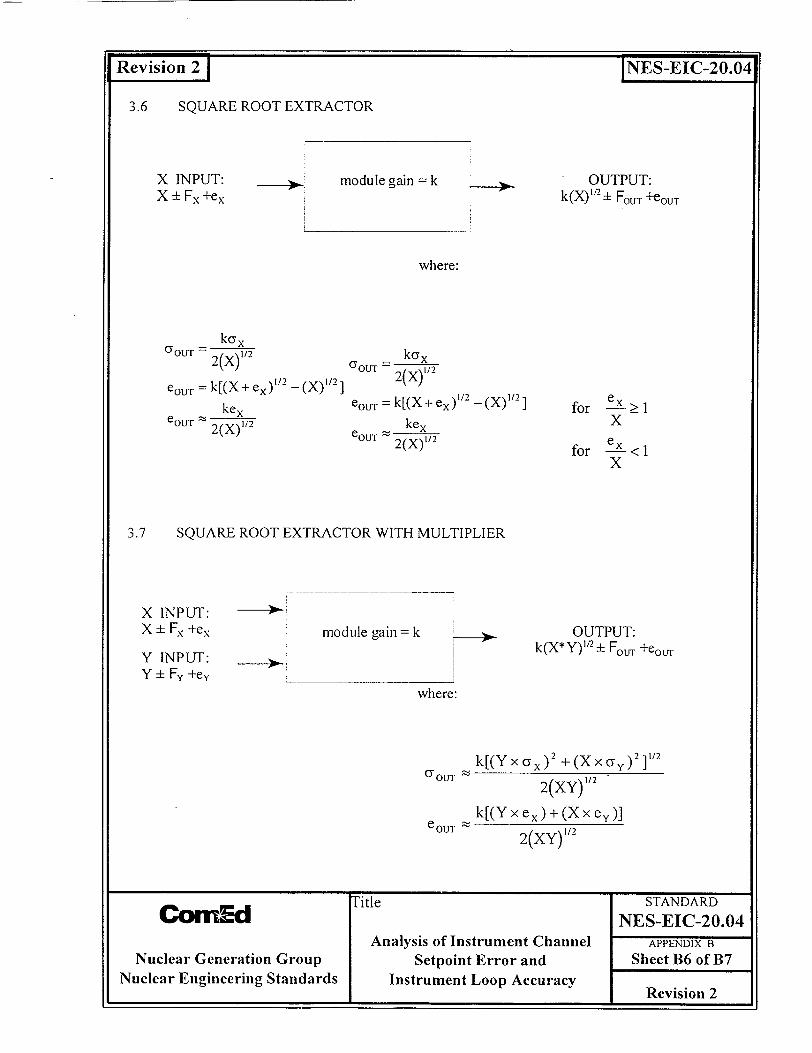
3.6 SQUARE ROOT EXTRACTOR
module gain = k OUTPUT: k(X) 1-"± FOUT +eOUT
where:
kaX CFOUT -- 2(X)12
eouT = k[(X + ex)1/2 _ (X)ll2 ]
eOUT 1 kex 2(X)11
0 0U - kcyx
2(X)1/2
eouT= k[(X + ex) 1 2 _ (X)" 1]
kex 2(X)" 2
for --X>l x for ex <1
x
3.7 SQUARE ROOT EXTRACTOR WITH MULTIPLIER
module gain = k OUTPUT: k(X*Y) 4- ± FOUT +eo0 Tr
where:
GY OUT lk[(Y x oYX) 2 +(Xx Cry) 2]V2
k[(Y x ex) + (X x ey)] eouT 2(XY) 1/
Title STANDARD COrnEd NES-EIC-20.04
Analysis of Instrument Channel APPENDIX B
Nuclear Generation Group Setpoint Error and Sheet B6 of B7 Nuclear Engineering Standards Instrument Loop Accuracy
I b.-1 F Revision 2
X INPUT: X - Fx +ex
X INPUT: X ± Fx +ex
Y INPUT: Y ± Fy +ey
2(XY) 1/2
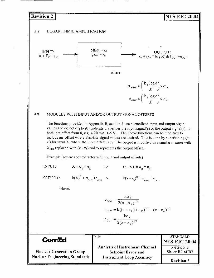
IRevision2L INES-EIC-20.04
3.8 LOGARITHMIC AMPLIFICATION
INPUT: X ± Fx+ ex
offset = k, gain k2
OUTPUT: "ki + (k2 * log X) ± FoT +eo0 T
where:
e0 OU (k 2 loge a k=2 log e_
e5OUT, _X_) ( xe
4.0 MODULES WITH INPUT AND/OR OUTPUT SIGNAL OFFSETS
The functions provided in Appendix B, section 3 use normalized input and output signal values and do not explicitly indicate that either the input signal(s) or the output signal(s), or both, are offset from 0, e.g. 4-20 mA, 1-5 V. The above functions can be modified to include an offset where absolute signal values are desired. This is done by substituting (x x,) for input X where the input offset is x,. The output is modified in a similar manner with XOUT replaced with (x - xo) and x0 represents the output offset.
Example (square root extractor with input and output offsets)
X±-(a +e X X
k(X) OU T +e
(x- xl) -t(3 + e x x
k(x-x)•+±a +e O- OUT OUT
2(x - xo )1/2
eOUT = k((x-x 0 )+ex ) 2 -(x-x 0 )1 2
e 2(x - X.
Title STANDARD C•lnEd NES-EIC-20.04
Analysis of Instrument Channel APPENDIX B Nuclear Generation Group Setpoint Error and Sheet B7 of B7
Nuclear Engineering Standards Instrument Loop Accuracy Revision 2
INPUT:
OUTPUT:
where:

�onLJ I NES-EIC-20.04
APPENDIX C
EQUATIONS FOR INSTRUMENT CHANNEL UNCERTAINTIES,
SETPOINTS AND ALLOWABLE VALUES
Latest Revision indicated by a bar in right hand margin.
STANDARD Co nEd Analysis of Instrument Channel NES-EIC-20.04
Setpoint Error and APPENDIX C
Nuclear Operations Division Instrument Loop Accuracy Sheet C1 of C7 Nuclear Engineering Standards Revision 2
Revision 2 1 INES-EIC-20.04
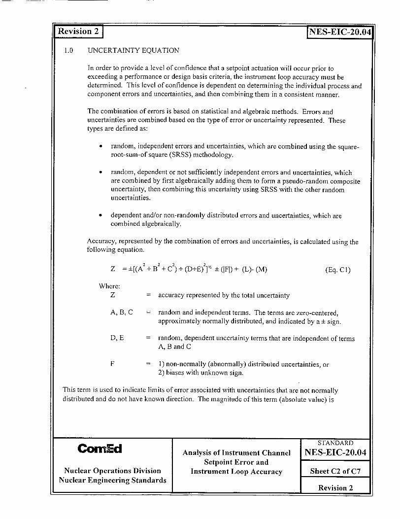
Revision 2 ] INES-EIC-20.04
1.0 UNCERTAINTY EQUATION
In order to provide a level of confidence that a setpoint actuation will occur prior to exceeding a performance or design basis criteria, the instrument loop accuracy must be determined. This level of confidence is dependent on determining the individual process and component errors and uncertainties, and then combining them in a consistent manner.
The combination of errors is based on statistical and algebraic methods. Errors and uncertainties are combined based on the type of error or uncertainty represented. These types are defined as:
"* random, independent errors and uncertainties, which are combined using the squareroot-sum-of square (SRSS) methodology.
" random, dependent or not sufficiently independent errors and uncertainties, which are combined by first algebraically adding them to form a pseudo-random composite uncertainty, then combining this uncertainty using SRSS with the other random uncertainties.
"* dependent and/or non-randomly distributed errors and uncertainties, which are combined algebraically.
Accuracy, represented by the combination of errors and uncertainties, is calculated using the following equation.
Z = ±[(A + B + C) + (D+E) '] + (IFI) + (L)- (M) (Eq. Cl)
Where: Z = accuracy represented by the total uncertainty
A, B, C = random and independent terms. The terms are zero-centered, approximately normally distributed, and indicated by a ± sign.
D, E = random, dependent uncertainty terms that are independent of terms A, B and C
F = 1) non-normally (abnormally) distributed uncertainties, or 2) biases with unknown sign.
This term is used to indicate limits of error associated with uncertainties that are not normally distributed and do not have known direction. The magnitude of this term (absolute value) is
STANDARD Co• Ed Analysis of Instrument Channel NES-EIC-20.04
Setpoint Error and Nuclear Operations Division Instrument Loop Accuracy Sheet C2 of C7
Nuclear Engineering Standards I I_ Revision 2
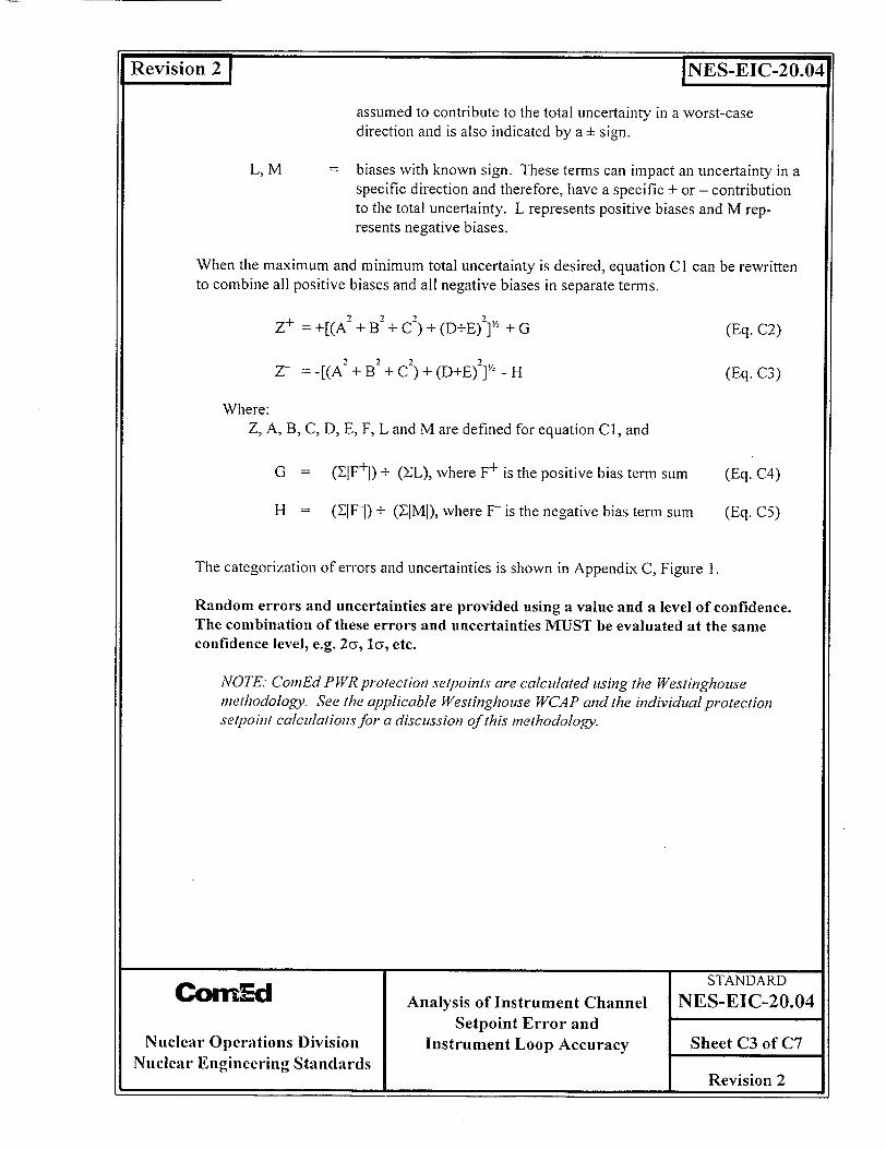
Revision 2 1
L, M
INES-EIC-20.04
assumed to contribute to the total uncertainty in a worst-case direction and is also indicated by a ± sign.
biases with known sign. These terms can impact an uncertainty in a specific direction and therefore, have a specific + or - contribution to the total uncertainty. L represents positive biases and M represents negative biases.
When the maximum and minimum total uncertainty is desired, equation Cl can be rewritten to combine all positive biases and all negative biases in separate terms.
Z+ +[(A-2 + B2 + C) + (D+E) + G
Z- = -[(A + B + C-) + (D+E)] - H
(Eq. C2)
(Eq. C3)
Where: Z, A, B, C, D, E, F, L and M are defined for equation Cl, and
G = (XIF+I) + (EL), where F+ is the positive bias term sum
H = (IF-I) + (-IMI), where F- is the negative bias term sum
(Eq. C4)
(Eq. C5)
The categorization of errors and uncertainties is shown in Appendix C, Figure 1.
Random errors and uncertainties are provided using a value and a level of confidence. The combination of these errors and uncertainties MUST be evaluated at the same confidence level, e.g. 2u, la, etc.
NOTE: CornEd PWR protection setpoints are calculated using the Westinghouse methodology. See the applicable Westinghouse WCAP and the individual protection setpoin! calculations for a discussion of this methodology.
STANDARD CObm d Analysis of Instrument Channel NES-EIC-20.04
Setpoint Error and Nuclear Operations Division Instrument Loop Accuracy Sheet C3 of C7
Nuclear Engineering Standards I_ I_ F Revision 2
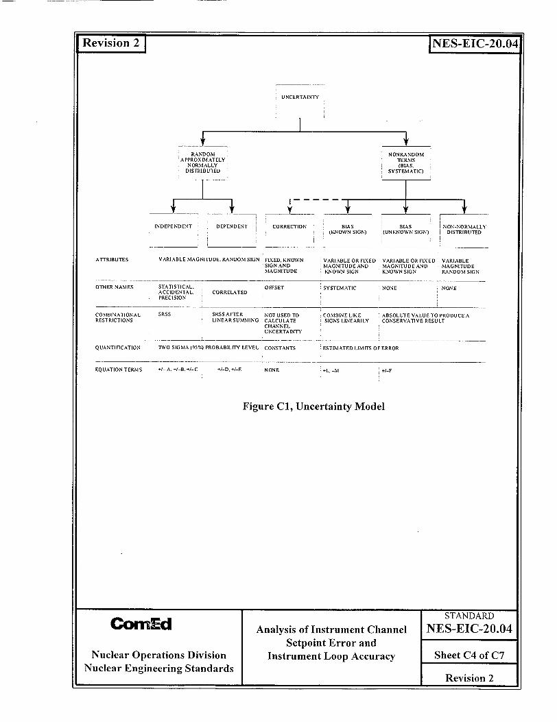
INES-EIC-20.04
UNCERTAINTY
NONPRANDO M TERMS (BIAS.
SYSTEMATIC)
I + ___
INDEPENDENT DEPENDENT CORRECTION BIAS BIAS
(KNOWN SIGN) (UNKNOWN SIGN)NON-NORMALLY
DISTRIBUTED
ATTRIBUTES VARIABLE MAGNITUDE. RANDOM
OTHER NAMES STATISTICAL. ACCIDENTAL. PRECISION
CORRELATED
SIGN FIXEDKNOWN VARIABLE OR FLXED SIGN AND MAGNITUDE AND MAGNITUDE KNOWN SIGN
,OFFSET SYSTEMATIC
VARIABLE OR FIXED, VARIABLE MAGNITUDE AND MAGNITUDE KNOWN SIGN RANDOM SIGN
NONE NONE
SRSSAFTER NOT USED TO COMBINE LIKE LINEAR SUMMING CALCULATE SIGNS LINEARILY
CHANNEL UNCERTAINTY
ABSOLUTE VALUE TO PRODUCE A CONSERVATIVE RESULT
QUANTIFICATION TWO SIGMA (95%) PROBABILITY LEVEL CONSTANTS ý ESTIMATED LIMITS OF ERROR
NONE +L. -I +/-F
Figure C1, Uncertainty Model
STANDARD Co• Ed Analysis of Instrument Channel NES-EIC-20.04 Setpoint Error and
Nuclear Operations Division Instrument Loop Accuracy Sheet C4 of C7 Nuclear Engineering Standards
Revision 2
RANDOM APPROXIMATELY'
NORMALLY DISTRIBUTED
COMBINATIONAL RESTRICTIONS
SRSS
EQUATION TERM S

Revision 2 1
2.0 UNCERTAINTY EQUATIONS USING COMED SYMBOLOGY
2.1 CALIBRATION ERROR
The equation for calibration error (CAL) is defined using CornEd symbology:
CAL = ±[(RAMTE + TEMTE) 2 + REMTE 2 + STD2]'2
where: RAMTE TEMTE REMTE STD
RASTD TESTD RESTD
= M&TE Reference Accuracy = M&TE Temperature Error = M&TE Reading Error = Calibration Standard Error and is determined from the following
equation:STD = ±[(RASTD + TESTD)2 + RESTD2]11 2
= Calibration Standard Reference Accuracy = Calibration Standard Temperature Error - Calibration Standard Reading Error
(Eq. C7)
Where both input M&TE and output M&TE are used in the calibration of a calibration block, Eq. C6 is rewritten as follows:
CAL = ±[(RAMTEIN + TEMTEIN) + REMTEIN + STDIN- + (RAMTEOUT +
TEMTEOUT) + REMTEOUT + STDOUT2] 1/) (Eq. C8)
2.2 TOTAL ERROR
The symbols shown in Appendix A, Table I can be substituted into equation C I using the applicable default error classifications. Use of this equation should be consistent with the error classifications specific to each instrument loop. For example, if the vendor supplied drift error has been determined to be a bias error, an eD term would be added to the bias errors and the (:D term would be removed.
2 2 2 2 2 2 _+[eE +PYA +D +CAL +ST +•N ]/+ePe~V
eT +eH + eR + eS + elR + MAR] (Eq. C9)
where: all random errors are at the same confidence level and, PE = Process Error RA = Reference Accuracy
STANDARD
GonE [ Analysis of Instrument Channel NES-EIC-20.04
Setpoint Error and Nuclear Operations Division Instrument Loop Accuracy Sheet C5 of C7
Nuclear Engineering Standards 1_____ __ 6Revision 2
INES-EIC-20.04
(Eq. C6)
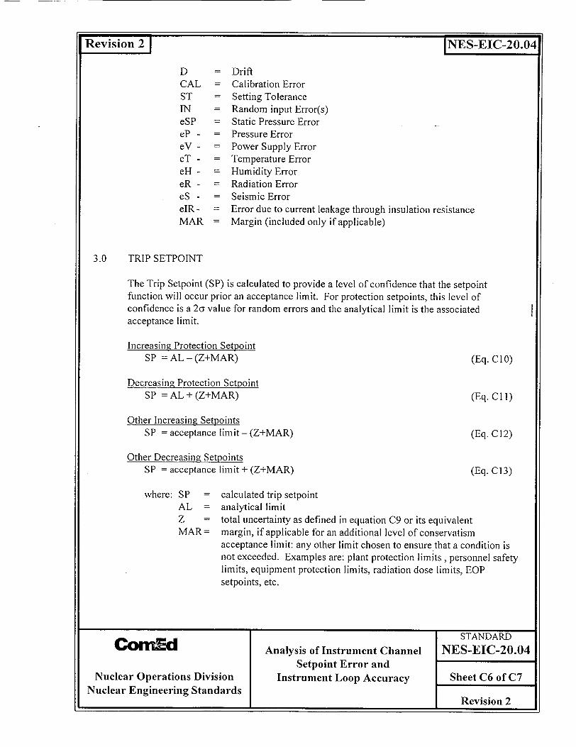
INES-EIC-20.04
D CAL ST IN eSP eP eV eT eHeReS eIR MAR
Drift Calibration Error Setting Tolerance Random input Error(s) Static Pressure Error Pressure Error Power Supply Error Temperature Error Humidity Error Radiation Error Seismic Error Error due to current leakage through insulation resistance Margin (included only if applicable)
3.0 TRIP SETPOINT
The Trip Setpoint (SP) is calculated to provide a level of confidence that the setpoint function will occur prior an acceptance limit. For protection setpoints, this level of confidence is a 2a value for random errors and the analytical limit is the associated acceptance limit.
Increasing Protection SetnointSP = AL - (Z+MAR)
Decreasing Protection Setpoint SP = AL + (Z+MAR)
Other Increasing Setpoints SP = acceptance limit - (Z+MAR)
Other Decreasin2 SetnointsSP = acceptance limit + (Z+MAR)
(Eq. C 10)
(Eq. C1 1)
(Eq. C 12)
(Eq. C13)
where: SP =
AL= z =
MAR=
calculated trip setpoint analytical limit total uncertainty as defined in equation C9 or its equivalent margin, if applicable for an additional level of conservatism acceptance limit: any other limit chosen to ensure that a condition is not exceeded. Examples are: plant protection limits, personnel safety limits, equipment protection limits, radiation dose limits, EOP setpoints, etc.
"STANDARD C[MLE[ Analysis of Instrument Channel NES-EIC-20.04
Setpoint Error and Nuclear Operations Division Instrument Loop Accuracy Sheet C6 of C7
Nuclear Engineering Standards I_ I_ I Revision 2
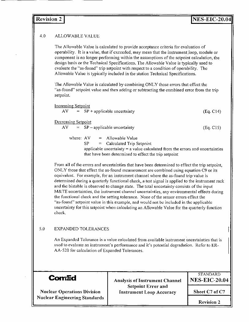
Revision 2 INES-EIC-20.04
4.0 ALLOWABLE VALUE
The Allowable Value is calculated to provide acceptance criteria for evaluation of operability. It is a value, that if exceeded, may mean that the instrument loop, module or component is no longer performing within the assumptions of the setpoint calculation, the design basis or the Technical Specifications. The Allowable Value is typically used to evaluate the "as-found" trip setpoint with respect to a condition of operability. The Allowable Value is typically included in the station Technical Specifications.
The Allowable Value is calculated by combining ONLY those errors that effect the "*as-found" setpoint value and then adding or subtracting the combined error from the trip setpoint.
Increasing Setpoint AV = SP + applicable uncertainty (Eq. C14)
Decreasing Setpoint AV = SP - applicable uncertainty (Eq. C15)
where: AV = Allowable Value
SP = Calculated Trip Setpoint applicable uncertainty = a value calculated from the errors and uncertainties that have been determined to effect the trip setpoint
From all of the errors and uncertainties that have been determined to effect the trip setpoint, ONLY those that effect the as-found measurement are combined using equation C9 or its equivalent. For example, for an instrument channel where the as-found trip value is determined during a quarterly functional check, a test signal is applied to the instrument rack and the bistable is observed to change state. The total uncertainty consists of the input M&TE uncertainties, the instrument channel uncertainties, any environmental effects during the functional check and the setting tolerance. None of the sensor errors effect the "as-found" setpoint value in this example, and would not be included in the applicable uncertainty for this setpoint when calculating an Allowable Value for the quarterly function check.
5.0 EXPANDED TOLERANCES
An Expanded Tolerance is a value calculated from available instrument uncertainties that is used to evaluate an instrument's performance and it's potential degradation. Refer to ERAA-520 for calculation of Expanded Tolerances.
STANDARD conEd Analysis of Instrument Channel NES-EIC-20.04
Sctpoint Error and Nuclear Operations Division Instrument Loop Accuracy Sheet C7 of C7
Nuclear Engineering Standards _ F__3_ b. I I Revision 2
Revision 2 1 INES-EIC-20.04
APPENDIX D
GRADED APPROACH TO DETERMINATION OF
INSTRUMENT CHANNEL ACCURACY
Latest Revision indicated by a bar in right hand margin.
Title STANDARD CorEd NES-EIC-20.04
Analysis of Instrument Channel APPENDIX D
Nuclear Generation Group Setpoint Error and Sheet D1 of D8 Nuclear Engineering Standards Instrument Loop Accuracy Revision 2
Revision 2 2 ]NES-EIC-20.04
1.0 INTRODUCTION
The CornEd setpoint methodology was developed and is defined by this standard to provide the basis, consistent with ANSI/ISA-S67.04-Part I, for the determination of instrument setpoints, allowable values and instrument loop accuracy. This ISA standard defines the requirements for establishing and maintaining setpoints for nuclear safety-related instrumentation. In addition, ISA-RP67.04-Part II provides guidance for implementing ANSI/ISA-S67.04 and imposes rigorous requirements for instrument uncertainty calculations and setpoint determination for safety-related instrument setpoints in nuclear power plants.
ISA-RP67.04-Part II recognizes that the historical focus of ANSI/ISA-S67.04 was the class of setpoints associated with the analytical limits as determined in the accident analysis. These setpoints have typically been interpreted as the reactor protection (RP) and emergency safety features (ESF) setpoints The RP and ESF setpoints are those critical to ensuring that the integrity of the multiple barriers to the release of fission products are maintained. The Recommended Practice also states that setpoints that are not part of the safety analysis and are not required to maintain the integrity of the fission product barriers may not require the same level of rigor or detail as described by the Recommended Practice. For these non-RP and non-ESF setpoints, a graduated or "graded" approach is appropriate for setpoints that:
"* provide anticipatory inputs to the RP or ESF functions, but are not credited in the accident analysis or,
"* support operation of, but not the initiation of, the ESF setpoints.
ISA draft Technical Report, ISA-dTR67.04.09, "Graded Approaches to Setpoint Determination", is being prepared to provide further guidance in establishing classification schemes for setpoints and recommending an approach to translate these classification schemes into a methodology for determination of instrument loop accuracies and setpoints. The technical report requires that a "graded methodology" provide a consistent hierarchy of both rigor and conservatism for classifying, determining and subsequently maintaining setpoints.
This appendix provides a classification scheme and the associated graded methodology for the determination of instrument loop accuracy at ComEd nuclear stations. The instrument loop accuracy may then be used to determine the associated instrument setpoints The CoinEd "graded methodology" is summarized in Table D1.
0itle STANDARD
Cbrn d NES-EIC-20.04 Analysis of Instrument Channel APPENDIX D
Nuclear Generation Group Setpoint Error and Sheet D2 of D8 Nuclear Engineering Standards Instrument Loop Accuracy F Revision 2

Revision 2 1 INES-EIC-20.042.0 CLASSIFICATION
The CornEd graded methodology classifies instrument setpoints into four levels. These correspond to a "level of confidence" that the setpoint will perform its function with respect to a limit or other limiting criteria. These levels range from Level 1, which provides the highest confidence, to Level 4, which may only document engineering judgment.
The following sections identify instrument channel functions and the minimum level of confidence used when determining instrument loop accuracy. Those individuals preparing and reviewing instrument loop accuracy calculations may choose to perform a particular instrument loop accuracy calculation using a higher level of confidence. This basis for this decision shall be fully documented in the instrument loop accuracy calculation.
It is not the intent of this standard to identify every instrument function encountered in a nuclear station. The following sections should provide sufficient guidance for selecting the appropriate level of confidence for those instrument functions not explicitly identified. Care should be taken to ensure that the function of the setpoint is clearly identified and that the instrument loop accuracy is determined consistent with the following levels.
2.1 LEVEL 1
This level is consistent with the definition of nuclear safety-related instrumentation in ANSI/ISA-S67.04-Part I. These instruments provide setpoints that:
1) Provide emergency reactor shutdown 2) Provide containment isolation 3) Provide reactor core cooling 4) Provide for containment or reactor heat removal 5) Prevent or mitigate a significant release of radioactive material to the environment or
is otherwise essential to provide reasonable assurance that a nuclear power plant can be operated without undue risk to the health and safety of the public
For ComEd nuclear stations, this specifically includes all reactor protection system (RPS), emergency safety features (ESF), emergency core cooling system (ECCS), primary containment isolation system (PCIS) and secondary containment (SCIS) setpoints.
Title STANDARD Owrco NES-EIC-20.04
Analysis of Instrument Channel APPENDIX D
Nuclear Generation Group Setpoint Error and Sheet D3 of D8 Nuclear Engineering Standards Instrument Loop Accuracy rn 6 1Revision 2

Revision 2 INES-EIC-20.042.2 LEVEL 2
This level will include those setpoints that:
1) Ensure compliance with Technical Specification but are not-level 1 setpoints. 2) Provide setpoints or limits associated with RG 1.97, category A variables. 3) Provide setpoints or limits associated with station emergency operating procedure
(EOP) requirements.
The RG 1.97 category A variables are included in Level 2 since they provide the primary information required to permit the control room operator to take specific manually controlled actions for which no automatic control is provided and that are required for safety systems to accomplish their safety functions for design basis accident events.
Level 2 instrument loops are typically associated with those setpoints that provide the station operator with specific action values or limits used to verify plant status. This includes instrument loops that provide an indication of acceptable performance for structures, systems and components in the Technical Specifications.
Setpoints or limits contained in station EOPs that are RG 1.97 category A variables, or setpoints that provide specific action values are included in Level 2. Other EOP setpoints may be either Level 2 or 3 depending on their function.
2.3 LEVEL 3
This level will include those setpoints that:
1) Provide setpoints or limits associated with RG 1.97, category B, C or D variables. 2) Provide setpoints or limits associated with other regulatory requirements or
operating commitments, e.g. OSHA, EPA, etc. 3) Provide setpoints or limits that are clearly associated with personnel safety or
equipment protection.
The RG 1.97, category B, C and D variables are associated with contingency actions and may be included in EOPs or other written procedures.
Classification of EOP setpoints as a Level 3 setpoint shall be approved by the station EOP coordinator or other individual designated by the station operations department.
Title STANDARD ConEd NES-EIC-20.04
Analysis of Instrument Channel APPENDIX D Nuclear Generation Group Setpoint Error and Sheet D4 of D8
Nuclear Engineering Standards Instrument Loop Accuracy Revision 2
Revision 2 I NES-EIC-20.04
2.4 LEVEL 4
This level will include those setpoints that:
1) Provide setpoints or limits not identified with the requirements in levels 1, 2 or 3 above.
2) Require documentation of engineering judgment, industry or station experience, or other methods have been used to set or identify an operating limit.
Level 4 shall provide documentation of all non-ComEd methodologies used to establish instrument loop accuracies or instrument setpoints.
3.0 DETERMINATION OF INSTRUMENT LOOP ACCURACY
3.1 LEVELS OF CONFIDENCE
The level of confidence associated with the calculation enforces a gradation in rigor and conservatism to the instrument loop accuracy evaluation. Level I, the highest level of conservatism, is typically associated with a 95% level of confidence that the setpoint will provide its intended function prior to limit or limiting condition. Levels 2, 3 and 4 provide decreasing levels of confidence by allowing various additions to the methodology used to calculate and combine errors and uncertainties. At Level 4, the instrument loop accuracy may not be associated with any clearly identified level of confidence other than experience.
The methodology associated with each level is shown in Table Dl.
3.2 LEVEL I
Calculation of instrument loop accuracy, instrument setpoints and allowable values in Level I shall use the equations in App. C. These equations use a 2Ty level of confidence and require that determination of instrument loop accuracy always err on the side of conservatism.
Level I setpoints are consistent with ISA S67.04, Part I and ISA RP67.04, Part II. in order to ensure that protective actions occur 95% of the time with a high degree of confidence before the analytical limits are reached.
3.3 LEVEL 2
Level 2 instrument loop accuracy is calculated using the equations in Appendix C with the following exceptions:
I) Random errors are evaluated at a I u level of confidence
""itle STANDARD C• =-d NES-EIC-20.04
Analysis of Instrument Channel APPENDIX D Nuclear Generation Group Setpoint Error and Sheet D5 of D8
Nuclear Engineering Standards Instrument Loop Accuracy tý t7 I F Revision 2
Iso~ NE S- I - 0
2) Bias errors may be combined using SRSS in accordance with Reference 3.11 3) Where it can be determined that a setpoint function is only evaluated in a single
direction, either increasing or decreasing, single side of interest confidence levels may be utilized (reference 3.2, section 8.1).
3.4 LEVEL 3
Level 3 instrument loop accuracy is calculated using the equations in Appendix C, the exceptions in Level 2 and the following additional exceptions:
1) Uncertainties applicable to the entire instrument channel are used wherever available, e.g. channel drift and channel temperature uncertainty vs. module/component drift and module/component temperature uncertainty.
2) Where all terms are expected to be approximately normally distributed and the number of terms is >_4, the sum is assumed to be approximately distributed. Therefore, all terms can be combined using SRSS.
3) For bistables, the RA term does not require inclusion of the hysteresis/linearity components. Only the RA uncertainty OR the ST uncertainty, whichever is larger shall be used
3.5 LEVEL 4
Level 4 instrument loop accuracy may be calculated using the equations in Appendix C and include the exceptions in Level 2 and 3. For calculations associated with Level 4 instrument loops, the basis for determining the instrument loop accuracy shall be documented.
Title STANDARD COrnEd NES-EIC-20.04 Analysis of Instrument Channel APPENDIX D
Nuclear Generation Group Setpoint Error and Sheet D6 of D8 Nuclear Engineering Standards Instrument Loop Accuracy Revision 2
Revision 2 INES-EIC-20.04

I -
Revision 2 1 INES-EIC-20.04
Table D1, Graded Methodology
LEVEL TYPICAL METHO- APPLICABLE APPLICATION DOLOGY UNCERTAINTY
METHODS 1 * Protection setpoints 2a + Xei 0 Consistent with ISA S67.04, Part I
"* ESF/RPS/ECCS and ISA RP67.04, Part II. "* PCIS/SCIS
" Ensures protective actions occur 95% of the time with a high degree of confidence before the analytical limits are reached.
" Random and bias error combination:
Z = ±[A2 + B2 + C2 + (E +
F)21½ý ± (IFI) + (L) - (M)
Z resultant uncertainty, combination of random and bias uncertainties
A,B,C random, independent terms
D,E - random dependent terms (independent of A,B and C)
F = abnormally distributed uncertainties and/or bias (unknown sign)
L,M = biases with known sign 2 0 EOP operator action setpoints a + Zei 0 Bias errors combined using SRSS in
* RG 1.97 Type A variables accordance with ASME PTC 19.1:
ei = ±[F2 + L2 + M2 ]!/ where F, L and M are bias errors as shown above
Single side of interest confidence interval evaluation where the evaluated setpoint is in a single direction:
Z = 0.468& + Zei
Title STANDARD ComEd NES-EIC-20.04
Analysis of Instrument Channel APPENDIX D
Nuclear Generation Group Setpoint Error and Sheet D7 of D8 Nuclear Engineering Standards Instrument Loop Accuracy Revision 2
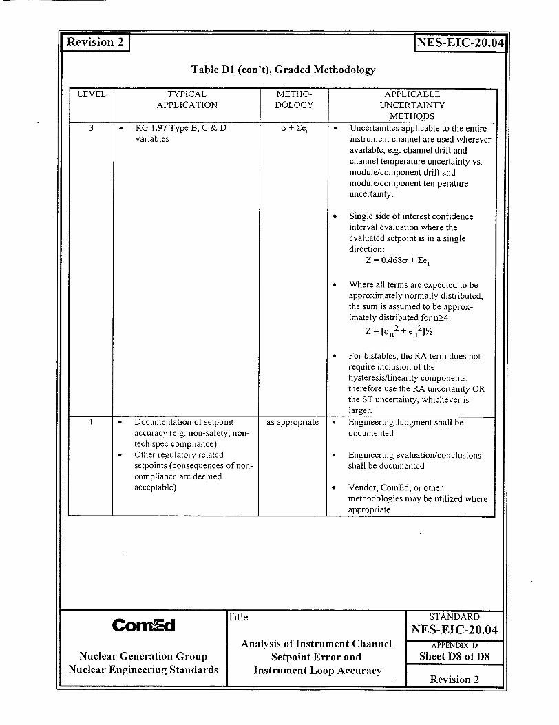
Revision 2 INES-EIC-20.04
Table D1 (con't), Graded Methodology
LEVEL TYPICAL METHO- APPLICABLE APPLICATION DOLOGY UNCERTAINTY
METHODS 3 * RG 1.97 Type B, C & D or + Iei Uncertainties applicable to the entire
variables instrument channel are used wherever available, e.g. channel drift and channel temperature uncertainty vs. module/component drift and module/component temperature uncertainty.
" Single side of interest confidence interval evaluation where the evaluated setpoint is in a single direction:
Z = 0.468cy + Eei
" Where all terms are expected to be approximately normally distributed, the sum is assumed to be approximately distributed for n>4:
Z = [n 2 +en 2 ]½A
"* For bistables, the RA term does not require inclusion of the hysteresis/linearity components, therefore use the RA uncertainty OR the ST uncertainty, whichever is larger.
4 * Documentation of setpoint as appropriate * Engineering Judgment shall be accuracy (e.g. non-safety, non- documented tech spec compliance)
* Other regulatory related 0 Engineering evaluation/conclusions setpoints (consequences of non- shall be documented compliance are deemed acceptable) • Vendor, CoinEd, or other
methodologies may be utilized where appropriate
T'itle STANDARD CbrnEd NES-EIC-20.04
Analysis of Instrument Channel APPENDIX D
Nuclear Generation Group Setpoint Error and Sheet D8 of D8 Nuclear Engineering Standards Instrument Loop Accuracy
I I . F Revision 2 J

I -
IRevision 2 INES-EIC-20.04
APPENDIX E
REACTOR WATER LEVEL TO SENSOR dP CONVERSION
.Latcst Revision indicated by a bar in right hand margin. .,
Title STANDARD CbmEd NES-EIC-20.04 Analysis of Instrument Channel APPENDIX E
Nuclear Generation Group Setpoint Error and Sheet El of E8 Nuclear Engineering Standards Instrument Loop Accuracy
I t") 0 1 F Revision 2
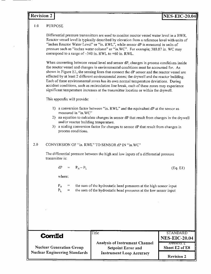
Zevision 2 1 INES-EIC-20.04
1.0 PURPOSE
Differential pressure transmitters are used to monitor reactor vessel water level in a BWR. Reactor vessel level is typically described by elevation from a reference level with units of "inches Reactor Water Level" or "in. RWL", while sensor dP is measured in units of pressure such as "inches water column" or "in.WC". For example; 380.87 in. WC may correspond to a range of -340 in. RWL to +60 in. RWL.
When converting between vessel level and sensor dP, changes in process conditions inside the reactor vessel and changes in environmental conditions must be accounted for. As shown in Figure El, the sensing lines that connect the dP sensor and the reactor vessel are effected by at least 2 different environmental zones; the drywell and the reactor building. Each of these environmental zones has its own normal temperature deviations. During accident conditions, such as recirculation line break, each of these zones may experience significant temperature increases at the transmitter location or within the drywell.
This appendix will provide:
1) a conversion factor between "in. RWL" and the equivalent dP at the sensor as measured in "in.WC"
2) an equation to calculate changes in sensor dP that result from changes in the drywell and/or reactor building temperature.
3) a scaling conversion factor for changes to sensor dP that result from changes in process conditions.
2.0 CONVERSION OF "in. RWL" TO SENSOR dP IN "in.WC"
The differential pressure between the high and low inputs of a differential pressure transmitter is:
dP PH - PL (Eq. El)
where:
PH = the sum of the hydrostatic head pressures at the high sensor input PL = the sum of the hydrostatic head pressures at the low sensor input
f'itle STANDARD Cornf : NES-EIC-20.04
Analysis of Instrument Channel APPENDIX E Nuclear Generation Group Setpoint Error and Sheet E2 of E8
Nuclear Engineering Standards Instrument Loop Accuracy Revision 2
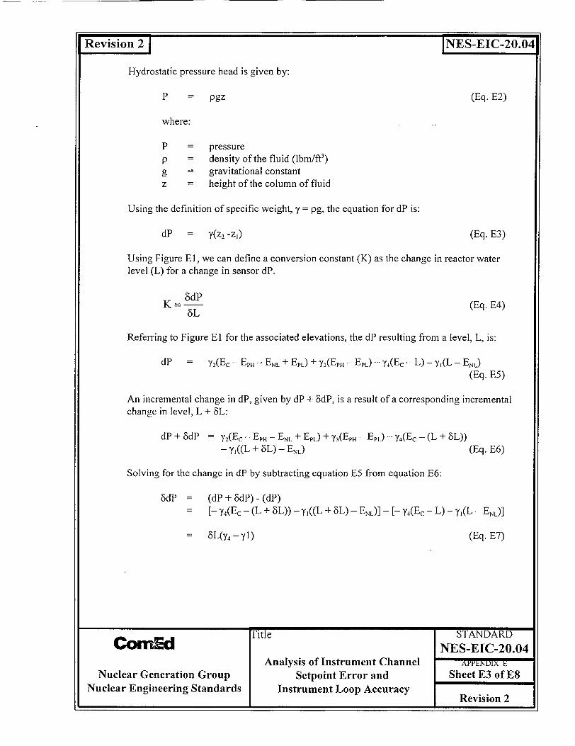
Revision 2 1
Hydrostatic pressure head is given by:
P = pgz
where:
P
p g z
pressure density of the fluid (Ibm/ft) gravitational constant height of the column of fluid
Using the definition of specific weight, y = pg, the equation for dP is:
dP = y(z, -zj)
Using Figure El, we can define a conversion constant (K) as the change in reactor water level (L) for a change in sensor dP.
K 8dP 8L (Eq. E4)
Referring to Figure El for the associated elevations, the dP resulting from a level, L, is:
dP = y2(Ec - EPH - ENL + EPL) + 7 3(EPH - EPL) - y4(Ec - L) - yi(L - ENL)
(Eq. E5)
An incremental change in dP, given by dP + WdP, is a result of a corresponding incremental change in level, L + KL:
dP + 5dP = y2(Ec - EPH - ENL + EPL) + y3(EPH - EPL) - y4(Ec - (L + 8L)) - y.((L + 5L) - ENL) (Eq. E6)
Solving for the change in dP by subtracting equation E5 from equation E6:
6dP = (dP + 5dP) - (dP) P Y4(Ec - (L + 8L)) - y1((L + 6L) - ENL)] - [- y4(Ec - L) - yi(L - ENL)]
6L(y 4 - Y1) (Eq. E7)
Title STANDARD CornEd NES-EIC-20.04
Analysis of Instrument Channel APPENDIX E
Nuclear Generation Group Setpoint Error and Sheet E3 of E8 Nuclear Engineering Standards Instrument Loop Accuracy Revision 2
INES-EIC-20.04
(Eq. E2)
(Eq. E3)
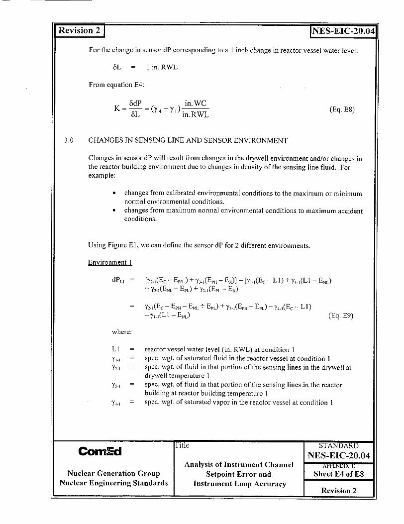
Revision 2 1 INES-EIC-20.04
For the change in sensor dP corresponding to a 1 inch change in reactor vessel water level:
61, = I in. RWL
From equation E4:
6dP in.WC K = 8L = (Y4 -YI) in. RWL (Eq. E8)
3.0 CHANGES IN SENSING LINE AND SENSOR ENVIRONMENT
Changes in sensor dP will result from changes in the drywell environment and/or changes in the reactor building environment due to changes in density of the sensing line fluid. For example:
"• changes from calibrated environmental conditions to the maximum or minimum normal environmental conditions.
"* changes from maximum normal environmental conditions to maximum accident conditions.
Using Figure El, we can define the sensor dP for 2 different environments.
Environment 1
dPL= [72- 1(Ec - EpH ) + y3-1(EpH - Ex)] - [y1,.(Ec - LI) + y4.1(LI - ENL)
+ Y2.1(ENL - EPL) + 73.](EPL - Ex)
y72-1(Ec - EPH - ENL + EPL) + Y3- 1(EpH - EPL) - 74.I(Ec - L ) - y1.1 (L - ENL) (Eq. E9)
where:
LI reactor vessel water level (in. RWL) at condition 1 TI-1 = spec. wgt. of saturated fluid in the reactor vessel at condition I y2.• = spec. wgt. of fluid in that portion of the sensing lines in the drywell at
drywell temperature I 3-1= spec. wgt. of fluid in that portion of the sensing lines in the reactor
building at reactor building temperature I "Y4.1 = spec. wgt. of saturated vapor in the reactor vessel at condition 1
"f'itle STANDARD COM 4Ed NES-EIC-20.04
Analysis of Instrument Channel APPENDIX E
Nuclear Generation Group Setpoint Error and Sheet E4 of E8 Nuclear Engineering Standards Instrument Loop Accuracy Revision 2

I --
Revision32
Environment 2
dPL2 = y2-2(Ec - EPH - ENL + EPL) + Y3-2(EPH - EPL) - 7 4.2(Ec - L2) - 1.:2(L2 - ENL) (Eq. E 10)
where:
L2 "Y1-2
Y2-2
"Y3-2
Y4-2
= reactor vessel water level (in. RWL) at condition 2 = spec. wgt. of saturated fluid in the reactor vessel at condition 2
spec. wgt. of fluid in that portion of the sensing lines in the drywell at drywell temperature 2
= spec. wgt. of fluid in that portion of the sensing lines in the reactor building at reactor building temperature 2
= spec. wgt. of saturated vapor in the reactor vessel at condition 2
If we assume all changes between environment 1 and environment 2 are limited to changes in the drywell and reactor building environments:
LI
Y4-1
= L2 71 '/-2
= Y/4-2
The change in sensor dP from condition I to condition 2 is:
AdP = dPL2- dPLI
= [('/2-2 '/2- 1)(Ec - EPH - ENL + EPL)] + [(3-2 - Y/3-)(EPH - EPL)]
(Eq. El 1)
3.1 EXAMPLE
To calculate the process error due to a LOCA, we need to determine the change in sensor dP between maximumn normal environmental conditions and the maximum accident environmental conditions in the drywell and reactor building. This is typically calculated at a specific reactor vessel level, e.g. one of the vessel level protection setpoints. In addition, in order to calculate a bounding change, the following assumptions apply:
1) Transient effects are ignored. It is assumed that the sensing lines are at thermal equilibrium with their environment.
2) Reactor vessel process conditions do not change, only the sensing line environments are effected by the LOCA. Obviously the reactor vessel saturation conditions will change if a scram occurs, but in this example we are looking only for the process error at the protection level setpoint.
folEd Title STANDARD NES-EIC-20.04
Analysis of Instrument Channel APENIXx Nuclear Generation Group Setpoint Error and Sheet E5 of E8
Nuclear Engineering Standards Instrument Loop Accuracy I t- Revision 2
INES-EIC-20.04
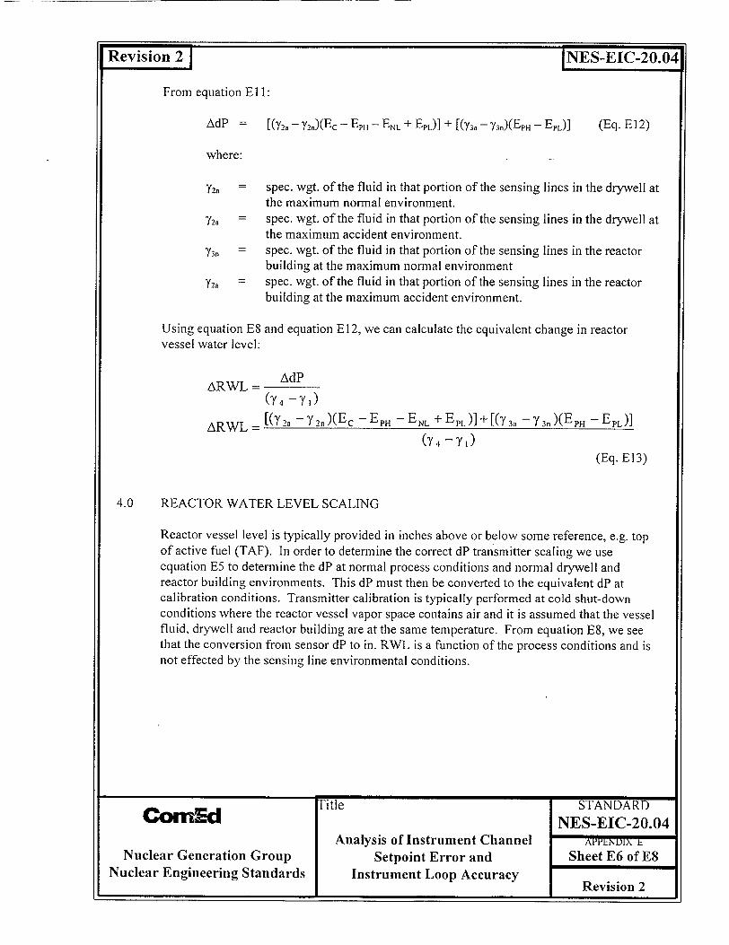
I -
Revision 2 INES-EIC-20.04
From equation E 11:
AdP = [(Y2. - Y2.)(Ec - EPH - ENL + EPL)] + [(Y3a - Y3f)(EPH - EPL)] (Eq. E12)
where:
Y2,, = spec. wgt. of the fluid in that portion of the sensing lines in the drywell at the maximum normal environment.
72a = spec. wgt. of the fluid in that portion of the sensing lines in the drywell at the maximum accident environment.
3n = spec. wgt. of the fluid in that portion of the sensing lines in the reactor building at the maximum normal environment
Y2_a = spec. wgt. of the fluid in that portion of the sensing lines in the reactor building at the maximum accident environment.
Using equation E8 and equation E12, we can calculate the equivalent change in reactor vessel water level:
ARWL = AdP (74 -Y.)
ARWL = (Y2a Y2n)(E c - E PH- ENL + E PL )] [( 3a -- Y 3n )(E PH - EPL)
(Y(E -71) (Eq. E 13)
4.0 REACTOR WATER LEVEL SCALING
Reactor vessel level is typically provided in inches above or below some reference, e.g. top of active fuel (TAF). In order to determine the correct dP transmitter scaling we use equation E5 to determine the dP at normal process conditions and normal drywell and reactor building environments. This dP must then be converted to the equivalent dP at calibration conditions. Transmitter calibration is typically performed at cold shut-down conditions where the reactor vessel vapor space contains air and it is assumed that the vessel fluid, drywell and reactor building are at the same temperature. From equation E8, we see that the conversion from sensor dP to in. RWL is a function of the process conditions and is not effected by the sensing line environmental conditions.
fitle STANDARD C€om~ d NES-EIC-20.04
Analysis of Instrument Channel APPENDIX E
Nuclear Generation Group Setpoint Error and Sheet E6 of E8 Nuclear Engineering Standards Instrument Loop Accuracy Revision 2
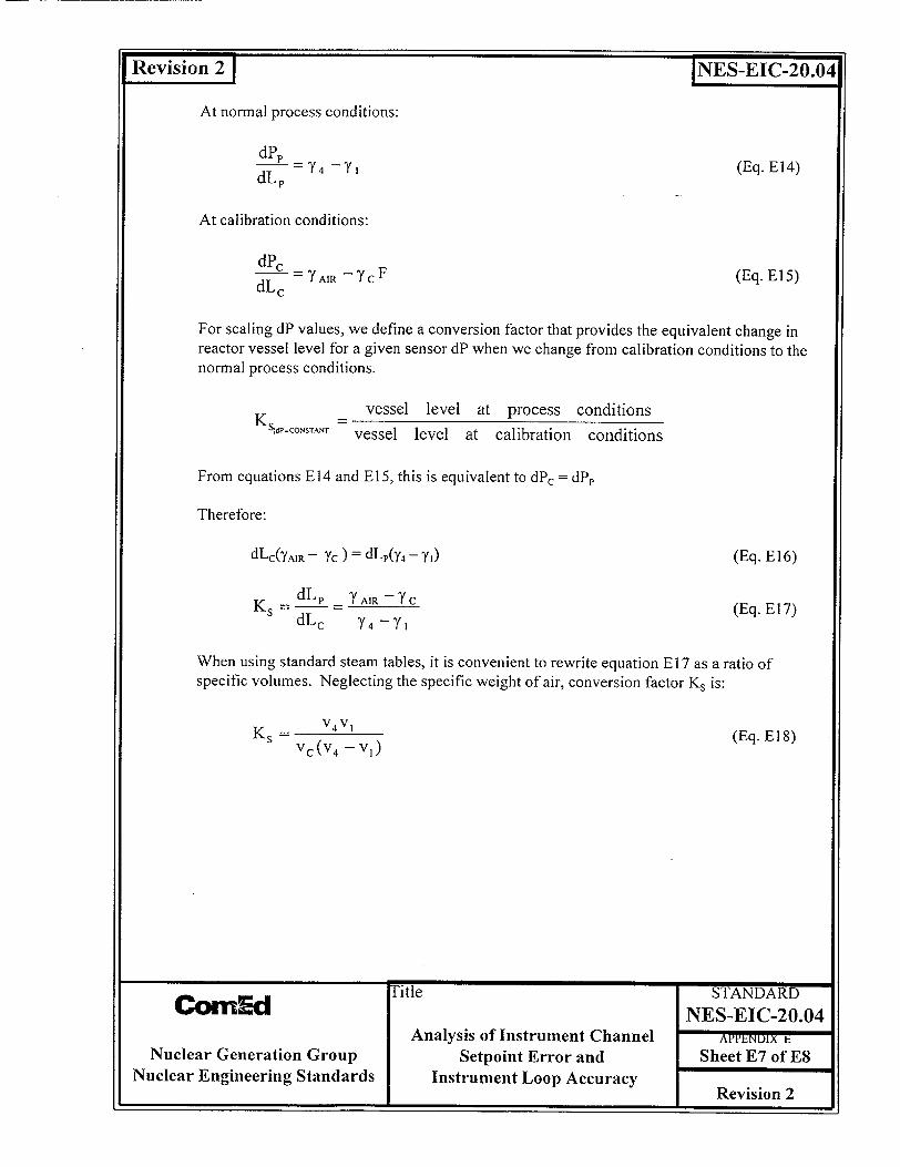
Revision 2 J
At normal process conditions:
dPp dL p
At calibration conditions:
dPc d-C YAIR-ycF dLc (Eq. E15)
For scaling dP values, we define a conversion factor that provides the equivalent change in reactor vessel level for a given sensor dP when we change from calibration conditions to the normal process conditions.
vesse~l level at nflprc!IK I. CONSTANT -F
.t JLA&141 vessel level at calibration conditions
From equations E14 and E15, this is equivalent to dPc = dP,
Therefore:
dLc(YAIR - 7c ) = dLp(y 4 -70
K dL p7 A --IRC dLc 74 -71
(Eq. E16)
(Eq. E17)
When using standard steam tables, it is convenient to rewrite equation E17 as a ratio of specific volumes. Neglecting the specific weight of air, conversion factor Ks is:
KS- v 4 v1 K C = (V 4 -VI) (Eq. E 18)
NTitle STANDARD Cbrn d NES-EIC-20.04
Analysis of Instrument Channel APPENDIX h
Nuclear Generation Group Setpoint Error and Sheet E7 of E8 Nuclear Engineering Standards Instrument Loop Accuracy Revision 2
INES-EIC-20.04
(Eq. E14)
Pnnr1;t;nnc
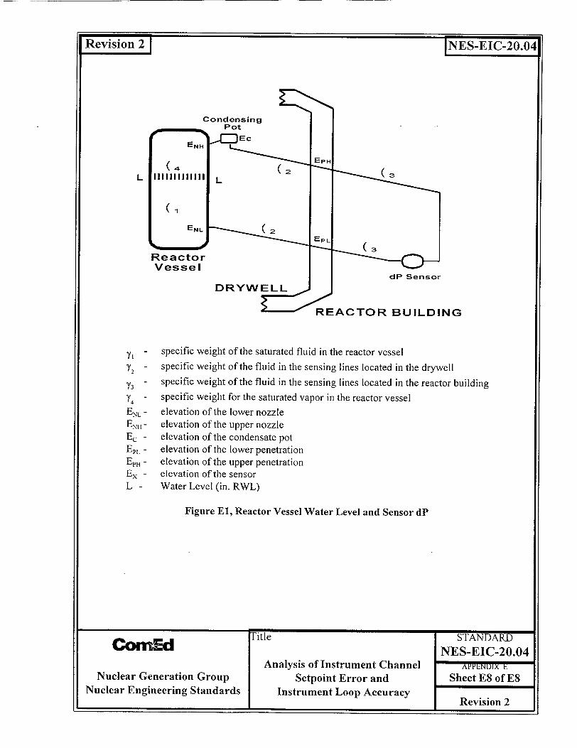
Revision2
L
'YI "/2
Y/3
ENL
ENH
Ec
EPL
EpH
Ex L -
INES-EIC-20.04
Condensing Pot
Ec ENH
1(4(23 L
teactor /essel
dP Sensor DRYWELL
'REACTOR BUILDING
specific weight of the saturated fluid in the reactor vessel specific weight of the fluid in the sensing lines located in the drywell specific weight of the fluid in the sensing lines located in the reactor building specific weight for the saturated vapor in the reactor vessel elevation of the lower nozzle elevation of the upper nozzle elevation of the condensate pot elevation of the lower penetration elevation of the upper penetration elevation of the sensor Water Level (in. RWL)
Figure El, Reactor Vessel Water Level and Sensor dP
"Mr-0 Title STANDARD commad NES-EIC-20.04
Analysis of Instrument Channel APPENDIXT Nuclear Generation Group Setpoint Error and Sheet E8 of E8
Nuclear Engineering Standards Instrument Loop Accuracy Revision 2
Revision 2 J [NES-EIC-20.04
APPENDIX F
TEMPERATURE EFFECTS ON LEVEL MEASUREMENT
SLatest Revision indicated by a bar in right hand margin.
Title STANDARD Cornld NES-EIC-20.04
Analysis of Instrument Channel APPENDIX F
Nuclear Generation Group Setpoint Error and Sheet F1 of F14 Nuclear Engineering Standards Instrument Loop Accuracy Revision 2

Revision 2 INES-EIC-20.04
1.0 INTRODUCTION
Differential pressure level measurement systems are typically calibrated for a specific set of operating conditions, i.e. processes pressure and reference leg temperature. If either of these conditions change, an error will be introduced between the actual level and the indicated level. This is due to changes in the dP at the sensor and results from changes in fluid density and not from changes in actual level. Since this error is of known magnitude and known direction (based on the difference between the calibrated condition and the new process and/or environmental condition), it is treated as a bias error.
This appendix provides simplified formulas for estimating the effects of:
"* process pressure changes (assuming that the vessel is at saturation conditions), "* environmental changes (assuming that the reference leg fluid temperature is at
equilibrium with the environment), and "* both process changes and reference leg temperature changes acting simultaneously
to produce a worst case bias under specified conditions.
2.0 ERROR FRACTION
When evaluating the effects of process and environmental changes on level measurement accuracy, it is convenient to consider these effects as changes from the known (or calibrated) condition. Using this concept, the level error is a function of how much the indicated level differs from the actual level. The indicated level (IND LVL) corresponds to the transmitter scaling relationship where transmitter output is a function of the dP applied to the transmitter. The scaling relationship should be based on specific process conditions and specific environmental conditions. The actual level (ACT LVL) will then deviate from the indicated level (IND LVL) as a function of the deviation of the process and environmental conditions from the calibrated conditions. This difference between indicated level and actual
level is defined as the "error fraction" (E)l:
E=% IND LVL-% ACTLVL
This appendix will use units of% level which is consistent with typical level measurement scales where indicated level ranges from 0% to 100% level. While units of level, and consequently E could be in other units, the derivations are simplified if % level is chosen.
The term "error fraction" and the equation E = % IND LVL - % ACT LVL, is consistent with the steam generator level protection and EOP setpoint accuracy evaluation originally provided by Westinghouse and currently incorporated in ComEd setpoint accuracy calculations for Byron and Braidwood stations.
Title STANDARD COMEc NES-EIC-20.04
Analysis of Instrument Channel APPENDIX F
Nuclear Generation Group Setpoint Error and Sheet F2 of F14 Nuclear Engineering Standards Instrument Loop Accuracy Revision 2
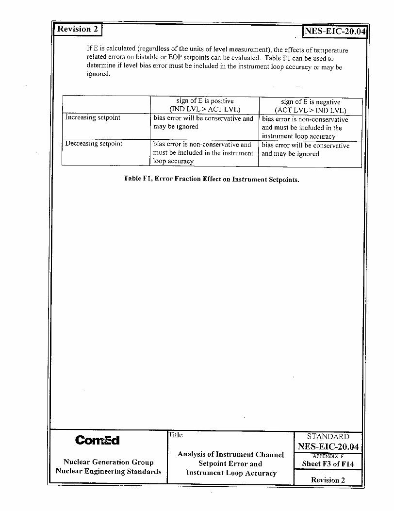
,n 2 INES-EIC-20.04
If E is calculated (regardless of the units of level measurement), the effects of temperature related errors on bistable or EOP setpoints can be evaluated. Table F1 can be used to determine if level bias error must be included in the instrument loop accuracy or may be ignored.
Table F1, Error Fraction Effect on Instrument Setpoints.
M" -Title STANDARD COM M NES-EIC-20.04 Analysis of Instrument Channel APPENDIX F
Nuclear Generation Group Setpoint Error and Sheet F3 of F14 Nuclear Engineering Standards Instrument Loop Accuracy
__________________________ Revision 2
sign of E is positive sign of E is negative (IND LVL > ACT LVL) (ACT LVL > IND LVL)
Increasing setpoint bias error will be conservative and bias error is non-conservative may be ignored and must be included in the
instrument loop accuracy Decreasing setpoint bias error is non-conservative and bias error will be conservative
must be included in the instrument and may be ignored loop accuracy
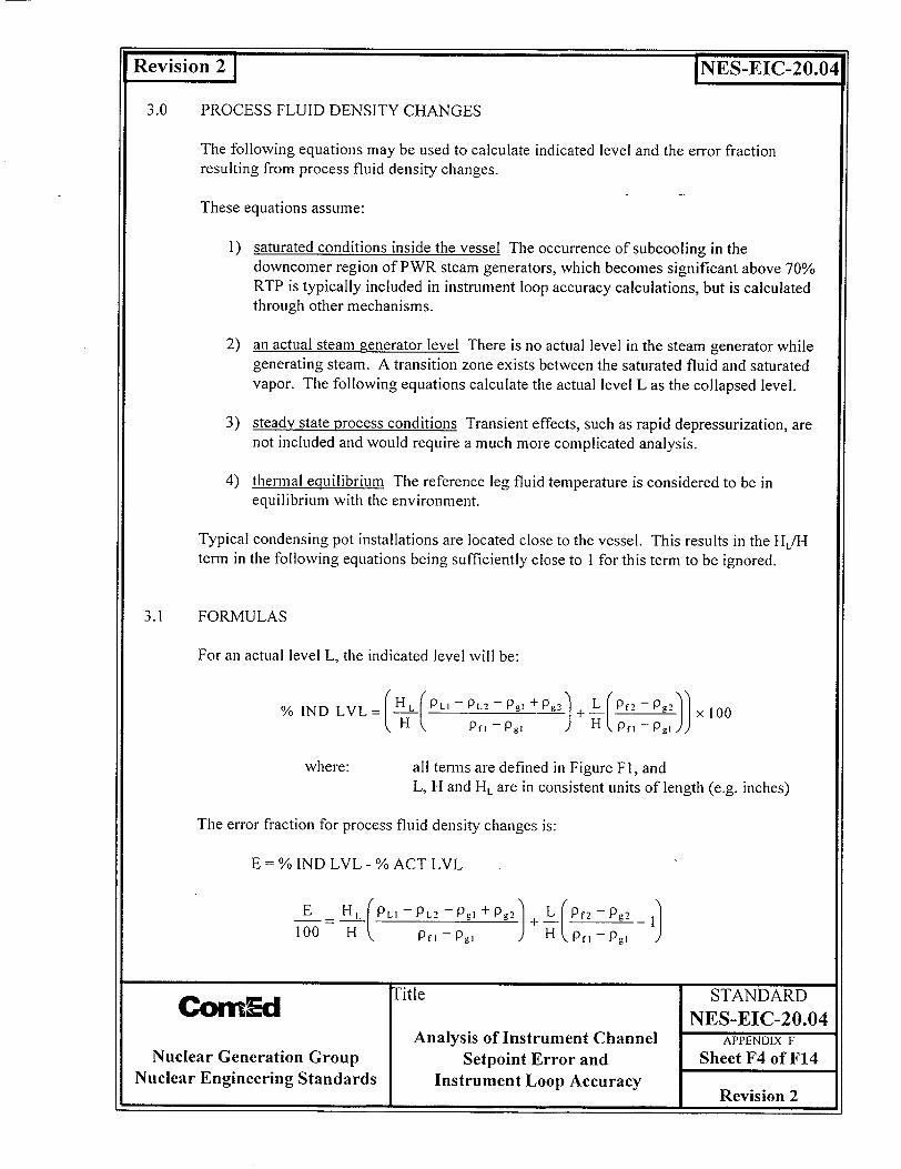
Revision 2 1 INES-EIC-20.04
3.0 PROCESS FLUID DENSITY CHANGES
The following equations may be used to calculate indicated level and the error fraction resulting from process fluid density changes.
These equations assume:
1) saturated conditions inside the vessel The occurrence of subcooling in the downcomer region of PWR steam generators, which becomes significant above 70% RTP is typically included in instrument loop accuracy calculations, but is calculated through other mechanisms.
2) an actual steam generator level There is no actual level in the steam generator while generating steam. A transition zone exists between the saturated fluid and saturated vapor. The following equations calculate the actual level L as the collapsed level.
3) steady state process conditions Transient effects, such as rapid depressurization, are not included and would require a much more complicated analysis.
4) thermal equilibrium The reference leg fluid temperature is considered to be in equilibrium with the environment.
Typical condensing pot installations are located close to the vessel. This results in the HL/H term in the following equations being sufficiently close to 1 for this term to be ignored.
3.1 FORMULAS
For an actual level L, the indicated level will be:
% IND LVL=- - pLI -- PL2--Pg + . ) +L( Pf2-Pg2 x 100 Pf] - P ,) H . Pfl- Ps j)
where: all terms are defined in Figure Fl, and L, H and HL are in consistent units of length (e.g. inches)
The error fraction for process fluid density changes is:
E=% IND LVL-%ACTLVL
E H LPLI - PL2-Pg+ Pg 2 + pf Pg2 100 H~ ( fP Pf I - P,]' - f gi
on -BdTitle STANDARD Corn~d NES-EIC-20.04
Analysis of Instrument Channel APPENDIX F
Nuclear Generation Group Setpoint Error and Sheet F4 of F14 Nuclear Engineering Standards Instrument Loop Accuracy FRevision 2

Revision 2 1Fluid
Fluid Level IIIII
Vessel
INES-EIC-20.04
H L /i H
dP Transmitter
L -distance from lower tap to fluid level
H - distance from lower tap to upper tap
H - distance from lower tap to center line of condesnsing pot
D, - fluid density
D - vapor density
D - reference leg fluid density
Pfl' P8I T, P
0 f '-- P gI
T REF LEG
PLI
PL2
- temperature and pressure inside the vessel at calibrated conditions - density of saturated liquid and steam at calibration conditions T and P - temperature and pressure inside the vessel at some new condition - density of saturated liquid and steam at the new conditions T and P 2 2
- temperature of the environment and reference leg fluid - density of reference leg liquid at TREFLEG and Pi (compressed liquid) - density of reference leg liquid at TF E and P_ (compressed liquid)
Figure FI: Level Bias Error Due to Process Fluid Density Changes
3.2 DERIVATION
Calculate the transmitter 0% and 100% level for the dP at T1 and P1 conditions:
= pgH -- (p gH + p g(HL - H))
= gH (PL - g)- gH(pn- Pgl) = PLIg Pg HL
dP H g -P gH 0%P/ I LI L g- L
= gHL(PL p5 1 )
Calculate the transmitter dP at L% level for the dP at T2 and P2 conditions:
L% = (L/H)x100% lvI
CoM][ Title STANDARD NES-EIC-20.04
Analysis of Instrument Channel APPENDIX F
Nuclear Generation Group Setpoint Error and Sheet F5 of F14 Nuclear Engineering Standards Instrument Loop Accuracy FRevision 2

Revision 2 INES-EIC-20.04
dP L% lv
= P 2gH - (p gL + pgg(H - L)) S P~LgH2 - p~gL - g2g L
Y g L-+- p pg2 gL L2 gH L - P)- g )L~ P g2~
Calculate the indicated level at the known dP for L% level with respect to the calibrated transmitter dP:
% IND LVL = dPLIv. -d00%1 %,, x 100 dP1oo0% 1%.] - d0o% 1%,.
=[gHL(PL2 -Pg 2)-gL(pf2 Pg2)]-[gHL(PLI -Pg1 )x1
=-gHL(PLI -pgj)-gH(pfj -p,)]--[gHL(Pu 1 -p-l)x100
-HL(Pu -PL2 -Pg, +Pg2)-- L(pf 2 -Pg2)x
o-,Lf, - gjpL
rHL (PLI -PL2 -P 8 1 ±Pg2" L ( Pf 2 -P_, 2 x10
H Pri - Pgi)Hp ) g
The error fraction is:
E=%[ND LVL-%ACT LVL
=--HL-Pu--PL2-Pg+Pg2) + L Pf2-Pg2) X 10 -(L)X 10
Hý Pfl -Pg, H pfI-Pg, H
E H L(PLI -PL2 -Pg] +Pg2j + L (P2 P 1,
100 H- Pfi-Pgi ) pfl- Pg,
Cbm'd Title STANDARD NES-EIC-20.04
Analysis of Instrument Channel APPENDIX F
Nuclear Generation Group Setpoint Error and Sheet F6 of F14 Nuclear Engineering Standards Instrument Loop Accuracy Revision 2
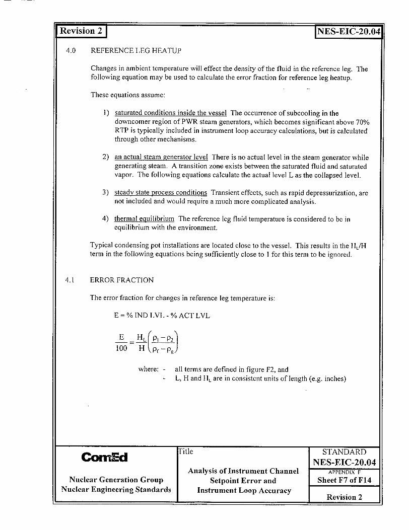
COnEd title STANDARD NES-EIC-20.04
Analysis of Instrument Channel APPENDIX F
Nuclear Generation Group Setpoint Error and Sheet F7 of F14 Nuclear Engineering Standards Instrument Loop Accuracy Revision 2
Revision 2 INES-EIC-20.04
4.0 REFERENCE LEG HEATUP
Changes in ambient temperature will effect the density of the fluid in the reference leg. The following equation may be used to calculate the error fraction for reference leg heatup.
These equations assume:
1) saturated conditions inside the vessel The occurrence of subcooling in the downcomer region of PWR steam generators, which becomes significant above 70% RTP is typically included in instrument loop accuracy calculations, but is calculated through other mechanisms.
2) an actual steam generator level There is no actual level in the steam generator while generating steam. A transition zone exists between the saturated fluid and saturated vapor. The following equations calculate the actual level L as the collapsed level.
3) steady state process conditions Transient effects, such as rapid depressurization, are not included and would require a much more complicated analysis.
4) thermal equilibrium The reference leg fluid temperature is considered to be in equilibrium with the environment.
Typical condensing pot installations are located close to the vessel. This results in the HL/H term in the following equations being sufficiently close to I for this term to be ignored.
4.1 ERROR FRACTION
The error fraction for changes in reference leg temperature is:
E = % IND LVL - % ACT LVL
100 H -p
where: - all terms are defined in figure F2, and - L, H and HL are in consistent units of length (e.g. inches)
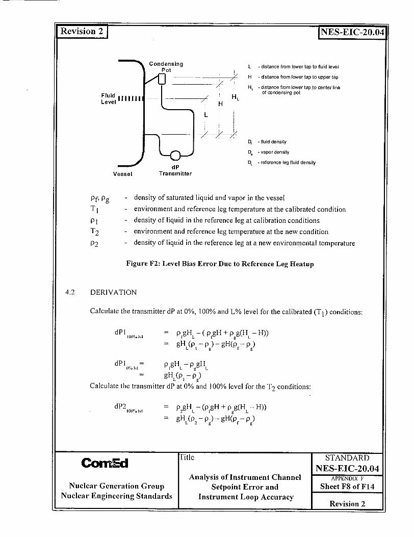
Revision 2
Fluid Level
L
H
H,
HL
// 7D,
D,- dP
Vessel Transmitter
- distance from lower tap to fluid level
- distance from lower tap to upper tap
- distance from lower tap to center line of condensing pot
- fluid density
- vapor density
- reference leg fluid density
- density of saturated liquid and vapor in the vessel - environment and reference leg temperature at the calibrated condition - density of liquid in the reference leg at calibration conditions - environment and reference leg temperature at the new condition - density of liquid in the reference leg at a new environmental temperature
Figure F2: Level Bias Error Due to Reference Leg Heatup
4.2 DERIVATION
Calculate the transmitter dP at 0%, 100% and L% level for the calibrated (T1 ) conditions:
dPI 100% lv
= pgH -(pgH + p g(H -H))
= gHi(P - p)-gH(p-p) ZSL f 9
dPI = pgH - p gH d 0%lv IV I L g L = gHL(P - p)
Calculate the transmitter dP at 0% and 100% level for the T2 conditions:
dP2 100I61v]
= pcgH -(prgH + p g(H - H))
= gH(p,) -- gH(p -p)
"d lTitle STANDARD onm d NES-EIC-20.04
Analysis of Instrument Channel APPENDIX F Nuclear Generation Group Setpoint Error and Sheet F8 of F14
Nuclear Engineering Standards Instrument Loop Accuracy Revision 2
I
INES-EIC-20.04
Pfp Pg TI
PI T2 P2
/
H L

V I
dP2 0% IV[
= prgH - p gH
= gHiL(p_,- p)
dP L
= (L/100)(dPlIo00 V [- dP loI V [) +dP lo %I
= (L/I00)(gHL(P - p)- gH(pf p) -g(p p)) +gHL(po - pg)
= gH(p- p)-(LgH/I00)(p--p)
This derivation uses a different, but more realistic concept. Starting with the indicated level that we observe, the actual level is calculated by including the effect of changes in reference leg density. Since level vs. dP is a linear relationship, a ratio is used to determine the actual level. Figure F3 will help in visualizing the required ratio.
actual% levelO
dP
level 100
I --------- I ----------- I dP20% dPL dP2 0% 100%
Figure F3, % Level vs. dP
ACT LVL - 0% 100% - 0/
dPL -- P2 0% dP2 1 /0 - dP2 0%
ACT LVL= dPL -dP2°1 xl00 dP21I 0o/, - dP2 0/o
The indicated level is equal to the calibrated dP, therefore:
• •'!- Title STANDARD COM EU NES-EIC-20.04
Analysis of Instrument Channel APPENDIX F
Nuclear Generation Group Setpoint Error and Sheet F9 of F14 Nuclear Engineering Standards Instrument Loop Accuracy FRevision 2
Revision 2 1 INES-EIC-20.04
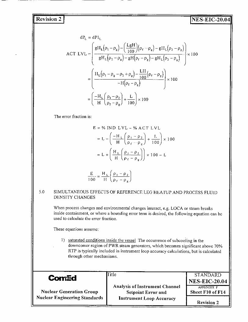
I
Revision2
dPL = dP1L
ACT LVL =
-HL +-L x+ 00 t, H j I-xlOO
The error fraction is:
E= %IND LVL-%ACT LVL
= L- -HL Pl P2 L 0 0
H f Pg +To
E H L P1-P21 100 H pf -pg
5.0 SIMULTANEOUS EFFECTS OF REFERENCE LEG HEATUP AND PROCESS FLUID DENSITY CHANGES
When process changes and environmental changes interact, e.g. LOCA or steam breaks inside containment, or where a bounding error term is desired, the following equation can be used to calculate the error fraction.
These equations assume:
1) saturated conditions inside the vessel The occurrence of subcooling in tile downcomer region of PWR steam generators, which becomes significant above 70% RTP is typically included in instrument loop accuracy calculations, but is calculated through other mechanisms.
"l Nitle STANDARD NES-EIC-20.04
Analysis of Instrument Channel APPENDIX F
Nuclear Generation Group Setpoint Error and Sheet F10 of F14 Nuclear Engineering Standards Instrument Loop Accuracy Revision 2
INES-EIC-20.04
-x 100
x 100

U, I
Revision2j NES-EIC-20.04O
2) an actual steam generator level There is no actual level in the steam generator while generating steam. A transition zone exists between the saturated fluid and saturated vapor. The following equations calculate the actual level L as the collapsed level.
3) steady state process conditions Transient effects, such as rapid depressurization, are not included and would require a much more complicated analysis.
4) thermal equilibrium The reference leg fluid temperature is considered to be in equilibrium with the environment.
Typical condensing pot installations are located close to the vessel. This results in the HL/H term in the following equations being sufficiently close to 1 for this term to be ignored.
5.1 ERROR FRACTION
E=%IND LVL-%ACTLVL
E HL_ L - PL2 - g + Pg2) L (Pf2 g
100 H ( f I -Pg H ( Pf, -Pgl
where: - all terms are defined in figure F4, and L, H and HL are in consistent units of length (e.g. inches)
itle STANDARD NES-EIC-20.04
Analysis of Instrument Channel APPENDIX F Nuclear Generation Group Setpoint Error and Sheet FlI of F14
Nuclear Engineering Standards Instrument Loop Accuracy Revision 2 ReiJo
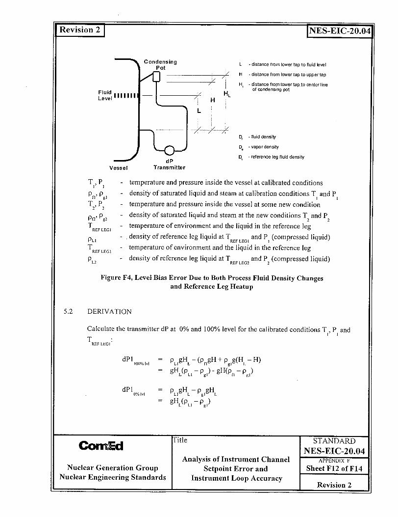
-- - - U §
Fluid Level 1i1111
L
H
H,
HL H
D,
Oý Dý
___ dP Vessel Transmitter
INES-EIC-20.04
- distance from lower tap to fluid level
- distance from lower tap to upper tap
- distance from lower tap-to center line of condensing pot
- fluid density
- vapor density
- reference leg fluid density
T, P - temperature and pressure inside the vessel at calibrated conditions
P l, P - density of saturated liquid and steam at calibration conditions T and P T, P - temperature and pressure inside the vessel at some new condition PP_, pg - density of saturated liquid and steam at the new conditions T and P T - temperature of environment and the liquid in the reference leg
REF LEGI
PLI - density of reference leg liquid at T and P (compressed liquid) T - temperature of environment and the liquid in the reference leg REF LEG2
PL2 - density of reference leg liquid at T REF LEG2 and P. (compressed liquid)
Figure F4, Level Bias Error Due to Both Process Fluid Density Changes and Reference Leg Heatup
5.2 DERIVATION
Calculate the transmitter dP at 0% and 100% level for the calibrated conditions T,, P and
T REF LEG I
dIP0oolvl = PLI gHL-(PfgH + pg]g(HL-- H) = gH (P -- Hp 1) -gH(pf - )
dPl g -g OL/ l vL~ g L P g l g H LP
gHcL -- gi = gH L(P L - Pgi)
n!d Title STANDARD CitCill NES-EIC-20.04
Analysis of Instrument Channel APPENDIX F Nuclear Generation Group Setpoint Error and Sheet F12 of F14
Nuclear Engineering Standards Instrument Loop Accuracy Revision 2
Revision 2
!
A
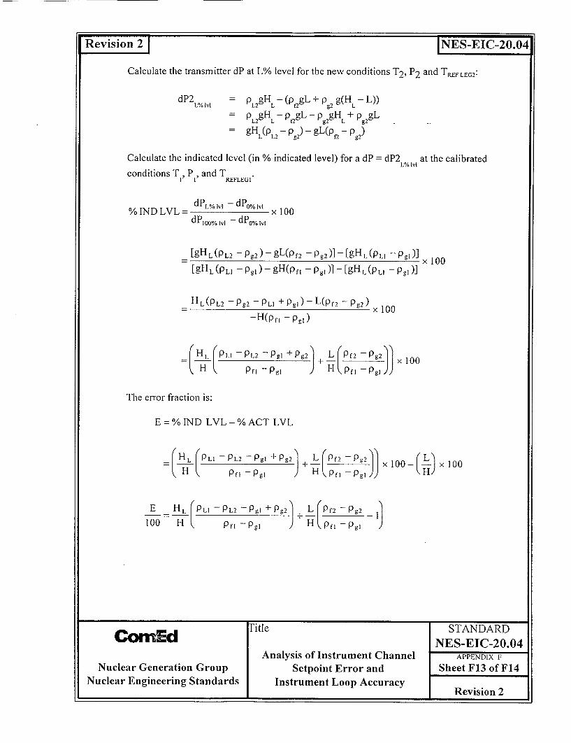
I i
Calculate the transmitter dP at L% level for the new conditions T2 , P2 and TREF LEG2:
OHLvl = L- (p gL + p g(H - L)) dP2 L% poH -2'L V g,)
P 2gH -p pgL - p gH +p PggL L2 L 02 g) L g
= gH(P - pg2 ) - gL(pf2 - pg2)
Calculate the indicated level (in % indicated level) for a dP = dP2 at the calibrated L% lvi
conditions T, P, and T REFLEGI
% IND LVL -dPLI1,l - x 100 dPoovo M -dPOIvI
[gHi(PL) - Pg2) -gL(pf) - Pg)] - [gHi(PL- Pgi)] -- -" " x 100
[gHL(PL1 - Pgl ) - gH(pf -pg)] - [gHl(PL1 - PgA)]
HL(PL2 -- Pg2 - PLI + pg, )- L(Pf2 - Pg2) -H(pn - Pgl)
HL PLI -P2 -PgI +P- g
H ~PfV -PgI+ _L______Pg x 100
The error fraction is:
E=% IND LVL-%ACT LVL
HL(PLI -PL2 -PgI + Pg2 +L (Pf2 -Pg2 x 0 - x10 rH I fL I-I- H (100---x(00 K Pfl Pgi Pfl Pgi 'JH
E H L PLI -P-2 -PgI + Pg2 +L (Pf2 -Pg2
100 H ( P1' - PgI H K pf, - pI1
Title STANDARD CbrnEd NES-EIC-20.04 Analysis of Instrument Channel APPENDIX F
Nuclear Generation Group Setpoint Error and Sheet F13 of F14 Nuclear Engineering Standards Instrument Loop Accuracy Revision 2
Revision 2 1 INES-EIC-20.041
Zevision 2 I INES-EIC-20.04
6.0 REFERENCE LEG BOILING
In addition to process and reference leg density changes, boiling could conceivable occur in the reference leg due to rapid depressurization. Boiling or other gases coming out of solution in the reference leg would result in a large level error for a short period of time.
For PWR plants, both pressurizer level and steam generator level could be effected by reference leg boiling. Analysis of chapter 15 events and containment analysis for CornEd PWR stations indicate that no reference leg boiling is expected that would effect a protection setpoint. For pressurizer level setpoints, the RCS pressure is not expected to decrease below 1400 psig during a transient which prevents reference leg boiling. The accidents that rely on steam generator low level setpoints are not expected to experience depressurization at a rate that would result in reference leg boiling.
NOTE: transients that could result in hydrogen coming out of solution in the pressurizer reference leg are not currently addressed in the setpoint analyses.
For BWR plants, the possibility of reference leg boiling and reactor vessel level errors due to dissolved gasses coming out of solution has been addressed. The RVLIS/Backfill modifications have been installed in accordance with Generic Letter 92-04, Resolution of the Issues Related to Reactor Vessel Water Level Instrumentation in BWRs Pursuant to I 0CFR50.54(f). Setpoint accuracy calculations and reactor vessel level scaling calculations incorporate the effects of this modification on the associated reactor protection setpoints.
7.0 References
7.1 CAE-92-189/CCE-92-201/CWE-92-214, Commonwealth Edison Company, Zion/Byron/Braidwood Stations, S/G Water Level PMA Term Inaccuracies, dated 6/18/92
7.2 CWE-79-26, Commonwealth Edison Company, Zion Station, NRC IE Bulletin 79-21, dated 8/29/79
7.3 NRC IE Bulletin 79-21, Temperature Effects on Level Measurements
7.4 "Delta-P Level Measurement Systems", Lang, Glenn E. And Cunnigham, James P., Instrumentation, Controls and Automation in the Power Industry, vol. 34, Proceeding of the 34th Power Instrument Symposium, June 1991
7.5 Generic Letter 92-04, Resolution of the Issues Related to Reactor Vessel Water Level Instrumentation in BWRs Pursuant to IOCFR50.54(f)
Com~d Title STANDARD NES-EIC-20.04
Analysis of Instrument Channel APPENDIX F
Nuclear Generation Group Setpoint Error and Sheet F14 of F14 Nuclear Engineering Standards Instrument Loop Accuracy Revision 2

Revision 21 INES-EIC-20.04
APPENDIX G
DELTA-P MEASUREMENTS EXPRESSED IN FLOW UNITS
Latest Revision indicated by a bar in right hand margin.
Title STANDARD CQ rnEd NES-EIC-20.04
Analysis of Instrument Channel APPENDIX G Nuclear Generation Group Setpoint Error and Sheet GI of G9
Nuclear Engineering Standards Instrument Loop Accuracy Revision 2
Revision 2 I I

Revision 2
1.0 INTR
INES-EIC-20.04
ODUCTION
Propagation of errors and uncertainties through a non-linear device results in output errors and uncertainties that are a function of the input value. In the case of the typical flow vs. dP relationship, an approximation can be derived for the square root/square function. This appendix provides an equation that can be used to convert between errors in % dP and errors in % full scale.
Orifices, nozzles and venturies are typically provided with their flow uncertainty expressed as a % of full scale dP. This uncertainty is the same anywhere within the measured span. As an example, an orifice that has a full span of 100 in.WC and is specified to be accurate to ±-1% full span, will have an uncertainty of±l inch of water anywhere in the measured span. Since dP is a function of flow squared, this cannot be said for errors expressed in terms of flow, % flow or % flow span. The flow error will depend on the corresponding value of flow.
2.0 DERIVATION
Since dP is proportional to flow squared:
(FN)2
dPN (Eq. GI)
where N = Nominal Flow
Taking the partial derivative and solving for 9FN:
2 FNaFN =
aFN =
adPN (OdPN)/(2FN)
Similarly, the error at a point (not in %) is:
FN _ dPN _ dPN FN 2(FN ) 2 2dPN
and from equation G 1:dPN
dPMAX
(FN )2
(FMAX )
where: MAX = maximum flow
PrM lTitle STANDARD COrnEd NES-EIC-20.04
Analysis of Instrument Channel APPENDIX G Nuclear Generation Group Setpoint Error and Sheet G2 of G9
Nuclear Engineering Standards Instrument Loop Accuracy Revision 2
(Eq. G2)
(Eq. G3)

Revision 2 1
The transmitter dP error is defined by:
adPNý adPKý = % error in full scale dP (% FS dP)
Therefore:
dP (%FS dP"
aFN _dPN MAx 100 0
F N 2dPN 2dPM' ~ N 1
, MAX)
%FS dP(FMAX
(2)(100)
The error in flow units is obtained by solving for aFN: )2 D FN F(% FS dP)<MAX D
(2)(100)
This can be rearranged to represent the error in % nominal flow:
aFN x 100 °F -dPFMAx 2
N '\ FN)
From equation G7, the error in % full span can be derived:
9 OFN (FM x=
r x(100
(FMAX )(2)(100)
(.°%FS dP ('FMAX/ -~ 2 )F)
CtoEd Title STANDARD NES-EIC-20.04
Analysis of Instrument Channel APPENDIX G
Nuclear Generation Group Setpoint Error and Sheet G3 of G9 Nuclear Engineering Standards Instrument Loop Accuracy
Revision 2
INES-EIC-20.04
(Eq. G4)
(Eq. G5)
(Eq. G6)
(Eq. G7)
(Eq. G8)
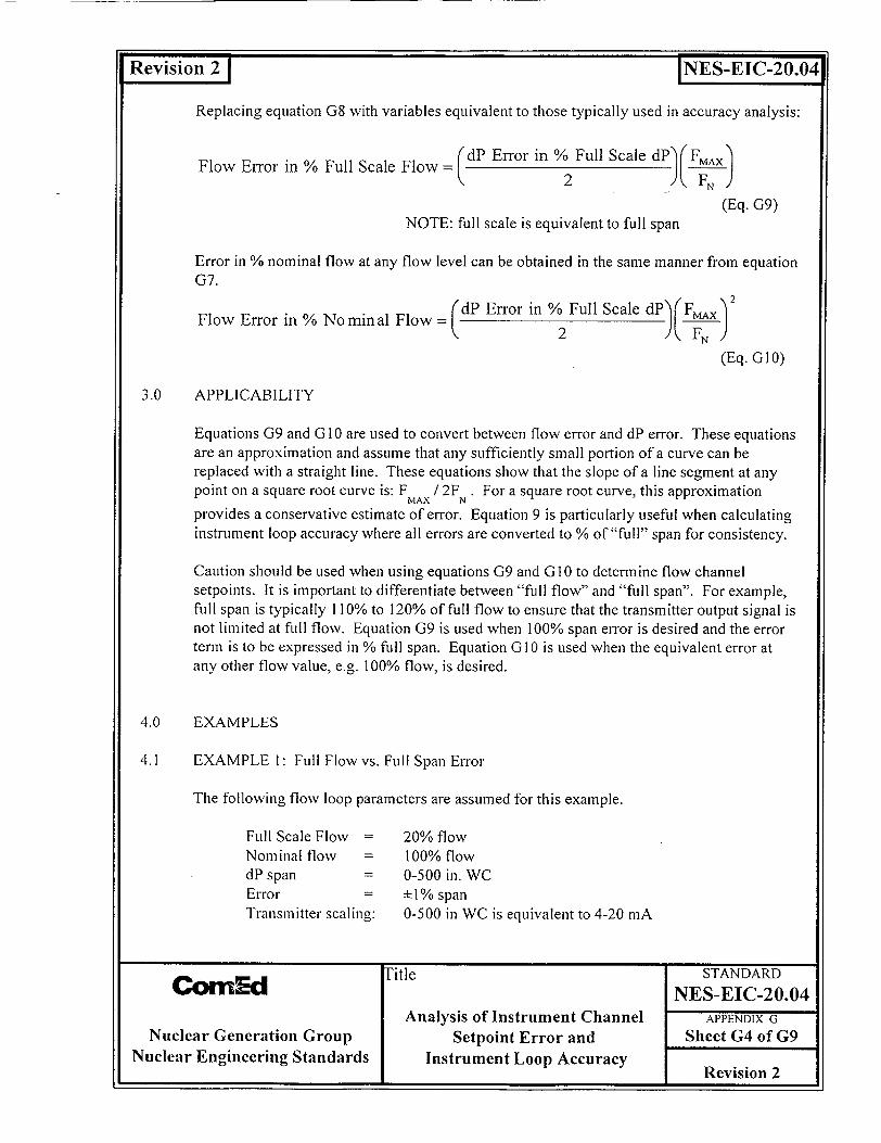
21 INES-EIC-20.04
Replacing equation G8 with variables equivalent to those typically used in accuracy analysis:
Flow Error in % Full Scale Flow C dP Error in % Full Scale dP')(FMAx] 2 A-FN
(Eq. G9)NOTE: full scale is equivalent to full span
Error in % nominal flow at any flow level can be obtained in the same manner from equation G7.
Flow Error in % Nominal Flow = (dP Error in % Full Scale dP)rFMAX
(Eq. G 1O)
3.0 APPLICABILITY
Equations G9 and G 10 are used to convert between flow error and dP error. These equations are an approximation and assume that any sufficiently small portion of a curve can be replaced with a straight line. These equations show that the slope of a line segment at any point on a square root curve is: F / 2F . For a square root curve, this approximation MAX N
provides a conservative estimate of error. Equation 9 is particularly useful when calculating instrument loop accuracy where all errors are converted to % of "full" span for consistency.
Caution should be used when using equations G9 and G10 to determine flow channel setpoints. It is important to differentiate between "full flow" and "full span". For example, full span is typically 110% to 120% of full flow to ensure that the transmitter output signal is not limited at full flow. Equation G9 is used when 100% span error is desired and the error term is to be expressed in % full span. Equation G10 is used when the equivalent error at any other flow value, e.g. 100% flow, is desired.
4.0 EXAMPLES
4.1 EXAMPLE 1: Full Flow vs. Full Span Error
The following flow loop parameters are assumed for this example.
Full Scale Flow =
Nominal flow = dP span = Error Transmitter scaling:
20% flow 100% flow 0-500 in. WC ± 1% span 0-500 in WC is equivalent to 4-20 mA
"!!!Aitle STANDARD Cbrncd NES-EIC-20.04
Analysis of Instrument Channel APPENDIX G
Nuclear Generation Group Setpoint Error and Sheet G4 of G9 Nuclear Engineering Standards Instrument Loop Accuracy Revision
2

Revision 2 1
NOTE: typical orifice and nozzle span errors are provided as an error in dP span which is constant over the entire dP span.
4.1.1 Find the error in % flow at 100% flow
From section 4. 1:
F = 120% MAX
F = 100% N
error in % full scale dP = 1% dP span
Use equation G10 for nominal flow error determination.
Error% Nominal Flow = V dP Error in % Full Scale dP.(FMAX 2 -T,7N)
= ±0.72% flow at 100% flow
4.1.2 Find the error at full span (120% flow).
F = 120% MAX
F = 100% N
error in % full scale dP =±-1% dP span
Use equation G9 for full span error determination.
Error% Full Scale FlowdP Error in % Full Scale dP) FMAx
= ±0.6% flow span
Title STANDARD CornEd NES-EIC-20.04
Analysis of Instrument Channel APPENDIX G Nuclear Generation Group Setpoint Error and Sheet G5 of G9
Nuclear Engineering Standards Instrument Loop Accuracy Revision 2
INES-EIC-20.04
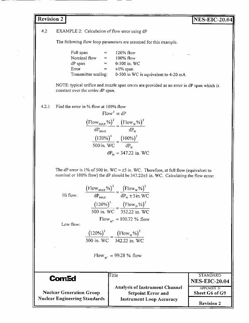
Revision2
4.2 EXAMPLE 2: Calculation of flow error using dP
The following flow loop parameters are assumed for this example.
Full span =
Nominal flow = dP span = Error Transmitter scaling:
120% flow 100% flow 0-500 in. WC +1% span 0-500 in WC is equivalent to 4-20 mA
NOTE: typical orifice and nozzle span errors are provided as an error in dP span which is constant over the entire dP span.
4.2.1 Find the error in % flow at 100% flow
Flow 2 oc dP
(Flowmx %)2 _ (FlowN %)2
dPMAX dPN
(120%)2 (100%)2
500in. WC dPN
dPN = 347.22 in. WC
The dP error is 1% of 500 in. WC = ±5 in. WC. Therefore, at full flow (equivalent to nominal or 100% flow) the dP should be 347.22±5 in. WC. Calculating the flow error:
Hi flow:
Low flow:
(FlowMAX%)2
dPMAX
(FlowN %)2
dPN 5in.WC
(120%)2 _ (F'lowN%) 2
500 in. WC 352.22 in. WC
Flow N= 100.72 % flow
(120%)2 (FlowN
500 in. WC 342.22 in. WC
Flow = 99.28 % flow
Title STANDARD CornEd NES-EIC-20.04
Analysis of Instrument Channel APPENDIX G Nuclear Generation Group Setpoint Error and Sheet G6 of G9
Nuclear Engineering Standards Instrument Loop Accuracy FRevision 2
INES-EIC-20.04

Revision 2 1 INES-EIC-20.04
Therefore the flow error is ±0.72% flow at full flow. This is consistent (to 2 decimal places) with the error calculated using the approximation formula in step 4.1.1.
4.2.2 Find the error in % full span at 100% flow
When using % full span to combine errors, the error at 100% flow must also be expressed in terms of% full span.
Full flow = (100% flow)(100% span / 120% flow) = 83.33% of full span
From 4.2.1, the flow error is ±0.72% flow at full flow, which is equivalent to 100±0.72% flow. Converting this to % of span:
(100 + 0.72)(100% span/ 120% flow) = 83.93% full span
(100 - 0.72)(100% span / 120% flow) = 82.73% full span
The deviation from full flow as a % of span is: 83.93% span - 83.33% span = 0.6% span and 83.33% span - 82.73% span = 0.6% span. Therefore, the nominal or 100% flow in terms of % full span is equivalent to 83.33±0.6% full span, which is consistent with step 4.1.2.
4.3 FLOW ERROR AT LOW FLOWS
As shown in step 4.2, the approximation and the actual flow errors are expected to be relatively close when the nominal flow is close to full flow. Since errors as a % of span increase as flow decreases, the approximation becomes increasingly conservative at lower flows. Therefore, at low flows or when the exact flow error is desired, the dP method should be used to calculate flow error.
4.4 EXAMPLE 3: Error at Low flows
The flow error associated with a low flow trip at 30% flow is required. Using the same values in steps 4.1 and 4.2:
itle STANDARD CornEd NES-EIC-20.04
Analysis of Instrument Channel APPENDIX G Nuclear Generation Group Setpoint Error and Sheet G7 of G9
Nuclear Engineering Standards Instrument Loop Accuracy Revision 2
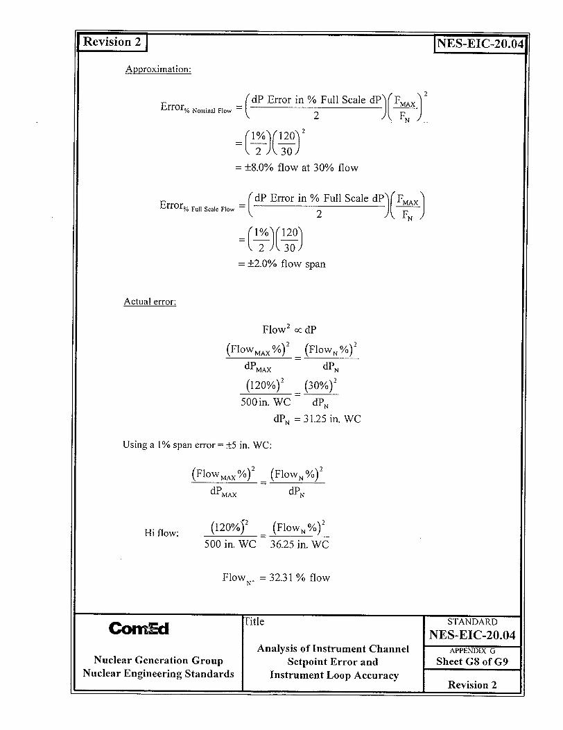
Revision 21
Approximation:
INES-EIC-20.04
=(dP Error in% Full Scale dPFmx
2 N3
= ±8.0% flow at 30% flow
(dP Error in % Full Scale dP.)(FmAx) = 2 \--FN
=± % fs120 a
= ±2.0% flow span
Actual error:
Flow 2 oc dP
(FIowMAX %)2 (FlOWN %)2
dPMAX dPN
(120%)2
500 in. WC(30%)-2
dPN
dPN =31.25 in. WC
Using a 1% span error = ±5 in. WC:
(FlowMAX %)2
dPMAX
(FlowN %)2
dPN
Hi flow: (120%j 2 _ (FlowN %)2
500 in. WC 36.25 in. WC
Flow = 32.31 % flow
Title STANDARD CornEd NES-EIC-20.04 Analysis of Instrument Channel APPENDIX G
Nuclear Generation Group Setpoint Error and Sheet G8 of G9 Nuclear Engineering Standards Instrument Loop Accuracy Revision 2
Error% Nnminal Flo•v
Error* Full Scale Flow
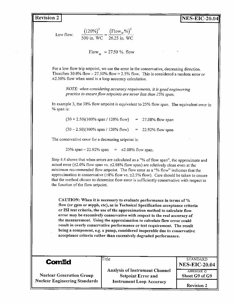
Revision 2 1 [NES-EIC-20.04
Low flow: (120%)2 (FloW %) 2
500 in. WC 26.25 in. WC
Flow N =2750 %. flow
For a low flow trip setpoint, we use the error in the conservative, decreasing direction. Therefore 30.0% flow - 27.50% flow = 2.5% flow. This is considered a random error or ±2.50% flow when used in a loop accuracy calculation.
NOTE.- when considering accuracy requirements, it is good engineering practice to ensure flow setpoints are never less than 25% span.
In example 3, the 30% flow setpoint is equivalent to 25% flow span. The equivalent error in % span is:
(30 + 2.50)(100% span / 120% flow) = 27.08% flow span
(30 - 2.50)(100% span / 120% flow) = 22.92% flow span
The conservative error for a decreasing setpoint is:
25% span - 22.92% span = +2.08% flow span.
Step 4.4 shows that when errors are calculated as a "% of flow span", the approximate and actual error (±2.0% flow span vs. ±2.08% flow span) are relatively close even at the minimum recommended flow setpoint. The flow error as a "% flow" indicates that the approximation is conservative (±8% flow vs. ±2.5% flow). Care should be taken to ensure that the method chosen to determine flow error is sufficiently conservative with respect to the function of the flow setpoint.
CAUTION: When it is necessary to evaluate performance in terms of % flow (or gpm or mpph, etc), as in Technical Specification acceptance criteria or ISI test criteria, the use of the approximation method to calculate flow error may be excessively conservative with respect to the real accuracy of the measurement. Using the approximation to calculate flow error could result in overly conservative performance or test requirement. The result being a component, e.g. a pump, considered inoperable due to conservative acceptance criteria rather than excessively degraded performance.
Title STANDARD COrnEd NES-EIC-20.04
Analysis of Instrument Channel APPENDIX G Nuclear Generation Group Setpoint Error and Sheet G9 of G9
Nuclear Engineering Standards Instrument Loop Accuracy Revision 2
- - - I I
Revision 2 1 INES-EIC-20.04
APPENDIX H
CALCULATION OF EQUIVALENT POINTS ON NON-LINEAR SCALES
Latest Revision indicated by a bar in right hand margin.
Title STANDARD CornEd NES-EIC-20.04
Analysis of Instrument Channel APPENDIX H Nuclear Generation Group Setpoint Error and Sheet H1 of H6
Nuclear Engineering Standards Instrument Loop Accuracy Revision 2
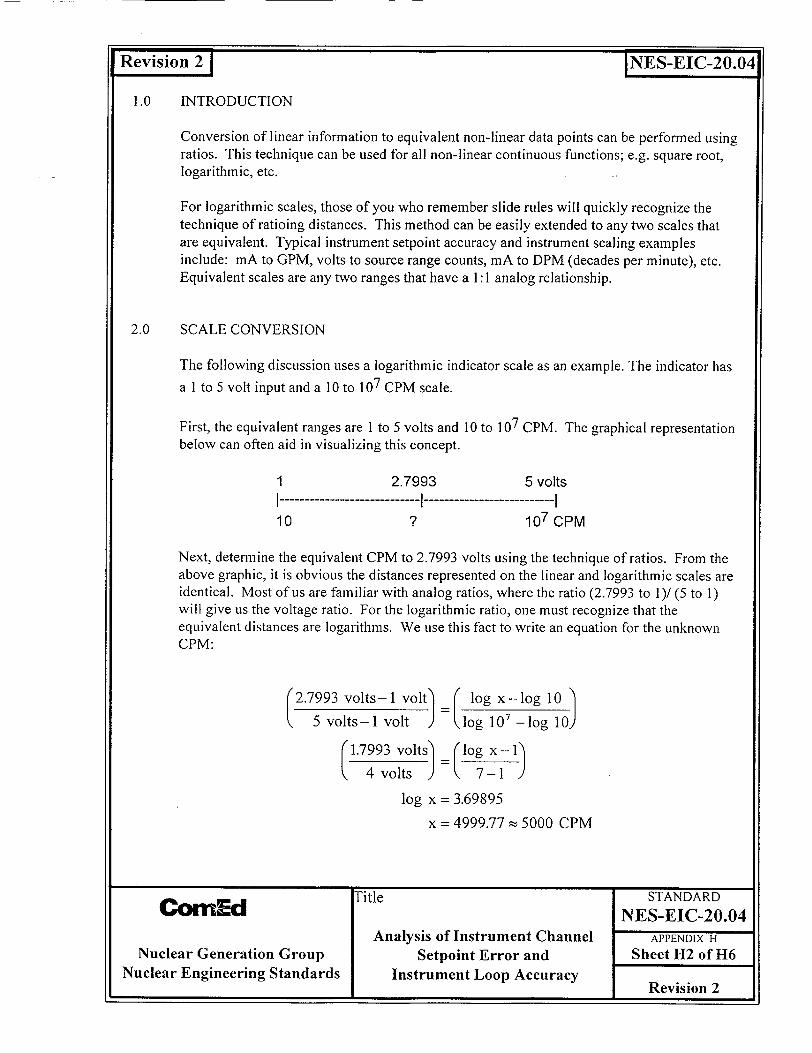
Revision 2 1 INES-EIC-20.04
1.0 INTRODUCTION
Conversion of linear information to equivalent non-linear data points can be performed using ratios. This technique can be used for all non-linear continuous functions; e.g. square root, logarithmic, etc.
For logarithmic scales, those of you who remember slide rules will quickly recognize the technique of ratioing distances. This method can be easily extended to any two scales that are equivalent. Typical instrument setpoint accuracy and instrument scaling examples include: mA to GPM, volts to source range counts, mA to DPM (decades per minute), etc. Equivalent scales are any two ranges that have a 1: 1 analog relationship.
2.0 SCALE CONVERSION
The following discussion uses a logarithmic indicator scale as an example. The indicator has
a I to 5 volt input and a 10 to 107 CPM scale.
First, the equivalent ranges are I to 5 volts and 10 to 107 CPM. The graphical representation below can often aid in visualizing this concept.
1 2.7993 5 voltsI ------------ ----------- I10 107 CPM
Next, determine the equivalent CPM to 2.7993 volts using the technique of ratios. From the above graphic, it is obvious the distances represented on the linear and logarithmic scales are identical. Most of us are familiar with analog ratios, where the ratio (2.7993 to 1)/ (5 to 1) will give us the voltage ratio. For the logarithmic ratio, one must recognize that the equivalent distances are logarithms. We use this fact to write an equation for the unknown CPM:
2.7993 volts-I volt) 5 volts-I volt )
C log x-log 10 .log 107 -•og 10)
4volts ) ý 7-1
log x = 3.69895
x = 4999.77 • 5000 CPM
on - Title STANDARD Cbrn~d NES-EIC-20.04
Analysis of Instrument Channel APPENDIX H Nuclear Generation Group Setpoint Error and Sheet H2 of H6
Nuclear Engineering Standards Instrument Loop Accuracy 6 t5 I-Revision 2

Reiso 2 IC-~
An alternate method to solve for log x:
log x = 3.69895
x = 103.69895 = 1 0o.69895 x i W
= 4.998 x 10³ • 5000 CPM
For this discussion, assume that the linear uncertainty is 2% of span. This is equivalent to:
2.7993 volts ± (2%(5 volts - 1 volt)) = 2.7993 ± 0.08 volts
Using the ratioing technique, it becomes a simple matter to find the equivalent CPM values for 2.8793 volts and 2.7919 volts. The +2% tolerance equations are provided below, followed by the completed graphic.
2.7993 volts-0.8 voltsI ( log x-log 10
5 volts-I volt ) = log 10- -log 10) (1.8793 volts) o x 4 vol)s 7-1
log x =3.81895
x = 6590.98 z 6591 CPM
1 2.7993
-2% +2% I 2.7193 2.8793 volts I--------------------- I ---------------- I ------------ I ---------------I 3793 6591 CPM I10 5"103 1
volts
07 CPM
Thus, for a linear input of I to 5 volts with an error of +2% of span, the equivalent uncertainty range at 5000 CPM is 3793 to 6591 CPM. As with all non-linear relationships, it is important to note that the uncertainty range is dependent on the point on the non-linear scale around which the uncertainty is calculated. In other words the +1591, -1207 CPM uncertainty range is only valid at 5000 CPM.
Title STANDARD CornEd NES-EIC-20.04
Analysis of Instrument Channel APPENDIX H
Nuclear Generation Group Setpoint Error and Sheet H3 of H6 Nuclear Engineering Standards Instrument Loop Accuracy Revision 2
Revision 2 1 INES-EIC-20.041
5
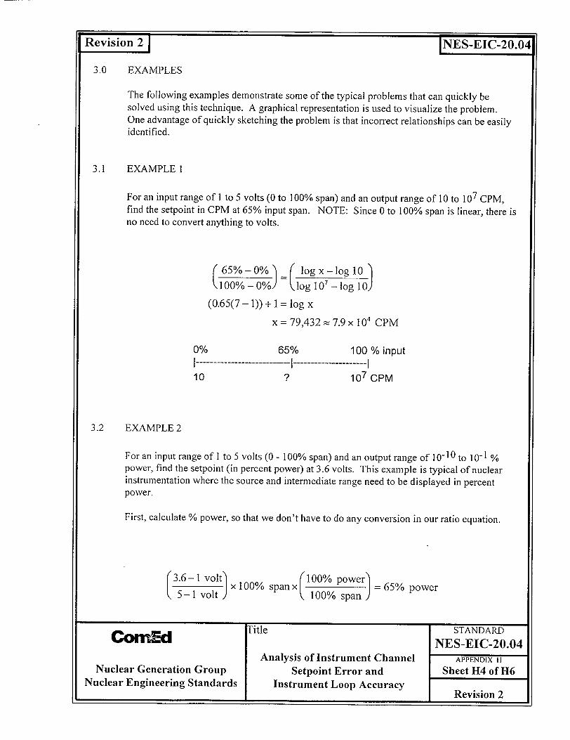
- - I m
INES-EIC-20.04
3.0 EXAMPLES
The following examples demonstrate some of the typical problems that can quickly be solved using this technique. A graphical representation is used to visualize the problem. One advantage of quickly sketching the problem is that incorrect relationships can be easily identified.
3.1 EXAMPLE 1
For an input range of I to 5 volts (0 to 100% span) and an output range of 10 to 107 CPM, find the setpoint in CPM at 65% input span. NOTE: Since 0 to 100% span is linear, there is no need to convert anything to volts.
100% -0%) =U lgi ;-log0-0) (0.65(7 - 1)) + 1 = log x
x = 79,432 - 7.9 x 10⁴ CPM
0% 65% 100 % inputI ------------ I --------- I 10 ? 107 CPM
3.2 EXAMPLE 2
For an input range of I to 5 volts (0 - 100% span) and an output range of 10-10 to 10-1 % power, find the setpoint (in percent power) at 3.6 volts. This example is typical of nuclear instrumentation where the source and intermediate range need to be displayed in percent power.
First, calculate % power, so that we don't have to do any conversion in our ratio equation.
.6-1 volt (100% power x 100% = 65% power
Title STANDARD CornEd NES-EIC-20.04
Analysis of Instrument Channel APPENDIX H
Nuclear Generation Group Setpoint Error and Sheet H4 of H6 Nuclear Engineering Standards Instrument Loop Accuracy Revision 2
Revision2
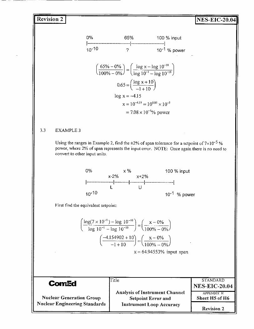
Revision 2 1 INES-EIC-20.04
0% 65% 100 % input I --------------------------- I --------------------- I 10-10 ? 10- 1 % power
(65%-0% 1 ( logx-logl0-'°
100%- 0%) =Kiog i0' -log 10,0)
0.65 1 -0
log x =-4.15
x 10-4.15 = 10°08) x 10
7.08 x 10⁻⁵% power
3.3 EXAMPLE 3
Using the ranges in Example 2, find the ±2% of span tolerance for a setpoint of 7x 10- 5 % power, where 2% of span represents the input error. NOTE: Once again there is no need to convert to other input units.
0% 100 % inputx-2% x+2%
SI ----- I ------ I -------- IL U
10-10 10-1% power
First find the equivalent setpoint:
log(7 x 10⁻⁵)-log 10-1'° x-0%
log 10-' -log 10`0 ) (100%-0%)
x4.154902+10 ( X-0% -1i+10 ) \ 100%- 0%)
x = 64.94553% input span
Title STANDARD CornEd NES-EIC-20.04
Analysis of Instrument Channel APPENDIX H
Nuclear Generation Group Setpoint Error and Sheet H5 of H6 Nuclear Engineering Standards Instrument Loop Accuracy
Revision 2

INES-EIC-20.04
Use the following ratio to solve for the upper limit (U).
(64.94553+2)-0% = 100% - 0% )
C log U-log 10-°1 -) logi -10('-lo 10 10)
0.6 6 94 53 3 = (log U + 10 9
U = 10-3974902 = 1.06 x 10⁻⁴% power
Solve for the lower limit (L).
U = 10-3.97492 = 1.06 x 10⁻⁴% power
As expected, non-linear scales result in non-symmetrical upper and lower values for an equivalent symmetrical input error. When evaluating the accuracy of a single point (e.g. bistable setpoint or EOP required actuation point), you can use the limit associated with the direction of the process change. Thus an increasing setpoint would use U and a decreasing setpoint would use L for calculating accuracy.
When calculating accuracy for a point on an indicator scale, the accuracy values are used in 2 different ways. When calibrating the indicator the calibration limits can use the specific L and U values for each cardinal point. When providing accuracy values to a plant operator or other individual that is using the indicator to monitor a plant process condition, it is usually inconvenient to list asymmetric limits. In this case it is conservative to describe accuracy as +U or ±L, whichever is larger.
In order to use the ratio technique for other non-linear functions, compare (ratio) the equivalent scalar distances of each range. Thus with square root/square relationships, such as flow (GPM, CFM, etc.) or percent of flow, the ratio is obtained by taking the square root or square of the corresponding linear value.
L=J Title STANDARD NES-EIC-20.04
Analysis of Instrument Channel APPENDIX 1
Nuclear Generation Group Setpoint Error and Sheet H6 of H6 Nuclear Engineering Standards Instrument Loop Accuracy t3 I [ Revision 2

Iso jNS-I-00
APPENDIX I
NEGLIGIBLE UNCERTAINTIES
Latest Revision indicated by a bar in right hand margin.
Title STANDARD CounEd NES-EIC-20.04 Analysis of Instrument Channel APPENDIX I
Nuclear Generation Group Setpoint Error and Sheet I1 of 16 Nuclear Engineering Standards Instrument Loop Accuracy In Revision 2
Revision 2 1 INES-EIC-20.04
Revision 2 1 INES-EIC-20.04
1.0 INTRODUCTION
The errors and uncertainties listed in this appendix have historically been found to be negligible under normal operating conditions. If the individual preparing an instrument loop accuracy calculation determines that the specific conditions apply, then these errors and uncertainties do not have to be evaluated in the calculation.
2.0 NEGLIGIBLE UNCERTAINTIES
2.1 Radiation Effects
The effects of normal radiation are small and accounted for in the periodic calibration process. Outside of containment there is not a creditable increase in radiation during normal operation. The uncertainty introduced by radiation effects on components is considered to be negligible.
If an as-found/as-left analysis has been performed based on historical calibration data, the radiation effect is considered to be included in the drift analysis results.
2.2 Humidity Effects
The uncertainty introduced by humidity effects during normal conditions is not typically addressed in vendor literature. Therefore humidity effects are considered to be negligible unless the manufacturer specifically mentions humidity effects in the applicable technical manual. The effects of changes in humidity on the components is considered to be calibrated out on a periodic basis. A condensing environment is regarded as an abnormal event which will require maintenance to the equipment. Humidities below 10% are expected to occur very infrequently and are not considered.
If an as-found/as-left analysis has been performed based on historical calibration data, the humidity effect is assumed to be included in the drift analysis results.
2.3 Power Supply Effects
It is expected that regulated instrument power supplies have been designed to function within manufacturer's required voltage limits. The variations of voltage and frequency are expected to be small and the power supply voltage and frequency uncertainties are considered to be negligible with respect to other error terms.
ritle STANDARD COrnEd NES-EIC-20.04
Analysis of Instrument Channel APPENDIX I
Nuclear Generation Group Setpoint Error and Sheet 12 of 16 Nuclear Engineering Standards Instrument Loop Accuracy Revision 2
Revision 2 1 INES-EIC-20.04
If an as-found/as-left analysis has been performed based on historical calibration data, the power supply voltage and frequency effects are assumed to be included in the drift analysis results.
2.4 Calibration Standard Error (STD)
The calibration standards used by the station to maintain and calibrate station M&TE are expected to be maintained to manufacturer's specifications. These calibration standards are more accurate than the station M&TE by a ratio greater than 4:1. Therefore, the effects of the calibration standard error are considered to be negligible with respect to other error terms.
2.5 Seismic/Vibration Effects
For normal errors, seismic events less than or equal to an OBE are considered to cause no permanent shift in the input/output relationship of the device. For seismic events greater than an OBE, it should be verified that the affected instrumentation is recalibrated prior to any subsequent accident to negate any permanent shift which may be resulted from a post seismic shift.
Unlike Seismic effects, Vibration effects may not always be calibrated out or included in the statistical drift. Consideration must be made of the "normal operating" versus "calibration" conditions. If the relative vibration conditions of these two states is not the same, then the vibration effect must be considered. This effect is not calibrated out or included in the historical calibrations data.
If an as-found/as-left analysis has been performed based on historical calibration data, the vibration effect is considered to be included in the drift analysis results, if the normal operation conditions and the calibration conditions are similar.
2.6 Lead Wire Effects
Since the resistance of a wire is equal to the resistivity times the length divided by the cross sectional area, the very small differences in the length of wires between components does not contribute any significant resistance differences between wires. Therefore, the effect of lead wire resistance differences is considered negligible, except for RTDs and thermocouples.
If a system design requires that lead wire effects be considered as a component of uncertainty, that requirement must be included in the design basis. It is assumed that the general design standard is to eliminate lead wire effects as a concern in both equipment design and installation. Failure to do so is a design fault that should be corrected.
The lead wire effects for RTDs and thermocouples must be considered separately and must be evaluated for each specific application.
Title STANDARD ComEd NES-EIC-20.04
Analysis of Instrument Channel APPENDIX I
Nuclear Generation Group Setpoint Error and Sheet 13 of 16 Nuclear Engineering Standards Instrument Loop Accuracy Revision 2
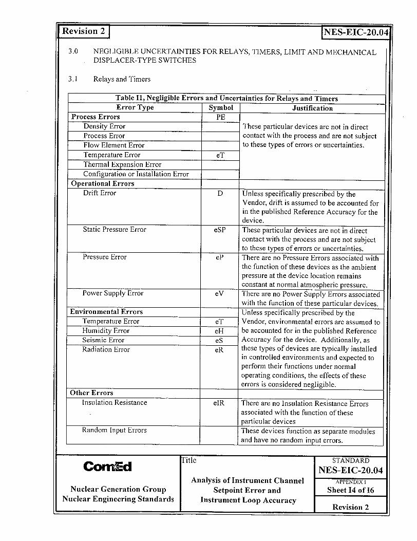
I . . . .M
Revisio
3.0
INS-IC -2O.O41
NEGLIGIBLE UNCERTAINTIES FOR RELAYS, TIMERS, LIMIT AND MECHANICAL DISPLACER-TYPE SWITCHES
3.1 Relays and Timers
Table II, Negligible Errors and Uncertainties for Relays and Timers Error Type Symbol Justification
Process Errors PE Density Error These particular devices are not in direct Process Error contact with the process and are not subject Flow Element Error to these types of errors or uncertainties. Temperature Error eT Thermal Expansion Error Configuration or Installation Error
Operational Errors Drift Error D Unless specifically prescribed by the
Vendor, drift is assumed to be accounted for in the published Reference Accuracy for the device.
Static Pressure Error eSP These particular devices are not in direct contact with the process and are not subject to these types of errors or uncertainties.
Pressure Error eP There are no Pressure Errors associated with the function of these devices as the ambient pressure at the device location remains constant at normal atmospheric pressure.
Power Supply Error eV There are no Power Supply Errors associated with the function of these particular devices.
Environmental Errors Unless specifically prescribed by the Temperature Error eT Vendor, environmental errors are assumed to Humidity Error eH be accounted for in the published Reference Seismic Error eS Accuracy for the device. Additionally, as Radiation Error eR these types of devices are typically installed
in controlled environments and expected to perform their functions under normal operating conditions, the effects of these errors is considered negligible.
Other Errors Insulation Resistance elR There are no Insulation Resistance Errors
associated with the function of these particular devices
Random Input Errors These devices function as separate modules and have no random input errors.
itle STANDARD COmEd NES-EIC-20.04 Analysis of Instrument Channel APPENDIX I
Nuclear Generation Group Setpoint Error and Sheet 14 of 16 Nuclear Engineering Standards Instrument Loop Accuracy
I I F Revision 2
,n2 1 ).041

VRevision 2 1 INES-EIC-20.04
3.2 Limit Switches
Table 12, Negligible Errors and Uncertainties for Limit SwitchesError Type Symbol Justification
Process Errors PE Density Error These particular devices are not in direct Process Error contact with the process and are not subject Flow Element Error to these types of errors or uncertainties.
Temperature Error eT Thermal Expansion Error Configuration or Installation Error
Operational Errors Drift Error D Unless specifically prescribed by the
Vendor, drift is not applicable for these type of devices.
Static Pressure Error eSP These particular devices are not in direct contact with the process and are not subject
to these types of errors or uncertainties. Pressure Error eP There are no Pressure Errors associated with
the function of these devices as the ambient pressure at the device location remains constant at normal atmospheric pressure.
Power Supply Error eV There are no Power Supply Errors associated with the function of these particular devices.
Environmental Errors Temperature Error eT Unless specifically prescribed by the Humidity Error eH Vendor, environmental errors are assumed to Seismic Error eS be accounted for in the published Reference Radiation Error eR Accuracy for the device.
Other Errors Insulation Resistance elR There are no Insulation Resistance Errors
associated with the function of these particular devices
Random Input Errors These devices function as separate modules
and have no random input errors.
0itle STANDARD COm11 NES-EIC-20.04
Analysis of Instrument Channel APPENDIX I
Nuclear Generation Group Setpoint Error and Sheet 15 of 16 Nuclear Engineering Standards Instrument Loop Accuracy evision 2
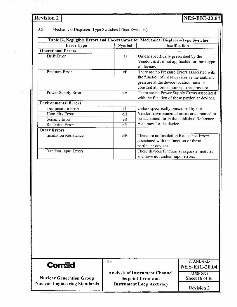
U I
Revision2i NES-EIC-20.04
3.3 Mechanical Displacer-Type Switches (Float Switches)
Table 12, Negligible Errors and Uncertainties for Mechanical Displacer-Type SwitchesError Type Symbol Justification
Operational Errors Drift Error D Unless specifically prescribed by the
Vendor, drift is not applicable for these type of devices.
Pressure Error eP There are no Pressure Errors associated with the function of these devices as the ambient
pressure at the device location remains constant at normal atmospheric pressure.
Power Supply Error eV There are no Power Supply Errors associated with the function of these particular devices.
Environmental Errors Temperature Error eT Unless specifically prescribed by the Humidity Error eH Vendor, environmental errors are assumed to Seismic Error eS be accounted for in the published Reference Radiation Error eR Accuracy for the device.
Other Errors Insulation Resistance eIR There are no Insulation Resistance Errors
associated with the function of these particular devices
Random Input Errors These devices function as separate modules and have no random input errors.
itle STANDARD GO mEd NES-EIC-20.04
Analysis of Instrument Channel APPENDIX I
Nuclear Generation Group Setpoint Error and Sheet 16 of 16 Nuclear Engineering Standards Instrument Loop Accuracy Revision 2

U --
Revision2J INES-EIC-20.04
APPENDIX J
GUIDELINE FOR THE ANALYSIS AND USE OF AS-FOUND/AS-LEFT DATA
Latest Revision indicated by a bar in right hand margin.
Title STANDARD CO nEd NES-EIC-20.04
Analysis of Instrument Channel APPENDIX J Nuclear Generation Group Setpoint Error and Sheet J1 of J21
Nuclear Engineering Standards Instrument Loop Accuracy Revision 2
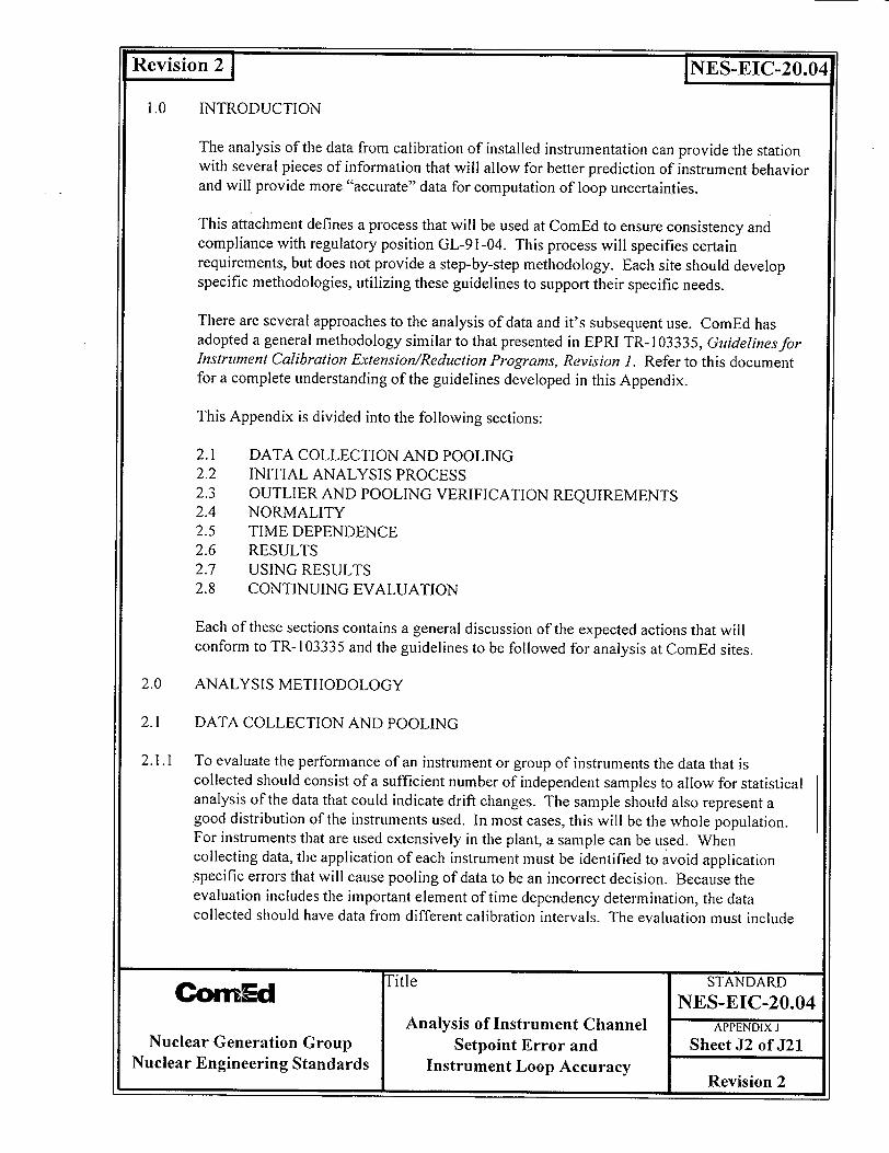
Revision 2 1 INES-EIC-20.04
1.0 INTRODUCTION
The analysis of the data from calibration of installed instrumentation can provide the station with several pieces of information that will allow for better prediction of instrument behavior and will provide more "accurate" data for computation of loop uncertainties.
This attachment defines a process that will be used at CoinEd to ensure consistency and compliance with regulatory position GL-91-04. This process will specifies certain requirements, but does not provide a step-by-step methodology. Each site should develop specific methodologies, utilizing these guidelines to support their specific needs.
There are several approaches to the analysis of data and it's subsequent use. ComEd has adopted a general methodology similar to that presented in EPRI TR-103335, Guidelines for Instrument Calibration Extension/Reduction Programs, Revision ]. Refer to this document for a complete understanding of the guidelines developed in this Appendix.
This Appendix is divided into the following sections:
2.1 DATA COLLECTION AND POOLING 2.2 INITIAL ANALYSIS PROCESS 2.3 OUTLIER AND POOLING VERIFICATION REQUIREMENTS 2.4 NORMALITY 2.5 TIME DEPENDENCE 2.6 RESULTS 2.7 USING RESULTS 2.8 CONTINUING EVALUATION
Each of these sections contains a general discussion of the expected actions that will conform to TR-103335 and the guidelines to be followed for analysis at CoinEd sites.
2.0 ANALYSIS METHODOLOGY
2.1 DATA COLLECTION AND POOLING
2.1.1 To evaluate the performance of an instrument or group of instruments the data that is collected should consist of a sufficient number of independent samples to allow for statistical analysis of the data that could indicate drift changes. The sample should also represent a good distribution of the instruments used. In most cases, this will be the whole population. For instruments that are used extensively in the plant, a sample can be used. When collecting data, the application of each instrument must be identified to avoid application specific errors that will cause pooling of data to be an incorrect decision. Because the evaluation includes the important element of time dependency determination, the data collected should have data from different calibration intervals. The evaluation must include
ow -0 Title STANDARD cbrn~d NES-EIC-20.04
Analysis of Instrument Channel APPENDIX J Nuclear Generation Group Setpoint Error and Sheet J2 of J21
Nuclear Engineering Standards Instrument Loop Accuracy Revision 2

Revision 2 1 INES-EIC-20.04
all of the times that the instrument has been calibrated, or checked for accuracy (i.e. surveillance testing without adjustment).
2.1.2 Selection of the Instruments to be Evaluated (Pooled) for a Given Drift Study
2.1.2.1. All instruments evaluated shall be from the same manufacturer and shall perform in an identical manner for the critical parameters that are to be analyzed. Determining which instruments meet this criterion is eschewed by the fact that many manufacturers' have different model numbers based on mounting, enclosure, etc. The differences typically have no effect on the method that the instrument uses to monitor the parameter of concern. In addition, the range of the instrument may vary without having any significant change in the measurement method. If multiple model numbers are used, the evaluations must include a discussion of the reason why the instruments are assumed identical, specifically in the critical areas of concern.
2.1.2.2. CoinEd has specified that the minimum targeted number of valid data points that are required to make a drift study statistically significant shall be 30 data points. The sample value of 30 is generally accepted as a minimum valid sample size. An analysis using less than this number can be performed ifjustification is provided in the study results. To allow for the potential of an outlier, this number should be > 30 data points. If there are more than approximately 150 data points, there is no significant improvement in the statistical rigor of the analysis.
2.1.2.3. In order to obtain the necessary number of data points required to ensure that there is variance in the calibration interval for the make/model of concern, the calibration data from multiple instruments will be needed. The following criteria for the selection of which instruments and calibration data points shall be used:
a. All instruments that are directly associated with RPS/ESF/ECCS automatic trips and actuations shall include at least one channel's instruments.
b. To ensure that there is a historical perspective to the data evaluated, at least four calibration intervals of data shall be collected. The four intervals provide for historical data while ensuring that the more recent calibration data is used to detect current problems. If the instrument has not been installed for that period, then the available data will be used. There may be some problems in the evaluation of the instrument over a given calibration interval.
c. If more than 150 data points can be developed for a given analysis, then a sample of instruments can be used instead of the whole population. The selection of which instruments to include will be done on a random basis, provided Section 2.1.2.3.a requirements are maintained. The method of selection will be prepared and included in the calculation.
Title STANDARD ConEd NES-EIC-20.04 Analysis of Instrument Channel APPENDIX J
Nuclear Generation Group Setpoint Error and Sheet J3 of J21 Nuclear Engineering Standards Instrument Loop Accuracy Revision 2

Revision 2 1 INES-EIC-20.04
2.1.3 Data Collection is the transfer of data from the calibration records to the final analysis tool. This is a very sensitive process that will require independent verification and validation of data transferred.
2.1.3.1 A search of all preventive and corrective maintenance records shall be conducted on each instrument selected for inclusion in the study. This search shall identify every calibration and every corrective maintenance activity for the period of concern for the study. The search should go back at least four calibration intervals (i.e. at least five sets of calibration data). If there are less than eight instruments included in the study then additional historical data will need to be collected to achieve the minimum number of data points specified by Section 2.1.2.2.
The data collected should ensure that the results are not from overlapping calibration intervals.
2.1.3.2 The data from the calibrations will be entered into a spreadsheet or data base program using a format similar to Figure J1. For instruments that have multiple calibration points (transmitters, function generators, etc.) each calibration point will be entered in the spreadsheet using the percent of span as the column title. If there are discrepancies in the exact percent of span then calibration points that are within 5% of each other can be used together (e.g. 0% FS, 1% FS and 5% FS can be considered the same calibration point).
For switches, relays or other equipment where there is a single point that is calibrated the data can be entered in percent of instrument span or in process units.
Due to the diversity of software that can be used to compute this spreadsheet statistics, there may be some variation in format. The specific project or calculation shall identify the software used and justify that the data entry is in agreement with the intent of Section 4.0 of TR-103335.
"Title STANDARD COrn=d NES-EIC-20.04
Analysis of Instrument Channel APPENDIX J Nuclear Generation Group Setpoint Error and Sheet J4 of J21
Nuclear Engineering Standards Instrument Loop Accuracy I ?ý I [ Revision 2

Revision 2 j-�|I
Figure J1, Example Spreadsheet Data Entry
The following information is particularly valuable for the analysis:
* The date of calibration is documented. The time interval since the previous calibration is calculated in months in the Interval column. Depending on the data, the time interval might be calculated in days, weeks, or months.
* The as-found and as-left data are entered into the spreadsheet exactly as recorded on the instrument data sheet. The values are in milliamperes (in this case) corresponding to a range of 0% to 100% of calibrated span.
• Note that all calibration data points have been recorded. In general, it is preferable to consider and evaluate all available data. By this approach, a better understanding of instrument drift can be obtained.
For calibrations that check calibration points during ascending and descending calibration, the ascending and descending point will be kept separately for the initial evaluation.
Title STANDARD CbrnEd NES-EIC-20.04 Analysis of Instrument Channel APPENDIX J
Nuclear Generation Group Setpoint Error and Sheet J5 of J21 Nuclear Engineering Standards Instrument Loop Accuracy In I I Revision 2
Initial Data AnalysisDate Data Interval Tag Calibration Data (mA)
Mo. Yr. Status Months Number 0% 25% 50% 75% .100%
5 93 As- 12 LT-459 4.00 8.00 11.94 15.96 20.01 Found
As-Left LT-459 4.00 8.00 11.94 15.96 20.01 5 92 As- 14 LT-459 4.20 8.04 12.05 16.05 20.04
Found As-Left LT-459 4.00 8.00 11.98 15.98 20.00
3 91 As- 11 LT-459 4.09 8.04 12.02 16.05 20.04 Found As-Left LT-459 4.09 8.04 12.02 16.05 20.04
4 90 As- 10 LT-459 4.06 7.92 11.95 15.98 19.95 Found As-Left LT-459 4.06 7.92 11.95 15.98 19.95
6 89 As- 13 LT-459 4.00 8.00 12.02 16.07 20.02 Found
As-Left LT-459 4.00 8.00 12.02 16.07 20.02 5 88 As- 12 LT-459 4.24 8.20 12.16 16.12 20.15
Found As-Left LT-459 4.00 7.97 11.98 15.98 20.00
5 87 As- LT-459 NEW NEW NEW NEW NEW Found
As-Left LT-459 4.02 7.99 11.99 16.07 20.01
INES-EIC-20.041

Revision 2 1 INES-EIC-20.04
2.1.3.3 All Data transfer will require 100% independent verification.
2.1.3.4. Due to legibility problems, even if it is obvious that the data recorded in original records is incorrect, verbatim transcription of the data is required. If the information cannot be determined from the original record (due to legibility problems) then the data point will be left blank. Record of this omission shall be included in the analysis.
2.1.3.5 In addition to the calibration point as-found and as-left values, the calibrated span of the instrument, date of the calibration and any significant calibration anomalies are to be recorded in the spreadsheet.
2.2 INITIAL ANALYSIS PROCESS
2.2.1 From the original data, certain manipulations may be required to get the data in a form that can be evaluated across various instruments.
2.2.1.1 If the instrument loop is not a linear loop and the data has not been converted, then the raw calibration data should be converted to Linear Equivalent Full Scale (LEFS) to ensure that drift information is not masked.
2.2.1.2 If the instrument has a known span, the data should be normally converted into percent of calibrated span by dividing the raw data by the span.
If the instrument does not have a known span, the data should be left in process units or converted to percent of the setpoint.
2.2.1.3 For each calibration interval where there is an as-left value from the older calibration and an as-found value from the younger calibration, a raw drift value should be determined by subtracting the as-left value from the as-found value. The calibration interval, in days, should also be determined.
2.2.2 Once the data is in the correct format, the number of data points, the average and the sample standard deviation should be determined for each column, (reference Section 4.0 of TR103335).
Due to the diversity of software that can be used to compute this spreadsheet statistics, there may be some variation in format. The specific project or calculation should identify the software used and justify that the data entry is in agreement with this Standard.
2.3. OUTLIER AND POOLING VERIFICATION REQUIREMENTS
Title STANDARD
COwnEd NES-EIC-20.04 Analysis of Instrument Channel APPENDIX J
Nuclear Generation Group Setpoint Error and Sheet J6 of J21 Nuclear Engineering Standards Instrument Loop Accuracy Revision 2
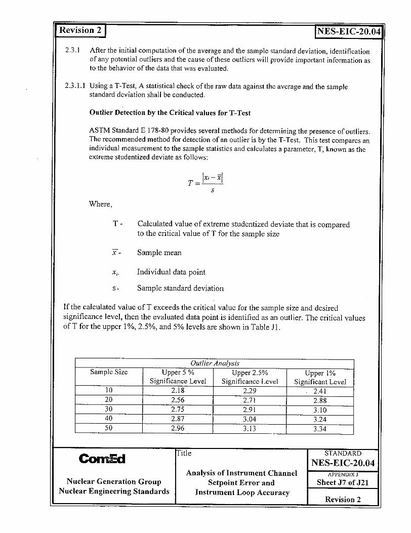
Revision 2 J INES-EIC-20.042.3.1 After the initial computation of the average and the sample standard deviation, identification
of any potential outliers and the cause of these outliers will provide important information as to the behavior of the data that was evaluated.
2.3.1.1 Using a T-Test, A statistical check of the raw data against the average and the sample standard deviation shall be conducted.
Outlier Detection by the Critical values for T-Test
ASTM Standard E 178-80 provides several methods for determining the presence of outliers. The recommended method for detection of an outlier is by the T-Test. This test compares an individual measurement to the sample statistics and calculates a parameter, T, known as the extreme studentized deviate as follows:
T - xi -Y
Where,
T - Calculated value of extreme studentized deviate that is compared to the critical value of T for the sample size
x- Sample mean
xi_ Individual data point
s- Sample standard deviation
If the calculated value of T exceeds the critical value for the sample size and desired significance level, then the evaluated data point is identified as an outlier. The critical values of T for the upper 1%, 2.5%, and 5% levels are shown in Table J1.
P-d ritle STANDARD
COrnCd NES-EIC-20.04 Analysis of Instrument Channel APPENDIX J
Nuclear Generation Group Setpoint Error and Sheet J7 of J21 Nuclear Engineering Standards Instrument Loop Accuracy Revision 2
Outlier Analysis Sample Size Upper 5 % Upper 2.5% Upper 1%
Significance Level Significance Level Significant Level 10 2.18 2.29 2.41 20 2.56 2.71 2.88 30 2.75 2.91 3.10 40 2.87 3.04 3.24 50 2.96 3.13 3.34
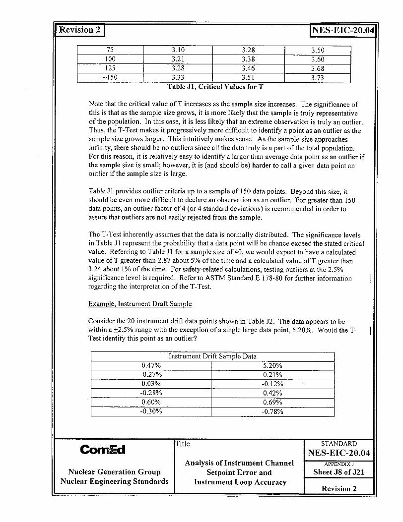
oI 0
75 3.10 3.28 3.50 100 3.21 3.38 3.60 125 3.28 3.46 3.68
-150 3.33 3.51 3.73 Table J1, Critical Values for T
Note that the critical value of T increases as the sample size increases. The significance of this is that as the sample size grows, it is more likely that the sample is truly representative of the population. In this case, it is less likely that an extreme observation is truly an outlier. Thus, the T-Test makes it progressively more difficult to identify a point as an outlier as the sample size grows larger. This intuitively makes sense. As the sample size approaches infinity, there should be no outliers since all the data truly is a part of the total population. For this reason, it is relatively easy to identify a larger than average data point as an outlier if the sample size is small; however, it is (and should be) harder to call a given data point an outlier if the sample size is large.
Table J1 provides outlier criteria up to a sample of 150 data points. Beyond this size, it should be even more difficult to declare an observation as an outlier. For greater than 150 data points, an outlier factor of 4 (or 4 standard deviations) is recommended in order to assure that outliers are not easily rejected from the sample.
The T-Test inherently assumes that the data is normally distributed. The significance levels in Table J 1 represent the probability that a data point will be chance exceed the stated critical value. Referring to Table J1 for a sample size of 40, we would expect to have a calculated value of T greater than 2.87 about 5% of the time and a calculated value of T greater than 3.24 about 1% of the time. For safety-related calculations, testing outliers at the 2.5% significance level is required. Refer to ASTM Standard E 178-80 for further information regarding the interpretation of the T-Test.
Example, Instrument Draft Sample
Consider the 20 instrument drift data points shown in Table J2. The data appears to be within a +2.5% range with the exception of a single large data point, 5.20%. Would the TTest identify this point as an outlier?
Instrument Drift Sample Data 0.47% 5.20% -0.27% 0.21% 0.03% -0.12% -0.28% 0.42% 0.60% 0.69% -0.30% -0.78%
Title STANDARD COrEd NES-EIC-20.04
Analysis of Instrument Channel APPENDIX J
Nuclear Generation Group Setpoint Error and Sheet J8 of J21 Nuclear Engineering Standards Instrument Loop Accuracy Revision 2
Revision 2 1 INES-EIC-20.041
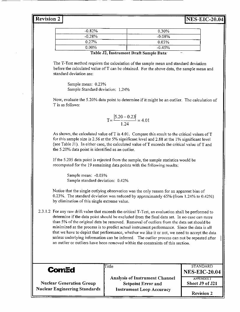
U-
Revision2 INES-EIC-20.04
-0.82% 0.30% -0.28% -0.08% 0.27% 0.03% 0.00% -0.45%
Table J2, Instrument Draft Sample Data-
The T-Test method requires the calculation of the sample mean and standard deviation before the calculated value of T can be obtained. For the above data, the sample mean and standard deviation are:
Sample mean: 0.23% Sample Standard deviation: 1.24%
Now, evaluate the 5.20% data point to determine if it might be an outlier. The calculation of T is as follows:
T= 15.20 - 0.231 = 4.01 1.24
As shown, the calculated value of T is 4.01. Compare this result to the critical values of T for this sample size is 2.56 at the 5% significant level and 2.88 at the 1% significant level (see Table Jl). In either case, the calculated value of T exceeds the critical value of T and the 5.20% data point is identified as an outlier.
If the 5.205 data point is rejected from the sample, the sample statistics would be recomputed for the 19 remaining data points with the following results:
Sample mean: -0.03% Sample standard deviation: 0.42%
Notice that the single outlying observation was the only reason for an apparent bias of 0.23%. The standard deviation was reduced by approximately 65% (from 1.24% to 0.42%) by elimination of this single extreme value.
2.3.1.2 For any raw drift value that exceeds the critical T-Test, an evaluation shall be performed to determine if the data point should be excluded from the final data set. In no case can more than 5% of the original data be removed. Removal of outliers from the data set should be minimized as the process is to predict actual instrument performance. Since the data is all that we have to depict that performance, whether we like it or not, we need to accept the data unless underlying information can be inferred. The outlier process can not be repeated after an outlier or outliers have been removed within the constraints of this section.
STitle STANDARD COrnEd NES-EIC-20.04
Analysis of Instrument Channel APPENDIX J Nuclear Generation Group Setpoint Error and Sheet J9 of J21
Nuclear Engineering Standards Instrument Loop Accuracy Revision 2
Revision 2 1 INES-EIC-20.04
2.3.1.3 Identification of a potential outlier in Section 2.3.1.2 does not mean that the value will be automatically excluded. Examples of when outliers should be removed include:
a. Review of the calibration indicates that a data entry error was likely. This will normally be seen as a random value that is significantly.outside the rest of the data with no explanation. This type of outlier is a rare event and should not be done routinely.
b. Review of the data indicates that a bad calibration was performed. This will normally be seen by multiple outliers from the same calibration and a reverse drift of similar magnitude in the next calibration. In these cases, both sets of raw data should be removed.
2.3.1.4 The pattern of outliers should also be evaluated to determine if there is a bad instrument or application that is contaminating the data set.
It is permissible for this evaluation to rerun the T-Test with a smaller critical T value to force outliers. If this is done, these outliers should not be removed from the final data set.
This process will provide a number of data points that were at the extremes of the data set. If these extremes were primarily in one instruments' data or in one application area then additional evaluations need to be performed to determine if this data can be used with the rest of the data..
2.3.1.5 Bad instruments or bad applications will be detectable from the outliers that are identified. The best indication will be that the outliers will be bunched in the instrument or instruments used for a specific application. Other potential causes that could be identified by this process are:
a. Variations in range or span b. Variations in age of calibration or equipment.
2.3.1.6 If the result of the outlier analysis indicates the potential for an application, range, age, etc. type of problem, then an analysis of the selection at that particular instrument should be conducted. Inclusion of data from any instrument can be checked by comparing this mean and variance of the instrument data to the mean and variance to the remainder of the data as explained in TR-103335 Section B.9.
2.4 NORMALITY
2.4.1 *For this analysis, the assumption of normality is an integral assumption. To ensure that the data is a normal distribution or that a normal distribution is a conservative assumption, a test
"M -K Title STANDARD DOmn= NES-EIC-20.04 Analysis of Instrument Channel APPENDIX J
Nuclear Generation Group Setpoint Error and Sheet J10 of J21 Nuclear Engineering Standards Instrument Loop Accuracy Revision 2
Revision 2 1 INES-EIC-20.04
for normality of the data will be performed for all as-found/as-left data analysis after any outliers have been removed.
2.4.2 There are several tests for the normality of a data set. (See Appendix C of TR-103335). ComEd requires at least one of the following numerical approaches be conducted before the qualitative evaluations are performed.
" Chi-Squared. X2,. Goodness of Fit Test. This well known test is stated as a method for
assessing normality in ISA-RP67.04, Recommended Practice, Methodologies for the Determination of Setpoints for Nuclear Safety-Related Instrumentation.
" WTest. This test is recommended by ANSI N 15.15-1974, Assessment of the Assumption of Normality (Employing Individual Observed Values), for sample sizes less than 50.
" D-Prime Test. This test is recommended by ANSI N15.15-1974, Assessment of the Assumption of Normality (Employing Individual Observed Values), for moderate to large sample sizes.
2.4.3 If normality cannot be determined from a standard test then the data should be evaluated to determine if the assumption of normality is a conservative assumption. This can be done by one of the following techniques:
Probability Plots. Probability plots (See Figure J2) provide a graphical presentation of the data that can reveal possible reasons for why the data is or is not normal. Use of a probability plot and qualitative evaluation demonstrates how close the tails of the curve approach a diagonal.
Title STANDARD COrnEd NES-EIC-20.04
Analysis of Instrument Channel APPENDIX J
Nuclear Generation Group Setpoint Error and Sheet J1l of J21
Nuclear Engineering Standards Instrument Loop Accuracy I I Revision 2
I
I
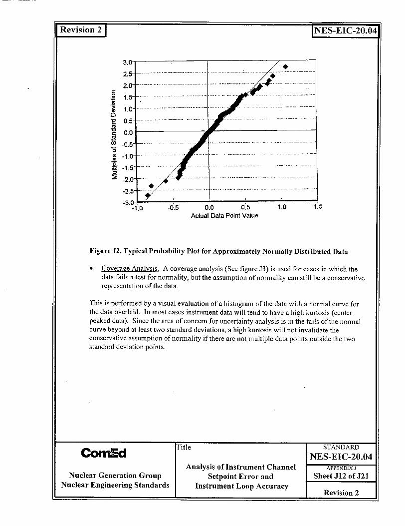
Revision22
2.5-
a
0
70 °n
°0 C~
a,
0
U, "a,
1.5
1.0
0.5
0.0
-0.5
-1.0
-1.5
-2.5
-1.0 -0.5 0.0 0.5Actual Data Point Value
Figure J2, Typical Probability Plot for Approximately Normally Distributed Data
* Coverage Analysis. A coverage analysis (See figure J3) is used for cases in which the data fails a test for normality, but the assumption of normality can still be a conservative representation of the data.
This is performed by a visual evaluation of a histogram of the data with a normal curve for the data overlaid. In most cases instrument data will tend to have a high kurtosis (center peaked data). Since the area of concern for uncertainty analysis is in the tails of the normal curve beyond at least two standard deviations, a high kurtosis will not invalidate the conservative assumption of normality if there are not multiple data points outside the two standard deviation points.
N Title STANDARD COrn d NES-EIC-20.04
Analysis of Instrument Channel APPENDIXJ Nuclear Generation Group Setpoint Error and Sheet J12 of J21
Nuclear Engineering Standards Instrument Loop Accuracy Revision 2
INES-EIC-20.04
a I
1.0 1.5
...• ....... ...... i........... . !!i!i-i

Revision 2 1
300
250
200-(D 07 150
LI.
100
50
0
INES-EIC-20.04
Figure J3, Coverage Analysis Histogram
2.4.4 If normality or a bounding condition of normality cannot be assumed for the data set, then depending on the distribution:
a. b.
A distribution free tolerance value must be determined. The size of the standard deviation will be expanded to bound the distribution.
As this is a seldom used case, this will not be discussed in this Standard. Refer to standard statistics texts for binomial and distribution free statistical method.
To determine the amount of increase needed from the tabular 95/95 value for the histogram evaluation, use the count in each bar of the histogram and ensure that greater than 95% of the data is captured. Increase the standard deviation as necessary to capture at least 95% of the data.
2.5 TIME DEPENDENCE
2.5.1 The way the resultant drift value from this as-found/as-left analysis is used is very sensitive to the determination of the time dependency.
This is particularly important for the extension of operating cycles via the NRC Generic Letter 91-04. This drift analysis requires that some decision be made on how the drift at thirty months can be determined from data that is taken over an eighteen month period.
2.5.2 The basic assumption that drift is linear time dependant will be used for the initial evaluation of the computed drift.
Title STANDARD CbnmEd NES-EIC-20.04
Analysis of Instrument Channel APPENDIX J Nuclear Generation Group Setpoint Error and Sheet J13 of J21
Nuclear Engineering Standards Instrument Loop Accuracy Revision 2
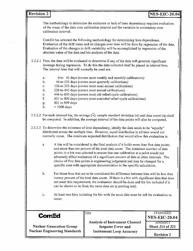
Revision 2 1 INES-EIC-20.04
The methodology to determine the existence or lack of time dependency requires evaluation of the mean of the data over calibration interval and the variation in uncertainty over calibration interval.
ComEd has selected the following methodology for determining time dependence. Evaluation of the drift mean and its changes over time will be done by regression of the data. Evaluation of the changes in drift variability will be accomplished by regression of the absolute value of the data and bin analysis of the data.
2.5.2.1 First, the data will be evaluated to determine if any of the data will generate significant leverage during regression. To do this the data collected shall be placed in interval bins. The interval bins that will normally be used are:
a. 0 to 45 days (covers most weekly and monthly calibrations) b. 46 to 135 days (covers most quarterly calibrations) c. 136 to 225 days (covers most semi-annual calibrations) d. 226 to 445 days (covers most annual calibrations) e. 446 to 650 days (covers most old refuel cycle calibrations) f. 651 to 800 days (covers most extended refuel cycle calibrations) g, 801 to 999 days h. > 1000 days
2.5.2.2 For each internal bin, the average (x), sample standard deviation (a) and data count (rq) shall be computed. In addition, the average interval of the data points will also be computed.
2.5.2.3 To determine the existence of time dependency, ideally the data needs to be "equally" distributed across the multiple bins. However, equal distribution in all bins would not normally occur. The minimum expected distribution that would allow this evaluation is:
a. A bin will be considered in the final analysis if it holds more than five data points and more than ten percent of the total data count. The minimum number of data points in a bin was selected to ensure that one calibration at a point would not adversely affect evaluation of a significant amount of data at other intervals. The choice of five data points is engineering judgement and may be changed for a specific case with appropriate documentation in the specific calculation.
b. For those bins that are to be considered the difference between bins will be less than twenty percent of the total data count. If there is a bin with significant data that does not meet this requirement, the evaluation should be done and the bin included if it can be shown to be from the same data set (a pooling test).
c. At least two bins including the bin with the most data must be left for evaluation to Occur.
Title STANDARD ComnEd NES-EIC-20.04 Analysis of Instrument Channel APPENDIX J
Nuclear Generation Group Setpoint Error and Sheet J14 of J21 Nuclear Engineering Standards Instrument Loop Accuracy
I I I Revision 2

Revision 2 J
The following example demonstrates the process described above.
INES-EIC-20.04
itle STANDARD CtrnEd NES-EIC-20.04
Analysis of Instrument Channel APPENDIX J Nuclear Generation Group Setpoint Error and Sheet J15 of J21
Nuclear Engineering Standards Instrument Loop Accuracy Revision 2
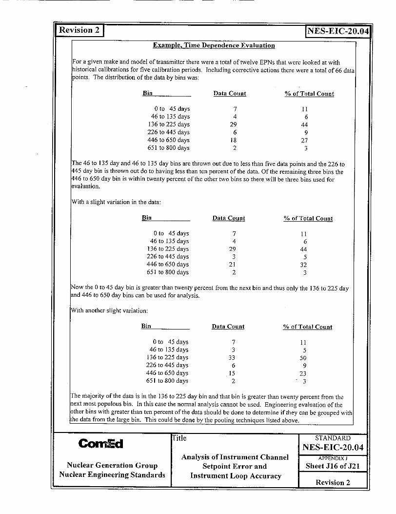
Revision 2 [NES-EIC-20.04
Example, Time Dependence Evaluation
For a given make and model of transmitter there were a total of twelve EPNs that were looked at with historical calibrations for five calibration periods. Including corrective actions there were a total of 66 data points. The distribution of the data by bins was:
Bin Data Count % of Total Count
0to 45 days 7 11 46 to 135 days 4 6
136 to 225 days 29 44 226 to 445 days 6 9 446 to 650 days 18 27 651 to 800 days 2 3
The 46 to 135 day and 46 to 135 day bins are thrown out due to less than five data points and the 226 to 445 day bin is thrown out do to having less than ten percent of the data. Of the remaining three bins the 446 to 650 day bin is within twenty percent of the other two bins so there will be three bins used for evaluation.
With a slight variation in the data:
Bin Data Count % of Total Count
0to 45 days 7 11 46 to 135 days 4 6
136 to 225 days 29 44 226 to 445 days 3 5 446 to 650 days 21 32 651 to 800 days 2 3
Now the 0 to 45 day bin is greater than twenty percent from the next bin and thus only the 136 to 225 day and 446 to 650 day bins can be used for analysis.
With another slight variation:
Bin Data Count % of Total Count
0to 45 days 7 11 46 to 135 days 3 5
136 to 225 days 33 50 226 to 445 days 6 9 446 to 650 days 15 23 651 to 800 days 2 3
The majority of the data is in the 136 to 225 day bin and that bin is greater than twenty percent from the next most populous bin. In this case the normal analysis cannot be used. Engineering evaluation of the other bins with greater than ten percent of the data should be done to determine if they can be grouped with the data from the large bin. This could be done by the pooling techniques listed above.
Title STANDARD COrnEd NES-EIC-20.04
Analysis of Instrument Channel APPENDIX J Nuclear Generation Group Setpoint Error and Sheet J16 of J21
Nuclear Engineering Standards Instrument Loop Accuracy Revision 2
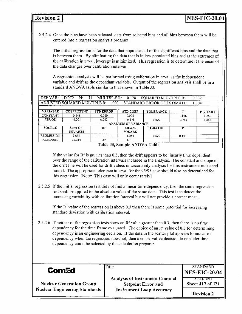
Revision 2 1 NES-EIC-20.04
2.5.2.4 Once the bins have been selected, data from selected bins and all bins between them will be entered into a regression analysis program.
The initial regression is for the data that populates all of the significant bins and the data that is between them. By eliminating the data that is in low populated bins and at the extremes of the calibration interval, leverage is minimized. This regression is to determine if the mean of the data changes over calibration interval.
A regression analysis will be performed using calibration interval as the independent variable and drift as the dependant variable. Output of the regression analysis shall be in a standard ANOVA table similar to that shown in Table J3.
DEP VAR: DOT2 N: 31 MULTIPLE R: 0.178 SQUARED MULTIPLE R: 0.032 ADJUSTED SQUARED MULTIPLE R: .000 STANDARD ERROR OF ESTIMATE: 1.304
VARIABLE COEFFICIENT STD ERROR STD COEF TOLERANCE T P (2 TAIL) CONSTANT 0.848 0.740 0.000 1.146 0.266
PERIOD -0.001 0.002 -0.178 1.000 -0.787 0.44 t ANALYSIS OF VARIANCE
SOURCE SUM-OF- DF MEAN- F-RATIO SQUARES SQUARE
REGRESSION 1.054 1 1.054 0.620 0.441 RESIDUAL 32.319 29 1.701
Table J3, Sample ANOVA Table
If the value for R2 is greater than 0.3, then the drift appears to be linearly time dependent over the range of the calibration intervals included in the analysis. The constant and slope of the drift line will be used for drift values in uncertainty analysis for this instrument make and model. The appropriate tolerance interval for the 95/95 case should also be determined for this regression. [Note: This case will only occur rarely]
2.5.2.5 If the initial regression test did not find a linear time dependency, then the same regression test shall be applied to the absolute value of the same data. This test is to detect the increasing variability with calibration interval but will not provide a correct mean.
If the R2 value of the regression is above 0.3 then there is some potential for increasing standard deviation with calibration interval.
2.5.2.6 If neither of the regression tests show an R2 value greater than 0.3, then there is no time dependency for the time frame evaluated. The choice of an R2 value of 0.3 for determining dependency is an engineering decision. If the data in the scatter plot appears to indicate a dependency when the regression does not, then a conservative decision to consider time dependency could be selected by the calculation preparer.
Title STANDARD CO nEd NES-EIC-20.04
Analysis of Instrument Channel APPENDIX J Nuclear Generation Group Setpoint Error and Sheet J17 of J21
Nuclear Engineering Standards Instrument Loop Accuracy Revision 2
Revision 2 1 INES-EIC-20.04
2.5.2.7 For those cases with no apparent time dependency, one additional check should be performed to identify any potential problems resulting from increasing uncertainty.
The evaluation of the mean and standard deviation of each bin of significance will provide visual trending of the mean and standard deviation with calibration interval.
For each bin that was evaluated, plot the mean and sample standard deviation against the average calibration interval for that bin. These plots will provide visual indication of the stability of the mean and sample standard deviation for the data available. Indications of increased magnitude of the mean and/or the standard deviation with increasing or decreasing calibration interval can be qualitatively assessed.
A linear extrapolation of the expected increase in sample standard deviation and mean to the next bin outside the analyzed interval can be determined through the regression of the plotted values for the mean and standard deviation. This will provide a value for the mean and sample standard deviation, in Units/Day, for projection into the next bin.
2.5.3 If two or more bins were not identified for analysis then the value of drift from this evaluation must determined from the data from the most populated bin. For this case the process utilized is:
2.5.3.1 Compute the mean and sample standard deviation for the most populated bin. In addition, compute the average calibration interval for the data in that bin.
2.5.3.2 Compute the bias (Section 2.6.1.1) and the tolerance (Section 2.6.1.3). The tolerance value is assumed to be random, allowing the use of the Square Root Sum of the sum of the Squares combination for longer time intervals.
2.5.3.3 Define the drift as either:
a. Time dependent with a bias and tolerance for the period up to the average calibration interval of the bin.
b. Time independent using the 99/95 tolerance value. Historically as-found/as-left studies have not identified any time dependency in drift. By using this expanded tolerance interval this historical information will allow expansion of time independent drift to one bin either side of the bin used for the analysis.
2.6 RESULTS
Title STANDARD COwnEd NES-EIC-20.04
Analysis of Instrument Channel APPENDIX J Nuclear Generation Group Setpoint Error and Sheet J18 of J21
Nuclear Engineering Standards Instrument Loop Accuracy Revision 2

Revision 2 [NES-EIC-20.04
2.6.1 The results of these as-found/as-left analyses determine a value of derived drift for the instrument make/model will be determined. This value will require the following minimum elements:
2.6.1.1 Bias - Will normally be either the mean of the final data set for time independent drift or the intercept (constant) and slope for linear time dependent drift. For time dependent drift, this cannot be from the regression of the absolute value data set but from the final data set. A mean that is less than 0.1% FS will be assumed to be zero. This is a standard value. Bias below this value has no significant effect on the loop uncertainty.
2.6.1.2 Time Dependent Drift Value - For drift that was classified as time dependent, the slope of the regression curve (Units/Day) is the dependent drift value. If this number was determined from the absolute value regression, it still should be specified.
2.6.1.3 Tolerance Value - This value will come from the regression study for time dependent drift. For time independent drift, it will be the sample standard deviation times a multiplier based on the sample size. The selection of the multiplier will be based on the required expectations. Some specific requirements are:
99/95 - For cases where only one bin has sufficient data for analysis use this tolerance if the intent is to still assume time independent drift.
95/95 - For RPS and ECCS automatic actuations. If any instruments of the make/model are used for this then the result must be this confidence and tolerance interval.
95/75 - For other safety related instrumentation. If no instruments of this make/model are used for automatic actuations but they are used in safety related indication and alarm circuits then the tolerance value can be reduced to 75%.
75/75 - If the make/model is only used for non-safety related activities.
2.6.1.4 Valid Interval -The bounds of the calibration interval that were included in the analysis. For the above example, the first case would be 0 to 650 days and the second case would be 136 to 650 days. As extrapolation of statistical evaluations are not normally done this provides the data over the range where it should be valid. Some evaluation of the data within the bounding bins may be necessary to ensure that all of the data is not bunched at one interval. If there is bunching of data, the valid interval should be adjusted to account for this effect.
2.6.1.5 Extrapolation Margin - If the data from the analysis is to be extrapolated to either of the adjacent bins from the Valid Interval, then an additional margin will be added to the results of the evaluation. This additional margin will be:
Title STANDARD
CwrnEd NES-EIC-20.04
Analysis of Instrument Channel APPENDIX J Nuclear Generation Group Setpoint Error and Sheet J19 of J21
Nuclear Engineering Standards Instrument Loop Accuracy ____ ___ ___ ____ ___ ___ ____ ___ ___ ____ ___ ___ ____ ___ ___Revision 2

Revision 2 1 [NES-EIC-20.04
a. Using the value for the mean and standard deviation (Units/Day) from the process described in Section 2.5.2.7, multiply each value by the number of days that the extrapolation is required. The extrapolation cannot go beyond the next bin. All negative values for standard deviation will be set to zero.
b. Add the extrapolated value to the mean and sample standard deviation to obtain an adjusted mean and sample standard deviation. These adjusted values will be the values used for computing the results required in Sections 2.6.1.1, 2.6.1.2 and 2.6.1.3.
2.6.2 The analysis should clearly indicate the make/model that it was performed for, and any functions excluded.
2.7 USING THE RESULTS
2.7.1 The data reduction has generated a "drift" value, but that number includes several uncertainties in addition to the classical drift. If the determined drift value is used in uncertainty calculations, the following uncertainties can normally be eliminated. To replace these values state that they are included in the calculated drift value and set their individual values to zero.
2.7.1.1 Reference Accuracy - The reference accuracy of the instrument is included in the calibration data and can be removed from the uncertainty calculation.
2.7.1.2 M&TE - As long as the calibration process uses the same, or more accurate, test equipment then this uncertainty is included in the calibration data and can be removed from the uncertainty calculation.
2.7.1.3 Drift - The true drift is included in the determined drift and is included in the calibration data and can be removed from the uncertainty calculation.
2.7.1.4 Normal Environmental Effects - For the instruments that are included in the calibration, the effects of variations in radiation, humidity, temperature, vibration, etc. experienced during the calibration are included in the calibration data and can be removed from the uncertainty calculation. These terms cannot be removed from the uncertainty calculations if these components see different conditions or magnitudes of the parameter, such as vibration or temperature, while operating then during calibration.
2.7.1.5 Power Supply Effects - If the instruments are attached to the same power supply during calibration that is used during operation, then the affects are included in the calibration data and can be removed from the uncertainty calculation.
Title STANDARD OrnEd NES-EIC-20.04
Analysis of Instrument Channel APPENDIX J Nuclear Generation Group Setpoint Error and Sheet J20 of J21
Nuclear Engineering Standards Instrument Loop Accuracy Revision 2
Revision 2 INES-EIC-20.04
2.7.2 For cases were there are time dependent drifts, the time frame used for determining the drift should be the normal surveillance interval plus twenty-five percent.
Time dependent drift that is random is assumed to be normally distributed and can be combined using the Square Root Sum of the Squares method for-intervals beyond the given interval for the drift as explained in Appendix A and C to this procedure.
2.7.3 Time independent drift can be assumed to be constant over the Valid Interval. It can also be assumed constant over the interval in the next bin if the Extrapolation Margin is applied.
2.8 CONTINUING EVALUATION
2.8.1 To maintain these evaluations current and to detect increasing drift, the process stipulated in CC-AA-520 "Instrument Performance Trending" shall be followed.
Title STANDARD GOw Ed NES-EIC-20.04
Analysis of Instrument Channel APPENDIX J
Nuclear Generation Group Setpoint Error and Sheet J21 of J21 Nuclear Engineering Standards Instrument Loop Accuracy Revision 2

ATTACHMENT 2
Commonwealth Edison Company Letter, "Supplemental Information to Support Request for Technical Specifications Changes," dated June 5, 2000
Dresden Nuclear Power Station, Units 2 and 3 LaSalle County Station, Units 1 and 2
Quad Cities Nuclear Power Station, Units 1 and 2
Justification for 24-Month Surveillance Requirement Frequencies

Justification for 24-Month Surveillance Requirement Frequencies
PURPOSE:
To accommodate a 24-month fuel cycle for Dresden Nuclear Power Station, Units 2 and 3, LaSalle County Station, Units 1 and 2, and Quad Cities Nuclear Power Station, Units 1 and 2, Commonwealth Edison (ComEd) is integrating the necessary changes to the Dresden Nuclear Power Station, Units 2 and 3, LaSalle County Station, Units 1 and 2, and Quad Cities Nuclear Power Station, Units 1 and 2, Technical Specifications Surveillance Requirements into the documents being used to convert to the Improved Standard Technical Specifications. To facilitate the review of the 24-month fuel cycle portion of this submittal, the following overview document is being provided to identify the scope of changes and the methodology used to justify the changes.
It is intended to implement longer fuel cycles for Dresden Nuclear Power Station, Units 2 and 3, LaSalle County Station, Units 1 and 2, and Quad Cities Nuclear Power Station, Units 1 and 2, during the current operating cycles. The proposed changes are submitted in support of the 24-month fuel cycle conversion. As demonstrated in this submittal, the proposed changes will not adversely impact safety. The proposed changes are being submitted to the NRC as a Cost Beneficial Licensing Action, and are similar to license amendments issued for a number of other nuclear units.
The proposed changes were evaluated in accordance with the guidance provided in NRC Generic Letter 91-04, "Changes in Technical Specification Surveillance Intervals to Accommodate a 24 Month Fuel Cycle," dated April 2, 1991.
Historical surveillance test data and associated maintenance records were reviewed in evaluating the effect on safety. In addition, the licensing basis was reviewed for each revision to ensure it was not invalidated. Based on the results of these reviews, it is concluded that there is no adverse effect on plant safety due to increasing the surveillance test intervals from 18 to 24 months and the continued application of Surveillance Requirement (SR) 3.0.2.
I1. SCOPE
The 24-month fuel cycle portion of this submittal includes a justification, when the SR Frequency is being changed from 18 to 24 months. The justification is limited to those existing Current Technical Specification (CTS) Surveillance Requirements (SRs) that are being retained in the Improved Technical Specifications (ITS) which have a CTS Frequency of 18 months. New SRs for ITS have been evaluated (qualitatively or quantitatively) for a Frequency of 24 months.
These changes have been divided into two categories. The categories are: 1) changes involving the Channel Calibration Frequency identified as "Instrumentation Changes" (identified in the ITS conversion document Discussion of Changes as "LEs"), and 2) other changes identified as "Non-Instrumentation Changes" (identified in the ITS conversion document Discussion of Changes as "LDs").
Page 1 of 27
III METHODOLOGY
In NRC Generic Letter 91-04, the NRC provided generic guidance for evaluating a 24 month surveillance test interval for Technical Specification (TS) SRs. NRC Generic Letter 91-04 specifies the steps for the evaluation needed to justify a 24 month surveillance interval. The following defines each step outlined by the NRC in Generic Letter 91-04 and provides a description of the methodology used by the Dresden Nuclear Power Station, Units 2 and 3, LaSalle County Station, Units 1 and 2, and Quad Cities Nuclear Power Station, Units 1 and 2, personnel to complete the evaluation for each specific CTS SR line item. This methodology is very similar to the methodology used to justify extensions for a 24-month fuel cycle at the Carolina Power & Light Company Brunswick Nuclear Plant. The Brunswick Nuclear Plant methodology was found acceptable by the NRC in the Brunswick Nuclear Plant ITS124 Month extension Safety Evaluation issued on June 5, 1998.
A. Non-Instrumentation changes ("LD" Discussion of Changes):
NRC Generic Letter 91-04 identifies three steps to evaluate Non-Instrumentation changes:
STEP 1:
"...licensees should evaluate the effect on safety of the change in surveillance intervals to accommodate a 24 Month fuel cycle. This evaluation should support a conclusion that the effect on safety is small."
Evaluation
Dresden Nuclear Power Station, Units 2 and 3, LaSalle County Station, Units 1 and 2, and Quad Cities Nuclear Power Station, Units 1 and 2, have individually evaluated each SR being changed with respect to its effect on plant safety. This evaluation provides a justification for each CTS non-instrumentation SR which is being retained in ITS. The evaluation is summarized in the Discussion of Change identified as "LDs". The following information provides a description of the purpose of surveillance testing and a general description of the methodology utilized to justify the conclusion that extending the testing interval has a minimal effect on safety.
The purpose of surveillance testing is to verify through the performance of the specified SRs that the tested TS Function/Feature will perform as assumed in the associated safety analysis or in accordance with the associated Function's design. By periodically testing the TS Function/Feature, the availability of the associated Function/Feature is confirmed. As such, with the extension of the Dresden Nuclear Power Station, Units 2 and 3, LaSalle County Station, Units 1 and 2, and Quad Cities Nuclear Power Station, Units I and 2, operating cycle and the associated extension of the refueling cycle surveillance test interval (i.e., frequency), a longer period of time will exist between performances of a surveillance test. If a failure resulting in the loss of a Safety Function occurs during the operating cycle and that failure would be detected only by the performance of the periodic TS SR, then the increase in the surveillance testing interval would result in a decrease in the associated Function's availability and thus have a
Page 2 of 27
potential impact on safety.
Each associated non-instrumentation SR has been evaluated to demonstrate that the potential impact on availability, if any, is minimal as a result of the change to a 24-month frequency. A program plan was developed that defined the scope of the analysis to be performed (e.g., failure history analysis) and the methods for performing these analyses. The process included: 1) identification of the 18 month surveillances in the CTS, 2) determining the plant tests that verified the operation of the equipment associated with the surveillance, 3) collection of the test history associated with the function, and 4) evaluation of the test history results. The evaluations were based on the fact that either the Function/Feature is tested on a more frequent basis during the operating cycle by other plant programs (e.g., pump flow rate tested quarterly), is designed to be single failure proof, or is highly reliable.
The more frequent testing may include the performance of Channel Checks which verify that the instrument transmitter and indication are functional, and the system parameters (e.g. pump flow, system pressure, etc.) are within expected values. More frequent testing also includes Channel Functional Tests which verify the operation of circuits associated with alarms, interlocks, displays, trip functions, time delays and channel failure trips. Where a Channel Check or Channel Functional Test is not required, normally the circuit is simple and these checks would not provide any additional assurance that the components are functional. In several cases (e.g. switches) the more frequent testing may not verify the operation of the circuits directly associated with the switch, but may verify the operation of other circuits associated with the Function with which the switch is associated. In most cases the same circuit (with the exception of the open loop associated with the switch) is used for manual operation of a pump and for pump automatic start functions. In these cases the Channel Checks and Channel Functional Tests would also test most of the circuit associated with the initiation push button, with the exception of the switch itself and the wire to connect the switch to the circuit.
Additional testing, such as inservice pump or valve testing, will also verify that the power and control circuits associated with the specific TS components, relays and contacts associated with these components are operational. Inservice programs test components based on performance oriented schedules. The requirements of 10 CFR 50.65, "Requirements for monitoring the effectiveness of maintenance at nuclear power plants," (i.e., Maintenance Rule) also support testing based on safety significant components and their unavailability or performance. Decreased component performance requires increased testing. Some system components may not be tested more frequently based on the impact on plant operation (e.g., Emergency Core Cooling System injection valves). However, performance of these components are tracked on the basis of system availability, and increased failures or maintenance will be identified and corrected as a part of the station's maintenance program.
Additionally, as previously stated by the NRC in Reference 8, industry reliability studies for Boiling Water Reactors (BWRs), prepared by the BWR Owners Group in Reference 9, show that the overall safety systems' reliabilities are not dominated by the reliabilities of the logic system, but by that of the mechanical components, (e.g., pumps and valves), which are consequently tested on a more frequent basis, usually by the Inservice Testing Program. Since the probability of a relay or contact failure is small
Page 3 of 27

relative to the probability of mechanical component failure, increasing the logic system functional test interval represents no significant change in the overall safety system unavailability.
STEP 2:
"Licensees should confirm that historical maintenance and surveillance data do not invalidate this conclusion".
EVALUATION
The surveillance test history of the affected SRs has been evaluated. This evaluation consisted of a review of surveillance test results and associated maintenance records. Only SR test failures were evaluated because failures detected by other plant activities such as Preventative Maintenance Tasks or Surveillance Tests that are performed more frequently than 24 months were assumed to continue to detect failures. This review of surveillance test history validated the conclusion that the impact, if any, on system availability will be minimal as a result of the change to a 24 month testing frequency.
STEP 3:
"... licensees should confirm that the performance of surveillances at the bounding surveillance interval limit provided to accommodate a 24-month fuel cycle would not invalidate any assumption in the plant licensing basis."
EVALUATION
As part of the evaluation of each SR, the impact of the changes against the assumptions in the respective Dresden Nuclear Power Station, Units 2 and 3, LaSalle County Station, Units 1 and 2, and Quad Cities Nuclear Power Station, Units 1 and 2, licensing basis was reviewed. In general, these changes have no impact on the plant licensing basis. However, in some cases, the change does require a change to licensing basis information, as described in the Dresden Nuclear Power Station, Units 2 and 3, LaSalle County Station, Units 1 and 2, or Quad Cities Nuclear Power Station, Units 1 and 2, Updated Final Safety Analysis Report (UFSAR). Since no Unreviewed Safety Questions have been identified in the changes, the UFSAR changes will be performed and submitted in accordance with 10 CFR 50.59, "Changes, tests and experiments," and 10 CFR 50.71(e).
The performance of surveillances extended for a 24 month fuel cycle will be trended as a part of the Maintenance Rule Program. Any degradation in performance will be evaluated to verify that the degradation is not due to the extension of surveillance or maintenance activities.
Page 4 of 27
B. Instrumentation (Channel Calibration changes (LE Discussion of Changes)):
NRC Generic Letter 91-04 identifies 7 steps for the evaluation of Instrumentation changes.
STEP 1:
Confirm that instrument drift as determined by as-found and as-left calibration data from surveillance and maintenance records has not, except on rare occasions, exceeded acceptable limits for a calibration interval.
EVALUATION
The effect of longer calibration intervals on the TS instrumentation was evaluated by performing a review of the surveillance test history for the affected instrumentation, including, where necessary, an instrument drift study. In performing the drift study, an effort was made to retrieve recorded Channel Calibration data for associated instruments for the past five operating cycles. By obtaining recorded calibration data for the past several cycles of operation, a true representation of instrument drift can be determined. However, for several different sets of instruments at Dresden Nuclear Power Station, Units 2 and 3, and Quad Cities Nuclear Power Station, Units 1 and 2, sufficient data was not available to perform the drift analysis using data from only one plant. For these cases the data collected from both plants were combined. Generally, the combination of data was limited to identical manufacturer and model numbers performing the same functions in the two plants. In some limited cases, after performing statistical grouping evaluations different model numbers may have also been combined between the plants. The failure history evaluation and drift study demonstrates that except on rare occasions, instrument drift has not exceeded the current allowable limits.
The generic Rosemount failure mode (i.e., calibration failure of Rosemount Transmitters due to loss of fill oil) was identified during 1986 and 1987, based on the failure of five Rosemount model 1153 HD5PC differential pressure transmitters at Northeast Utilities' Millstone Nuclear Power Station, Unit 3. These failures were documented in NRC Information Notice No. 89-42,"Failure of Rosemount Models 1153 and 1154 Transmitters," dated April 21, 1989, and NRC Bulletin No. 90-01, "Loss of Fill-oil in Transmitters Manufactured by Rosemount," dated March 9, 1990. During power operation, the Millstone Nuclear Power Station, Unit 3, operators noted that the signals from the Rosemount 1153 transmitters were deviating from redundant channel signals and that the transmitters were indicating reduced levels of process noise. Further investigation by the NRC and Rosemount lead to identification of the root cause as oil loss from the Rosemount sealed sensing module. NRC Bulletin No. 90-01 and Supplement 1 defined specific replacement and testing criteria for any suspected transmitters. Additionally Supplement 1 to NRC Bulletin No. 90-01 defined a maturity period after which the probability of failure due to oil loss is greatly reduced and monitoring of the transmitters may be performed at longer intervals (not exceeding 24 months).
For the Dresden Nuclear Power Station, Units 2 and 3, and Quad Cities Nuclear Power Station, Units 1 and 2, all applicable Rosemount transmitters have been identified and replaced. For LaSalle County Station, Units 1 and 2, some but not all of the Rosemount
Page 5 of 27
transmitters have been replaced. LaSalle County Station has committed, in response to NRC Bulletin No. 90-01 and Supplement 1, to an enhanced monitoring program for these transmitters. Conflicts between cycle extension and the LaSalle commitment to NRC Bulletin No. 90-01 and Supplement 1 will be addressed separate from the ITS 24month Technical Specification change request.
STEP 2:
Confirm that the values of drift for each instrument type (make, model, and range) and application have been determined with a high probability and a high degree of confidence. Provide a summary of the methodology and assumptions used to determine the rate of instrument drift with time based upon historical plant calibration data.
EVALUATION
Data Collection and Conditioning
Dresden Nuclear Power Station, Units 2 and 3, LaSalle County Station, Units 1 and 2, and Quad Cities Nuclear Power Station, Units 1 and 2, have performed drift evaluations, based on a ComEd Specific Drift Analysis Design Guide (i.e., Appendix J of ComEd Nuclear Engineering Standard NES-EIC-20.04, "Analysis of Instrument Channel Setpoint Error and Instrument Loop Accuracy") provided in Attachment 5. The ComEd Specific Drift Analysis Design Guide is based on EPRI TR-1 03335, "Guidelines for Instrument Calibration Extension/Reduction Programs," Revision 1, dated October 1998. The ComEd methodology utilizes the As Found/As Left (AFAL) analysis methodology to statistically determine drift for current calibration intervals. The AFAL methodology utilizes historical data obtained from surveillance tests. The raw calibration data is conditioned prior to use for the drift calculation. The conditioning consists of eliminating tests or individual data points that do not reflect actual drift. The removed data is limited to data associated or affected by:
a. Instrument failures, b. Procedural problems which affect the calibration data, c. Measurement and Test Equipment (M&TE) problems which affect the calibration
data, or d. Human performance problems that affect the calibration data.
If adjustments or elimination of data points were made during the conditioning process, these changes were limited to one of the following seven categories:
1) Data Transcription Errors. The review identified typographical data entry error. The data point was adjusted to correct the error.
2) Technician Data Entry Error. The review identified an obvious transposition error by the technician entering data. The data point was eliminated based on the data entry error.
3) Equipment Replacement. The review identified that a new instrument was installed. The data point "as-found" data was zeroed because this data would not be reflective of drift. Any repetitive instrument failures would be identified in the Surveillance Test History Review.
Page 6 of 27

4) Chronic Equipment Failure. The review of the data indicated repetitive bad data points for a single instrument with excessive changes in the input/output relationship, while all other instruments in the same application did not exhibit the same characteristics. This instrument's data was eliminated based on a unique instrument problem. Any repetitive instrument failures would be identified in the Surveillance Test History review. The ComEd trending program will identify such future conditions and require appropriate root cause evaluation and replacement.
5) Scaling or Setpoint Changes. Changes in instrument scaling or setpoints can appear in the data set as a larger-than-actual drift point unless the change is detected during the data entry process. These changes were only eliminated where insufficient as found or as left data was available (e.g., the as found test was performed using the new scale or setpoint). Where there was not clear annotation of the change, the data was maintained in the data set.
6) Measuring and Test Equipment (M&TE) Out of Calibration. The review indicated that the instrument was calibrated with out of calibration M&TE. The data point was eliminated based on the fact that any recorded change could not be correlated to the performance of the instrument.
7) Poor Calibration Techniques. The review identified that poor calibration techniques were used. The data point was eliminated based on the fact that any recorded change could not be correlated to the performance of the instrument. Eliminated or adjusted data points were individually evaluated and independently verified to meet these categories.
All data collected from each instrument of a given make/model are assumed to be independent samples of the drift data set for a generic make/model drift set. Thus, whether from multiple calibrations of a single instrument or single calibrations of multiple instruments, all data points are considered independent.
Development of Simple Statistics
Microsoft Excel spreadsheets are used to calculate the basic statistics surrounding the drift data (e.g., standard deviations, means, minimums, maximums, variances, skewness, and kurtosis), and the general results of the regression analyses. These results are then used for additional analysis.
Outlier and Pooling Verification Requirements
Procedurally, outliers removed by the critical t-test will be limited to 5% of the initial data set. Data that is identified as incorrect before statistical analysis is not counted against this percentage or as a part of the initial data set. Generally, the outliers removed will be limited to 3% of the initial data set, based on the circumstances. Removal of greater than 3% of the initial data set due to outliers will only be allowed under very unusual circumstances.
To evaluate outlier patterns, the critical t value is reduced until at least ten percent of the data are outliers. These outliers are computed ONLY for analysis of outlier patterns and are not to be removed from the data set. Once an analysis of the pattern is complete, the database will be returned to its original condition. This exercise is only to provide verification of the pooling techniques used in the analysis. If all of the outliers appear in one instrument or application, then generally the inclusion of that data would be
Page 7 of 27
questioned and investigated by formal methods.
Initial Analysis Process
For drift analyses of devices with 9 calibration points, each of the nine points will be analyzed across all devices, after removal of outliers. The calibration point containing the set of data with the largest mean and standard deviation terms will be used for the remainder of the analysis. If the largest mean and standard deviation come from separate calibration points, then the calibration point with the largest total uncertainty will be used. The worst case values will be assumed to apply across the calibrated span of the instruments, for the purposes of uncertainty consideration.
Normality
The preferred method of resolution if the data does not pass any of the normality tests listed will be to expand the value of the standard deviation until all of the data is bounded by the number of standard deviations required for a 95/95 tolerance value. This should be used unless the distribution is obviously skewed. Normality plots will also be generated as a part of the coverage analysis.
Section 2.5 - Time Dependency
Appendix J of NES-EIC-20.04 (i.e., the ComEd Setpoint Methodology) prescribes regression analysis (absolute value and raw drift values) on the selected data after an engineering evaluation of the data for leverage and relevance is completed. Regression of the data determines if there is a time dependent mean. Regression of the absolute value of the data detects increasing variability of the data. Additionally, the data bins are analyzed for variations in the mean and standard deviation to qualitatively detect potential variations dependent on calibration intervals.
It is recognized that the majority of the cases will yield time intervals that are less than the 24 month required interval of 915 days. For cases where time independent drift has been determined for a time interval less than that required, the random drift term may be extrapolated to the required 915 day interval by method of Square Root Sum of the Squares (SRSS), per Equation A2 to NES-EIC-20.04. Time independent bias terms will be considered applicable for the 30 month period without additional extrapolation.
Time dependent random or bias terms will be linearly extrapolated to 915 days to cover the 30 month calibration interval requirement.
This method provides for a reasonable expectation that the instruments will perform to the extended interval in a similar manner to their analyzed performance. Since the majority of the data was used, and the interval covered more than one bin there is a good representation of the behavior of the instruments for the data collected.
If, during the engineering evaluation of the data, only one bin contains sufficient data for analysis then determine the 99/95 tolerance value and assume a time independent condition for that bin. This value can be extrapolated one bin to either side of the selected bin. The 99/95 multipliers to obtain the drift value from the standard deviation value are to be taken from the table at the end of this agreement, which were extracted
Page 8 of 27
from Department of Energy Research and Development Report No. WAPD-TM-1292, "Statistics for Nuclear Engineers and Scientists Part 1: Basic Statistical Inference, " dated February 1981. For further expansion the drift numbers should be performed using the SRSS process.
Special Case Time Dependency
Where time dependency is discovered in the binning or regression processes, then the bias portions of the drift error could be analyzed separately from the random portion. If a time dependent bias is discovered, the random portion will be re-derived based on variance of the drift value from the estimated value, based on the line equation of the time dependent mean, at the associated time interval value. The line equation for the time dependent mean will be developed from the slope and intercept developed from the linear regression analysis of the data in the selected bins and the bins in between those selected. The standard deviation will be computed from that deviation as shown in the example calculation in the ComEd Setpoint Methodology.
If a time dependent mean is discovered, the line mentioned above will also be used to extrapolate the mean value out to the time interval defined by the next larger bin within Appendix J of the ComEd Setpoint Methodology. For those devices being extended to a nominal 24 month interval (i.e., 30 months with the 25% extension allowance of ITS SR 3.0.2), the drift will be extrapolated to the worst case of 915 days. This mean value will be considered a bias term. The bias will be applied in one direction, but will not be used to offset the uncertainties in the other direction. For instance, if a bias term of -3 is determined, the drift bias to be used will be +0 / -3. The time dependent random terms will also be extrapolated to 915 days for those devices whose calibration interval will be extended to a nominal 24 months.
Tolerance Interval
The tolerance interval is sometimes referred to as tolerance limits because the calculated interval establishes upper and lower bounds that contain the stated proportion of the population at the stated confidence level. Tolerance interval factors, k, were obtained from EPRI TR-103335, "Guidelines for Instrument Calibration Extension/Reduction Programs," Revision 1, dated October 1998, Table 6-1 or Table B3. The appropriate tolerance factor depends on the sample size. As the sample size grows larger, the tolerance factor becomes smaller demonstrating a statistical confidence that the larger sample size is more representative of the total population.
For instruments that were recently installed or where the drift methodology could not be applied, a different methodology was utilized to demonstrate that the drift was acceptable. For each instrument where the drift methodology was not utilized to evaluate the drift data, a summary of the methodology is contained in the specific LE Discussion of the Change.
Page 9 of 27
Commonwealth Edison Staff Evaluation of the NRC Status Report on the Staff Review of EPRI Technical Report-1 03335, "Guidelines for Instrument Calibration Extension/Reduction Proqrams"
The following are excerpts or paraphrases from the NRC Status Report dated March, 1994, on the Staff review of EPRI Technical Report (TR)-1 03335, "Guidelines for Instrument Calibration Extension /Reduction Programs." These excerpts are followed by the ComEd interpretation of EPRI TR-103335. The ComEd interpretations were used to determine if additional information and analyses were warranted.
STATUS REPORT
Item 4.1, Section 1, "Introduction," Second Paragraph
"The staff has issued guidance on the second objective (evaluating extended surveillance intervals in support of longer fuel cycles) only for 18-month to 24-month refueling cycle extensions (GL 91-04). Significant unresolved issues remain concerning the applicability of 18 month (or less) historical calibration data to extended intervals longer than 24 months (maximum 30 months), and instrument failure modes or conditions that may be present in instruments that are unattended for periods longer than 24 months."
EVALUATION
Extensions for longer than 24 months were not requested for any instrument calibrations.
STATUS REPORT
Item 4.2, Section 2, "Principles of Calibration Data Analysis," First Paragraph
"This section describes the general relation between the as-found and as-left calibration values, and instrument drift. The term 'time dependent drift' is used. This should be clarified to mean time dependence of drift uncertainty, or in other words, time dependence of the standard deviation of drift of a sample or a population of instruments."
EVALUATION
Both EPRI TR-103335, Revision 0 and Revision1 failed to adequately determine if there existed a relationship between the magnitude of drift and the time interval between the calibration process. The drift analysis performed by ComEd looked at the time to magnitude relationship using several different statistical and non-statistical methods. First, during the evaluation of data for grouping, data was grouped for the same or similar manufacturer, model number, and application combinations. The data was analyzed for potential outliers and for instruments that did not have data that would fit in the common pool of data. This test grouping was made to ensure that the analysis did not cover-up a significant time dependent bias or random element magnitude shift. After the standard deviation and other simple statistics were calculated, the data was evaluated for the time to magnitude relationship. Three separate regression analysis
Page 10 of 27
types were performed. The first, a simple regression calculation based on the scatter of the raw "drift" values was done to check for time dependency of the mean of the data with respect to calibration interval. Next, the absolute value "drift" regression was performed to determine if the variability of the data changed with calibration interval. Finally, a regression of the calculated standard deviation and mean for the different calibration frequencies was performed if sufficient samples were available. Additionally, if this analysis of the bin averages did not contain sufficient samples for the regression of means and standard deviations, then qualitative analyses may have been used or the samples may have conservatively been assumed to have a time dependent relationship, and the drift value extrapolated based on a time dependent relationship.
STATUS REPORT
Item 4.2, Section 2, "Principles of Calibration Data Analysis," Second Paragraph
"Drift is defined as as-found - as-left. As mentioned in the TR this quantity unavoidably contains uncertainty contributions from sources other than drift. These uncertainties account for variability in calibration equipment and personnel, instrument accuracy, and environmental effects. It may be difficult to separate these influences from drift uncertainty when attempting to estimate drift uncertainty but this is not sufficient reason to group these allowances with a drift allowance. Their purpose is to provide sufficient margin to account for differences between the instrument calibration environment and its operating environment see Section 4.7 of this report for a discussion of combining other uncertainties into a 'drift' term."
EVALUATION
The drift determined by analysis was compared to the equivalent set of variables in the setpoint calculation. The variables for the comparison were all associated with the calibration process (Measurement and Test Equipment error, Setting Tolerance error, Reference Accuracy, and Vendor Drift). The errors associated with the environment were not considered in the comparison although some portion of environmental error would be expected to contribute to the differences between calibrations.
STATUS REPORT
Item 4.2, Section 2, "Principles of Calibration Data Analysis," Third Paragraph
"The guidance of Section 2 is acceptable provided that time dependency of drift for a sample or population is understood to be time dependent [sic] of the uncertainty statistic describing the sample or population; e.g., the standard deviation of drift. A combination of other uncertainties with drift uncertainty may obscure any existing time dependency of drift uncertainty, and should not be done before time-dependency analysis is done."
EVALUATION
Time dependency evaluations were performed on the basic as-left/as-found data. Obviously other error contributors are contained in this data and it is impossible to separate the contribution from drift from the contribution due to Measurement and Test
Page 11 of 27
Equipment, Setting Tolerance, Reference Accuracy or other errors associated with the calibration process. Using the raw values appears to give the most reliable interpretation of the time dependency for the calibration process, which is the true value of interest. No other uncertainties are combined with the basic as-left/as-found data for time dependency determination.
STATUS REPORT
Item 4.3, Section 3, "Calibration Data Collection," Second Paragraph
"When grouping instruments, as well as manufacturer make and model, care should be taken to group only instruments that experience similar environments and process effects. Also, changes in manufacturing method, sensor element design, or the quality assurance program under which the instrument was manufactured should be considered as reasons for separating instruments into different groups. Instrument groups may be divided into subgroups on the basis of instrument age, for the purpose of investigating whether instrument age is a factor in drift uncertainty."
EVALUATION
Instruments were originally grouped based on manufacturer make, model number, and specific range of setpoint or operation. The groups were then evaluated, and combined based on the ComEd methodology. Based on the condition of the data, if there were differences between groupings that could have a significant affect on the pooling, a critical t-test was performed to verify the pooling. In addition, a modified critical t test (outlier style) was performed with a reduced critical t value to help identify patterns of data, which might indicate differing performance of groups of instruments versus others.
STATUS REPORT
Item 4.3, Section 3, "Calibration Data Collection," Second Paragraph (continued)
"Instrument groups should also be evaluated for historical instrument anomalies or failure modes that may not be evident in a simple compilation of calibration data. This evaluation should confirm that almost all instruments in a group performed reliably and almost all required only calibration attendance."
EVALUATION
A separate surveillance test failure evaluation was performed for surveillance test performances. This evaluation identified calibration-related and non-calibration-related failures for single instruments, and groups of instruments supporting a specific function. After all relevant device and multiple device failures were identified, a cross check of failures across manufacturer make and model number was also performed to determine if common mode failures could present a problem for the cycle extension. This evaluation confirmed that almost all instruments in a group (associated with extended Technical Specification line items) performed reliably and most failures were detected by more frequent testing.
Page 12 of 27
STATUS REPORT
Item 4.3, Section 3, "Calibration Data Collection," Third Paragraph
"Instruments within a group should be investigated for factors that may cause correlation between calibrations. Common factors may cause data to be correlated, including common calibration equipment, same personnel performing calibrations, and calibrations occurring in the same conditions. The group, not individual instruments within the group, should be tested for trends."
EVALUATION
Instruments were only investigated for correlation factors where multiple instruments appeared to have been driven out of tolerance by a single factor. Correlation may exist between the specific type of test equipment (e.g., Fluke 863 on the 0-200 mV range) and the personnel performing calibrations for each plant. This correlation would only affect the measurement if it caused the instrument performance to be outside expected boundaries, e.g., where additional errors should be considered in the setpoint analysis or where it showed a defined bias. Because Measurement and Test Equipment (M&TE) is calibrated more frequently than most process components being monitored, the effect of test equipment between calibrations is considered to be negligible and random. The setting tolerance, readability, and other factors which are more personnel based, would only affect the performance if there was a predisposition to leave or read settings in a particular direction (e.g., always in the more conservative direction). Plant training and evaluation programs are designed to eliminate this type of predisposition. Therefore, the correlation between M&TE and instrument performance or between personnel and instrument performance has not been evaluated. Observed as-found values outside the allowable tolerance (i.e., Extended Tolerance or Allowable Value) were evaluated to determine if a common cause existed as a part of the data entry evaluation.
STATUS REPORT
Item 4.3, Section 3, "Calibration Data Collection," Fourth Paragraph
"TR-1 03335, Section 3.3, advises that older data may be excluded from analysis. It should be emphasized that when selecting data for drift uncertainty time dependency analysis it is unacceptable to exclude data simply because it is old data. When selecting data for drift uncertainty time dependency analysis, the objective should be to include data for time spans at least as long as the proposed extended calibration interval, and preferably, several times as long, including calibration intervals as long as the proposed interval. For limited extensions (e.g., a GL 91-04 extension), acceptable ways to obtain this longer interval data include obtaining data from other nuclear-plants or from other industries for identical or close-to-identical instruments, or combining intervals between which the instrument was not reset or adjusted. If data from other sources is used, the source should be analyzed for similarity to the target plant in procedures, process, environment, methodology, test equipment, maintenance schedules and personnel training. An appropriate conclusion of the data collection process may be that there is insufficient data of appropriate time span for a sufficient number of instruments to support statistical analysis of drift uncertainty time dependency."
Page 13 of 27
EVALUATION
Data was selected for the last 90 months (5 cycles) if available. 90 months of data may not have been available due to replacement of instruments, changes in calibration methods, or missing records. This data allowed for the evaluation of data with various different calibration spans over several calibration intervals to provide representative information for each type of instrument. Data from outside the ComEd data set was not used to provide longer interval data. In most cases the time dependency determination was based on calibrations performed at or near 18 months and data performed at shorter intervals (monthly, quarterly, or semiannually). There did not appear to be any time based factors that would be present from 18 to 24 months that would not have been present between 1, 3, 6, or 12 and 18 months. In some cases multiple intervals were evaluated (where the instrument was not reset) to simulate a longer calibration interval. When intervals were combined, the sample set size was reduced to account for the combination of data points into longer calibration intervals. In some cases, it was determined that there was insufficient data to support statistical analysis of drift time dependency. For these cases, a correlation between drift magnitude and time was assumed and the calculation reflects time dependent drift values.
STATUS REPORT
Item 4.3, Section 3, "Calibration Data Collection," Fifth Paragraph
"TR-1 03335, Section 3.3 provides guidance on the amount of data to collect. As a general rule, it is unacceptable to reject applicable data, because biases in the data selection process may introduce biases in the calculated statistics. There are only two acceptable reasons for reducing the amount of data selected: enormity, and statistical dependence. When the number of data points is so enormous that the data acquisition task would be prohibitively expensive, a randomized selection process, not dependent upon engineering judgment, should be used. This selection process should have three steps. In the first step, all data is screened for applicability, meaning that all data for the chosen instrument grouping is selected, regardless of the age of the data. In the second step, a proportion of the applicable data is chosen by automated random selection, ensuring that the data records for single instruments are complete, and enough individual instruments are included to constitute a statistically diverse sample. In the third step, the first two steps are documented. Data points should be combined when there is indication that they are statistically dependent on each other, although alternate approaches may be acceptable. See Section 4.5, below, on 'combined point' data selection and Section 4.4.1 on 0%, 25%, 50%, 75%, and 100% calibration span points."
EVALUATION
A time interval of 90 months was selected as representative based on the CoinEd operating history. No data points were rejected from this time interval, and no sampling techniques were used. In some cases either due to upgrade of equipment, revision of calibration methods extended plant shutdowns or other plant changes 90 months of data was not available. In these cases the analysis was performed using the available data set.
Page 14 of 27
STATUS REPORT
Item 4.4, Section 4, "Analysis of Calibration Data"
Subitem, 4.4.1, Sections 4.3 and 4.4, "Data Setup and Spreadsheet Statistics," First Paragraph
"The use of spreadsheets, databases, or other commercial software is acceptable for data analysis provided that the software, and the operating system used on the analysis computer, is under effective configuration control. Care should be exercised in the use of Windows or similar operating systems because of the dependence on shared libraries. Installation of other application software on the analysis machine can overwrite shared libraries with older versions or versions that are inconsistent with the software being used for analysis."
EVALUATION
The project used Microsoft Excel spread sheets to perform the statistical analysis. Each drift calculation was independently verified using a combination of other diverse programs. Certain aspects, such as AFAL, outliers, d prime, w test, normality plot, histogram, and scatter were checked versus the EPRI IPASS program. Lotus 123 was generally used to check the regressions and extrapolations. Final drift computations were checked by a hand calculator generally.
STATUS REPORT
Item 4.4, Section 4, "Analysis of Calibration Data"
Subitem, 4.4.1, Sections 4.3 and 4.4, "Data Setup and Spreadsheet Statistics," Second Paragraph:
"Using either engineering units or per-unit (percent of span) quantities is acceptable. The simple statistic calculations (mean, sample standard deviation, sample size) are acceptable. Data should be examined for correlation or dependence to eliminate overoptimistic tolerance interval estimates. For example, if the standard deviation of drift can be fitted with a regression line through the 0%, 25%, 50%, 75%, and 100% calibration span points, there is reason to believe that drift uncertainty is correlated over the five (or nine, if the data includes a repeatability sweep) calibration data points. An example is shown in TR-103335, Figure 5.4, and a related discussion is given in TR103335 Section 5.1.3. Confidence/tolerance estimates are based on (a) an assumption of normality (b) the number of points in the data set, and (c) the standard deviation of the sample. Increasing the number of points (utilizing each calibration span point) when data is statistically dependent decreases the tolerance factor k, which may falsely enhance the confidence in the predicted tolerance interval. To retain the information, but achieve a reasonable point count for confidence/tolerance estimates, the statistically dependent data points should be combined into a composite data point. This retains the information but cuts the point count. For drift uncertainty estimates with data similar to that in the TR example, an acceptable method requires that the number of independent data points should be one-fifth (or one ninth) of the total number of data points in the example and a combined data point for each set of five span points should be selected
Page 15 of 27

that is representative of instrument performance at or near the span point most important to the purpose of the analysis (i.e., trip or normal operation point)."
EVALUATION
The analysis for ComEd used either engineering units or percent of calibrated span as appropriate to the calibration process. As an example, for switches which do not have a realistic span value, the engineering units were used in the analyses; for analog devices, normally percent of span is used. The data was evaluated for dependence, normally dependence was found between points (0%, 25%, 50%, 75%, and 100%) for a single calibration. However, due to the changes in M&TE and personnel performing the calibrations, independence was found between calibrations of the same component on different dates. To ensure conservatism, the most conservative simple statistic values for the points closest to the point of interest were selected or the most conservative values for any data point were selected. The multiplier was determined based on the number of actual calibrations associated with the worst case value selected. Selection of the actual number of calibrations is equivalent to the determination of independent points (e.g., one fifth or one ninth of the total data point count). Selection of the worst case point is also more conservative than the development of a combined data point.
STATUS REPORT
Item 4.4, Section 4, "Analysis of Calibration Data"
Subitem 4.4.2, Section 4.5, "Outlier Analysis"
"Rejection of outliers is acceptable only if a specific, direct reason can be documented for each outlier rejected. For example, a documented tester failure would be cause for rejecting a calibration point taken with the tester when it had failed. It is not acceptable to reject outliers on the basis of statistical tests alone. Multiple passes of outlier statistical criterion are not acceptable. An outlier test should only be used to direct attention to data points, which are then investigated for cause. Five acceptable reasons for outlier rejection provided that they can be demonstrated, are given in the TR: data transcription errors, calibration errors, calibration equipment errors, failed instruments, and design deficiencies. Scaling or setpoint changes that are not annotated in the data record indicate unreliable data, and detection of unreliable data is not cause for outlier rejection, but may be cause for rejection of the entire data set and the filing of a licensee event report. The usual engineering technique of annotating the raw data record with the reason for rejecting it, but not obliterating the value, should be followed. The rejection of outliers typically has cosmetic effects: if sufficient data exists, it makes the results look slightly better; if insufficient data exists, it may mask a real trend. Consequently, rejection of outliers should be done with extreme caution and should be viewed with considerable suspicion by a reviewer."
Page 16 of 27

EVALUATION
Rejected data was based on categorization into one of the following:
1) Data Transcription Errors. The review identified typographical data entry error. The data point was adjusted to correct the error.
2) Technician Data Entry Error. The review identified an obvious transposition error by the technician entering data. The data point was eliminated based on the data entry error.
3) Equipment Replacement. The review identified that a new instrument was installed. The data point "As-found" data was zeroed because this data would not be reflective of drift. Any repetitive instrument failures would be identified in the Surveillance Test History Review.
4) Chronic Equipment Failure. The review of the data indicated repetitive bad data points for a single instrument with excessive changes in the input/output relationship, while all other instruments in the same application did not exhibit the same characteristics. The data of this instrument was eliminated based on a unique instrument problem. Any repetitive instrument failures would be identified in the Surveillance Test History review. The ComEd trending program will identify such future conditions and require appropriate root cause evaluation and replacement.
5) Scaling or Setpoint Changes. Changes in instrument scaling or setpoints can appear in the data set as a larger-than-actual drift point unless the change is detected during the data entry process. These changes were only eliminated where insufficient as-found or as left data was available (e.g., the as-found test was performed using the new scale or setpoint). Where there was not clear annotation of the change, the data was maintained in the data set.
6) Measuring and Test Equipment (M&TE) Out of Calibration. The review indicated that the instrument was calibrated with out of calibration M&TE. The data point was eliminated based on the fact that any recorded change could not be correlated to the performance of the instrument.
7) Poor Calibration Techniques. The review identified that poor calibration techniques were used. The data point was eliminated based on the fact that any recorded change could not be correlated to the performance of the instrument.
All eliminated or adjusted data points were individually evaluated and independently verified to meet these categories. The seven criteria are consistent with the five reasons defined in EPRI TR-103335 and in the NRCs status report. The additional two criteria for scaling or setpoint change and chronic failure are included to prevent past poor practices from generating excessively large acceptance criteria for the future. The allowed tolerance for as-found in the ComEd trending program is based on the calculated drift value. Where a large drift value ensures that the drift used to calibrate the setpoint adequately envelops all performance conditions, the large drift value used to generate as-found acceptance criteria actually makes it more difficult to predict when an instrument is failing. The data is only eliminated after the careful identification of bad practices, (e.g. leaving marginal performing instruments in the plant or changing the setpoint without first taking as left data) and procedurally eliminating those practices.
Page 17 of 27
STATUS REPORT
Item 4.4, Section 4, "Analysis of Calibration Data"
Subitem 4.4.3, Section 4.6, "Verifying the Assumption of Normality"
"The methods described are acceptable in that they are used to demonstrate that calibration data or results are calculated as if the calibration data were a sample of a normally distributed random variable. For example, a tolerance interval which states that there is a 95% probability that 95% of a sample drawn from a population will fall within tolerance bounds is based on an assumption of normality, or that the population distribution is a normal distribution. Because the unwarranted removal of outliers can have a significant effect on the normality test, removal of significant numbers of, or sometimes any (in small populations), outliers may invalidate this test."
EVALUATION
Procedurally, outliers removed by the critical t-test will be limited to 5% of the initial data set. Data previously identified as invalid before this statistical analysis is not included in this percentage. While limited to 5%, removal of greater than 3% of the initial data set due to outliers will only be allowed under very unusual circumstances. Due to the expansion of the sample standard deviation, the removal of this limited number of data points should not significantly affect the normality assumption.
To evaluate outlier patterns, the critical t value should be reduced until at least ten percent of the data are outliers. These outliers are computed only for analysis of outlier patterns and are not to be removed from the data set. Once an analysis of the pattern is complete, the database will be returned to its original condition. This exercise is only to provide verification of the pooling techniques used in the analysis. If all of the outliers appear in one instrument or application, then generally the inclusion of that data would be questioned and investigated.
STATUS REPORT
Item 4.4, Section 4, "Analysis of Calibration Data"
Subitem 4.4.4, Section 4.7, "Time-Dependent Drift Considerations," First through Ninth Paragraphs
"This section of the TR discusses a number of methods for detecting a time dependency in drift data, and one method of evaluating drift uncertainty time dependency. None of the methods uses a formal statistical model for instrument drift uncertainty, and all but one of them focus on drift rather than drift uncertainty. Two conclusions are inescapable: regression analysis cannot distinguish drift uncertainty time dependency, and the slope and intercept of regression lines may be artifacts of sample size, rather than being statistically significant. Using the results of a regression analysis to rule out time dependency of drift uncertainty is circular reasoning: i.e., regression analysis eliminates time dependency of uncertainty; no time dependency is found; therefore, there is no time dependency."
Page 18 of 27

EVALUATION
Several different methods of evaluation for time dependency of the data were used for the analysis. One method was to evaluate the standard deviations at different calibration Intervals. This analysis technique is the most recommended method of determining time-dependent tendencies in a given sample pool. The test consists simply of segregating the drift data into different groups (bins) corresponding to different ranges of calibration or surveillance intervals, and comparing the standard deviations for the data in the various groups. The purpose of this type of calculation is to determine if the standard deviation tends to become larger as the time between calibration increases. Simple regression lines and regression of the absolute value of drift were generated and reviewed. Where drift was determined to be time independent, however increases in confidence interval and other methods were used to ensure a conservative 30 month drift term.
STATUS REPORT
Item 4.4, Section 4, "Analysis of Calibration Data"
Subitem 4.4.4, Section 4.7, "Time-Dependent Drift Considerations," Thirteenth and Fourteenth Paragraphs
"A model can be used either to bound or project future values for the quantity in question (drift uncertainty) for extended intervals. An acceptable method would use standard statistical methods to show that a hypothesis (that the instruments under study have drift uncertainties bounded by the drift uncertainty predicted by a chosen model) is true with high probability. Ideally, the method should use data that include instruments that were unreset for at least as long as the intended extended interval, or similar data from other sources for instruments of like construction and environmental usage. The use of data of appropriate time span is preferable; however, if this data is unavailable, model projection may be used provided the total projected interval is no greater than 30 months and the use of the model is justified. A follow-up program of drift monitoring should confirm that model projections of uncertainty bounded the actual estimated uncertainty. If it is necessary to use generic instrument data or constructed intervals, the chosen data should be grouped with similar grouping criteria as are applied to instruments of the plant in question, and Student's "t" test should be used to verify that the generic or constructed data mean appears to come from the same population. The "F" test should be used on the estimate of sample variance. For a target surveillance interval constructed of shorter intervals where instrument reset did not occur, the longer intervals are statistically dependent upon the shorter intervals; hence, either the constructed longer-interval data or the shorter-interval data should be used, but not both. In a constructed interval, drift = as-left(o) - as found(LAST), the intermediate values are not used.
When using samples acquired from generic instrument drift analyses or constructed intervals, the variances are not simply summed, but are combined weighted by the degrees of freedom in each sample."
Page 19 of 27
EVALUATION
ISA S67.04, "Setpoints for Nuclear Safety-Related Instrumentation," recognizes two models for the extrapolation of drift: the linear method and the use of SRSS, which recognizes the random nature of drift, and extrapolates the magnitude accordingly. Through binning analysis and regression analysis, the drift bias and random terms were evaluated separately for each group of instruments. If the drift bias was determined to be time dependent, the value was linearly extrapolated to 30 months, using the regression prediction line from the data within the valid time bins. If the bias was determined to be time independent, the bias term was established as the mean of the final data set.
If the random portion of the drift was determined to be time dependent, the standard deviation was conservatively linearly extrapolated to the 30-month period. This extrapolation was performed from a regression of the standard deviation averages from the binning analysis. The extrapolated standard deviation is then multiplied by the 95/95 confidence factor (based on sample size) to obtain the value of the random portion of the drift.
If the random portion of drift was-found to be time independent, additional confidence was added (99195 factor) to be able to use the value in the next time bin. If additional extrapolation was necessary, additional conservatism was added through means of an SRSS extrapolation to expand the drift value to 30 months.
STATUS REPORT
Item 4.4, Section 4, "Analysis of Calibration Data"
Subitem 4.4.5, Section 4.8, "Shelf Life of Analysis Results"
"The TR gives guidance on how long analysis results remain valid. The guidance given is acceptable with the addition that once adequate analysis and documentation is presented and the calibration interval extended, a strong feedback loop must be put into place to ensure drift, tolerance and operability of affected components are not negatively impacted. An analysis should be re-performed if its predictions turn out to exceed predetermined limits set during the calibration interval extension study. A goal during the re-performance should be to discover why the analysis results were incorrect The establishment of a review and monitoring program, as indicated in GL 91-04, Enclosure 2, Item 7 is crucial to determining that the assumptions made during the calibration interval extension study were true. The methodology for obtaining reasonable and timely feedback must be documented."
EVALUATION
As discussed in the submittal documents the plant is committed to establish a trending program to provide feedback on the acceptability of the drift error extension. This program will evaluate any as-found condition outside the Extended Tolerance and perform a detailed analysis of as-found values outside the Allowable Value. The drift analysis will be re-performed when the root cause analysis indicates drift is a probable cause for the performance problems.
Page 20 of 27

STATUS REPORT
Item 4.5, Section 5, "Alternative Methods of Data Collection and Analysis"
"Section 5 discusses two alternatives to as-found/as-left (AFAL) analysis, combining the 0%, 25%, 50%, 75% and 100% span calibration points, and the EPRI Instrument Calibration Reduction Program (ICRP).
Two alternatives to AFAL are mentioned: as-found/setpoint (AFSP) analysis and worse case as-found/as-left (WCAFAL). Both AFSP and WCAFAL are more conservative than the AFAL method because they produce higher estimates of drift. Therefore, they are acceptable alternatives to AFAL drift estimation.
The combined-point method is acceptable, and in some cases preferable, if the combined value of interest is taken at the point important to the purpose of the analysis. That is, if the instrument being evaluated is used to control the plant in an operating range, the instrument should be evaluated near its operating point. If the instrument being evaluated is employed to trip the reactor, the instrument should be evaluated near the trip point. The combined-point method should be used if the statistic of interest shows a correlation between calibration span points, thus inflating the apparent number of data points and causing an overstatement of confidence in the results. The method by which the points are combined (e.g., nearest point interpolation, averaging) should be justified and documented."
EVALUATION
The worst case as-found/as-left method was one method used where there was insufficient data to perform simple statistics. The WCAFAL were evaluated against current allowances, and where the value had not exceeded the allowance, this was used as a limiting drift value for the calibration cycle time interval. This value was then extrapolated to the 30-month interval.
In other cases where an instrument had been recently replaced or was not calibrated in the past and a vendor drift expression existed, the drift term was extrapolated as appropriate for the 30-month interval. For some other installations, the instruments had been calibrated for the last 5 cycles without an adjustment. In this case the drift value assumed with simply used for the 30 month calibration cycle.
STATUS REPORT
Item 4.6, Section 6, "Guidelines for Calibration and Surveillance Interval Extension Programs"
This section presents an example analysis in support of extending the surveillance interval of reactor trip bistables from monthly to quarterly.
Page 21 of 27

EVALUATION
The ComEd submittal used the same methodology for the extension of bistables as used for transmitters, switches and time delay relays.
STATUS REPORT
Item 4.7, Section 7, "Application to Instrument Setpoint Programs"
"Section 7 is a short tutorial on combining uncertainties in instrument setpoint calculations. Figure 7-1 of this section is inconsistent with ANSI/ISA-S67.04-1994, Part I, Figure 1. Rack uncertainty is not combined with sensor uncertainty in the computation of the allowable value in the standard. The purpose of the allowable value is to set a limit beyond which there is reasonable probability that the assumptions used in the setpoint calculation were in error. For channel functional tests, these assumptions normally do not include an allowance for sensor uncertainty (quarterly interval, sensor normally excluded). If a few instruments exceed the allowable value, this is probably due to instrument malfunction. If it happens frequently, the assumptions in the setpoint analysis may be wrong. Since the terminology used in Figure 7-1 is inconsistent with ANSI/ISA-S67.04-1994, Part I, Figure 1, the following correspondences are suggested: the 'Nominal Trip Setpoint' is the ANSI/ISA trip setpoint; ANSI/ISA value 'A' is the difference between TR 'Analytical Limit' and 'Nominal Trip Setpoint' [sic]; 'Sensor Uncertainty' is generally not included in the 'Allowable Value Uncertainty' and would require justification, the difference between 'Allowable Value' and 'Nominal Trip Setpoint' is ANSI/ISA value 'B'; the 'Leave-As-Is-Zone' is equivalent to the ANSI/ISA value 'E' and the difference between 'System Shutdown' and 'Nominal Trip Setpoint' is the ANSI/ISA value 'D'. Equation 7-5 (page 7-7 of the TR) combines a number of uncertainties into a drift term, D. If this is done, the reasons and the method of combination should be justified and documented. The justification should include an analysis of the differences between operational and calibration environments, including accident environments in which the instrument is expected to perform."
EVALUATION
Application of the drift values to plant setpoints is being performed in accordance with the ComEd Setpoint Methodology. The Allowable Value defined for the Setpoint Methodology is defined as the operability limit when performing the channel calibration. Therefore, the Allowable Value placed in Technical Specification includes the sensor drift for the refueling cycle and the trip unit drift (for transmitter/trip unit combinations) for its calibration cycle. No environmental terms are included in the drift value.
STATUS REPORT
Item 4.8, Section 8, "Guidelines for Fuel Cycle Extensions"
"The TR repeats the provisions of Enclosure 2, GL 91-04, and provides direct guidance, by reference to preceding sections of the TR, on some of them."
Page 22 of 27
EVALUATION
A specific discussion of ComEd compliance to NRC Generic Letter 91-04 is provided in the other sections of this attachment.
STEP 3:
Confirm that the magnitude of instrument drift has been determined with a high probability and a high degree of confidence for a bounding calibration interval of 30 months for each instrument type (make, model number, and range) and application that performs a safety function. Provide a list of the channels by Technical Specification section that identifies these instrument applications.
EVALUATION
In accordance with the methodology described in the previous section, the magnitude of instrument drift has been determined with a high degree of confidence and a high degree of probability for a bounding calibration interval of 30 months for each instrument make and model number and range. This information, including the list of affected channels by Technical Specification section, is provided in the category "LE" Discussion of Changes provided in the ITS submittal.
STEP 4:
Confirm that a comparison of the projected instrument drift errors has been made with the values of drift used in the setpoint analysis. If this results in revised setpoints to accommodate larger drift errors, provide proposed TS changes to update trip setpoints. If the drift errors result in revised safety analysis to support existing setpoints, provide a summary of the updated analysis conclusions to confirm that safety limits and safety analysis assumptions are not exceeded.
EVALUATION
The projected drift values will be compared to the design allowances for the associated instruments as calculated in the associated setpoint analysis. Some of these analyses will be completed after the performance of the 24 month drift evaluation, and therefore, data obtained from the drift study will be utilized in the setpoint analysis. If the projected drift for an instrument falls outside the design allowances, the setpoint analysis will be reviewed and/or revised as necessary to accommodate the increased projected drift values. If the projected drift value for an instrument can not be accommodated in the setpoint analysis, the surveillance test interval will either not be changed or will be changed to a frequency that is supported by the projected drift. If an instrument has not been in service long enough to establish a projected drift value, the surveillance interval will be extended to a 24-month interval based on other, more frequent testing or justification obtained from qualitative analysis.
For LaSalle County Station, Units 1 and 2, in no case was it necessary to change the existing safety analysis to accommodate a larger instrument drift error. For Dresden Nuclear Power Station, Units 2 and 3, and Quad Cities Nuclear Power Station, Units 1
Page 23 of 27
and 2, the safety analysis will be revised, prior to implementation, to increase the following Nuclear Instrumentation System Analytical Limits associated with ITS by 5%.
Intermediate Range Monitors Neutron Flux - High APRM Flow Biased Neutron Flux - High APRM Fixed Neutron Flux - High
An independent evaluation will be performed to verify that the safety limits and safety analysis assumptions are not exceeded. A summary of the updated analysis conclusions will be provided when the analysis is completed. Additional safety analysis changes may be identified during the process of completing calculations to support the plant Allowable Values and setpoints for the new calibration frequency. If additional changes are identified, they will be added a summary of the additional analysis will also be forwarded.
STEP 5:
Confirm that the projected instrument errors caused by drift are acceptable for control of plant parameters to effect a safe shutdown with the associated instrumentation.
EVALUATION
As discussed in the previous sections, the calculated drift values will be compared to drift allowances in the setpoint calculation, other uncertainty analysis, and the General Electric design basis. For instrument strings that provide process variable indication, an evaluation will be performed to verify that the instruments can still be effectively utilized to perform a safe plant shutdown.
The existing safe shutdown analysis will be revised if necessary based on this
evaluation.
STEP 6:
Confirm that all conditions and assumptions of the setpoint and safety analyses have been checked and are appropriately reflected in the acceptance criteria of plant surveillance procedures for Channel Checks, Channel Functional Tests, and Channel Calibrations.
EVALUATION
As part of the implementation of the ITS project, applicable surveillance test procedures are being reviewed and updated to incorporate the necessary changes. The reviews include acceptance criteria and any changes resulting from the reviews will be incorporated into the instrument surveillance procedures prior to the implementation of the ITS or prior to implementation of the 24 month operating cycle surveillance test frequency, as appropriate.
Page 24 of 27

STEP 7:
Provide a summary description of the program for monitoring and assessing the effects of increased calibration surveillance intervals on instrument drift and its effect on safety.
EVALUATION
Based on the analysis of the instrumentation that was performed for this extension request, it can be seen that our instruments are capable of meeting the accuracy that is assumed for them in the setpoint calculations. The performance of ComEd's BWR instruments coupled with industry experience that there is little time dependent drift from instrumentation provides qualitative assurance that extension will be acceptable.
To monitor these instruments for future incipient failure and to ensure that the values developed for drift for the extended calibration interval are accurate, a program is in place to control and evaluate future calibration data. This program uses the results of instrument calibrations to monitor the performance of the instruments of interest.
Instruments with TS calibration surveillance frequencies extended to 24 months will be monitored and trended. As-found and as-left calibration data will be recorded for each calibration activity. The results of the calibration will have different reporting requirements based on the As-Found values of the calibration.
If the As-Found calibration data is within the Extended Tolerance (ET), a ComEd specific term for an As-Found tolerance limit, then the data will be filed and used to periodically update the drift studies. This ET is based on a portion of the expected drift for the instruments used in the setpoint calculation.
If the As-Found calibration data exceeds the ET but is within the Allowable Value then a deficiency report is generated. Semi-annual reviews of these deficiency reports are conducted. If multiple deficiency reports are generated for a given instrument or application then further engineering study will be conducted.
If the As-Found calibration data exceeds the Allowable Value, then the instrument loop will be declared inoperable until it is satisfactorily calibrated. Appropriate actions will be taken for the inoperable channel in accordance with Technical Specifications. In addition, a deficiency report will be generated for use in the semi-annual evaluation.
Once every refuel cycle, all new calibration data for the instruments used for the drift studies will be added to the studies and a new drift value computed. If this value exceeds the value from the previous evaluation, then an engineering evaluation will be performed to determine the consequences. Any revision to setpoint calculations will be performed to support the new drift values.
The engineering evaluations required by the trending program will identify failing equipment, chronic poor performers and inappropriate applications and will specify modifications to resolve these issues.
Page 25 of 27
CONCLUSION
As described in the above discussion, the evaluations to justify a change in surveillance intervals necessary to support a 24-month fuel cycle have been completed. These evaluations have been determined to conform to the guidance provided in NRC Generic Letter 91-04.
COMMITMENTS
1. The performance of surveillances extended for a 24-month cycle will be trended as a part of the Maintenance Rule Program. Any degradation in performance will be evaluated to verify that the degradation is not due to the extension of surveillance or maintenance activities.
2. Instruments with TS calibration surveillance frequencies extended to 24 months will be monitored and trended. As-found and as-left calibration data will be recorded for each calibration activity. This will identify occurrences of instruments found outside of their allowable value, or instruments whose performance is not as assumed in the drift or setpoint analysis.
3. Appropriate procedures and programs will be revised or established prior to or in conjunction with implementation of the license amendment.
4. Allowable Value changes, which are less restrictive compared to the associated current Technical Specifications values, will be implemented after NRC approval of the license amendment.
REFERENCES
1. NRC Generic Letter No. 91-04, "Changes in Technical Specification Surveillance Intervals to accommodate a 24 Month Fuel Cycle," dated April 2, 1991.
2. Regulatory Guide 1.105, "Instrument Setpoints for Safety-Related Systems," Revision 1, dated November 1976.
3. ISA S67.04, Part 1-1994, "Setpoints for Nuclear Safety-Related Instrumentation."
4. ISA RP67.04 Part 11-1994, "Methodologies for the Determination of Setpoints for Nuclear Safety-Related Instrumentation."
5. EPRI TR-103335, "Statistical Analysis of Instrument Calibration Data, Guidelines for Instrument Calibration Extension/Reduction Programs," Revision 1.
6. NEDC 31336P-A, "General Electric Instrument Setpoint Methodology (ISM)," dated September 1996.
7. Commonwealth Edison Setpoint Methodology, NES-EIC-20.04, "Analysis of Instrument Channel Setpoint Error and Instrument Loop Accuracy."
8. NRC Safety Evaluation, dated August 2, 1993, relating to the Peach Bottom Atomic Power Station Unit 2 and 3 surveillance interval extension from 18 to 24 months.
Page 26 of 27

9. NEDC 30936-P, " BWR Owners' Group Technical Specification Improvement Analyses for ECCS Actuation, Part 1 and Part 2," dated December 1998.
10. NRC Safety Evaluation, dated June 5, 1998, relating to the CP&L Brunswick Nuclear Plant ITS/24 Month Submittal.
Page 27 of 27