Chapter 15

ATMOSPHERIC TEMPERATURES, DENSITY,AND PRESSURE

Section 15.1 I.I. Gringorten, A.J. Kantor, Y. Izumi, and P.I. TattelmanSection 15.2 A.J. Kantor and A.E. ColeSection 15.3 A.J. Kantor and A.E. Cole

The three physical properties of the earth's atmosphere, 15.1.1 Energy Supply and Transformationtemperature T, density p, and pressure P are related by theideal gas law P = p TR where R is known as the gas The prime source of energy that produces and maintainsconstant for air. Except for the one thousandth of 1% of the atmospheric motions and the spatial and temporal variationsatmosphere by mass above 80 km; various gases comprise of meteorological elements is the solar radiation interceptedthe atmosphere in essentially constant proportions. The prin- by the earth. In comparison with solar radiation, other en-cipal exception is water vapor discussed in Chapters 16 and ergy sources such as heat from the interior of the earth,21. radiation from other celestial bodies, or the tidal forces of

the moon and sun are practically negligible. Manmade sources,such as the heat island of a city, can be neglected althoughtheir by-products, such as the increasing amounts of carbon

15.1 THERMAL PROPERTIES, SURFACE dioxide in the atmosphere, have been subjected to intenseTO 90 KM scrutiny in recent years with respect to heat balance and

climatic trends.In the following sections the units of measurement are The rate at which solar energy is received on a plane

metric. Abbreviations are used whenever quantitative mea- surface perpendicular to the incident radiation outside of thesures are presented. The temperature is in degrees Kelvin atmosphere at the earth's mean distance from the sun is the(K), density in kilograms per cubic meter (kg/m3), pressure solar constant; the approximate value used in this sectionin millibars (mb), time in seconds (s) or hours (h), length is 2.0 L/min, or about 1400 W/m2. (A detailed descriptionin centimeters (cm), meters (m) or kilometers (km), and of the solar constant and its empirically determined valuespeed in meters per second (m/s) or kilometers per hour is given in Chapters 1 and 2. The rate at which direct solar(km/h). The main unit of energy is the calorie (cal): energy is received on a unit horizontal plane at the earth's

surface or in the atmosphere above the earth's surface is1 cal = 4.1860 joules (J) called the insolation. The planetary albedo, which is the

reflected radiation divided by the total incident solar radia-= 1.163 x 10-3 watt-hours (Wh). tion, varies primarily with angle of incidence of the radia-

tion, the type of surface, and the amount of cloudiness. OnFor energy per unit area an additional unit, the Langley (L), the average, 30% to 40% of the incident solar energy isis introduced: reflected back to space by the cloud surfaces, the clear

atmosphere, the earth/air interface, and particles such as1 L = 1 cal/cm2 dust and ice crystals suspended in the atmosphere. The

= 11 .62 Wh/m2 remaining 60% to 70% of the solar radiation is available asthe energy source for maintaining and driving atmospheric

= 41.84 kJ/m2 . processes.Less than twenty years ago we could confidently con-

The main unit of power is the watt (W), but the unit of sider the earth and its surrounding atmosphere as a self-solar power per unit area is given as Langleys per hour contained thermodynamic system. No major energy changes(L/H). In terms of the British Thermal Unit (BTU) 1 in the system within the 50 to 100 year period of our cli-L/H = 3.686 BTU . ft-2 · h- 1. matological records were apparent. Globally there had been

15-1

CHAPTER 15

no obvious systematic short-term change in (1) heating of point varies during the earth's rotation about its axis andthe earth's surface or the atmosphere, (2) the intensity of revolution about the sun. A consistent feature of this vari-the atmospheric circulation, or (3) the balance between ation on a global scale is the driving force produced byevaporation and precipitation. The processes affecting the differential latitudinal solar heating of the earth's surface.internal and latent heat and the mechanical energy within The reaction of the atmosphere to the solar driving forcethe earth-atmosphere system had appeared virtually bal- on an hourly, a daily, or an annual basis is observed mostanced. easily in the temperature field at low levels.

Over the past twenty years there has been much ago- The solar energy input varies according to season, lat-nizing by many experts and authors over the possibility of itude, orientation of terrain to the incident energy, soil struc-climatic change. Since there have been changes in the cli- ture, all of which can change the balance between the in-mate throughout geological history, it is inevitable that there coming solar and sky radiation (short wave) and the outgoingwill be long-term and large-scale changes in the future. Man- atmosphere-terrestrial radiation (long wave). The differenceproduced local changes through the use of fossil fuels, de- between short-wave and long-wave radiation is the net ra-struction of forests and desertification, irrigation on one diation. Locally, net radiation is decreased primarily byhand and drainage of swamps on the other hand, urbani- atmospheric moisture (vapor and clouds). Evaporation ofzation and the introduction of pollutants in the air all have soil moisture diminishes by the latent heat required the por-telling effects on local climate. The broader implications, tion of net radiation available for heating air and soil at thehowever, over large regions and over decades or centuries ground. The importance of moisture in establishing generalhave been the subject of many extensive and ongoing in- climatic zones is shown by comparing desert climates withvestigations by agencies worldwide with only one univer- adjacent climates at roughly the same latitude. Table 15-1sally accepted conclusion. The carbon dioxide content of gives the effect of soil moisture on the heat budget of thethe atmosphere is increasing, which may lead to a global earth/air interface.warming [WMO, 1979]. The next 5 to 10 years might pro- Slopes facing south receive maximum solar energy. Slopesduce a valid prediction. facing west are usually warmer and drier than those facing

A consensus among climatologists on heating or cooling east because the time of maximum insolation on a westof large regions of the earth or changes in rainfall patterns slope is shifted to the afternoon when the general level ofin response to natural or manmade influences is lacking. air temperature is higher than in the forenoon.For this chapter the climate is considered to be stationary The energy balance of the earth/air interface requiresstochastic. It is stochastic because there is much variability that net radiation equals the sum of heat fluxes into the airin weather events and conditions that can be fitted into and soil plus the heat equivalent of evaporation. In general,probability distributions assuming partially random pro- the maximum of heat flux into the soil precedes the maxi-cesses. It is stationary because derived statistics or param- mum of heat flux into the air. The temperature maximumeters, such as averages and standard deviations, are assumed at standard instrument height (about 1.8 m) follows theto be unchanging. Their true values are constant and are maximum of heat flux into the air by roughly one to twobest estimated by large samples. hours.

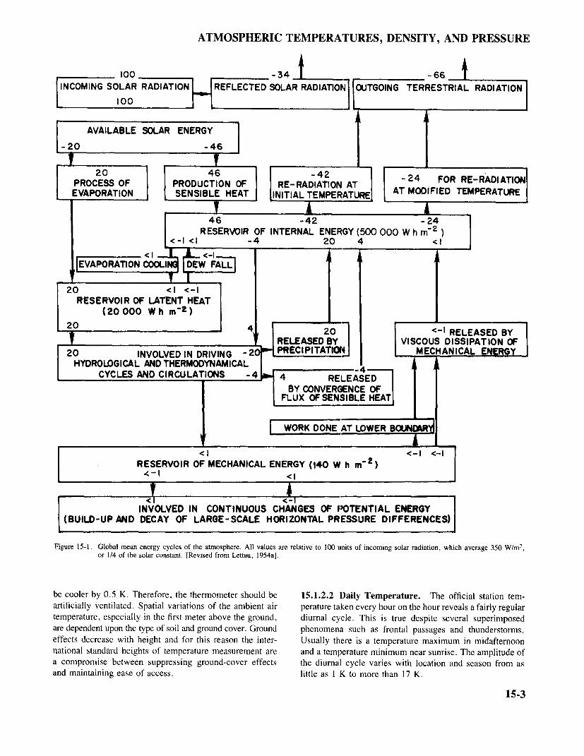
The main features of the global energy transformationare summarized in a flow chart, Figure 15-1, from whichthe relative importance of the major energy cycles withinthe earth-atmosphere thermodynamic system can be deter- 15.1.2 Surface Temperaturemined. The numerical data presented in this figure are usefulfor various quantitative estimates. For example, if all energy 15.1,2.1 Official Station Temperature. The standardinputs for the system ceased and rates of energy expenditure station temperature used in meteorology [NWS, 1979] iswere maintained, the reservoir of mechanical energy (mo- measured by a thermometer enclosed within a white-painted,mentum) would be depleted in about 3 days, the reservoir louvered instrument shelter or Stevenson Screen. The shelterof latent heat (precipitable water) in about 12 days, and the has a base about 1 m (1.7 to 2.0 m in Central Europe) abovereservoir of internal energy (heat) in about 100 days. the ground and is mounted in an open field (close-cropped

Although an absolutely dry and motionless atmosphere grass surface). The standardized height of the thermometeris conceivable, it is difficult to imagine an atmosphere at is about 1.8 m. The shelter permits air circulation past thezero degrees K. It is perhaps more appropriate to interpret thermometer and is designed to exclude direct solar andthe above time intervals as fictitious cycles of turnover of terrestrial radiation. However, the shelter unavoidably ab-the atmospheric properties. The relative magnitudes of these sorbs and radiates some heat energy which, although min-life cycles show that, in comparison with rainfall and winds, imal, causes some deviation of the thermometer readingtemperature is the most conservative and will exhibit the from the "true" air temperature. On calm, sunny days therelatively smallest, and thus most regular, temporal and recorded daytime shelter temperature will normally be 0.5spatial large-scale variation. to 1 K higher than the free air temperature outside the shelter

The solar energy input into the atmosphere at any one at the same level. On calm, clear nights it will most likely

15-2

ATMOSPHERIC TEMPERATURES, DENSITY, AND PRESSURE

10 - 34 ~ -66 1INCOMING SOLAR RADIATION REFLECTED SOLAR RADIATION OUTGOING TERRESTRIAL RADIATION

O00

AVAILABLE SOLAR ENERGY

-20 -46

PROCESS OF PRODUCTION OF RE-RADIATION AT 4 FOR RE-RADIATION_EVAPORATION SENSIBLE HEAT INITIAL TEMPERATURE AT MODIFIED TEMPERATURE

46 -42 24RESERVOIR OF INTERNAL ENERGY (500 000 W h m- 2 )

<-I <I -4 20 4 <1

<lI_ JL_ <-I AREVAPORATION VCOOLIS DDEW FAOLL

M I E20 <1 <-I

RESERVOIR OF LATENT HEAT(20 000 W h m 2 )

20 4 2 RELEASED BY

20 INVOLVED IN DRIVINUG PECIPITATION MECP ANICAL ENERGHYDROLOGICAL AND THERMIODYNAMICAL_ ICYCLES AND CIRCULAAIONS -4C R P D RENES)or 1/ fhslrconatnt [Revsed ro Lttao95aBY CONVERGENCE OF I

FLUX OFSENSIBLE HEATJ

| WORK DONE AT LOWER BOUNDARA

<1<-<-RESERVOIR OF MECHANICAL ENERGY (140 W h m- 2 )

4-1~~~~~~~<

~~~~~<1

INVOLVED IN CONTINUOUS CHANGES OF POTENTIAL ENERGY(BUILD-UP AND DECAY OF LARGE-SCALE HORIZONTAL PRESSURE DIFFERENCES)

Figure 15-1. Global mean energy cycles of the atmosphere. All values are relative to 100 units of incoming solar radiation, which average 350 W/m2,or 1/4 of the solar constant. [Revised from Lettau, 1954a].

be cooler by 0.5 K. Therefore, the thermometer should be 15.1.2.2 Daily Temperature. The official station tem-artificially ventilated. Spatial variations of the ambient air perature taken every hour on the hour reveals a fairly regulartemperature, especially in the first meter above the ground, diurnal cycle. This is true despite several superimposedare dependent upon the type of soil and ground cover. Ground phenomena such as frontal passages and thunderstorms.effects decrease with height and for this reason the inter- Usually there is a temperature maximum in midafternoonnational standard heights of temperature measurement are and a temperature minimum near sunrise. The amplitude ofa compromise between suppressing ground-cover effects the diurnal cycle varies with location and season from asand maintaining ease of access. little as 1 K to more than 17 K.

15-3

CHAPTER 15

Table 15-1. Short-wave radiation on horizontal plane, net radiation, and estimated constituents of heat budget at the earth/air interface showing effectof difference in soil moisture caused by rains before 9 August and a dry spell before 7 September 1953 [Davidson and Lettau, 1957].

Radiation (W/m2 )

Mean Local Time 04h 06h 08h 10h 12h 14h 16h 18h 20h

9 August 1953*

Short-wave 0 141 544 733 796 823 537 144 -Net -59 47 364 497 540 525 273 -13 -Flux into soil -40 29 186 63 74 73 28 -65 -Flux into air - 11 - 81 158 176 190 64 - 17 -Heat of evap. - 8 - 97 276 290 262 181 69 -

7 September 1953**

Short-wave 0 54 441 765 870 735 407 44 0Net -54 -32 181 403 488 398 154 -69 -77Flux into soil -44 -25 36 84 95 66 13 -29 -28Flux into air -6 -6 98 230 303 299 114 -30 -39Heat of evap. -4 - 1 47 89 90 33 27 -10 -10

*Mean soil moisture in 0 to 10 cm layer, about 10% wet weight basis.**Mean soil moisture to 0 to 10 cm layer, about 4% wet weight basis.

The annual cycle of daily mean temperature ranges from endures for several months of the year, the 24-h cycle ispractically zero near the equator to as much as 40 K in the minimal and the small diurnal variations are controlled pri-temperate zone. As an example, Figure 15-2 shows tem- marily by changing winds and cloudiness. In summer, nearlyperatures at Hanscom AFB, Mass. The middle curve reveals all of the solar energy is expended in melting ice; hence,the annual cycle of the daily mean temperature (actually the the maximum temperature seldom exceeds 273 K. Extra-monthly mean is plotted) and shows an annual range of 25K. The diurnal range, given here by the difference betweenmean daily maximum and minimum in Figure 15-2, is fairlyuniform throughout the year, averaging 12 K.

Superimposed on both the diurnal and the annual cycles 310of temperature are many influences including cloudiness, oprecipitation, wind speed and direction, type of soil, ground 300cover, and aerodynamic roughness of the terrain. In theexample of Figure 15-2, there is a range from the uppermost /1% of the daily maximum to the lowermost 1% of the daily 290 a e

LiJminimum that is 3 times the mean diurnal cycle. The stan- a:dard deviation of hourly temperature averages 5 K. The -range from the uppermost 1% of the maximum temperature 280 _wof the hottest month to the lowermost 1% of the minimum .///temperature of the coldest month in Figure 15-2 is about 22 1/2 times the mean annual cycle. 2

The pattern of surface temperature varies with geo-graphic location. This is illustrated by the statistics of some 260widely scattered stations and even by the statistics of neigh-boring stations (Table 15-2). The annual mean temperatureis generally lowest in the polar regions and highest in the 250 /,equatorial belt. In addition, the mean temperature decreasesgenerally with elevation. The diurnal range is greatest indesert climates and least in oceanic or maritime climates. J F M A M J J A S O N D

The mean annual range tends to be greatest in temperate MONTHclimates and least in equatorial climates. Figure 15-2. Surface temperature at Hanscom AFB, Mass. throughout

In polar regions, where continuous darkness (daylight) the year.

15-4

ATMOSPHERIC TEMPERATURES, DENSITY, AND PRESSURE

Table 15-2. Temperatures at various stations around the world.

Mean Mean Hottest ColdestAnnual Diurnal Annual Month 1% Month 1%

Elev. Mean Range Range of Daily of DailyStation Lat Long m K K K Max K Min K

Hanscom AFB, Mass. 42°28'N 71°17'W 43 282.3 11.7 25.6 311 247Boston, Mass. 42°22'N 71°02'W 5 283.8 8.6 24.3 - -Blue Hill Obs., Mass. 42°13'N 71°07'W 192 282.3 9.6 24.4 - -Nantucket, Mass. 41°15'N 70°04'W 13 282.7 7.2 20.4 - -Pittsfield, Mass. 42°26'N 73°18'W 357 280.2 11.4 25.6 - -Worcester, Mass. 42°16'N 71°52'W 301 281.2 9.5 25.4 - -Thule, Greenland 76°32'N 68°42'W 59 261.8 6.4 31.9 289 233Eielson AFB, Alaska 64°41'N 147°05'W 170 270.2 10.8 39.6 303 224Keflavik, Iceland 63°58'N 22°36'W 50 278.1 4.4 11.2 291 258Goose Bay, New Foundland 53°19'N 60°25'W 44 273.2 9.5 33.7 307 237Berlin, Germany 52°28'N 13°26'E 50 282.8 7.2 20.6 307 254Limestone; Maine 46°57'N 67°53'W 230 276.9 9.4 29.4 308 241Boiling AFB, Wash. D.C. 38°49'N 76°51'W 20 287.0 10.2 23.0 311 259Scott AFB, Ill. 38°33'N 89°51 'W 138 286.1 6.2 26.3 311 250Blytheville, Ark. 35°58'N 89°57'W 81 278.4 6.8 17.9 312 255Riverside, Calif. 33°54'N 117°15'W 461 292.7 16.8 14.4 314 269Tucson, Arizona 32°10'N 110°53'W 809 289.4 11.7 19.0 316 267Ft. Huachuca, Arizona 31°25'N 110°20'W 1439 290.0 14.8 17.0 312 264Dharan, Saudi Arabia 26°17'N 50°09'E 22 299.8 11.8 19.8 321 276Wheeler, Hawaii 21°29'N 158°02'W 256 295.8 7.5 4.0 305 283Honolulu, Hawaii 21°20'N 153°55'W 12 297.7 6.7 4.2 308 291Guam, Phillipines 13°29'N 144°48'E 82 300.8 1.7 1.7 306 297Diego Garcia Island 07°18'S 72°24'E 2 300.7 3.9 2.0 305 296Canton Island 02°46'S 171°43'W 3 300.7 1.2 0.8 305 297

tropical regions characteristically have distinct diurnal and version, as much as 4 or 5 K, in the air within several feetannual cycles. These cycles are superimposed over tem- of the ground.perature variations caused by shifting air masses and frontal The induced temperature in military equipment exposedpassages. In tropical regions, the diurnal range rarely ex- to the sun's heat will vary greatly with physical propertiesceeds 6 K. such as heat conductivity, reflectivity, capacity, and type

Depending on circumstances and ground characteristics, of exposure. Surface and internal temperatures, such as arethe surface air temperature could differ by several degrees induced in a boxcar, make the reading of the shelter ther-over short distances ranging from a few meters to a few mometer only the beginning of the engineering problem.kilometers. Also, vertical temperature variations are ob- Table 15-2 is only an initial guide to the effects ofserved from a few millimeters above the ground to the top various influences on station temperature. Detailed temper-of the instrument shelter. On windy, cloudy days or nights, ature information should be obtained from the climatologicalthe differences between thermometer readings, within short record of each station or of stations close by. The latterdistances of one another in either the horizontal or the ver- should be modified for the influences of terrain proximitytical, will be minimal. In high temperature regimes, how- to water, and elevation.ever, with a bright sun and light winds, the ground surface,especially if dry sand, can attain temperatures 17 to 33 K 5.1.2.3 Horizontal Extent of Surface Temperature.higher than the free air. The temperature of air layers within Horizontal differences in surface temperature can arise botha few centimeters of the surface will differ only slightly from large-scale weather disturbances and from local influ-from the ground, but the decrease with height is rapid. The ences. Weather disturbances such as cold and warm fronts,temperature at 0.5 to 1 m above the ground will be only thunderstorms, and squall lines account for unsystematicslightly warmer than that observed in the instrument shelter changes in the horizontal temperature gradient. Nonuniformat 1 or 1.5 m above the ground. Conversely, on calm, clear radiational heating and cooling of the ground also contributenights the ground radiation can produce a temperature in- to turbulent mixing, cloudiness, and vertical motions in the

15-5

CHAPTER 15

Table 15-3. Estimates of the horizontal scale of certain local meteorological conditions.

Horizontal Scale Temperature DifferencesLocal Conditions (km) (K)

Changes in Air Mass 160 to 1600 3 to 22Weather Fronts 16 to 160 3 to 22Squall Lines 8 to 80 3 to 17Thunderstorms 8 to 24 3 to 17Sea Breezes 8 to 16 1 to 11Land Breezes 3 to 8 1 to 6

lower troposphere, resulting in constantly changing tem- lower. Also, some pronounced horizontal temperature gra-peratures at the surface. dients occur along coastlines in temperate latitudes due to

Horizontal transport by air currents, referred to as ad- the cooling effect of coastal sea breezes.vection, is a key factor in surface temperature differences. Generally, temperatures between two stations becomeLarge-scale advection will bring both the relatively dry cold more independent of one another with increasing distancearctic air masses and the relatively moist warm tropical air (Figure 15-3). One model curve [Gringorten, 1979] for fit-masses alternately to the temperature zones. This can pro- ting the correlation coefficient p as a function of distance sduce large changes in the day's mean and the diurnal range between stations is given byof temperature.

Table 15-3 gives estimates of surface temperature dif- 2p = -[(cos -] (x) - /1 - ca2] , (15.1)ferences over varying horizontal distances associated with p - ' (- (15)

several kinds of weather phenomena. Large-scale differ-ences are greatest in winter due to the more substantial wheredifferential heating by solar radiation from equator to poleand, consequently, the more intense large-scale motion of sthe atmosphere. In summer the north-south gradients in solar a = 128r (15.2)insolation are much less, but the general increase in theamount of insolation results in more thunderstorms and other where r is the model parameter and is in the same units asair-mass activity. the distance s. The value of r is, in fact, the distance over

Systematic differences in the surface temperature be- which the correlation coefficient is 0.99. For the curve intween neighboring stations are due to five prime factors: (1) Figure 15-3, r = 17.7 km. While this curve could be fittedaspect or orientation of the terrain with respect to incident by other models, the given model curve has the quality thatsolar radiation, (2) type of surface structure and of soil coverunderlying the stations, (3) proximity to the moderatinginfluences of large water bodies, (4) elevation, and (5) dif- 10ference in solar time for stations that are several hundredkilometers apart. Sometimes the topography permits "pools" 9of cold air to drain locally at night into lower basins or .8Z~~~valleys. Also nonuniform distribution of water vapor and W 7

Ucloudiness will result in uneven distributions of short-wave L.

and long-wave radiation and, consequently, uneven cooling \and heating at the surface. Z~~~~~~

A striking example of local influences on surface tem- 4perature gradients is found in the temperature contrasts be-tween cities and the surrounding countryside. The sheltering .2

effect of buildings, their heat storage, products of fuel com-bustion, smog, rain water drainage, and snow removal all

0act to make the city a relative heat source. Thus, the city'si i i I I i J I J a Inightly minimum temperature might be 5 to 14 K higher -0 200 400 600 800 1000ooo 1200 1400 1600 8oo00 2000 2200 2400

than that of surrounding suburbs. As another example, in DISTANCE (km)hilly or mountainous terrain the valley floor could have a Figure 15-3. The correlation coefficient of the daily mean temperature ofdiurnal temperature range 2 to 4 times as great as that over Columbus Ohio with that of nine other U.S. stations atthe peaks, and a temperature minimum from 5 to 17 K indicated distances from Columbus.

15-6

ATMOSPHERIC TEMPERATURES, DENSITY, AND PRESSURE

the correlation coefficient decreases exponentially with dis- northerly latitudes during the winter months when the tem-tance between stations for the first few kilometers of sep- perature distributions are substantially bimodal. Thus thearation. Eventually, the correlation coefficient drops to zero straightforward method for determining the frequency dis-at distance 128r. tribution of hourly temperatures is to obtain a representative

In the United States the separation between weather sample of observations for each location and compute thestations averages about 160 km, with the exception of the distributions. Estimates of the frequency distribution fromeastern states where it is 30 to 80 km. The root mean square such data can be made using the Blom formula given bydifference of temperatures, as a function of the correlationcoefficient p between two stations is approximated by P(T) = / (15.4)

N + 1/4' (54rmsd = st 2(1 - p), (15.3)

where P(T) is the estimated cumulative probability of thewhere s, is the standard deviation of the hourly temperature temperature T, nT is the number of observations equal to(estimated as 5 K for Hanscom AFB). For stations 150 km or less than T, and N is the overall sample size. Since,apart, with p = 0.91 (Equation 15.1), the rmsd should be representative samples of data are not easily obtained forapproximately 2 K. regions outside North America, an objective method has

been developed by Tattelman and Kantor [1977] so that the15.1.2.4 Runway Temperatures. At airports the desired frequency distribution of surface temperature can be esti-length of the landing strip or runway is directly related to mated at all locations from data in climatic summaries thatair temperature. Any discrepancy, therefore, between free are available for most locations throughout the world.air temperature over runways and shelter temperatures is Because the warmest temperatures in the world are foundimportant in establishing safe aircraft payloads and runway at locations where the monthly means are high and the meanlengths. It had been thought, on days when insolation is daily range is large, Tattelman et al. [1969] developed anstrong, that the free air temperature over airfield landing index using these values. The index is expressed bystrips is significantly higher than standard shelter temper-ature over the surrounding grassy areas. Results of obser- lw = T + (Tax - Tnin), (15.5)vations, however, over four airstrips (Easterwood Airport,Hearne Air Force Satellite Field and Bryan Air Force Base where Iw, is the warm temperature index, T is the monthlyin Texas, and an auxiliary naval airstrip near Houma, Lou- mean, Tmax is the mean daily maximum, and Tmin is theisiana) have shown that the air between 0.3 and 6 m above mean daily minimum temperature (K - 273) for the warmesta landing strip is about 0.5 K cooler than indicated by the month. The index was related to temperature occurring 1%,shelter thermometer over adjacent grassy areas. The relative 5% and 10% of the time during the warmest months at asmoothness of the runway surface is the physical cause of number of locations; it appears in the following regressiondaytime flow of air from grass to runway. During the tran- equations for estimating monthly 1%, 5% and 10% warmsition from flow over the rough grassy surface the wind temperature extremes [Tattelman and Kantor, 1977]:speeds up and entrains the cooler air immediately above therunway. When a daytime equilibrium state is established, T = 0.6761W + 10.657, (15.6)there will be a large lapse rate close to the ground. This isthe effect over both concrete and blacktop airstrips with T% = 0.7331w + 5.682, (15.7)surrounding grass having only a slightly modifying effect.

In exceptional cases the free air temperature over the 0762 + 2.902. (15.8)runway exceeds the shelter temperature but by no more than where is the estimated temperature in (K - 273) occurring0.5 K when averaged over 10 min, 1 K when averaged over

1, 5, and 10% of the time, respectively. The same principle1 min with a dry soil environment, and 0. 25 K (5-min mean)can be used to estimate cold temperature extremes. The coldwith a swamp environment. Thus the standard method oftemperature index istemperature measurement in a properly exposed shelter over temperature index is

grass provides a representative temperature for the esti-mations of runway length and aircraft payloads. Ic = T - (Tn.ax - Tmam), (15.9)

15.1.2.5 Temperature Extremes. A knowledge of the where Ic is the cold temperature index, T is the monthlyoccurrence of hot and cold temperature extremes is impor- mean, Tmax is the mean daily maximum, and Tmin is thetant for the design of equipment and the selection of material mean daily minimum temperature (K - 273) for the coldestthat will be exposed to the natural environment. The hourly months. The corresponding regression equations [Tattelmantemperature observations at most locations are not normally and Kantor, 1977] aredistributed around the mean monthly values. Departuresfrom a normal distribution are largest in the temperate and T1o% = 1.069Ic - 7.013, (15.10)

15-7

CHAPTER 15

15% =1.0841 - 3.050, (15.11) Most extreme high temperatures have been recordednear the fringes of the deserts of northern Africa and south-

Tio% = 1.082Ic - 0.704. (15.12) western U.S. in shallow depressions where rocks and sand

reflect the sun's heat from all sides. In the Sahara, theThis technique has been used by Tattelman and Kantor greatest extremes have been recorded toward the Mediter-

[1976a,b] to map global temperature extremes using loca- ranean coast, leeward of the mountains after the air hastions for which monthly climatic temperature summaries are passed over the heated desert. The highest temperature onavailable. Estimates of the 1% warm and cold temperature record is 331 K at Al Aziziyah, Libya (32°32'N, 13°1'E,extremes for the Northern Hemisphere are shown in Figures elevation 112 m). Northern Africa and eastward throughout15-4 and 15-5. most of India is the hottest part of the world, Large areas

I~~~~~~~~~~~~3~~~~~

Figure 15-4. Temperature equaled or exceeded 1 % of the time during the warmest month (K -273) [Tattelman and Kantor 1976a].15-8 3 -;- 3 .. 45o

%.~?,8,/ ~~~~~~~~

34~~~~~~~~~~~~~~~~~~~~~

,~t- - _ ,~~~~~~~l 1,;,

io-\~~~~~~~~~~~~~~~~~~~~~-

Figure 15-4. Temperature equaled or exceeded 1% of the time during the warmest month (K -273) [Tattelman and Kantor, 1976a].

15-8

ATMOSPHERIC TEMPERATURES, DENSITY, AND PRESSURE

0~~~~I

4- /1~~~~~~~~- 54I~~~~~~~~~~~~~~~~~~~~~3./ ---.. 0

~~~~~-40\ "0 '\ 10"% .~i

-25~ ,~~~~~~~~~

$ . < X' .'

Figure 15-5. Temperature equaled or colder 1% of the time during the coldest month (K -273) [Tattleman and Kantor, 1976al.

attain temperatures greater than 316 K more than 10% of equal to or greater than 316 K for 1% of the time in thethe time during the hottest month. Sections of northwest hottest month. Death Valley. within this area, has temper-~'2'~~~~~~~~~~~~~4 -40, -3 2:5 1..

,,'3, 0 ~ 4 -50 :1.5

~45~~~~~~~~~~3 2 i_2

Africa experienced temperatures greater than 322 K as much atures equal to or greater than 322 K for 1 % of the time inas 1% of the time during the hottest month of the year. the hottest month and it once had a record temperature ofRegions in Australia and South America have temperatures 330 K.

Fat and above 311 K much of the time, but do not experience Geographic areas of extreme cold include the Antarcticattain temperatures greater than 316 K more than 1% of the time Plateau (2700 to 3600 m in elevation),% of the central part ofthethe time during the hottest month. Sections of northwest hottest month. Death Valley, within this area, has temper-Africa experienced temperatures greater than 322 K as much atures equal to or greater than 322 K for 1% of the time inas l% of the time during t he hottest month of the year. the hottest month and it once had a record temperature ofRegions in Australia and South America have temperatures 330 K.at and above 31 1 K much of the time, but do not experience Geographic areas of extreme cold include the Antarctictemperatures greater than 316 K more than 1% of the time Plateau (2700 to 3600 m in elevation), the central part ofduring the hottest month. The southwestern U.S. and a the Greenland Icecap (2500 to 3000 m), Siberia betweennarrow strip of land in western Mexico are exceptionally 63°N and 68°N, 93°E and 160°E (less than 760 m elevation)hot. A substantial part of the area experiences temperatures and the Yukon Basin of Northwest Canada and Alaska (less

15-9

CHAPTER 15

than 760 m elevation). The generally accepted record low bility PT of the annual extreme temperature, it is equal totemperature (excluding readings in Anarctica) is 205 K in 1/(1-PT) years. The return period is not to be confused withSiberia. the planned lifetime (n) of the equipment. Roughly speak-

ing, the temperature with the 100-yr return period or the15.1.2.6 The Gumbel Model. For equipment that is either annual 1% (PT = .99) is approximately the 10% temper-in continuous operation or is on standby status, thereby ature of a 10-year planned life.continuously exposed to all temperatures, the statistic of The Gumbel distribution with a set of periodic extremesinterest is the extreme temperature that is likely to occur is the easiest model to use, but there are reservations in itsduring a full month, season, year, decade, or whatever application. Theoretically the basic distribution, such as theperiod is considered to be the useful lifetime of the equip- station temperature taken hourly, should be an exponentialment. type, such as Pearson Type III or Gaussian. However, this

Many extreme values have been estimated effectively condition may not be sufficient because the record may notby a model that has become known as the Gumbel distri- be long enough to make the annual extreme fit into a Gumbelbution. Let us assume the annual highest temperature (Ti) distribution. The Gumbel distribution is only the limitinghas been recorded for each of N years (i = 1 ,N) with av- form over long times and may not be adequately reachederage T and standard deviation st The Gumbel estimate of over short periods. It is advisable, therefore, to test the datathe cumulative probability PT of the annual extreme high to determine if the Gumbel distribution is applicable. Figuretemperature (T) is then 15-6 illustrates the use of special-purpose "Extreme Prob-

ability Paper" in which the cumulative probability PT is readPT = exp[-exp(-y)], (15.13) on the vertical axis to correspond to T on the horizontal

axis. Alongside the scale of PT is the scale of the reducedwhere variate y, which is uniform on this paper. A Gumbel dis-

tribution appears as a straight line.Let us suppose a set of N extreme temperatures Ti for

Y = s - (T - T), (15.14) each of N years (i = 1,N) is ordered from lowest to highestStvalue. The cumulative probability of the ith lowest tem-

where, to five decimal places perature since it is an extreme is best estimated by

= 0.57722andOy =, 1.28255. (15.15)

(There are other estimates to the Gumbel distribution. Thisone is preferred for its simplicity as well as degree of ac- 4 _ .98curacy.) The quantity y is referred to as the reduced variate.

- .97·If one is interested in the cold temperature, these formulashold with the T and T reversed in Equation (15.14). 3 -- .90

If the lifetime of a piece of equipment is intended to ben years, then the cumulative probability PT(n) that the tem- >8

-. 8 Operature T will not be exceeded in the n years is ' 2

F-PT(n) = exp[-exp(-y -- + en n)] (15.16) -. 7 -

where y is given by Equation (15.14). Assuming, for ex- I - .5 <W~~

ample, that we want to estimate the temperature T that has o o0- .3only a 10% probability or risk of being exceeded over n Q .

years, we set PT(n) equal to 0.9 in Equation (15.16) and a O--.solve Equation (15.16) for y obtaining

y = fnn - fn(-fn P), (15.17) - .-05-. 01

which we in turn use in Equation (15.14) to obtain .001

-2 i5'=T + st(y .~) /T= T + 'sy - (15.18) 300 305 310 315

TEMPERATURE, T (K)

The return period is a term sometimes used in associ- Figure 15-6. a) Annual highest temperature, Hanscom AFB, Mass., 21ation with the extreme. In terms of the cumulative proba- ordered values (1944-1964).

15-10

ATMOSPHERIC TEMPERATURES, DENSITY, AND PRESSURE

TEMPERATURE

.98

.97 300K

3 .95290K DEW POINT

>' - .9 9,,2 2 6- 280K 24

·8 I'-" 40% - RELA~iV~,~4

:_: 7 .3O

.5 o 0%

rathTerEATRE (K) 205N n e l FMPS,II

Figure 15-5 b) Lowest temperatures of 22 winter med-a5 02 04 0 0t 1 12 1 6u22 02

Figure 15-7. Yuma, Arizona typical July diurnal cycles when maximumi - 0.44 (51)daily temperature equals or exceeds 317 K (based on

is =N + 0.3012 K1 9 an1961-1968 data).

rather than Equation (15.4). Now in the example of Figure15-6a, we have the plot of the annual highest temperatures The dewpoint has a median of 287 K with a small diurnalof 21 years (1944-1964 at Hanscom AFB, Mass.) ordered range. Relative humidity, consequently, has a large-ampli-from lowest to highest value and having cumulative prob- tude diurnal cycle. Wind speed at anemometer levels of 6ability estimates PT given by Equation (15.19). The mean to 8 m above ground averages approximately 4 m/s withis T = 309 K and the standard deviation is s1 = 1.9 K. little diurnal range. Solar insolation, on the other hand, hasThe solution of Equation (15.14) gives the straight line plot a large diurnal range with a maximum clear-sky value ofbetween y and T as shown. Whether the straight line and 88.2 L/h and a minimum value of zero from 2000 LST intherefore the Gumbel distribution adequately fits the distri- the evening till 0500 LST in the morning. For the hottestbution is a matter of judgment. If accepted, and it should areas on earth (for example, Sahara Desert) Table 15-4be in this example, then the 99th percentile (PT = .99) or presents the associated cycles of temperature, relative hu-the 1% extreme is estimated by Equations (15.17) and (15.18) midity, windspeed and solar insolation when the afternoonwith n = I as 315 K. For a lifetime of 25 years (n = 25) temperature in the middle of a 5-day period reaches 322 Kthe temperature of 10% risk (PT = 0.9) is given by Equa- which occurs about 1% of the time in the hottest month.tions (15.17) and (15.18) as 316 K. Death Valley, California is also one of the hottest areas

As another example, Figure 15-6b shows the plot of the but is close to 60 m below sea level resulting in extremeextreme low temperatures of 22 winter seasons (1943-1965) absorption of solar radiation before it reaches the ground.

at Hanscom AFB, Mass. The mean is T = 251 K and the Consequently its maximum clear-sky solar insolation of 82.5standard deviation is s1 = 3.68 K. A straight line fit of L/h is less than that shown in Figure 15-7. Solar insolationthese data is not satisfactory. Possibly a concave curve would I increases with elevation roughly in accord with the ex-be more appropriate. The Gumbel model is not acceptable ponential model given byin this case, and consequently another model should be tried.

i= 1e -p- Pl) (15.20)5.1.2.7 Temperature Cycles and Durations. High tem-perature extremes are inevitably part of a well pronounced where p and p1 are, respectively, atmospheric surface pres-diurnal cycle, modified by wind and by moisture content. sures for a given station and another reference station atTypical of a hot climate, the record of Yuma, Arizona roughly the same latitude I1 is the solar insolation at the(32°51'N, 1 14°24'W) (Figure 15-7) reveals a mean diurnal reference station, and the value for a is dependent on thetemperature range of 15.3 K for the middle 20 days in July. location. For Yuma and Death Valley, where the mean

15-11

CHAPTER 15

Table 15-4. Diurnal cycles of temperature and associated other elements for days when the maximum temperature equals or exceeds the operational 1%extreme temperature (322 K) in the hottest month in the hottest area.

Time of Day (h)

Item 1 2 3 4 5 6 7 8 9 10 11 12

Temperature (K)

Hottest Day 308 307 307 306 306 305 306 308 311 314 316 3171 day before 309 308 307 306 306 305 306 309 311 313 315 317

or after2 days before 307 307 306 306 305 305 306 308 310 312 314 315

or after

Other Elements

Relative Humidity(%) 6 7 7 8 8 8 8 6 6 5 4 4(dp = 266 K)

Windspeed (m/s) 2.7 2.7 2.7 2.7 2.7 2.7 2.7 2.7 2.7 4.3 4.3 4.3Solar Radiation 0 0 0 0 0 5 23 43 63 79 90 96

(L/H)

Time of Day (h)

Item 13 14 15 16 17 18 19 20 21 22 23 24

Temperature (K)

Hottest Day 320 321 321 322 321 321 319 315 314 312 311 3101 day before 318 320 320 321 320 319 317 315 313 311 310 309

or after2 days before 316 317 319 320 319 318 317 314 312 311 310 309

or after

Other Elements

Relative Humidity(%) 3 3 3 3 3 3 3 4 5 6 6 6(dp = 266 K)

Windspeed (m/s) 4.3 4.3 4.3 4.3 4.3 4.3 4.3 4.3 4.3 4.3 4.3 2.7Solar Radiation 96 90 79 63 43 23 5 0 0 0 0 0

(L/H)

atmospheric surface pressures are about 1006 mb and 1020 amount in June. In contrast, Table 15-6 gives correspondingmb respectively, a = 0.00461 mb-1. results for the insolation at Caribou, Maine where there is

The hottest locations in the Sahara Desert are relatively much more frequent cloudiness and precipitation.high (about 300 m above sea level) with atmospheric pres- The operability of equipment in a cold climate is verysure about 977 mb. Thus Equation (15.20) yields an estimate much dependent on the duration of extreme cold. Unlikefor the peak solar insolation at these elevations of about 100 the hot extremes, cold extremes are usually accompaniedL/h. Most countries, however, including the U.S., Canada, by very small diurnal ranges, if any. The direct approachand the United Kingdom, have adopted a peak figure for for determining the duration of cold temperature is by ansolar insolation for operational and design purposes of 96 analysis of hourly data. Such data are available for manyL/h. stations in North America but are not generally available

Heavy clouds and precipitation reduce the incident solar for other regions of the world. Data from 108 stations ininsolation. At a few stations the National Weather Service the U.S. and Canada have been analyzed [Tattelman, 1968]has taken records of incoming solar insolation. Table 15-5 to obtain information on the longest period of time duringgives the results of processing such data from Albuquerque, which the temperature remained at or below eight "thresh-N.M. It presents estimates of the probabilities with which old" values (from 273 K to 220 K) during a 10-yr period.daily incoming solar insolation equals or exceeds the given Figure 15-8 from that report shows the results for a threshold

15-12

ATMOSPHERIC TEMPERATURES, DENSITY, AND PRESSURE

Table 15-5. Probability of daily solar insolation equaling or exceeding 8 ;.i t - eo .7'

given amounts for given number of consecutive days in June, X, . |

at Alburquerque, N.M. Station elevation is 1620 m. Peak 'o,- .clear sky solar insolation was observed at 910 L/day. ' .:j. ' :

Insolation No. of Consecutive Days · 0

L/Day 1 2 4 8 15 30 .. " , ... . .-

850 0.03 ' . , i i .800 0.24 0.06750 0.49 0.28 0.09700 0.71 0.54 0.31 0.11 .... I..... ' '650 0.81 0.70 0.52 0.29 0.09 > . .600 0.90 0.84 0.77 0.52 0.29 0.08 ot , .o 0

550 0.935 0.90 0.81 0.65 0.44 0.20 /. , , ;500 0.955 0.93 0.87 0.75 0.57 0.33 , . .450 0.971 0.95 0.91 0.82 0.67 0.43400 0.985 0.972 0.946 0.87 0.81 0.65 '/V350 0.9933 - 0.973 0.945 0.902 0.82 .300 0.9946 - 0.980 0.958 0.928 0.86 f . ,250 0.9975 - - 0.980 0.963 0.932 ! , / , " .200 0.999 - - - - 0.970 ·\ ' ,

/ , ''. l i. ., , ' 0

.... ' \ ... . . . \ -<.a , , '. '''' '''' GENE RALLY < 1.5 k m I .,, .X:,-' .... ...'

"' ' / '° ' ' " 'l As 'f ' "" [

' 70° "'10,

Table 15-6. Probability of daily solar insolation equaling or exceeding Figure 15-8. Longest duration (h) of temperature < 250 K in ten wintersgiven amounts for given number of consecutive days in June, [Tattelman, 1968].at Caribou, Maine. Station elevation is 190 m. Peak clearsky solar insolation was observed at 843 L/day.

Insolation No. of Consecutive Days temperature of 250 K. The report also presents the expectedL/Day 1 2 4 8 15 30 (approximately 50% probability) duration of the temperature

850 at or below six "threshold" temperatures (from 273 K to800 0.019 232 K) during a single winter season. Figure 15-9 shows750 0.085 0.02 the single winter results for a threshold value of 250 K.750 0.085 0.0257 Estimates of duration have been made using data that650 0.31 0.13 0.02 consisted mainly of daily, monthly and annual average max-

60 0.40 0.20 0.05 imum and minimum, and monthly and annual absolute max-550 0.47 0.26 0.086 imum and minimum, for some 35 to 50 years at Siberian,550 0.47 0.26 0.1086 0Yukon and Alaskan stations. The mean January temperature500 0.55 0.33 0.13 0.024 in eastern Siberia (Verkhoyansk and Oimyakon) is 225 K.450 0.59 0.40 0.18 0.037 Table 15-7 presents estimates of the lower 20% of the av-400 0.66 0.50 0.26 0.075350 0.72 0.56 0.33 0. 12 0.0 2 erage temperature (averaged for durations ranging from one350 0.72 0.56 0.4733 0.212 0.02 hour to 32 days), the maximum temperature for the durations300 0.78 0.67 0.47 0.22 0.062 shown, and the minimum temperature for the same dura-250 0.82 0.72 0.54 0.30 0.10 tions

200 0.88 0.80 0.66 0.42 0.22 0.05 The duration of temperature anywhere, hot or cold, is150 0.96521 0.9487 0.9077 0.59 0.37 0.4013 of general interest. In the midlatitude belt the temperatures100 0.965 0.96 0.92 0.84 0.72 0.51 of Minneapolis, Minn. are typical (Figure 15-10). The Jan-

80 0.980 0.962 0.93 0.86 0.75 0.56 uary probability distribution of all hourly temperatures has80 0.980 0.97 0.95 0.9 0.8 0.7 a 1% value of 244 K, and a 50% or median value of 263

70 0.987 0.978 0.956 0.912 0.83 0.70.70 0.987 0.7 0.956 0.912 0.83 0.70 K. That is, the range from the lower 1% to the median is60 0.9931 - 0.971 0.947 0.903 0.8250 0.9961 - -09 0.977 0.95 0.90 19 K. The 24-h averages, as expected, have a narrower

40 0.99906 - - - - 0.97 range, 17 K. The range of monthly averages (768 h) is muchnarrower, 7 K. Similarly, the July hourly temperatures have

15-13

CHAPTER 157~~~~~. M.8010 -

99YI7O~~~~~~~~~~~ ~ ~~~~~ 310 ~~~~~~~~~~~JULY

6o' :'\ ~ ~~ ,, , ,- 5'~~~~5 /1~~~~~~~~9

so JANUARY

too

- .' ' ' ~ '<i r4 ' X -- ~... .. i.-'" ," '.." | I HOURS 3 6 12 24 48 96 192 364 768

". .,~. .. \ ....i ~ , . ~. ,2. . . " 0 .- Figure 15-10. The distribution of the averages of consecutive hours of[d\~ "~/, l.~ ~ ~~~ ~~~~ ' < . ....... ...... ...2 0 ' ] temperature at Minneapolis, Minn. (The upper half is for

:'' 's \'v: -' , . ~_..: ' .', i77'h I mid-summer month, from 1 July to I August; the lowerhalf is for mid-winter month, I January to I February.

l~@/i~, '.~4~.i _ '~ .' "-~ ~ ~~.'~i'. '"] ~~ Each curve is labeled with percent probability of occur-rence.)

40

[ 've 'x ,/e. .... . ,S ' i AABY .. /.~~~~~~~ 1 ~month of January, and 0.919 in the midsummer month of} .'/ "" -,'~ -~~~~~ ~ ' :~ :+.' a / "CJuly.

it r .\i"x .i: '" .. ' .... '- L'A; Hourly observations have been taken at Minneapolis for[ ;, Ad ' \' a''.' "' X' '. many years, making many useful summaries possible. Fig-t'" ,'- .'\ .': '. .... ' .. " . ure 15-11 shows a sample distribution (1949-1958) of hourlyLY <, 5 A .... . .: . , ....... ' January temperatures alongside the left axis and the distri-

|GNRALLY <." 1/.5 !' i ) : .b.: .. '~'... ' bution of m-hour minima over the body of the graph, m

[E. ,,. ' o -~ Oo 1 \.. from 1 hour to 768 hours (1 Jan to I Feb inclusive). Figure15-12 shows the sample distributions of hourly temperaturesin January of m-hour maxima. As an example of the use-

Figure 15-9. Expected longest duration (h) of temperature < 250 K dur- fulness of such a chart, freezing conditions (273 K) areing a single winter season [Tattelman, 1968]. f

shown as 94% frequent for l-h durations. For 24 consecutivehours this frequency reduces to 83%, for 8 days (192 h) to42% and for 16 days (384 h) to 10%.

a 12 K range from the 50% value of 295 K to the upper1% value of 307 K. The 24-h averages have an 8 K range 15.1.3 Upper Air Temperatureand monthly averages have only a 2 K range. These figuresimply a relatively high hour-to-hour correlation. Correlation The temperature data discussed in this section are fromanalysis has provided estimates of 0.982 in the midwinter direct and indirect observations obtained from balloon-bornedirect and indirect observations obtained from balloon-borne

Table 15-7. Durations of cold temperatures associated with the 222 K 9extreme. Each temperature in this table is the maximum,average, or the minimum in an operational time exposure of 9 /9m hours, with 20% probability of occurrence, during Janu- / /ary, in a Siberian cold center.

Time m(h) _

1 3 6 12 24 48 96 192 384 768 o .6 26

Maximum .4Temperature 222 223 224 225 226 228 230 334 238 241. 3 -

K 2.

AverageTemperature 222 222 222 222 222 222 222 223 223 224 .

K.02

Minimum I HOURS 3 6 12 24 48 96 192 384 768

Temperature 222 222 220 219 217 216 215 213 211 210K Figure 15-11. The cumulative probability of the M-hour minimum tem-

perature (1 January to 1 February) at Minneapolis, Minn.

15-14

ATMOSPHERIC TEMPERATURES, DENSITY, AND PRESSURE.98 \_F__T_ X r -I - F FT X 1] T

· ~~~~~~~~~~~~~~~~~~~~~~~~~.935~~~~~~ _WALLOPS TEMPERATURE

.9 60 -

M ~~~~~~~~~~~~~~~~~~~52.6

UJ.5

44 7

.02 ~I 2E / d/ JANI HOURS 4 12 24 48 96 192 284 768 I A

//;/ JULY-- --

Figure 15-12. The frequency of duration (h) of the temperature (< T) in 20 / OCT -....

the mid-winter month (1 January - I February) at Minne-apolis, Minn. (based on 1943-1952 data.)~~~~~~~~~~.3

1236 -~~~~~~~~~~- F.--

instruments, primarily radiosondes, for altitude up to 30 km -- \.and from rockets and instruments released from rockets for 4 _ a d--

altitudes between 30 and 90 km. | I l l l l l180 200 220 240 260 280 300

15.1.3.1 Seasonal and Latitudinal Variations. The TEMPERATURE (K)

Reference Atmospheres presented in Chapter 14 providetables of mean monthly temperature-height profiles, surfaceto 90 km, for 15° intervals of latitude between the equator

52 52 -instNruethsol.Ths prialyrdoflsondesc foth atithe upasona 30ndand fro rokt an isrument rlased fro rokt fo I4 -l Adv--r-I

| ~ ~ ~ ~ ~ I . I44 ~~~~~~~~~~~~~~~~~44

_36 /_' L6 / A ---- I---18 0 280 APR 240 280 APR 300 180 200 220 240 260 280 30015..31 eaonl ndLaitdialVaiaios.ThEMPRTR TEMPERATURE (K)Figures 15f3 measna difernce thly temperature-atigtud profilesatAcninIld, Wlos I l n , a dF.Curfchil

5125236 -~~~~~~~~~~~~~~~~~~~~~~~~~~~~~~~~~~~~~~~~~~~~~~~~~~~.

F-~~~~~~~~~~~~~~~~~~~~~~~51

CHAPTER 15

Table 15-8a. Median, high, and low values of temperatures for January Table 15-8b. Median, high, and low values of temperatures for Januaryand July at 30°N. and July at 45°N.

1% 10% 20% 1% 10% 20%

Altitude Median High Low High Low High Low Altitude Median High Low High Low High Low

(km) (K) (K) (K) (K) (K) (K) (K) (km) (K) (K) (K) (K) (K) (K) (K)

January January

5 262 272 251 267 256 265 258 5 250 263 233 257 239 254 242

10 229 239 219 235 223 233 225 10 220 233 206 227 212 225 21415 208 221 198 216 203 214 205 15 217 231 202 225 208 222 211

20 208 222 200 216 203 214 204 20 215 227 203 222 208 220 210

25 220 231 210 226 216 224 217 25 215 233 197 226 205 224 20930 229 239 218 236 224 234 226 30 221 240 209 230 214 226 21935 240 254 222 248 232 245 235 35 233 258 215 251 223 243 226

40 252 270 240 262 249 258 250 40 247 272 226 264 236 257 240

45 264 283 253 277 258 272 260 45 262 288 240 283 250 271 254

50 266 281 256 276 260 273 262 50 265 282 249 274 256 270 258

55 254 272 231 267 243 263 248 55 253 275 229 267 239 263 245

60 243 254 223 248 232 246 235 60 244 266 220 263 230 257 24165 231 254 218 242 226 238 228 65 235 255 214 246 223 243 228

70 220 235 198 227 204 225 210 70 226 246 206 238 211 234 21775 218 253 197 237 203 227 208 75 225 261 197 245 205 235 21080 209 243 187 230 194 217 197 80 216 248 185 237 197 228 202

July July

5 272 278 262 274 266 275 268 5 267 277 255 274 259 272 26210 238 249 227 246 232 242 234 10 235 247 222 240 227 239 23015 204 216 196 211 200 210 200 15 216 227 205 222 206 220 212

20 212 223 203 218 206 216 206 20 219 233 207 227 213 225 21525 223 230 216 227 218 226 219 25 225 233 216 229 217 228 221

30 234 241 226 238 229 236 231 30 234 242 228 239 231 237 23235 244 254 237 250 240 247 242 35 245 254 238 250 241 248 24340 256 267 247 263 251 261 253 40 256 268 250 265 254 263 255

45 266 275 259 272 264 269 265 45 268 280 260 276 263 272 26550 269 282 258 278 262 275 264 50 273 283 264 279 268 277 27055 264 273 247 269 253 267 256 55 264 273 249 269 255 267 260

60 247 262 231 255 240 252 243 60 247 270 230 264 235 260 238

65 228 240 215 236 219 234 222 65 230 245 216 241 223 238 22070 209 222 186 219 194 214 200 70 213 226 188 219 196 216 202

75 200 218 178 214 192 209 196 75 195 210 175 205 186 201 190

80 193 207 182 200 189 198 191 80 183 203 154 195 163 191 170

latitudinal variations in mean monthly temperatures. The Temperature-altitude profiles, surface to 60 km, for the mid-largest seasonal variations in temperature occur at altitudes season months at Ascension Island, 8°S, Wallops Island,between 70 and 80 km near 75°N latitude. In this region 38°N, and Ft. Churchill, 59°N, are given in Figure 15-13

the mean monthly temperature fluctuates from 230 K in and illustrate the magnitude of the seasonal and latitudinalJanuary to 160 K in July. In the upper mesosphere, 60 to variations in mean monthly temperatures.85 km, mean monthly temperatures decrease toward the polein summer and towards the equator in winter. In the upper 5.1.3.2 Distribution Around Monthly Means andstratosphere, 20 to 55 km, conditions are reversed; tem- Medians. The distributions of observed temperatures around

perature decreases toward the pole in winter and toward the the median values for altitudes up to 80 km in January and

equator in summer. At altitudes between 15 and 20 km July at 30° , 45° , 600 and 75°N are shown in Tables 15-8atemperature decreases toward the equator in all seasons. to 15-8d. Median, and high and low values that are equaled

15-16

ATMOSPHERIC TEMPERATURES, DENSITY, AND PRESSURE

Table 15-8c. Median, high, and low values of temperatures for January Table 15-8d. Median, high, and low values of temperature for Januaryand July at 60°N. and July at 75°N.

1% 10% 20% 1% 10% 20%

High Low i gh Low High Low Altitude Median High High Low High LowAltitude Median (K) (K) (K) (K) (K) (K) (km) (kin) (K) Low (K) (K) (K) (K)

January January

5 240 255 225 249 231 246 234 5 235 246 222 241 229 238 23010 217 231 203 224 209 222 211 10 214 224 202 219 207 217 20915 217 231 203 225 209 222 212 15 209 219 195 213 201 211 20320 215 236 194 226 204 222 208 20 204 225 179 215 189 210 19425 212 241 185 229 197 223 203 25 205 233 181 221 193 216 19830 216 253 203 235 204 225 210 30 209 255 194 231 198 224 20235 221 277 204 259 209 238 214 35 219 256 i99 249 210 236 21340 227 300 206 278 211 246 219 40 229 284 207 256 219 248 22445 243 303 219 282 225 255 231 45 239 281 203 264 224 260 23350 251 289 226 280 240 271 245 50 249 282 201 265 225 259 22955 251 283 225 275 233 256 238 55 255 291 208 262 221 253 22660 243 271 210 261 224 253 234 60 247 303 206 263 213 255 21965 238 262 208 258 218 249 222 65 238 310 186 277 202 263 20970 239 264 212 253 219 249 225 70 242 297 166 277 201 261 20775 232 255 180 249 203 246 213 75 234 289 183 259 201 261 20780 223 248 173 243 195 239 204 80 224 277 165 254 194 240 201

July July

5 260 271 250 266 254 264 256 5 254 264 244 259 248 257 25010 225 238 214 233 219 231 221 10 229 238 219 234 223 232 22515 225 235 217 231 221 229 223 15 230 237 225 235 228 233 22920 225 233 219 230 222 229 223 20 230 237 227 235 228 234 22925 229 236 222 233 225 232 226 25 230 240 226 238 227 237 22930 239 245 232 243 234 241 235 30 243 262 233 247 235 246 24035 252 258 243 256 247 253 248 35 256 262 238 260 246 258 25040 265 272 259 269 263 268 262 40 268 275 252 271 260 270 26245 277 287 271 283 274 280 275 45 281 292 268 287 275 284 27850 279 290 273 286 277 284 279 50 284 296 270 291 279 288 28055 271 278 257 275 264 273 266 55 281 288 254 284 270 283 27560 259 273 212 265 250 263 253 60 26865 238 259 225 253 230 248 233 65 246 (insufficient data above 55 km in70 214 239 202 226 208 222 211 summer)75 190 202 178 196 182 194 186 70 21880 166 180 142 176 153 174 155 75 189

80 161

or more severe 1%, 10% and 20% of the time during thesemonths are given for 5-km altitude increments between the the paucity of data and larger observational errors at thesurface and 80 km. Distributions below 30 km are based higher altitudes. Only median temperatures are given aboveon radiosonde observations taken in the Northern Hemi- 55 km at 75°N for July due to the small number of obser-sphere, and those above 30 km are based on meteorological vations that are available for the higher altitudes over theand experimental rocket observations taken primarily from polar regions in summer.launching sites in or near North America. The 1% values In tropical regions, 0° to 15° latitude, the day-to-dayare considered to be rough estimates as they are based on variations of temperature are normally distributed about thethe tails of the distributions of observed values plotted on mean at altitudes up to 50 km. Consequently, a reasonablyprobability paper. Estimates of values for altitudes above accurate estimate of the distribution of temperature at a given50 km are less reliable than those below 50 km because of altitude can be obtained from the standard deviations and

15-17

CHAPTER 15Table 15-9. Standard deviations of observed day-to-day variations in 5.1.3.3 Distributions at Pressure Levels. The mean

temperatures (K) at Ascension Island (8S) at altitudes up Januar and Jul temperatures over North America for stan-to 50 km during the midseason months. Ju a

dard pressure levels up to 10 mb (~31 km) are presentedAltitude S. D. of Temperature (K) in Table 15-11. Standard deviations of the daily values

(km) Jan April July Oct around these means are also shown, thereby providing in-(kim) Jan April July Oct formation on seasonal changes in monthly mean tempera-

5 0.8 0.6 0.7 0.6 tures and interdiurnal (day-to-day) variability at various10 0.8 1.0 0.8 1.1 pressure levels and latitudes. Standard deviations are not15 1.6 2.0 1.9 1.5 shown above 100 mb north of 50° latitude because a bimodal20 2.2 2.2 2.4 2.1 temperature distribution exists in the winter stratosphere in25 2.2 2.2 2.7 2.1 arctic and subarctic regions over eastern North America. As30 3.1 2.8 3.8 3.6 a result, the standard deviations do not provide reliable35 3.7 3.2 3.7 3.8 information on the temperature distributions at these levels.40 5.2 3.9 3.3 3.545 3.6 2.8 3.2 3.350 5.8 2.9 3.9 3.0 15.1.3.4 Interlevel Correlation of Temperature. The

manner in which the correlation between temperatures attwo levels decreases (or decays) with increasing separation

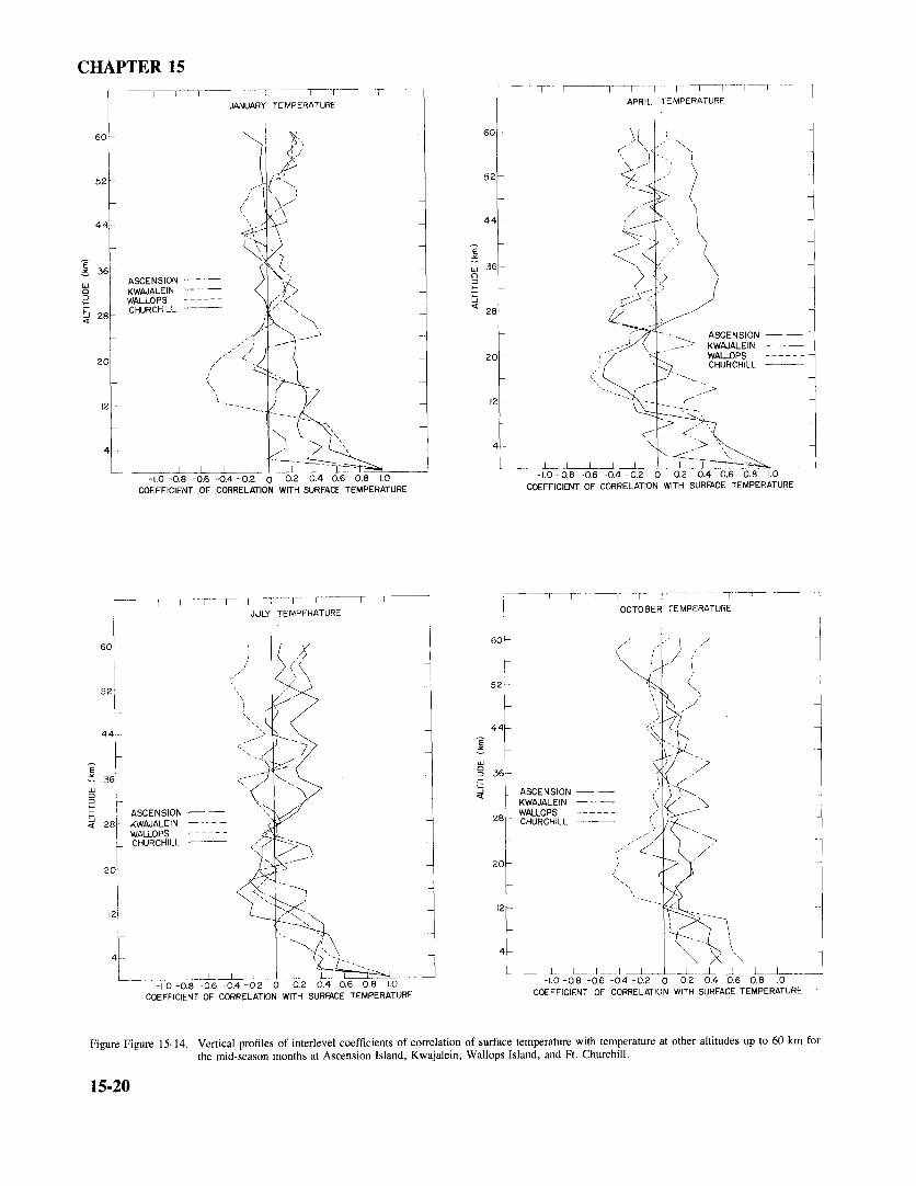
the monthly means. The standard deviations of observed between the levels is an example of the general problem oftemperatures around the mean monthly values for the mid- correlation decay. Correlation decay is similar for most me-season months at Ascension Island, Table 15-9, are typical teorological elements as the horizontal or vertical distanceof the day-to-day variations found in the tropics. Values are between the points of observations increases. As yet, nonot given for altitudes above 50 km as there are too few fully satisfactory description of the decay rate, based ondaily observations on which to base the monthly temperature fundamental properties or assumptions, is available. Con-distributions. The observed standard deviations includes the sequently, many empirical models that are valid for specificrms instrumentation errors as well as the actual rms climatic elements over restrictive ranges have been proposed.variations. Consequently, the observed variations are some- Profiles of correlation coefficient r, of surface temper-what larger than the actual values. ature with temperature at other altitudes are shown in Figure

Day-to-day variations of temperature around the annual 15-14 for the midseason months at Ascension Island, Kwa-mean at levels between 50 and 90 km in tropical areas (Table jalein, Wallops Island, and Ft. Churchill. At most locations,15-10) were computed from data derived from grenade and the correlation between surface temperatures and tempera-pressure-gage experiments at Natal, 6°S, and Ascension tures at other altitudes decreases rapidly with increasingIsland, 8°S. These data were not uniformly distributed with altitudes, reaching a minimum or becoming negative be-respect to season or time of day. An analysis of the relatively tween 12 and 16 km and then remaining near zero, plus orsparse data that are available for individual months indicates minus 0.3, from 20 to 60 km. Individual arrays of the meanthat if the seasonal and diurnal variations are removed from temperatures, standard deviations and interlevel correlationthe data, standard deviations around monthly means due to coefficients for altitudes to 60 km are given in Table 15-day-to-day changes in synoptic conditions would be roughly 12a to 15-12f for the months of January and July at Ft.50% of those given in Table 15-10. Churchill, Wallops Island, and Kwajalein. Additional in-

Table 15-10. Standard deviations of observed densities (%) and temperatures (K) around the mean annual values of Ascension Island (8°S)/Natal (6°S).

Altitude Density Temperature(km) S.D. (% of mean) S.D. (K) No. of Observations

50 4.1 6 3355 4.3 3 3360 4.8 6 3365 4.7 7 3370 6.4 9 3275 8.6 10 3180 7.8 10 3085 10.2 13 2990 12.3 21 28

15-18

ATMOSPHERIC TEMPERATURES, DENSITY, AND PRESSURE

Table 15-11. Mean temperature and standard deviation at standard pressure levels over North America.

Mean Temperature and Standard Deviation (K)

Pressure 20°N 30°N 40°N 50°N 60°N 70°N 80°N(mb) Mean S.D. Mean S.D. Mean S.D. Mean S.D. Mean S.D. Mean S.D. Mean S.D.

January

700 280 2 275 5 267 6 256 8 251 8 247 7 245 6500 264 3 259 4 252 6 242 7 238 7 234 5 232 5300 236 3 232 3 227 4 221 4 220 4 217 4 214 5200 217 3 216 5 216 6 219 7 219 7 216 6 213 6100 198 3 204 4 212 4 218 -5 219 6 216 7 210 650 208 3 209 3 213 3 215 4 216 * 213 * 206 *25 218 2 218 3 216 4 212 5 212 * 208 * 203 *15 225 2 223 3 221 4 218 6 215 * 211 * 207 *10 230 2 227 3 224 4 221 -6 217 * 213 * 209 *

July

700 283 2 283 2 282 3 275 4 270 3 268 4 265 4500 267 2 267 2 264 3 258 4 255 4 253 4 249 4300 240 2 240 2 237 3 232 4 229 4 228 4 227 4200 218 2 218 2 219 3 221 5 224 5 226 5 230 4100 200 3 203 3 210 3 220 4 226 3 228 2 231 250 213 2 215 2 218 3 221 3 226 3 228 3 230 325 222 2 222 2 225 2 227 2 229 2 232 2 233 215 228 2 228 2 229 2 232 2 235 3 236 3 236 310 232 2 233 2 234 2 237 2 239 3 240 3 241 3

*Not normally distributed.

formation useful in design studies is given by Cole and considerable variability produced by small-scale terrain fea-Kantor [1980]. tures, differences in soil moisture and cultivation. A snow

surface is markedly affected by aging. The physical con-ditions of water in a shallow puddle are quite different from

15.1.4 Speed of Sound vs Temperature the open ocean. All these conditions reflect themselves inthe micro-climatological aspects of natural or unnatural sur-faces.The speed of sound is primarily a function of temper- As discussed in Section 15.1.2, the use of ordinary

ature. An equation for computing the speed of sound and thermometers to measure surface temperature, will result inthe limitations of such computations are presented in Chap-

meaningful values only in the rare cases of a flat, uniform,ter 14. Figure 15-15 shows the relationship between tem and homogeneous surface. In general, area averages of tem-perature and the speed of sound. It can be used with the perature obtained by an integrating method over certainvarious temperature presentations given in this section to defined sections will be more representative than any oneestimate the probable speed of sound for various altitudes of a multitude of widely varying point values. Bolometric

and geographical areas. temperature measurements from an airplane cruising at low

altitude provide a more reasonable approach to the problemof surface temperature determination than a series of ther-

15.1.5 Earth/Air Interface Temperatures mometric point measurements. Table 15-13 lists some re-sults of bolometric measurements from an airplane. The data

The earth/air interface is either a land, snow, or water illustrate the great horizontal variability of surface temper-surface. At many locations, the physical structure of the ature even when effects on the scale of less than 6 m linearinterface is overwhelmingly complex. The land surface can dimension are averaged out.be covered with seasonally varying vegetation of great di- The processes that determine the temperature of theversity, and even without plant cover there is normally a earth/air interface and the surface characteristics that influ-

15-19

CHAPTER 15

JANUARY TEMPERATURE APRIL TEMPERATURE

60 60

<1,'' 6./ >52 - 52

44 - 44-

_~~~~~~~, .- :e -IS

36 36ASCENSION----

- KWAJALEIN . i

WALLOPS -- ,-./

28 - CHURCHILL - 28

.--- - ASCENSION - -,./,, - ,~~~~-jX/ ~~ .... ~~-~ ~ ~KWAJALEIN -- -

~20 o ~ . 20 '- WALLOPS -------~~~~~~~~~~~~20 _-~~~~~~~~~~~ .' _ _ ~,'CHURCHILL

12 _ ---- _12 - --- .

4 _ . > 4-

-1.0 -_8 -0,6 -04 -0.2 0 0.2 0.4 0.6 0.8 1.0 -I10 -08 -0,6 -0.4 -02 0 0.2 0.4 0.6 0.8 1.0

COEFFICIENT OF CORRELATION WITH SURFACE TEMPERATURE COEFFICIENT OF CORRELATION WITH SURFACE TEMPERATURE

-r~~~ - I--1 -I I -- Ir- --T- T -X-

JULY TEMPERATURE OCTOBER TEMPERATURE

60 "/60

52 52-

44 44 -

E~~~~~~~~~~~~~~~~~~~~~

Zf 36 36 IUJ~~~~~~~~~~~~~~~~~~~~~~~~~~~~~~~I

Dt~ 36 < ._> W _ C] 36 _ ~~~~~ASCENSION --KWAJALEIN -,1//-

I ASCENSION - 28 WALLOPS ------<z 28 KWAJALEIN CHURCHILL

WALLOPS ------

2 CHURCHILL -S X--2 ,g w

Y a/)~~~~~~~~~~/20 220

12 ~~~~~~~~~~~~~~~~~~~~~~~~~~~~12-

4~~~~~~~~~~~~~~~~~~~~~4- t'/b - I

-I 0 -0.8 -0.6 -0.4 -0.2 0 0.2 0.4 0.6 0.8 1.0 -10 -0.8 -0.6 -0.4 -0.2 0.2 0.4 0.6 08

COEFFICIENT OF CORRELATION WITH SURFACE TEMPERATURE COEFFICIENT OF CORRELATION WITH SURFACE TEMPERATURE

Figure Figure 15-14. Vertical profiles of interlevel coefficients of correlation of surface temperature with temperature at other altitudes up to 60 km for

the mid-season months at Ascension Island, Kwajalein, Wallops Island, and Ft. Churchill.

15-20

ATMOSPHERIC TEMPERATURES, DENSITY, AND PRESSURE

ence these processes may be separated into the following perature is shading. Thin roofs (metal, canvas), however,four classes: may attain a temperature so high that the under surface acts

1. radiative energy transformation (or net radiation in- as an intense radiator of long-wavelength radiation, thustensity), which depends upon the albedo and selective ab- acting to warm the ground. In hot climates, multilayer shadessorption and emission; with natural or forced ventilation in the intermediate space,

2. turbulent heat transfer into the air (by both convective or active cooling of the outer surface by water sprinkling,and mechanical air turbulence); can be used to cool the ground with some success. Table

3. conduction of heat into or out of the ground, which 15-15 compares temperature measurements of various ma-depends upon the thermal admittance of the soil; and terial surfaces with corresponding air and soil temperatures.

4. transformation of radiant energy into latent heat byevaporation, which depends upon the dampness of the sur-face or available soil moisture at the ground level.

The aerodynamic roughness of a natural surface strongly 15.1.6 Subsoil Temperaturesinfluences the momentum exchange between ground and airflowing past it. The momentum exchange establishes the The thermal reaction of the soil to the daily and seasonallow-level profile of mean wind speed. The mechanical tur- variations due to the earth's rotation and its revolution aboutbulence produced by surface roughness also determines to the sun of net radiation is governed by the molecular thermala certain degree the relative amount of heat transported into conductivity of the soil, k, and by the volumetric heat ca-or from the air at mean ground level. Other conditions being pacity of the soil, C = pc (where p is the density and c isequal, an increase in roughness and hence mechanical tur- the heat capacity per unit mass). For a cyclic forcing func-bulence will cause lowering of maximum surface temper- tion of frequency n, the quotient (nk/C)1/2 (which has theature during daytime and raising of minimum surface tem- physical units of velocity) determines the downward prop-perature during nighttime. For ordinary sandy soil, under agation or amplitude decrement with depth of the soil-tem-average conditions of overall airflow and net radiation on perature response. The product (nk C)-1/2 , which has thesummer days in temperate zones, the diurnal range of sur- physical units of degrees divided by Langleys per unit timeface temperature is about 17 K if the roughness coefficient (1 L/s equals 4.186 x l0 4 W/m2), governs the amplitudeis 0.06 mm or 14 K if it is 6.35 mm (roughness coefficient, of the temperature profile in time at the soil surface. Thealso called roughness "length," is E/30 where E is the av- ratio k/C is the thermal diffusivity (physical units of lengtherage height of surface irregularities). squared per unit time). The expression (kC)1/2 defines ther-

A special and rather extreme case of the influence of mal admittance of the soil.surface characteristics is represented by forests. The trees The continuous flow of heat from the earth's hot, deepintercept solar radiation and the heat absorbed is given off interior to the surface is the order of 10-5 L/min. This isinto the air that is trapped between the stems. Although deep very small compared with a solar constant of 2 L/min,snow may lie on the ground, daytime temperatures in wooded average net-radiation rates of 0.2 L/min, and induced soil-areas in spring can reach 289 K. heat fluxes in the uppermost several feet of the earth's crust

The thermal admittance (Section 15.1.6) of most soils of 0.1 L/min. Only for depth intervals in excess of aboutdepends on porosity and moisture content. Because both the 30 m must the heat flow from the earth's interior be con-thermal conductivity and heat capacity of soils increase with sidered, inasmuch as it results in vertical temperature gra-soil moisture, the thermal admittance may be significantly dients of the order of 2.5 to 25 K/km.affected by humidity variations during rainy or wet weather Table 15-16 gives experimental data on thermal admit-periods, whereas the normal diffusivity may remain unal- tance and theoretical values of the half-amplitude depthtered. These effects are difficult to assess, however, because interval based on experimental thermal diffusivity data forthe dampness of the surface is also a major factor in the diverse ground types. The smaller the thermal admittance,utilization of solar energy for evaporation. If soil moisture the larger the surface-temperature amplitude for a givenis readily available at the earth's surface, part of the net forcing function. This latter inverse proportionality is validradiation that would have been used for heating air and only when turbulent heat transfer into the atmosphere isground is used instead for latent heat of evaporation. Table negligible.15-14 lists observed temperatures in the air and soil at levels In a simple theoretical model of thermal diffusion, anclose to the earth/air interface. effective atmospheric thermal conductivity K is introduced.

Engineers must consider the effect of albedo and color For air, K is many times larger than the molecular thermalor net radiation in artificially changing surface or ground conductivity of the air. For the same forcing function, thetemperature. In India, a very thin layer of white powdered surface-temperature amplitudes at two different kinds oflime dusted over a test surface made ground temperatures ground follow the ratioup to 15 K cooler; the effect was felt at a depth of at least20 cm. (TAR)2 + (K/k)}12 2

1,2 ~~(15.21)Another effective method of controlling surface tem- (TAR), + (K/k) 2 (15.1)

15-21

Table 15-12a. Ft. Churchill-Correlation of January temperatures (K) from surface to 60 km.

KM Kilometers above Sea Level

MEAN Average of Observed ValuesSTDV Standard Deviation of Values Times 10N Number of Values at Each Altitude

KM .0135 2 4 6 8 10 12 14 16 18 20 22 24 26 28 30 32 34 36 38 40 42 44 46 48 50 52 54 56 58 611

MEAN 244 25(0 24(0 228 219 219 219 218 218 217 219 218 219 217 218 219 223 225 230 233 238 243 248 252 255 258 258 259 257 257 258

ST()V 75 58 49 43 45 52 61 70 75 78 63 69 70 98 96 88 85 89 109 125 166 171 187 173 160 148 143 147 146 138 127N 51 51) 511 5( 51) 50 50 50 46 40 30 29 23 45 48 50 5I 5I 51 5I 5I 5I 51 5I 51 5I 5I 51 49 46 36

2 72 `4 5 3 84

6 5 5 75 82

8 46 23 17 47

III 301 3 -4 1 3 85

1 2 321 1 6 9 1 9 73 941 4 34 2 1 1 2 2 3 68 89 981 6 25 189 I I 1 7 56 8 1 94 981 8 26 2 3 1 3 III 45 7 1 85 90 95

21) 22 1 4 8 I 3 8 6 1 73 7 8 8 3 94

22 24 1 4 1 7 4 310 5 59 59 65 80 93

24 2 2 1 6 2- 5 9 28 33 28 40 62 84 9826 6 - I 1 - I 1 7 44 55 5 8 66 76 80 94 96

28 1 I 7 I 9 33 45 48 62 74 79 92 94 96

301 -I1 4 1 4 III 4 1 9 29 33 5 3 66 7 2 86 8 3 87 95

3 2 - I - 3 II -I - 22 - 17 - 13 - 13 7 1 9 39 59 7 1 56 7 3 8434 -I I I 2 1 8 - 23 - 29 - 29 -29 -IS5 -5 1 8 3 7 50 32 51) 64 88

36 -6 I 16( 4 - 24 - 35 -37 - 37 -31 - 19 1 8 31) 34 1 2 29 44 74 853 8 5 I 8 -2 - 18 - 28 - 34 -35 -30 -17 9 IS5 2 1 - I 1 3 2 7 60 7 8 92

411 1 3 6 6 -2 - 14 - 27 - 34 -37 - 37 -29 - 3 0 6 - 19 -III I 3 7 6 1 78 92

4 2 9 I 4 2~ -IS - 32 -42 - 46 -50 -46 - 16 - 16 - 10 -39 - 29 - 16 26 5 1 70 84 9344 7 - I - I -8 - 22 - 39 -49 -52 -59 -55 - 33 -35 -23 -53 - 46 - 36 3 34 55 72 82 9246 II - 6 -6 - 15 - 30 - 44 - 53 - 56 - 63 -59 - 36 -39 -32 -52 - 47 -41 -3 25 46 60 74 83 93

48 -l I II - 10 - 21 - 33 -47 - 58 -61 -65 -62 - 42 -41 -35 -52 - 46 -41 -3 24 43 55 67 7 8 89 96

5(0 -I -II -17 -29 - 33 -44 - 52 - 53 -57 -52 - 36 -36 -35 -45 - 42 -40 - 14 II1 27 39 5 2 59 73 8 1 87

52- -3 -13 - 21 -31 - 29 - 37 - 44 -44 -48 -50 - 32 -34 -35 -43 --43 -46 -22 - I 1 3 22 36 44 59 68 76 9254 -5 -1 2 -21) -3(1 - 25 -31 -37 - 37 -43 - 5I - 41 -46 -46 -47 - 49 -54 -34 - 13 I 8 22 3 2 47 56 63 79 93

56 --59 -14 -22 -32 - 23 - 23 -26 -25 -33 -41 -41 -45 -44 -34 - 38 - 49 -41 - 24 - 14 -7 4 13 28 36 47 67 81 92

58 -4 -14 -201 -28 - 16 -IS5 - 17 -I -521 -36 - 43 -46 -49 -28 - 33 -45 -45 - 34 - 31 -27 - 20 -9 10 18 34 59 74 85 95

611 -211 -23 - 24 - 36 - 18 - 14 - 19 - 17 -24 -31 - 49 -SI1 -50 -38 - 38 -49 -44 -40 - 32 -27 - 22 -5 12 22 32 50 61 75 81 87

**Multiply tabular values by 0.01 to obtain correlation coeffecients.

Table 15-12b. Ft. Churchill-Correlation of July temperatures (K)from surface to 60 kin.

KM Kilometers Above Sea LevelMEAN Average of Observed ValuesSTDV Standard Deviation of Values Times 10N Number of Values at Each A~itude

KM .035 2 4 6 8 10 12 14 16 18 20 22 24 26 28: 30 32 34 36 38 40 ,42 44 46 48 50 52 54 56 58 60MEAN 284 277 265 252 23~ 228 224 225 225 225 226 227 229 231 235 238 242 247 252 257 262 268 274 278 279 280 278 276 274 271 269STDV 53 37 40 47 49 25 49 22 23 22 '20 18 I6 24 21 25 24 32 30 30 35 37 34 31 39 41 43 45 39 38, 43N 28 28 28 28 28 28 28 28 28 28 28 27 27 28 28 28 28 28 28 28 28 28 28 28 28 28 26 25 25 21 20

2 49 **4 53 89

-I~]6 49 87 95g 44 82 90 96

10 19 35 42 42 55

12 Z4 -66 -69 -76 -73 -3t4 22 -69 -73 -74 -74 -12 83

16 36 - 82 - 84 -84 - 82 - 32 69 78 [~18 -22 -75 ~71 -69 -66 -33 -46 ~63 -90

20 15 -66 56 -52 J50 -28 27 45 72. 91 .[~

22 13 -71 -65 -61 '-59 36 43 5'4 81 93 97 ~]24 13 -65 -61 -53 -54 -37 37 52 76 80 81 8526 I 37 -39 -37 -39 -18 27 42 54 53 48 55 6228 I -32 -36 -37 -33 -6 29 44 50 48 38 44 49 92

30 19 -20 - t6 15 - 19 - 14 19 27 34 25 14 25 37 82 77

32 26 -9 -I7 -II -12 -12 15' 33 28 27 16 27 31 78 76 '8234 41 -4 - I0 - 11 - 12 =6 22 27 26 24 9 21 17 64 67 78 8436 22 20 - 21 - 23 24 - 6 32 32 28 17 4 14 27 56 54 71 62 72 ~m]38 1.9 -23 -28 -33 =33 13 17 29 32 25 17 23 '23 68 73 66 63 64 6640 '~

30 -8 - 18 -21 -:19 -8 5 12 34 41 34 35 32 68 70 58 56 63 49 69

42 39 15 7 I 2 I0 6 5 17 '17. 7 II 6 52 63 57 60 64 38 54 7744 23 II -I -6 I 7 18 9 17 11 - 6 4 0 45 54 46 51 -59 47 44 -62 8046 15 - 10 - 8 ~ 18' - 16 - 7 9 w I 16 15 4 6 2 47 50 41 38 5t 55 61 51 42 6148 29 15 13 12 12 I0 0 -I0 0 1' 9 - 7 0 37 40 38 48 55 51 41 45 38 52 71

~[~50 40 25 23 26 20 14 4 4 -6 - 10 -22 - 18 0 37 34 49 63 60 57 38 33 38 53 45 8052 r~

20 9 3 5 I 9 22 26 15 -5 - 27 - 19 3 42 42 59 70 58 54 40 25 47 56 40 64 9054 2 - 8 -I1 -9 -'12 9 27 37 31 12 - 9 -t l0 46 51 55 67 54 52 47 26 50 53 49 65 78 9356 12 7 -12 7 -9 4 24 34 29 I1 -13 3 8 43 51 57 69 64 57 54 34 54 63 52 68 81 91 9558 6 -25 -t6 6 8 6 11 39 44 35 22 24 38 57 59 61 72 67 43 52 43 46 49 37 55 71 80 87 93

60 9 -9 4 6 7 19 2 14 29 19 5 7 26 50 58 54 55 58 36 48 41 47 $6 46 60 66 69 77 81 90

**Multiply tabular values by 0.01 to obtain correlation coefficients

C3

Table 15-12c. Wallops Island Correlation of January temperatures (K) from surface to 60 kin.

KM Kilometer above Sea LevelMEAN Average of Observed ValuesSTDV Standard Deviation of Values Times 10N Number of Values at Each Altitude

KM .015 2 4 6 8 I0 12 14 16 18 20 22 24 26 -28 30 32 34 36 38 40 42 :44 46 48 50 52 54 56 58 60MEAN 275 269 260 248 235 222 216 215 211 210 211 214 216 220 223 226 231 236 242 249 255 262 268 270 269 266 263 260 258 256 252STDV 54 86 79 69 53 33 55 39 44 45 35 35 38 45 54 59 60 63 6t 79 ~5 89 82 80 63 47 66 74 77 90 106N 44 44 44 44 44 44 44 44 43 43 43 43 43 44 44 44 44 44 44 44 44 44 44 44 44 44 44 44 40 34 19

2 74 **4 66 966 61 87 968 52 79 88 94

10 5 10 14 17 42

12 -44 -46 56 -62 -55 1314 -47 -65 73 -76 -74' -13 74

16 -54 -72 -78 -79 -79 -10 63 8918 -49 -79 82 -83 -81 -20 42 72 82

20 -41 -60' -59 -56 57 -14 28 51 58 72

22 -27 - 42 -41 -42 -48 17 .19 28 37 60 8124 -13 -32 28 -27 -3} -8 -1 2 12 34 52 64

26 7 -19 -19 -14 -18 -7 -2 -6 9 10 37 48 7328 0 t9 17 -15 -15 6 0 -3 -12 9 37 42 .60 86

30 11 -25 -22 -17 -I7 0 5 -4 -12 14 35 38 52 79 83

32 15 -19 18 ~15 -19 -1t -3 I -7 11 21 13 31 60 63 8234 t3 14 -19 -20 -23 -18 11 6 6 6 3 -9 8 30 29 55 8036 3 -15 -23 -29 -33 -30 15 8 7 11 -3 -13 -2 16 15 31 58 8138 -4 2 -5 -11 -7 -9 4 -10 -4 -3 -25 -36 -24 -22 -26 -26 -2 30 60

40 -10 I 5 -9 -2 .0 5 -13 -9 -10 -29 -42 ~29 -28 -32 -31 ~14 19 46 89

42 -12 5 5 9 14 8 -3 -28 -20 -27 -43 -44 ~23 ~29 -29 -30 -17 6 29 68 7944 -16 3 5 10 12 8 3 -28 -17 -26 -35 -37 -29 -21 ~21 -22 -6 3 26 54 63 8546 - 23 - I 3 7 9 10 - 2 -2t - 12 - 21 - 30 - 36 28 22 ,21 -'29 - 12 - 2 19 52 .63 74 8748 ~17 I 5 18 10 7 ~14 -18 -14 -23 -33 -43 w34 '21 -14 w22 2 2 19 42 49 62 69 85

50 -14 -7 -5 I ! 4 3 -2 4 - 10 -30 -38 -32 -21 -21 - 15 16 20 33 45 40 42 49 61 76

52 [5 10 9 13 16 3 -7 ~6 -5 -14 -37 47 -40 -23 -16 11 10 25 41 47 33 32 26 33 40 6654 20 II 10 11 15 6 -7 4 2 -9 -23 -34 -. 34 -- 10 -3 0 15 17 32 25 8 10 16 12 18 36 8056 23 8 5 8 I1 6 -12 -7 2 -5 -7 15 -26 -1 0 I 14 11 23 12 0 3 8 10 21 29 58 8258 23 23 22 24 28 21 -8 ~14 -9 -17 -19 20 -37 -15 -13 -14 t -5 7 2 -2 1 9 22 29 33 51 71 89

60 27 19 22 21 29 51 -3 -23 - ~9 29 - 18 -9 -35 I -4 -4 14 -5 10 13 7 3 20 32 35 43 38 59 77 95

**Multiply tabular Values by 0.01 to obtain correlation coefficients

AT

MO

SPHE

RIC

TE

MPE

RA

TU

RE

S, DE

NSIT

Y, A

ND

PRE

SSUR

E

en, en

rnC.

x '

r C0C

en, en

C-

C

en G

n xt

en q:

'lso

rl'' rr,,

ox

-x

r co

v r ~~~~~~~~~~~'C

- C

l

C

rl CC

C

- ocen8

r, R

r C

t

000 C

- 'dnee

en t-

:O0000~~~~~~~~~~~

C-

-enO

0eno0 e_

C-e;;n

C-

Cl

r., -'00

C FrI_<

Clt

°,Cl

C-C

ennR

en

0-CC

-

l q<

e, '0. en

en en

C°

en en

en en C

l j

en

e 'C

I lC

C

-CC

$

Cl°

, °,?

en R

-

Cl~

~ ~ ~ ~ ~ ~ ~ ~ ~ ~ ~~~~~~~~~~~~~~~~c

-CC

- 0C

C

- -

Cl00C

I

C

C00

C

l enorr,_r

r o

o )

FCO

x w

~~~~~~~~~~~~~~~~~~~~~~~~~~~~~~~~~~~~~~~~~~~~~~~~~~~~~~~~~~c-0'E

2 ennee

Enne

en ennee

en en<

nn enr4t

jO

l °o

s o

r tr

,,u

CC

CC

C

: 00

Cl

en 00

en x

ivC

ltoo o

x l

CC

C

tose]r nenenen

C:-l

l en

ennee en

enen-- en

trs

00~~

~~

~~

~~

~~

~~

~~

~~

~~

~

0x<0

r* lrl

rn R

l =

n en

C-

x en v0

en en

Cleene

en C

-C-C

-- C

- =

~~~~~ oI~

~ ri0C

C

C

-; enxC

0 enr

r° ir

|° °

1r

t0l%

oll~e

C-

r- voC

I -en

rncr v

--t-

joor >

vrC

en enr

-nneC

~en en

enner C

- '

_0C

e, _

_n0Ol

en

o z> IN

C--en

enen en

enenenen --

Cl~

~~

~~

leI en

0)~

~~~ 2

Ns l

r °c vIN

CC

s =

<sr

-C-

r0le C

-l

C

en enee

o C

en en

en

r l x

~~~~~ ~ ~

~~I I

I I

I I

I [

I I

I I

I IreeC

00C

e C

l C

C-C

-l en

000 C

-l C

l C

- xxl-

-cos orrrcct

-C.<

rtr¢ l -

-e ene

-1

Ir- C

l r

C l

CIle

n enlrlr

Cl~

~

~ ~

~ ~~~~~~~~~

I [

I I

II III

o ~ ~ ~

~ ~~¢

0)" ®

I

~ ~

~''¢~ ~

~ ~

°¢~':

0) I ~~~~~~~~~~~~~~~~~l.

sC

lO

z lt

o r

00e l

x l

CR

eC

en

rOC

-CenR

s

00 e n-

e -t

$nnee en

-xR

vst r

-ClglC

- -len

en C

ll~l

Cl

CIlIN

-en~

l C

l1C-2S

Table 1542e. Kwajalein~orrelation of January temperatures (K) from surface to 60 km.

KM Kilometers Above Sea LevelMEAN Average of Observed ValuesSTDV Standard Deviation of Values Times 10N N/~mber of Values at Each Altitude

KM .008 2 4 5 8 10 12 14 16 18 20 22 24 26 28 30 32 34 36 38 40 42 44 46 48 50 52 54 56 58 60MEAN 30I ' 288 279 267 255 241 224 208 195 192

'206 212 217 221 225 228 232 237 242 247 253 257 262 267 27t 272 272 271 268 265 263

STDV 14 13 13 13 14 14 15 16 15 46 28 26 23 30 27 30 36 36 37 42 42 38 42 48 63 64 51 41 44 49 58N 42 42 42 42 42 42 42 42 42 42 42 42 41 40 +1 42 42 42 42 42 42 42 42 42 42 42 42 42 41 38 34

2 - 3 **4 15 396 11 15 488 -I - 20 23 28

I0 - 2 8 47 43 70

12 5 13 44 52 48 8514 5 -4 22 43 60 71 8016 14 I0 -13 6 19 8 15 2818 6 3 16 -34 -41 -57 -52 -63 1

20 -23 -18 -12 0 4 I -9' -5 -21. I0

22 -13 3 -15 -27 -21 -21 -27 -34 -33 33 3724 -14 3 -12 7 5 -26 -21. 7 -19 16 3 3126 4 15 -I 18 2 -7 - 18 -15 8 11 -28 -I1 628 0 4 5 -9 I -12 -18 -21 4 17 -9- -3 15 51

30 3 -I 9 - 26 I -16 -- 29 - 19 I 25 - 6 - 6 - 8 50 53.

32 16 - 3 24 -13 0 -2 - 14 - 19 - 2 24 -I 6 I 28 32 3934 ' 20 19 -11 -25 -22 -23 -26 -29 43 29 -27 -20 -30 34 6 29 3936 I1 31 6: -17 -I0 -16 -27 -38 27 38 0 -I -25 19 19 29 37 4738 13 - 9 - 7 28 6 3 - I0 - 19 17 26 25 - 8 - 39 24 - I 30 26 57 54

40 I I - 32 -40 - 8 -12 - 19 - 28 19 2~ -16 2 2 23 8 t8 21 44 29 4742 -22 32 3 8 -7 -13 -18 -32 26 24. -4 -3 5 8 34 24 30 33 34 24 5144 -I 7 - 33 - 23 - 22 - 25 - 22 - 29 19 29 - 3 - 2 - 11 18 14 25 9' 51 15 43 54 64

46 7 -20 -22 -43 -I0 -24 -30 -19 -10 16 -6 -2 8 36 I 4-1 15 35 4 32 7 8 3748 25 -I0 -12 22 -3 -21 -21 -d6 26 23 -25 -26 4 32 32 33 38 58 28 49 33 35 42 53

50 27 8 8 - 7 - 7 - 9 - 12 - 22 26 11 - 26 - 43 - 33 20 21 32 32 48 43 48 30 36 39 17 63

52 9 20 13 4 -6 -6 -I1 - 22 18 18 5 - 31 - 32 6 27 33 21 49 45 55 24 35 32 6 53 7754 17 12 -9 -4 -8 -7 -26 -34- 15 13 2 I -24 3 14 7 II 39 42 38 31 24 30 I 44 54 6456 28 22 25 -9 2 -7 - 21 -27 4 21 -2 12 -8 7 14 31 20 29 32 30 36 25 26 19 35 29 46 5958 33 6 32 -16 -4- -12 -20 -31 I 26 -28 -I0 -17 26 25 30 13 23 27 19 16 3 I 16 31 39 48 47 65

60 21 16 10 -2 -7 -7 -t4 -24 t3 18 -21 -42 -17 19 14 9 2 32 28 23 11 4 5 2 29 50 64 58 32 71

**Multiply tabular values by 0.01 to obtain correlationcoefficients

Table 15-12f. Kwajalein~orrelation of July temperatures (K) from surface to 60 km.

KM Kilomete~ Above Sea LevelMEAN Average of Observed ValuesSTDV · Standard Deviation of Values Times l0N Number of Values at Each ARitude

KM .008 2 4 6 8 l0 12 14 16 18 20 22 24 26 28 30 32 34 36 38 40 42 44 46 48 50 52 54 56 58 60MEAN 301 286 278 266 254 239 222 206 198 203 210 215 219 222 227 230 233 237 241 248 254 259 262 265 266 268 268 265 261 257 253STDV 12 8 l0 12 14 17 16 17 17 24 17 15 20 20 21 34 31 43 42 55 34 35 37 50 48 49 58 69 65 69 61N 31 31 31 31 31 31 31 31 31 31 31 30 29 25 30 31 32 32 32 32 32 32 32 32 32 32 32 31 31 30 27

2 33 **4 38 726 23 66 788 2 49 44 52

I0 4 57 50 52 77

12 4 64 52 54 72 94 I,~14 22 66 48 57 38 52 6616 26 6 II 0 -39 -30 -20 918 7 -II -26 0 -7 -10 -5 7 -22

20 -14 -I 12 22 -7 -II -15 -20 -15 -37

22 32 -4 -6 12 34 -29 -12 20 40 9 1511~24 28 18 43 42 0 -6 -3 20 18 2 25 14

26 - 2 - 3 I 17 26 4 8, 31 7 36 -40 IO 9 ['~28 -7 35 12 25 33 23 24 45 9 6 -38 -20 -19 45

30 12 30 19 31 15 8 26 44 7 6 -15 13 -6 34 47

32 28 46 32 42 IO 24 27 52 5 17 - 24 19 22 46 39 5234 24 46 43 44 20 27 32 43 5 2 - I 23 5 40 28 42 74 ~i~36 6 32 24 40 23 32 .34 39 18 - 14 14 29 -IO 33 13 38 50 72 ~]38 - 2 23 29 34 31 20 23 25 7 4 - 7 I0 5 36 29 28 44 55 5340 24 16 18 37 29 19 20 44 II -6 - 10 24 34 37 38 36 46 39 38 52 ~1~42 29 14 17 30 16 2 14 39 26 32 - 29 33 49 37 I0 19 39 24 25 42 4944 I 27 24 31 20 31 40 33 2 17 - 23 2 23 25 6 26 42 27 27 33 9 4946 0 16 23 27 9 t5 23 23 I - 5 - 8 7 9 20 13 35 30 27 27 44 18 29 76 1~48 5 5 9 21 4 -4 I 18 22 0 -23 39 -18 53 20 39 32 43 54 44 36 36 36 6150 I -4 -8 17 13 3 5 12 12 24 -29 25 -21 60 29 21 19 23 32 21 15 24 33 46 7952 II - 22 -I 7 l0 7 6 6 -I 25 -29 0 -I 36 0 6 4 14 9 16 12 18 31 48 48 6454 21 -5 5 7 12 ~6 21 31 -II 33 -38 I 8 24 I 25 21 25 25 16 26 27 42 43 43 42 7656 17 I 2 II 17 22 24 35 - 19 33 -51 0 -2 36 25 27 27 18 15 18 41 30 47 42 53 55 59 I~7758 25 20 23 44 9 12 II 37 2 18 - 34 20 14 28 50 38 40 28 28 28 46 35 40 53 65 62 47 55 76~) 34 26 21 43 4 23 21 48 9 18 -22 21 20 24 44 34 36 24 37 22 38 36 43 46 43 50 46 59 72 89

· *Multiply tabular values by 0.01 to obtain correlation coefficients I~

CHAPTER 15

cillations" [Lettau, 1954b]. The best insulator is still air orany porous material with air-filled pores, such as feathery

300 -snow; materials such as leaf litter have similar insulating

properties [Geiger, 1957].280 Much information is available on soil-temperature vari-

ations in various climatic zones. Table 15-17 gives annualt: ~~~~~26o8~~~~ _ / _ and daily temperature cycles in different soil types. In ad-

dition to the type of ground, certain meteorological factors240 such as rainfall and melting snow have marked effects on

~-F~~~~~ / ~~~~~~~the soil temperature. Snow cover is a leading factor in pro-220 tecting the soil from severe frost. On one extreme occasion

with an air temperature of 255 K, the temperature was 272200 K under a 13 cm snow cover, whereas on bare soil it was

251 K.0 2 29 300 ,0 320, ,0 340, 350 The soil-temperature variations illustrated in Figure 15-

270 280 290 300 310 320 330 340 35016 were obtained at a station cleared of pine trees but in

SPEED OF SOUND (m /see) generally wooded country. Topsoil and brown sandy loamFigure 15-15. Speed of sound vs temperature (K). (0 to 0.6 m) changed to brown sand and gravel that varied

from medium (0.6 to 2 m), to coarse (2 to 4 m), and againto medium (4 to 18 m). The water level was at 15 m. The

where TAR represents the ratio of the thermal admittance figure illustrates the amplitude decrease and phase retar-of the ground to that of air. For diurnal cycles of net ra- dation of the annual cycle with depth. Amplitudes of weatherdiation, the ratio (K/k)air is the order of 104. disturbances with periods of several days, as illustrated by

The most extreme surface temperature oscillation occurs the temperature curve of the 0.75-m level, decrease withover feathery snow where the amplitude may reach ap- depth more rapidly than the annual amplitudes. Qualita-proximately four times that over still water or sandy soil, tively, this agrees with the theoretical prediction of an am-and is at least 100 times as large as that over the turbulent plitude decrement proportional to the square root of theocean. An amplitude ratio of about 3.5 can be expected for length of the period of oscillation. The actual half-amplitudesurface temperature over dry vs moist sand surfaces. The- depth interval of the annual cycle can be estimated fromoretically, the penetration of thermal "oscillations" into the Figure 15-16 as being nearly 3 m, which is much largersoil is inversely proportional to the frequency of the "os- than the depth inferred from experimental values of thermal

Table 15-13. Bolometric records of area (approximately 37 m2) surface temperature from an airplane cruising at approximately 370 m along a constant

flight path, April 1944 [condensed from Albrecht, 1952].

Surface Temperature (K) - Bolometric Data

StandardSun's Shelter Temp.

Elevation Sky at Airport Baltic Sand Down OpeningDay Hour (degree) Cover K Sea Beach Land City Woods in Woods

9 13 to 14 40.4 10/10 282 275 285 287 281 280 2811 110 to 20 - 1.6 1/10 283 275 280 275 276 276 27816 19 to 20 - 1.8 9/10 287 277 281 280 280 277 27520 05 to 06 0.5 1/10 275 278 271 267 272 270 26629 14 to 15 42.1 4/10 280 280 319 315 290 289 296

Wind Speed Clear Cutting Drym/s Woods in Woods Peat Swamp Pond

7 19 - 4/10 0.5 275 271 267 273 27420 20 - 2/10 1.5 273 272 269 273 27326 20 - 3/10 2.6 275 270 272 272 274

Albedo values as determined by Albrecht: 5% 8% 8% 7% 5%

15-28

ATMOSPHERIC TEMPERATURES, DENSITY, AND PRESSURE

Table 15-14. Temperature of the air 10 cm above, and of the soil 0.5 cm below, the earth/air interface measured by thermocouples [Davidson and Lettau,1957].

Temperature (K) at Mean Local Time

Condition 0400 0600 0800 1000 1200 1400 1600 1800 2000

*Air 287.7 289.8 296.0 300.7 303.7 304.7 305.0 301.9 297.5*Soil 290.6 290.9 296.0 304.1 308.6 309.2 306.8 302.3 298.5**Air 281.1 282.5 291.5 297.9 301.7 303.0 301.1 296.1 292.3**Soil 284.8 284.6 291.4 303.1 310.8 310.3 304.3 297.8 293.8

*Mean soil moisture in 0 to 10 cm layer 10% wet weight basis.**Mean soil moisture in 0 to 10 cm layer about 4% wet weight basis.

diffusivity. The discrepancy may be caused by seepage or to conserve on the air conditioning load, or to dissipate heatdownward migration of rain water and the accompanying generated by power cables. The determination of frost pen-advection or transfer of heat. This process could increase etration depths is usually the principal concern.the apparent or effective thermal diffusivity for annual soil-temperature variations by factors of 4 to 8 times the ex-perimental values obtained in soil of constant moisture. The 15.1.7 Degree-Day and Temperature-Winddata in Table 15-17 are more in line with experimental Combinationsfindings than the curves in Figure 15-16. The limitation ofTable 15-17 is that the data are for clearly defined and nearly A degree-day is a unit adopted to measure the departureideal soil types that are seldom matched by actual ground of the daily mean temperature from a given standard. In theconditions. United States the number of heating degree-days, on any

Factors that must be investigated and assessed for any one day, is the number of Fahrenheit degrees of the 24-hone set of soil-temperature observations are (1) type and mean temperature below 65°F (291 K). Cumulated, day bystate of compaction of the soil, (2) moisture content and day, over the heating season, the total number of degreeseepage of the soil during the test, (3) position of the water days becomes an index of heating fuel requirements. In suchtable during the test, (4) type and color of surface cover, cumulation, the days on which the mean temperature ex-(5) amount and nature of traffic over the site, and (6) local ceeds 65°F (291 K) are ignored. When the centigrade scaleclimatic conditions. is used, the base is usually 19°C (292 K). The United States

Subsoil temperature information is useful in computing Army Corps of Engineers computes "freezing-degree days"thermal stresses and loads. Some examples are the deter- as the departure of the daily mean temperature from 32°Fmination of the depth to which a structure should be buried (273 K), a negative departure when above 32°F (273 K).when proximity to natural isothermal conditions is desired The National Weather Service supplies "normal degree-days,"

both monthly and annual totals. A few examples of the 30-year annual normals are 9274(F°) for Fargo, N.D., 5634(F° )

Table 15-15. Comparison of air and soil temperature with surface tem- for Boston, Mass. and 108(F °) for Key West, Florida.peratures of materials exposed on a tropical island withnormal trade winds. Air and material surface temperatures The wind-chill concept was introduced in 1939 by theat 1.2 m above, soil temperature at 2.5 cm below, the earth/ famous antarctic explorer, Paul Siple, to measure the cool-air interface. Exposed surface area about 930 cm

2 [Draeger ing effect of low temperature and strong wind combined.and Lee, 1953]. The wind-chill index is the equivalent temperature, in a

Temperature (K) normal walk (1.9 m/s) in calm air, corresponding to thecombination of actual air temperature and windspeed. It can

Highest Average be related to the heat loss H from a nude body in the shade.Material Recorded Max. Min. H is given by

Air (I.2 m) 302 301 299Soil (2.5 cm) 307 307 299 H = (10 VV + 10.45 - V)(306 - Ta), (15.22)Wood 314 310 298Aluminum 313 309 298 where H is the heat loss in kilogram calories per squareGalvanized Iron 318 311 3 298 meter of body surface per hour, Ta is the air temperatureBlack Iron 324 315 298 (K), and V is the windspeed (m/s). Neutral skin temperatureConcrete Slab 310 307 298 is roughly 306 K. For windspeeds greater than 1.9 m/s the

Concrete ___Slab__310 __307__298 ~ wind-chill index (Two) in K is given closely by

15-29

CHAPTER 15Table 15-16. Physical thermal parameters of diverse ground types [Lettau, 1954b].

Half-Amplitude Depth IntervalAdmittance (theoretical)

AdmittanceRatio (TAR), Annual Cycle Diurnal Cycle

Ground Type Ground to Air (m) (m)

SOILS

Quartz sand,medium-fine dry 110 1.0 0.058% moisture 230 1.6 0.0822% moisture 360 1.5 0.08Sandy clay, 15% moisture 280 1.3 0.07Swamp land, 90% moisture 340 1.0 0.05

ROCKS

Basalt 350 1.8 0.09Sandstone 380 2.2 0.12Granite 440 2.5 0.13Concrete 440 2.3 0.12

SNOW, ICE, AND WATER

Feathery snow 10 0.67 0.04Packed snow 100 1.4 0.07Still water 280 0.82 0.04Ice 320 1.4 0.07Turbulent ocean 103 to 105 61 to 610 3 to 30

TwC = (306 - H/22). (15.23) not used, or needed, with wind speeds less than 6 km/h(2 m/s).

This formula gives only an approximation because of in- Extreme temperature-wind combinations are frequentlydividual body variations, incoming radiation, and other fac- important in thermal equilibrium design problems, requiringtors affecting heat loss from the body. The formula is not estimates of the maximum steady wind speeds likely to be

Table 15-17. Annual and daily temperature cycles. Annual values areaverages for the years 1939 through 1940 at Giessen, Ger- 300o 1 1 1 1 1 _

many [Kreutz, 1943]. Daily values are averages of clear 298 964 _95

weather, 10 through 12 August 1893, Finland, after Homen[Geiger, 1957]. 295

293

Temperature (K)290 \.

Annual Means Daily Means Y 288 '- //..

Swamp Sandy Granite S "- / ' '

Loam Sand Humus Land Heath Rock < 285 \. //Land He a t Ro c -. ..... ;.......'

Surface 282.1 282.3 283.1 289.6 298.0 297.6 . ,

1.0 m above 283.8 284.3 284.3 -_ _ -_ 280 --.- 2m278 -- -- \2m

0.6 m above - - - 284.5 287.0 293.4 Z8 _ 2

Surface 275 I-

Amplitude 283.5 283.7 284.4 283.4 290.0 283.2 273 I I i 1 , I I

OCT NOV DEC JAN FEB MAR APR MAY JUN JUL AUG SEP

Half-Amplitude Depth Interval (m)Figure 15-16. Variations of soil temperature at indicated depths; North

Depth 1. 8 1.6 1.4 0.05 0.08 0.15 Station, Brookhaven, Long Island, October 1954 throughSeptember 1955, [after Singer and Brown, 1956].

15-30

ATMOSPHERIC TEMPERATURES, DENSITY, AND PRESSURE

330 t I X l I } | 15.2 ATMOSPHERIC DENSITY*-RECOMMENDED IN MIL-STD-210B UP TO 90 KM

FOR WORLD WIDE DESIlGN CRITERIA320 - The density data discussed in this section are from direct

and indirect observations obtained from balloon-borne in-31- - strumentation for altitudes up to 30 km, and measurements

from rockets and instruments released from rockets for al-300 titudes between 30 and 90 km.

0290 -

* * · 15.2.1 Seasonal and Latitudinal Variations280 - -

FREEZING * The Reference Atmospheres presented in Chapter 14270 _ provide tables of mean monthly density-height profiles, sur-

* face to 90 km, for 15° intervals of latitude between the

260 _ _ equator and the North Pole. Densities at altitudes between10 and 90 km are highest during the months of June and

.2~~~~~~~~0~~~~ @July and lowest in December and January at locations north~~~~~~~~250 _~~- _ of 30° latitude. In tropical and subtropical areas seasonal

0 ~~~~~~~~~~~~variations are relatively small with highest densities at levels240 _ -above 30 km occurring in the spring and fall.

I-~ ~~ i|~~ ~ l l l lMean monthly density profiles, surface to 60 km, ob-

10 20 30 served during the midseason months at Ascension Island,8°S, 14°W, Wallops Island, 38°N, 75°W, and Ft. Churchill,

WINDSPEED (mps) 59°N, 94°W, are plotted in Figure 15-18. Densities areshown as percent departure from the U.S. Standard At-

Figure 15-17. Extremes of temperature in combination with windspeed. mosphere, 1976. The individual mean monthly profiles crossWindspeeds, in general, were observed 12 to 30 m above or converge near 8 km and between 22 and 26 km. Boththe surface. The 35 observations were taken over a 5-yearperiod at some 22 stations widely scattered in the United are levels of minimum density variability. The level near 8States. The envelope is for the recommended U.S. design km is considered an isopycnic level because mean monthlycriteria. densities depart from standard by no more than 1% or 2%

regardless of the geographical location or season. Between22 to 26 km, however, there is a marked seasonal variability,

encountered at various temperatures. Figure 15-17 was pre- even though there is very little longitudinal or latitudinalpared from 4 years of 6-hourly and 1 year of hourly data variability during individual months. Seasonal differencesfor 22 stations in the United States [Sissenwine and Court, in the density profiles at the same three locations are shown1951]. It shows maximum steady (5-min) wind speeds that in Figure 15-19. The minimum seasonal variability of theoccurred with temperatures in the range from 236 K to 319 mean monthly values, 1% to 2%, occurs at 8 km, and theK during this period. The stations used in this study were maximum seasonal variability occurs above 60 km. Theselected as representative of climatic areas in the United seasonal variations are largest at Ft. Churchill and are small-States, Mountainous stations were unrepresentative of gen- est at Ascension Island.erally operational areas and were not among those selected.Also, the high winds of hurricanes and tornadoes were omit-ted from the figure. 15.2.2. Day-to-Day Variations

The wind speeds of Figure 15-17 occurred at anemo-meter heights, usually at 12 to 30 m above ground level The density at a specific altitude may differ from theduring the years of observation. The wind speeds at the 3- seasonal or monthly mean at that altitude due to day-to-daym level are approximately 20% less and even 50% less for changes in the weather pattern. The distribution of observedthe extreme low temperature (less than 252 K). densities in January and July at the most climatically extreme

The combination of values of temperature and wind- locations for which data are available near 30° , 450, 60° andspeed, recommended for extreme U.S. thermal equilibrium 75°N are shown in Table 15-18a to 15-18d for altitudes updesign criteria, are shown by the envelope in Figure 15-17. to 80 km. Median, and high and low values that are equaledThis recommendation is not valid in mountainous areas or or more severe 1%, 10%, and 20% of the time are givenin Death Valley. For the latter the criteria are the same as as percent departures from the U.S. Standard Atmospherefor world-wide criteria, as plotted in Figure 15-17. at 5-km altitude increments. The 1% values for altitudes

15-31

CHAPTER 15

JANUARY DENSITYAPRIL DENSITY

60 / 60 -

52 52

44 44 -4

Z~~~~~~~~~~~~~~~~~ E

36- 36 //

" ~~~~ASCENSION - -- ASCENSIONWALLOPS WALLOPS

< 28- CHURCHILL CHURCHILL28 I28

20 20

12 -12 -

~_ _ __ ~ ~ J- -- I I _ _ _ _ I I _ _II_

-30 -20 -10 0 I0 20 30 -30 -20 -I0 0 ! 0 20 30

PERCENT DEPARTURE FROM 1976 STANDARD PERCENT DEPARTURE FROM 1976 STANDARD

JULY DENSITY OCTOBER DENSITY

60 60

52 52

44 - 44 -

36 - 36

PI ASCENSION A- -4

28 Ii WALLOPS . WALLOPSCHURCHILL 28 CHURCHILL

20 20

12 7 12-

4 4 L-30 -20 -IO 0 0 20 30 -30 -20 -I0 0 I 0 20 30

PERCENT DEPARTURE FROM 1976 STANDARD PERCENT DEPARTURE FROM 1976 STANDARD

Figure 15-18. Latitudinal differences in the density-altitude profiles for the mid-season months at Ascension Island, Wallops Island, and Ft. Churchill.

15-32

ATMOSPHERIC TEMPERATURES, DENSITY, AND PRESSUREI r - ] I-~ - -- '-T I I I -I I X · | I I' - ~ I - 'T-- -T -F

ASCENSION DENSITY CHURCHILL DENSITY

60 - . 60- I .

52 - 52

44 -/44

-30~~~~~~~~~ -20 -10 0;' -0 -0 -0 0 3P36 JAN /LO APRJULYOCT

28 - OT 28 JiAUPLRJULYI DOT----

? / ~~OCT....20 20

12 -12 -

4 - 4

-30 -20 -I0 0 I0 20 30 -30 -20 -I0 0 I0 20 30

PERCENT DEPARTURE FROM 1976 STANDARD PERCENT DEPARTURE FROM 1976 STANDARD

above 30 km are considered rough estimates as they are[V--7- -r T--f-----7 -T- ---- F- based on the tails of the distributions of observed values

WALLOPS DENSITY plotted on probability paper. Estimates above 60 km are,o _ 0I less reliable than those at lower levels because of the paucity

:\ ~~~ k ~~~of data and larger observational errors at the higher altitudes.a , i. ~ ~ ' In tropical regions the monthly density distributions are

!52 / nearly normal for altitudes up to 50 km. Consequently,/ } " ) - reasonable estimates of the distributions of density in the

44 - / tropics can be obtained from monthly means and standard)'~~~ ,i~deviations. Standard deviations of the observed densities

X6~ . f ,' 1 / ~~~~~~around the mean monthly values at Ascension, given in:36 ,,, 56 | ,' i / Table 15-19, are typical of the day-to-day variations found

HF~ _/ ~ (a ~ 0 -----AN in the tropics [Cole and Kantor, 1980].H5 I APR

<28 _ i/ JULYOCT...

2,o' , 15.2.3 Spatial Variation

' / XThe rate of decay of the correlation coefficient betweenr? )~~~~~~~~~12 ,,, < ~~densities at two points with increasing horizontal separation

is directly related to the scale of the major features of the4 _J/ weather patterns that are experienced at a specific latitude

-30| J. i .. ~ [ aand altitude. Figure 15-20 provides information on the decay-30 -20 -10 0 0 20 30 of density correlations with distance near 60°N for altitudes

PERCENT DEPARTURE FROM 1976 STANDARD up to 60 km. The decay in density correlations below 20

km are based on an interpretation of data from studies ofFigure 15-19. Seasonal differences in the density-altitude profiles at As- the spatial correlations of pressure, temperature, density and

cension Island, Wallops Island, and Ft. Churchill. wind at radiosonde levels at locations between 30° and 70°N

15-33

CHAPTER 15

Table 15-18a. Median, high, and low values of densities given as percentage departure from U.S. Standard Atmosphere 1976 for January and July at30'N.

Median 1% 10% 20% U.S. StdAltitude (% of . iDensity

(km) Std) High Low High Low Hgh Low (kg/m3 )

January

5 1 + ! -3 0 -2 0 -2 7.3643 110 + I +4 -3 +3 - I +2 0 4.135115 +7 + 15 - I + 12 +4 + 10 +5 1.947620 +3 +7 -2 +5 +1 +4 +2 8.8910- 225 2 +4 -6 +3 -4 + I -2 4.008430 -4 +2 - 10 -2 -8 -3 -6 1.841035 -3 +3 -12 0 -8 -1 -6 8.4634 - 340 - I +2 -10 + 1 -7 0 -5 3.995745 0 +8 - 10 +3 -7 +2 -5 1.966350 + I1 + 12 -8 +7 -4 +5 -2 1.026955 0 +9 -10 +5 -6 +3 -4 5.6810 - 460 -2 + 12 - 15 +5 -9 +2 -6 3.096865 4 +21 -25 + 13 - 13 +7 -6 1.632170 -5 + 16 -26 +9 -17 +6 -12 8.2828 - 575 -7 +21 -25 + 13 - 15 +8 - 10 3.992180 -4 +21 -22 + 15 - 13 +8 -7 1.8458

July

5 -3 0 -5 -1 -4 -2 -4 7.3643- 110 + I +3 - I +2 0 +2 0 4.135115 +16 +20 +11 +17 +13 +17 +14 1.947620 +-8 +11 +14 +10 +5 +9 +6 8.8910 - 225 +4 +9 0 +7 +2 +6 +3 4.008430 +3 +7 - I +5 + I +4 +2 1.841035 +6 +10 +2 +8 +3 +7 +4 8.4634 - 340 +9 + 15 +2 + 11 +5 + 10 +7 3.995745 +12 +19 +4 +14 +7 +13 +9 1.966350 +13 +23 +6 +17 +8 + 15 +10 1.026955 +11 +20 +2 +15 +5 +13 +7 5.6810 - 460 + 13 + 14 - I +21 +3 + 19 +7 3.096865 + 15 +43 -6 +38 0 +30 +6 1.632170 + 15 +32 -9 +23 + 1 +20 +8 8.2828 - 575 + 10 +24 - 11 +20 -6 + 15 + 1 3.992180 +6 +22 -15 +17 -6 +14 + 1 1.8458

latitude [Bertoni and Lund, 1964]. Information on the spatial 50 km, zero correlation is attained at more than twice thatcorrelations at altitudes above 20 km is from a study by distance, or 4450 km. This analysis indicates the presenceCole [1979]. In that paper, data from constant pressure maps of disturbances with wavelengths of roughly 18 500 km atfor 5.0, 2.0 and 0.4 mb levels were used together with 50 km, close to planetary wavelength number one at 60°N.nearly simultaneous rocket observations at several pairs of Information from Kantor and Cole 11979] on the correlationsstations near 60°N to determine the rates of decay of density between densities at points up to 370 km apart in tropicalcorrelation at levels between 30 and 55 km. As Figure 15- regions is provided in Table 15-20, for levels between 1020 indicates, the rate of decay in density correlation with and 60 km.distance decreases substantially with altitude. At 10 km, for The rms difference between the densities at two pointsexample, zero correlation is attained at about 2000 km at can be estimated by

15-34

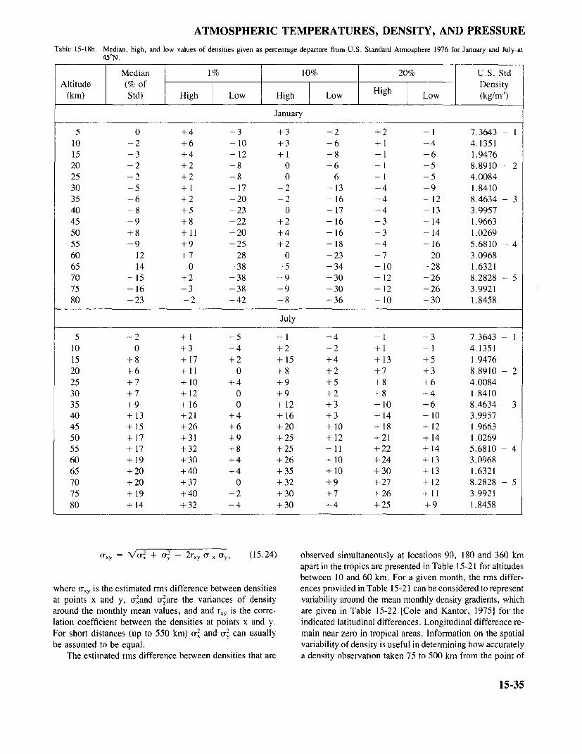
ATMOSPHERIC TEMPERATURES, DENSITY, AND PRESSURE

Table 15-18b. Median, high, and low values of densities given as percentage departure from U.S. Standard Atmosphere 1976 for January and July-at45°N.

Median 1% 10% 20% U.S. StdAltitude (% of Density

(km) Std) High Low High Low High Low (kg/m)

January

5 0 +4 -3 +3 -2 +2 -1 7.3643 - I10 -2 +6 - 10 +3 -6 + 1 -4 4.135115 -3 +4 -12 +1 -8 -1 -6 1.947620 -2 +2 -8 0 -6 - 1 -5 8.8910 - 225 -2 +2 -8 0 -6 - 1 -5 4.008430 -5 + I - 17 -2 - 13 -4 -9 1.841035 -6 +2 -20 -2 -16 -4 -12 8.4634 - 340 -8 +5 -23 0 - 17 -4 - 13 3.995745 -9 +8 -22 +2 - 16 -3 - 14 1.966350 +8 + 11 -20 +4 - 16 -3 - 14 1.026955 -9 +9 -25 +2 -18 -4 -16 5.6810 - 460 - 12 +7 -28 0 -23 -7 -20 3.096865 - 14 0 -38 -5 -34 - 10 -28 1.632170 - 15 +2 -38 -9 -30 - 12 -26 8.2828 - 575 - 16 -3 -38 -9 -30 - 12 -26 3.992180 -23 -2 -42 -8 -36 - 10 -30 1.8458

July

5 -2 +1 -5 - I -4 -1 I -3 7.3643- I10 0 +3 -4 +2 -2 + 1 - I 4.135115 +8 + 17 +2 + 15 +4 + 13 +5 1.947620 +6 +11 0 +8 +2 +7 +3 8.8910 -225 +7 + 10 +4 +9 +5 +8 +6 4.008430 +7 + 12 0 +9 +2 +8 +4 1.841035 +9 +16 0 +12 +3 +10 +6 8.4634 - 340 +13 +21 +4 +16 +3 +14 + 10 3.995745 + 15 +26 +6 +20 + 10 + 18 + 12 1.966350 + 17 +31 +9 +25 + 12 +21 + 14 1.026955 +17 +32 +8 +25 +11 +22 +14 5.6810 -460 + 19 +30 +4 +26 + 10 +24 + 13 3.096865 +20 +40 +4 +35 + 10 +30 + 13 1.632170 +20 +37 0 +32 +9 +27 +12 8.2828 - 575 + 19 + 40 -2 + 30 +7 +26 + 11 3.992180 + 14 +32 -4 +30 +4 +25 +9 1.8458

orxy = \/ r 2 + cry - 2ry or X oy, (15.24) observed simultaneously at locations 90, 180 and 360 kmapart in the tropics are presented in Table 15-21 for altitudesbetween 10 and 60 km. For a given month, the rms differ-

where Oxy is the estimated rms difference between densities ences provided in Table 15-21 can be considered to representat points x and y, or2and ro-2are the variances of density variability around the mean monthly density gradients, whicharound the monthly mean values, and and rxy is the corre- are given in Table 15-22 [Cole and Kantor, 1975] for thelation coefficient between the densities at points x and y. indicated latitudinal differences. Longitudinal difference re-

U2 .For short distances (up to 550 km) (rx and oy can usually main near zero in tropical areas. Information on the spatialbe assumed to be equal. variability of density is useful in determining how accurately

The estimated rms difference between densities that are a density observation taken 75 to 500 km from the point of

15-35

CHAPTER 15

Table 15-18c. Median, high, and low values of densities given as percentage departure from U.S. Standard Atmosphere 1976 for January and July at60°N.

Median 1% 10% 20% U.S. StdAltitude (% of Density

(kin) Std) High Low High Low High Low (kg/m)

January

5 +1 I +6 -3 +4 -I1 +2 0 7.3643 - 110 -6 +3 - 15 +2 -15 -3 - 10 4.135115 --9 -2 - 15 -5 -12 -6 - 11 1.947620 -8 -1 -155 - -11 -6 -10 8.8910 - 225 -7 +3 - 16 -2 -12 -4 - 10 4.008430 - 10 +7 -32 +2 - 18 -2 - 15 1.841035 -12 + 8 --35 -3 27 -3 - 19 8.4634 - 340 -15 + 10 -36 +5 -30 -4 -20 3.995745 -21 + 12 -39 +5 -34 - 10 -24 1.966350 -26 + 14 -43 +3 -36 - 15 -29 1.026955 -32 +9 -48 -10 -39 -20 -35 5.6810 - 460 -36 + 4 -54 -12 -40 -25 -39 3.096865 - 36 - 5 -50 -16 - 46 - 27 - 42 1.632170 -37 -12 -54 -25 -49 -32 -43 8.2828 - 575 --35 -- 10 -53 -24 -47 -30 -42 3.992180 -28 -11 -53 -17 -47 -21 -40 1.8458

July

5 --2 +2 -5 + I -4 0 -3 7.3643 - I10 0 +7 -8 +4 -5 +2 -3 4.135115 0 +6 -7 +3 -4 +2 -2 1.947620 +3 +7 -2 +6 0 +5 +1 8.8910 - 225 + 5 + 8 + I +7 +2 +6 +3 4.008430 +7 + 12 - I +9 +2 +8 +4 1.841035 -+ 10 +18 0 +14 +3 +12 +7 8.4634 - 340 +15 + 23 +5 +19 +10 +17 +12 3.995745 +20 +28 +7 +25 + 13 +23 + 16 1.966350 +25 +35 + 10 +30 + 16 +28 +22 1.026955 +27 +35 +11 +30 +16 +29 +22 5.6810 - 460 + 28 + 42 + 11 + 39 + 16 + 33 + 22 3.096865 +35 +50 + 11 +44 + 18 +39 +28 1.632170 +42 + 52 +12 +46 +20 +44 +30 8.2828 - 575 +44 + 58 + 12 +52 +20 +48 +35 3.992180 +40 + 56 + 10 +50 + 18 +44 +30 1.8458

vehicle reentry represents the conditions encountered in the surface to 60 km, together with interlevel correlation coef-reentry corridor. ficients between levels have been developed for tropical,

temperate and arctic regions [Cole and Kantor, 1980]. Ta-15.2.4 Statistical Applications to bles 15-23a to 15-23f contain statistical arrays of density

Reentry Problems for the months of January and July at Kwajalein (9°N),Wallops Island (38°N), and Ft. Churchill (59°N).

The relatively large number of available radiosondes and Variations in the range or deceleration of free fallingmeteorological rocket observations permit a detailed anal- objects or ballistic missiles that arise from day-to-day changesysis of the characteristics of atmosphere density profiles at in atmospheric density can be estimated from Tables 15-altitudes below 60 km. Arrays of means and standard de- 23a to 15-23f. The integrated effect, E, of mean monthlyviations of density at 2-km intervals of altitude from the density on the trajectory or impact point of a missile can

15-36

ATMOSPHERIC TEMPERATURES, DENSITY, AND PRESSURE

Table 15-18d. Median, high, and low values of densities given as percentage departure from U.S. Standard Atmosphere 1976 for January and July at75°N.

Median 1% 10% 20% U.S. StdAltitude (% of Density

(km) Std) High Low High Low High Low (kg/m 3)

January

5 +2 +6 -1 +5 0 +4 +1 7.3643 - 110 -8 +2 -18 -3 -13 -5 -10 4.135115 - 10 - I - 18 -6 - 14 -8 - 13 1.947620 -12 -1 -22 -6 -17 -8 -15 8.8910 - 225 - 15 -2 -28 -8 -20 - 10 -- 18 4.008430 -21 -4 -36 -9 -26 - 16 -- 24 1.841035 -25 0 -43 - 10 -32 - 16 -30 8.4634 - 340 -29 +4 -48 -9 -38 - 16 -- 38 3.995745 -33 +8 -52 -6 -45 - 16 -39 1.966350 - 38 +4 - 56 - 8 - 48 - 20 -42 1.026955 -44 +5 -65 -10 -56 -23 -50 5.6810 - 460 - 46 0 - 70 - 16 - 60 - 32 -55 3.096865 -47 + 1 -66 -27 -62 -35 -58 1.632170 -48 - I -69 -21 -62 -35 -60 8.2828 - 575 -45 - 10 -65 +25 -57 -35 -53 3.992180 - 40 - 8 - 55 - 24 - 50 - 34 - 45 1.8458

July

5 1 +4 -2 +3 -1 +2 0 7.3643 - 110 -4 +5 -12 +3 -- 10 0 -7 4.135115 -4 +2 -9 0 -7 -2 -6 1.947620 +1 +6 -4 +4 -2 +3 -1 8.8910 - 225 + I + 10 -8 +6 -3 +5 -2 4.008430 +7 + 13 +2 + 10 +5 +8 +6 1.841035 + 12 +25 +3 + 18 +8 +16 +10 8.4634 - 340 + 19 +27 +6 +23 + 13 +21 + 16 3.995745 +25 +35 + 10 +30 + 18 +28 +-21 1.966350 +27 +40 + 10 +35 +20 +32 + 24 1.026955 +32 +42 + 10 +39 +20 +35 +25 5.6810 - 460 + 37 3.096865 + 48 (Insufficient data above 55 km 1.632170 +60 in summer) 8.2828 - 575 +67 3.992180 +64 1.8458

be determined for a specific location by computer "flights" due to day-to-day variations from the mean seasonal or thethrough mean monthly or seasonal density profiles if the mean monthly density profile can be obtained fromproper influence coefficients, Ci, for the missle at variouslevels are given. For example, we can write trt= 'i, C o'i r i Cj %r, (15.26)

E = Cj (15.25) where r 2 is the integrated variance for all layers beingconsidered, Ci and Ci are influence coefficients at the ith

where pj is the mean monthly density at the ith level. The and jth levels, o, and cr are the standard deviations of densityinfluence coefficients depend upon aerodynamic character- at the two levels, and rji is the correlation coefficient betweenistics, reentry angle, and the speed of the vehicle. The densities at the two levels. In these computations density isintegrated standard deviation in range or deceleration Oint, assumed to have a Gaussian distribution at all levels. As a

15-37

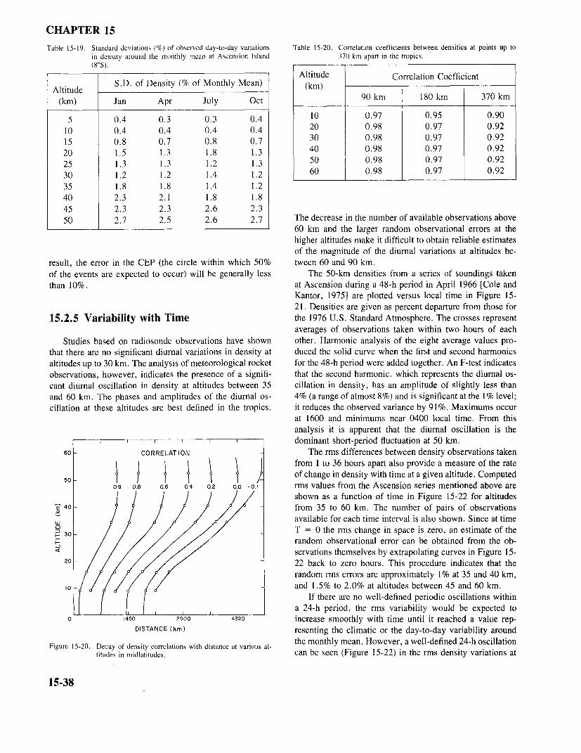
CHAPTER 15

Table 15-19. Standard deviations (%) of observed day-to-day variations Table 15-20. Correlation coefficients between densities at points up toin density around the monthly mean at Ascension Island 370 km apart in the tropics.(8°S).

Altitude Correlation Coefficient

Altitude S.D. of Density (% of Monthly Mean) (km)Altitude y(m(km) Jan Apr July Oct 90 km 180 km 370 km

5 0.4 0.3 0.3 0.4 10 0.97 0.95 0.9010 0.4 0.4 0.4 0.4 20 0.98 0.97 0.9215 0.8 0.7 0.8 0.7 30 0.98 0.97 0.9220 1.5 1.3 1.8 1.3 40 0.98 0.97 0.9225 I.3 1.3 1.2 1.3 50 0.98 0.97 0.9230 1.2 1.2 1.4 1.2 60 0.98 0.97 0.9235 1.8 1.8 1.4 1.240 2.3 2.1 1.8 1.845 2.3 2.3 2.6 2.350 2.7 2.5 2.6 2.7 The decrease in the number of available observations above

60 km and the larger random observational errors at thehigher altitudes make it difficult to obtain reliable estimatesof the magnitude of the diurnal variations at altitudes be-

result, the error in the CEP (the circle within which 50% tween 60 and 90 km.of the events are expected to occur) will be generally less The 50-km densities from a series of soundings takenthan 10%. at Ascension during a 48-h period in April 1966 [Cole and

Kantor, 1975] are plotted versus local time in Figure 15-21. Densities are given as percent departure from those for

15.2.5 Variability with Time the 1976 U.S. Standard Atmosphere. The crosses representaverages of observations taken within two hours of each

Studies based on radiosonde observations have shown other. Harmonic analysis of the eight average values pro-that there are no significant diurnal variations in density at duced the solid curve when the first and second harmonicsaltitudes up to 30 km. The analysis of meteorological rocket for the 48-h period were added together. An F-test indicatesobservations, however, indicates the presence of a signifi- that the second harmonic, which represents the diurnal os-cant diurnal oscillation in density at altitudes between 35 cillation in density, has an amplitude of slightly less thanand 60 km. The phases and amplitudes of the diurnal os- 4% (a range of almost 8%) and is significant at the 1% level;cillation at these altitudes are best defined in the tropics. it reduces the observed variance by 91%. Maximums occur

at 1600 and minimums near 0400 local time. From thisanalysis it is apparent that the diurnal oscillation is the

..... lt~ ~ l l l ldominant short-period fluctuation at 50 km.60 - CORRELATION The rms differences between density observations taken

w -t~~~ t t X tof change in density with time at a given altitude. Computed0.9 0.8 0.6 04 0.2 0.0 -o.1 rms values from the Ascension series mentioned above are

shown as a function of time in Figure 15-22 for altitudes40 from 35 to 60 km. The number of pairs of observations

available for each time interval is also shown. Since at timeF~.-~ 30 _ / / / / / // ~T = 0 the rms change in space is zero, an estimate of the30-

random observational error can be obtained from the ob-cr<~~~~~~~~ / / / / / //servations themselves by extrapolating curves in Figure 15-

20 22 back to zero hours. This procedure indicates that the

random rms errors are approximately 1% at 35 and 40 km,lo - J and 1.5% to 2.0% at altitudes between 45 and 60 km.

If there are no well-defined periodic oscillations withina 24-h period, the rms variability would be expected to

0 1450 2900 4320 increase smoothly with time until it reached a value rep-DISTANCE (km) resenting the climatic or the day-to-day variability around

Figure 15-20. Decay of density correlations with distance at various al- the monthly mean. However, a well-defined 24-h oscillationtitudes in midlatitudes. can be seen (Figure 15-22) in the rms density variations at

15-38

ATMOSPHERIC TEMPERATURES, DENSITY, AND PRESSURE

Table 15-21 Estimated rms differences (% of mean) between densities at locations 90, 180, and 360 km apart during the midseason months in the tropics.

January April July OctoberAltitude 90 180 360 90 180 360 90 180 360 90 180 360

(km) km km km km

10 0.10 0.13 0.18 0.10 0:13 0.18 0.10 0.13 0.18 0.10 0.13 0.1815 0.13 0.17 0.25 0.11 0.14 0.21 0.16 0.20 0.30 0.16 0.20 0.3018 0.50 0.61 1.00 0.34 0.42 0.68 0:30 0.37 0.60 0.34 0;42 0.6820 0.28 0.34 0.56 0.28 0.34 0.56 0.24 0.29 0.48 0.24 0.29 0.4825 0.28 0:34 0.56 0.28 0.34 0.56 0.24 0.29 0.48 0.26 0.32 0.5230 0.30 0.37 0.60 0.30 0.37 0.60 0.28 0.34 0.56 0.30 0.37 0.6035 0,34 0.42 0.68 0.30 0.37 0.60 0.30 0.37 0.60 0.36 0.44 0.7240 0.40 0.49 0.80 0.44 0.54 0.88 0.48 0.59 0.96 0.44 0.54 0.8845 0,46 0.56 0.92 0.40 0.49 0.80 0.60 0.73 1.20 0.52 0.64 1.0450 0.56 0.69 1.12 0.54 0.66 1.08 0.72 0.88 1.44 0.54 0.,6 1.0855 0;66 0.81 1.32 0.56 0.69 1.12 0.84 1.03 1.68 0.78 0.96 1.56

60 0.84 1.03 1.68 0.66 0.81 1.32 1.00 1:22 2.00 0.82 1.00 1.64

all altitudes between 40 and 60 km with maximums at 12 Unlike the tropics, a 24-h oscillation in density is not ap-and 36 hours and a minimum at 24 hours. An analyses of parent from this analysis which is based on eight years ofmeteorological rocket observations taken at Kwajalein (9°N) data at Ft. Churchill and ten years at Wallops Island. Theand Ft., Sherman (9°N) show similar results [Kantor and diurnal oscillation is relatively small and is probably maskedCole, 1981]. The diagram in Figure 15-22 and the results by instrumentation errors and changing synoptic patterns,of similar studies show that in the tropics an observation The rms variability at both locations increases with time24 hours old is more representative of actual conditions than until the climatic values of day-to-day variations around theone 12 hours old. monthly means are reached.

The observed rms variations of density with time lagsof 1, 2, 4 and 6 hours are shown in Figure 15-23 for levelsbetween 60 and 90 km at Kwajalein. This information, from 15.3 ATMOSPHERIC PRESSURECole et al. [1979], is based on a July 1978 series of high- UP TO 90 KMaltitude ROBIN falling sphere flights at Kwajalein. The firstprofile represents the estimated rms observational error. Pressure data provided in this section are based on (i)

The rms variations of density with time at the 50-km routine radiosonde observations taken by national weatherlevel are shown in Figure 15-24 for Wallops Island (38°N) services and extending to approximately 30 km, and (2)and Ft. Churchill (59°N) for the months of January and July. measurements from rockets and instruments released from

Table 15-22. Mean monthly latitudinal density gradients (% change per 180 km) in the tropics.

Altitude , January April July October(kin) Gradient (%) Gradient (%) Gradient (%) Gradient (%)

10 0.01 0.02 0.03 0.0415 0.15 0.17 0.08 0.0520 b.12 0.23 0.08 0.0625 0.04 0.14 0.10 0.1430 0.26 0.13 0.14 0.2135 0.13 0.22 0.16 0.2340 0.03 0.16 0.16 0.2045 0.14 0.01 0.17 0.2150 0.11 0.09 0.12 0.2055 0.08 0.12 0.04 0.i760 0.09 0.04 0.10 0.25

15-39

Table 15-23a. Kwajalein--Correlation of January density (kg/m) from surface to 60 km.

KM Kilometers Above Sea LevelMEAN AVerage of.Observed ValuesSTDV Standard Deviation of Values Times 10N Number of .Values at Each Altitude

KM .008. 2 4 6 8 10 t2 14: t6 18 20 22 24 26 28 30 32 34 36 38 40 42 44 46 48 50 52 54 56. 58 60*MEAN 1167 969 786 639 516 416 332 261 199 141 934 654 464 342 248 182 133 980 725 538 401, 303 230 175 234 105 818 640 504 397 310

-3 -3 3 3 -3 -3 -3 3 -3 -3 -4 -4 -4 -4 -4 -4 4 -5 -5- -5 -5 -5- '5 5 -5 -5 -6 -6 -6 6 -6STDV 15 5 4 4 5 4 5 5 10 28 15 13 12 48 15 15 t7 18 16 18

~21 20 23 28 22 28 28 33 34 37' 37

N 42 42 42 42 42 42 42 42' 42 42 42' 42 41 40 41 42 42 42 42 42 42 42 42 42 42 42 42 42 41 38 34

2 17 **4 17 376 4 7 228 -9 24 2 14

10 9- 10 17 9 58

.12 7 17 I 21 4-4~

7414 9 -9 - 23 3 23 27 49:16 2 7 -36 -II -7 -t0 4 2918 -3 2' - 22 -32 -37 -37 -14 -9 52

20 -t 9 8 19 7 28 17 7 12 t5

22 I 2 -22 -28. -25 I -4- 6 21 38 4224 -30 0. -12 16 -6

~-16 -5 27 14 7 5 31~

26 6 -4 6 -13 -4 4 -2 tl 31 15 -5 14 4128 16 14 tO 2 -14 9 I -9 23 3 9 t6 37 66

30 25 4 13 -14, -10 -8 -5 17 t7 4 6 8 21 64 67

32 15' -6 17 -14 -24 -- 8 -25 0 -4 . -2 7 10 14 30 39 5134 0 5 -21 -t0 -33 -8 -tl t0 27' -5 -2 -3 10 30 24 41 4836 8 21 -I 3' -32' 7 -t2 -2 7 -7 10 3 -6 3 18 31 35' 5238 10 -9 -3 12 3 33 16 16 -9 -18 32 0 -I 8 5 32 35 61 55 '

44t -I -16 - 24 7 -12 16 14 23 - 5 - 20 0 18- 36 t 8 14 24 45 36 57

42 4 14 4 34,-t4 7 11 17 -18 -30 6 l0 3t -12 24 15 27 33 39 42 7044 2 -3 -18 23 -20 8 12 29 -14 -23 9 t6 26 -2 13 19 21 49 34 59 72 8346 -5 15 -5 5 -6 4 3 31 -3t --26 6 16 32 3 4 22 22 31 19 44 47 58 7248 9 -20 - 12 19 -15 8 -3 29 -28 -30 -8 -4 34 - I 19 t4 33 39 26 42 45' 54 61 70

50 3 I 12 26 22 -3 -5 5 -32 -37 -4 - 1t 14 - I 22 25 34 37 52 44 56' 64 63 56 67

52 3 7 18 40 -17 5 15 9 -43 42 14' -I 5 -30 3 -I 7 18 40 35 45 64 62 58 58 8254 -2 -8 0 28 -16 0 0 6 -41 -43 9 15 5 -34 -14 -16 2 9 32 25' 52 60 63 62 53 67 8856 3 -5 24 26 - t4 -3 2 I1 -40 35 6 14 2 -31 -16 - 18 -3 7 19 14 42 56 55 62 41 52 79 9058 -9 -6 24 14 -19 5 0 12 -40 -28 7 27 4 -18 -II -20 0 -6' 20 14 35 50 55 67 43 62 81 88 92

60 -27 5 7 27 -20 6 I 7 -37 -29 4 14 4 -25 -20 -32 -I 6 38 14 29 49 51 5~ 45 64 83 67 80 91__

*Multiply mean by indicated :negative po.wer of 10.**Multiply tabular values by 0.01 to obtain Correlation coefficients

AT

MO

SPHE

RIC

TE

MPE

RA

TU

RE

S, DE

NSIT

Y, A

ND

PRE

SSUR

E

tm~ rI

frtrl

Cl

-l '0,0

rff ft

(r s

i ce

G ~ ~

~ ~

~ ~

~ ~

~ ~

~ ~

~ ~

O

00-ft ft

00 l

Cl

ft

-D

<

C

ftr

st t

I rr;

^ o~~~~~~~~~f ft

ft 0t

ft

Cl

oO

Cl

Cl

Cll

00 ftf

-C

g R

l

r 00

ft ftft00fX'00

i vB

|

r~~

q <

oo

8 °>

r

1~~

r-0

Of'

Cl

005~0

^0

f

000 fsf

ft ftt0f

00w

<r

.rlr s

00 l

C--

Of

Cl'00C

0

-'C

:~""~

~ ~

C

Cl

Cl

ZI

ClC

lC

f

]C

,

T

I

Cl 00

,

-i

,

Y

Cl.

ClQ

Q

j qqs

-ft

Cl

Cl

rll~~

C

l C

lo C

ls t

E

Clr l st

O-

r l

Co

o -

f

v Clo

00V

ClolCr

l ft<

.rz

-~'> ,

T,

0 ,

,

T: ~ T?

r , '

Doa

g ||g

r-

Cix l nC

R

rCrl

00C)

q l

.Crl

r- -°fi

°

H-

0C

lo O

R

Cl0CC

ft0Cr l$

r -s

Cl00

Cfi

Cl-Cft)

R

, ~:

Cllr

l C

°8o l

r vl t

xrl p

--

;

E~

~~

~~

~~

~~

~~

~~

I;

I

z rl

I

I

R

I

r° ! I

I

I

I

I

I~

x °

xt x

lort

r~~

~~

~~

~~

l~~

~

i' t ?l

o Iq I)

i I

I Io R

i

I '1 I

I I

I .l

so g

r~~

~~

~~

~~

~~

lftl C

n l

Cl00'00,

l f

r l tIfte03

s- ft

I I

I I

I I

I I

I I

I C

l ,

00CX

lst ~

r 00

0 O

- _

C

Cll0

CltstO

l d

00 Cl)

Vl

o rl

lf~

X

Cl

r

4, -

0Cf,00

0 _

-0°

HC

l C

ft

f O

f X

l -

X

f=

_i

ox o

lXox

Rr

'°l~C

~

00 R

l

Cl

00C

xltl t

00 00l40

C R

0

f r-4°t

15-41

46

Table 15-23c Wallops Island-Correlation of January density (kg/m) from surface to 60 km.

KM Kilometers Above Sea Level U~MEAN Average of Observed ValuesSTDV Standard Deviatiotvof V-alues Times 10N Number of Values at Each<Alitude

KM .015 2 4 6 8 10 12 14 16 18 20 22 24 26 28 30 32 34 36 48 .40 42 44 :46 48 50 5-2. 54 56 58 60'MEAN 1292 1029 821 *658 524 411 310 227 168 122 874 638 452 33 1 24! 175 128 936 689 509 379 285 216 187 130 102 601 627 486 378 2193

- 3 - 3 -3 - 3 - 3 -3 - 3 - 3 -3 -3 - 4 -4 - 4 -4 - 4 - 4 -4 -5 - 5 -5 -5 - 5 - 5 -5 -'5 -5 - 6 - 6 - 6 - 6 - 6STDV 23 26 16 10 IS 35 SI1 43 41 39 29 40 25 22 23 25 29 36 38 48 50 47 42 44 44 46 47 50 52 55 63N 44 44 44 44 44 44 44 44 43 43 43 43 43 42 43 43 43 43 43 43 43 43 43 43 43 43 43 43 39 33 16

2 74 -4 66 926 34 28 535 -29 -62 - 50 25

1 0 -33 - 75 - 74 -9 86

L2 -42 - 72 -79 -34 6 1 8414 -39 - 79 -83 - 31 60 84 9216 - 42 - 81 - 84 - 27 63 82 88 9718 - 39 - 82 -81 - 23 63 79 79 92 94

20 - 37 - 76 - 72 - 9 57 70 67 79 83 92

22 - 34 - 5I -47 -5 33 46 49 49 52 61 7224 - 21 - 53 -46 2 36 -39 40 48 55 69 76 5926 - 8 - 48 - 37 1 f 38 40 39 44 48 63 70 57 9028 - 21 - 50 - 41 5 45 45 35 41 43 58 62 SI1 79 83

30 - 13 -45 -37 II1 46 40 34 4! 43 55 53 41 65 73 8 1

32 - 12 -28 - 25 -3 2 1 18a 28 33 36 38 29 19 41 46 53 8034 - 17 - 18 - 24 - 21 9 7 25 23 24 .24 10 9 23 20 28 ~60 8636 - 27 - 17 - 25 - 32 3 I 23 22 25 20 4 I 14 4 1 2 38 69 8938 - 28 -89 - 16 - 32 - 5 - 8 9 6 9 3 -12 -12 -2 --16 - 13 9 42 7 1 87

40 - 29 - 8 -I14- - 23 - I - 8 6 3 6 0 -13 - 9 -2 --1g - 13 9 35 65 8 1 95

42 - 32 - 6 -7 -7 -6 - 16 - 3 - 5 0. -8 -18 I -3 --17 - 12 5 26 SI1 67 80 8744 - 34 - 7 -5 - I -6 - 13 I - 1 4 - 7 -16 3 - 12 -22 - 19 -2 1 9 *36 53 64 72 8946 -3( - 6 -2 3 -3 - 10 - 1 4 8 - 3-13 1 -12 -23 -19 - 1 3 30 45 57 66 79 9248 -21 - 6 -I., 4 - 1 -8 -2 7 9 - I -13 - I - 17 -22 - 19 -5 8 20 32 42 48 65 79 92

50 - 12 - 7 -5 -I I 0 .3 12 13 3 -12 I - 21 -23 -25 -7 I 12 18 24 28 42 60 75 91

52 -3 0 0 -3 -5 - 5 -2 7 7 - 3 -18 -10 - 29 - 31 - 30 - 13 - 8 9 15 19 20 34 48 .64 82 9454 - I 0 0 -6 -6 - 5 -3 7 8 - 3 - 16 - 14 - 30 - 32 - 35 - 21 - 19 - 8 0 3 5 .22 42 55 75 88 9456 I 6 6 -3 - 12 - 12 - 1I -I1 2 -6 - 16 - 17 - 28 - 29 -33 -22 - 23 -r5 - 9 - 8 -I1 13 33 SI1 74 86 87 9558 2 IS S1 4 -7 - 12 - 10 - 8 - 5 - 17 - 28 - 26 -39 -38 -40 -18 -IS5 - 5 I 4 13 27 44 61 78 88. 84 91 96

60 - 6 26 26 - 8 - 47 -46 - 32 -29 -23 -41 - 52 - 48 -SS -59 -69 - 55 - 39 -19 -3 10 '20 .43 59 7 1 83 92 87 91 93 98

*Multiply mean by indicated negative power of 10**Multiply tabular values by 0.01 to obtain correlation coefficients

AT

MO

SPHE

RIC

T

EM

PER

AT

UR

ES,

DE

NSIT

Y, A

ND

PRE

SSUR

E

00- ~~~~~~~~0

h-C

'0~~~~~ 1

I

z~~~~~~~~~~~~~~ >

21 C

Cll

l, 0

~~~~~~~~1-43'* Cl 00 C

f V

l C

l C

I 1

e. ~ ~

C

Cl

lC

00 0

Cl Cl

CC

~~~~I Cl

00I

zll ll

000 0

00~~~~~~~~~~~~~~~~~54

Table 15-23e. Ft. Churchill-Correlation of January density (kg/m) from surface to 60 km.

KM Kilometers Above Sea Level 3MEAN Average of Observed ValuesSTDV Standard Deviation of Values Times 10N Number of Values at Each Altitude

KM (135 2 4 6 8 10 12 14 16 18 20 22 24 26 28 30 32 34 36 38 41) 42 44 46 48 50 52 54 56 58 60'MEAN 1446 10178 848 666 511 375 273 201 149 109 806 591 439 312 -227 166 12-0 881 641 471 347 256 191 142 108 814 625 479 372 286 2211

- 3 -3 -3 -3 3 3 33 3 3 -4 -4 -4 -4 - 4 - 4 -4 -5 - 5 - 5 -5 - 5 - 5 - 5 - 5 6s 6 - 6 -6 6 -

STDV 31 19 IS1 1 2 24 26 22 20 20 26 30 38 33 65 79 92 108 118 126 129 138 144 153 ISO 149 151 154 1601 63 318 1411N 50 50 50 50 50 50 50 50 46 40 3(1 29 23 43 46 46 46 46 46 46 46 46 46 46 46 46 46 46 44 41 34

2 72 -

4 36 706 7 8 608 -b6 -36 -8 55

10 - 25 - 49 - 22 33 89

12 - 34 -50 - 24 20 7 1 9414 - 46 -55 - 25 12 57 8 1 9216 -49 -49 - 19 0 37 63 76 898s - 39 -26 -6 - 3 15 32 42 62 85

20 - 45 -22 3 4 -2 9 17 35 60 91

22 - 38 -IS8 6 6 -II -3 2 18 45 81 9624 - 26 21 56 41 -4 -3 I 1 I 31 72 91 9826 - 43 - 28 8 21 -2 6 9 26 43 67 83 91 9228 -47 -33 I 18 0 7 10 29 41 61 76 .85 86 98

30 -43 -30 -I 1 7 -3 I I 20 30 51 62 72 76 94 98

32 -40 -30 -2 16 -4 - 2 -4 IS 24 43 54 65 69 90 96 9934 -34 -25 -4 12 - 7 -8 --II 7 14 35 44 55 57 84 92 97 9936 -34 ~29 7 II -5 -7 --II 7 14 33 33 44 44 81 89 95 97 9938 -29 -29 -II1 9 -3 -6 -II S II1 26 22 32 29 76 85 92 95 97 99

40 -25 - 27 -12 8 - 3 -8 --14 I 6 19 12 23 20 69 80 87 91 95 97 99

42 - 28 -29 -II1 9 - 2 - 8- 14 -I 3 13 6 19 23 66 77 85 89 92 94 96 9844 -28 -30 -13 4 -5 --tO - 14 0 3 10 5 18 20 64 75 82 86 89 90 93 94 9846 -32 -32 -13 2 - 5 - 8 - 9 5 8 II1 3 16 18 60 71 77 80 82 83 85 87 93 9748 -33 -33 -14 0 - 2 - 3 -4 8 9 10 3 16 18 56 67 71 73 74 75 77 79 87 93 98

50 - 34 -32 -16 - 6 - 2 -2 - I 10 10 10 7 17 18 47 56 60 61 62 62 64 66 76 84 92 97

52 -35 -32 -16 - 5 - I -I I 0 i 8 6 4 13 12 38 48 SI 1 2 52 52 54 56 68 76 86 93 9854 -35 -31 -IS - 5 -1I 0 2 9 7 2 3 12 II1 32 41 45 45 45 45 47 50 62 71 82 89 96 9956 - 35 -30 -12 - 5 - I I 4 7 5 -2 3 12 12 29 35 39 37 37 36 39 41 54 64 76 86 92 97 9958 -32 - 40 -35 -IS - 4 -4 - 3 - 2 -7 --14 - 12 -3 0 23 29 35 36 37 41 46 5 I 57 63 73 81 88 93 96 99

60 -49 - 42 -31 -b 6 I - I -lI 0 -4 --10 - 7 I 10 17 28 37 37 38 44 47 52 57 62 70 76 81 86 90 93 97

*Multiply mean by indicated negative power of 10**Multiply tabular values by 0.01 to obtain correlation coefficients

Table 15-23f. Ft. Churchill--Correlation of July density (kg/m) from surface to 60 km.

KM Kilometers Above Sea LevelMEAN Average of Observed ValuesSTDV Standard Deviation of Values Times 10N Number of Values at Each Altitude

KM .035 2 4 6 8 l0 12 14 16 18 20 22 24 26 28 30 32 34 36 38 40 42 44 46 48 50 52 54 56 58 60*MEAN 1236 999 810 654 525 409 306 224 166 122 901 662 487 362 267 197 146 109 813 610 460 349 267 206 16t 126 992 765 620 492 389

-3 -3 -3 3 3 -3 -3 -3 -3 -3 -4 -4 -4 4 -4 -4 -4 -4 -5 -5 -5 -5 -5 -5 -5 -5 -6 -6 -6 6 -6STDV 21 12 II 10 10 19 39 24 22 20 16 14 12 15 13 12 12 13 11 14 15 16 18 21 22 23 23 25 27 29 32N 28 28 28 28 28 28 28 28 28 28 28 27 27 28 28 28 28 28 28 28 28 28 28 28 28 28 26 25 25 20 19

2 55 **4 59 85 !]6 49 74 898 39 43 61 78

10 8 - 32 -19 - 17 29

12 17 64 -54 -56 24 6914 24 69 58 - 56 - 26 63 92 ~]16 32 -75 -64 -60 -32 56 88 9618 29 -74 -60 -54 -30 50 78 92 97

20 - 28 -72 -60 -54 33 44 71 87 93 98 ('~22 33 -72 -63 57 -39 39 75 86 91 95 9824 -42 68 - 62 -56 44 33 71 81 85 87 89 IT]

9526 -8 -42 40 -40 -23 44 58 71 72 73 71 71 6328 -9 -37 -37 42 -17 51 51 63 61 60 57 56 49 93

30 -I - 33 -27 -34 25 38 50 56 54 53 48 51 50 84 83

32 -7 -23 28 32 -21 38 37 46 43 41 37 39 37 72 82 7934 10 - 19 -26 36 -29 34 37 37 36 32 27 28 25 60 72 77 8836 - 27 - 38 43 - 56 -46 18 36 35 34 30 28 33 39 29 41 48 63 6738 -34 - 29 44 -56 -45 4 14 26 27 26 29 33 34 29 46 30 63 53 71

40 - 25 - 19 - 32 42 - 37 -6 6 16 25 25 27 25 22 22 36 15 48 45 52 78

42 21 I0 3 -17 -18 -5 -6 .4 -I -3 -3 -3 I -5 17 6 42 37 44 64 8044 45 9 19 28 27 -9 -3 ~-4 -2 -6 -7 -6 3 -23 -3 -12 27 22 52 6t 69 85

, 46 -51 -28 - 29 -40 -39 -18 -7 -6 2 -3 -2 0 8 19 3 -1t 26 19 57 68 62 64 85 ~']48 -42 -17 -t8 -21 -3l -30 -15 -17 -12 -14 16 14 -5 -23 -9 -t4 27 23 50 56 57 60 79 92

50 -35 7 -10 -10 -24 -30 -tl -12 -12 -14 -17 -14 -2 -23 -12 -7 33 23 51 51 50 60 78 79 89 [/252 -31 9 2 4 -21 -38 -18 -16 -21 -21 -20 -17 II 30 -19 -t7 22 14 44 50 50 67 79 76 81 9454 -51 -12 I1 14 - 26 -36 - 15 -6 - 8 -5 -I I 3 -28 -18 - 21 21 9 48 58 56 70 81 81 80 87 9556 44 -8 10 13 -23 -37 -24 -17 -16 -13 -8 -8 -7 -42 -29 -34 7 3 44 58 61 71 83 83 80 84 90 9658 -49 -10 26 24 -28 -24 -17 -19 -t6 -17 -14 -13 -15 -43 -31 -41 I 3 37 39 55 71 84 78 76 81 87 92 98

60 - 66 - tl - 29 - 36 - 39 - 27 - 17 - 22 - 17 - 20 16 15 ~ 17 44 - 30 45 8 - 3 40 41 54 71 85 83 76 74 8I 88 95 98

*Multiply mean by indicated negative power of 10 ~[**Multiply tabular values by 0.01 to obtain correlation coefficients

CHAPTER 15

o_ 1 I , I I ' ' ' x , In 16 - ASCENSION - 50 km

0~~~~~~~~~~~~~~

0

U.W1 2 - *0

16' 22 04 10 16 22 04 10MLOCAL TIMEAN

Figure 15-21. Diurnal density (50 km) variation at Ascension Island. (Dots indicate observed values, x's represent 3-h averages, and the solid line depictsthe computed diurnal cycle.)

rockets at altitudes between 25 and 90 km. Both data sources 15.3.1 Sea-Level Pressureare supplemented with pressures derived from measure-ments made from earth-orbiting satellites. Although atmos- The variations of sea-level pressure normally have little

pheric pressure above radiosonde altitudes is occasionally effect on the operation of surface equipment. However, in

measured directly, it normally is calculated hydrostatically the design of sealed containers that could possibly explode

(as discussed in Chapters 14) from observed temperatures or collapse with pressure changes, the range of surface pres-

or densities for altitudes above 30 km. These data are in- sures likely to be encountered should be considered. Surface

tended for use in design problems involving variations in pressures vary with the height of the station above sea level

the heights of constant pressure surfaces and/or changes in as well as with changing weather patterns. Standard at-

pressure at specific altitudes. mospheric pressure at sea level is 1013.25 mb, but there

l I I [ l III

LU ASCENSION~0 ~50km

~. 8Xw5- 6a.16 22 04 10 16 22 04 10

LOCAL TIME

Figure 15-2 1. Diurnal density (50 km) variation at Ascension Island. (Dots indicate observed values, x's represent 3-h averages, and the solid line depictsthe computed diurnal cycle.)

rockets at altitudes between 25 and 90 km. Both data sources 15.3.1 Sea-Level Pressureare supplemented with pressures derived from measure-ments made from earth-orbiting satellites. Although atmos- The variations of sea-level pressure normally have littlepheric pressure above radiosonde altitudes is occasionally effect on the operation of surface equipment. However, inmeasured directly, it normally is calculated hydrostatically the design of sealed containers that could possibly explode(as discussed in Chapters 14) from observed temperatures or collapse with pressure changes, the range of surface pres-or densities for altitudes above 30 km. These data are in- sures likely to be encountered should be considered. Surfacetended for use in design problems involving variations in pressures vary with the height of the station above sea levelthe heights of constant pressure surfaces and/or changes in as well as with changing weather patterns. Standard at-pressure at specific altitudes. mospheric pressure at sea level is 1013.25 mb, but there

ASCENSION

650 km

5

"' 4 -=E 45N/J-Z~/ /"CIL0

3

16 21 18 12 9 6 No.I I I I III I I I I I I I I I I Pairs2 6 12 Is 24 30 36,

TIME LAG (HOURS)

Figure 15.22. Root mean square (rms) lag variability of density with time at Ascension Island.

15-46

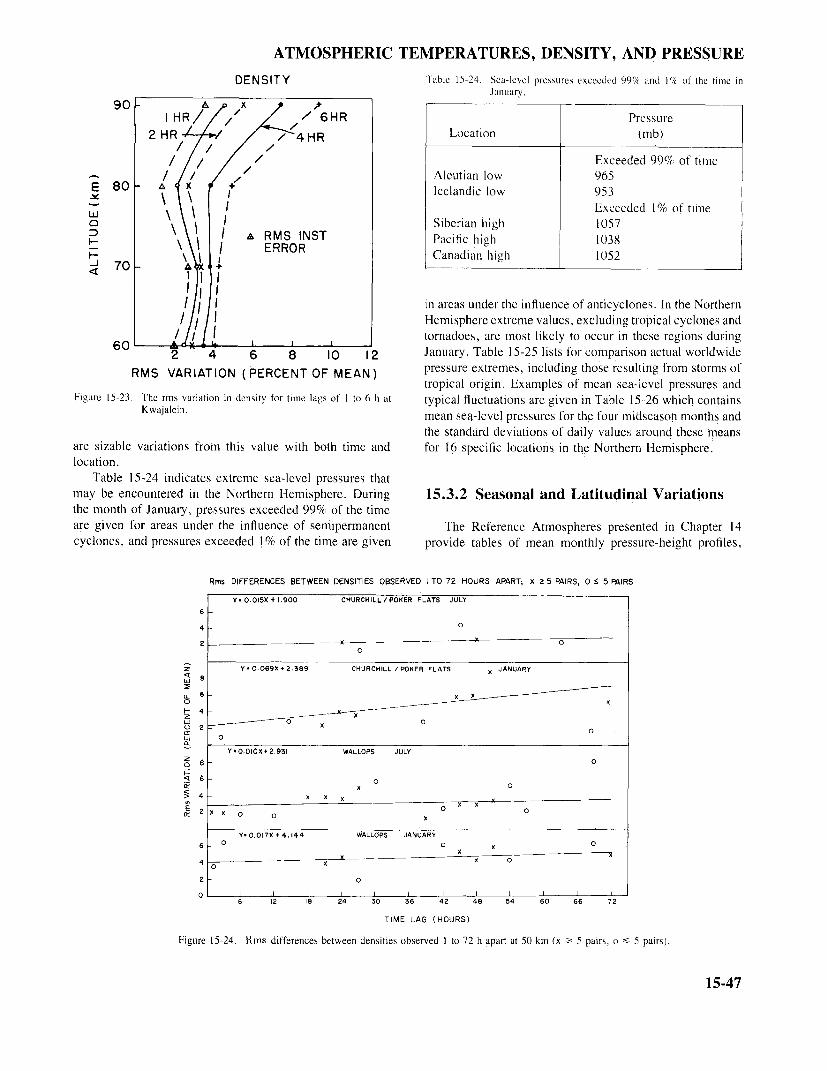
ATMOSPHERIC TEMPERATURES, DENSITY, AND PRESSURE

DENSITY Table 15-24. Sea-level pressures exceeded 99% and 1% of the time inJanuary

90 HAR9 I /HR /// //6HR .Pressure

2 HR /4HR Location (mb)2HR~ "//~/HR/// / // / / / Exceeded 99% of time

80 ~~~~~~~/ / / +Aleutian low 96580 +/E 8 \ \ I Icelandic low 953_'"~ \ \ I lExceeded 1% of timeJIJ

Q I Siberian high 1057v\ [ A ~RMS INST Pacific high 1038

I I ERROR\\I I E0RRO _NSTCanadian high 1052I- ~~~~~~~~~~~~~~~~~~~~1052-J 70 A , +

'II II 11 I in areas under the influence of anticyclones. In the Northern

fI lHemisphere extreme values, excluding tropical cyclones and

60 _I $ l ' ' 'tornadoes, are most likely to occur in these regions during2 4 6 8 10 12 January. Table 15-25 lists for comparison actual worldwide

RMS VARIATION (PERCENT OF MEAN) pressure extremes, including those resulting from storms oftropical origin. Examples of mean sea-level pressures and

Figure 15-23. The rms variation in density for time lags of I to 6 h at typical fluctuations are given in Table 15-26 which containsKwajalein . ~~~~~Kwajalei ~n. ~mean sea-level pressures for the four midseason months and

the standard deviations of daily values around these meansare sizable variations from this value with both time and for 16 specific locations in the Northern Hemisphere.location.

Table 15-24 indicates extreme sea-level pressures thatmay be encountered in the Northern Hemisphere. During 15.3.2 Seasonal and Latitudinal Variationsthe month of January, pressures exceeded 99% of the timeare given for areas under the influence of semipermanent The Reference Atmospheres presented in Chapter 14cyclones, and pressures exceeded 1% of the time are given provide tables of mean monthly pressure-height profiles,

Rms DIFFERENCES BETWEEN DENSITIES OBSERVED I TO 72 HOURS APART; X > 5 PAIRS, 0 < 5 PAIRS

Y. 0.015X + 1.900 CHURCHILL/POKER FLATS JULY

6

4 0

02 ~~~ ~ ~~~~~~~x x So

Y- 0.069X+ 2.389 CHURCHILL / POKER FLATS X JANUARYL.J

/4 6 x X

I- 420

Y · O.O0OX + 2.931 WALLOPS JULYZa o

0 o4 X X X

2 X Xo 0 0

Y- 0.017X + 4.14 4 WALLOPS JANUARY6 0 0 X Oa:4 X 0200

0 IJ I JJ IIII I I I I6 12 1a 24 30 36 42 48 5

4 60 66 72

TIME LAG (HOURS)

Figure 15-24. Rms differences between densities observed I to 72 h apart at 50 km (x 5 pairs, o 5 pairs).

15-47

CHAPTER 15

Table 15-25. Worldwide pressure extremes.

Pressure(mb) Location Date

LOWWorld 870* 17°N, 138°E, Typhoon Tip [Wagner, 1980] 12 Oct 1979

876* 13°N, 141°E, Typhoon June [Holliday, 1976] 19 Nov 1975877* 190N, 135°E. Typhoon Ida [Riordan, 1974] 24 Sep 1958877* 15°N, 128°E, Typhoon Nora [Holliday, 1975] 6 Oct 1973

No. America 892.3 Matecumbe Key, Florida, hurricane [Riordan, 1974] 2 Sep 1935

HIGHWorld 1083.8 Agata, Siberia [Riordan, 1974] 31 Dec 1968

1075.2 Irkutsk, Siberia, [Valley, 1965] 14 Jan 1893No. America 1067.3 Medicine Hat, Alberta [Riordan, 1974] 24 Jan 1897

*Dropsonde measurements

surface to 90 km, for 15° intervals of latitude from the ences are small and do not display a systematic seasonalequator to the north pole. These atmospheric models de- pattern. Departures from standard generally increase withscribe both seasonal and latitudinal variation of pressure. latitude. Thus, largest seasonal differences are shown atFigure 15-25 contain the vertical pressure profiles for the 60°N where mean monthly pressures at 60 to 70 km aremidseason months at each of four latitudes: 15°, 30° , 45° nearly 40% greater than standard in July and 30% to 36%and 60°N. The profiles are displayed as percent depar- less than standard in January. Consequently, July valuestures from the U.S. Standard Atmosphere, 1976. Pres- are roughly twice those in January between 60 and 70sures at altitudes between 2 km and 70 or 80 km are km. Pressures at these levels at 75°N (not shown) arehighest in summer and lowest in winter over regions roughly 10% lower than these values in winter and 15%poleward of 30°N. In tropical latitudes, seasonal differ- higher in summer.

Table 15-26. Mean monthly sea-level pressures and standard deviations of daily values.

Location January April July October

Mean S.D. Mean S.D. Mean S.D. Mean S.D.Latitude Longitude (mb) (mb) (mb) (mb) (mb) (mb) (mb) (mb)

10°N 70°W 1013 2 i012 1 1012 1 1011 120°N 70°W 1018 2 1017 2 1018 2 1013 230°N 70°W 1022 6 1019 5 1021 3 1018 440°N 70°W 1018 10 1017 9 1016 5 1018 850°N 70°W 1016 12 1014 10 1011 6 1013 1160°N 70°W 1008 11 1014 10 1008 7 1008 10700N 70°W 1004 11 1014 10 1009 6 1006 1080°N 70°W 1011 11 1020 9 1011 6 1013 8

100N 20°E 1012 4 1008 3 1009 2 1009 220°N 200 E 1017 4 1011 3 1008 2 1012 230°N 200E 1019 5 1014 4 1012 3 1015 340°N 200E 1018 9 1013 6 1013 3 1016 550°N 20°E 1020 12 1013 7 1013 5 1017 860°N 200E 1015 16 1012 10 1011 7 1011 1170°N 200E 1004 15 1010 10 1012 7 1005 1180°N 200E 1008 15 1016 10 1014 7 1010 10

15-48

ATMOSPHERIC TEMPERATURES, DENSITY, AND PRESSURE

60°N 45°N 30

°N 15

0N

so - // I ' JAN

~~~ // ~~~~~~~ // /1 ~~~~~~~~~JUL/ " 7// /:70 /-I

OCT.7ol

E JAN OFT APR JUL JAN OCT APR JUL JAN APR JUL

50 - I

/I..I~~~~~~~~~~~~~~~~, I.I~~~ ' :

30 I-

20 2J I I

PERCENT DEPARTURE FROM US STANDARD ATMOSPHERE

Figure 15-25. Pressure-altitude profiles for midseason months.

Table 15-27. Average height and standard deviation at standard pressure levels over North America. 90 to 1000 W.

Average Height and Standard Deviation

20'N 30'N 40'N 50'N 60'N 70'N 80'NPressure Mean S. D. Mean S. D. Mean S. D. Mean S.D. Mean S.D. Mean S. D. M'ean S. D.

(mb) (kin) (in) (kin) (in) (kin) (in) (kin) (in) (kin) (in) (kin) (in) (k m) (in)

January

700 3.165 30 3.115 55 3.015 85 2.865 100 2.770 100 2.710 90 2.690 75500 5.845 40 5.745 85 5.565 125 5.340 145 5.1 80 150 5.075 140 5.055 125300 9.595 55 9.425 125 9.150 175 8.825 195 8.585 230 8.425 210 8.380 180200 12.280 70 12.090 130 11.765 165 11.430 175 11.180 190 10.995 200 10.920 195100 16.455 55 16.325 95 16, 110 110 15.890 145 15.655 175 15.400 195 15. 195 19050 20.540 130 20.500 200 20.415 215 20.280 215 20.075 200 19.775 180 19.440 18025 24.900 210 24.865 245 24.790 335 24.555 275 24.380 245 23.905 245 23.425 23015 28.100 245 28.050 335 28.000 365 27.750 365 27.650 350 27.000 335 26.350 30510 30.600 250 30.550 380 30.500 400 30.250 380 30.150 380 29.500 320 28.750 260

July

700 3.185 IS 3.190 20 3.170 35 3.080 55 3.005 60 2.975 65 2.930 65

500 5.890 20 5.910 25 5.875 50 5.720 85 5.600 90 5.540 90 5.465 95300 9.675 30 9.705 35 9.630 80 9,405 130 9.215 125 9.125 125 9.010 130200 12.395 40 12.430 50 12.345 100 12.080 135 11.870 135 11.790 135 11.710 135100 16.570 45 16.625 50 16.605 65 16.515 80 16.455 85 16.420 80 16.390 7550 20.765 75 20.865 90 20.940 105 20.975 lOS 21.005 105 21.045 90 21.050 7525 25. 180 ISO 25.330 150 25.440 175 25.530 175 25.625 165 25.715 ISO 25.765 ISOIS 28.300 170 28.450 170 28.650 175 28.800 175 28.900 175 29.10(0 170 29.200 16510 30.800 190 30.950 190 31.200 190 31.400 190 31.550 190 3 1.75(0 185 31.950 ISO

15-49

CHAPTER 15

Table 15-28. Departures from mean monthly pressures (%) exceeded less than 5% of the time in January and July. Values below 30 km are based onradiosonde observations. Those values above 30 km are based on rocketsonde observations

Height January July

(km) 75°N 60°N 45°N 30°N 15°N 15°N 30°N 45°N 60°N 75°N

0 +2.5 +3 _2.5 + I +0.4 +0.4 +0.5 + 1 + + 1.510 7 4 3 2 0.8 0.7 0.8 2 3 420 10 10 10 7 4 2 2 3 3 330 20 16 14 12 7 4 4 4 5 5

40 25 20 15 8 7 8 8 1050 30 25 18 10 10 12 13 1460 35 30 20 12 12 14 16 1870 30 25 18 10 10 12 15 1680 20 16 12 8 8 9 10 10

Table 15-29. Amplitudes of systematic pressure variations and time ofmaximum at Terceira, Azores [Harris et al, 1962].

15.3.3 Day-to-Day Variations Diurnal SemidiurnalDiurnal Semidiurnal

Changing synoptic situations, which include movements Pressure Level Ampi. Time Ampl. Timeof high and low pressure centers and their associated ridges (mb) (m)* (mb) (h) (mb) (h)and troughs, and variations in the energy absorbed directlyby the atmosphere, cause day-to-day changes in the height $f 1 0 0.10 2100 0.50 0948Sfc0 12 0.10 21904 0.50 0950of constant pressure surfaces. Information on the magnitude 0 0.1 14 0. 0951000 570 0.12 1824 0.46 0956of day-to-day variations in the heights of such surfaces are 900 5703 0.16 16124 0.49 10956provided in this section. Detailed information for specific 900 1033 0.16 1612 0.49 1002

850 1454 0.18 1604 0.47 1002levels and locations should be requested if conditions appear 80 0. 16 0.4 1002critical. critical . ~~~~~~~~~800 2027 0.20 1612 0.44 1002750 2569 0.20 1616 0.38 1010Table 15-27 lists monthly mean heights of pressure sur- 750 2569 0.20 1616 0.38 1010faces in January and July and their standard deviations for 700 3127 0.25 1548 0.37 1002650 3712 0.25 1608 0.407 100middle North America. These data indicate the variation in 650 3731 0.18 1608 0.40 1030600 43731 0.25 1608 0.33 1020the mean heights of constant pressure surfaces between 700 600 4365 0.25 1608 0.33 1020

550 5051 0.27 1508 0.33 1034and 10 mb with latitude and season, and the estimated dis- 50 5 0.2 15 0. 103500 5782 0.28 156 0.29 1032tributions of day-to-day variability around the monthly means.

Estimated departures from mean monthly pressures, which 450 6587 0.27 1424 0.24 1036400 7449 0.31 1504 0.24 1046are equaled or exceeded less than 5% of the time between 0 49 0.31 1504 0.2 1046

15° and 75°N, are shown in Table 15-28 as percentages of 350 8409 0.31 1504 0.20 1046300 9482 0.32 1444 0.18 1108the mean January and July values, surface to 80 km. 300 9482 0.32 1444 0.18 8250 10708 0.33 1420 0.16 1102As can be seen in Table 15-28, day-to-day variability 20 1 0.3 140 0.1 110200 12149 0.32 1408 0.14 1110generally increases with latitude and altitude in both January 121 0.32 1 0.1 110175 12991 0.32 1352 0.13 1120and July, although to a much smaller extent in July. The 15 19 0.3 13 0.1 110

estimated 5% extremes are largest at 60 to 65 km at all 150 13948 0.30 1348 0.11 1100latitudes, reaching +35% during 60°N winter. Variability 125 15066 0.28 1328 0.11 1124125 15646 0.26 1304 0.09 1128appears to decrease above 65 km to a probable minimum 16423 0.26 1304 0.09 1128100 17776 0.24 1300 0.09 1120value near 85 km. The estimated departures shown in Table 80 7776 0.24 1300 0.09 112060 19547 0.23 1256 0.07 112415-28 include some diurnal and semidiurnal fluctuations due 60 19547 0.23 1256 0.07 1124

50 20668 0.21 1256 0.07 1114to solar influences, particularly since the basic pressure data 50 20668 0.21 1256 0.07 111440 22077 0.20 1244 0.06 1116were not observed at the same time every day. Envelopes 40 22077 0.20 1244 0.06 1116

of these estimated 95% values should not be used as profiles 30 24012 0.18 1256 0.05 111020 26673 0.16 1256 0.04 1128since such pressures would not necessarily be found at all 20 26673 0.16 1256 0.04 1128

altitudes at any one given time and/or location. Decreases 15 28005 0.15 1252 0.03 1136in atmospheric pressure in one layer, for example, normally 10 30507 0.12 1304 0.01 1204are associated with increases in another layer. *Estimated mean annual height

15-50

ATMOSPHERIC TEMPERATURES, DENSITY, AND PRESSURE

15.3.4 Diurnal and Semidiurnal Variations Upper-air pressures appear to follow a systematic diur-nal/semidiurnal cycle similar to that at sea level; however,extremes occur at somewhat different hours. Table 15-29

Mean hourly sea-level pressures follow a systematic lists amplitudes and times of occurrence of diurnal and sem-diurnal and semidiurnal periodicity somewhat variable in idiurnal maxima to 10 mb (roughly 30 km) over Terceira,amplitude and phase according to location and season. The Azores, which provides an estimate of mean annual sys-sea-level pressure cycle is generally characterized by min- tematic pressure variations at a maritime location near 40°N.ima near 0400 and 1600 hours and maxima near 1000 and The semidiurnal variations at climatically and geographi-2200 hours local time. The amplitude approaches 1 mb, cally different locations such as Washington, D.C. and Ter-which is small relative to synoptic changes in middle lati- ceira, Azores, appear to be similar [Valley, 1965]. Thetudes. In the tropics only minor synoptic changes occur from diurnal maxima and minima, however, that result from solarday to day, so that interdiurnal pressure changes are small insolation and terrestrial radiation, may differ considerablycompared to the systematic daily variations in these lati- in time of occurrence and amplitude at various locations,tudes. particularly at or near surface levels.

15-51

CHAPTER 15

REFERENCES - CHAPTER 15

Albrecht, F., "Micrometeorologische Temperaturmessun- denen Boeden unter Gleichen Witerungs Verhaeltnis-gen von Flugzeug aus," Ber. Deutsch Wetterd, Bad Kis- ser," Zeitschr, f. angewandte Meteorologie, 60: 65, 1943.singen, 38: 332, 1952. Lettau, H., "A Study of the Mass, Momentum and Energy

Bertoni, E.A. and I.A. Lund, "Winter Space Correlations Budget of the Atmosphere," Archiv fur Meteorologie,of Pressure, Temperature and Density of 16 km," AFCRL- Geophysik and Bioklimatologie, Serie A, 7:133, 1954a.64-1020, ADA611002, 1964. Lettau, H., "Improved Models of Thermal Diffusion in the

Cole, A.E. "Review of Data and Models of the Middle Soil," Trans. AGU, 35: 121, 1954b.Atmosphere," Space Research, 20 1979. National Weather Service, "Surface Observations," Federal

Cole, A.E. and A.J. Kantor, "Tropical Atmospheres, 0 to Meteorological Handbook 90-1, Government Printing90 km," AFCRL TR-75-0527, ADA019940, 1975. Office, Washington, D.C., 1979.

Cole, A.E. and A.J. Kantor, "Interlevel Correlations of Riordan, P., Weather Extremes Around the World, ReportTemperature and Density, Surface to 60 km," AFGL ETL-TR-74-5, U.S. Army Engineering TopographicTR-80-0163, ADA090515, 1980. Laboratories, Ft. Belvoir, Va., 1974.

Cole, A.E., A.J. Kantor, and C.R. Philbrick, "Kwajalein Singer, I.A. and R.M. Brown, "Annual Variation of Sub-Reference Atmospheres, 1979," AFGL TR-79-0241, Soil Temperatures About a 600-Foot Diameter Circle,"ADA081780 1979. Trans. AGU, 37: 743, 1956.

Davidson, B. and H. Lettau (eds.), Great Plains Turbulence Sissenwine N. and A. Court, "Climatic Extremes for Mil-Field Program, Pergamon Press, New York, 1957. itary Equipment," Env. Protection Br., Rpt. No. 146,

Draeger, R.H. and R.H. Lee, "Meteorological Data Eni- Dept. of Army, Washington, D.C., 1951.wetock Atoll," Naval Medical Res. Inst. Memo Rept. Tattelman, P., "Duration of Cold Temperature Over North53-8, Bethesda, Md, 1953. America," AFCRL-68-0232, AD669567, 1968.

Geiger, R., The Climate Near the Ground, Harvard Uni- Tattelman, P. and A.J. Kantor, "Atlas of Probabilities ofversity Press, Translated by M.N. Stewart et al., 1957. Surface Temperature Extremes: Part I, Northern Hemi-

Gringorten, I.I., "Probability Models of Weather Conditions sphere," AFGL TR-76-0084, ADA027640, 1976aOccupying a Line or an Area," J. Appl. Meteorol., 18: Tattelman, P. and A.J. Kantor, "Atlas of Probabilities of957, 1979. Surface Temperature Extremes: Part II, Northern Hemi-

Harris, M.F., F.G. Finger, and S. Teweles, "Diurnal Vari- sphere," AFGL TR-77-0001, ADA038237, 1976b.ation of Wind, Pressure and Temperature in the Trop- Tattelman, P. and A.J. Kantor, "A Method for Determiningosphere and Stratosphere over the Azores," J. Atmos Probabilities of Surface Temperature Extremes," J. Appl.Sci., 19: 136, 1962. Meteorol., 16: 175, 1977.

Holliday, C.R., "An Extreme Sea-level Pressure Reported Tattelman, P., N. Sissenwine, and R.W. Lenhard, Jr., "Worldin a Tropical Cyclone," Monthly Weather Rev., 103: Frequency of High Temperature," AFCRL-69-0348,163, 1975. AD696094, 1969.

Holliday, C.R., "Typhoon June -Most Intense on Re- Valley, S. (ed.), Handbook of Geophysics and Space En-cord," Monthly Weather Rev., 104: 1188, 1976. vironments, AFCRL, 1965.

Kantor, A.J. and A.E. Cole, "Time and Space Variations Wagner, A.J., "Weather and Circulation of October 1979,"of Density in the Tropics," AFGL TR-79-0109, Monthly Weather Rev., 108: 119, 1980.ADA074472, 1979. WMO, "Proceedings of the World Climate Conference, Ge-

Kreutz, W., "Der Jahresgang der Temperatur in Verschie- neva, 12-23 Feb 1979," WMO Report No. 537, 1979.

15-52