remote sensing

Article

Atmospheric Corrections and Multi-ConditionalAlgorithm for Multi-Sensor Remote Sensing ofSuspended Particulate Matter in Low-to-HighTurbidity Levels Coastal Waters

Stéfani Novoa 1, David Doxaran 1,*, Anouck Ody 1, Quinten Vanhellemont 2, Virginie Lafon 3,Bertrand Lubac 4 and Pierre Gernez 5

1 Laboratoire d’Océanographie de Villefranche, UMR7093 CNRS/UPMC, 181 Chemin du Lazaret,06230 Villefranche-sur-Mer, France; snovoa@gmail.com (S.N.); Anouck.Ody@obs-vlfr.fr (A.O.)

2 Royal Belgian Institute of Natural Sciences, Brussels 1000, Belgium;quinten.vanhellemont@naturalsciences.be

3 GEO-Transfert, UMR 5805 Environnements et Paléo-environnements Océaniques et Continentaux (EPOC),Université de Bordeaux, Allée Geoffroy Saint-Hilaire, 33615 Pessac, France; virginie.lafon@i-sea.fr

4 UMR CNRS 5805 EPOC, OASU, Université de Bordeaux, site de Talence, Bâtiment B18,Allée Geoffroy Saint-Hilaire, 33615 Bordeaux Cedex, France; b.lubac@epoc.u-bordeaux1.fr

5 Mer Molécules Santé (EA 2160 MMS), Université de Nantes, 2 rue de la Houssinière BP 92208,44322 Nantes Cedex 3, France; Pierre.Gernez@univ-nantes.fr

* Correspondence: doxaran@obs-vlfr.fr; Tel.: +33-4-9376-3724

Academic Editors: Yunlin Zhang, Claudia Giardino, Linhai Li, Xiaofeng Li and Prasad S. ThenkabailReceived: 20 September 2016; Accepted: 3 January 2017; Published: 12 January 2017

Abstract: The accurate measurement of suspended particulate matter (SPM) concentrations in coastalwaters is of crucial importance for ecosystem studies, sediment transport monitoring, and assessment ofanthropogenic impacts in the coastal ocean. Ocean color remote sensing is an efficient tool to monitorSPM spatio-temporal variability in coastal waters. However, near-shore satellite images are complexto correct for atmospheric effects due to the proximity of land and to the high level of reflectancecaused by high SPM concentrations in the visible and near-infrared spectral regions. The waterreflectance signal (ρw) tends to saturate at short visible wavelengths when the SPM concentrationincreases. Using a comprehensive dataset of high-resolution satellite imagery and in situ SPM andwater reflectance data, this study presents (i) an assessment of existing atmospheric correction (AC)algorithms developed for turbid coastal waters; and (ii) a switching method that automatically selectsthe most sensitive SPM vs. ρw relationship, to avoid saturation effects when computing the SPMconcentration. The approach is applied to satellite data acquired by three medium-high spatialresolution sensors (Landsat-8/Operational Land Imager, National Polar-Orbiting Partnership/VisibleInfrared Imaging Radiometer Suite and Aqua/Moderate Resolution Imaging Spectrometer) to mapthe SPM concentration in some of the most turbid areas of the European coastal ocean, namely theGironde and Loire estuaries as well as Bourgneuf Bay on the French Atlantic coast. For all threesensors, AC methods based on the use of short-wave infrared (SWIR) spectral bands were tested,and the consistency of the retrieved water reflectance was examined along transects from low- tohigh-turbidity waters. For OLI data, we also compared a SWIR-based AC (ACOLITE) with a methodbased on multi-temporal analyses of atmospheric constituents (MACCS). For the selected scenes,the ACOLITE-MACCS difference was lower than 7%. Despite some inaccuracies in ρw retrieval, wedemonstrate that the SPM concentration can be reliably estimated using OLI, MODIS and VIIRS,regardless of their differences in spatial and spectral resolutions. Match-ups between the OLI-derivedSPM concentration and autonomous field measurements from the Loire and Gironde estuaries’monitoring networks provided satisfactory results. The multi-sensor approach together with themulti-conditional algorithm presented here can be applied to the latest generation of ocean color

Remote Sens. 2017, 9, 61; doi:10.3390/rs9010061 www.mdpi.com/journal/remotesensing

Remote Sens. 2017, 9, 61 2 of 31

sensors (namely Sentinel2/MSI and Sentinel3/OLCI) to study SPM dynamics in the coastal ocean athigher spatial and temporal resolutions.

Keywords: remote sensing; suspended particulate matter; coastal waters; river plumes;multi-conditional algorithm

1. Introduction

The quality of coastal and estuarine waters is increasingly under threat by the intensification ofanthropogenic activities. For that reason, the European Union Marine Strategy Framework Directive(MSFD, 2008/56/EC) and Water Framework Directive (WFD, 2000/60/EC and amendments) requiremember states to monitor the quality of the marine environment and to achieve and maintain a goodenvironmental status of all marine waters by 2020. The directives require member states to assessthe ecological quality status of water bodies, based on the status of several elements, including watertransparency. Rivers serve as the main channel for the delivery of significant amounts of dissolvedand particulate materials from terrestrial environments to the ocean. Along with freshwater, theydischarge suspended particulate matter (SPM) that modifies the color and transparency of the water.In addition, SPM is associated with metallic contaminants and bacteria that affect water quality. Hence,monitoring the spatio-temporal distribution of SPM in estuarine and coastal waters is of particularimportance, not only to assess water transparency, but also to evaluate the impacts of human activities(e.g., transport of pollutants, dams, offshore wind farms, sand extraction, watershed management)and to study sediment transport dynamics.

SPM field measurements are time-consuming, expensive and specific to a time and/or geographicallocation, and therefore do not always accurately represent the temporal and spatial dynamics of river,estuarine or coastal systems. Ocean color remote sensing onboard satellite platforms can be very usefulto complement field measurements and monitor surface SPM transport in natural waters [1–14]. Mostsatellite-borne sensors provide a spectral resolution covering the visible and near-infrared (NIR)spectral regions required for atmospheric corrections of satellite data, and for the estimation ofbiogeochemical material such as SPM (e.g., [15,16]). Sensors such as SPOT (Satellite Pour l’Observationde la Terre) and Landsat-8/OLI (Operational Land Imager), designed for land applications, providehigh-spatial-resolution imagery, and their potential for mapping the concentration of SPM inhighly turbid waters has been demonstrated [17–19]. These high-resolution sensors combined withhigh-temporal-resolution satellite data [20,21] have proved to provide valuable information regardingSPM dynamics.

An important issue regarding satellite remote sensing in coastal and estuarine areas is atmosphericcorrection (AC) failures when applying standard algorithms designed for open ocean methods. This iscaused by the presence of high water turbidity and also by the proximity to land. To achieve anaccurate atmospheric correction, the top-of-the-atmosphere signal recorded by satellite sensors isseparated into marine, gaseous and aerosol contributions. Typical open ocean atmospheric correctionmethods assume the marine signal to be zero in the near-infrared (NIR) bands due to very high lightabsorption by pure water and very low light backscattering by suspended particles [22]. The signal inthe NIR bands is used to determine an aerosol model, which is then used to extrapolate the aerosolreflectance to visible bands. In turbid waters, the contribution of light backscattering by particles isno longer negligible in the NIR region compared to light absorption. This results in a non-negligiblewater reflectance signal, an overestimation of the aerosol reflectance, and underestimated or negativewater reflectance values in visible bands [23]. Studies have focused on two approaches to developatmospheric corrections over turbid waters: one is to model the marine contribution in the NIRbands [23,24] and the other involves the use of short-wave infrared (SWIR) bands, where the watersignal can be assumed to be zero even in turbid coastal waters [25].

Remote Sens. 2017, 9, 61 3 of 31

For low to moderately turbid waters, a good correlation is found between the SPM concentrationand water reflectance (ρw) in the green and red parts of the spectrum (refer to [16]). The correspondingwavebands of wide-swath ocean color instruments, such as the Orbview-2/Sea-viewing Wide Field-of-viewSensor (SeaWiFS), the Aqua/Moderate Resolution Spectrometer (MODIS), the ENVISAT/MediumSpectral Resolution imaging spectrometer (MERIS), the Landsat/Enhanced Thematic Mapper Plus(ETM+) and OLI, and the Visible Infrared Imaging Radiometer Suite (VIIRS), have therefore beensuccessfully used to map SPM in coastal waters for concentrations below ~60 g·m−3 [6,13,26–28].In highly turbid waters (SPM higher than ~60 g·m−3), a saturation of the water reflectance in the greenand red bands is usually observed, so a NIR band should be considered to establish relationshipswith SPM [4,18,29,30]. There are three main types of algorithms commonly used to derive SPMconcentration from water reflectance: (1) empirical, (2) semi-analytical and (3) analytical algorithms.Empirical single-band and band-ratio models have been commonly used in coastal and estuarineareas [6,31]. These types of models are dependent on SPM and reflectance ranges, and requirecalibration with regional measurements. Semi-analytical or analytical models are based on the inherentoptical properties (IOPs) and provide a more global application [16,32,33]. However, they can belimited by the validity and accuracy of the hypotheses chosen to model the IOPs. Hence, providedthe large choice of SPM algorithms, it is difficult to select one model that will provide accurate SPMconcentration retrieval from low- to high-turbidity waters, limiting the study of SPM dynamics overlarge coastal areas. For that reason, some studies have focused on multi-conditional algorithm schemescomposed of several SPM models, as they have been shown to provide a more effective and accurateestimation of SPM over a wide range of turbid waters [34–37]. The difficulty resides in the selectionof the proxies and the limiting bounds for each model. Some studies have used ranges of SPMconcentration as switching thresholds [35] and others have used reflectance values [36], but the boundsare generally selected through trial and error.

The main objective of this study is to determine the boundaries for switching between differentSPM models, based on band comparisons from field water reflectance measurements, then apply thisswitching algorithm to ocean color satellite data to derive SPM across low- to high-turbidity waters.Since atmospheric correction is a major issue in coastal areas, different atmospheric correction methodsare tested for several study areas and sensors, and the most appropriate one is selected. To achievethese aims, this study will focus on three objectives.

(1) To compare atmospheric correction algorithms for OLI, VIIRS and MODIS satellite data over twostudy areas covering low- to high-turbidity waters;

(2) To develop a reliable multi-conditional algorithm to retrieve SPM from satellite imagery over awide range of turbidity values and apply it to satellite data;

(3) To inter-compare multi-sensor satellite products (ρw and SPM) over turbid coastal, estuarine andriver waters.

Two case studies are considered: the Loire Estuary, with the adjacent Bourgneuf Bay, and theGironde Estuary. For both areas, high quality ρw and SPM measurements are available. The paper isorganized as follows: first, the methodology for the application of different SPM models over the studyareas is developed. Second, a comparison between different atmospheric corrections is presented.Finally, the developed multi-conditional algorithm is applied to atmospherically corrected imageryfrom multiple satellite sensors.

2. Materials and Methods

2.1. Study Areas

This study covers two areas with a wide range of SPM concentration from low to highly turbidwaters (Figure 1). The Gironde Estuary, located in South Western France, is one of the largest estuariesin Europe (length of 90 km and width 3–11 km). It is formed by the confluence of the Garonne

Remote Sens. 2017, 9, 61 4 of 31

and Dordogne rivers. These rivers’ watersheds represent 57,000 km2 and 24,000 km2, and theysupply respectively 65% and 35% freshwater inputs into the Estuary. The Garonne’s freshwaterdischarge ranges from less than 100 m3·s−1 to more than 4000 m3·s−1, while the Dordogne dischargefluctuates between 200 and 1500 m3·s−1 [38]. The Gironde’s flow rate averages 1100 m3·s−1 andits morphology is typical of a macro-tidal estuary (tidal ranges from 2 to 5 m) impacted by waves.It presents a well-developed turbidity maximum zone formed from tidal asymmetry and densityresidual circulation [39]. The SPM concentration within surface waters range from about 1 to 50 g·m−3

in the plume [40] and from 50 to approximately 3000 g·m−3 in the estuary [41,42].The Loire is the largest river in France: it is 1012 km long and has a watershed area of 117,000 km2.

Its flow rate ranges between 300 m3·s−l during the summer droughts and 4000 m3·s−l during winterfloods. The Loire Estuary is 100 km long and has a macro-tidal regime, with a 4 m mean tidal amplitude.It is characterized by high SPM concentration variations, ranging from 50 to more than 1000 g·m−3

within surface waters. South from the Loire Estuary, Bourgneuf Bay is a macro-tidal bay with a tidalrange between 2 and 6 m. The bay has an area of 340 km2, of which 100 km2 are intertidal area mostlyoccupied by mudflats. Due to tidal re-suspension, mudflat and adjacent waters are highly turbid.Bourgneuf Bay is an important oyster-farming site, but in some sectors high SPM concentration mayhave a negative impact on oyster aquaculture [43].

Remote Sens. 2017, 9, x FOR PEER REVIEW 4 of 33

morphology is typical of a macro-tidal estuary (tidal ranges from 2 to 5 m) impacted by waves. It presents a well-developed turbidity maximum zone formed from tidal asymmetry and density residual circulation [39]. The SPM concentration within surface waters range from about 1 to 50 g·m−3 in the plume [40] and from 50 to approximately 3000 g·m−3 in the estuary [41,42].

The Loire is the largest river in France: it is 1012 km long and has a watershed area of 117,000 km2. Its flow rate ranges between 300 m3·s−l during the summer droughts and 4000 m3·s−l during winter floods. The Loire Estuary is 100 km long and has a macro-tidal regime, with a 4 m mean tidal amplitude. It is characterized by high SPM concentration variations, ranging from 50 to more than 1000 g·m−3 within surface waters. South from the Loire Estuary, Bourgneuf Bay is a macro-tidal bay with a tidal range between 2 and 6 m. The bay has an area of 340 km2, of which 100 km2 are intertidal area mostly occupied by mudflats. Due to tidal re-suspension, mudflat and adjacent waters are highly turbid. Bourgneuf Bay is an important oyster-farming site, but in some sectors high SPM concentration may have a negative impact on oyster aquaculture [43].

Figure 1. Maps of the study areas: Bourgneuf Bay and Loire Estuary (a) and Gironde Estuary and plume area (b). Red squares show the location of the in situ measurements performed during the optical cruises. Black squares show the location of the monitoring stations used for match-ups between satellite and in situ data.

(a) (b)

Figure 1. Maps of the study areas: Bourgneuf Bay and Loire Estuary (a) and Gironde Estuary andplume area (b). Red squares show the location of the in situ measurements performed during theoptical cruises. Black squares show the location of the monitoring stations used for match-ups betweensatellite and in situ data.

2.2. Multi-Conditional SPM Algorithm Development

2.2.1. In Situ SPM and Reflectance Data

Field measurements used for the calibration of SPM models and multi-conditional algorithmwere carried out during four bio-optical cruises (from April 2012 to July 2014) in the two selected test

Remote Sens. 2017, 9, 61 5 of 31

sites: the SeaSWIR (2012, 2013) and Rivercolor (2014) surveys in the Gironde Estuary area and theGigassat (2013) survey in Bourgneuf Bay. Additionally, several measurements conducted in April 2016in the Bourgneuf-Loire area were used to increase the number of match-ups between satellite and insitu data.

At each station, hyperspectral reflectance measurements were carried out using TriOS-RAMSESradiometers in the same way as the methodology described in [13]. The protocol described in [44]based on the NASA (National Aeronautics and Space Administration) protocols [45] to computethe remote sensing reflectance (Rrs, sr−1). Rrs spectra of five successive measurements under stableillumination (i.e., downwelling irradiance variations between two measurements lower than 15%) anddiffering less than 25% from the median of all the spectra, were selected and averaged. A total of 67 Rrs

spectra were finally selected for the Gironde Estuary and 29 for Bourgneuf Bay.Simultaneously with the reflectance measurements, water samples were collected with a bucket at

about 0.5 m depth. They were directly filtered with pre-weighed Whatman GF/F filters to determinethe SPM concentration with the gravimetric method procedure described in [46], based on [47]. ThreeSPM measurement replicates were conducted per station, and the standard deviation obtained fromthose measurements were used as the uncertainty for the SPM concentration (error bars in figures).Water turbidity (measured in nephelometric turbidity units, NTU) was measured for most stationsusing a Hach Portable turbidity meter, following the protocol by [32] SPM and turbidity measurementranges for each location are shown in Table 1. Three replicate measurements of turbidity wereconducted per station to estimate the measurement uncertainties. The SPM vs. turbidity relationshipfor the Gironde Estuary was established using measurements undertaken during the SeaSWIR surveysat the Pauillac station: SPM (g·m−3) = 0.88 × Turbidity (NTU).

Table 1. The distribution of SPM concentration (g·m−3) and turbidity (NTU) values (field measurements)used for the calibration of the models.

SPM (g·m−3) Turbidity (NTU)

Location Mean StandardDeviation Maximum Minimum Mean Standard

Deviation Maximum Minimum

Gironde 347.1 372.7 1579.1 2.6 310.0 24.19 2045.9 1.5Bourgneuf 162.4 90.4 340.6 17.8 100.6 78.47 301.3 12.7

2.2.2. SPM Models

The sets of hyperspectral Rrs in situ measurements acquired in the Gironde area were convolutedto the relative spectral response function of the green, red and NIR OLI bands (5, 4, 3), VIIRS bands(M4, M5, M7), and MODIS bands (B4, B1, B2) as explained in [16] to derive the band-weightedreflectance values. The same procedure was completed for the in situ measurements collectedin Bourgneuf Bay. The resulting Rrs values were then expressed as dimensionless water-leavingreflectance ρw (Rrs × π) values, hereinafter referred as ρ.

Figure 2 shows typical in situ measurements of ρ spectra and corresponding SPM concentration.For concentration between 2.6 and 10.5 g·m−3, the ρ between 400 and 600 nm increases rapidly. Fromthe examples shown in Figure 2, it can be observed that red reflectance is more sensitive than greenreflectance to concentration changes between 10.5 and 119 g·m−3. For SPM above 119 g·m−3, ρ inthe NIR is most sensitive to concentration changes. This implies that models based on the visiblebands are not effective in discriminating SPM in highly turbid waters as demonstrated by previousstudies [18,31].

Remote Sens. 2017, 9, 61 6 of 31

Remote Sens. 2017, 9, 61 6 of 31

(a) (b)

Figure 2. Selected water reflectance spectra (ρ = Rrs × π) for different SPM concentration (g·m−3) measured in the Gironde Estuary (a) and Bourgneuf Bay (b). Vertical bars locate the green, red and NIR bands of the considered satellite sensors

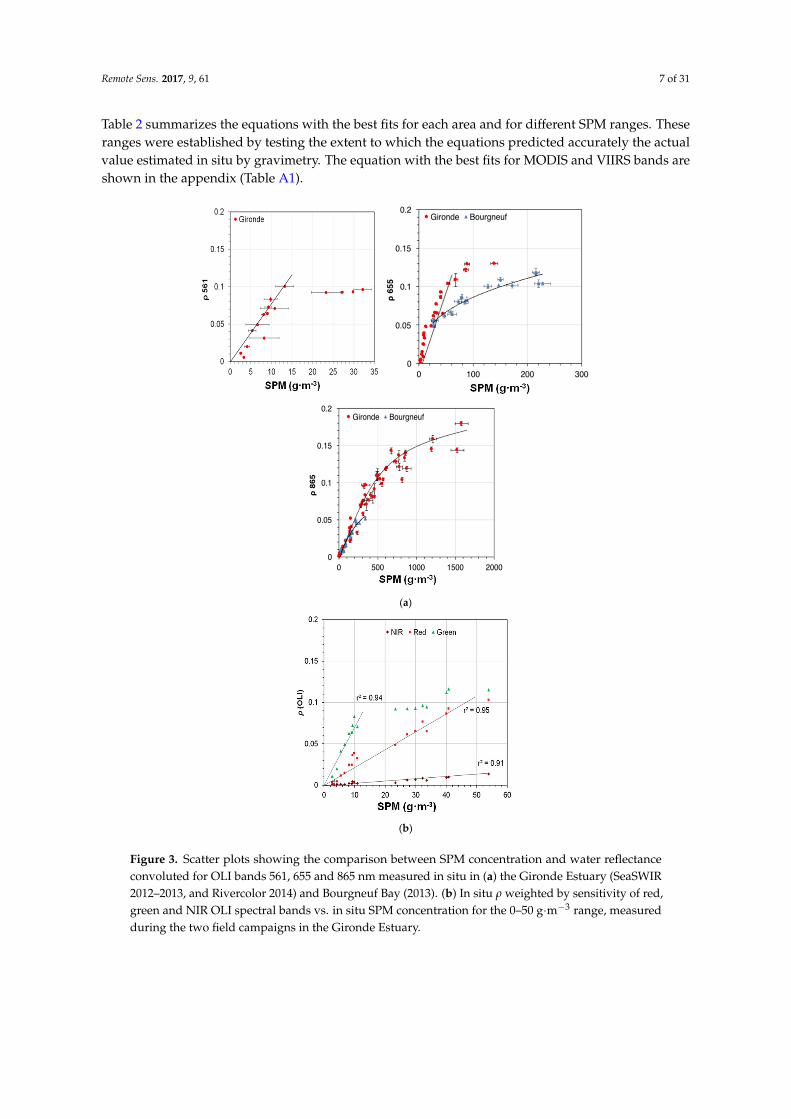
The relationships between ρ (convoluted to OLI bands) and SPM concentration are presented in Figure 3. Analogous relationships were obtained for both MODIS and VIIRS convoluted bands, and are not shown here. Figure 3a shows a linear relationship between ρ in the green band and SPM concentration lower than 10 g·m−3. Above 10 g·m−3, a saturation of ρ is observed in this band. A green band relationship was not established for the Bourgneuf dataset, as low concentration measurements were not available, so the green band relationship obtained for the Gironde was also applied for Bourgneuf Bay.

Water reflectance in the red band is highly sensitive to variations of SPM concentration lower than 50 g·m−3 and presents a good linear correlation (r2 = 0.89). Above 50 g·m−3, a saturation of ρ is observed. The NIR band is less sensitive to SPM concentration below 50 g·m−3, however it presents a very good fit above this limit by means of a polynomial regression (r2 = 0.97 see Table 2). Figure 3b presents the sensitivity differences between the three bands (green, red, NIR) to SPM concentration for the ~0–50 g·m−3 range. There is a sharper increase in reflectance for the green band compared to the red for concentration below ~10 g·m−3, and a sharper increase in red band reflectance compared to the NIR bands for concentration below 50 g·m−3. This figure also shows the saturation of the green band above ~10 g·m−3, so the r2 was computed for the values below that concentration.

Several empirical models using single bands and NIR-red band ratios were considered in this study. The semi-analytical model developed by [16] was also re-calibrated with in situ datasets. Table A2 in the appendix shows all the algorithms tested. The performance of each model was assessed using the coefficient of determination (r2) and the normalized root mean square error (NRMSE, in %) calculated as follows:

% = ∑ , – ,, – , × 100

(1)

where xp and xobs are respectively the model-derived and field-measured SPM concentration, in g·m−3.

In the case of the Gironde Estuary, the dataset (n = 67) was divided into two sets, one for calibration (n = 34) and one validation (n = 33). The NRMSE was computed for the SPM provided by the models with respect to the validation dataset. The best fits and minimum errors were obtained with the empirically-derived polynomial (second order) regression for the NIR band and linear regressions for the red and green bands (Table 2). In the case of Bourgneuf Bay, the best fits were obtained for the NIR band and the semi-analytical equation developed by [16]. Due to the low number of measurements, the Bourgneuf dataset was not separated into calibration and validation sets. Hence, the percent NRMSE (Equation (1)) in this case represents the deviation of the random component within the data. Table 2 summarizes the equations with the best fits for each area and for

0

0.02

0.04

0.06

0.08

0.1

0.12

0.14

0.16

0.18

0.2

350 450 550 650 750 850 950

ρ

Wavelength (nm)

340.64 g.m-3

211.04 g.m-3

171.59 g.m-3

147 g.m-3

28.48 g.m-3

72.17 g.m-3

53.76 g.m-3

Figure 2. Selected water reflectance spectra (ρ = Rrs × π) for different SPM concentration (g·m−3)measured in the Gironde Estuary (a) and Bourgneuf Bay (b). Vertical bars locate the green, red andNIR bands of the considered satellite sensors.

The relationships between ρ (convoluted to OLI bands) and SPM concentration are presentedin Figure 3. Analogous relationships were obtained for both MODIS and VIIRS convoluted bands,and are not shown here. Figure 3a shows a linear relationship between ρ in the green band and SPMconcentration lower than 10 g·m−3. Above 10 g·m−3, a saturation of ρ is observed in this band. A greenband relationship was not established for the Bourgneuf dataset, as low concentration measurementswere not available, so the green band relationship obtained for the Gironde was also applied forBourgneuf Bay.

Water reflectance in the red band is highly sensitive to variations of SPM concentration lowerthan 50 g·m−3 and presents a good linear correlation (r2 = 0.89). Above 50 g·m−3, a saturation of ρ isobserved. The NIR band is less sensitive to SPM concentration below 50 g·m−3, however it presents avery good fit above this limit by means of a polynomial regression (r2 = 0.97 see Table 2). Figure 3bpresents the sensitivity differences between the three bands (green, red, NIR) to SPM concentration forthe ~0–50 g·m−3 range. There is a sharper increase in reflectance for the green band compared to thered for concentration below ~10 g·m−3, and a sharper increase in red band reflectance compared to theNIR bands for concentration below 50 g·m−3. This figure also shows the saturation of the green bandabove ~10 g·m−3, so the r2 was computed for the values below that concentration.

Several empirical models using single bands and NIR-red band ratios were considered in thisstudy. The semi-analytical model developed by [16] was also re-calibrated with in situ datasets.Table A2 in the appendix shows all the algorithms tested. The performance of each model was assessedusing the coefficient of determination (r2) and the normalized root mean square error (NRMSE, in %)calculated as follows:

NRMSE (%) =

√∑N

i=1(Xp,i −Xobs, i)2

N

Xobs, max − Xobs, min× 100 (1)

where xp and xobs are respectively the model-derived and field-measured SPM concentration, in g·m−3.In the case of the Gironde Estuary, the dataset (n = 67) was divided into two sets, one for calibration

(n = 34) and one validation (n = 33). The NRMSE was computed for the SPM provided by the modelswith respect to the validation dataset. The best fits and minimum errors were obtained with theempirically-derived polynomial (second order) regression for the NIR band and linear regressions forthe red and green bands (Table 2). In the case of Bourgneuf Bay, the best fits were obtained for the NIRband and the semi-analytical equation developed by [16]. Due to the low number of measurements,the Bourgneuf dataset was not separated into calibration and validation sets. Hence, the percentNRMSE (Equation (1)) in this case represents the deviation of the random component within the data.

Remote Sens. 2017, 9, 61 7 of 31

Table 2 summarizes the equations with the best fits for each area and for different SPM ranges. Theseranges were established by testing the extent to which the equations predicted accurately the actualvalue estimated in situ by gravimetry. The equation with the best fits for MODIS and VIIRS bands areshown in the appendix (Table A1).

Remote Sens. 2017, 9, 61 7 of 31

different SPM ranges. These ranges were established by testing the extent to which the equations predicted accurately the actual value estimated in situ by gravimetry. The equation with the best fits for MODIS and VIIRS bands are shown in the appendix (Table A1).

(a)

(b)

Figure 3. Scatter plots showing the comparison between SPM concentration and water reflectance convoluted for OLI bands 561, 655 and 865 nm measured in situ in (a) the Gironde Estuary (SeaSWIR 2012–2013, and Rivercolor 2014) and Bourgneuf Bay (2013). (b) In situ ρ weighted by sensitivity of red, green and NIR OLI spectral bands vs. in situ SPM concentration for the 0–50 g·m−3 range, measured during the two field campaigns in the Gironde Estuary.

Figure 3. Scatter plots showing the comparison between SPM concentration and water reflectanceconvoluted for OLI bands 561, 655 and 865 nm measured in situ in (a) the Gironde Estuary (SeaSWIR2012–2013, and Rivercolor 2014) and Bourgneuf Bay (2013). (b) In situ ρ weighted by sensitivity of red,green and NIR OLI spectral bands vs. in situ SPM concentration for the 0–50 g·m−3 range, measuredduring the two field campaigns in the Gironde Estuary.

Remote Sens. 2017, 9, 61 8 of 31

Table 2. From the reflectance vs. SPM relationships (Figure 3), summary of the best SPM models forL8/OLI green, red and NIR reflectance bands, for the Gironde and Bourgneuf-Loire areas. The goodnessof fit (r2) and normalized relative root mean square error (NRMSE) are indicated. The most appropriateSPM model (or a combination of two models) is then selected using a radiometric switching criterion(Table 3). Corresponding results for NPP/VIIRS and AQUA/MODIS were calculated but not shownhere. These can be requested from the authors; the dataset (n = 67) of the Gironde Estuary wasdivided into two sets, one for calibration (n = 34) and one for validation (n = 33); the fit and error werecomputed with respect to the validation set. The Bourgneuf dataset was not separated into calibrationand validation sets, so the results represent the deviation of the random component within the data.

Best SPM Model Gironde Equation r2 NRMSE (%)

Gironde

Linear green 130.1 × ρ 561 0.81 16.41Linear red 531.5 × ρ 655 0.89 7.23

Polynomial NIR 37,150 × ρ 8652 + 1751 × ρ 865 0.97 9.11

Bourgneuf-Loire

Nechad et al. (2010) [16] red (recalibrated) 477 × ρ 6551−ρ 655/0.1686 0.82 18.22

Nechad et al. (2010) [16] NIR (recalibrated) 4302 × ρ 8651−ρ 865/0.2115 0.93 7.81

2.2.3. Algorithm Bounds Selection

The green-to-red and red-to-NIR switching ρ values, S, were selected based on the saturationof the most sensitive bands. The selection was completed by means of band comparison from fieldwater reflectance measurements: ρ (green) vs. ρ (red) and ρ (red) vs. ρ (NIR). The data points weremodelled using a logarithmic regression curve. This curve starts as linear for the smaller reflectancevalues, but bends at the point where the saturation of the most sensitive band starts (see Figure 4).The actual value of this saturation point was computed as the first derivative of the regression curve(i.e., the slope or tangent) is equal to 1, as this is the middle point between a completely horizontal(complete saturation) and a completely vertical line.

Remote Sens. 2017, 9, 61 8 of 31

Table 2. From the reflectance vs. SPM relationships (Figure 3), summary of the best SPM models for L8/OLI green, red and NIR reflectance bands, for the Gironde and Bourgneuf-Loire areas. The goodness of fit (r2) and normalized relative root mean square error (NRMSE) are indicated. The most appropriate SPM model (or a combination of two models) is then selected using a radiometric switching criterion (Table 3). Corresponding results for NPP/VIIRS and AQUA/MODIS were calculated but not shown here. These can be requested from the authors; the dataset (n = 67) of the Gironde Estuary was divided into two sets, one for calibration (n = 34) and one for validation (n = 33); the fit and error were computed with respect to the validation set. The Bourgneuf dataset was not separated into calibration and validation sets, so the results represent the deviation of the random component within the data.

Best SPM Model Gironde Equation r2 NRMSE (%) Gironde

Linear green 130.1 × 561 0.81 16.41 Linear red 531.5 × 655 0.89 7.23

Polynomial NIR 37,150 × 8652 + 1751 × 865 0.97 9.11 Bourgneuf-Loire

Nechad et al. (2010) [16] red (recalibrated) 477 × 6551 − 655/0.1686 0.82 18.22

Nechad et al. (2010) [16] NIR (recalibrated) 4302 × 8651 − 865/0.2115 0.93 7.81

2.2.3. Algorithm Bounds Selection

The green-to-red and red-to-NIR switching ρ values, S, were selected based on the saturation of the most sensitive bands. The selection was completed by means of band comparison from field water reflectance measurements: ρ (green) vs. ρ (red) and ρ (red) vs. ρ (NIR). The data points were modelled using a logarithmic regression curve. This curve starts as linear for the smaller reflectance values, but bends at the point where the saturation of the most sensitive band starts (see Figure 4). The actual value of this saturation point was computed as the first derivative of the regression curve (i.e., the slope or tangent) is equal to 1, as this is the middle point between a completely horizontal (complete saturation) and a completely vertical line.

(a)

Figure 4. Cont.

Remote Sens. 2017, 9, 61 9 of 31Remote Sens. 2017, 9, 61 9 of 31

(b)

Figure 4. Scatterplots of reflectance (ρ = Rrs × π) at 865, 655 and 561 nm for the in situ measurements. (a) Corresponds to the ρ 561-ρ 655 compartive plot and (b) to the ρ 655-ρ 865 comparative plot. The red circles and the blue triangles represent the in situ reflectance values measured in the Gironde Estuary and Bourgneuf Bay, respectively. The solid red and blue lines correspond to the logarithmic regression and the 95% confidence levels for each regression are represented as dashed lines. The circled black crosses ( ) correspond to the point where the tangent line on the regression curve has a slope = 1 and the black dashed line is the tangent at that point. At the intersection with the y axis, the switching points for each region are indicated, SGH (high switching value for the Gironde area) and SBH (high switching value for the Bourgneuf Bay area). The lower bound switching value is derived from the red-green band regression and expressed as SGL.

Then, the S or switching value was defined as the point of intersection between the tangent line on the regression curve with a slope = 1 (i.e., the saturation point) and the y axis using: −− = 1; = = − (2)

where y0 corresponds to the switching point S on the y axis (where x0 = 0), and xsat and ysat are the coordinates of the saturation point.

This S value is selected as the transition value to the next SPM vs. ρ equation. Figure 4 shows the regressions between the green-to-red and red-to-NIR bands, based on the in situ reflectance measurements carried out in each region and the switching S values for each case, the S Gironde High (SGH = 0.13), the S Bourgneuf High (SBH = 0.1) and S Gironde Low (SGL = 0.03) (see Table 3 for values). The interval bounds are based on the red ρ, as this is the intermediate band between the green and NIR bands.

The equations were weighted to ensure a smooth transition between the different SPM models for intermediate SPM values. The smoothing bounds (SGL95−, SGL95+, SGH95−, SBH95+, SBH95−) were derived from the 95% confidence levels (prediction bounds, see dotted red and blue lines on Figure 4) of the regression curve following the same procedure as for the S value calculation. Then, the smooth transition between SPM models using different bands was completed using these smoothing boundary values for the following weighting equations.

Weighted green-red equation:

SPMgreen-red = α × SPMgreen + β × SPMred (3)

where α = ln S 655 ÷ ln SS and β = ln 655S ÷ ln SS (4)

Figure 4. Scatterplots of reflectance (ρ = Rrs × π) at 865, 655 and 561 nm for the in situ measurements.(a) Corresponds to the ρ 561-ρ 655 compartive plot and (b) to the ρ 655-ρ 865 comparative plot. The redcircles and the blue triangles represent the in situ reflectance values measured in the Gironde Estuaryand Bourgneuf Bay, respectively. The solid red and blue lines correspond to the logarithmic regressionand the 95% confidence levels for each regression are represented as dashed lines. The circled blackcrosses (⊗) correspond to the point where the tangent line on the regression curve has a slope = 1 andthe black dashed line is the tangent at that point. At the intersection with the y axis, the switchingpoints for each region are indicated, SGH (high switching value for the Gironde area) and SBH (highswitching value for the Bourgneuf Bay area). The lower bound switching value is derived from thered-green band regression and expressed as SGL.

Then, the S or switching value was defined as the point of intersection between the tangent lineon the regression curve with a slope = 1 (i.e., the saturation point) and the y axis using:

y0 − ysat

x0 − xsat= 1; y0 = S = ysat − xsat (2)

where y0 corresponds to the switching point S on the y axis (where x0 = 0), and xsat and ysat are thecoordinates of the saturation point.

This S value is selected as the transition value to the next SPM vs. ρ equation. Figure 4 showsthe regressions between the green-to-red and red-to-NIR bands, based on the in situ reflectancemeasurements carried out in each region and the switching S values for each case, the S Gironde High(SGH = 0.13), the S Bourgneuf High (SBH = 0.1) and S Gironde Low (SGL = 0.03) (see Table 3 for values).The interval bounds are based on the red ρ, as this is the intermediate band between the green andNIR bands.

The equations were weighted to ensure a smooth transition between the different SPM modelsfor intermediate SPM values. The smoothing bounds (SGL95

−, SGL95+, SGH95

−, SBH95+, SBH95

−) werederived from the 95% confidence levels (prediction bounds, see dotted red and blue lines on Figure 4)of the regression curve following the same procedure as for the S value calculation. Then, the smoothtransition between SPM models using different bands was completed using these smoothing boundaryvalues for the following weighting equations.

Weighted green-red equation:

SPMgreen-red = α × SPMgreen + β × SPMred (3)

Remote Sens. 2017, 9, 61 10 of 31

where

α = ln(

SGL95+

ρ 655

)÷ ln

(SGL95+

SGL95−

)and β = ln

(ρ 655

SGL95−

)÷ ln

(SGL95+

SGL95−

)(4)

Weighted red-NIR equation:

SPMred-NIR = α SPM red + β SPM NIR (5)

where

α = ln(

SGH95+

ρ 655

)÷ ln

(SGH95+

SGH95−

)and β = ln

(ρ 655

SGH95−

)÷ ln

(SGH95+

SGH95−

)(6)

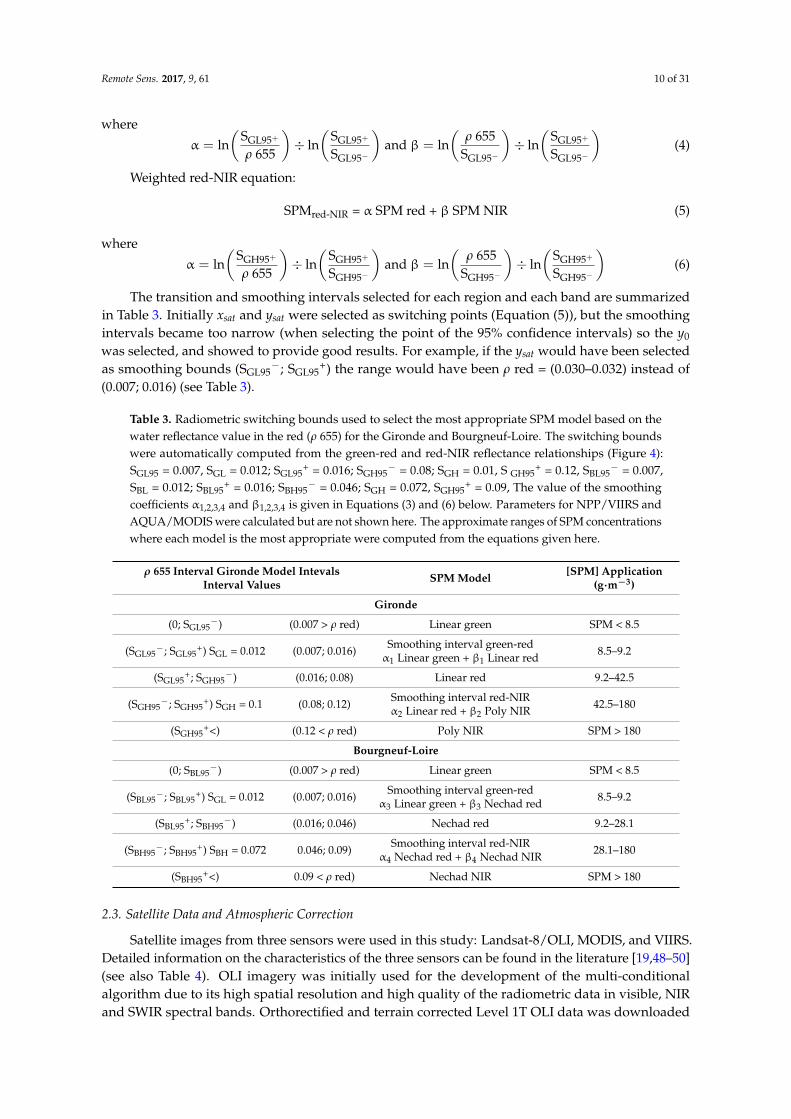
The transition and smoothing intervals selected for each region and each band are summarizedin Table 3. Initially xsat and ysat were selected as switching points (Equation (5)), but the smoothingintervals became too narrow (when selecting the point of the 95% confidence intervals) so the y0

was selected, and showed to provide good results. For example, if the ysat would have been selectedas smoothing bounds (SGL95

−; SGL95+) the range would have been ρ red = (0.030–0.032) instead of

(0.007; 0.016) (see Table 3).

Table 3. Radiometric switching bounds used to select the most appropriate SPM model based on thewater reflectance value in the red (ρ 655) for the Gironde and Bourgneuf-Loire. The switching boundswere automatically computed from the green-red and red-NIR reflectance relationships (Figure 4):SGL95 = 0.007, SGL = 0.012; SGL95

+ = 0.016; SGH95− = 0.08; SGH = 0.01, S GH95

+ = 0.12, SBL95− = 0.007,

SBL = 0.012; SBL95+ = 0.016; SBH95

− = 0.046; SGH = 0.072, SGH95+ = 0.09, The value of the smoothing

coefficients α1,2,3,4 and β1,2,3,4 is given in Equations (3) and (6) below. Parameters for NPP/VIIRS andAQUA/MODIS were calculated but are not shown here. The approximate ranges of SPM concentrationswhere each model is the most appropriate were computed from the equations given here.

ρ 655 Interval Gironde Model IntevalsInterval Values SPM Model [SPM] Application

(g·m−3)

Gironde

(0; SGL95−) (0.007 > ρ red) Linear green SPM < 8.5

(SGL95−; SGL95

+) SGL = 0.012 (0.007; 0.016) Smoothing interval green-redα1 Linear green + β1 Linear red 8.5–9.2

(SGL95+; SGH95

−) (0.016; 0.08) Linear red 9.2–42.5

(SGH95−; SGH95

+) SGH = 0.1 (0.08; 0.12) Smoothing interval red-NIRα2 Linear red + β2 Poly NIR 42.5–180

(SGH95+<) (0.12 < ρ red) Poly NIR SPM > 180

Bourgneuf-Loire

(0; SBL95−) (0.007 > ρ red) Linear green SPM < 8.5

(SBL95−; SBL95

+) SGL = 0.012 (0.007; 0.016) Smoothing interval green-redα3 Linear green + β3 Nechad red 8.5–9.2

(SBL95+; SBH95

−) (0.016; 0.046) Nechad red 9.2–28.1

(SBH95−; SBH95

+) SBH = 0.072 0.046; 0.09) Smoothing interval red-NIRα4 Nechad red + β4 Nechad NIR 28.1–180

(SBH95+<) 0.09 < ρ red) Nechad NIR SPM > 180

2.3. Satellite Data and Atmospheric Correction

Satellite images from three sensors were used in this study: Landsat-8/OLI, MODIS, and VIIRS.Detailed information on the characteristics of the three sensors can be found in the literature [19,48–50](see also Table 4). OLI imagery was initially used for the development of the multi-conditionalalgorithm due to its high spatial resolution and high quality of the radiometric data in visible, NIRand SWIR spectral bands. Orthorectified and terrain corrected Level 1T OLI data was downloaded

Remote Sens. 2017, 9, 61 11 of 31

from the Landsat-8 portal USGS portal (http://earthexplorer.usgs.gov/) then processed using theACOLITE software (http://odnature.naturalsciences.be/remsem/acolite-forum/) [19,51] to derivewater-leaving reflectance (hereinafter referred as ρw = π × Rrs). ACOLITE establishes a per-tile aerosoltype (or epsilon) as the ratio between the Rayleigh corrected reflectance in the aerosol correctionbands, for pixels where the marine reflectance can be assumed to be zero (where ρw 655 < 0.005,as defined by [19]. The epsilon is then used to extrapolate the observed aerosol reflectance to thevisible bands. ACOLITE also provides a choice for aerosol correction using a full tile fixed epsilon,a per pixel variable epsilon or a user defined epsilon. In this study, the first option was selected forthe atmospheric correction, as it has been shown to provide good results in highly turbid coastalwaters [52]. This software proposes two atmospheric correction (AC) options: the NIR algorithm [51]based on the MUMM approach [23] and using the red (655 nm) and NIR (865 nm) bands, and theSWIR algorithm [19] using the SWIR bands 6 (1609 nm) and 7 (2201 nm). Both atmospheric corrections(NIR and SWIR) were tested in the Gironde area. Four images for the Gironde and four for theBourgneuf-Loire areas were used for the NIR-SWIR atmospheric correction analysis. Then, the SWIRAC products were compared to the MACCS (Multisensor Atmospheric Correction and Cloud Screeningprocessor) product provided by the Theia Land Data Center (theia.cnes.fr), which was developedby [53]. Its innovation relies on the combination of a multi-spectral assumption that associates thesurface reflectance of the red and blue bands of the satellite, with the multi-temporal assumption thatobservations of a given region on land separated by a few days should yield similar surface reflectancevalues. They are also corrected for environmental effects. A total of 10 satellite images were used forthis ACOLITE-MACCS inter-comparison (Table 5) and to test the SPM multi-conditional algorithm.

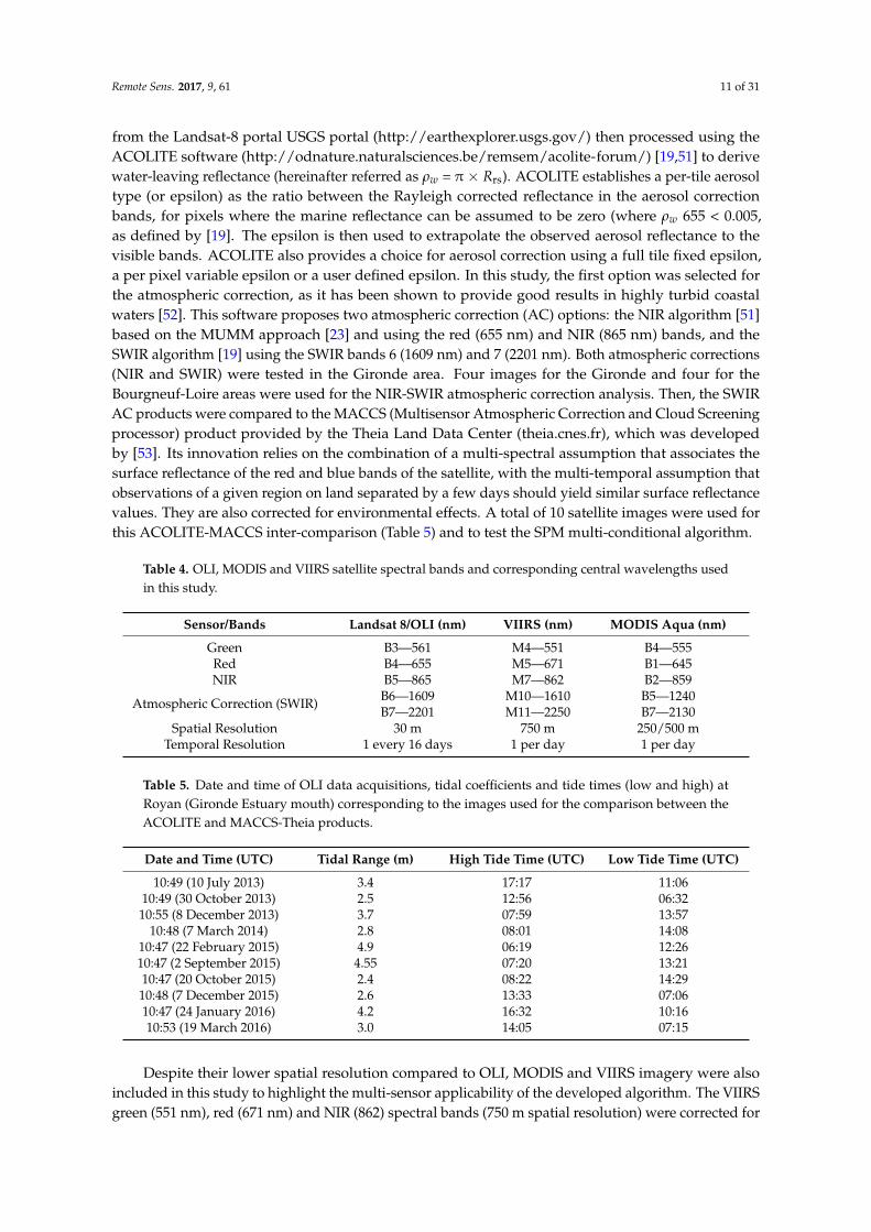
Table 4. OLI, MODIS and VIIRS satellite spectral bands and corresponding central wavelengths usedin this study.

Sensor/Bands Landsat 8/OLI (nm) VIIRS (nm) MODIS Aqua (nm)

Green B3—561 M4—551 B4—555Red B4—655 M5—671 B1—645NIR B5—865 M7—862 B2—859

Atmospheric Correction (SWIR) B6—1609 M10—1610 B5—1240B7—2201 M11—2250 B7—2130

Spatial Resolution 30 m 750 m 250/500 mTemporal Resolution 1 every 16 days 1 per day 1 per day

Table 5. Date and time of OLI data acquisitions, tidal coefficients and tide times (low and high) atRoyan (Gironde Estuary mouth) corresponding to the images used for the comparison between theACOLITE and MACCS-Theia products.

Date and Time (UTC) Tidal Range (m) High Tide Time (UTC) Low Tide Time (UTC)

10:49 (10 July 2013) 3.4 17:17 11:0610:49 (30 October 2013) 2.5 12:56 06:3210:55 (8 December 2013) 3.7 07:59 13:57

10:48 (7 March 2014) 2.8 08:01 14:0810:47 (22 February 2015) 4.9 06:19 12:2610:47 (2 September 2015) 4.55 07:20 13:2110:47 (20 October 2015) 2.4 08:22 14:2910:48 (7 December 2015) 2.6 13:33 07:0610:47 (24 January 2016) 4.2 16:32 10:1610:53 (19 March 2016) 3.0 14:05 07:15

Despite their lower spatial resolution compared to OLI, MODIS and VIIRS imagery were alsoincluded in this study to highlight the multi-sensor applicability of the developed algorithm. The VIIRSgreen (551 nm), red (671 nm) and NIR (862) spectral bands (750 m spatial resolution) were corrected for

Remote Sens. 2017, 9, 61 12 of 31

atmospheric effects using the Gordon and Wang approach in SeaDAS/l2gen (aeropt = −1) with bandsM10 (1610 nm) and M11 (2250) as aerosol correction bands. Unfortunately, SeaDAS/l2gen does notallow to process the two VIIRS high spatial resolution bands (I1 and I2, 375 m spatial resolution), so theproducts presented in this study were generated at a resolution of 250 m by interpolating the 750 mresolution bands (M4, M5, M7). The resulting VIIRS products were compared to OLI products and to insitu measurements carried out during the field campaigns. Then, the multi-conditional SPM algorithmwas applied to one image acquired over the Gironde area and another over the Bourgneuf-Loire area.This algorithm is also applied to MODIS (AQUA) images that were atmospherically corrected usingthe same atmospheric correction as VIIRS images, using the 1240 (B5) and 2130 nm (B7) MODIS SWIRbands. The band 1640 nm was not used due to the presence of faulty detectors on MODIS Aqua.This type of atmospheric correction was selected because it was shown to perform well in highlyturbid waters [52]. Reference [54] has shown that VIIRS performance is comparable to MODIS Aquain corresponding bands in all key performance regions of common spectral coverage, even if there arestill some VIIRS calibration issues [55].

Note that to generate satellite products, cloud masking was applied using a reflectance thresholdof 0.018 on the 2130 nm (OLI), 2250 nm (VIIRS) and 2130 nm (MODIS) wavebands, which avoidsmasking turbid waters.

2.4. Multi-Conditional SPM Algorithm Validation

Additional in situ turbidity measurements from the Gironde and Loire Estuary monitoringnetworks were used to validate the multi-conditional SPM algorithm through match-up withL8/OLI-derived SPM concentration. Due to their larger spatial resolution and the proximity of the insitu stations to the coast, MODIS and VIIRS data were not included in in situ—satellite match-ups.

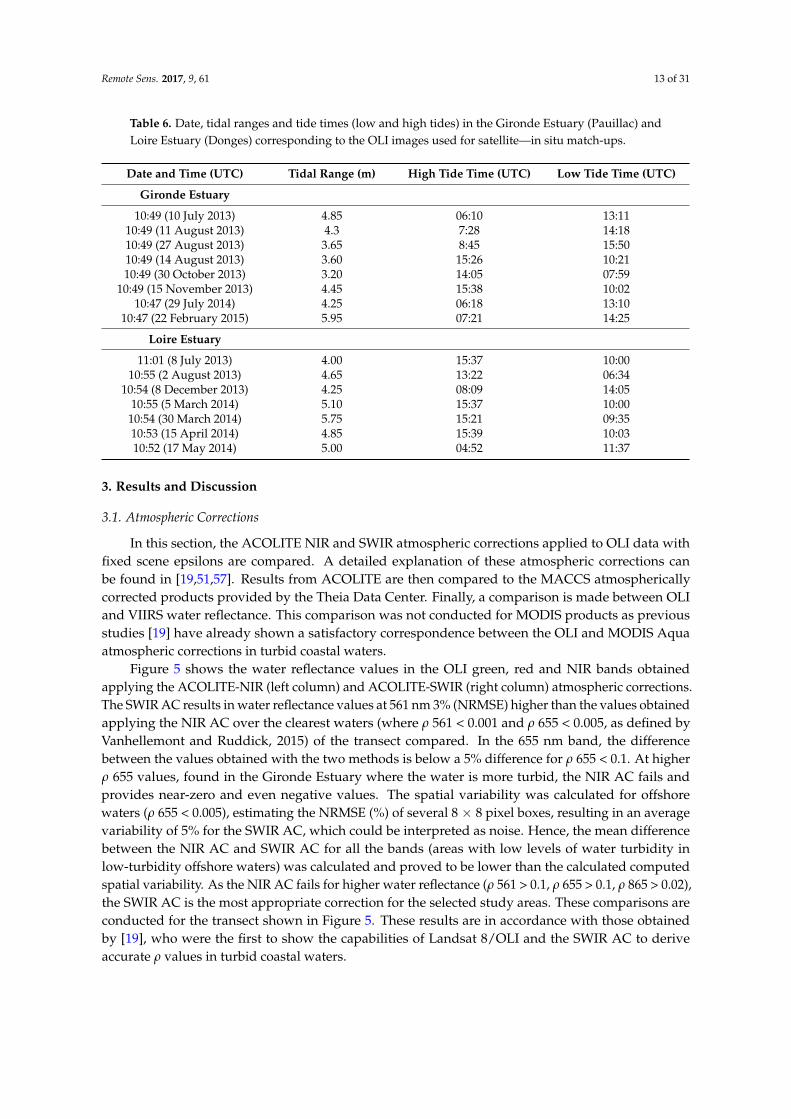
The Gironde Estuary includes an automated continuous monitoring network, called MAGEST(MArel Gironde ESTuary), [56] comprising four sites (Figure 2): Pauillac in the central Estuary (52 kmupstream the mouth); Libourne in the Dordogne tidal river (115 km upstream the mouth), and Bordeauxand Portets in the Garonne river (100 and 140 km upstream the mouth, respectively). The automatedstations record dissolved oxygen, temperature, turbidity and salinity every ten minutes at 1 m belowthe surface. Information on this network can be found at: http://www.magest.u-bordeaux1.fr/.The turbidity sensors (Endress and Hauser, CUS31-W2A) measure values between 0 and 9999 NTUwith a precision of 10%. Data from this station were selected within 10 min of the OLI overpasses.The temporal variability (standard deviation) was calculated for measurements conducted at thestations 30 min before and after the satellite overpass. The Loire Estuary also includes the same typeof monitoring stations (MAREL), which continuously carry out measurements at different locations.These measurements have been conducted since 2007 in the frame of the SYVEL (Système de veilledans l’estuaire de la Loire) monitoring network operated by the GIPLE (Groupement d’Intérêt PublicLoire Estuaire, Nantes, France). Information on the SYVEL network can be found at http://www.loire-estuaire.org/. As in the Gironde Estuary, the sensors are housed inside an instrumented chamber fixedon a pier, where the same type of measurements are recorded. In this study, we used data providedby two of the six stations in the Loire Estuary: the Paimboeuf and Donges stations (see locations onFigure 1). The SYVEL network provides turbidity data, which is then calibrated in SPM concentrationusing a regional relationship (GIPLE, 2014). In the case of the MAGEST network, turbidity wasconverted to SPM estimates using the relationship found in the Gironde. Different pixel configurationswere selected for the match-ups, for example, using the closest pixel to the MAREL station or anaverage of several pixels. Only the results obtained with the best method in each area (Gironde orLoire) are presented. The dates to the OLI images used for satellite—in situ match-ups are shown inTable 6, together with tidal ranges and tide times (low and high tides) in the Gironde Estuary (Pauillac)and Loire Estuary (Donges) at those dates.

Remote Sens. 2017, 9, 61 13 of 31

Table 6. Date, tidal ranges and tide times (low and high tides) in the Gironde Estuary (Pauillac) andLoire Estuary (Donges) corresponding to the OLI images used for satellite—in situ match-ups.

Date and Time (UTC) Tidal Range (m) High Tide Time (UTC) Low Tide Time (UTC)

Gironde Estuary

10:49 (10 July 2013) 4.85 06:10 13:1110:49 (11 August 2013) 4.3 7:28 14:1810:49 (27 August 2013) 3.65 8:45 15:5010:49 (14 August 2013) 3.60 15:26 10:2110:49 (30 October 2013) 3.20 14:05 07:59

10:49 (15 November 2013) 4.45 15:38 10:0210:47 (29 July 2014) 4.25 06:18 13:10

10:47 (22 February 2015) 5.95 07:21 14:25

Loire Estuary

11:01 (8 July 2013) 4.00 15:37 10:0010:55 (2 August 2013) 4.65 13:22 06:34

10:54 (8 December 2013) 4.25 08:09 14:0510:55 (5 March 2014) 5.10 15:37 10:00

10:54 (30 March 2014) 5.75 15:21 09:3510:53 (15 April 2014) 4.85 15:39 10:0310:52 (17 May 2014) 5.00 04:52 11:37

3. Results and Discussion

3.1. Atmospheric Corrections

In this section, the ACOLITE NIR and SWIR atmospheric corrections applied to OLI data withfixed scene epsilons are compared. A detailed explanation of these atmospheric corrections canbe found in [19,51,57]. Results from ACOLITE are then compared to the MACCS atmosphericallycorrected products provided by the Theia Data Center. Finally, a comparison is made between OLIand VIIRS water reflectance. This comparison was not conducted for MODIS products as previousstudies [19] have already shown a satisfactory correspondence between the OLI and MODIS Aquaatmospheric corrections in turbid coastal waters.

Figure 5 shows the water reflectance values in the OLI green, red and NIR bands obtainedapplying the ACOLITE-NIR (left column) and ACOLITE-SWIR (right column) atmospheric corrections.The SWIR AC results in water reflectance values at 561 nm 3% (NRMSE) higher than the values obtainedapplying the NIR AC over the clearest waters (where ρ 561 < 0.001 and ρ 655 < 0.005, as defined byVanhellemont and Ruddick, 2015) of the transect compared. In the 655 nm band, the differencebetween the values obtained with the two methods is below a 5% difference for ρ 655 < 0.1. At higherρ 655 values, found in the Gironde Estuary where the water is more turbid, the NIR AC fails andprovides near-zero and even negative values. The spatial variability was calculated for offshorewaters (ρ 655 < 0.005), estimating the NRMSE (%) of several 8 × 8 pixel boxes, resulting in an averagevariability of 5% for the SWIR AC, which could be interpreted as noise. Hence, the mean differencebetween the NIR AC and SWIR AC for all the bands (areas with low levels of water turbidity inlow-turbidity offshore waters) was calculated and proved to be lower than the calculated computedspatial variability. As the NIR AC fails for higher water reflectance (ρ 561 > 0.1, ρ 655 > 0.1, ρ 865 > 0.02),the SWIR AC is the most appropriate correction for the selected study areas. These comparisons areconducted for the transect shown in Figure 5. These results are in accordance with those obtainedby [19], who were the first to show the capabilities of Landsat 8/OLI and the SWIR AC to deriveaccurate ρ values in turbid coastal waters.

Remote Sens. 2017, 9, 61 14 of 31

Remote Sens. 2017, 9, 61 14 of 31

(a)

(b)

(c)

Figure 5. Comparison between NIR (left column) and SWIR (right column) atmospheric corrections applied to OLI data along a transect in the Gironde area on 7 March 2014. OLI bands at (a) 561 nm; (b) 655 nm; and (c) 865 nm (expressed as = × ) atmospherically corrected using the NIR and the SWIR options are shown. A transect (red line) over the plume and estuarine waters illustrates the comparison between the reflectance values derived using both atmospheric corrections.

3.1.1. ACOLITE vs. MACCS Products Comparison

Here, the ACOLITE SWIR AC and Theia Data Center MACCS water reflectance products are compared (Figure 6). The highest differences were observed over the less turbid waters, but in general a good agreement exists between both products. The flagged (grey) pixels on MACCS maps over the estuary correspond to the limit of the tile provided by the MACCS-Theia Land Data Center (longitude > 0°45′W). Figure 6b compares ρ values in the green, red and NIR bands obtained by applying both atmospheric corrections to the selected images (Table 5). The selected images were acquired at different periods of the year and for different tidal conditions. The best correlations were obtained for the red and the NIR bands with coefficients of determination of 0.95, a slope close to 1 and a NRMSE around 5%. The maximum differences were observed in the green band (NRMSE = ~7%).

Figure 5. Comparison between NIR (left column) and SWIR (right column) atmospheric correctionsapplied to OLI data along a transect in the Gironde area on 7 March 2014. OLI bands at (a) 561 nm;(b) 655 nm; and (c) 865 nm (expressed as ρ = Rrs × π) atmospherically corrected using the NIR andthe SWIR options are shown. A transect (red line) over the plume and estuarine waters illustrates thecomparison between the reflectance values derived using both atmospheric corrections.

3.1.1. ACOLITE vs. MACCS Products Comparison

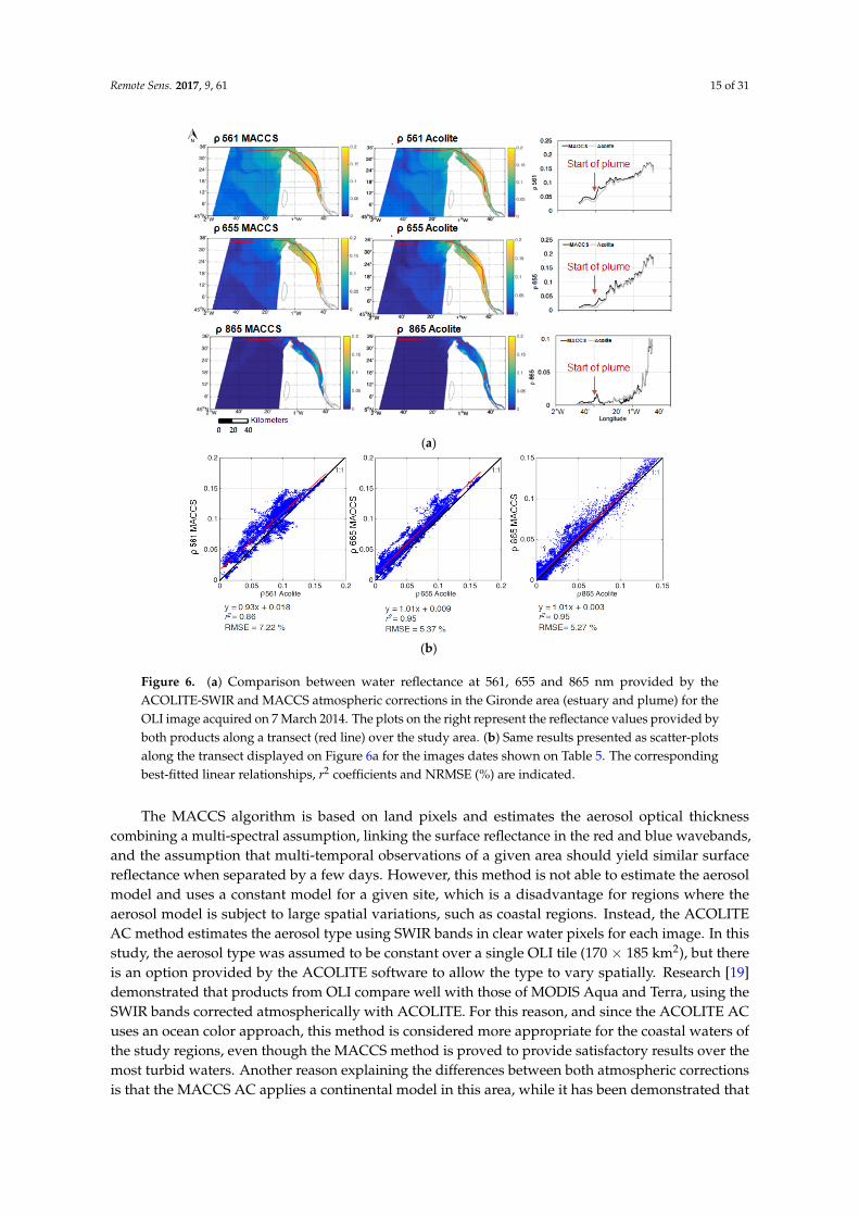
Here, the ACOLITE SWIR AC and Theia Data Center MACCS water reflectance products arecompared (Figure 6). The highest differences were observed over the less turbid waters, but in generala good agreement exists between both products. The flagged (grey) pixels on MACCS maps overthe estuary correspond to the limit of the tile provided by the MACCS-Theia Land Data Center(longitude > 0◦45′W). Figure 6b compares ρ values in the green, red and NIR bands obtained byapplying both atmospheric corrections to the selected images (Table 5). The selected images wereacquired at different periods of the year and for different tidal conditions. The best correlations wereobtained for the red and the NIR bands with coefficients of determination of 0.95, a slope close to 1 anda NRMSE around 5%. The maximum differences were observed in the green band (NRMSE = ~7%).

Remote Sens. 2017, 9, 61 15 of 31Remote Sens. 2017, 9, 61 15 of 31

(a)

(b)

Figure 6. (a) Comparison between water reflectance at 561, 655 and 865 nm provided by the ACOLITE-SWIR and MACCS atmospheric corrections in the Gironde area (estuary and plume) for the OLI image acquired on 7 March 2014. The plots on the right represent the reflectance values provided by both products along a transect (red line) over the study area. (b) Same results presented as scatter-plots along the transect displayed on Figure 6a for the images dates shown on Table 5. The corresponding best-fitted linear relationships, r2 coefficients and NRMSE (%) are indicated.

The MACCS algorithm is based on land pixels and estimates the aerosol optical thickness combining a multi-spectral assumption, linking the surface reflectance in the red and blue wavebands, and the assumption that multi-temporal observations of a given area should yield similar surface reflectance when separated by a few days. However, this method is not able to estimate the aerosol model and uses a constant model for a given site, which is a disadvantage for regions where the aerosol model is subject to large spatial variations, such as coastal regions. Instead, the ACOLITE AC method estimates the aerosol type using SWIR bands in clear water pixels for each image. In this study, the aerosol type was assumed to be constant over a single OLI tile (170 × 185 km2), but there is an option provided by the ACOLITE software to allow the type to vary spatially. Research [19] demonstrated that products from OLI compare well with those of MODIS Aqua and Terra, using the SWIR bands corrected atmospherically with ACOLITE. For this reason, and since the ACOLITE AC uses an ocean color approach, this method is considered more appropriate for the coastal waters of the study regions, even though the MACCS method is proved to provide satisfactory results over the most turbid waters. Another reason explaining the differences between both atmospheric corrections is that the MACCS AC applies a continental

Figure 6. (a) Comparison between water reflectance at 561, 655 and 865 nm provided by theACOLITE-SWIR and MACCS atmospheric corrections in the Gironde area (estuary and plume) for theOLI image acquired on 7 March 2014. The plots on the right represent the reflectance values provided byboth products along a transect (red line) over the study area. (b) Same results presented as scatter-plotsalong the transect displayed on Figure 6a for the images dates shown on Table 5. The correspondingbest-fitted linear relationships, r2 coefficients and NRMSE (%) are indicated.

The MACCS algorithm is based on land pixels and estimates the aerosol optical thicknesscombining a multi-spectral assumption, linking the surface reflectance in the red and blue wavebands,and the assumption that multi-temporal observations of a given area should yield similar surfacereflectance when separated by a few days. However, this method is not able to estimate the aerosolmodel and uses a constant model for a given site, which is a disadvantage for regions where theaerosol model is subject to large spatial variations, such as coastal regions. Instead, the ACOLITEAC method estimates the aerosol type using SWIR bands in clear water pixels for each image. In thisstudy, the aerosol type was assumed to be constant over a single OLI tile (170 × 185 km2), but thereis an option provided by the ACOLITE software to allow the type to vary spatially. Research [19]demonstrated that products from OLI compare well with those of MODIS Aqua and Terra, using theSWIR bands corrected atmospherically with ACOLITE. For this reason, and since the ACOLITE ACuses an ocean color approach, this method is considered more appropriate for the coastal waters ofthe study regions, even though the MACCS method is proved to provide satisfactory results over themost turbid waters. Another reason explaining the differences between both atmospheric correctionsis that the MACCS AC applies a continental model in this area, while it has been demonstrated that

Remote Sens. 2017, 9, 61 16 of 31

the maritime model is dominant in the Gironde area [58]. The aerosols of maritime origin are almostnon-absorbent, so an overestimation of aerosol absorbance is expected when applying a continentalmodel, especially in offshore waters where there is no land aerosol influence. The reason for the greenband differences observed is unclear; it could be due to an overestimation caused by the MACCS AC,or an underestimation by the ACOLITE AC caused by a green band overcorrection. However, as themajor differences are observed for the lower ρw values (Figure 6b), this dissimilarity is probably relatedto a flawed correction over offshore waters, where low green ρw values are usually found. Studiesfound on the use of the MACCS AC over coastal areas did not provide information that could explainthe differences observed [42,58] other than those already mentioned. Since the green band NRMSEpercentage remained low enough (<7%) for the purpose of this study, a deeper analysis on the reasonsfor these differences was considered out of scope.

3.1.2. Validation of Atmospheric Correction

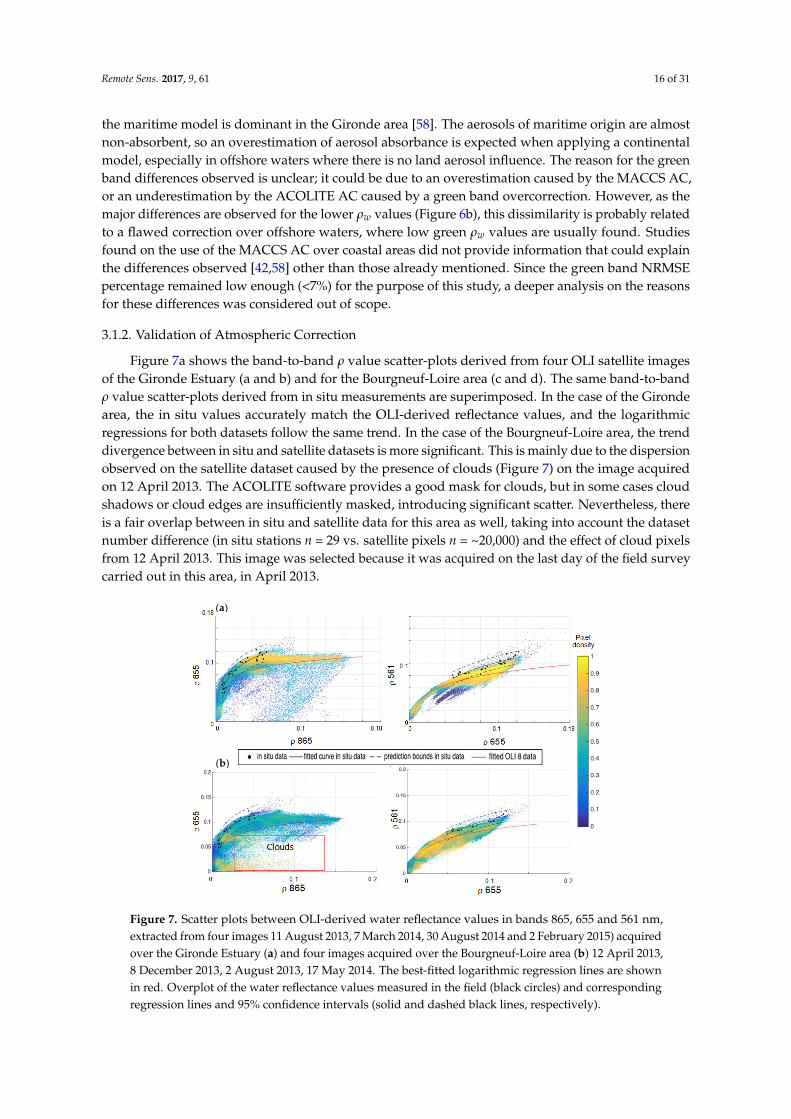
Figure 7a shows the band-to-band ρ value scatter-plots derived from four OLI satellite imagesof the Gironde Estuary (a and b) and for the Bourgneuf-Loire area (c and d). The same band-to-bandρ value scatter-plots derived from in situ measurements are superimposed. In the case of the Girondearea, the in situ values accurately match the OLI-derived reflectance values, and the logarithmicregressions for both datasets follow the same trend. In the case of the Bourgneuf-Loire area, the trenddivergence between in situ and satellite datasets is more significant. This is mainly due to the dispersionobserved on the satellite dataset caused by the presence of clouds (Figure 7) on the image acquiredon 12 April 2013. The ACOLITE software provides a good mask for clouds, but in some cases cloudshadows or cloud edges are insufficiently masked, introducing significant scatter. Nevertheless, thereis a fair overlap between in situ and satellite data for this area as well, taking into account the datasetnumber difference (in situ stations n = 29 vs. satellite pixels n = ~20,000) and the effect of cloud pixelsfrom 12 April 2013. This image was selected because it was acquired on the last day of the field surveycarried out in this area, in April 2013.

Remote Sens. 2017, 9, 61 16 of 31

model in this area, while it has been demonstrated that the maritime model is dominant in the Gironde area [58]. The aerosols of maritime origin are almost non-absorbent, so an overestimation of aerosol absorbance is expected when applying a continental model, especially in offshore waters where there is no land aerosol influence. The reason for the green band differences observed is unclear; it could be due to an overestimation caused by the MACCS AC, or an underestimation by the ACOLITE AC caused by a green band overcorrection. However, as the major differences are observed for the lower ρw values (Figure 6b), this dissimilarity is probably related to a flawed correction over offshore waters, where low green ρw values are usually found. Studies found on the use of the MACCS AC over coastal areas did not provide information that could explain the differences observed [42,58] other than those already mentioned. Since the green band NRMSE percentage remained low enough (<7%) for the purpose of this study, a deeper analysis on the reasons for these differences was considered out of scope.

3.1.2. Validation of Atmospheric Correction

Figure 7a shows the band-to-band ρ value scatter-plots derived from four OLI satellite images of the Gironde Estuary (a and b) and for the Bourgneuf-Loire area (c and d). The same band-to-band ρ value scatter-plots derived from in situ measurements are superimposed. In the case of the Gironde area, the in situ values accurately match the OLI-derived reflectance values, and the logarithmic regressions for both datasets follow the same trend. In the case of the Bourgneuf-Loire area, the trend divergence between in situ and satellite datasets is more significant. This is mainly due to the dispersion observed on the satellite dataset caused by the presence of clouds (Figure 7) on the image acquired on 12 April 2013. The ACOLITE software provides a good mask for clouds, but in some cases cloud shadows or cloud edges are insufficiently masked, introducing significant scatter. Nevertheless, there is a fair overlap between in situ and satellite data for this area as well, taking into account the dataset number difference (in situ stations n = 29 vs. satellite pixels n = ~20,000) and the effect of cloud pixels from 12 April 2013. This image was selected because it was acquired on the last day of the field survey carried out in this area, in April 2013.

Figure 7. Scatter plots between OLI-derived water reflectance values in bands 865, 655 and 561 nm, extracted from four images 11 August 2013, 7 March 2014, 30 August 2014 and 2 February 2015) acquired over the Gironde Estuary (a) and four images acquired over the Bourgneuf-Loire area (b) 12 April 2013, 8 December 2013, 2 August 2013, 17 May 2014. The best-fitted logarithmic regression lines are shown in red. Overplot of the water reflectance values measured in the field (black circles) and corresponding regression lines and 95% confidence intervals (solid and dashed black lines, respectively).

(a)

(b)

Figure 7. Scatter plots between OLI-derived water reflectance values in bands 865, 655 and 561 nm,extracted from four images 11 August 2013, 7 March 2014, 30 August 2014 and 2 February 2015) acquiredover the Gironde Estuary (a) and four images acquired over the Bourgneuf-Loire area (b) 12 April 2013,8 December 2013, 2 August 2013, 17 May 2014. The best-fitted logarithmic regression lines are shownin red. Overplot of the water reflectance values measured in the field (black circles) and correspondingregression lines and 95% confidence intervals (solid and dashed black lines, respectively).

Remote Sens. 2017, 9, 61 17 of 31

Similar ρ band-to-band comparisons were conducted between VIIRS-derived images, and insitu–measured water reflectance at bands centered at 551, 671 and 862 nm (Figure 8). A fair match isobtained between field and satellite datasets for both the Gironde and the Bourgneuf-Loire areas. As canbe observed, the in situ (black line) and satellite (red line) regression curves overlap. This demonstratesthat the atmospheric correction applied to the VIIRS images, using the SWIR bands and the Seadas(version 7.3), is appropriate for this type of environment.

Remote Sens. 2017, 9, 61 17 of 31

Similar ρ band-to-band comparisons were conducted between VIIRS-derived images, and in situ–measured water reflectance at bands centered at 551, 671 and 862 nm (Figure 8). A fair match is obtained between field and satellite datasets for both the Gironde and the Bourgneuf-Loire areas. As can be observed, the in situ (black line) and satellite (red line) regression curves overlap. This demonstrates that the atmospheric correction applied to the VIIRS images, using the SWIR bands and the Seadas (version 7.3), is appropriate for this type of environment.

Figure 8. Scatter plots between VIIRS-derived water reflectance values at 862, 671 and 551 (862 vs. 671 and 671 vs. 551) extracted from the image acquired on 7 March 2014 over the Gironde Estuary (a) and over Bourgneuf Bay and the Loire Estuary on 12 April 2013 (b) and atmospherically corrected using the SWIR bands. The fitted logarithmic regression line of the satellite data is shown in red, the in situ data acquired during the field campaign conducted in 2013 is represented using black dots; the regression line fitted to the in situ data and the 95% confidence intervals are shown, respectively, as solid and dashed black lines.

Figure 9 presents a comparison between in situ–measured and satellite-derived reflectance spectra corresponding to VIIRS and MODIS Aqua images acquired on 12 June 2012, 15 July 2014, 16 July 2014.. Satellite data were atmospherically corrected using the SWIR option as well. A good match was obtained for the plume area, but in the estuary, the satellite-derived reflectance was systematically lower than values measured in situ at the Pauillac station. This is due to the size sampling differences (satellite vs. in situ) and the effect of the land reflectance in land/water border pixels. Water pixels located near the shore may be contaminated by the land signal, causing erroneous water reflectance estimates. This underestimation in the case of VIIRS (Figure 9a) is lower than in the case of MODIS, where a particularly sudden decrease is observed for the lower wavelengths. This is caused by the use of the MODIS band B5 (1240 nm), which causes an overcorrection in the shorter wavelength band.

(a)

(b)

Figure 8. Scatter plots between VIIRS-derived water reflectance values at 862, 671 and 551 (862 vs. 671and 671 vs. 551) extracted from the image acquired on 7 March 2014 over the Gironde Estuary (a) andover Bourgneuf Bay and the Loire Estuary on 12 April 2013 (b) and atmospherically corrected using theSWIR bands. The fitted logarithmic regression line of the satellite data is shown in red, the in situ dataacquired during the field campaign conducted in 2013 is represented using black dots; the regressionline fitted to the in situ data and the 95% confidence intervals are shown, respectively, as solid anddashed black lines.

Figure 9 presents a comparison between in situ–measured and satellite-derived reflectance spectracorresponding to VIIRS and MODIS Aqua images acquired on 12 June 2012, 15 July 2014, 16 July2014. Satellite data were atmospherically corrected using the SWIR option as well. A good match wasobtained for the plume area, but in the estuary, the satellite-derived reflectance was systematicallylower than values measured in situ at the Pauillac station. This is due to the size sampling differences(satellite vs. in situ) and the effect of the land reflectance in land/water border pixels. Water pixelslocated near the shore may be contaminated by the land signal, causing erroneous water reflectanceestimates. This underestimation in the case of VIIRS (Figure 9a) is lower than in the case of MODIS,where a particularly sudden decrease is observed for the lower wavelengths. This is caused by the useof the MODIS band B5 (1240 nm), which causes an overcorrection in the shorter wavelength band.

Remote Sens. 2017, 9, 61 18 of 31Remote Sens. 2017, 9, 61 18 of 31

(a) (b)

(c)

Figure 9. (a) Water reflectance spectra (ρ) measured in the field (12 June 2012, 15 July 2014, 16 July 2014) compared to VIIRS-derived (a) and MODIS-derived (b) water reflectance in the Gironde plume (grey lines) and estuary (black lines). (c) Location of the stations on the ρ 862 VIIRS map. There was a maximum time difference of 20 min between the in situ and the satellite data.

In Figure 10, the reflectance spectra measured in situ on 11 April 2016 at 10:26 (Station 1) and at 11:16 (Station 2) are compared to the OLI-derived values (image acquired at 10:53). There is a closer match between the water reflectance values measured at Station 2 than at Station 1. This could be due to the lower time difference between the image acquisition and the in situ measurement for Station 2 (23 min) than for Station 1 (27 min), together with the significant small-scale variability of the SPM concentration in this specific area given that measurements were conducted during the ebb tide. In general, satellite products appear to underestimate the ‘true’, i.e., field-measured, water reflectance. Valid match-ups with MODIS and VIIRS were not obtained on the same day.

The comparison between in situ and satellite data products resulted in a good match between the green-red and red-NIR bands, with some discrepancies. In general, the trends observed for the satellite data were lower in the higher reflectance values. This is due to the difference in the amount of data (in situ stations n = 29 vs. satellite pixels n = ~20,000) and to cloud shadow and land effects on coastal pixels. Regarding the OLI red-green bands’ (655 vs. 561 nm) comparison, a break was observed between the 0–0.15 and the 0.15–0.2 intervals. If the fit would have been made for values of ρ 655 <0.08, the red and black curves in Figures 7 and 8 would have had a better correspondence for the lower reflectance values, so better results would have been obtained if the comparison was achieved by intervals (e.g., 0–0.08, 0.8–0.2). However, showing the entire data range provides a better understanding of the type of data obtained in situ and from satellite remote sensing measurements, and since the in situ data matches the satellite data, the atmospheric correction was

Figure 9. (a) Water reflectance spectra (ρ) measured in the field (12 June 2012, 15 July 2014, 16 July 2014)compared to VIIRS-derived (a) and MODIS-derived (b) water reflectance in the Gironde plume(grey lines) and estuary (black lines). (c) Location of the stations on the ρ 862 VIIRS map. There was amaximum time difference of 20 min between the in situ and the satellite data.

In Figure 10, the reflectance spectra measured in situ on 11 April 2016 at 10:26 (Station 1) andat 11:16 (Station 2) are compared to the OLI-derived values (image acquired at 10:53). There is acloser match between the water reflectance values measured at Station 2 than at Station 1. This couldbe due to the lower time difference between the image acquisition and the in situ measurement forStation 2 (23 min) than for Station 1 (27 min), together with the significant small-scale variability of theSPM concentration in this specific area given that measurements were conducted during the ebb tide.In general, satellite products appear to underestimate the ‘true’, i.e., field-measured, water reflectance.Valid match-ups with MODIS and VIIRS were not obtained on the same day.

The comparison between in situ and satellite data products resulted in a good match betweenthe green-red and red-NIR bands, with some discrepancies. In general, the trends observed for thesatellite data were lower in the higher reflectance values. This is due to the difference in the amountof data (in situ stations n = 29 vs. satellite pixels n = ~20,000) and to cloud shadow and land effectson coastal pixels. Regarding the OLI red-green bands’ (655 vs. 561 nm) comparison, a break wasobserved between the 0–0.15 and the 0.15–0.2 intervals. If the fit would have been made for valuesof ρ 655 <0.08, the red and black curves in Figures 7 and 8 would have had a better correspondencefor the lower reflectance values, so better results would have been obtained if the comparison wasachieved by intervals (e.g., 0–0.08, 0.8–0.2). However, showing the entire data range provides a better

Remote Sens. 2017, 9, 61 19 of 31

understanding of the type of data obtained in situ and from satellite remote sensing measurements,and since the in situ data matches the satellite data, the atmospheric correction was considered toprovide realistic reflectance results. The switching bounds were determined using field data, so a bettermatch between the two types of data (in situ vs. satellite) would not affect the switching boundvalues selected.

Remote Sens. 2017, 9, 61 19 of 31

considered to provide realistic reflectance results. The switching bounds were determined using field data, so a better match between the two types of data (in situ vs. satellite) would not affect the switching bound values selected.

Figure 10. (a) Water reflectance spectra (ρ) measured in situ in the Loire Estuary on 11 April 2016 compared to OLI-derived ρ values (SAT); (b) Location of the stations on the ρ 865 OLI map. There was a maximum time difference of 20 min between the in situ and the satellite data.

Differences observed between in situ and satellite data, in Figures 9 and 10, could be due to several reasons: (1) an overcorrection of the atmospheric contribution in the SWIR method; (2) the spatial difference between the satellite pixel and field measurements (250/750 m2 pixel versus ~1 m2); (3) the near-shore location of the station in the estuary. Option 3 appears to be the most plausible, as the pixel selected for the comparison did not correspond exactly to the location of the Pauillac field station: the next pixel away from the shore was selected to avoid the land effect. Thus, the reflectance values at this location are different to the ones measured in situ at Pauillac. In the case of MODIS (Figure 9b), there is an obvious overcorrection inside the estuary, due most probably to the low pixel resolution for this area combined with the selection of the 1240 SWIR band. This effect was also observed in the highly turbid waters of the La Plata river by [52].

3.2. OLI-VIIRS Comparison

Water reflectance values in the green, red and NIR OLI bands (561, 655 and 865 nm) were re-sampled by neighborhood, averaged to a grid of 750 m resolution and then compared to VIIRS-derived values at 551, 671 and 862 nm bands using a common grid. This comparison was achieved for the image acquired on 12 April 2013 (Table 7). A fair correspondence was found in the Gironde area for this cloud-free image with a large range of water reflectance values, taking into account the significant overpass time difference between both sensors (~3 h) and the large tidal dynamics occurring in this region, as well as the bandwidth differences between the two satellite sensors. The best correspondence was obtained in the green bands (slope = 0.83, r2 = 0.71), followed

(a)

(b)

Figure 10. (a) Water reflectance spectra (ρ) measured in situ in the Loire Estuary on 11 April 2016compared to OLI-derived ρ values (SAT); (b) Location of the stations on the ρ 865 OLI map. There wasa maximum time difference of 20 min between the in situ and the satellite data.

Differences observed between in situ and satellite data, in Figures 9 and 10, could be due to severalreasons: (1) an overcorrection of the atmospheric contribution in the SWIR method; (2) the spatialdifference between the satellite pixel and field measurements (250/750 m2 pixel versus ~1 m2);(3) the near-shore location of the station in the estuary. Option 3 appears to be the most plausible, as thepixel selected for the comparison did not correspond exactly to the location of the Pauillac field station:the next pixel away from the shore was selected to avoid the land effect. Thus, the reflectance values atthis location are different to the ones measured in situ at Pauillac. In the case of MODIS (Figure 9b),there is an obvious overcorrection inside the estuary, due most probably to the low pixel resolutionfor this area combined with the selection of the 1240 SWIR band. This effect was also observed in thehighly turbid waters of the La Plata river by [52].

3.2. OLI-VIIRS Comparison

Water reflectance values in the green, red and NIR OLI bands (561, 655 and 865 nm) werere-sampled by neighborhood, averaged to a grid of 750 m resolution and then compared toVIIRS-derived values at 551, 671 and 862 nm bands using a common grid. This comparison wasachieved for the image acquired on 12 April 2013 (Table 7). A fair correspondence was found in

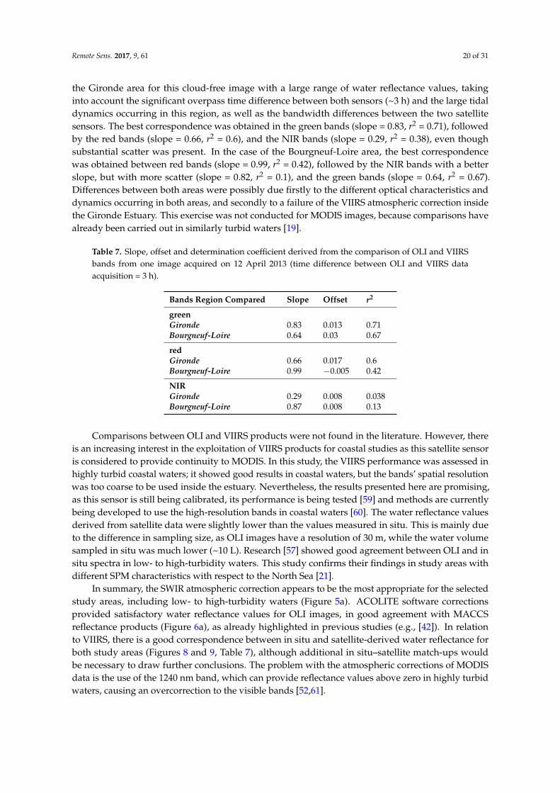
Remote Sens. 2017, 9, 61 20 of 31

the Gironde area for this cloud-free image with a large range of water reflectance values, takinginto account the significant overpass time difference between both sensors (~3 h) and the large tidaldynamics occurring in this region, as well as the bandwidth differences between the two satellitesensors. The best correspondence was obtained in the green bands (slope = 0.83, r2 = 0.71), followedby the red bands (slope = 0.66, r2 = 0.6), and the NIR bands (slope = 0.29, r2 = 0.38), even thoughsubstantial scatter was present. In the case of the Bourgneuf-Loire area, the best correspondencewas obtained between red bands (slope = 0.99, r2 = 0.42), followed by the NIR bands with a betterslope, but with more scatter (slope = 0.82, r2 = 0.1), and the green bands (slope = 0.64, r2 = 0.67).Differences between both areas were possibly due firstly to the different optical characteristics anddynamics occurring in both areas, and secondly to a failure of the VIIRS atmospheric correction insidethe Gironde Estuary. This exercise was not conducted for MODIS images, because comparisons havealready been carried out in similarly turbid waters [19].

Table 7. Slope, offset and determination coefficient derived from the comparison of OLI and VIIRSbands from one image acquired on 12 April 2013 (time difference between OLI and VIIRS dataacquisition = 3 h).

Bands Region Compared Slope Offset r2

greenGironde 0.83 0.013 0.71Bourgneuf-Loire 0.64 0.03 0.67

redGironde 0.66 0.017 0.6Bourgneuf-Loire 0.99 −0.005 0.42

NIRGironde 0.29 0.008 0.038Bourgneuf-Loire 0.87 0.008 0.13

Comparisons between OLI and VIIRS products were not found in the literature. However, thereis an increasing interest in the exploitation of VIIRS products for coastal studies as this satellite sensoris considered to provide continuity to MODIS. In this study, the VIIRS performance was assessed inhighly turbid coastal waters; it showed good results in coastal waters, but the bands’ spatial resolutionwas too coarse to be used inside the estuary. Nevertheless, the results presented here are promising,as this sensor is still being calibrated, its performance is being tested [59] and methods are currentlybeing developed to use the high-resolution bands in coastal waters [60]. The water reflectance valuesderived from satellite data were slightly lower than the values measured in situ. This is mainly dueto the difference in sampling size, as OLI images have a resolution of 30 m, while the water volumesampled in situ was much lower (~10 L). Research [57] showed good agreement between OLI and insitu spectra in low- to high-turbidity waters. This study confirms their findings in study areas withdifferent SPM characteristics with respect to the North Sea [21].

In summary, the SWIR atmospheric correction appears to be the most appropriate for the selectedstudy areas, including low- to high-turbidity waters (Figure 5a). ACOLITE software correctionsprovided satisfactory water reflectance values for OLI images, in good agreement with MACCSreflectance products (Figure 6a), as already highlighted in previous studies (e.g., [42]). In relationto VIIRS, there is a good correspondence between in situ and satellite-derived water reflectance forboth study areas (Figures 8 and 9, Table 7), although additional in situ–satellite match-ups wouldbe necessary to draw further conclusions. The problem with the atmospheric corrections of MODISdata is the use of the 1240 nm band, which can provide reflectance values above zero in highly turbidwaters, causing an overcorrection to the visible bands [52,61].

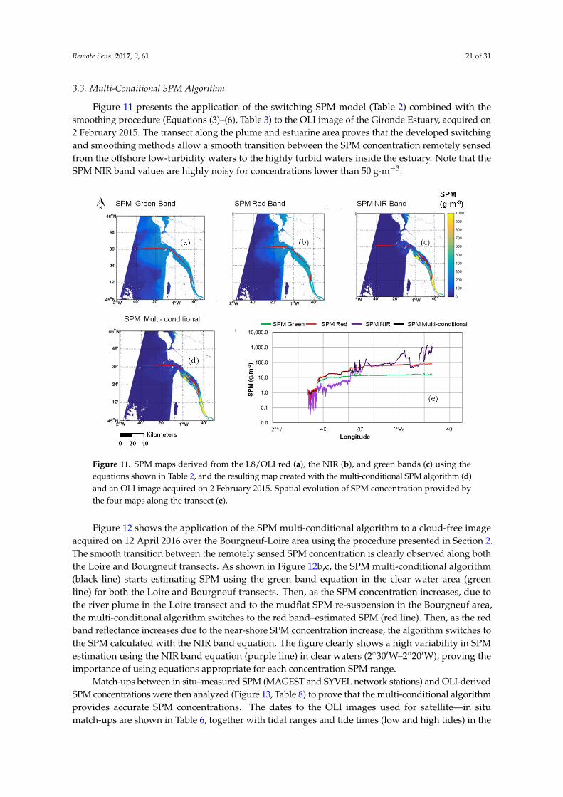
Remote Sens. 2017, 9, 61 21 of 31

3.3. Multi-Conditional SPM Algorithm

Figure 11 presents the application of the switching SPM model (Table 2) combined with thesmoothing procedure (Equations (3)–(6), Table 3) to the OLI image of the Gironde Estuary, acquired on2 February 2015. The transect along the plume and estuarine area proves that the developed switchingand smoothing methods allow a smooth transition between the SPM concentration remotely sensedfrom the offshore low-turbidity waters to the highly turbid waters inside the estuary. Note that theSPM NIR band values are highly noisy for concentrations lower than 50 g·m−3.Remote Sens. 2017, 9, 61 21 of 31

Figure 11. SPM maps derived from the L8/OLI red (a), the NIR (b), and green bands (c) using the equations shown in Table 2, and the resulting map created with the multi-conditional SPM algorithm (d) and an OLI image acquired on 2 February 2015. Spatial evolution of SPM concentration provided by the four maps along the transect (e).

Figure 12 shows the application of the SPM multi-conditional algorithm to a cloud-free image acquired on 12 April 2016 over the Bourgneuf-Loire area using the procedure presented in Section 2. The smooth transition between the remotely sensed SPM concentration is clearly observed along both the Loire and Bourgneuf transects. As shown in Figure 12b,c, the SPM multi-conditional algorithm (black line) starts estimating SPM using the green band equation in the clear water area (green line) for both the Loire and Bourgneuf transects. Then, as the SPM concentration increases, due to the river plume in the Loire transect and to the mudflat SPM re-suspension in the Bourgneuf area, the multi-conditional algorithm switches to the red band–estimated SPM (red line). Then, as the red band reflectance increases due to the near-shore SPM concentration increase, the algorithm switches to the SPM calculated with the NIR band equation. The figure clearly shows a high variability in SPM estimation using the NIR band equation (purple line) in clear waters (2°30′W–2°20′W), proving the importance of using equations appropriate for each concentration SPM range.

Match-ups between in situ–measured SPM (MAGEST and SYVEL network stations) and OLI-derived SPM concentrations were then analyzed (Figure 13, Table 8) to prove that the multi-conditional algorithm provides accurate SPM concentrations. The dates to the OLI images used for satellite—in situ match-ups are shown in Table 6, together with tidal ranges and tide times (low and high tides) in the Gironde Estuary (Pauillac) and Loire Estuary (Donges) at those dates. The in situ SPM concentrations for the Gironde Estuary were derived from the turbidity measurements (in FNU) at the stations and the turbidity-SPM relationship was established with in situ measurements taken in the Gironde Estuary. In general, OLI provided good SPM estimates at the Pauillac and Libourne stations (r2 = 0.8 and 0.95, NMRSE = 16% and 14%, respectively, for Gironde and Loire). Previous match-ups using the MAGEST network measurements and SPOT 5 satellite data provided good results with higher pixel resolutions than OLI, showing the capacity of these stations for satellite imagery validation [42]. Additionally, the SPM concentration calculated using different models (refer to Table A2 in the appendix), including the models of

Figure 11. SPM maps derived from the L8/OLI red (a), the NIR (b), and green bands (c) using theequations shown in Table 2, and the resulting map created with the multi-conditional SPM algorithm (d)and an OLI image acquired on 2 February 2015. Spatial evolution of SPM concentration provided bythe four maps along the transect (e).

Figure 12 shows the application of the SPM multi-conditional algorithm to a cloud-free imageacquired on 12 April 2016 over the Bourgneuf-Loire area using the procedure presented in Section 2.The smooth transition between the remotely sensed SPM concentration is clearly observed along boththe Loire and Bourgneuf transects. As shown in Figure 12b,c, the SPM multi-conditional algorithm(black line) starts estimating SPM using the green band equation in the clear water area (greenline) for both the Loire and Bourgneuf transects. Then, as the SPM concentration increases, due tothe river plume in the Loire transect and to the mudflat SPM re-suspension in the Bourgneuf area,the multi-conditional algorithm switches to the red band–estimated SPM (red line). Then, as the redband reflectance increases due to the near-shore SPM concentration increase, the algorithm switches tothe SPM calculated with the NIR band equation. The figure clearly shows a high variability in SPMestimation using the NIR band equation (purple line) in clear waters (2◦30′W–2◦20′W), proving theimportance of using equations appropriate for each concentration SPM range.

Match-ups between in situ–measured SPM (MAGEST and SYVEL network stations) and OLI-derivedSPM concentrations were then analyzed (Figure 13, Table 8) to prove that the multi-conditional algorithmprovides accurate SPM concentrations. The dates to the OLI images used for satellite—in situmatch-ups are shown in Table 6, together with tidal ranges and tide times (low and high tides) in the

Remote Sens. 2017, 9, 61 22 of 31

Gironde Estuary (Pauillac) and Loire Estuary (Donges) at those dates. The in situ SPM concentrationsfor the Gironde Estuary were derived from the turbidity measurements (in FNU) at the stations and theturbidity-SPM relationship was established with in situ measurements taken in the Gironde Estuary.In general, OLI provided good SPM estimates at the Pauillac and Libourne stations (r2 = 0.8 and 0.95,NMRSE = 16% and 14%, respectively, for Gironde and Loire). Previous match-ups using the MAGESTnetwork measurements and SPOT 5 satellite data provided good results with higher pixel resolutionsthan OLI, showing the capacity of these stations for satellite imagery validation [42]. Additionally,the SPM concentration calculated using different models (refer to Table A2 in the appendix), includingthe models of [18,42], were matched to in situ SPM measurements. The resulting match-ups (Table 8)show that the multi-conditional algorithm provided, for both the Gironde and the Loire areas, the bestof fit (r2 = 0.8, 0.67) and low error (16%, 14%) combination when compared to SPM estimated usingother models. The combination of several models adapted to each concentration range is the mainreason for this result, together with the selection of the best-fitted models. As proved by otherstudies [35–37], the selection of a specific model combining different bands is an improvement whenestimating the SPM concentration in coastal waters.

Remote Sens. 2017, 9, 61 22 of 31

[18,42], were matched to in situ SPM measurements. The resulting match-ups (Table 8) show that the multi-conditional algorithm provided, for both the Gironde and the Loire areas, the best of fit (r2 = 0.8, 0.67) and low error (16%, 14%) combination when compared to SPM estimated using other models. The combination of several models adapted to each concentration range is the main reason for this result, together with the selection of the best-fitted models. As proved by other studies [35–37], the selection of a specific model combining different bands is an improvement when estimating the SPM concentration in coastal waters.

(b)

(a) (c)

Figure 12. (a) SPM map of the Bourgneuf Bay and Loire Estuary derived from OLI satellite image acquired on 12 April 2016 applying the SPM multi-conditional algorithm. The image was atmospherically corrected using the SWIR option of the ACOLITE software. Resulting SPM concentration transects along the Loire Estuary (b) and Bourgneuf Bay (c) retrieved using the three SPM single-band models (green, red and NIR bands) and with the multi-conditional algorithm.

Table 8 shows the in situ-satellite match-up results using different SPM models. In the case of the Gironde area, the fit, slope, NRMSE (%) and offset when using the band-ratio and single-band exponential and polynomial regressions were similar. Slightly better results were obtained with the exponential NIR-red band ratio models (r2 = 0.7, slope = 1.1, NRMSE = 22.3%, offset = 16) compared to the exponential NIR band model (r2 = 0.8, slope = 0.65, NRMSE = 20%, offset = 66), but the polynomial single-band model performed better when using the single NIR band (r2 = 0.8, slope = 0.8, NRMSE = 16.4%, offset = −3), compared to the band ratio (r2 = 0.74, slope = 0.9, NRMSE = 19.8%, offset = 33). The SPM concentration estimates did not improve when using equations published in other studies for the same study areas [18,42] providing larger NMRSEs (36.5%, 44.7%) and offsets (−185, −24), compared to the results obtained with the multi-conditional algorithm (slope = 0.8, r2 = 0.8, NRMSE = 16%, offset = −1.8). In the case of the Bourgneuf-Loire area, the combination of the re-calibrated NIR and red band semi-empirical models from Reference [16] with the multi-conditional algorithm provided the best fit and lowest error (slope = 0.67, r2 = 0.95, NRMSE = 14%, offset = 121). In this case, the performance of the algorithm will improve with a re-calibration of the models with additional in situ data.

The configuration of the pixels selected for the match-ups is shown in Figure 13. OLI-derived SPM estimates provided good match-up results with the in situ measurements. In the case of the Bourgneuf-Loire area, instead of using one pixel for the match-ups, as in the case of Gironde, an average of four pixels was used, as it provided the best results. Vertical error bars show the standard deviation of the four pixels selected, in the case of the Loire area (see Figure 13b), and of the three nearby pixels in the case of the Gironde area (shown as red rectangles), even if a single

Figure 12. (a) SPM map of the Bourgneuf Bay and Loire Estuary derived from OLI satellite image acquiredon 12 April 2016 applying the SPM multi-conditional algorithm. The image was atmospherically correctedusing the SWIR option of the ACOLITE software. Resulting SPM concentration transects along theLoire Estuary (b) and Bourgneuf Bay (c) retrieved using the three SPM single-band models (green, redand NIR bands) and with the multi-conditional algorithm.

Table 8 shows the in situ-satellite match-up results using different SPM models. In the case ofthe Gironde area, the fit, slope, NRMSE (%) and offset when using the band-ratio and single-bandexponential and polynomial regressions were similar. Slightly better results were obtained with theexponential NIR-red band ratio models (r2 = 0.7, slope = 1.1, NRMSE = 22.3%, offset = 16) comparedto the exponential NIR band model (r2 = 0.8, slope = 0.65, NRMSE = 20%, offset = 66), but thepolynomial single-band model performed better when using the single NIR band (r2 = 0.8, slope = 0.8,NRMSE = 16.4%, offset = −3), compared to the band ratio (r2 = 0.74, slope = 0.9, NRMSE = 19.8%,offset = 33). The SPM concentration estimates did not improve when using equations published inother studies for the same study areas [18,42] providing larger NMRSEs (36.5%, 44.7%) and offsets(−185, −24), compared to the results obtained with the multi-conditional algorithm (slope = 0.8,r2 = 0.8, NRMSE = 16%, offset = −1.8). In the case of the Bourgneuf-Loire area, the combination of there-calibrated NIR and red band semi-empirical models from Reference [16] with the multi-conditional

Remote Sens. 2017, 9, 61 23 of 31

algorithm provided the best fit and lowest error (slope = 0.67, r2 = 0.95, NRMSE = 14%, offset = 121).In this case, the performance of the algorithm will improve with a re-calibration of the models withadditional in situ data.

The configuration of the pixels selected for the match-ups is shown in Figure 13. OLI-derivedSPM estimates provided good match-up results with the in situ measurements. In the case of theBourgneuf-Loire area, instead of using one pixel for the match-ups, as in the case of Gironde, an averageof four pixels was used, as it provided the best results. Vertical error bars show the standard deviationof the four pixels selected, in the case of the Loire area (see Figure 13b), and of the three nearby pixelsin the case of the Gironde area (shown as red rectangles), even if a single pixel was used for thematch-ups (red circle) in Figure 13c. Horizontal error bars correspond to the temporal SPM variability±10 min from the satellite overpass time. There appears to be an underestimation by the algorithmat SPM concentrations above 100 g·m−3 and a slight overestimation below 500 g·m−3 (and above100 g·m−3) in the Bourgneuf-Loire area, while the Gironde algorithm seems to overestimate valuesabove 500 g·m−3. This tendency was also observed by [42] using SPOT 4 data, where the same pixelconfiguration was used for the Loire match-ups. The imprecision observed for these match-ups isdue to several factors, such as the accuracy of the SPM algorithms, the errors and uncertainties infield measurements, the spatial differences between the sampling station and satellite pixel location,as well as uncertainties related to atmospheric corrections. Different SPM models including bandratios, such as those developed by [18,42] for these areas, were applied to the images, but the match-upresults did not improve (see Table 8).

Figure 14 compares the SPM concentrations derived from OLI, VIIRS and MODIS (Aqua) satellitedata recorded on the same day over the Gironde Estuary. Water reflectances at 655 (OLI), 671 (VIIRS),645 nm (MODIS aqua) show a similar trend along the transect. VIIRS products provided higher valuesthan OLI in general, up to the most upstream section of the Estuary, where there was a sharp decrease.It corresponded to a failure of the atmospheric correction, due to the low VIIRS spatial resolutionfor this particular area. This failure was also observed along the MODIS transect, where the mostupstream pixels are missing, resulting in a sudden SPM concentration decrease. Generally, the MODISand OLI transects overlap up to the most upstream section of the estuary, where SPM concentrationsare overestimated by MODIS. This is due to the proximity of the land on the last transect pixels, which,as seen in Figure 13d, results in a rapid decrease of the SPM concentration. In this particular region,the reflectance at 859 nm showed a fast increase for MODIS, which was not observed in the OLI 865band. Hence, particular attention needs to be paid to the near-shore pixels, where the atmosphericcorrection may provide inaccurate water reflectance estimates, resulting in inaccurate SPM retrievals.For practical reasons, the same switching bounds applied to OLI were used for VIIRS and MODIS Aqua.However, the fine adjustment of the switching bounds to each sensor’s spectral bands could providebetter results. Despite the fact that the MODIS atmospheric corrections provided underestimatedwater reflectance values, the transect comparison showed a good match between the three SPM maps.

Overall, the multi-conditional SPM algorithm provides a smooth transition between SPMmodels for three different sensors over an area that goes from low- to high-turbidity surface waters.The band-switching technique allows keeping the optimal sensitivity of ρ to SPM variations andavoiding the saturation of ρ in (highly) turbid waters. The study areas were characterized by a highamount of cloudy days, and taking into account that OLI images are only available every 16 days,it was difficult to obtain numerous cloud-free images to apply the SPM algorithm. Again, the purposeof this study was not to provide the best SPM models for each area, but to develop a method and test iton selected satellite data recorded for optimal conditions (cloud-free, clear atmosphere) representativeof a wide range of SPM concentrations in coastal and estuarine waters. Similar methods have alreadybeen developed [35,36], but the procedure presented in the present study (1) automatically selectsthe model switching bounds based on in situ measurements; (2) fully applies the method to realsatellite data provided by three different sensors; and (3) validates the results based on match-ups withfield data.

Remote Sens. 2017, 9, 61 24 of 31

Table 8. Slope, adjusted r2, percent NRMSE (%) and offset resulting from the match-ups between in situ measurements from the MAGEST (Gironde) and SYVEL (Loire)network stations and the OLI-derived SPM concentration obtained using the different empirical and semi-empirical models shown in Tables 2 and A2 (appendix).

Exponential 1Band

ExponentialRatio

Polynomial 1Band

PolynomialRatio

Nechad et al.(2010) [16] NIR

Doxaran et al.(2009) [18]

Gernez et al.(2015) [42]

SPMMulti-Conditional

Gironde

Slope 0.65 1.1 0.8 1.1 0.9 1.4 0.6 0.8r2 0.8 0.7 0.8 0.74 0.76 0.6 0.6 0.8

NRMSE (%) 20 22.3 16.4 19.8 17 36.5 44.7 16offset 66 16 −3 33 −19 −185 −24 −1.8

Loire

Slope 0.66 0.9 3.53 0.3 0.67 0.3 0.2 0.67r2 0.72 0.4 0.76 0.5 0.95 0.4 0.5 0.95

NRMSE (%) 29.7 48 158 40 14 39 46.8 14offset 58 −3 75 −19 46.3 56 121

Remote Sens. 2017, 9, 61 25 of 31Remote Sens. 2017, 9, x FOR PEER REVIEW 24 of 30

(a)

(b)

(c)

Figure 13 (a) Match-ups between in situ measurements from the MAGEST (Gironde) and SYVEL (Loire) network stations and the OLI-derived SPM concentration obtained using the multi-conditional SPM algorithm. The black solid and dashed black lines show, respectively, the best-fitted linear relationships for the Gironde Estuary stations, the dashed black line shows the correlation for the Loire Estuary stations. Vertical bars show the standard deviation of the four pixels selected for match-up in the case of the Loire area (see (b)), and of the three nearby pixels in the case of the Gironde area (shown as red rectangles), even if a single pixel was used for the match-ups (red circle) in (c). Horizontal error bars correspond to temporal SPM variability, ±10 min from satellite overpass time. (b) Map with the location of the SYVEL network stations and pixels used for the comparison match-ups (average of four pixels = at the Paimboeuf and Donges stations). The map was derived using the OLI image acquired on 8 December 2013 and the SPM multi-conditional algorithm. (c) Map with the location of the Pauillac, Bordeaux and Libourne MAGEST network stations: Pauillac, Bordeaux and Libourne. The map was derived from the OLI image acquired on 7 March 2014 applying the SPM multi-conditional algorithm.

Figure 13. (a) Match-ups between in situ measurements from the MAGEST (Gironde) and SYVEL(Loire) network stations and the OLI-derived SPM concentration obtained using the multi-conditionalSPM algorithm. The black solid and dashed black lines show, respectively, the best-fitted linearrelationships for the Gironde Estuary stations, the dashed black line shows the correlation for the LoireEstuary stations. Vertical bars show the standard deviation of the four pixels selected for match-up inthe case of the Loire area (see (b)), and of the three nearby pixels in the case of the Gironde area (shownas red rectangles), even if a single pixel was used for the match-ups (red circle) in (c). Horizontal errorbars correspond to temporal SPM variability, ±10 min from satellite overpass time. (b) Map with thelocation of the SYVEL network stations and pixels used for the comparison match-ups (average of fourpixels = at the Paimboeuf and Donges stations). The map was derived using the OLI image acquired on8 December 2013 and the SPM multi-conditional algorithm. (c) Map with the location of the Pauillac,Bordeaux and Libourne MAGEST network stations: Pauillac, Bordeaux and Libourne. The map wasderived from the OLI image acquired on 7 March 2014 applying the SPM multi-conditional algorithm.

Remote Sens. 2017, 9, 61 26 of 31Remote Sens. 2017, 9, x FOR PEER REVIEW 25 of 30

Figure 14. SPM maps derived from OLI, VIIRS and MODIS (Aqua) satellite data applying the SPM multi-conditional algorithm. Resulting ρ 655 (OLI), ρ 671 (VIIRS) and ρ 645 nm (MODIS aqua) (used as switching bands between SPM models) and SPM concentrations (multi-conditional algorithm) along the same transect. The grey sections indicate the switching and smoothing intervals.

4. Conclusions and Perspectives

In this study we have shown that satellite imagery from MODIS, VIIRS and OLI satellites can be used to reliably estimate SPM in coastal waters over a very wide concentration range (1–2000 g·m−3) using a novel multi-conditional algorithm. In situ SPM and water reflectance measurements were used to calibrate switching SPM algorithms based on multiple SPM vs. ρ relationships. For each specific SPM range (<10, 10–50, and >50 g·m−3), the ρ in specific spectral bands (green, red and NIR, respectively) was found to be more sensitive to changes in the SPM concentration, and the corresponding best-fitted SPM vs. ρ relationship was selected. These relationships were established empirically and semi-empirically and calibrated for clear to highly turbid waters in two study site areas: the Gironde and the Bourgneuf-Loire area estuaries. The selected models for each SPM range and each band were chosen based on goodness-of-fit tests (r2) and NRMSE (%) results from the validation exercises. In the case of the Gironde estuary, the best-performing models were a single-band, second-order polynomial relationship for the NIR band (r2 = 0.97; NRMSE = 9.11%) and a linear relationship for the red (r2 = 0.81; NRMSE = 7.23%) and green bands (r2 = 0.81; NRMSE = 16.41%). In the case of the Bourgneuf-Loire area, the best-performing model was the semi-empirical relationship published by [16], re-calibrated with the in situ dataset, for both the NIR (r2 = 0.93, NRMSE = 7.81%) and red bands (r2 = 0.82, NRMSE = 18.22%).

The bounds for switching between models were based on water reflectance values derived from the saturation points of the most sensitive bands. The bounds were selected by means of band comparisons from field water reflectance measurements: ρ (green) vs. ρ (red) and ρ (red) vs. ρ (NIR). The field data points were modeled using a logarithmic regression curve. The actual value of the saturation point, which is also the switching point, was computed as the point where the first derivative of that regression curve (i.e., the slope or tangent) equals 1, as this is the middle point between a completely horizontal (complete saturation) and a completely vertical line. The switching points selected were based on the red band water reflectance values, being the middle band between

Figure 14. SPM maps derived from OLI, VIIRS and MODIS (Aqua) satellite data applying the SPMmulti-conditional algorithm. Resulting ρ 655 (OLI), ρ 671 (VIIRS) and ρ 645 nm (MODIS aqua) (used asswitching bands between SPM models) and SPM concentrations (multi-conditional algorithm) alongthe same transect. The grey sections indicate the switching and smoothing intervals.

4. Conclusions and Perspectives

In this study we have shown that satellite imagery from MODIS, VIIRS and OLI satellites can beused to reliably estimate SPM in coastal waters over a very wide concentration range (1–2000 g·m−3)using a novel multi-conditional algorithm. In situ SPM and water reflectance measurements wereused to calibrate switching SPM algorithms based on multiple SPM vs. ρ relationships. For eachspecific SPM range (<10, 10–50, and >50 g·m−3), the ρ in specific spectral bands (green, red andNIR, respectively) was found to be more sensitive to changes in the SPM concentration, and thecorresponding best-fitted SPM vs. ρ relationship was selected. These relationships were establishedempirically and semi-empirically and calibrated for clear to highly turbid waters in two study siteareas: the Gironde and the Bourgneuf-Loire area estuaries. The selected models for each SPM rangeand each band were chosen based on goodness-of-fit tests (r2) and NRMSE (%) results from thevalidation exercises. In the case of the Gironde estuary, the best-performing models were a single-band,second-order polynomial relationship for the NIR band (r2 = 0.97; NRMSE = 9.11%) and a linearrelationship for the red (r2 = 0.81; NRMSE = 7.23%) and green bands (r2 = 0.81; NRMSE = 16.41%).In the case of the Bourgneuf-Loire area, the best-performing model was the semi-empirical relationshippublished by [16], re-calibrated with the in situ dataset, for both the NIR (r2 = 0.93, NRMSE = 7.81%)and red bands (r2 = 0.82, NRMSE = 18.22%).

The bounds for switching between models were based on water reflectance values derived fromthe saturation points of the most sensitive bands. The bounds were selected by means of bandcomparisons from field water reflectance measurements: ρ (green) vs. ρ (red) and ρ (red) vs. ρ (NIR).The field data points were modeled using a logarithmic regression curve. The actual value of thesaturation point, which is also the switching point, was computed as the point where the first derivativeof that regression curve (i.e., the slope or tangent) equals 1, as this is the middle point between acompletely horizontal (complete saturation) and a completely vertical line. The switching points

Remote Sens. 2017, 9, 61 27 of 31

selected were based on the red band water reflectance values, being the middle band between thegreen and the NIR. Then, the models were weighted to ensure a smooth transition between differentSPM concentrations. The smoothing bounds were derived from the 95% confidence levels of theregression curve following the same procedure as for the switching value calculation. The switchingvalues for each system are reported in Table 3.

To obtain accurate satellite-derived SPM maps, appropriate atmospheric corrections are requiredin coastal waters. Several atmospheric correction algorithms were compared, and match-upsbetween satellite and field measurements showed that SWIR-based atmospheric correction algorithmsperformed best. Alternative approaches such as the MACCS method initially developed for landapplications also provide satisfactory results. Despite some inaccuracies in water reflectance retrieval,the SPM concentration can be reliably estimated using the three sensors (MODIS, VIIRS and OLI) inlow (SPM ~1 g·m−3) to highly turbid waters (SPM > 2000 g·m−3). However, VIIRS and MODIS imagesfail inside narrow estuaries (here the Gironde) due to low spatial resolution.

The multi-conditional algorithm presented in this study successfully provided a smooth transitionbetween different SPM models, and was then successfully applied to multi-sensor satellite data. It wasproved to provide a smooth transition between different SPM models. Results clearly highlightedthe need for switching the SPM algorithm in coastal and estuarine waters where (i) the waterreflectance in the green and then red spectral regions rapidly saturated with the increasing SPMconcentration, while (ii) water reflectance in the NIR is associated with a low signal-to-noise ratio andsignificantly underestimates the SPM concentration in clear to moderately turbid waters (Figures 9 and 10).A comparison with in situ data showed that the reflectance measurements undertaken in the fieldcorresponded satisfactorily with the satellite-derived water reflectance (Figure 9), except for theMODIS products inside the estuary. Moreover, the match-up exercise using the SYVEL (r2 = 0.95,NRMSE = 14%, slope = 0.7) and MAGEST (r2 = 0.8, NRMSE = 16%, slope = 0.8) autonomous stationsprovided satisfactory results, proving that the selection of the algorithms was appropriate. Still,additional in situ measurements in these areas would improve the calibration of the models andprovide better validation results.

The switching bound selection method presented here can be easily applied to any turbidcoastal water area associated with wide turbidity ranges, without the need for in situ measurements.The bounds can be directly selected by comparing the water reflectance in the green, red and NIRwavebands directly derived from satellite data to detect the saturation points and infer the switchingvalues (Figures 7 and 8). This study offers the appropriate methodology to study long-term dynamicsand trends using satellite imagery in turbid coastal waters. When applied to multi-sensor satellite data,it can significantly contribute to the understanding of the impact of anthropogenic pressures on coastalenvironments, monitoring water quality, gaining knowledge of estuarine processes and even studyingthe impact of recent climate change. The multi-sensor approach presented here can be appropriatelyapplied to the latest generation of ocean color sensors (namely Sentinel2/MSI and Sentinel3/OLCI) tostudy SPM dynamics in the coastal ocean at higher spatial and temporal resolutions.

Acknowledgments: This work was funded by the European Community’s Seventh Framework Programme(FP7/2007-2013) under grant agreement no. 606797 (HIGHROC project). USGS and NASA are acknowledged forthe Landsat-8 imagery. NASA is also thanked for the VIIRS and MODIS Aqua data, and for the SeaDAS processingsoftware. We thank the CESBIO and CNES for providing MACCS-corrected Landsat data on the THEIA web portal.In situ reflectance and SPM field data were acquired in the frame of the following projects: SeaSWIR (funding: BELSPOagency PI: Els Knaeps), Rivercolor (funding: CNES; PI: V. Lafon), Gigassat (funding: ANR-12-AGRO-0001-05and ANR-12-AGRO-0001-08; PI: F. Pernet), and TURBO (funding: CNRS/INSU PNTS-2015-07; PI: P. Gernez).We also acknowledge the MAGEST and SYVEL network teams for the availability of the turbidity time series in theGironde and Loire estuaries. The MAGEST network is financially supported by the following organizations: AEAG(Agence de l’Eau Adour-Garonne); SMIDDEST (Syndicat MIxte pour le Développement Durable de l’ESTuairede la Gironde); SMEAG (Syndicat Mixte d’Etudes et d’Aménagement de la Garonne); EPIDOR (EtablissementPublic Interdépartemental de la Dordogne); EDF; GPMB (Grand Port Maritime de Bordeaux); Conseil RégionalAquitaine; CG-33 (Conseil Général de Gironde); Ifremer; CNRS; Université Bordeaux 1.

Remote Sens. 2017, 9, 61 28 of 31

Author Contributions: Stéfani Novoa, David Doxaran, Pierre Gernez and Anouck Ody conceived and designedthe experiments, wrote the paper and analyzed the data. Quinten Vanhellemont, Betrand Lubac and Virginie Lafoncontributed interpreting results and writing.

Conflicts of Interest: The authors declare no conflict of interest.

Appendix A

Table A1. Selected SPM models for VIIRS and MODIS, NIR, red and green bands. Each model wascalibrated and evaluated using in situ measurements acquired in each study region. The goodnessof fit (r2), relative root mean square error percent (%) and appropriate SPM range for each modelare displayed. The models for Gironde were evaluated using a calibration and a different validationdata set. Due to the low number of measurements, the Bourgneuf-Loire dataset was not separatedinto calibration and validation sets. The normalized root mean square error percent (%) in this caserepresents the deviation of the random component within the data as well as the goodness of fit (r2).

Fit Equation r2 RMSE % SPM (g·m−3)

Gironde

Polynomial NIR 32110 ρ 862 2 + 2204 ρ 862 (VIIRS) 0.96 4.98SPM > 5035260 ρ 859 2 + 1648 ρ 859 (MODIS) 0.95 9.18

Linear Red575.8 × ρ 671 (VIIRS) 0.88 10.39

50 > SPM511.9× ρ 645 (MODIS) 0.88 12.18

Linear Green96.6 × ρ 551 (VIIRS) 0.96 18.15

10 > SPM126.86 × ρ 555 (MODIS) 0.91 11.07

Bourgneuf-Loire

Nechad et al. (2010) [16]NIR (recalibrated)

3734 × ρ 8621−ρ 862/0.2114 (VIIRS) 0.93 16.82

SPM > 503510 × ρ 8591−ρ 859/0.2112 MODIS 0.88 9.1

Nechad et al. (2010) [16]Red (recalibrated)

571 × ρ 6711−ρ 671/0.1751 (VIIRS) 0.88 13.31

50 > SPM > 10441 × ρ 6451−ρ 645/0.1641 (MODIS) 0.83 11.87

Linear Green96.6 × ρ 551 (VIIRS) - -

SPM < 10126.86 × ρ 555 (MODIS) - -

Table A2. Additional equations developed for OLI bands. Each model was calibrated and evaluatedusing in situ measurements acquired in each study region. The goodness of fit (r2) and normalized rootmean square error percent (%).

Eq.# Fit Equation r2 RMSE %

Gironde

1 Polynomial NIR (1 band) 37150 ρ 865 2 + 1751 ρ 865 0.97 9.11

Polynomial NIR/Red (Ratio) 1454 × (ρ 865ρ 655 )

2+ 28.2 × (

ρ 865ρ 655 )

2 Exponential NIR (1 band) 89.04 exp(ρ 865× 16)

Exponential NIR/Red (Ratio) 60.94 exp ( ρ 865ρ 655 × 3.375) 0.9 7.82

3 Nechad et al. (2010) [16] NIR adjusted 2372 × ρ 8651−ρ 865/0.2115 0.9 9.16

4 Nechad et al. (2010) [16] Red adjusted 231.9 × ρ 6551−ρ 655/0.1686 0.88 5.2

Bourgneuf-Loire

1 Exponential (ratio) 29.12 exp(ρ 865ρ 655 × 5.07) 0.93 25

2 Exponential 1 band 36.86 × exp(ρ 865× 38) 0.74 46

3 Polynomial ratio 1039.3(

ρ 865ρ 655

)2 + 12.644

(ρ 865ρ 655

)+ 10.828 0.93 25

4 Polynomial 1 band 72848 ρ 8652 + 14108 ρ 865 − 2.98318 0.93 22

5 Nechad et al. (2010) [16] NIR 2971.3 × ρ 8651−ρ 865/0.2115 0.93 7.81

6 Nechad et al. (2010) [16] Red 289.29 ρ 6551−ρ 655/0.1686 0.82 18.17

Remote Sens. 2017, 9, 61 29 of 31

References

1. Tassan, S. Local algorithm using SeaWiFS data for retrieval of phytoplankton pigments, suspneded sedimentand yellow substance in coastal waters. Appl. Opt. 1994, 33, 2369–2378. [CrossRef] [PubMed]

2. Warrick, J.A.; Mertes, L.A.K.; Washburn, L.; Siegel, D.A. Dispersal forcing of southern California riverplumes, based on field and remote sensing observations. Geo-Mar. Lett. 2004, 24, 46–52. [CrossRef]

3. Miller, R.L.; del Castillo, C.E.; McKee, B.A. Remote Sensing of Coastal Aquatic Environments. Technologies,Techniques and Applications; Springer: New York, NY, USA, 2005.

4. Doxaran, D.; Froidefond, J.; Castaing, P.; Babin, M. Estuarine, Coastal and Shelf Science. Science 2009, 81, 321–332.5. Doxaran, D.; Leymarie, E.; Nechad, B.; Ruddick, K.G.; Dogliotti, A.I.; Knaeps, E. An improved correction

method for field measurements of particulate light backscattering in turbid waters State of the Art.Opt. Express 2013, 24, 3615–3637. [CrossRef] [PubMed]

6. Petus, C.; Chust, G.; Gohin, F.; Doxaran, D.; Froidefond, J.-M.; Sagarminaga, Y. Estimating turbidity andtotal suspended matter in the Adour River plume (South Bay of Biscay) using MODIS 250-m imagery.Cont. Shelf Res. 2010, 30, 379–392. [CrossRef]

7. Lorthiois, T.; Doxaran, D.; Chami, M. Daily and seasonal dynamics of suspended particles in the Rhône Riverplume based on remote sensing and field optical measurements. Geo-Mar. Lett. 2012, 32, 89–101. [CrossRef]

8. Vanhellemont, Q.; Neukermans, G.; Ruddick, K. Synergy between polar-orbiting and geostationary sensors:Remote sensing of the ocean at high spatial and high temporal resolution. Remote Sens. Environ. 2013, 146,49–62. [CrossRef]

9. Eom, J.; Choi, J.-K.; Won, J.-S.; Ryu, J.-H.; Doxaran, D.; Ruddick, K.; Lee, S. Spatiotemporal Variation inSuspended Sediment Concentrations and Related Factors of Coastal Waters Based on Multispatial SatelliteData in Gyeonggi Bay, Korea. J. Coast. Res. 2016, in press. [CrossRef]

10. Hudson, A.S.; Talke, S.A.; Jay, D.A. Using Satellite Observations to Characterize the Response of EstuarineTurbidity Maxima to External Forcing. Estuaries Coasts 2016. [CrossRef]

11. Kubryakov, A.; Stanichny, S.; and Zatsepin, A. River plume dynamics in the Kara Sea from altimetry-basedlagrangian model, satellite salinity and chlorophyll data. Remote Sens. Environ. 2016, 176, 177–187. [CrossRef]

12. Restrepo, J.D.; Park, E.; Aquino, S.; and Latrubesse, E.M. Coral reefs chronically exposed to river sedimentplumes in the southwestern Caribbean: Rosario Islands, Colombia. Sci. Total Environ. 2016, 553, 316–329.[CrossRef] [PubMed]

13. Ody, A.; Doxaran, D.; Vanhellemont, Q.; Nechad, B.; Novoa, S.; Many, G.; Bourrin, F.; Verney, R.; Pairaud, I.;Gentili, B. Potential of high spatial and temporal ocean color satellite data to study the dynamics of suspendedparticles in a micro-tidal river plume. Remote Sens. 2016, 8, 245. [CrossRef]

14. Tan, J.; Cherkauer, K.A.; Chaubey, I.; Troy, C.D.; Essig, R. Water quality estimation of River plumes inSouthern Lake Michigan using Hyperion. J. Gt. Lakes Res. 2016, 42, 524–535. [CrossRef]

15. Doxaran, D.; Castaing, P.; Lavender, S.J.; Castaign, P.; Lavender, S.J. Monitoring the maximum turbidity zoneand detecting finescale turbidity features in the Gironde estuary using high spatial resolution satellite sensor(SPOT HRV, Landsat ETM) data. Int. J. Remote Sens. 2006, 27, 2303–2321. [CrossRef]

16. Nechad, B.; Ruddick, K.G.; Park, Y. Calibration and validation of a generic multisensor algorithm formapping of total suspended matter in turbid waters. Remote Sens. Environ. 2010, 114, 854–866. [CrossRef]

17. Forget, P.; Ouillon, S. Surface suspended matter off the Rhone river mouth from visible satellite imagery.Oceanol. Acta 1998, 21, 739–749. [CrossRef]

18. Doxaran, D.; Froidefond, J.; Castaing, P.; Babin, M. Dynamics of the turbidity maximum zone in a macrotidalestuary ( the Gironde, France ): Observations from field and MODIS satellite data. Estuar. Coast. Shelf Sci.2009, 81, 321–332. [CrossRef]

19. Vanhellemont, Q.; Ruddick, K. Advantages of high quality SWIR bands for ocean colour processing:Examples from Landsat-8. Remote Sens. Environ. 2015, 161, 89–106. [CrossRef]

20. Neukermans, G.; Ruddick, K.; Bernard, E.; Ramon, D.; Nechad, B.; Deschamps, P.Y. Mapping total suspendedmatter from geostationary satellites: A feasibility study with SEVIRI in the Southern North Sea. Opt. Express2009, 17, 14029–14052. [CrossRef] [PubMed]

21. Neukermans, G.; Ruddick, K.G.; Greenwood, N. Diurnal variability of turbidity and light attenuation inthe southern North Sea from the SEVIRI geostationary sensor. Remote Sens. Environ. 2012, 124, 564–580.[CrossRef]

Remote Sens. 2017, 9, 61 30 of 31

22. Gordon, H.R.; Wang, M. Retrieval of water-leaving radiance and aerosol optical thickness over the oceanswith SeaWiFS: A preliminary algorithm. Appl. Opt. 1994, 33, 443–452. [CrossRef] [PubMed]

23. Ruddick, K.G.; Ovidio, F.; Rijkeboer, M. Atmospheric correction of SeaWiFS imagery for turbid coastal andinland waters: Comment. Appl. Opt. 2000, 39, 893–895. [CrossRef]

24. Hu, C.; Carder, K.L.; Muller-Karger, F.E. Atmospheric correction of SeaWiFS imagery over turbid coastalwaters: A practical method. Remote Sens. Environ. 2000, 74, 195–206. [CrossRef]

25. Wang, M.; Shi, W. Estimation of ocean contribution at the MODIS near-infrared wavelengths along the eastcoast of the U.S.: Two case studies. Geophys. Res. Lett. 2005, 32, L13606. [CrossRef]

26. Gohin, F. Annual cycles of chlorophyll-a, non-algal suspended particulate matter, and turbidity observedfrom space and in-situ in coastal waters. Ocean Sci. 2011, 7, 705–732. [CrossRef]

27. Nechad, B.; Alvera-Azcaràte, A.; Ruddick, K.; Greenwood, N. Reconstruction of MODIS total suspendedmatter time series maps by DINEOF and validation with autonomous platform data. Ocean Dyn. 2011, 61,1205–1214. [CrossRef]

28. Van der Woerd, H.; Pasterkamp, R. Mapping of the North Sea turbid coastal waters using SeaWiFS data.Can. Remote Sens. 2004, 30, 44–53. [CrossRef]

29. Doxaran, D.; Froidefond, J.; Lavender, S.; Castaing, P. Spectral signature of highly turbid waters Applicationwith SPOT data to quantify suspended particulate matter concentrations. Remote Sens. Environ. 2002,81, 149–161. [CrossRef]

30. Moore, G.F.; Aiken, J.; Lavender, S.J. The atmospheric correction of water colour and the quantitativeretrieval of suspended particulate matter in Case II waters: Application to MERIS. Int. J. Remote Sens. 1999,20, 1713–1733. [CrossRef]

31. Doxaran, D.; Froidefond, J.M.; Castaing, P. A reflectance band ratio used to estimate suspended matterconcentrations in sediment-dominated coastal waters. Int. J. Remote Sens. 2002, 23, 5079–5085. [CrossRef]

32. Dogliotti, A.I.; Ruddick, K.G.; Nechad, B.; Doxaran, D.; Knaeps, E. A single algorithm to retrieve turbidityfrom remotely-sensed data in all coastal and estuarine waters. Remote Sens. Environ. 2015, 156, 157–168.[CrossRef]

33. Chen, J.; D’Sa, E.; Cui, T.; Zhang, X. A semi-analytical total suspended sediment retrieval model in turbid coastalwaters: A case study in Changjiang River Estuary. Opt. Express 2013, 21, 13018–13031. [CrossRef] [PubMed]

34. Shen, F.; Verhoef, W.; Zhou, Y.; Salama, M.S.; Liu, X. Satellite estimates of wide-range suspended sedimentconcentrations in Changjiang (Yangtze) estuary using MERIS data. Estuaries Coasts 2010, 33, 1420–1429.[CrossRef]

35. Feng, L.; Hu, C.; Chen, X.; Song, Q. Influence of the Three Gorges Dam on total suspended matters in theYangtze Estuary and its adjacent coastal waters: Observations from MODIS. Remote Sens. Environ. 2014, 140,779–788. [CrossRef]

36. Han, B.; Loisel, H.; Vantrepotte, V.; Mériaux, X.; Bryère, P.; Ouillon, S.; Dessailly, D.; Xing, Q.; Zhu, J.Development of a semi-analytical algorithm for the retrieval of suspended particulate matter from remotesensing over clear to very turbid waters. Remote Sens. 2016, 8, 211. [CrossRef]

37. Doxaran, D.; Devred, E.; Babin, M. A 50% increase in the mass of terrestrial particles delivered by theMackenzie River into the Beaufort Sea (Canadian Arctic Ocean) over the last 10 years. Biogeosciences 2015, 12,3551–3565. [CrossRef]

38. Masson, M.; Schäfer, J.; Blanc, G.; Pierre, A. Seasonal variations and annual fluxes of arsenic in the Garonne,Dordogne and Isle Rivers, France. Sci. Total Environ. 2007, 373, 196–207. [CrossRef] [PubMed]

39. Castaing, P.; Allen, G.P. Mechanisms controlling seaward escape of suspended sediment from the Gironde:A macrotidal estuary in France. Mar. Geol. 1981, 40, 101–118. [CrossRef]

40. Froidefond, J.M.; Castaing, P.; Mirmand, M.; Ruch, P. Analysis of the turbid plume of the Gironde (France)bases on SPOT radiometric data. Remote Sens. Environ. 1991, 36, 149–163. [CrossRef]

41. Allen, G.P.; Sauzay, G.; Castaing, P.; Jouanneau, J.M. Transport and deposition of suspended sediment in theGironde estuary, France. Estuar. Process. 1977, 2, 63–81.

42. Gernez, P.; Lafon, V.; Lerouxel, A.; Curti, C.; Lubac, B.; Cerisier, S.; Barillé, L. Toward Sentinel-2 highresolution remote sensing of suspended particulate matter in very turbid waters: SPOT4 (Take5) experimentin the loire and gironde estuaries. Remote Sens. 2015, 7, 9507–9528. [CrossRef]

43. Gernez, P.; Barille, L.; Lerouxel, A.; Mazeran, C.; Lucas, A.; Doxaran, D. Remote sensing of suspendedparticulate matter in turbid oyster-farming ecosystems. J. Geophys. Res. C Oceans 2014, 119, 7277–7294. [CrossRef]

Remote Sens. 2017, 9, 61 31 of 31

44. Ruddick, K.G.; De Cauwer, V.; Park, Y.-J.; Moore, G. Seaborne measurements of near infrared water-leavingreflectance: The similarity spectrum for turbid waters. Limnol. Oceanogr. 2006, 51, 1167–1179. [CrossRef]

45. Mueller, J.L.; Davis, C.; Amone, R.; Frouin, R.; Carder, K.; Lee, Z.P.; Steward, R.G.; Hooker, S.; Mobley, C.D.;McLean, S. Above-water radiance and remote sensing reflectance measurement and analysis protocols.In Ocean Optics for Satellite Ocean Color Sensor Validation; Revision 2; Fargion, G.S., Mueller, J.L., Eds.; NASA:Greenbelt, MD, USA, 2000; pp. 98–107.

46. Tilstone, G.H.; Moore, G.F.; Sorensen, K.; Doerffer, R.; Røttgers, R.; Ruddick, K.G.; Pasterkamp, R.;Jorgensen, P.V. Regional Validation of MERIS Chlorophyll Products in North Sea Coastal Water. Available online:http://citeseerx.ist.psu.edu/viewdoc/download?doi=10.1.1.556.8868&rep=rep1&type=pdf (accessed on4 January 2017).

47. Van der Linde, D.W. Protocol for the Determination of Total Suspended Matter in Oceans and Coastal Zones;Technical Note No. I.98.; CEC-JRC: Ispra, Italy, 1998.

48. Irons, J.R.; Dwyer, J.L.; Barsi, J.A. The next Landsat satellite: The Landsat Data Continuity Mission.Remote Sens. Environ. 2012, 122, 11–21. [CrossRef]

49. Oudrari, H.; McIntire, J.; Xiong, X.; Butler, J.; Ji, Q.; Schwarting, T.; Lee, S.; Efremova, B. JPSS-1 VIIRSradiometric characterization and calibration based on pre-launch testing. Remote Sens. 2016, 8, 41. [CrossRef]

50. Xiong, X.; Chiang, K.; Sun, J.; Barnes, W.L.; Guenther, B.; Salomonson, V.V. NASA EOS Terra and AquaMODIS on-orbit performance. Adv. Space Res. 2009, 43, 413–422. [CrossRef]

51. Vanhellemont, Q.; Ruddick, K. Turbid wakes associated with offshore wind turbines observed with Landsat 8.Remote Sens. Environ. 2014, 145, 105–115. [CrossRef]

52. Dogliotti, A.; Ruddick, K. Improving water reflectance retrieval from MODIS imagery in the highly turbidwaters of La Plata River. In Proceedings of the VI International Conference Current Problems in Optics ofNatural Waters (ONW’2011), St. Petersburg, Russia, 6–9 September 2011; pp. 3–10.

53. Hagolle, O.; Huc, M.; Pascual, D.V.; Dedieu, G. A multi-temporal and multi-spectral method to estimateaerosol optical thickness over land, for the atmospheric correction of FormoSat-2, LandSat, VENµS andSentinel-2 images. Remote Sens. 2015, 7, 2668–2691. [CrossRef]

54. Guenther, B.; de Luccia, F.; Mccarthy, J.; Moeller, C.; Xiong, X.; Murphy, R.E. Performance Continuity of theA-Train MODIS Observations: Welcome to the NPP VIIRS. Available online: https://www.star.nesdis.noaa.gov/jpss/documents/meetings/2011/AMS_Seattle_2011/Poster/A-TRAIN%20%20Perf%20Cont%20%20MODIS%20Observa%20-%20Guenther%20-%20WPNB.pdf (accessed on 4 January 2017).

55. Jiang, L.; Wang, M. Improved near-infrared ocean reflectance correction algorithm for satellite ocean colordata processing. Opt. Express 2014, 22, 443–452. [CrossRef] [PubMed]

56. Etcheber, H.; Schmidt, S.; Sottolichio, A.; Maneux, E.; Chabaux, G.; Escalier, J.-M.; Wennekes, H.; Derriennic, H.;Schmeltz, M.; Quéméner, L.; et al. Monitoring water quality in estuarine environments: Lessons from theMAGEST monitoring program in the Gironde fluvial-estuarine system. Hydrol. Earth Syst. Sci. 2011, 15, 831–840.[CrossRef]

57. Vanhellemont, Q.; Bailey, S.; Franz, B.; Shea, D.; Directorate, O.; Environment, N. Atmospheric Correctionof Landsat-8 Imagery Using Seadas. In Proceedings of the Sentinel 2 for Science Workshop, Frascati, Italy,20–23 May 2014.

58. Bru, D. Corrections Atmosphériques Pour Capteurs À Très Haute Résolution Spatiale En Zone Littorale.Ph.D. Thesis, University of Bordeaux, Bordeaux Cedex, France, 2015.

59. Wang, M.; Liu, X.; Tan, L.; Jiang, L.; Son, S.; Shi, W.; Rausch, K.; Voss, K. Impacts of VIIRS SDR performanceon ocean color products. J. Geophys. Res. Atmos. 2013, 118, 10347–10360. [CrossRef]

60. Vandermeulen, R.A.; Arnone, R.; Ladner, S.; Martinolich, P. Enhanced satellite remote sensing of coastalwaters using spatially improved bio-optical products from SNPP-VIIRS. Remote Sens. Environ. 2015, 165, 53–63.[CrossRef]

61. Knaeps, E.; Ruddick, K.G.; Doxaran, D.; Dogliotti, A.I.; Nechad, B.; Raymaekers, D.; Sterckx, S. A SWIRbased algorithm to retrieve total suspended matter in extremely turbid waters. Remote Sens. Environ. 2015,168, 66–79. [CrossRef]

© 2017 by the authors; licensee MDPI, Basel, Switzerland. This article is an open accessarticle distributed under the terms and conditions of the Creative Commons Attribution(CC-BY) license (http://creativecommons.org/licenses/by/4.0/).