i

Atmospheric Concentrations of Selected Insecticides and

Current Use Herbicides in Saskatchewan

A Thesis

Submitted to the Faculty of Graduate Studies and Research

In Partial Fulfillment of the Requirements

for the Degree of

Master of Science

In

Chemistry

University of Regina

by

Noof Edan Alzahrani

Regina, Saskatchewan

May, 2013

Copyright 2013: N. Alzahrani

UNIVERSITY OF REGINA

FACULTY OF GRADUATE STUDIES AND RESEARCH

SUPERVISORY AND EXAMINING COMMITTEE

Noof Edan Al-Zahrani, candidate for the degree of Master of Science in Chemistry, has presented a thesis titled, Atmospheric Concentrations of Selected Insecticides and Current Use Herbicides in Saskatchewan, in an oral examination held on May 24, 2013. The following committee members have found the thesis acceptable in form and content, and that the candidate demonstrated satisfactory knowledge of the subject material. External Examiner: Dr. Britt Hall, Department of Biology

Supervisor: Dr. Renata Raina-Fulton, Department of Chemistry & Bio-Chemistry

Committee Member: Dr. Donald G. Lee, Department of Chemistry & Bio-Chemistry

Committee Member: Dr. Brian Sterenberg, Department of Chemistry & Bio-Chemistry

Chair of Defense: Dr. Dena McMartin, Faculty of Engineering & Applied Science

i

ABSTRACT

Atmospheric samples were collected during 2007-2010 at Bratt’s Lake,

Saskatchewan. Samples were analyzed by gas chromatography-mass spectrometry in

negative ion selected ion monitoring mode. Atmospheric concentrations of three high

usage pre-emergent herbicides (triallate, trifluralin, and ethalfluralin) in the Canadian

prairies showed increasing atmospheric concentrations in spring-early summer when they

were recommended for application for weed control. Atmospheric concentrations of

triallate during 2007-2010 remained in a similar concentration range (maximum

concentration >5000 pg/m3) to the previous measurements. In 2010 the increase in

concentration of triallate was higher during the fall than previous years with a maximum

concentration of 3183 pg/m3 on October 29. The higher concentrations of triallate

observed in fall 2010 were attributed to additional weed control used on fields that were

not seeded with crop due to the wet conditions in 2010. Increases in crop production of

specialty crops such as lentils may have also contributed to higher atmospheric

concentrations of triallate and ethalfluralin observed in fall 2010. The concentrations of

trifluralin ranged from 1259 pg/m3 to 2555 pg/m

3 during 2007-2010 showing that

trifluralin is still heavily used in the region. Maximum concentrations of ethalfluralin

were also >3000 pg/m3 in 2009. These concentrations of trifluralin and other pre-

emergent herbicides should be considered in the evaluation of trifluralin as a potential

persistent organic pollutant for the Stockholm Convention.

Atmospheric concentrations of chlorpyrifos were highest during the summer

2007-2010, as had previously been observed in 2003 and 2005. Unlike 2003, the higher

atmospheric concentrations of chlorpyrifos were associated with years (2007 and 2008)

ii

when there were greater insect counts for bertha armyworms and wheat midge in the

prairies. Maximum concentration of chlorpyrifos in 2008 was 207300 pg/m3 and was

similar to 2003 when there was usage of chlorpyrifos for grasshopper eradication.

Concentrations of -HCH, a legacy organochlorine, were the lowest reported on

record at Bratt’s Lake in 2010 and attributed to the termination of usage of lindane in

Saskatchewan after 2003. The concentrations of endosulfan observed at Bratt’s Lake

would be considered in the range of concentrations at background sites influenced by

global atmospheric transport.

iii

ACKNOWLEDGMENTS

I would like to thank Dr. Renata Raina-Fulton for her assistance, support, and

advice throughout my research and in the preparation of this thesis. I would also like to

thank my parents, Edan Alzahrani and Fatimah Bazid as well as my husband Khaled

Alomari and my son Yazeed Alomari and my brothers for their fully support, patience,

and encouragement through my education. I would like to thank my friends for their

kindness, and constant support.

This research was supported by the Ministry of Higher Education in Saudi Arabia,

the Department of Chemistry and Biochemistry at the University of Regina, Natural

Sciences and Engineering Research Council, and Canadian Foundation for Innovation.

iv

TABLE OF CONTENTS

ABSTRACT ....................................................................................................................... i

ACKNOWLEDGEMENTS .............................................................................................. iii

TABLE OF CONTENTS .................................................................................................. iv

LIST OF TABLES .............................................................................................................vi

LIST OF FIGURES ..........................................................................................................vii

LIST OF SCHEMES .........................................................................................................ix

LIST OF ABBREVIATIONS .............................................................................................x

1. INTRODUCTION ........................................................................................................1

1.1 Introduction to pesticides...........................................................................................1

1.2 Health and environmental impacts of target pesticides ............................................7

1.3 Pesticides in the environment..................................................................................11

1.4 Chemical properties of target pesticides..................................................................13

1.5 Analytical method....................................................................................................18

1.6 Research objectives ................................................................................................ 24

2. LITERATURE REVIEW............................................................................................25

2.1 Analysis methods of pesticide................................................................................25

2.2 Atmospheric concentrations of pesticides..............................................................27

2.3 Pesticides usage and formulation information........................................................48

3.EXPERIMENTAL..........................................................................................................52

3.1 Materials ................................................................................................................52

3.2 Site description and collection of samples..............................................................53

3.3Filter analysis...........................................................................................................59

v

3.4 Pressurized solvent extraction.................................................................................59

3.5 Samples cleanup using solid phase extraction........................................................60

3.6 Instrumental analysis..............................................................................................60

4. RESULTS AND DISCUSSION ..................................................................................63

4.1 GC-MS NCI-SIM analysis method ........................................................................63

4.2 Occurrence of pesticides at Bratt’s Lake................................................................65

4.3 Atmospheric concentrations of chlorpyrifos and seasonal variation......................77

4.4 Atmospheric seasonal trends in pre-emergent herbicides.......................................80

5. CONCLUSIONS AND FUTURE WORK ...................................................................95

5.1 Air concentrations of pesticides..............................................................................95

5.2 Future work ............................................................................................................98

REFERENCES ...............................................................................................................100

APPENDIX I .................................................................................................................115

APPENDIX II ................................................................................................................118

APPENDIX III ...............................................................................................................121

vi

LIST OF TABLES

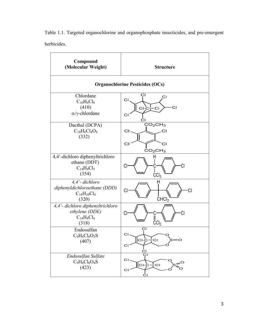
Table 1.1. Targeted organochlorine and organophosphate insecticides, and pre-emergent

herbicide...............................................................................................................................3

Table 1.2. Physical properties for selected pesticides........................................................14

Table 2.1. Hexachlorocyclohexane (HCH) atmospheric concentrations in Canada..........33

Table 2.2. HCH atmospheric concentrations in France.....................................................35

Table 2.3. Atmospheric concentrations of trifluralin in Canada........................................43

Table 2.4. Atmospheric concentration of trifluralin at locations outside of Canada.........45

Table 2.5. Atmospheric concentrations of triallate and ethalfluralin.................................47

Table 4.1. Atmospheric concentrations of -endosulfan and -endosulfan at Bratt’s Lake,

SK during 2007-2010.........................................................................................................66

Table 4.2. Atmospheric concentrations of -HCH and -HCH at Bratt’s Lake, SK during

2007-2010..........................................................................................................................70

Table 4.3. Atmospheric concentrations of triallate and chlorpyrifos at Bratt’s Lake, SK

during 2007-2010...............................................................................................................73

Table 4.4. Atmospheric concentrations of ethalfluralin and trifluralin at Bratt’s Lake, SK

during 2007-2010...............................................................................................................74

Table 4.5. Maximum concentration of pre-emergent herbicides during September and

October-November at Bratt’s Lake, SK.............................................................................85

vii

LIST OF FIGURES

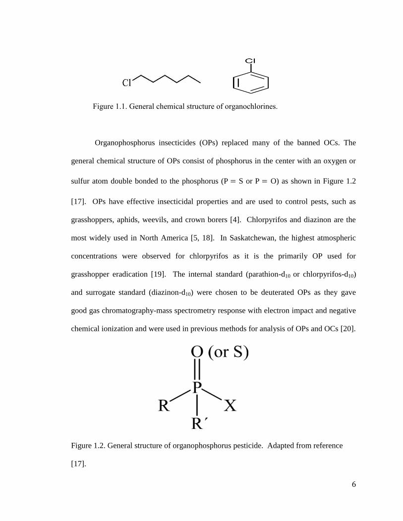
Figure 1.1. General chemical structure of organochlorines.................................................6

Figure 1.2. General structure of organophosphorus pesticide.............................................6

Figure 1.3. Potential behaviours of pesticides in the environment....................................12

Figure 2.1. Usage of selected pesticides in Saskatchewan during 2001-2003. A, Lindane;

B, pre-emergent herbicides................................................................................................50

Figure 3.1. Soil zones in Saskatchewan.............................................................................54

Figure 3.2. High volume air sampler.................................................................................56

Figure 3.3. PUF/Sorbent sampling module........................................................................57

Figure 3.4. Schematic diagram of high-volume air sampler with calibration orifice........58

Figure 4.1. Atmospheric concentrations of and -endosulfan at Bratt’s Lake, SK during

2007-2010..........................................................................................................................69

Figure 4.2. Atmospheric concentrations of -HCH and -HCH at Bratt’s Lake, SK during

2007-2010..........................................................................................................................71

Figure 4.3. Atmospheric concentrations of chlorpyrifos at Bratt’s Lake, SK during 2007-

2010....................................................................................................................................78

Figure 4.4. Atmospheric concentrations of triallate at Bratt’s Lake, SK during 2007-

2010....................................................................................................................................82

Figure 4.5. Total precipitation and daily maximum and minimum temperature at Bratt’s

Lake, SK (2003-2012).......................................................................................................86

Figure 4.6. Atmospheric concentrations of trifluralin at Bratt’s Lake, SK during 2007-

2010....................................................................................................................................88

viii

Figure 4.7. Acres of canola, wheat, durum, and barley harvested in crop districts nearby

to Bratt’s Lake, SK............................................................................................................90

Figure 4.8. Acres of flaxseed, oats, lentils, and peas harvested in crop districts nearby to

Bratt’s Lake, SK.................................................................................................................91

Figure 4.9. Atmospheric concentrations of ethalfluralin at Bratt’s Lake, SK during 2007-

2010....................................................................................................................................93

ix

LIST OF SCHEMES

Scheme 1.1. Oxidative desulfuration of malathion to malathion oxon................................9

Scheme 1.2. EI reaction scheme........................................................................................20

Scheme 1.3. Positive CI reaction scheme..........................................................................20

Scheme 1.4. Processes of negative chemical ionization....................................................22

x

ABBREVIATIONS

2,4-D- 2,4-dichlorophenoxyacetic acid

Ach- acetylcholine

AChE- acetylcholinesterase (enzyme)

BF- bioaccumulation factor

CI- chemical ionization

DCPA - dacthal

DDD - 4,4’-dichlorodiphenyldichloroethane

DDE - 4,4’-dichlorodiphenyldichloroethylene

DDT - 4,4’-dichlorodiphentyltrichloroethane

ECD - electron capture detector

EI - electron ionization

GAPS- global atmospheric passive sampling

GC - gas chromatography

GFF - glass fibre filter

HCH - hexachlorocyclohexane

LC - liquid chromatography

LOD - limit of detection

LRT- long-range transport

MCPA- 2-methyl-4-chlorophenoxyacetic acid

MDL - method detection limit

MS - mass spectrometry

MS/MS - tandem mass spectrometry

xi

NCI - negative ionization

NPD - nitrogen phosphorus detector

OC - organochlorine

OP - organophosphorus

PCI - positive ionization

POP - persistent organic pollutant

PMRA - pesticides management regulatory agency

PSE - pressurized solvent extraction

PUF - polyurethane foam

RT - retention time

SCE- sister-chromatid exchange

SIM - selected ion monitoring

SRM - selected reaction monitoring

UHP - ultra high purity

1

1. INTRODUCTION

This chapter introduces the pesticides and selected organochlorine degradation

products investigated in this thesis. The health impacts of these pesticides, their chemical

properties, and their fate in the environment are discussed. The research objectives in

this project are also described in this chapter.

1.1 Introduction to pesticides

Pesticides are chemicals compounds that are used to control pests, remove

undesirable plants, and enhance agricultural production [1]. There were over 7000

pesticide products registered for use in Canada in 1988 with over 500 active ingredients

[1, 2]. Pesticides can enter the atmosphere through spray drift, post-application

volatilization, and wind erosion of treated soil [1]. This research project investigated

selected pesticides including legacy and current-use organochlorine insecticides (OCs),

pre-emergent herbicides, and an organophosphorus (OP) insecticide.

Organochlorine insecticides (OCs) are a large class of multipurpose chlorinated

hydrocarbons that persist in the environment [3]. OCs and selected OC degradation

products studied in this research project are listed in Table 1.1. OCs contain chlorine-

substituted aliphatic or aromatic rings as shown in Figure 1.1. OCs have insecticidal

properties and have been used to control a wide range of insects such as leafhoppers,

aphids, and corn earworm [4]. 4,4’-Dichloro diphenyltrichloro ethane (DDT) has also

been widely used in Asia to kill malaria and yellow fever-carrying mosquitoes [5, 6].

Some organochlorine pesticides (aldrin, hexachlorocyclohexane (-HCH, -HCH),

lindane (-HCH), chlordane, chlordecone, DDT, dieldrin, endosulfan, endrin, heptachlor,

2

mirex, and toxaphene) are classified as persistent organic pollutants (POPs) due to their

high toxicity, stability, bioaccumulation and long-range transport (LRT) potential [3, 7].

Of these endosulfan is the only pesticide currently registered for use in Canada [8].

Many of the legacy pesticides, which are classified as POPs under the Stockholm

convention, are organochlorines (chlordane, endrin, heptachlor, DDT, lindane (-HCH),

polychlorinated biphenyls (PCBs), -HCH, -HCH) [9]. OC insecticides were widely

used in agriculture and industry in North America [2, 8]. DDT, chlordane, and HCHs

have been banned or restricted globally [10-13]. More recently endosulfan has been

classified as a POP with evidence of its persistent and transport in the environment [9].

Endosulfan is expected to be phased out starting in 2012 worldwide, with its recent

addition to the Stockholm convention on persistent organic pollutants (April 2011) [9].

Some of the currently registered endosulfan products have registration dates beyond 2012

(up to 12/31/2016) [8], but most retail sales are anticipated to end in 2012. Some OCs

such as DDT, were banned due to the toxicity and persistence of their degradation

products. DDT is easily degraded into dichlorodiphenyldichloroethane (DDD) and

dichlorodiphenyldichloroethylene (DDE). These degradation products are more

persistent than DDT. The soil half-life for DDT estimates range from 2-15.6 years [14],

and the soil half-life for DDE is greater than 20 years [15]. DDE causes the inhibition of

prostaglandin which is synthesized in eggshell gland mucosa (particularly p,p-DDE

isomer) leading to eggshell thinning and declining bird populations [16]. Endosulfan

sulfate is a degradation product of endosulfan formed by oxidation [3]. Other degradation

products of OCs that are included in this thesis research include heptachlor and its

subsequent degradation product heptachlor epoxide.

3

Table 1.1. Targeted organochlorine and organophosphate insecticides, and pre-emergent

herbicides.

Compound

(Molecular Weight)

Structure

Organochlorine Pesticides (OCs)

Chlordane

C10H6Cl8

(410)

-chlordane

Dacthal (DCPA)

C10H6Cl4O4

(332)

4,4’-dichloro diphenyltrichloro

ethane (DDT)

C14H9Cl5

(354)

4,4’- dichloro

diphenyldichloroethane (DDD)

C14H10Cl4

(320) 4,4’- dichloro diphenyltrichloro

ethylene (DDE)

C14H8Cl4

(318) Endosulfan

C9H6Cl6O3S

(407)

Endosulfan Sulfate

C9H6Cl6O4S

(423)

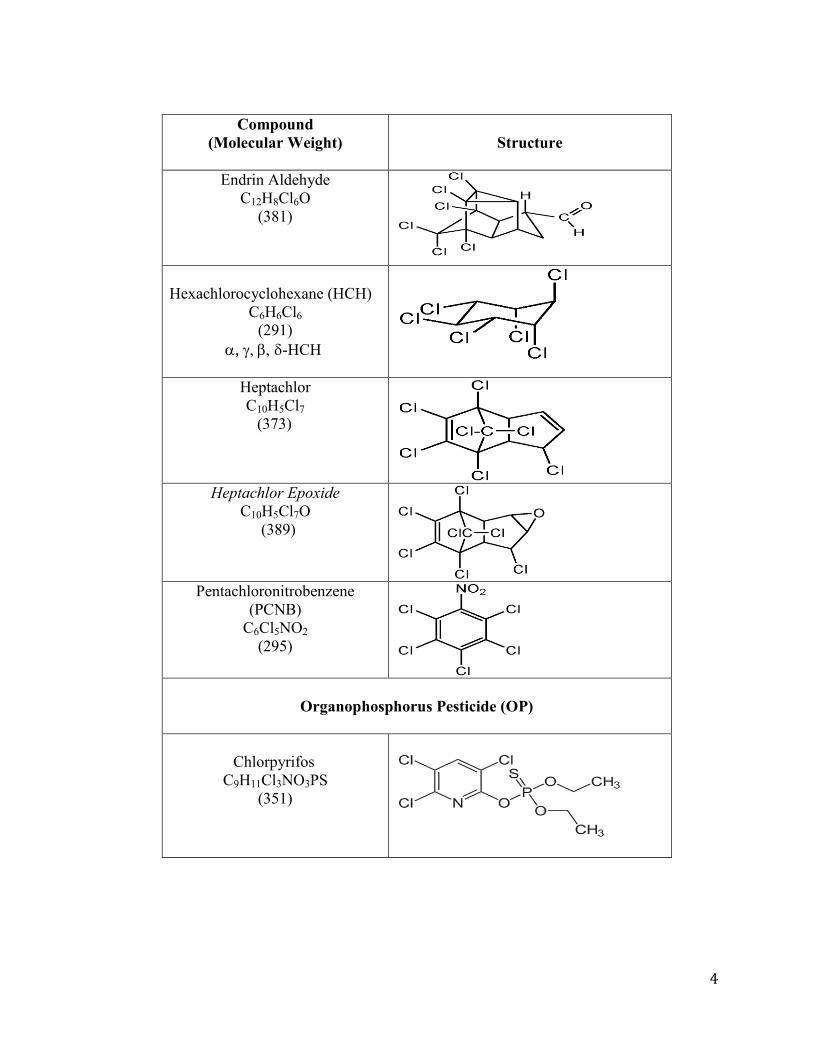
4

Compound

(Molecular Weight)

Structure

Endrin Aldehyde

C12H8Cl6O

(381)

Hexachlorocyclohexane (HCH)

C6H6Cl6

(291)

, , -HCH

Heptachlor

C10H5Cl7

(373)

Heptachlor Epoxide

C10H5Cl7O

(389)

Pentachloronitrobenzene

(PCNB)

C6Cl5NO2

(295)

Organophosphorus Pesticide (OP)

Chlorpyrifos

C9H11Cl3NO3PS

(351)

5

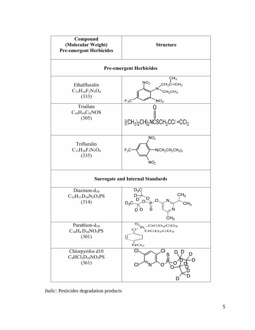
Compound

(Molecular Weight)

Pre-emergent Herbicides

Structure

Pre-emergent Herbicides

Ethalfluralin

C13H14F3N3O4

(333)

Triallate

C10H16Cl3NOS

(305)

Trifluralin

C13H16F3N3O4

(335)

Surrogate and Internal Standards

Diazinon-d10

C12H11D10N2O3PS

(314)

Parathion-d10

C10H4 D10NO5PS

(301)

Chlorpyrifos d10

C9HCl3D10NO3PS

(361)

Italic: Pesticides degradation products

6

Figure 1.1. General chemical structure of organochlorines.

Organophosphorus insecticides (OPs) replaced many of the banned OCs. The

general chemical structure of OPs consist of phosphorus in the center with an oxygen or

sulfur atom double bonded to the phosphorus (P S or P O) as shown in Figure 1.2

[17]. OPs have effective insecticidal properties and are used to control pests, such as

grasshoppers, aphids, weevils, and crown borers [4]. Chlorpyrifos and diazinon are the

most widely used in North America [5, 18]. In Saskatchewan, the highest atmospheric

concentrations were observed for chlorpyrifos as it is the primarily OP used for

grasshopper eradication [19]. The internal standard (parathion-d10 or chlorpyrifos-d10)

and surrogate standard (diazinon-d10) were chosen to be deuterated OPs as they gave

good gas chromatography-mass spectrometry response with electron impact and negative

chemical ionization and were used in previous methods for analysis of OPs and OCs [20].

Figure 1.2. General structure of organophosphorus pesticide. Adapted from reference

[17].

7

Triallate, trifluralin, and ethalfluralin are pre-emergent herbicides which are

widely used on crops such as wheat, barley, canola, flaxseed, lentils, and peas in the

prairies (provinces of Alberta, Saskatchewan, Manitoba) [4, 6]. Ethalfluralin is also used

on sunflower seeds, dry beans, peanuts, and soybeans [4]. Triallate is primarily used for

weed control for wheat and barley, while trifluralin has been more commonly used for

weed control for wheat and canola in the Canadian prairies as well as other crops more

commonly grown in the United States such as soybeans and cotton [4]. Triallate is not

recommended for use for weed control for canola. Triallate is a thiocarbamate herbicide,

and trifluralin and ethalfluralin are dinitroaniline herbicides.

1.2 Health and environmental impacts of target pesticides

Pesticides of greatest concern are those that exhibit persistence, high toxicity,

bioaccumulation, and long- range transport potential [3]. OCs can bioaccumulate in the

food chain and are found in fatty tissues of mammals as well as humans [7, 21]. OCs

have been detected in water, soil, animals, and traditional food supplies such as meat,

dairy and fish [22]. As OCs bioaccumulate in the food chain, their presence in fatty

tissues is of concern for human health due to the exposure to these pesticides in

traditional diets. Exposure to OCs (DDT, DDE, PCBs, HCHs, endosulfan, and

chlordane) can lead to adverse health effects such as cancer and neurodegenerative

diseases [23]. Bioaccumulation of pesticides is defined by the bioaccumulation factor

(BF), where BF for OCs is > 5x103 [3]. A study of women from an agriculture area in

India reported levels of DDT and DDE above 10 g/L in mother’s blood [24]. Higher

incidences of breast cancer in women have been associated with high concentrations of

8

DDT in their blood [24]. Fetuses and children can be exposed to pesticides in utero and

through breast milk. In Zimbabwe, the national average concentration of DDT in breast

milk was high ( 6,000 ng/g DDT in lipid) [8, 25]. DDE causes premature birth and has

been reported at concentrations greater than 0.61 g/L in mother’s serum [26]. Northern

aboriginal people depend on high-fat country foods in their diet and as a result of

bioaccumulation in the food chain these fatty foods tend to contain high concentrations of

OC contaminants [27]. OCs have also been found a variety of mammals worldwide. For

example, dolphin’s feed on a variety of fish and as a consequence of this diet,

concentrations of DDT and PCB in fat tissues have been reported as high as 103 and 150

g/g, respectively [3, 21]. In polar bear fat tissues collected during the period of 1978-

1989 observed concentrations of DDE ranging from less than 0.10 to 3.40 g/g [28]. The

total HCH concentration in polar bears was 0.07 – 0.59 g/g lipid for samples collected

during the period of 1996-2002 [29]. The highest HCH concentrations were found in

Alaskan samples and the lowest concentrations in Svalbard samples [29]. Concentrations

of HCH and DDT in fatty tissues of ringed seals were 0.004 and 0.220 g/g, respectively

[30]. Endosulfan concentrations are generally lower than DDT in samples but above

detectable limits. Endosulfan was reported in the fat and blood of polar bear samples

from the southern Beaufort Sea. The average concentrations of both α and β-endosulfan

were 0.004 g/g lipid [31]. A study during 1991-2002 on concentrations of chlorinated

compounds in plasma samples of Canadian’s living in Quebec of age group 18-74 years

showed PCBs at 0.153 g/g lipid [32].

OPs are neurotoxins and can target the central nervous system in humans by

inhibiting the enzyme acetylcholinesterase (AChE) [33]. AChE is responsible for the

9

transmission of nerve impulses. The OPs interfere with the metabolism of acetylcholine

(ACh) causing the inhibiting of AChE [33]. The body accumulates ACh and this can

lead to headaches, anxiety, confusion, convulsions, and ataxia [33]. Humans can be

exposed to OPs by inhalation, ingestion, and dermal absorption [33]. Symptoms of acute

exposure to OPs were examined in farm workers after acute exposure to various OPs,

such as chlorpyrifos. These workers report anxiety, depression, irritability, confusion, and

impaired concentration and memory [33]. In addition to impacts of OPs on the central

nervous system, long-term exposure to OPs has been associated with increased

incidences of cancer and asthma [33, 34]. Exposure to OPs such as chlorpyrifos has been

linked to increased incidences of brain cancer where brain cancer was found in 142 out of

389 orchard-farm workers who were exposed to OPs at an early age of 10- 20 years [35].

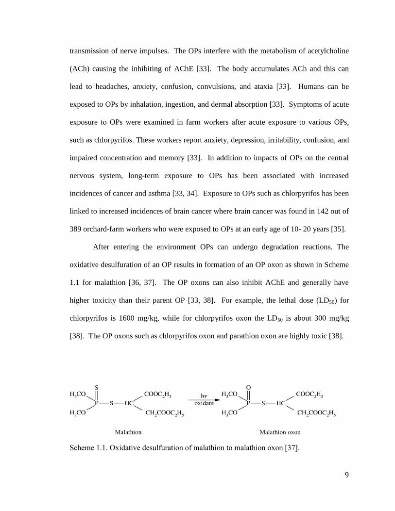
After entering the environment OPs can undergo degradation reactions. The

oxidative desulfuration of an OP results in formation of an OP oxon as shown in Scheme

1.1 for malathion [36, 37]. The OP oxons can also inhibit AChE and generally have

higher toxicity than their parent OP [33, 38]. For example, the lethal dose (LD50) for

chlorpyrifos is 1600 mg/kg, while for chlorpyrifos oxon the LD50 is about 300 mg/kg

[38]. The OP oxons such as chlorpyrifos oxon and parathion oxon are highly toxic [38].

Scheme 1.1. Oxidative desulfuration of malathion to malathion oxon [37].

10

Exposure of humans to pre-emergent herbicides has been associated with a variety

of health effects including impaired development, non-Hodgkin’s lymphoma, and

prostate cancer [39, 40]. The genotoxicity of pre-emergent herbicides such as trifluralin

has been evaluated by using human peripheral blood lymphocytes samples [40].

Trifluralin is able to exert a weak cytotoxic effect in cultured human lymphocytes [40].

Increase in sister-chromatid exchange (SCE) levels leads to a reduction of cell

proliferation when concentrations of SCE ranged from 0-200 g/mL [40]. Another study

of the genotoxicity of trifluralin in human peripheral blood lymphocytes samples showed

a significant increase in the tail length of the DNA which is considered to be DNA

damage [41]. The concentrations of trifluralin were 25, 50, and 100 g/mL for these

exposure studies. Pre-emergent herbicides were analyzed in plasma samples collected

from rural residents of a cereal producing region of Saskatchewan during the spring

herbicide application period of June–July 1996. Concentrations of triallate, trifluralin,

and ethalfluralin were observed in the plasma ranged 1-20, 1-13, and 1-13 μg/L,

respectively) and indicates there is potential for the pre-emergent herbicides at these

concentrations to result in DNA damage [42]. DNA damage in human has also been

associated with exposure to OPs [34].

11

1.3 Pesticides in the environment

Pesticides after application are released into the environment where they can be

transported through the environment, or transformed. Pesticides have been detected in

the four main compartments of the environment: air, water, soil and living organisms.

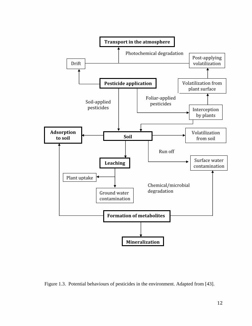
Figure 1.3 summarizes the processes pesticides can undergo after they enter the

environment [43]. Pesticides can be applied as a spray or in a granular form to a field.

Pesticides move from the targeted agricultural area through spray drift, volatilization, or

runoff. After application, pesticides that enter the atmosphere can travel in the gas or

particle phase far from their original application site. Pesticides will settle out of the

atmosphere by a dry deposition processes or precipitation. After deposition, pesticides

can re-enter the atmosphere by re-volatilization from soil, vegetation, or water surfaces.

For pesticides such as OCs, atmospheric transport is the main pathway of movement from

regions where they were initially applied to other areas such as the Arctic. For pesticides

with higher water solubility, transport in water may be significant.

12

Figure 1.3. Potential behaviours of pesticides in the environment. Adapted from [43].

Transport in the atmosphere

Soil contamination

Mineralization

Formation of metabolites

Volatilization from soil surface

Surface water contamination

Leaching

Ground water contamination

Plant uptake

Pesticide application

Interception by plants

Volatilization from plant surface

Post-applying volatilization Drift

Photochemical degradation

Adsorption to soil matrix

Soil-applied pesticides

Foliar-applied pesticides

Run off

Chemical/microbial degradation

13

1.4 Chemical properties of target pesticides

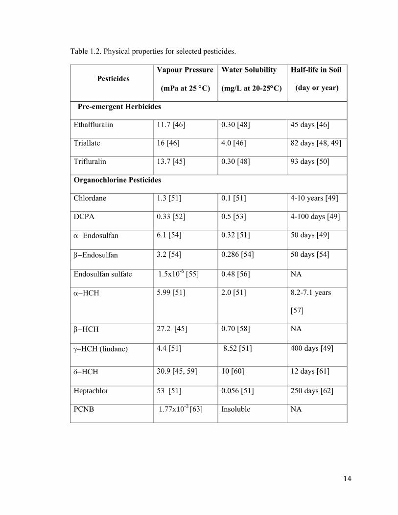
Pesticides have different chemical and physical properties. Water solubility,

vapour pressure, and half-life may vary from one pesticide to another [2]. Table 1.2

shows the range in water solubility, vapour pressure, and half-life in soil for a number of

the pesticides included in my thesis. Pathways of movement of OCs in the environment

include atmospheric transport, water transport such as by major ocean currents, and

animal migration along with subsequent bioaccumulation in the food chain [44].

Pesticides with higher vapour pressure and low water solubility will undergo atmospheric

transport more readily than other transport pathways. The pre-emergent herbicides are

examples of pesticides that more readily undergo atmospheric transport than transport

through water bodies. Table 1.2 shows that the pre-emergent herbicides such as triallate,

trifluralin, and ethalfluralin have high vapour pressures and low water solubility [45, 46].

In comparison, the phenoxyacid herbicides have high water solubility and relatively low

vapour pressure such that water transport is a more important pathway of movement in

the environment. Chlorpyrifos has relatively high vapour pressure and has been detected

at high concentrations in the atmosphere [19]. OCs are considered volatile with vapour

pressures that range from 1.3-53 mPa at 25 C for -HCH,-HCH (lindane), -

endosulfan and -endosulfan (see Table 1.2).

Generally, pesticides with vapour pressures higher than 101 mPa are observed

predominately in the gas phase, while pesticides with lower vapour pressure than 10-2

mPa can partition into the particle phase. The pre-emergent herbicides and chlorpyrifos

are found predominately in the gas phase in the atmosphere [7, 47]

14

Table 1.2. Physical properties for selected pesticides.

Pesticides

Vapour Pressure

(mPa at 25 C)

Water Solubility

(mg/L at 20-25C)

Half-life in Soil

(day or year)

Pre-emergent Herbicides

Ethalfluralin 11.7 [46] 0.30 [48] 45 days [46]

Triallate 16 [46] 4.0 [46] 82 days [48, 49]

Trifluralin 13.7 [45] 0.30 [48] 93 days [50]

Organochlorine Pesticides

Chlordane 1.3 [51] 0.1 [51] 4-10 years [49]

DCPA 0.33 [52] 0.5 [53] 4-100 days [49]

Endosulfan 6.1 [54] 0.32 [51] 50 days [49]

Endosulfan 3.2 [54] 0.286 [54] 50 days [54]

Endosulfan sulfate 1.5x10

-6 [55] 0.48 [56] NA

HCH 5.99 [51] 2.0 [51] 8.2-7.1 years

[57]

HCH 27.2 [45] 0.70 [58] NA

HCH (lindane) 4.4 [51] 8.52 [51] 400 days [49]

HCH 30.9 [45, 59] 10 [60] 12 days [61]

Heptachlor 53 [51] 0.056 [51] 250 days [62]

PCNB 1.77x10-3

[63] Insoluble NA

15

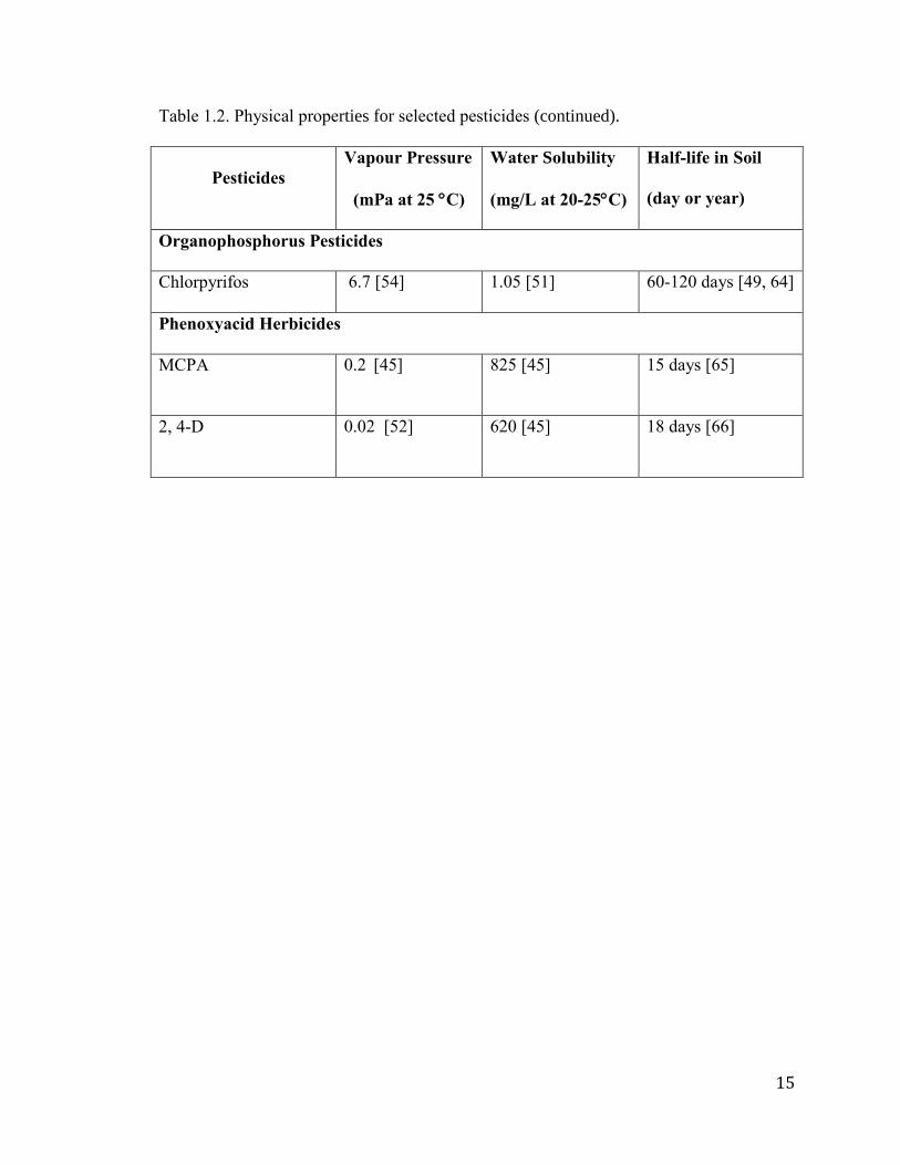
Table 1.2. Physical properties for selected pesticides (continued).

Pesticides

Vapour Pressure

(mPa at 25 C)

Water Solubility

(mg/L at 20-25C)

Half-life in Soil

(day or year)

Organophosphorus Pesticides

Chlorpyrifos 6.7 [54] 1.05 [51] 60-120 days [49, 64]

Phenoxyacid Herbicides

MCPA 0.2 [45]

825 [45] 15 days [65]

2, 4-D 0.02 [52]

620 [45] 18 days [66]

16

In general pesticides that have vapour pressures lower than 10-4

mPa at 20 C are less

likely to undergo volatilization directly into the gas phase [67]. Pesticides with lower

vapour pressure can still be transported in the atmosphere in the particle phase [68].

Concentrations of pesticides in the atmosphere (in gas or particle phase) are also

influenced by usage of pesticides particularly locally or regionally.

Atmospheric transport has been identified as a major pathway of movement of

OCs from regions where they were initially applied to other areas such as the Arctic.

OCs are predominately observed in the gas phase with higher concentrations generally

observed in the summer as expected from increased volatilization with higher

temperatures. Higher concentrations of -HCH in the gas phase have been observed in

the summer in the Arctic [27], and the vapour pressure of -HCH is 30.9 mPa at 20-25 C

[45, 59]. Endosulfan ( or isomer) is the most commonly observed organochlorine in

the atmosphere throughout North America and the Arctic and prior to 2013 was still used

in many countries [1, 7, 69].

Water solubility is another property that provides information of the movement of

pesticides into the water phase. The water transport pathway is also a significant pathway

of movement of OCs in the environment [27]. Pesticides can move into the water phase

either directly from soil or vegetation surfaces (such as from runoff) or from wet

deposition. Water solubility of OCs ranges from 0.05-10 mg/L at 20-25 C (see Table

1.2). OCs water solubility are relatively low in comparison to phenoxyacid herbicides

such as 2-methyl-4-chlorophenoxyacetic acid (MCPA) and 2,4-dichlorophenoxyacetic

acid (2,4-D) which have water solubility’s of 825 mg/L, and 620 mg/L, respectively [34].

MCPA and 2,4-D are more likely to undergo water transport than atmospheric transport

17

[70]. However, OCs such as endosulfan still have sufficient water solubility that enables

their movement in water. Endosulfan has been detected in fresh water and marine water

samples at 0.02 g/L and 0.001 g/L, respectively [69]. Its presence in water is also

associated with current usage of endosulfan in China, India, Europe, United States, and

Canada [69]. The pre-emergent herbicides have high vapour pressure and also have

relatively low water solubility (triallate 4.0 mg/L, see Table 1.2) and found at low levels

in precipitation or surface water [46].

The pesticides investigated also have soil half-life typically greater than 45 days

(see Table 1.2) such that detection of these pesticides in the atmosphere throughout the

agricultural season is expected. Some OCs have very long soil half-lives such that they

persist in soil and thus can volatilize for a long time after application often leading to

year-long detections. Endosulfan and lindane (-HCH) have been detected in the

atmosphere in the Canadian prairies long after their application period [1, 7].

Pesticides undergo degradation and transformations in the atmosphere that will

decrease their atmospheric concentrations [61]. This can be occur through direct

photochemical reactions with sunlight or an indirect reaction with radicals (·OH)

generated during photolysis. Some OCs such as -HCH have a longer half-life in the

atmosphere (12 days) as compared to other pesticides such as trans-chlordane which

undergoes photo-degradation readily in the atmosphere [61]. Trans-chlordane undergoes

photo-degradation to cis-chlordane, and higher levels of cis-chlordane in the atmosphere

are found in summer than in winter [1, 27]. As -HCH is stable in the atmosphere it can

be transported long distances in the atmosphere such that it can be detected in the Arctic

[27, 61]. Previous atmospheric measurements taken when lindane was still registered for

18

use in Canada showed that the Canadian prairies was a primary source region of -HCH

[71, 72]. OPs such as chlorpyrifos undergo degradation in the atmosphere through the

oxidative desulfuration process to form an OP oxon [19]. Chlorpyrifos oxon atmospheric

concentrations and ratio of chlorpyrifos oxon/chlorpryifos in the atmosphere increase in

summer as expected from increasing degradation of chlorpyrifos in the summer with

increasing hours of sunlight and oxidant concentrations [19].

1.5 Analytical method

The pesticides selected for my thesis research were previously detected at Bratt’s

Lake and can be analyzed by gas chromatography (GC) [6, 19, 20, 73]. GC is the most

common method for separating pesticides that have low polarity, high volatility, and

thermal stability. The maximum temperature used in the temperature program for the

separation is limited by the choice of column (stationary phase) which have maximum

temperature limits in the range of 250-300 C [20, 74-76]. The mobile phase for GC is

called the carrier gas and is a chemically inert gas such as helium. For the separation of

relatively non-polar pesticides (such as OCs), a nonpolar stationary phase such as 5%

diphenyl/95% dimethylpoysiloxane should be chosen [20]. After the separation of the

analyte by GC, a detection step is required for analyte quantitation. Different detectors

including electron capture detector (ECD), nitrogen-phosphorus detector (NPD), and

mass spectrometry (MS) have been used [20, 77-79]. When non-selective detectors such

as ECD or NDP are used, the identification of the analyte is based on retention time (RT)

match and generally confirmation of identity of the analyte is accomplished by

19

performing the separation of the analytes on two different polarity stationary phases or

using different detectors [20, 71, 80].

GC/MS is the most common method for pesticides analysis due to its added

confirmation ability [81]. It is a selective detector which can provide information about

the molecular weight or structure of the analyte. After the set-up of the method (using

scans for pesticide confirmation) the quantitation and confirmation is performed by

monitoring the abundance at two or more mass-to-charge ratios (m/z) along with

confirmation by retention time (RT) match [20, 76, 80, 82, 83]. The peak areas measured

for the most intense ion are used for quantitation, while ratio of response (as peak area) of

the two ions and RT are used for confirmation [20]. This ratio and its % relative standard

deviation is determined from standards run on the day of analysis and this ratio must be

obtained for the sample within a specified % relative standard deviation for confirmation

of identity of the target pesticide [20].

The ionization of pesticides in GC/MS can be done in two different ways:

electron ionization (EI) or chemical ionization (CI) [20, 80, 82-86]. EI involves a heated

filament giving off electrons that are accelerated and collide with the gaseous sample

molecules. This collision causes ionization through the loss of an electron resulting in

the formation of a positive molecular ion (M+

) or fragment ions (A+, B

+) or neutral loss

(C) as shown in (Scheme 1.2, reaction 1 and 2). The positive ions are directed through

ion optics into the mass analyzer. The ion optics consist of a series of lenses which focus

the ions into the mass analyzer where they are separated based on mass-to-charge ratio

(m/z).

20

e + M M

+ + 2 e

(1)

or

e + M M

+ + 2 e

+ A

+ + B

+ + C (2)

Scheme 1.2. EI reaction scheme. M is the sample molecule; M+

is the positive

molecular ion; A+ , B

+ are smaller mass positive ions; and C is a neutral fragment. Taken

from [86].

In chemical ionization (CI), electrons are produced by a filament in the ion source

as in electron impact ionization, but a reagent gas is also present in the ion source.

Because the number of reagent gas molecules is greater than the sample molecules, the

gas molecules are ionized with greater efficiency as shown in Scheme 1.3, reaction 1. In

positive chemical ionization (PCI) the initial reagent gas radical ion (G+·

) further reacts

with other reagent gas molecules (Scheme 1.3, reaction 2) producing the reactive gas ion

(G+H)+. The reactive gas ion (G+H)

+ then reacts with the sample molecules to produce

the protonated molecular ion (M+H) +

[86].

G + e G

+. + 2 e

(1)

G + G+.

(G+H)+ + (G-H)

. (2)

(G+H)+ + M G + (M+H)

+ (3)

Scheme 1.3. Positive CI reaction scheme. G is the reagent gas; G+ is the initial reagent

gas ion; (G+H)+ is the reactive gas ion; and (M+H)

+ is the protonated molecular ion.

Taken from [86].

21

CI can be performed in positive (PCI) or negative (NCI) modes. In PCI the

ionization occurs when the analyte molecule reacts with the reactive gas ion (G+H)+.

This approach is generally not used for environmental analysis as it suffers from high

background signal due to interfering matrix components that are also ionized [20, 87, 88].

In NCI the reagent gas role is to slow the electrons such that the fragmentation is

generally a softer process than in EI or PCI. Analyte molecules react with these lower

energy electrons in the reagent gas to produce a negative molecular or fragment ion as

shown in Scheme 1.4 [86]. Electrons can be captured by three different mechanism to

produce the negative ion (Scheme 1.4). For a negative ion to be produced the sample

molecule must be capable of capturing electrons. Pesticides are good candidates for NCI

as many are halogenated and thus capable of capturing electrons. Pesticides analyzed by

GC generally fragment in the ion source even with negative chemical ionization and MS

spectra often have low abundance of the negative molecular ion (M-

) [20, 81]. NCI is

more selective than PCI as many of the interfering matrix compounds are hydrocarbons

in environmental samples which do not ionize and consequently NCI is more frequently

used for analysis of pesticides in environment samples [20, 84-86, 89, 90]. A comparison

of different ionization techniques for the GC/MS analysis of pesticides including those

analyzed in this thesis research showed that NCI provided the lowest detection and added

selectivity for air extracts [20]. NCI is more sensitive by at least one order of magnitude

as compared to EI with GC/MS for many organochlorines [20, 84].

AB + e AB

(associative resonance capture)

22

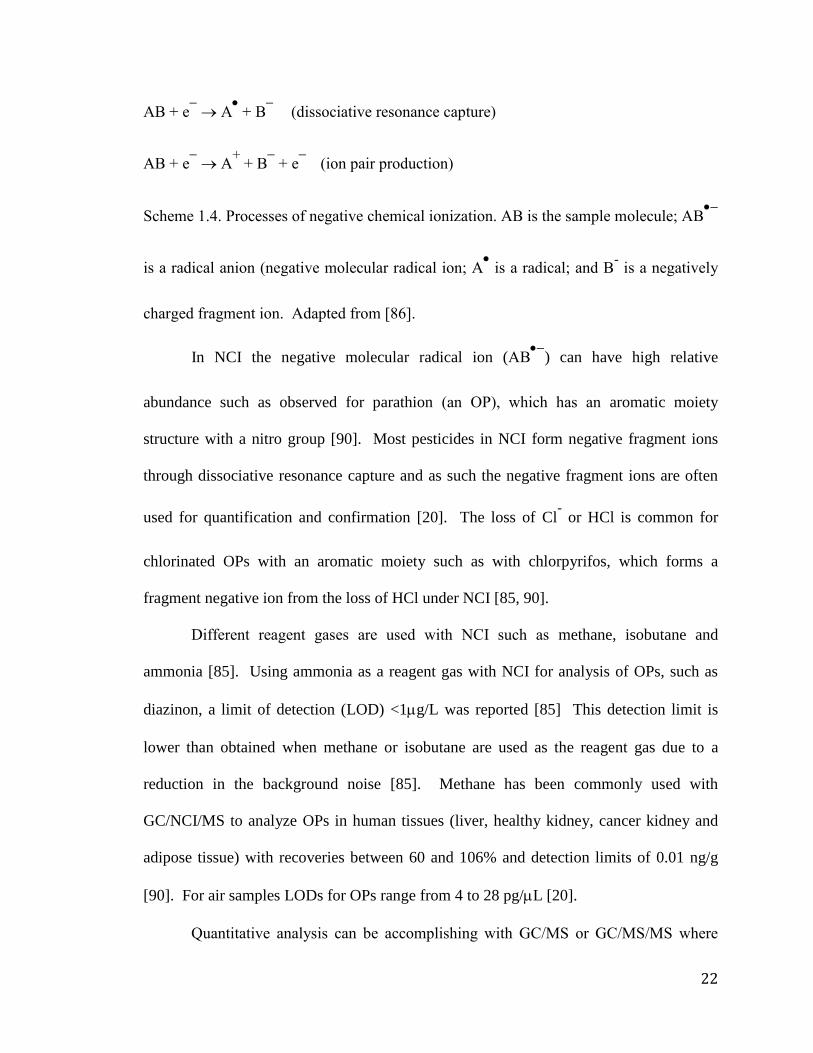
AB + e A

+ B

(dissociative resonance capture)

AB + e A

+ + B

+ e

(ion pair production)

Scheme 1.4. Processes of negative chemical ionization. AB is the sample molecule; AB

is a radical anion (negative molecular radical ion; A

is a radical; and B- is a negatively

charged fragment ion. Adapted from [86].

In NCI the negative molecular radical ion (AB

) can have high relative

abundance such as observed for parathion (an OP), which has an aromatic moiety

structure with a nitro group [90]. Most pesticides in NCI form negative fragment ions

through dissociative resonance capture and as such the negative fragment ions are often

used for quantification and confirmation [20]. The loss of Cl- or HCl is common for

chlorinated OPs with an aromatic moiety such as with chlorpyrifos, which forms a

fragment negative ion from the loss of HCl under NCI [85, 90].

Different reagent gases are used with NCI such as methane, isobutane and

ammonia [85]. Using ammonia as a reagent gas with NCI for analysis of OPs, such as

diazinon, a limit of detection (LOD) <1g/L was reported [85] This detection limit is

lower than obtained when methane or isobutane are used as the reagent gas due to a

reduction in the background noise [85]. Methane has been commonly used with

GC/NCI/MS to analyze OPs in human tissues (liver, healthy kidney, cancer kidney and

adipose tissue) with recoveries between 60 and 106% and detection limits of 0.01 ng/g

[90]. For air samples LODs for OPs range from 4 to 28 pg/L [20].

Quantitative analysis can be accomplishing with GC/MS or GC/MS/MS where

23

one or two stages of mass selection are used. In GC/MS selected ion monitoring (SIM)

mode is used, while for GC/MS/MS selected reaction monitoring (SRM) is used [20]. In

SIM mode typically two ions are monitored in the mass analyzer for each analyte. The

highest abundance ion is monitored for quantification and the second most abundant ion

is monitored for confirmation. For example, for EI-SIM two ions are monitored for each

pesticides (chlorpyrifos (197/314) and diazinon (179/137)) with the underlined masses

(m/z) used for quantification (target ions), while the other masses (m/z) are used for the

confirmation of a specific pesticide (qualifier ions) [80]. In NCI-SIM the higher mass

ions for OCs or OPs can contain chlorine with chlorine isotope clusters observed [84].

For example, endosulfan ( and ) has a high abundant ion cluster at m/z 404 (and

corresponding isotope peaks) due to the molecular ion along with a high fragment mass

ion at m/z of 372 (and its corresponding isotope peaks). The most abundant ions for

endosulfan ( and ) are at m/z 372, 404, and 406 [20, 80].

In tandem MS (MS/MS) an ion is selected in the first quadrupole, then undergoes

fragmentation in the collision cell which is a quadrupole or hexapole. The fragment ion

is selected and detected in the third quadrupole which acts as the second mass analysis

stage [86]. A SRM transition represents the mass/charge ratio for this fragmentation

process where m1- > f1

- (selected negative ion > fragment negative ion) such as the SRM

transition of 406 >35 for -endosulfan where the selected ion is an isotope peak of the

molecular ion M-

(MW=404) and m/z of 35 corresponds to the fragment ion Cl- [20].

The advantages of using this technique over MS is that it can be more selective as

background noise and interferences are reduced [20, 91]. Reduced analysis time may

also occur if interferences do not need to be separated from analyte components [76, 91].

24

1.6 Research objectives

The present study examines selected organochlorine insecticides, an

organophosphorus insecticide (chlorpyrifos), and pre-emergent herbicides in the prairie

agricultural region. Previous studies showed strong evidence for the occurrence of some

of these pesticides in the atmosphere and in some cases distinctive seasonal variations.

My research project is a continuation of these earlier studies to provide long-term trends

in the variation of atmospheric concentrations of these pesticides that were previously

detected.

The main objectives of the present study can be summarized as follows:

To determine changes in atmospheric concentrations of selected pesticides over

several years to assess shifts in atmospheric concentrations on a seasonal or

annual basis. To use the changes in atmospheric concentrations of individual

pesticides to assess where there may be shifts in usage of pesticides (usage data

only available for 2003 for Saskatchewan).

To provide insight into the relationship of atmospheric concentrations of these

pesticides with changes in climate or agricultural factors such as changes in

precipitation, temperature, crop land or production rates.

To provide insight into changes in the relative importance of local, regional, and

long-range atmospheric transport with these variations in atmospheric

concentrations.

25

2. LITERATURE REVIEW

2.1 Analysis methods of pesticide

GC/NCI/MS has been used for the analysis of OC pesticides in a wide variety of

sample matrices [20, 84, 85, 89, 90]. HCH, endrin, heptachlor, and -endosulfan were

detected in plasma samples from wild birds with a LOD of 0.036-0.307 pg/L [84].

DDT, DDE, DDD, endrin and heptachlor were detected selectively using GC/MS with

NCI [89]. This study reported improvements with NCI due to reduction in background

signal with no interfering peaks observed and LOD less than 5 pg/L [89]. LOD of 0.15-

88.82 pg/ml for these pesticides was reported in fruits and vegetable samples [84]. In

human tissues samples LOD for OCs was in the range of 0.01-0.09 ng/g [90]. LOD was

lower (<1 pg/L) in complex matrices (plant, animals) [85].

NCI is also valuable as a reference technique for analysis of OPs. The

electrophilic molecular structure of OPs allows for electron capture necessary for NCI

[85]. OPs were detected in different types of samples such as food (fruits, vegetables,

meat, fish), water, animal and human tissues using GC/MS with NCI [90]. The LOD was

0.002 pg/L for the analysis of chlorpyrifos and diazinon in human tissues samples when

NCI was [85, 90]. The analysis of OPs including chlorpyrifos and diazinon in air extracts

was also accomplished by GC/MS with NCI with LOD of 5.1 and 3.9 pg/L, respectively

[20].

For quantitative analysis the quantitative ion (or SRM transition) is selected as the

most abundant ion (or SRM transition), while the qualifier ion is the second most

abundant ion (or SRM transition) with m/z selected above m/z of 70 when possible to

26

reduce the impact of interferences [20, 91]. Chlorpyrifos has m/z of 97, 197, 199, and 29

as the four most abundant ions in its EI spectra, although 314 and 316 are also observed

[20, 90, 91]. For quantitation at trace level the abundances at m/z 97 and 197 were

monitored instead of m/z of 314 and 316, because of their higher abundances [20]. These

ions are also above m/z of 70, which makes them less prone to interferences. The

abundance at 314 and 316 was too low for confirmation analysis [20]. EI-SRM is less

sensitive for a large number of OPs (except for parathion). Sensitivity is particularly low

for chlorpyrifos because the abundance of molecular ion is very low (<10%), minimizing

the potential for collision-induced dissociation in GC/MS/MS [20, 91]. NCI is the best

option for quantitative analysis as it has the lowest detection limits with greater potential

for high mass ions to be selected as the quantitative or qualifier ion as NCI is a softer

ionization process than EI [20, 82, 90]. NCI-SRM can provide higher abundance of

molecular ion than EI-SRM. However, similar to EI and PCI the most abundant ions are

still frequently fragment ions. As a fragment ion frequently needs to be selected for

collision-induced dissociation for SRM, the detection limits for NCI-SRM are often

higher than with NCI-SIM. A number of pesticides can be analyzed by NCI-SRM where

a fragment ion undergoes further fragmentation such that a sensitive SRM transition is

observed. HCH isomers have the SRM transitions of 73>37 or 71>35 where Cl-

(m/z=35

and 37) is produced from the collision induced dissociation of the fragment ion (m/z=71,

73) [20, 90]. NCI-SRM can provide added selectively where an additional confirmation

approach is required. GC-NCI/SIM provides the lowest method detection limits of 2.5-

10 pg/μL for a range of OCs and OPs pesticides [20, 80], and for ethalfluralin, trifluralin,

chlorpyrifos, and lindane at 0.10, 0.13, 0.12, and 0.04 mg/L, respectively [79]. NCI-SIM

27

also has high confirmation ability, with relative standard deviation of the ratios of

response of quantitative/qualifier ion generally <15% [20, 80, 82]. SIM mode has been

commonly used for the analysis of pesticides, and for the pesticides examined in this

thesis NCI-SIM is more sensitive than NCI-SRM, although NCI-SRM can provide added

confirmation [20, 80-82, 84, 91, 92].

2.2 Atmospheric concentrations of pesticides

Endosulfan is the only currently registered OC pesticide in Canada and has been

widely used across Canada [75]. Endosulfan was added to the Stockholm Convention in

2011 with a ban or phase-out of its use from market expected in mid-2012 in most

countries. Some limited use exceptions will continue for an additional 5-11 years in

countries such as India. India is the largest manufacturer and user of endosulfan with

total emissions estimated around 150 kt [93]. Some of the currently registered

endosulfan products in Canada have registration dates beyond 2012 (up to 12/31/2016)

[8], but most retail sales are anticipated to end in 2012. In the United States phase out is

expected by 2016 [94]. Endosulfan is a contact insecticide used on a large variety of

vegetables, fruits and cereal crops [7]. In Saskatchewan it is recommended for used on

bean, corn, potato, alfalfa and sunflower, with beans having the greatest production [4].

Usage in Saskatchewan has been very low with no reported usage in 2003 [5]. The

eastern provinces (NB, NS, and PEI), Ontario, and British Columbia have had the highest

reported usage of endosulfan in 2003 [75].

Endosulfan consists of two isomers, -endosulfan and -endosulfan in a ratio of

7/3 [7]. In 1986, -endosulfan was first detected in snow samples from different

28

locations in the Arctic with an average concentration of 410 pg/L [7]. In 1993, -

endosulfan was detected in more than 90% of the air samples at Alert, at maximum of

94.2 pg/m3, and an average air concentration of 3.6 pg/m

3 [7]. In comparison, during

1996 and1997 maximum concentrations of endosulfan at Agassiz (located in the eastern

end of the Lower Fraser Valley, British Columbia) were 2600 and 550 pg/m3 for and -

endosulfan, respectively [7]. At Abbotsford, BC in the middle of the Lower Fraser

Valley, the peak atmospheric concentrations during 1996-1997 were at 2310 and 650 pg/

m3 for and -endosulfan, respectively [7]. In another study in British Columbia during

2001 the atmospheric air concentrations of endosulfan were found to be higher at an

agricultural site as compared to an urban site. Air concentrations of and -endosulfan

at the rural agricultural site in Langley, BC ranged from ~18-82 pg/m3

compared to an

urban site, Slocan, with concentrations of endosulfan ranging from 4-62 pg/m3

[95].

However, these atmospheric concentrations of endosulfan in BC were considerably lower

than in north of Toronto. In 2000 at the urban-rural passive sampling site at Egbert

atmospheric concentrations of total endosulfan were reported in range 400-800 pg/m3 [7,

95]. The presence of these high atmospheric concentrations of endosulfan were attributed

to its wide use on a variety of vegetables and fruits [7].

In 2005 measurements at the CN Tower in Toronto showed the strongest seasonal

variations in atmospheric concentrations of endosulfan isomers with highest

concentrations observed during the spring at 700 pg/m3 for -endosulfan, and 200

pg/m3 for -endosulfan [96]. This was associated with use of endosulfan on a wide

variety of crops in southern Ontario and other more southern regions of North and South

America. During 2003 the highest air concentration of and -isomers in Canada were

29

observed at Kensington, PEI at approximately 8000 pg/ m3

[1]. This site is in an area of

high potato production. Atmospheric concentrations have declines in 2004 and 2005 at

Kensington to <1000 pg/m3

[2]. At Bratt’s Lake, SK the atmospheric average

concentration of -endosulfan was 1.77 pg/m3 in 2003, while the maximum concentration

was 5.12 pg/m3 [6].

In 2001, endosulfan was reported at four sites in different States in the United

States (Michigan, Indiana, Arkansas, and Louisiana) with the median concentration in the

range 37-79 pg/m3 [95, 97]. The endosulfan air concentrations during the period of June

and July 2002-2003 at the Michigan site were in the range 690-1200 pg/m3 and at a site in

Indiana during July and August were in the range 1020-2000 pg/m3. The air

concentrations of endosulfan at the Michigan and Indiana sites were similar and about 3

times higher than those at Arkansas and Louisiana sites [97]. The high concentrations of

endosulfan at the Michigan and Indiana sites were associated with direct agricultural

application on crops such as cotton, melon, and tomatoes grown around the sites [97, 98].

-endosulfan was detected in lesser amounts than the -isomer generally in the

atmosphere as :-endosulfan ratio is 7:3 in formulations and the -isomer is more

volatile (vapor pressure 6.1 mPa, and 3.2 mPa at 25 C for -endosulfan and -

endosulfan, respectively) [7, 54]. -endosulfan is also less stable and converts to the -

isomer in the environment after application [1, 7]. Endosulfan has the ability to travel

long distances in the environment from its background sites to other areas. The Global

Atmospheric Passive Sampling (GAPS) Network measured concentrations of endosulfan

at sites worldwide and showed its occurrence in the atmosphere at all sites with the

largest variability in atmospheric concentrations of endosulfan at agricultural sites [99].

30

Concentrations of endosulfan reached high levels at Bahia Blanca, Argentina (∼19000

pg/m3) and at a rural site in Accra, Ghana (∼5200 pg/m

3) located in high usage regions of

endosulfan [99]. Detectable concentrations of and -endosulfan in the atmosphere

were observed from April 17 through June 26, 1995 in the Chesapeake Bay watershed

with a study site near the Patuxent River in Solomons, MD. The maximum air

concentration of -endosulfan was 680 pg/m3 observed in mid-June, while the maximum

air concentration of the -endosulfan isomer was 210 pg/m3 [100].

Endosulfan was detected in air samples at an agricultural area in Mazatlan,

Sinaloa, Mexico, during 2002-2004 with extremely high mean concentrations (26800

pg/m3) [101, 102]. This site is an intensive agricultural area where endosulfan is

commonly used. In 2005 the air concentrations of endosulfan were reported at high

concentrations (28-1800 pg/m3) in the Bolivian Andes, consistent with higher agricultural

activity in this region and expected endosulfan usage [103, 104]. Endosulfan was

reported in air in two National Parks in Brazilian southeastern and southern mountain

regions during 2007-2008. The air concentrations of endosulfan in the two national parks

ranged 50-5600 and 43-1400 pg/m3, respectively [104]. These concentrations of

endosulfn are considerably higher compared to the other studies in mountainous regions.

Endosulfan was detected in India during December 2006 and March 2007 in 7 cities:

New Delhi, Kolkata, Mumbai, Chennai, Bangalore, Goa, and Agra with air

concentrations ranging from 240-4650 pg/m3 [105]. The high atmospheric concentrations

of endosulfan were associated with its usage as India [105]. Much lower atmospheric

concentrations of-endosulfan were reported in Senga Bay on the southwest shore of

Lake Malawi, Southern Africa during 1997-1998 with mean air concentration of 24-19

31

pg/m3

[106].

HCHs are among the most frequently monitored legacy OC in monitoring

programs worldwide. Technical HCH has a mixture of isomers with the ratio of-HCH

to -HCH of 4:7, while lindane (-HCH) contains 99% of HCH [7, 13, 93]. Lindane was

more commonly used in Canada. It was registered for pesticide use in Canada in 1951 as

a seed treatment [107]. In 1979, the first lindane product for canola was developed,

which was registered for use and sold in Canada in 1980. Other lindane-based products

were developed for use on canola/rapeseed, and mustard seed crops to control flea beetle

infestations, and on cereal crops to control wireworm. Flea beetles are a pervasive

problem in Western Canada, where they are destructive to canola, rapeseed, and mustard

as well as other crops grown in North America such as broccoli, brussel sprouts, cabbage,

cauliflower [108]. Other agricultural applications of lindane as an insecticide occurred in

North America on wheat, barley, oats, rye, flax, corn, bean, soybean and pea seeds for

control of wireworms. A conditional withdrawal agreement on lindane treated seed was

also reached in Canada in late October 1999. Lindane products could be used to treat

canola seed in Canada until July 1, 2001, with no stated restrictions on when treated seed

could be sold or planted. In February 2002 PMRA (Pesticides Management Regulatory

Agency) cancelled registrations of lindane products for all of these uses. As all sales in

Canada of lindane terminated by February 2002 it is expected that there was no

subsequent new usage of lindane beyond 2003.

The prairie provinces of Canada were a major source region for usage of lindane

contributing to the atmospheric loading of γ-HCH into the atmosphere prior to 2002 [1, 7,

13, 18, 72, 109-114]. The long-range atmospheric transport of lindane from the Canadian

32

prairies was identified as a possible source for the Canadian Great Lakes, Arctic, and

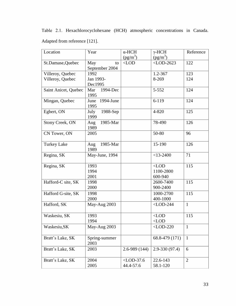
Rocky mountains [111-113]. Table 2.1 shows that the highest atmospheric concentrations

of γ-HCH in the 1990’s to 2001 were observed at sampling sites in Saskatchewan

including Regina and Hafford with maximum atmospheric concentrations of γ-HCH in

excess of 2000 pg/m3

[115]. These sites were within a region of heavy canola cultivation.

High atmospheric concentrations (>1000 pg/m3) were also reported in Alberta [116].

Table 2.2 shows these atmospheric concentrations of γ-HCH in Saskatchewan were

similar to other countries such as France when usage of lindane during this time period

was >100 t/yr [117- 119]. High concentrations of -HCH (400-650 pg/m3) have also been

measured in Paris, France [12]. Passive air sampling in 2000-2001 across North America

also showed that Canadian prairies had the highest levels of γ-HCH and the lowest ratio

of α/γ-HCH (ratio =0.2) [120].

33

Table 2.1. Hexachlorocyclohexane (HCH) atmospheric concentrations in Canada.

Adapted from reference [121].

Location Year α-HCH

(pg/m3)

γ-HCH

(pg/m3)

Reference

St.Damase,Quebec May to

September 2004

<LOD

<LOD-2623

122

Villeroy, Quebec

Villeroy, Quebec

1992

Jan 1993-

Dec1995

1.2-367

8-269

123

124

Saint Anicet, Quebec Mar 1994-Dec

1995

5-552 124

Mingan, Quebec June 1994-June

1995

6-119 124

Egbert, ON July 1988-Sep

1999

4-820 125

Stony Creek, ON Aug 1985-Mar

1989

78-490 126

CN Tower, ON

2005 50-80 96

Turkey Lake Aug 1985-Mar

1989

15-190 126

Regina, SK

May-June, 1994 <13-2400 71

Regina, SK 1993

1994

2001

<LOD

1100-2800

600-940

115

Hafford-C site, SK

1998

2000

2600-7400

900-2400

115

Hafford G-site, SK 1998

2000

1000-2700

400-1000

115

Hafford, SK

May-Aug 2003 <LOD-244 1

Waskesiu, SK 1993

1994

<LOD

<LOD

115

Waskesiu,SK

May-Aug 2003 <LOD-220 1

Bratt’s Lake, SK Spring-summer

2003

68.8-479 (171) 1

Bratt’s Lake, SK

2003 2.6-989 (144) 2.9-330 (97.4) 6

Bratt’s Lake, SK

2004

2005

<LOD-37.6

44.4-57.6

22.6-143

58.1-120

2

34

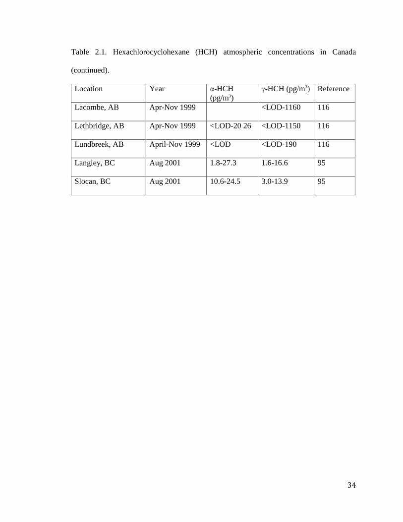
Table 2.1. Hexachlorocyclohexane (HCH) atmospheric concentrations in Canada

(continued).

Location Year α-HCH

(pg/m3)

γ-HCH (pg/m3) Reference

Lacombe, AB

Apr-Nov 1999 <LOD-1160 116

Lethbridge, AB

Apr-Nov 1999 <LOD-20 26 <LOD-1150 116

Lundbreek, AB

April-Nov 1999 <LOD <LOD-190 116

Langley, BC

Aug 2001 1.8-27.3 1.6-16.6 95

Slocan, BC

Aug 2001 10.6-24.5 3.0-13.9 95

35

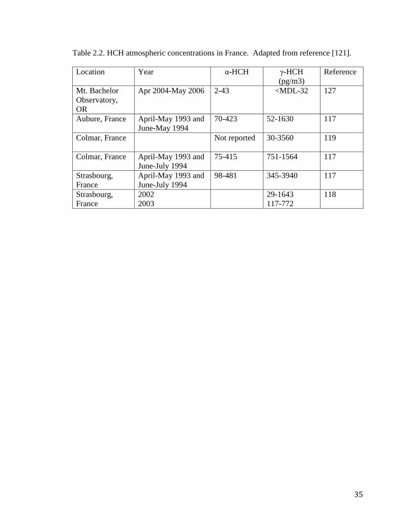
Table 2.2. HCH atmospheric concentrations in France. Adapted from reference [121].

Location Year α-HCH γ-HCH

(pg/m3)

Reference

Mt. Bachelor

Observatory,

OR

Apr 2004-May 2006 2-43 <MDL-32 127

Aubure, France April-May 1993 and

June-May 1994

70-423 52-1630 117

Colmar, France

Not reported 30-3560 119

Colmar, France April-May 1993 and

June-July 1994

75-415 751-1564 117

Strasbourg,

France

April-May 1993 and

June-July 1994

98-481 345-3940 117

Strasbourg,

France

2002

2003

29-1643

117-772

118

36

In 2003, the last year of reported usage of lindane in Saskatchewan, a significant

reduction in atmospheric concentrations of γ-HCH at Bratt’s Lake (located within 35 km

of Regina where previous measurements had been taken) was observed with maximum

concentrations <500 pg/m3

and a number of sampling periods observed concentrations

less than LOD of 1 pg/m3. The detection frequency of samples collected from April 2003-

March 2004 for and γ-HCH was 32% and 29%, respectively [6]. Studies by our

research group at Bratt’s Lake in 2003 had short duration sampling (<1 week) [20]. This

sampling by Dr. Hall showed that α-HCH was present and could reach or exceed

atmospheric concentrations observed for γ-HCH (maximum HCH 989 pg/m3, γ-HCH

312 pg/m3) [6]. During May and June 2003 when both and γ- HCH were observed

>LOD, the ratio of /-HCH ranged from 1.1-4.4 (average 2.1) which was significantly

higher than reported from passive sampling in 2000-2001 [120]. There was indication

that significant aging of γ-HCH has occurred along with some periods of regional or local

application of remaining stocks of lindane influencing atmospheric concentrations.

Atmospheric concentrations of γ-HCH continued to decline in 2004 and 2005 at Bratt’s

Lake, SK following the removal of lindane products from usage (see Table 2.1). Long-

term trend analysis for Alert site in the Canadian Arctic also showed declining γ-HCH

concentrations in the atmosphere during this time period [128-130]. In the Pacific

Northwest region of North America at Mt. Bachelor Observatory, OR and sites in British

Columbia in early 2000’s atmospheric concentrations of HCHs were significantly lower

than in the Canadian Prairies [95, 114, 127]. In the Lower Frazer Valley, BC at a rural

site (Langley) and urban site (Slocan) concentrations of HCHs during sampling in 2000-

2001 were <30 pg/m3 (see Table 2.1) and at Mt. Bachelor atmospheric concentrations of

37

and -HCH were less than 45 pg/m3

[39].

HCHs can be detected in the atmosphere in other countries. For example, HCHs

were found in the air in Senga Bay on the southwest shore of Lake Malawi, in southeast

Africa. The maximum air concentration was 10 pg/m3

for -HCH and 176 pg/m3

for -

HCH [106]. The ratio of -HCH/-HCH for the sampling periods of May 29th

and June

21st was 0.05 indicating a source of lindane contributed to atmospheric loadings of HCHs

in the atmosphere [106].

Chlorpyrifos is the main organophosphorus pesticide used for insect control in

Saskatchewan and was chosen for further study in this thesis research. It can be analyzed

by GC/MS along with OCs. Chlorpyrifos is used in Saskatchewan and the prairies

predominately for grasshopper control on a wide variety of crops including canola,

wheat, barley, oats, flax, lentils, sunflowers, and potatoes [4, 5]. In 1996, chlorpyrifos

was detected in the atmosphere in Abbotsford, BC in the summer and fall with average

concentrations at 303 pg/m3 in early July and at 753 pg/m

3 in the end of October [131].

The maximum concentration of chlorpyrifos was detected in the end of September at

1500 pg/m3

[131]. In 2005, atmospheric concentrations of chlorpyrifos were lower at

Abbotsford, BC (chlorpyrifos 3.9-86.7 pg/m3, chlorpyrifos oxon <LOD to 3.2-186 pg/m

3)

[19]. Atmospheric concentrations of diazinon and malathion are much higher than

chlorpyrifos at Abbotsford due to their use on berry crops [19]. In 2005 at Bratt’s Lake,

SK atmospheric concentrations of chlorpyrifos ranged from 0.6-1380 pg/m3 and

chlorpyrifos oxon <LOD to 3900 pg/m3 [19]. Atmospheric concentrations of chlorpyrifos

at Bratt’s Lake, SK were also much higher in 2003 (233000 pg/m3) than in 2005 (1380

pg/m3) and were associated with higher usage of chlorpyrifos in 2003 due to the large

38

numbers of grasshopper’s at Bratt’s Lake and southern Saskatchewan [6, 19]. In 2005,

the atmospheric concentrations of chlorpyrifos were also much higher at Bratt’s Lake, SK

than observed at Abbotsford, BC [19]. Between 1994 and 1996, high atmospheric

concentrations of chlorpyrifos were also reported (10000-103000 pg/m3) in Manitoba in

the South Tobacco Creek Watershed [132]. This sampling in Manitoba occurred during a

period of local applications of pesticides (late July and mid-August of each sampling

year). Detectable atmospheric concentrations of chlorpyrifos (0.4-4.6 pg/m3) were also

reported in the Canadian Rocky Mountains where there is no local usage [104, 133].

Chlorpyrifos has also been used in urban and agricultural areas of the United

States. In 1995, chlorpyrifos was detected in air samples from an urban and an

agricultural sampling site in Mississippi. Chlorpyrifos is the most frequently detected

pesticides in both agricultural and urban site in Mississippi and it is primarily detected in

the gas phase in air. Chlorpyrifos maximum air concentrations at urban and agricultural

sites were 3500 pg/m3

(September 1995) and 3100 pg/m3, respectively [134]. High

atmospheric concentrations in urban areas were attributed to usage of chlorpyrifos for fire

ant and termite control in urban areas [134]. Atmospheric concentrations in agricultural

areas were influenced by atmospheric transport from urban sources. Urban, suburban,

and rural measurements were made in eastern Iowa, U.S. during June 2001-2002. The

highest median atmospheric concentration of chlorpyrifos during June 2001-2002 was

reported at the suburban site (1400 pg/m3), while at the rural location median

concentration were below the method detection limit (maximum concentration of 880

pg/m3) [135]. This showed the importance of residential and commercial use of

chlorpyrifos in the early 2000’s in the United States. California had significant usage of

39

chlorpyrifos on crops such as citrus fruit and nuts [136]. The concentrations of

chlorpyrifos were also determined in air along the Mississippi River during the first 10

days of June 1994. The maximum concentration of chlorpyrifos was 1600 pg/m3 [137].

The presence of chlorpyrifos in the atmosphere was associated with the expected usage of

a wide variety of insecticides on cropland in the Mississippi River [137].

Chlorpyrifos concentrations in the air were detected from April 17 through June

26, 1995 in the Chesapeake Bay watershed a study site on the Patuxent River in

Solomons, MD, in Northeastern United States. The concentrations of chlorpyrifos were

ranged from 15 to 2000 pg/m3

with a mean air concentration of 200 pg/m3. This study

showed the air concentrations of chlorpyrifos were very low during the early spring and

then increased in late May to early June as a result of regional usage of chlorpyrifos and

also increased with air temperatures. With higher temperatures, higher volatilization

rates of chlorpyrifos in the air are expected [100]. Similar, seasonal variations of

chlorpyrifos have also been reported at Bratt’s Lake, SK [19].

OPs have been used widely in California. During the summer of 1996

atmospheric concentrations of chlorpyrifos reached 17500 pg/m3

in June at the Kaweah

Reservoir, a low elevation sampling site located near Sequoia National Park, California

where there is no local usage of chlorpyrifos [98]. This high atmospheric concentration

of chlorpyrifos was consistent with the expected agricultural usage of chlorpyrifos in the

summer in the California Central Valley [98]. Concentrations of chlorpyrifos oxon were

also reported to be the highest in May at 30400 pg/m3

[98]. Chlorpyrifos was also the

most frequently detected pesticide in air in the Sierra Nevada Mountain Range [138].

Other studies in mountain ranges have also detected chlorpyrifos in the atmosphere.

40

Chlorpyrifos was detected in the atmosphere in two National Parks in Brazilian

southeastern and southern mountain regions during 2007-2008 with air concentrations

ranged 4-35 and 15-130 pg/m3, respectively [104].

In 2009 in the Valencia Region of Spain high concentrations of chlorpyrifos were

observed (ranging from 29100-1428 pg/m3) [79]. The concentrations of chlorpyrifos

were also measured in 2010 at the same site and at additional sites including one remote

site (Morella), and three rural sites (Alzira, Burriana, and Sant Jordi). The highest mean

concentrations of chlorpyrifos were obtained at rural sites, Alzira (17.69 pg/m3) and

Burriana (14.76 pg/m3) [139]. Concentrations of chlorpyrifos in Morella, Sant Jordi and

Valencia were found in similar average concentrations at 12.5, 10.8 and 10.1 pg/m3,

respectively [139]. Each site showed different seasonal variations that were related to the

different types of crops in the vicinity of the sampling site. Atmospheric concentrations

of pesticides in the rural sites were linked to the agricultural practices nearby. At the

urban site, the pesticides were detected as a result of their use in gardening in residential

areas as well as potential atmospheric transport from nearby rural areas. Other factors,

such as application during the sampling period, wind speed or degradation processes were

suggested to influence atmospheric concentrations of chlorpyrifos [139].

Based on 2003 usage information for Canada [18, 109] >90%-100% of the usage

of pre-emergent herbicides is in the prairie provinces of Canada. The prairie provinces

accounted for ∼94% of usage of trifluralin in Canada in 2003 [18, 109]. Trifluralin is

also used on a wide variety of crops in Canada with usage also in Ontario, Quebec,

British Columbia, Nova Scotia, and New Brunswick [18]. In 2003, other regions of

Canada had low or no reported usage of triallate and ethalfluralin, [18] with previous

41

measurements in these regions generally showing atmospheric concentrations of triallate

and ethalfluralin < LOD [1, 7, 131]. Table 2.3 shows that the highest atmospheric

concentrations of trifluralin in the atmosphere were observed in Saskatchewan. A

maximum of 62000 pg/m3 was reported in Melfort, SK located in northwestern region of

the province outside of the soil zones with expected highest usage of pre-emergent

herbicides giving strong evidence for atmospheric transport potential [140]. At Bratt’s

Lake, SK and study sites nearby where pre-emergent herbicides were used locally and

regionally in agricultural areas, maximum atmospheric concentrations of trifluralin were

generally 2000-3600 pg/m3 for air samples collected from 1989 through 2005 (see Table

2.3). Bratt’s Lake, SK and other Saskatchewan sites had the highest reported

atmospheric concentrations of trifluralin during 1990-2005 in Canada [2, 7, 141, 142].

Passive air sampling of trifluralin at 20 sites operated under the GAPS (Global

Atmospheric Passive Sampling) Network also shows the highest atmospheric

concentrations of trifluralin at Bratt’s Lake, SK [143]. Table 2.4 shows that atmospheric

concentrations >2000 pg/m3 have been reported in other agricultural regions outside of

Canada with significant usage of trifluralin such as France and United States (Minnesota,

Iowa). The presence of trifluralin in France was associated with its use in the agriculture

areas [144]. Trifluralin was also detected in urban, rural, and suburban sites in eastern

Iowa during 2000-2002, with average concentration of 520 pg/m3 and a maximum

concentration of 8200 pg/m3 [135]. In Saskatchewan where measurements at Bratt’s

Lake and Regina (within 35 km distance) exist for a number of years the atmospheric

concentration ranges can vary on an annual basis but remained high in 2003 and 2005

(see Table 2.3). High concentrations of trifluralin (>1000 pg/m3) have also been

42

observed in Ontario (Egbert in 1989), Quebec (St. Damase), and British Columbia

(Abbotsford) where there has been reported usage of trifluralin [18].

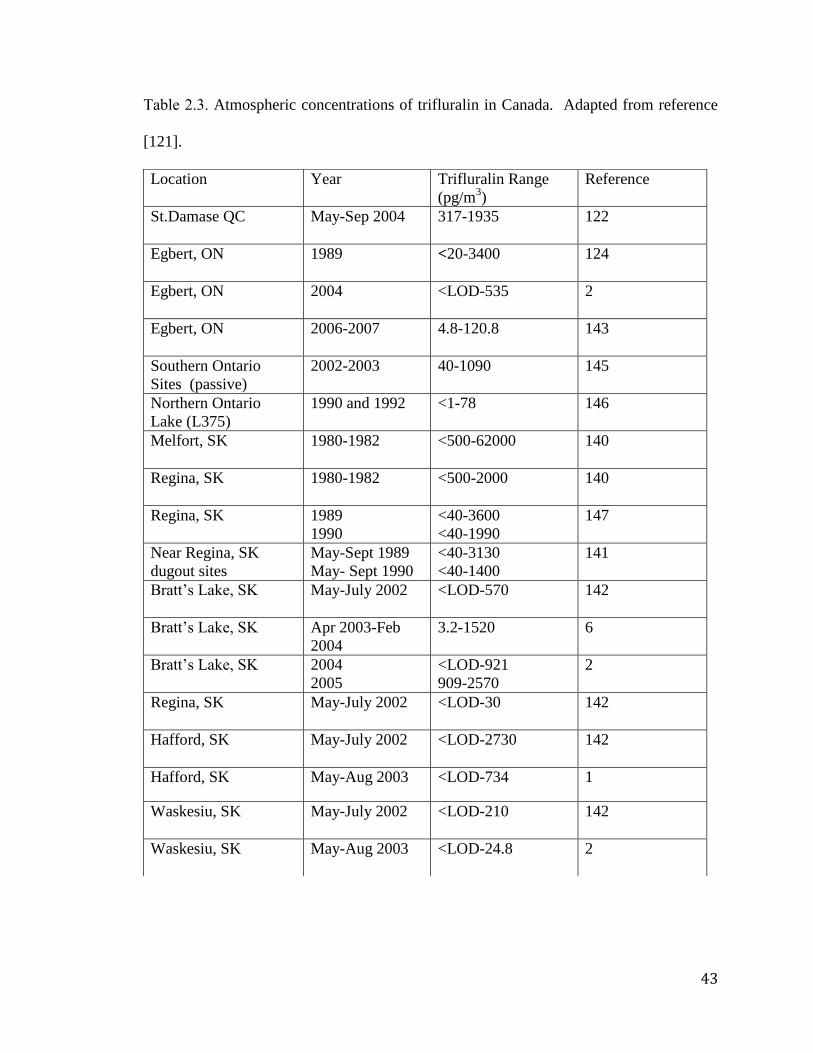
43

Table 2.3. Atmospheric concentrations of trifluralin in Canada. Adapted from reference

[121].

Location Year Trifluralin Range

(pg/m3)

Reference

St.Damase QC

May-Sep 2004 317-1935 122

Egbert, ON

1989 <20-3400 124

Egbert, ON

2004 <LOD-535 2

Egbert, ON

2006-2007 4.8-120.8 143

Southern Ontario

Sites (passive)

2002-2003 40-1090 145

Northern Ontario

Lake (L375)

1990 and 1992 <1-78 146

Melfort, SK

1980-1982 <500-62000 140

Regina, SK

1980-1982 <500-2000 140

Regina, SK 1989

1990

<40-3600

<40-1990

147

Near Regina, SK

dugout sites

May-Sept 1989

May- Sept 1990

<40-3130

<40-1400

141

Bratt’s Lake, SK

May-July 2002 <LOD-570 142

Bratt’s Lake, SK

Apr 2003-Feb

2004

3.2-1520 6

Bratt’s Lake, SK

2004

2005

<LOD-921

909-2570

2

Regina, SK

May-July 2002 <LOD-30 142

Hafford, SK

May-July 2002 <LOD-2730 142

Hafford, SK

May-Aug 2003 <LOD-734 1

Waskesiu, SK

May-July 2002 <LOD-210 142

Waskesiu, SK

May-Aug 2003 <LOD-24.8 2

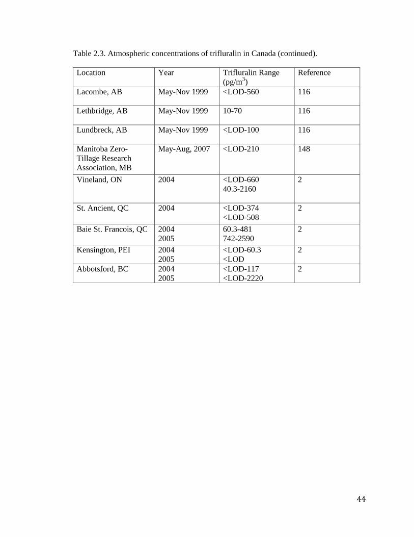
44

Table 2.3. Atmospheric concentrations of trifluralin in Canada (continued).

Location Year Trifluralin Range

(pg/m3)

Reference

Lacombe, AB

May-Nov 1999 <LOD-560 116

Lethbridge, AB

May-Nov 1999 10-70 116

Lundbreck, AB

May-Nov 1999 <LOD-100 116

Manitoba Zero-

Tillage Research

Association, MB

May-Aug, 2007

<LOD-210 148

Vineland, ON

2004

<LOD-660

40.3-2160

2

St. Ancient, QC 2004 <LOD-374

<LOD-508

2

Baie St. Francois, QC 2004

2005

60.3-481

742-2590

2

Kensington, PEI 2004

2005

<LOD-60.3

<LOD

2

Abbotsford, BC 2004

2005

<LOD-117

<LOD-2220

2

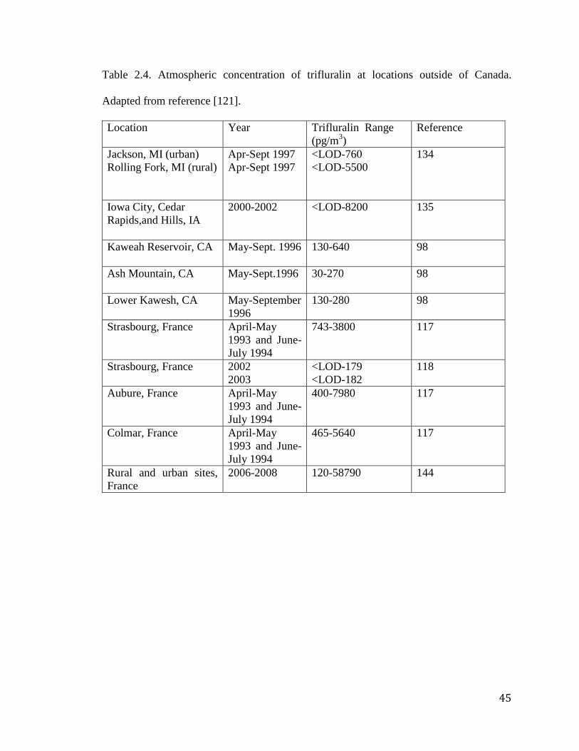
45

Table 2.4. Atmospheric concentration of trifluralin at locations outside of Canada.

Adapted from reference [121].

Location Year Trifluralin Range

(pg/m3)

Reference

Jackson, MI (urban)

Rolling Fork, MI (rural)

Apr-Sept 1997

Apr-Sept 1997

<LOD-760

<LOD-5500

134

Iowa City, Cedar

Rapids,and Hills, IA

2000-2002 <LOD-8200 135

Kaweah Reservoir, CA

May-Sept. 1996 130-640 98

Ash Mountain, CA

May-Sept.1996 30-270 98

Lower Kawesh, CA May-September

1996

130-280 98

Strasbourg, France

April-May

1993 and June-

July 1994

743-3800 117

Strasbourg, France

2002

2003

<LOD-179

<LOD-182

118

Aubure, France

April-May

1993 and June-

July 1994

400-7980 117

Colmar, France

April-May

1993 and June-

July 1994

465-5640 117

Rural and urban sites,

France

2006-2008 120-58790 144

46

There are limited studies that have reported concentrations > LOD for triallate and

ethalfluralin. The highest atmospheric concentrations of triallate at Bratt’s Lake during

2002-2005 were reported in 2003, and were similar in magnitude to maximum

atmospheric concentrations of triallate reported near Regina at farm dugout sites in prior

years (see Table 2.5). Maximum concentrations of triallate at these sites in Saskatchewan

often ranged between 10,000 and 60,000 pg/m3 and were much higher than those reported

for trifluralin. Maximum atmospheric concentrations of triallate were highest in the late

1990s and prior to 2004. Table 2.5 shows that lower atmospheric concentrations of

triallate were observed in Alberta than Saskatchewan. Mixed granular formulation

containing triallate and trifluralin are also not recommended for use in Manitoba [108].

Lower usage of triallate has also been reported since 2003 in Canada, Alberta and

Manitoba [111, 148-151]. Atmospheric concentrations of ethalfluralin were only

available for Bratt’s Lake during 2003-2005, with the highest concentrations in 2005

when a maximum of 7570 pg/m3

was reported (see Table 2.5). Atmospheric

concentrations of ethalfluralin are generally lower in other prairie provinces.

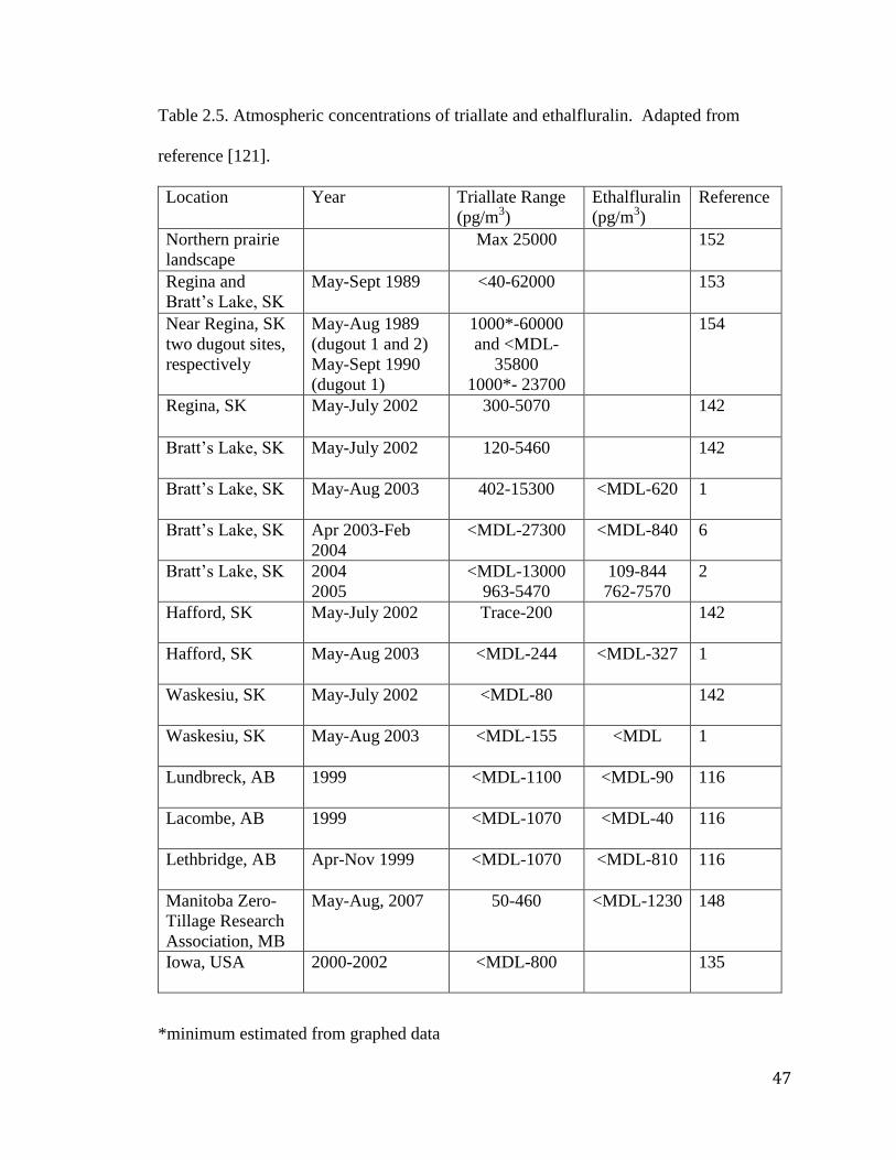
47

Table 2.5. Atmospheric concentrations of triallate and ethalfluralin. Adapted from

reference [121].

Location Year Triallate Range

(pg/m3)

Ethalfluralin

(pg/m3)

Reference

Northern prairie

landscape

Max 25000 152

Regina and

Bratt’s Lake, SK

May-Sept 1989 <40-62000 153

Near Regina, SK

two dugout sites,

respectively

May-Aug 1989

(dugout 1 and 2)

May-Sept 1990

(dugout 1)

1000*-60000

and <MDL-

35800

1000*- 23700

154

Regina, SK

May-July 2002 300-5070 142

Bratt’s Lake, SK

May-July 2002 120-5460 142

Bratt’s Lake, SK

May-Aug 2003 402-15300 <MDL-620 1

Bratt’s Lake, SK Apr 2003-Feb

2004

<MDL-27300 <MDL-840 6

Bratt’s Lake, SK 2004

2005

<MDL-13000

963-5470

109-844

762-7570

2

Hafford, SK

May-July 2002 Trace-200 142

Hafford, SK

May-Aug 2003 <MDL-244 <MDL-327 1

Waskesiu, SK

May-July 2002 <MDL-80 142

Waskesiu, SK

May-Aug 2003 <MDL-155 <MDL 1

Lundbreck, AB

1999 <MDL-1100 <MDL-90 116

Lacombe, AB

1999 <MDL-1070 <MDL-40 116

Lethbridge, AB

Apr-Nov 1999 <MDL-1070 <MDL-810 116

Manitoba Zero-

Tillage Research

Association, MB

May-Aug, 2007 50-460 <MDL-1230 148

Iowa, USA

2000-2002 <MDL-800 135

*minimum estimated from graphed data

48

2.3 Pesticide usage and formulation information

A provincial based inventory for pesticide usage for the agriculture sector is

available in Canada for 2003, and on a gridded basis in the United States through the

Pesticide National Synthesis Project for 2002 [18, 109, 136]. World and US market

expenditure estimates have shown that herbicides comprise the largest fraction of

pesticide usage. Total pesticide usage has increased since 2002 world-wide and in the

United States primarily due to increased use of fungicides and insecticides [155]. In

United States, total herbicide usage increased in the 1990s, and since 2002 there has been

a small decline [115]. Trifluralin was ranked the 17th

most commonly used conventional

pesticide in the United States with its usage declining (2001, 2003, 2005, and 2007 usage

range of 5.4-7.3, 3.6-4.5, 3.2-4.1, 2.3-3.2 million kg of active ingredient, respectively)

[115]. Triallate and ethalfluralin were not listed in the top 20 pesticides for the United

States [115] and based on 2002 were 20% of usage of trifluralin [136]. More than 99%

of triallate and ethalfluralin in Canada occurred in the Canadian prairies [18, 109].

Trifluralin was used on a larger variety of crops in the United States than Canada with

dominate usage in Canada on grain and oil seed crops in the prairies [18, 109]. Canadian

usage of trifluralin, ethalfluralin, and triallate in 2003 were estimated at 0.37, 0.64, and

0.75 million of kg of active ingredient, respectively [18, 109]. Ethalfluralin and triallate

remained in the top 10 active ingredients sold in Canada in 2008 with annual usage of

ethalfluralin >0.5-1.0 million kg, and triallate and trifluralin usage was >0.1-0.5 million

kg [149]. Triallate has shown the largest reduction in usage between 2003 and 2008

particularly in the province of Alberta where annual usage declined from 0.2 to 0.1

million kg [150]. Canadian annual usage of pesticides has increased from 9.3 to 12.5

49

million kg from 2003 to 2008 [149]. The prairie provinces comprise of 60% of usage of

pesticides in Canada with Saskatchewan having the highest provincial usage [18].

Saskatchewan pesticide sales also increased from 2001 to 2003 (see Figure 2.1 for pre-

emergent herbicides). Annual average usages between 2004-2006 in Manitoba for

ethalfluralin, trifluralin, and triallate were 93100, 41700, and 7200 kg, respectively [148].

Similar pesticide usage in 2010 and 2011 is Manitoba has been reported, although

expenditures dropped due to lower cost of gylphosate in 2011 [156]. Pesticide usage in

the prairie provinces is dominated by herbicides such as glyphosate, pre-emergent

herbicides (triallate, trifluralin, ethalfluralin), and acid herbicides (2,4-D, MCPA,

dichlorprop,dicamba, and bromoxynil). Glyphosate has seen the largest increases in

herbicide usage in the prairies provinces particularly for canola and this is expected to

continue with its low cost [148, 149, 156]. With the rise of herbicide resistant weeds in

the prairies, the rotation of herbicides and mixed herbicide applications has become

important including the use of the pre-emergent herbicides in combination with other

pesticides [157, 158].

In 1990, Canada, France, Italy, Niger, Honduras, the United States, and China

were the leading lindane consuming countries with Canada’s usage in 1980 and 1990 at

286 t/yr and 284.5 t/yr, respectively [110]. Historically, lindane was widely used as an

insecticide on canola and wheat crops. Usage of lindane for canola seed treatment in the

prairie region in 1997 and 1998 was estimated at 445.3 and 510.4 t/yr, respectively [72]

showing that agricultural usage in 2001-2003 (see Figure 2.1 A) during the time of its

restrictions was significantly less than prior to 2000. Figure 2.1 B will be discussed in

more detail in the result and discussion section.

50

0

500

1000

1500

2000

2500

Dark Brown Soil Zone Brown Soil Zone Total SK

Usag

e (kg

)

A2001

2002

2003

0

50000

100000

150000

200000

Usag

e (kg

)

B

2001

2002

2003

Figure 2.1. Usage of selected pesticides in Saskatchewan during 2001-2003. A, Lindane;

B, pre-emergent herbicides. Brackets are used to note soil zones of major pesticide usage

in B. Data source: Government of Saskatchewan, Saskatchewan Agriculture and Food,

unpublished data [109].

51

In 2003 highest usage of chlorpyrifos in Canada was reported in the prairie

provinces with usage in Alberta and Saskatchewan (>200,000 kg provincial usage) and

significantly greater than in Manitoba [5, 75]. Usage of chlorpyrifos also varies

significantly annually with usage of chlorpyrifos in Saskatchewan in 2001, 2002, and

2003 of 7267 Kg, 121,824 Kg, and 205,562 Kg, respectively [5].

In 2002 base pesticide usage maps for the United States, triallate was primarily

used in North Dakota and Montana for weed control for wheat and barley; trifluralin was

used on a wider range of crops (soybeans, cotton, alfalfa hay, and wheat) with its main

usage in North Dakota, Minnesota, and Iowa; and ethalfluralin was mainly used in the

Dakotas and northwest corner of Minnesota with the highest US usage on sunflower

seeds, dry beans, peanuts, and soybeans [136]. Chlorpyrifos can also be used on

soybeans and wheat in the Dakotas and northwest corner of Minnesota, and was also

commonly used on corn in the United States [136].

52

3. EXPERMENTAL

3.1 Materials

Acetone, ethyl acetate, hexane and methanol were pesticide grade and supplied by

Fisher Scientific (Ottawa, ON, Canada). Individual pesticide standards and deuterated

internal standards (parathion-d10 and chlorpyrifos-d10) were supplied by Chem Service

Inc. (West Chester, PA). Stock solutions of individual standards were prepared in

acetone at 1.0 mg/mL for subsequent dilution. Standard mixtures at 1.0 µg/mL were

prepared in pesticide grade hexane. Calibration standards were prepared from 0.1 pg/L

to 100 or 200 pg/L with final concentration of internal standards, parathion-d10 25 L of

10 pg/L, in all standards and samples. All final diluted standards were prepared on the

day of analysis. Polyurethane foam (PUF) plugs (2.54 cm, 5.08 cm, 7.62 cm lengths) and

glass fibre filters (10.2 cm diameter) were purchased from Pacwill Environmental

(Grimsby, ON, Canada). Labx 170 cleanroom filters (10.16 cm diameter, 63% abaca,

37% softwood with polymeric binders) were purchased from Berkshire (Great

Barrington, MA). The granular sorbents XAD-2 and XAD-4 were obtained from Supelco

Inc. (Oakville, ON, Canada). All PUF and sorbent materials were cleaned prior to

sampling with the same pressurized solvent extraction method described in the extraction

procedure. To remove any residual organics that may have absorbed during shipping of

new filters, the Labx 170 filters were placed in an oven typically for >8 hours or

overnight at 100 C.

53

3.2 Site description and collection of atmospheric samples

The sampling site at Bratt’s Lake, SK is an Environment Canada operated field site

in the prairie agricultural region where grain and oil seeds such as wheat, barley, oats,

canola and flax are predominant. Other specialty crops like lentils and peas are also

grown. The station is located approximately 35 km southwest of Regina, SK, Canada.

The approximate location of the Bratt’s Lake site is shown on the soil zone map in Figure

3.1. Agriculture Saskatchewan describes Bratt’s Lake as being in the dark brown soil

region [159]. Bratt’s Lake sampling site is located in rural municipality #129 Bratt’s

Lake. The coordinates of the site are: latitude: 50º16’ N, longitude: 104º42’ W. Air

samples were collected continuously at Bratt’s Lake, Saskatchewan in 2007-2010 with a

PS-1 high-volume air sampler (Tisch Environmental, Cleves, OH) with typical air

volumes of 2500 m3

for a sampling duration of 7-days (operated continuously).

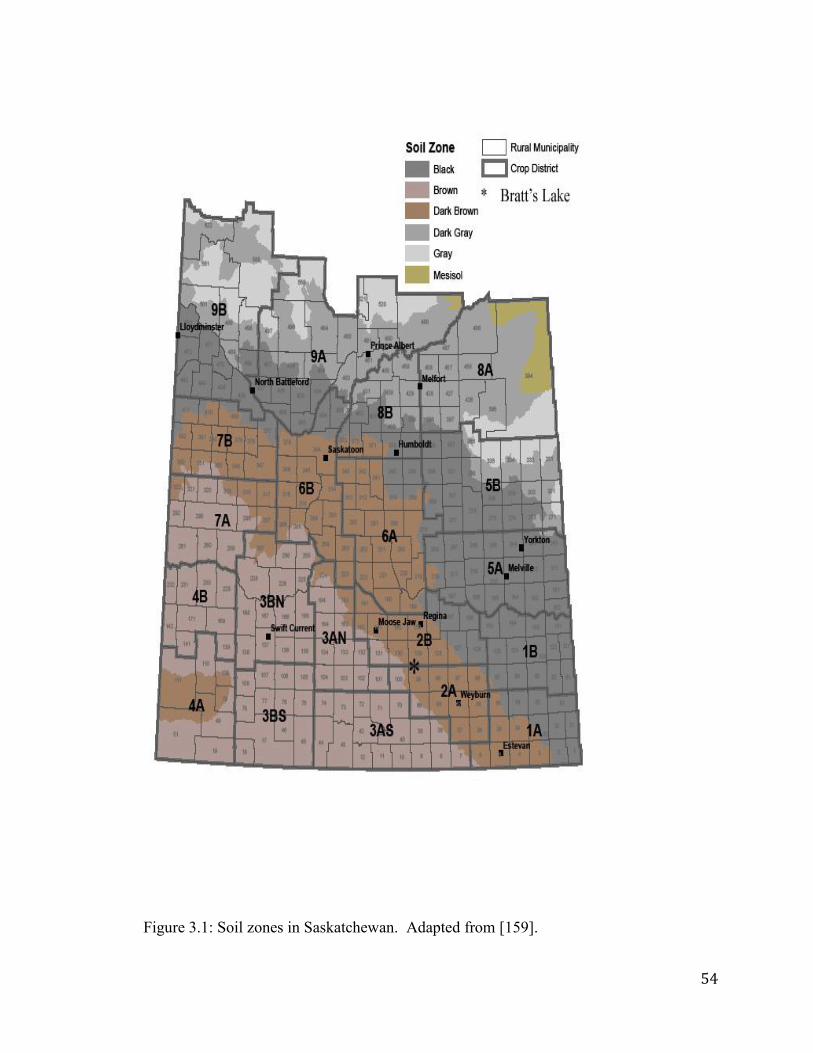
54

Figure 3.1: Soil zones in Saskatchewan. Adapted from [159].

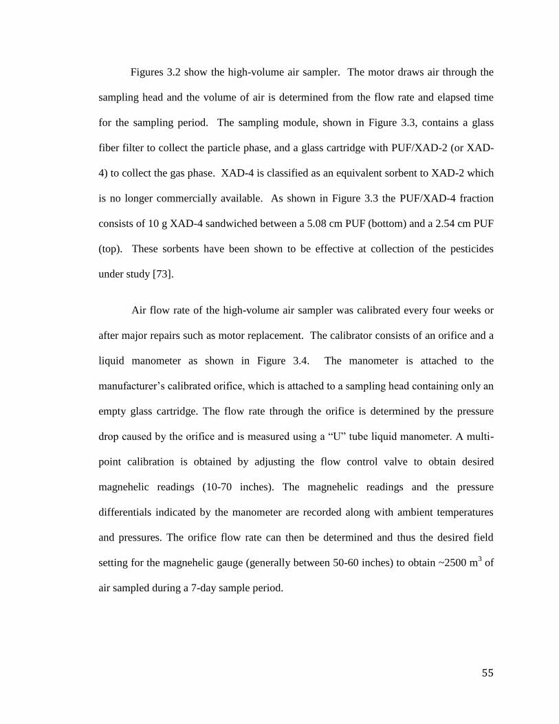
55

Figures 3.2 show the high-volume air sampler. The motor draws air through the

sampling head and the volume of air is determined from the flow rate and elapsed time

for the sampling period. The sampling module, shown in Figure 3.3, contains a glass

fiber filter to collect the particle phase, and a glass cartridge with PUF/XAD-2 (or XAD-

4) to collect the gas phase. XAD-4 is classified as an equivalent sorbent to XAD-2 which

is no longer commercially available. As shown in Figure 3.3 the PUF/XAD-4 fraction

consists of 10 g XAD-4 sandwiched between a 5.08 cm PUF (bottom) and a 2.54 cm PUF

(top). These sorbents have been shown to be effective at collection of the pesticides

under study [73].

Air flow rate of the high-volume air sampler was calibrated every four weeks or

after major repairs such as motor replacement. The calibrator consists of an orifice and a

liquid manometer as shown in Figure 3.4. The manometer is attached to the

manufacturer’s calibrated orifice, which is attached to a sampling head containing only an

empty glass cartridge. The flow rate through the orifice is determined by the pressure

drop caused by the orifice and is measured using a “U” tube liquid manometer. A multi-

point calibration is obtained by adjusting the flow control valve to obtain desired

magnehelic readings (10-70 inches). The magnehelic readings and the pressure

differentials indicated by the manometer are recorded along with ambient temperatures

and pressures. The orifice flow rate can then be determined and thus the desired field

setting for the magnehelic gauge (generally between 50-60 inches) to obtain ~2500 m3 of

air sampled during a 7-day sample period.

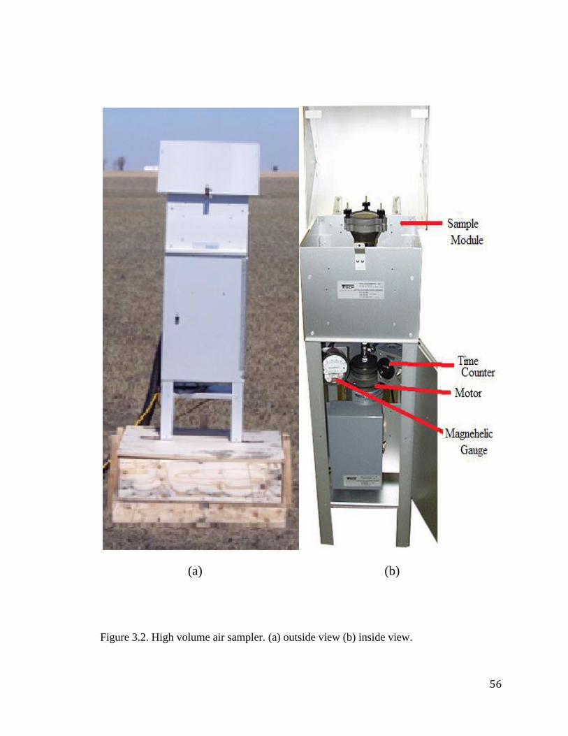
56

(a) (b)

Figure 3.2. High volume air sampler. (a) outside view (b) inside view.

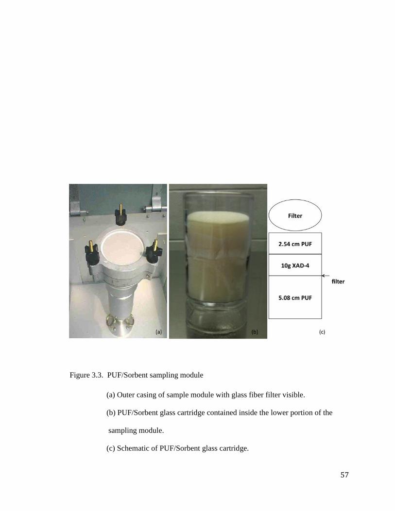
57

Figure 3.3. PUF/Sorbent sampling module

(a) Outer casing of sample module with glass fiber filter visible.

(b) PUF/Sorbent glass cartridge contained inside the lower portion of the

sampling module.

(c) Schematic of PUF/Sorbent glass cartridge.

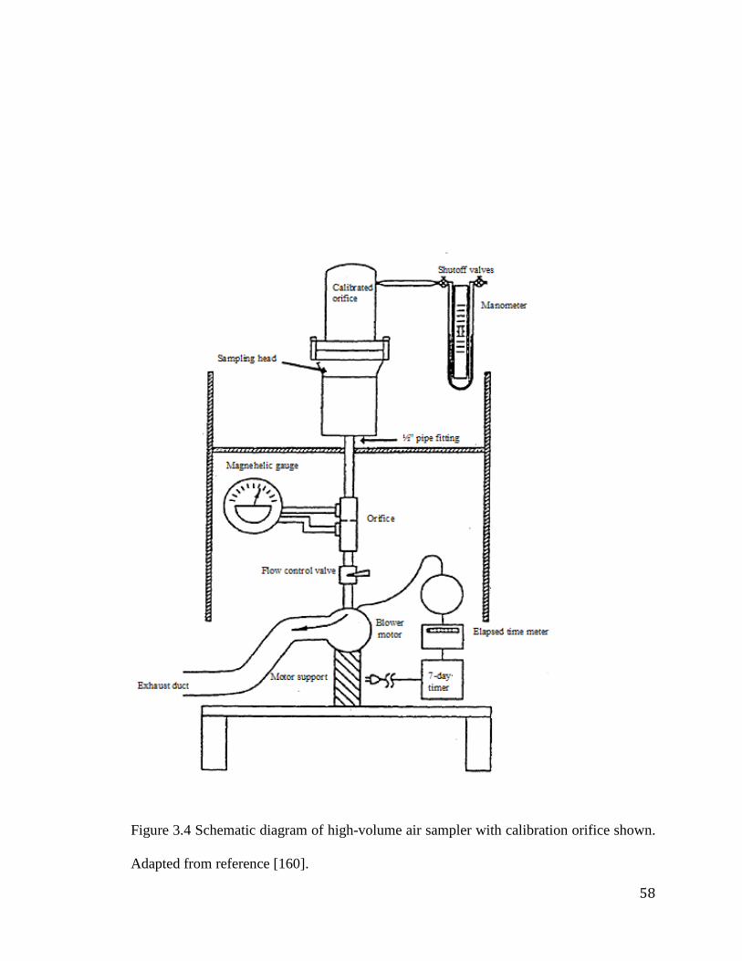
58

Figure 3.4 Schematic diagram of high-volume air sampler with calibration orifice shown.

Adapted from reference [160].

59

3.3 Filter analysis

Glass fibre filters were weighed (± 1.5 µg) before and after sampling using a

microbalance (Mettler Toledo, Mississauga, ON, Canada) in a glove box with a nitrogen

atmosphere for humidity control. Filters were conditioned for 24 hours in the glove box

atmosphere prior to weighing both before and after sampling. The difference in mass

between the before and after measurements was the mass of particles collected. The

particle concentration was calculated by dividing the mass of particles by the air volume

for the sampling period.

3.4 Pressurized solvent extraction

As this research only involved the gas phase fraction of collected samples, after

sampling, the PUFs and sorbents (7.62 cm PUF, sorbents) were extracted together in 100

mL extraction cell using ethyl acetate with an ASE100 or ASE300 pressurized solvent

extraction system (Dionex, Sunnyvale, CA). The extraction method parameters were:

temperature, 100 ºC; static mode time, 30 min at 1500 psi; two static cycles; 60% flush

volume; purge time with ultra high purity (UHP) nitrogen of 300 s. The total extraction

volume was approximately 150 mL for a 100 mL extraction cell [19, 20]. The sampling

materials (PUFs and sorbents) were also cleaned with a Soxhlet extraction with ethyl

acetate as the extraction solvent. All sample extractions (after sampling) were done using

pressurized solvent extraction using ethyl acetate.

After extraction, samples were concentrated to 5-10 mL by blow down with

nitrogen or cleanroom air using a solid phase extraction (SPE) apparatus (Supelco Inc.,

Oakville, ON, Canada). After the volume was reduced, samples were transferred to 10

60

mL vials and blown down further to 100 L under the same conditions. Prior to

cleanup, the samples were re-dissolved in 1 mL of methanol.

3.5 Sample cleanup using solid phase extraction

C18 (ENVI-18, 6 mL, 1 g, Supelco Inc., Oakville, ON, Canada) SPE tubes were

used and conditioned with 6 mL ethyl acetate, followed by 6 mL methanol. Sample

extract (0.25 mL) was loaded onto the preconditioned SPE tubes, followed by surrogate

standard (50 L of 10 g/mL diazinon-d10) and methanol such that the total volume was

1 mL. The eluted solvent collected into fraction (F0) was observed to contain no

pesticides of interest. The pesticides were eluted with 5 mL ethyl acetate in the next

fraction (F1), and the Versiprep drying attachment (Supelco) was used to evaporate and

concentrate eluted extracts from SPE (and from ASE) to 100 L volume. These extracts

from SPE were re-dissolved with 1mL hexane. Parathion-d10 (or chlorpyrifos-d10) was

used as the internal standard, while diazinon-d10 was used as the surrogate standard. A 25

µL volume of internal standard (10 µg/mL) was added to all samples and standards

prepared for GC-MS analysis.

3.6 Instrumental analysis

The GC/MS system consisted of an Agilent HP6890GC coupled to a single

quadrupole mass spectrometer (GC Quattro micro) from Waters-Micromass (Milford,

MA, USA). The instrument was used in SIM mode with NCI. The GC system was

equipped with a split/splitless inlet with a splitless sleeve containing carbofrit (4 mm id.,

6.5 X 78.5 mm, Restek, Chromatographic Specialties Inc, Brockville, ON, Canada). The

injector temperature was 225 ºC. A LEAP Technologies (Carrboro, NC) autosampler

61

with a 10 L syringe was used for injections of 1L at a rate of 1 mL/s. The analytical

column was DB-5MS, 5% diphenyl/95% dimethylpolysiloxane, 30 m X 0.25 mm id, and

0.25 µm film thickness (J&W Scientific, Folsom, CA) connected with a Siltek universal

press-fit connector (Restek) to a short post-column (0.9 m X 0.25 mm, Siltek deactivated

guard column) to allow column switching to different sources without loss of length of

the analytical column. The carrier gas was helium (UHP) at constant flow of 1.0

mL/min. The oven temperature program had an initial temperature of 60 C held for 1.0

minute, 15 C/min to 230 C held for 2.0 minutes, 10 C/min to 240C held for 2.0

minutes, 10 C/min to 270C held for 2.0 minutes, 15 C/min to 280 C held for 10.50

minutes with a run time of 33.50 min.

In NCI the chemical ionization reagent gas was methane (99.999%) at 0.6

mL/min. The ion source temperature was 120 ºC and the interface temperature was 250

ºC for NCI. In NCI the column was inserted an additional 1-2 mm into the ion source to

improve sensitivity. NCI spectra were obtained for SIM at 70 eV with an emission

current of 500 A. Mass calibration tuning was determined with perfluorotributylamine.

Dwell times were 0.1 seconds and electron multiplier was at 650 V. The ions selected are

shown in Table 3.1.

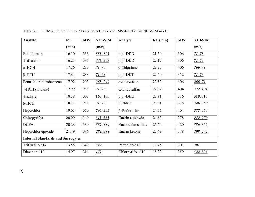
62

Table 3.1. GC/MS retention time (RT) and selected ions for MS detection in NCI-SIM mode.

Analyte RT

(min)

MW NCI-SIM

(m/z)

Analyte RT (min) MW NCI-SIM

(m/z)

Ethalfluralin 16.10 333 333, 303 o,p’-DDD 21.50 306 71, 73

Trifluralin 16.21 335 335, 305 p,p’-DDD 22.17 306 71, 73

-HCH 17.26 288 71, 73 -Chlordane 22.23 406 266, 71

-HCH 17.84 288 71, 73 p,p’-DDT 22.50 352 71, 73

Pentachloronitrobenzene 17.92

293 265, 249 -Chlordane 22.52 406 266, 71

-HCH (lindane) 17.99 288 71, 73 -Endosulfan 22.62 404 372, 404

Triallate 18.38 303 160, 161 p,p’-DDE 22.91 316 318, 316

-HCH 18.71 288 71, 73 Dieldrin 23.31 378 346, 380

Heptachlor 19.63 370 266, 232 -Endosulfan 24.35 404 372, 406

Chlorpyrifos 20.09 349 313, 315 Endrin aldehyde 24.83 378 272, 270

DCPA 20.28 330 332, 330 Endosulfan sulfate 25.64 420 386, 352

Heptachlor epoxide 21.49 386 282, 318 Endrin ketone 27.69 378 308, 272

Internal Standards and Surrogates

Trifluralin-d14 13.58 349 349 Parathion-d10 17.45 301 301

Diazinon-d10 14.97 314 179 Chlorpyrifos-d10 18.22 359 322, 324

62

63

4. RESULTS AND DISCUSSION

In this chapter the occurrence of pesticides studied, and the seasonal and annual

variations of pesticides with high frequency of detection will be discussed. The

relationship of atmospheric concentrations of pesticides with available usage information

and crop production will be discussed. Samples were analyzed by GC/MS in NCI-SIM

mode using an established method [20] that was previously used for analysis of

atmospheric samples collected at Bratt’s Lake, SK in 2003 [6, 19, 73]. A brief overview

of the GC/MS method selection will be provided.

4.1 GC-MS NCI-SIM analysis method

The pesticides selected for this research are GC-amenable and these pesticides are

electrophilic in nature. Pre-emergent herbicides (triallate, trifluralin, ethalfluralin), OP

insecticide (chlorpyrifos), and OC insecticides are all halogenated. A comparison of GC-

MS and GC/MS/MS methods with EI and NCI showed that for the pesticides under study

NCI-SIM mode gave the best overall sensitivity and is less prone to interference issues

[6, 19, 20]. Pesticides in an electron impact source tend to fragment such that the

molecular ion is often not observed. NCI is a softer ionization process than EI so there is

a tendency for less fragmentation, and in a number of cases the quantitative or qualifier

ions (two most abundant ions in the MS spectra) is the molecular ion or a higher mass

product ion as shown in Table 3.1. The presence of higher mass precursor ions or the

molecular ion in NCI improves the potential for lower detection limits as the background

signal is often lower. However for a few pesticides, such as the HCHs, a significant

64

amount of fragmentation in the ion source is still observed, with NCI leading to only a

small mass precursor ion (e.g. m/z=71). In the cases where only one major fragment ion

of sufficient abundance is available for analysis, an isotopic peak (e.g. from 37

Cl) will be

selected for the qualifier ion to confirm the identity of the analyte of interest. This was

the case for HCHs (m/z=71, 73) and chlorpyrifos (m/z=313, 315).

SIM analysis is selected over SRM analysis for the pesticides under study as it

provides better sensitivity. However, NCI-SRM or EI-SIM can be used when added

confirmation is required. In SIM, the quantitative ion is generally the most abundant ion,

while the qualifier is the second most abundant ion with m/z generally selected above 70

to minimize the impact of matrix interferences. Other studies have selected the qualifier

ion as a higher mass fragment ion or the molecular ion (or other isotope peaks

particularly for chlorinated pesticides), however the preference for atmospheric analysis

is to select the two most abundant ions as concentrations analyzed in air extracts are

generally much lower than other matrices such that these alternate ions are too low in

abundance.

65

4.2 Occurrence of pesticides at Bratt’s Lake, SK

Atmospheric sample extracts for samples collected at Bratt’s Lake, SK were

initially analyzed for all the compounds in Table 1.1 which included 12 organochlorine

insecticides, an organophosphorus insecticide (chlorpyrifos), and three pre-emergent

herbicides (triallate, trifluralin, and ethalfluralin). Atmospheric concentrations were

generally below the method detection limit (MDL) for chlordane, DCPA, DDT, DDD,

DDE, endrin aldehyde, (-HCH), heptachlor, and heptachlor epoxide. Due to the low

detection frequency samples collected in 2007-2009 were not analyzed for these

compounds. PCNB was detected in low concentration in 2010 with maximum

atmospheric concentration of 42.7 pg/m3 and concentrations frequently less than 12

pg/m3. Most of the samples analyzed in 2010 during the agricultural season had

concentrations of PCNB <MDL. The atmospheric concentrations of endosulfan sulfate in

2010 were frequently <MDL with only a few periods in summer with concentrations

ranging from 4-83 pg/m3. There was no relationship of endosulfan sulfate with or -

endosulfan and increasing concentrations of endosulfan sulfate during the summer can be

attributed to increased volatilization during warmer summer months.

Atmospheric concentrations of and -endosulfan were much lower than

concentrations of chlorpyrifos and the pre-emergent herbicides. -Endosulfan

concentrations during 2007-2010 reached maximum concentrations from 59-149 pg/m3

(see Table 4.1). The concentrations of -endosulfan during 2007-2010 were significant

higher than in 2003 at Bratt’s Lake, SK when the average concentration of -endosulfan

was 1.77 pg/m3 and maximum concentration was 5.12 pg/m

3 [6]. Endosulfan

concentrations and frequency of detection were lowest in 2009. -Endosulfan

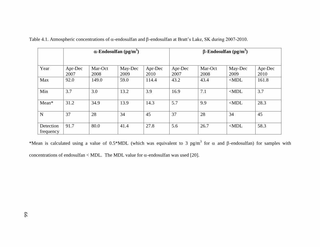
66

Table 4.1. Atmospheric concentrations of -endosulfan and -endosulfan at Bratt’s Lake, SK during 2007-2010.

-Endosulfan (pg/m3) -Endosulfan (pg/m

3)

Year Apr-Dec

2007

Mar-Oct

2008

May-Dec

2009

Apr-Dec

2010

Apr-Dec

2007

Mar-Oct

2008

May-Dec

2009

Apr-Dec

2010

Max

92.0

149.0 59.0 114.4 43.2 43.4 <MDL 161.8

Min

3.7

3.0 13.2 3.9 16.9 7.1 <MDL 3.7

Mean*

31.2 34.9 13.9 14.3 5.7 9.9 <MDL 28.3

N

37 28 34 45 37 28 34 45

Detection

frequency

91.7 80.0 41.4 27.8 5.6 26.7 <MDL 58.3

*Mean is calculated using a value of 0.5*MDL (which was equivalent to 3 pg/m3 for and -endosulfan) for samples with

concentrations of endosulfan < MDL. The MDL value for -endosulfan was used [20].

66

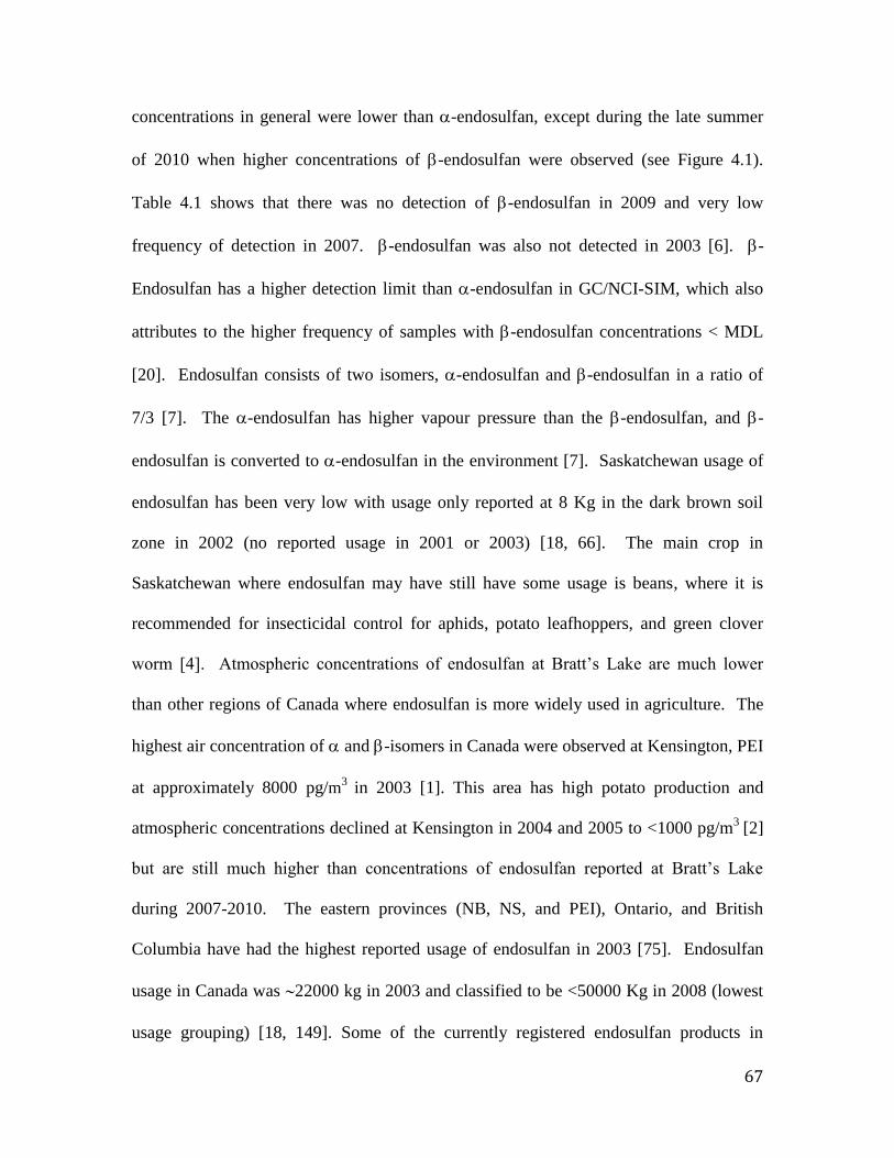
67

concentrations in general were lower than -endosulfan, except during the late summer

of 2010 when higher concentrations of -endosulfan were observed (see Figure 4.1).

Table 4.1 shows that there was no detection of -endosulfan in 2009 and very low

frequency of detection in 2007. -endosulfan was also not detected in 2003 [6]. -

Endosulfan has a higher detection limit than -endosulfan in GC/NCI-SIM, which also

attributes to the higher frequency of samples with -endosulfan concentrations < MDL

[20]. Endosulfan consists of two isomers, -endosulfan and -endosulfan in a ratio of

7/3 [7]. The -endosulfan has higher vapour pressure than the -endosulfan, and -

endosulfan is converted to -endosulfan in the environment [7]. Saskatchewan usage of

endosulfan has been very low with usage only reported at 8 Kg in the dark brown soil

zone in 2002 (no reported usage in 2001 or 2003) [18, 66]. The main crop in

Saskatchewan where endosulfan may have still have some usage is beans, where it is

recommended for insecticidal control for aphids, potato leafhoppers, and green clover

worm [4]. Atmospheric concentrations of endosulfan at Bratt’s Lake are much lower

than other regions of Canada where endosulfan is more widely used in agriculture. The

highest air concentration of and -isomers in Canada were observed at Kensington, PEI

at approximately 8000 pg/m3

in 2003 [1]. This area has high potato production and

atmospheric concentrations declined at Kensington in 2004 and 2005 to <1000 pg/m3

[2]

but are still much higher than concentrations of endosulfan reported at Bratt’s Lake

during 2007-2010. The eastern provinces (NB, NS, and PEI), Ontario, and British

Columbia have had the highest reported usage of endosulfan in 2003 [75]. Endosulfan

usage in Canada was 22000 kg in 2003 and classified to be <50000 Kg in 2008 (lowest

usage grouping) [18, 149]. Some of the currently registered endosulfan products in

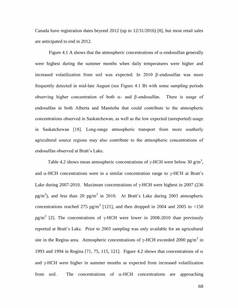
68

Canada have registration dates beyond 2012 (up to 12/31/2016) [8], but most retail sales

are anticipated to end in 2012.

Figure 4.1 A shows that the atmospheric concentrations of -endosulfan generally

were highest during the summer months when daily temperatures were higher and

increased volatilization from soil was expected. In 2010 -endosulfan was more

frequently detected in mid-late August (see Figure 4.1 B) with some sampling periods

observing higher concentration of both - and -endosulfan. There is usage of

endosulfan in both Alberta and Manitoba that could contribute to the atmospheric

concentrations observed in Saskatchewan, as well as the low expected (unreported) usage

in Saskatchewan [18]. Long-range atmospheric transport from more southerly

agricultural source regions may also contribute to the atmospheric concentrations of

endosulfan observed at Bratt’s Lake.

Table 4.2 shows mean atmospheric concentrations of -HCH were below 30 g/m3,

and -HCH concentrations were in a similar concentration range to -HCH at Bratt’s

Lake during 2007-2010. Maximum concentrations of -HCH were highest in 2007 (236

pg/m3), and less than 20 pg/m

3 in 2010. At Bratt’s Lake during 2003 atmospheric

concentrations reached 275 pg/m3 [121], and then dropped in 2004 and 2005 to <150

pg/m3 [2]. The concentrations of -HCH were lower in 2008-2010 than previously

reported at Bratt’s Lake. Prior to 2003 sampling was only available for an agricultural

site in the Regina area. Atmospheric concentrations of -HCH exceeded 2000 pg/m3 in

1993 and 1994 in Regina [71, 75, 115, 121]. Figure 4.2 shows that concentrations of

and -HCH were higher in summer months as expected from increased volatilization

from soil. The concentrations of -HCH concentrations are approaching

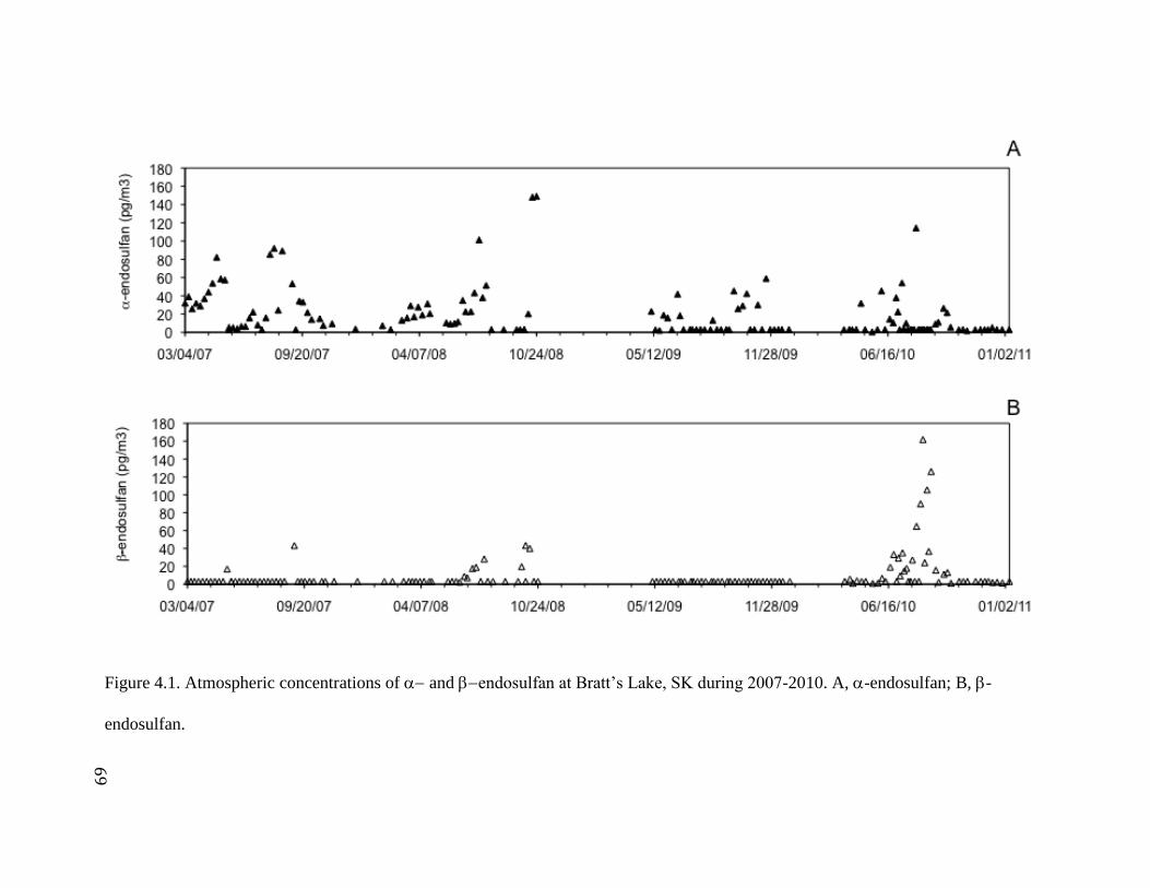
69

Figure 4.1. Atmospheric concentrations of and endosulfan at Bratt’s Lake, SK during 2007-2010. A, -endosulfan; B, -

endosulfan.

69

70

Table 4.2. Atmospheric concentrations of-HCH and -HCH at Bratt’s Lake, SK during 2007-2010.

-HCH (pg/m3)

-HCH (pg/m3)

Year Apr-Dec

2007

Mar-Oct

2008

May-Dec

2009

Apr-Dec

2010

Apr-Dec

2007

Mar-Oct

2008

May-Dec

2009

Apr-Dec

2010

Max

236.2 78.0 48.1 21.3 175.1 102 95.2 19.0

Min

38.7 27.3 13.4 6.1 33.3 25.9 19.6 2.6

Mean

30.8 25.5 12.5 6.1 27.0 23.2 17.0 3.3

25%

Percentile

6.0 13.3 0.5 0.5 0.5 0.5 0.5 0.5

75%

Percentile

41.0 36.9 19.3 8.5 30.3 34.0 22.4 5.5

Median

17.7 22.5 8.5 6.3 12.0 19.1 3.9 1.5

N

37 28 34 45 37 28 34 45

Detection

frequency

83.3 93.3 65.5 88.9 61.1 65.5 69 66.7

70

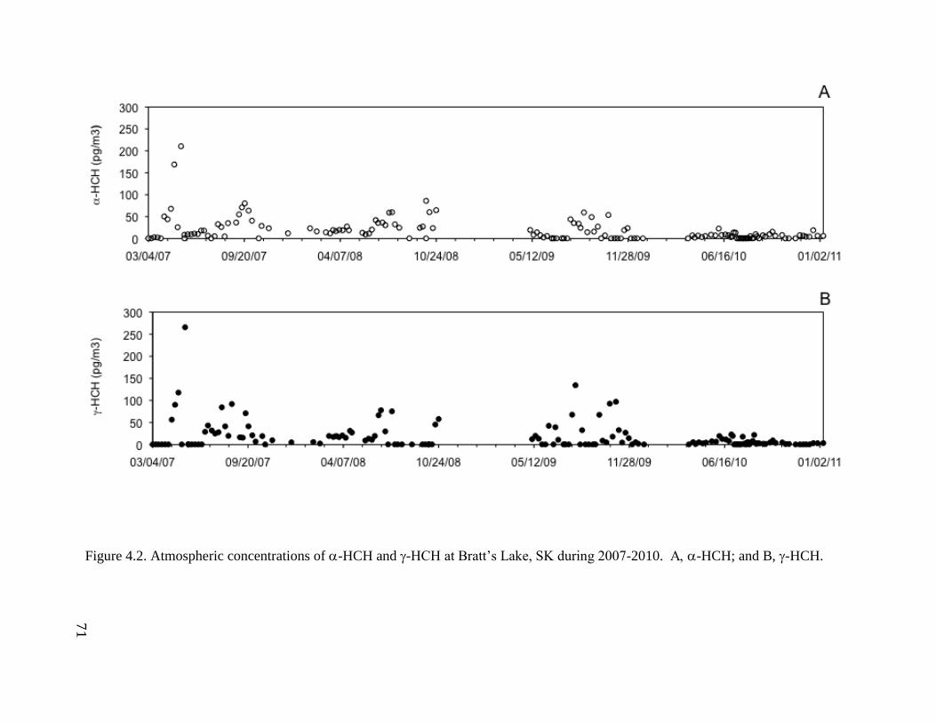
71

Figure 4.2. Atmospheric concentrations of-HCH and -HCH at Bratt’s Lake, SK during 2007-2010.-HCH; and B, -HCH.

71

72

the concentrations of -HCH and Figure 4.2 shows that -HCH concentrations also

increased during the warmer summer months.

Lindane (>90 % -HCH) was widely used in the Canadian prairies and was

registered for use as a seed treatment in Canada in 1951 [73]. Planting of lindane-treated

seeds in the prairies occurred primarily during April and May. The product-life of

lindane products was two years and thus farmers may have used the product into the next

agricultural season after its initial purchase. In 1990, Canada, France, Italy, Niger,

Honduras, the United States, and China were the leading lindane consuming countries

with Canada’s usage in 1980 and 1990 at 286 t/yr and 284.5 t/yr, respectively [74].

Usage of lindane for canola seed treatment in the prairie region in 1997 and 1998 was

estimated at 445.3 and 510.4 t/yr, respectively and the prairies was considered a major

global source region of -HCH [72]. Figure 2.1 A showed that usage in 2001-2003 had

declined from the late 1990s and no usage of lindane was permitted after this time period.

Atmospheric concentrations of -HCH in 2003 still reached 275 pg/m3 and were

influenced by local and regional usage of existing stocks of lindane product. With the

removal from market of lindane products atmospheric concentrations of -HCH have

declined to <20 pg/m3 with similar concentration ranges also reported for -HCH in

2010. These concentrations of and -HCH are considered near background

concentrations for the Pacific Northwest that are influenced by the global atmospheric

distribution of both past usage of lindane and technical HCH [73, 121].

The pesticides with the highest detection frequency at Bratt’s Lake during 2007-

2010 were chlorpyrifos, triallate, trifluralin, and ethafluralin. Comparison of Table 4.3

and 4.4 shows that the highest atmospheric concentrations were observed for chlorpyrifos

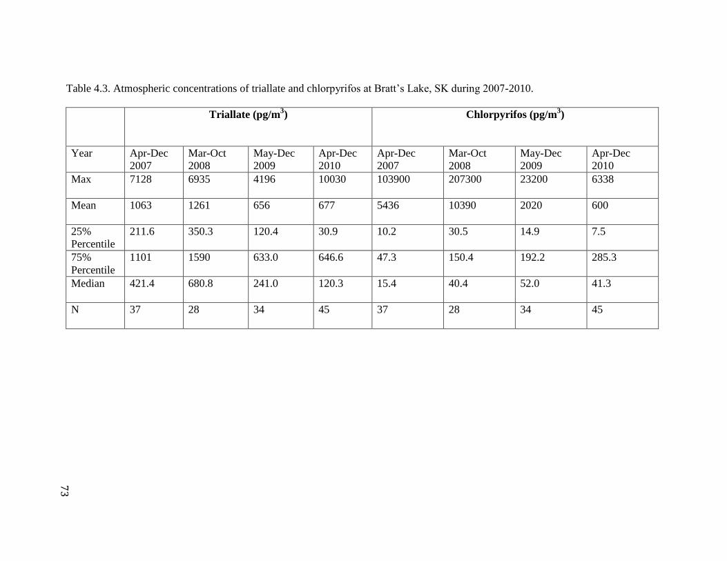
73

Table 4.3. Atmospheric concentrations of triallate and chlorpyrifos at Bratt’s Lake, SK during 2007-2010.

Triallate (pg/m3)

Chlorpyrifos (pg/m3)

Year Apr-Dec

2007

Mar-Oct

2008

May-Dec

2009

Apr-Dec

2010

Apr-Dec

2007

Mar-Oct

2008

May-Dec

2009

Apr-Dec

2010

Max

7128 6935 4196 10030 103900 207300 23200 6338

Mean

1063 1261 656 677 5436 10390 2020 600

25%

Percentile

211.6 350.3 120.4 30.9 10.2 30.5 14.9 7.5

75%

Percentile

1101 1590 633.0 646.6 47.3 150.4 192.2 285.3

Median

421.4 680.8 241.0 120.3 15.4 40.4 52.0 41.3

N

37 28 34 45 37 28 34 45

73

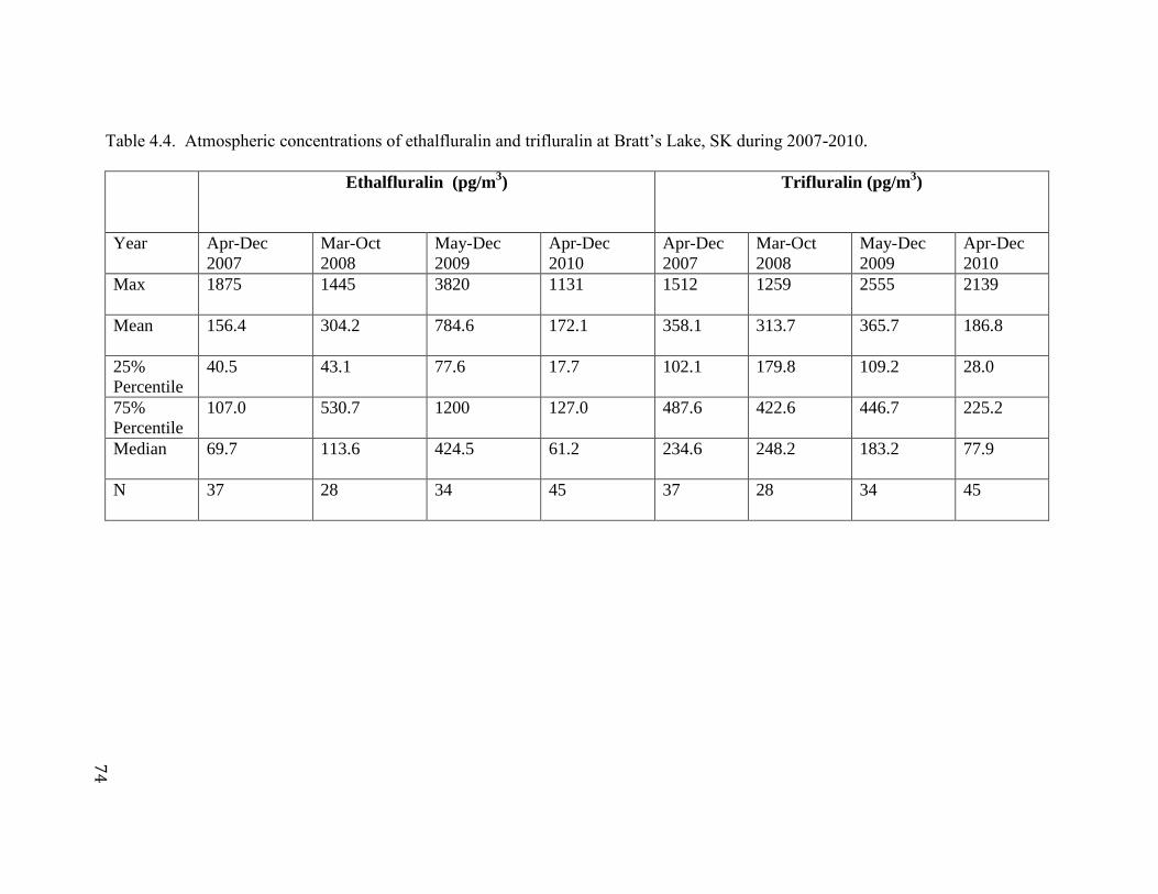
74

Table 4.4. Atmospheric concentrations of ethalfluralin and trifluralin at Bratt’s Lake, SK during 2007-2010.

Ethalfluralin (pg/m3)

Trifluralin (pg/m3)

Year Apr-Dec

2007

Mar-Oct

2008

May-Dec

2009

Apr-Dec

2010

Apr-Dec

2007

Mar-Oct

2008

May-Dec

2009

Apr-Dec

2010

Max

1875 1445 3820 1131 1512 1259 2555 2139

Mean

156.4 304.2 784.6 172.1 358.1 313.7 365.7 186.8

25%

Percentile

40.5 43.1 77.6 17.7 102.1 179.8 109.2 28.0

75%

Percentile

107.0 530.7 1200 127.0 487.6 422.6 446.7 225.2

Median

69.7 113.6 424.5 61.2 234.6 248.2 183.2 77.9

N

37 28 34 45 37 28 34 45

74

75

with mean atmospheric concentration of chlorpyrifos increasing from 2007 to 2008 and

then declining to 2010. The highest atmospheric concentration of chlorpyrifos during

2007-2010 was 207300 pg/m3 and occurred in July 2008. The atmospheric

concentrations of chlorpyrifos observed in 2008 were in a similar concentration range to

those previously observed at Bratt’s Lake in 2003 (maximum of 233000 pg/m3), and

higher than in 2005 (maximum of 1380 pg/m3) [19]. The maximum concentration of

chlorpyrifos in all years from 2007-2010 was higher than that reported in 2005 showing

that the favoured use of this OP insecticide is continuing in the prairie region. As

observed in 2003 and 2005 the mean and maximum concentrations of chlorpyrifos for

each year can vary significantly and it is known from usage data from 2001-2003 that

annual usage of chlorpyrifos can also vary from year to year [5]. The concentrations of

chlorpyrifos were much higher than the concentrations of the pre-emergent herbicides for

2007, 2008, and 2009 (see Table 4.3 and 4.4).

The atmospheric concentrations of triallate were higher in all years (2007-2010)

than concentrations of trifluralin and ethalfluralin (see Table 4.3 and 4.4). Higher

atmospheric concentrations of triallate have been reported at Bratt’s Lake during 1989-

2004 (see Table 2.5) than during 2007-2010, but large annual differences were observed.

The atmospheric concentrations of triallate in 1989 reached 62000 pg/m3

[152], declined

in 2002 to 5460 pg/m3 [142] and then increased in 2003 (>15000 pg/m

3) [1, 6], and then

declined again in 2004 and 2005 (2004, 13000 pg/m3; 2005, 5470 pg/m

3) [2] (see Table

2.5). During these years (1989-2005) the yearly maximum concentrations is >5000

pg/m3 and Table 4.3 shows that the yearly maximum concentration of triallate is >5000

pg/m3 during 2007-2010 except in 2009 (no data available for April). The maximum

76

concentrations observed through 2007-2010 were lower than 1989 and 2003 when the

highest concentrations of triallate were observed at Bratt’s Lake. Canadian usage of

triallate has declined since 2003 with the largest decline in usage of triallate in Alberta

(Canadian usage: 2003, 753500 Kg; 2008, >100000 Kg) [18, 149, 150]. Provincial usage

in Saskatchewan is not available for 2008, however atmospheric concentrations of

triallate at Bratt’s Lake were also much lower in 2008 than 2003. Although usage of

triallate declined in 2008 in Canada, triallate is still the 10th most widely used herbicide

active ingredient. Ethalfluralin usage exceeded triallate usage in 2008 [149], while prior

to this period triallate was more commonly used.

The atmospheric concentrations of trifluralin exceeded 1400 pg/m3 in the Regina

region prior to 1991 (see Table 2.3), however measurements taken at Bratt’s Lake, which

is 35 km southwest of Regina, during 2002 and 2004 showed atmospheric concentrations

of trifluralin <1000 pg/m3. Atmospheric concentrations of trifluralin exceeded 1500

pg/m3 in 2003 and 2005 showing that historically there were large annual changes in

atmospheric concentrations of trifluralin [20]. Table 4.4 shows that in more recent years

maximum concentrations of trifluralin were in the range of 1259 pg/m3 to 2555 pg/m

3

with 2007, 2009, and 2010 observed some sampling periods with triallate >1400 pg/m3 as

had been seen in 2003 and 2005. Mean atmospheric concentrations of trifluralin only

declined in 2010.

Maximum and mean concentrations of ethalfuralin for each year during 2007-

2010 show differences and maximum concentrations were higher than previously

reported at Bratt’s Lake during 2003 and 2004 [1, 2, 6]. During 2007-2010 the highest

atmospheric concentrations of ethalfluralin were reported in 2009 (3820 pg/m3) and

77

Canadian usage of ethalfluralin in 2008 was >500000 Kg as compared to 2003 when

usage was 367000 Kg [5, 18, 121, 149]. Usage in Canada is expected to remain high in

2009 although no usage data is available. The atmospheric concentrations of ethalfluralin

were lower in 2003 (<MDL-620 pg/m3) than during 2007-2010. At Bratt’s Lake higher

atmospheric concentrations of ethalfluralin were also observed in 2005 (7570 pg/m3) [2].

The highest atmospheric concentrations of both ethalfluralin and trifluralin occurred in

2009 even though these two pre-emergent herbicides are supplied in different

formulations. Both ethalfluralin and trifluralin are preferred for use over triallate for

weed control on canola and may be used in combination with other pesticide

formulations [157, 158].

4.3 Atmospheric concentrations of chlorpyrifos and seasonal variation

Figure 4.3 shows that the atmospheric concentrations of chlorpyrifos were low

(frequently <20 pg/m3) but detectable in the winter and spring months, then increased

starting in June, reached peak concentrations during July (chlorpyrifos maximum

concentration: 2007, 103900 pg/m3; 2008, 207342 pg/m

3; 2009, 23200 pg/m

3; 2010, 6338

pg/m3, see Table 4.3). Low concentrations (chlorpyrifos: 2007, <60 pg/m

3; 2008,

~100

pg/m3; 2009, ~80 pg/m

3; 2010, <20 pg/m

3) were also observed in the fall months, when

most insecticide application would have been completed. Previous measurements also

showed the highest concentrations occurred during July (maximum chlorpyrifos 2003,

233000 pg/m3; 2005, 1380 pg/m

3) [19].

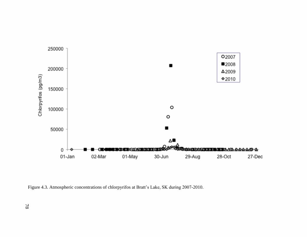
78

Figure 4.3. Atmospheric concentrations of chlorpyrifos at Bratt’s Lake, SK during 2007-2010.

78

79

From the sampling in 2003 and 2005 [19] it was shown that the elevated

concentrations of chlorpyrifos during the summer were due to usage of chlorpyrifos for

grasshopper eradication. There was high usage of chlorpyrifos in 2003 in Canada with

the majority of usage in the prairie provinces [5, 75]. Usage in Alberta and

Saskatchewan was >200,000 kg and significantly greater than in Manitoba [5, 75]. Usage

of chlorpyrifos in Saskatchewan in 2003 was 205,562 Kg relative to in 2001, 2002 when

usage was 2003 of 7267 Kg, and 121,824 Kg, respectively [6]. Usage of chlorpyrifos in

2008 remained >500,000 kg in Canada with the largest usage still expected in

Saskatchewan and Alberta [149]. The higher atmospheric concentrations of chlorpyrifos

observed in 2003 relative to 2005 where attributed to greater usage of chlorpyrifos for

grasshopper infestations in 2003 [19]. However the grasshopper forecast maps for 2007

through 2010 show the lowest densities of grasshoppers in Saskatchewan and the prairies

during 2007 and 2008 (Appendix I) [161]. Atmospheric concentrations of chlorpyrifos

were the highest during summer of 2008 and 2007 when grasshopper counts were low.

Chlorpyrifos is available as an emuslsifiable concentrate (Citadel, Nufos, Lorsban, and

Pyrinex (480 g/L chlorpyrifos)) or as a granular (Pyrifos, 15% chlorpyrifos) [4]. It is also

used for insect control of wheat midge, army cutworms, pale western cutworms, and

bertha armyworms in crops including wheat, barley, oats, canola, flax, and lentils [4].

The wheat midge forecast show high densities of infestations in 2008 and 2007 in the

eastern part of the province more northerly to Bratt’s Lake (Appendix II) [161]. In

addition bertha armyworm forecasts show worsening conditions in 2007 and 2008 when

chlorpyrifos atmospheric concentrations were higher (Appendix III) [161]. Chlorpyrifos

is recommended for control of bertha armyworms on flax and canola [4]. Cabbage

80

seedpod weevil, which can impact quality of canola also showed worsening conditions in

the southwest corner of Saskatchewan during 2008 and 2007, but pyrethroids are

generally applied rather than chlorpyrifos [4]. The higher atmospheric concentrations of

chlorpyrifos in 2008 and 2007 relative to 2009 and 2010 (or 2005 from previous

measurements) are attributed to usage of chlorpyrifos for wheat midge control on wheat

and bertha armyworm control on flax and canola fields. The usage of chlorpyrifos in

Canada remained >500000 kg in 2008 and was a similar magnitude to usage in 2003.

Maximum concentrations of chlorpyrifos in July in 2003 and 2008 were also similar (233

ng/m3 in 2003; 207 ng/m

3 in 2008) [19]. Although in 2007 and 2008 there is more varied

use of chlorpyrifos on different insects, atmospheric concentrations of chlorpyrifos

remained similar in magnitude to that observed in 2003. Chlorpyrifos has also been

detected above 17.5 ng/m3 in 1996 in Sierra Nevada in the Western United States [98].

4.4 Atmospheric seasonal trends in pre-emergent herbicides

Triallate formulations (Avendex Brands or Fortress) are available as an emulsified

concentrate (480 g/L) or granular (10% triallate), or mixed granular (10% triallate and

4% trifluralin) [4]. It can also be used on canola but ethalfluralin and trifluralin are

generally preferred in combination with other pesticides [157, 158]. Triallate is most

commonly used on spring wheat, durum, barley, flax, and mustard [4]. Triallate can be

applied before or after seeding in the spring, or during the fall. The liquid formula is only

recommended for use in the spring, while granulars can be used in spring or fall. Yearly

average atmospheric concentrations of triallate were similar in 2007 and 2008, but were

lower in 2009 and 2010 (see Table 4.3). However, sample analysis in 2009 started in

81

May and given that seeding in 2008 and 2009 were largely completed at the end of May –

beginning of June, atmospheric concentrations of triallate may be above MDL in April

2009 (this data will be added for publication). Atmospheric concentrations in 2010 are

significantly lower than in 2007 or 2008.

Figure 4.4 shows that there is an increase in concentrations of triallate during the

spring to early summer and also an increase in the fall period. These increases in

atmospheric concentration of triallate coincide when usage on crops is recommended.

There are shifts in time of seeding each year due to climatic conditions. In 2010 analysis

of samples taken during April showed much lower concentrations of triallate (see Figure

4.4) than during April 2007 or 2008. The later spring maximum observed for triallate in

2010 relative to 2007 and 2008 is attributed to later seeding of crops. By May 31, 2010

only 59% of crops were seeded relative to 2008 and 2009 when >95% of crops were

planted [162]. In 2007 seeding started at the end of April which is typical for most

years, however there was a small delay of about 1 weeks time compared to other years

such that most of seeding was completed by June 4-10, 2007 [163]. Concentrations of

triallate in 2007 and 2008 during early spring April-May were attributed to recommended

applications of triallate 10-14 days prior to seeding when minimum tillage is used [4]. In

these years seeding generally started by the last week of April. For spring applications

the initial incorporation of granular is completed within 24 hours, while the second

incorporation of granular is delayed a minimum of 48 hours but before crop emergence

such that incorporation can be completed after seeding [4]. During the incorporation

disturbance of surface soils would be expected to increase the potential for volatilization

and consequently higher concentrations of triallate were still

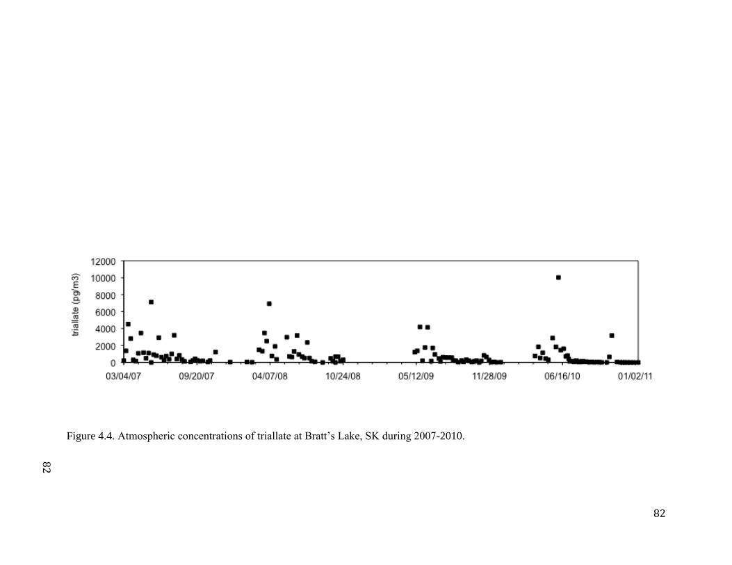
82

Figure 4.4. Atmospheric concentrations of triallate at Bratt’s Lake, SK during 2007-2010.

82

83

observed throughout June and into early July. Temperatures are also higher during these

months which will increase volatilization.

Figure 4.4 shows an increase in concentration of triallate was also observed

during the fall (September and October) in 2007 and 2008, while in 2009 and 2010

increases in concentrations of triallate during the fall occurred only in late October. Fall

applications with conventional tillage are recommended after October 1 but before soil

freeze-up. Fall applications of granular are also made to standing stubble, chemical

fallow, or summerfallow fields when the soil begins to cool (less than 4 C around

October 1) and within 3 weeks of soil freeze-up [4]. Fortress must be applied after

September 15th

and before soil freeze-up. Based on this information application could be

after harvest and in September or after October 1. The time of these increases in

atmospheric concentrations of triallate during 2007-2010 appears to be influenced by

harvest times as well as time of soil freeze-up.

In 2007 and 2008 there were two periods of increases in concentration of triallate

during the fall that occurred in mid September and October coinciding to the two time

periods when applications may occur (after harvest and/or application just prior to soil

freeze-up in early October). The atmospheric concentrations during October could also

be influenced by the second incorporation times for triallate applications that occurred in

September. As in spring the first application is completed within 24 hours, however the

second incorporation of a September application could occur during October prior to soil

freeze-up or in the following spring prior to, or after seeding [4]. In 2007 harvest was

largely completed by October 9th

, with 93% spring wheat, 99% durum, 88% oats, 95%

barely, 86% flax, 92% canola, 99% lentils, and 99% peas [164]. In 2008 harvest was

84

completed around the same time as 2007 (October 5th

) with 97% spring wheat, 96%

durum, 92% oats, 98% barely, 75% flax, 94% canola, 100% lentils, and 99% peas [165].

In 2009 harvest was later with the percentage of crops harvested by October 5th

much

lower. Only 69% spring wheat, 80% durum, 51% oats, 81% barely , 25% flax, 60%

canola, 97% lentils, and 99% peas were harvested by October 5, 2009 [165]. Most of

crop harvesting in 2009 was completed about a week later [166]. In 2010 harvest was

completed even later than in 2009 with 98% spring wheat, 95% durum, 95% oats, 97%

barely, 85% flax, 98% canola, 98% lentils, and 100% peas harvested by October 18, 2010

[167].

Table 4.5 shows that the highest concentrations of triallate during fall were

observed in 2010 with maximum concentration above 3000 pg/m3. In all years the

maximum concentration during the fall occurred after October 1. The higher

concentrations during October 2010 (see Figure 4.5) relative to other years may be

attributed to applications on summerfallow fields for weed control due to high

precipitation amounts in 2010. Saturated soil conditions and continuous rain slowed

seeding and farm operations in 2010. Surplus soil moisture conditions existed in a large

portion of Saskatchewan in 2010 including both high production crop districts 2B and 6A

with many farmers in these regions having some acres of farmland that were flooded and

not suitable for planting. Consequently in these fields where crop was not grown there

were large amounts of weeds present in the fall, and a greater intensity of pre-emergent

herbicides applications were expected during fall 2010 to prepare for the subsequent

agricultural season. Moisture conditions improved in 2011.

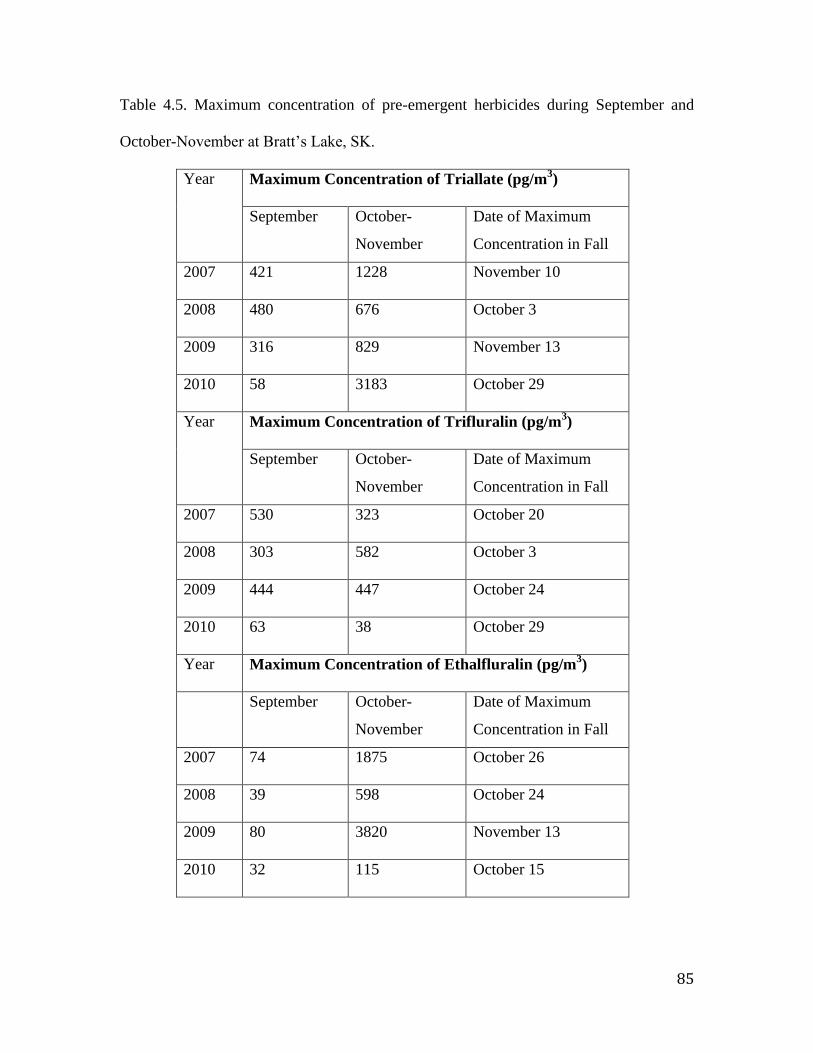
85

Table 4.5. Maximum concentration of pre-emergent herbicides during September and

October-November at Bratt’s Lake, SK.

Year Maximum Concentration of Triallate (pg/m3)

September October-

November

Date of Maximum

Concentration in Fall

2007 421 1228 November 10

2008 480 676 October 3

2009 316 829 November 13

2010 58 3183 October 29

Year Maximum Concentration of Trifluralin (pg/m3)

September October-

November

Date of Maximum

Concentration in Fall

2007 530 323 October 20

2008 303 582 October 3

2009 444 447 October 24

2010 63 38 October 29

Year Maximum Concentration of Ethalfluralin (pg/m3)

September October-

November

Date of Maximum

Concentration in Fall

2007 74 1875 October 26

2008 39 598 October 24

2009 80 3820 November 13

2010 32 115 October 15

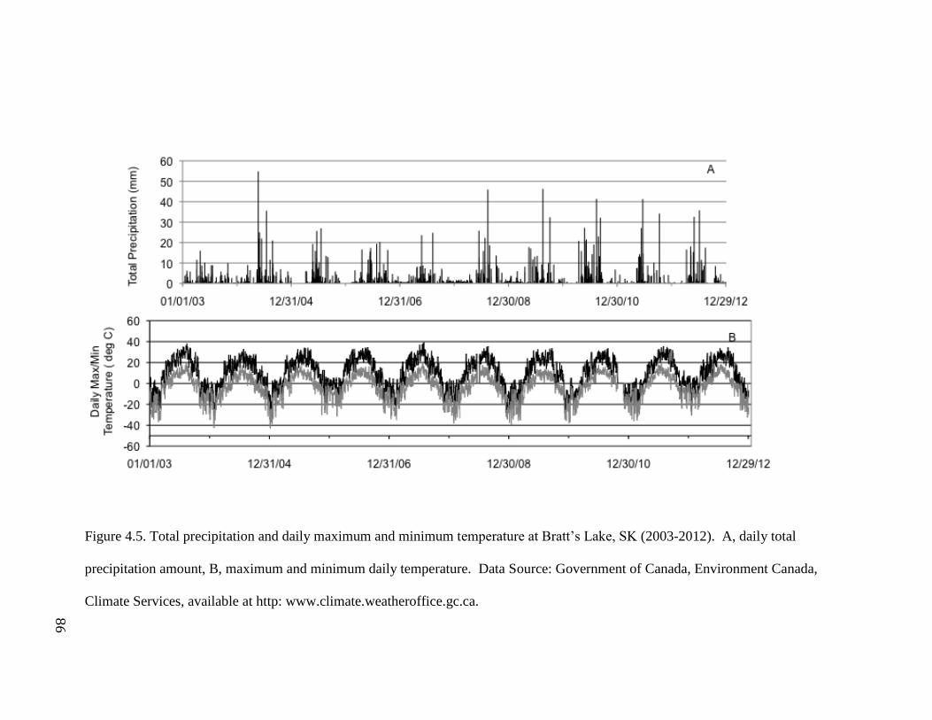
86

Figure 4.5. Total precipitation and daily maximum and minimum temperature at Bratt’s Lake, SK (2003-2012). A, daily total

precipitation amount, B, maximum and minimum daily temperature. Data Source: Government of Canada, Environment Canada,

Climate Services, available at http: www.climate.weatheroffice.gc.ca.

86

87

Figure 4.6 shows that the highest concentrations of trifluralin are observed during

June and July in 2007 and 2008. In 2009 and 2010 concentrations were also high in May

through to the first few weeks of June. In 2009 and 2010 higher concentrations of

triallate were also observed during the same time periods (see Figure 4.4). This suggests

that the formulation more frequently used in 2009 and 2010 was a mixed granular

(Fortress 10% triallate, 4% trifluralin). In 2007 and 2008 there were some periods of

higher concentrations of both trifluralin and triallate, but there were also frequently

periods with only higher concentration of triallate (or trifluralin) particularly in early

spring. This suggests that in these years different formulations of trifluralin were more

commonly in use. In addition to the mixed granular (triallate + trifluralin), trifluralin is

available in an emulsifiable concentrate (480 g L or 500 g L) or a granular with only

trifluralin at 10% [4]. Trifluralin applied as liquid or granular formulations is

recommended on a variety of crops including canola, peas, lentils, barley, flax and wheat

in spring [4], while in the fall only granulars are applied. Trifluralin can be applied from

May through July for weed control during years of fallow-wheat rotation or in the fall

(September or October) or in spring prior to wheat seeding. Liquids are applied in spring

only after seeding (e.g. in June) but prior to crop emergence for crops such as spring

wheat, durum, and barley [4] and are expected to be a major contribution to atmospheric

loadings of trifluralin. Given the half-life of trifluralin and high summer temperatures

increased volatilization of previously applied trifluralin also occurs during the summer.

In addition usage of only granular formulations on summerfallow in the brown soil zone

of Saskatchewan are recommended [4]. The greatest usage of trifluralin (and triallate)

in Saskatchewan occurs in the brown and dark brown soil zones (see Figure 2.1)

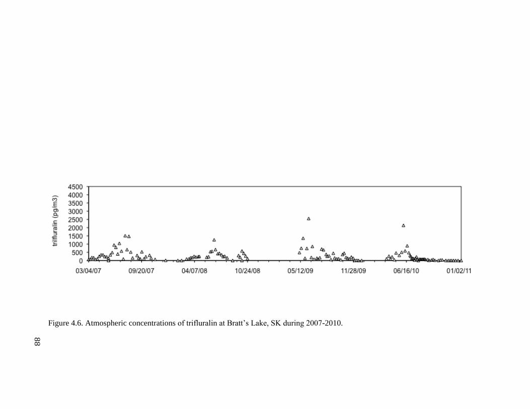
88

Figure 4.6. Atmospheric concentrations of trifluralin at Bratt’s Lake, SK during 2007-2010.

88

89

and the majority of grain and oil seed crops are also grown in the southern portion of the

province such as in crop districts 6A and 2B. Concentrations of trifluralin are relatively

low in the fall compared to triallate and ethalfluralin as shown in Table 4.4. Increase in

fall concentrations of trifluralin occurred in 2007 through 2009 (see Figure 4.6) and may

be partially attributed to favored use of a mixed granular (triallate + trifluralin) or

granular with only trifluralin.

The differences in atmospheric concentrations of trifluralin (and triallate) during

spring are related to shifts in acres of crops harvested during 2007-2010. In

Saskatchewan there was a general increase in canola production from 2003 onward [81].

Crop districts 6A, 6B, and 2B had high acres of canola harvested and crop district 6 B

showed an increase in canola acres harvested from 2007 to 2010 (see Figure 4.7 A).

However in crop district 2B (where Bratt’s Lake is located) canola production decreased

in 2008 and 2009, while in crop district 6A canola acres harvested was lowest in 2010

and 2008. The number of acres of barley harvested in crop district 6A declined from

2007 to 2010 and to a lesser extent in crop district 2B. Most crop districts had a decline

in acres harvested of wheat, durum, and barley in 2010 (see Figure 4.7 A, B, and C).

However, acres of durum harvested in crop district 6B (further north of Bratt’s Lake and

crop district 2B) increased throughout 2007-2010. Flaxseed which also had high

production in crop district 6A and 2B showed declines in acres harvested of flaxseed

from 2008 to 2010, while acres of oats harvested declined in crop districts 2B, 6A and 6B

from 2007 through 2010 (see Figure 4.8 A and B). Specialty crops such as lentils are

one of the few crops that have seen increase in acres harvested from 2007 through 2010

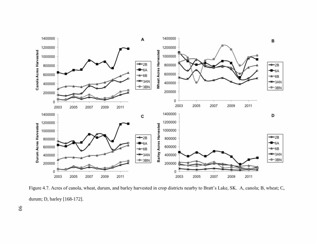
90

Figure 4.7. Acres of canola, wheat, durum, and barley harvested in crop districts nearby to Bratt’s Lake, SK. A, canola; B, wheat; C,

durum; D, barley [168-172].

90

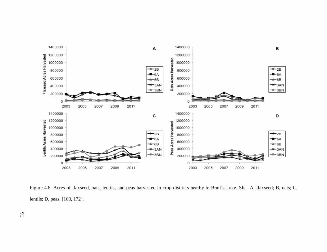
91

Figure 4.8. Acres of flaxseed, oats, lentils, and peas harvested in crop districts nearby to Bratt’s Lake, SK. A, flaxseed; B, oats; C,

lentils; D, peas. [168, 172].

91

92

in many of the crop districts around Bratt’s Lake (crop districts 6A, 6B, 2B, 3AN, 3BN,

see Figure 4.6 C). Acres of peas harvested generally increased from 2007 to 2008, then

decreased as conditions became wetter in 2009 and 2010. Figure 4.5 shows that in 2009

and 2010 a higher frequency of precipitation was observed. The wet conditions lead to

later harvest times in 2009, and later seeding and harvest times in 2010 with decreased

production of most grain crops. The most drastic influence of the wet conditions of 2010

were lower production both locally (crop district 2B) as well as more regionally (crop

district 6A and 6B) for barley, wheat, oats, flaxseed, and peas (see Figure 4.7 and 4.8).

Ethalfluralin is applied as a granular formulation (Edge Granular, 5%) on a

variety of crops including canola, lentils (fall application only), and peas. It is used on

fewer crops than trifluralin and triallate. As observed for other pre-emergent herbicides

an increase in concentration of ethalfluralin is observed during the spring, however spring

concentrations increased from 2007 to 2009, and then during the wet conditions of 2010

decreased again (see Figure 4.9). During the fall increasing concentration of ethalfluralin

was also observed after October. The highest fall concentrations of ethalfluralin were

observed in 2009 which were above 3800 pg/m3 (see Table 4.4). This could be due to

increasing acres of lentils harvested from 2009 to 2010 with recommended fall only

applications of ethalfluralin [4]. In addition, it may have also been used on fields for

weed control due to wetter conditions that started in 2009. Maximum concentration of

both ethalfluralin and triallate occurred on November 13, 2009 (see Table 4.5) suggesting

that some of the usage was related to weed control on fields that were not planted. In fall

2010 the concentrations of ethalfuralin were much lower than in 2009 and acres of lentils

harvested in 2011 also dropped. Ethalfluralin is also more frequently used in the brown

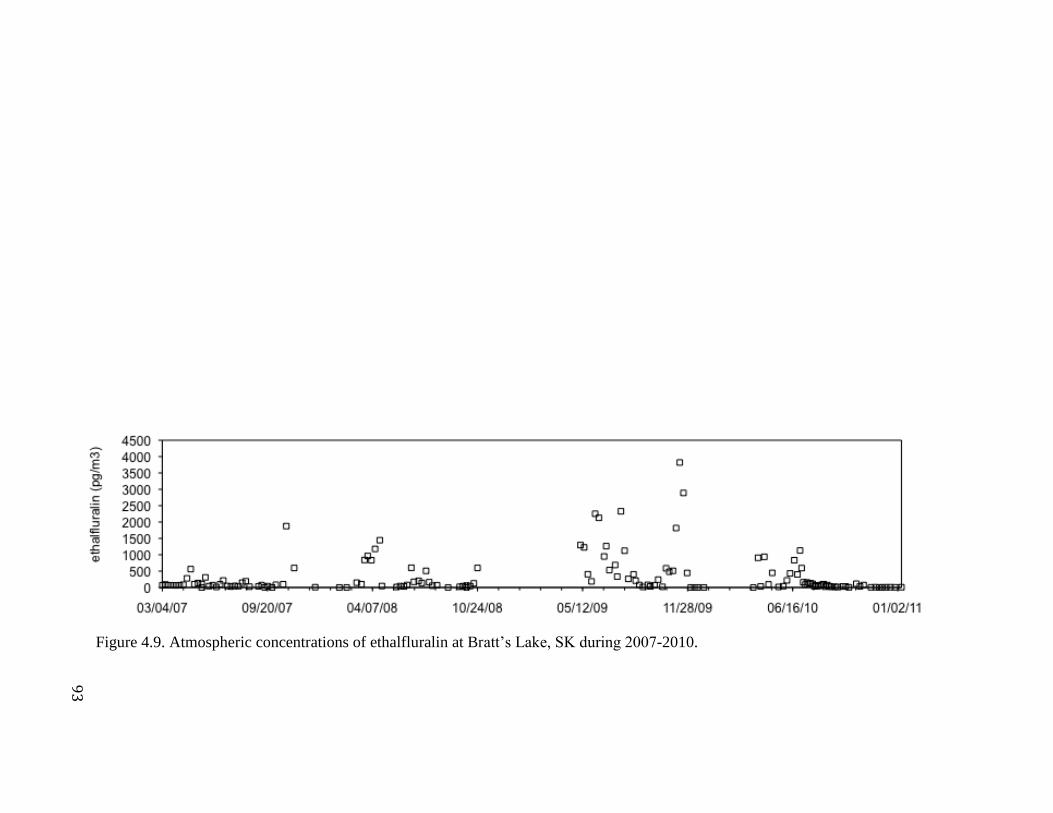
93

Figure 4.9. Atmospheric concentrations of ethalfluralin at Bratt’s Lake, SK during 2007-2010.

93

94

and dark gray soil zones (see Figure 2.1) as compared to triallate and trifluralin which are

used in the brown and dark brown soil zones.

95

5. CONCLUSIONS AND FUTURE WORK

In 2003 and 2005 there was previously air sampling at Bratt’s Lake [19, 20, 74,

81]. This research provides the first long-term trends of selected pre-emergent

herbicides, legacy and current-use organochlorine insecticides (HCHs, endosulfan), and

chlorpyrifos which is a high use organophsophorus insecticide in the prairies. The

sampling years for the research included 2007-2010 and were compared to earlier

measurements at Bratt’s Lake. Samples were analyzed by GC/MS, using a developing

method for analysis of pesticide residues in air extracts [20].

5.1 Air concentrations of pesticides

In 2007-2010 maximum concentrations of chlorpyrifos were observed during July

which was previously reported in 2003 and 2005 [19]. Maximum concentrations of

chlorpyrifos occurred in July 2008 (207300 pg/m3) and were similar to the maximum

observed in 2003 (233000 pg/m3) [19]. The high concentrations of chlorpyrifos in 2008

were attributed to high usage (e.g. Canada >500000 Kg) for insect control for wheat

midge and bertha armyworm. This differed from 2003 when the high atmospheric

concentrations of chlorpyrifos were due to high usage for grasshopper eradication.

Higher atmospheric concentrations of chlorpyrifos can be associated to years when there

are greater insect counts and demand for usage of chlorpyrifos.

Maximum concentrations of triallate (10030 pg/m3) were higher than trifluralin

(2555 pg/m3) and ethalfluralin (3820 pg/m

3) in 2007-2010, but lower than chlorpyrifos.

Usage of triallate in Canada has declined since 2003; however atmospheric

96

concentrations of triallate during 2007-2010 remain similar to the previous

measurements. Maximum concentrations of pre-emergent herbicides were observed

during spring-early summer when they are recommended to be applied for weed control.

Atmospheric concentrations may increase during the fall as associated with applications

after harvest in September or after October 1 prior to soil freeze-up. The time period of

higher concentrations of pre-emergent herbicides shifted with seeding time and harvest

times (freeze-up). In 2003 Alberta had much higher usage than Saskatchewan [18], and

usage in 2008 in Alberta declined [150].

Atmospheric concentrations of trifluralin exceeded 1500 pg/m3 in 2003 and 2005

as compared to the previous measurement in 1991 (maximum ranging from 1400-3600

pg/m3

in Regina area). In more recent years (2007-2010) maximum concentrations of

trifluralin were in the range of 1259 pg/m3 to 2555 pg/m

3 showing that trifluralin is still

heavily used in the region.

Historically atmospheric concentrations of ethalfluralin have shown large annual

variations in concentration range. The atmospheric concentrations of ethalfluralin were

<MDL-620 pg/m3 in 2003, while 762-7570 pg/m

3 in 2005. During 2007-2010 the highest

atmospheric concentrations of ethalfluralin occurred in 2009 (3820 pg/m3). Both

ethalfluralin and trifluralin are preferred for use over triallate for weed control on canola

and canola production has increased in the prairies. Ethalfluralin is also used for weed

control for lentils and may be applied in fall. Production of lentils also increased in

Saskatchewan. Both trifluralin and ethalfluralin formulations may be used in

combination with other pesticide formulations to minimize crop resistance.

In general 2010 showed the lowest concentrations of the pre-emergent herbicides

97

(as well as chlorpyrifos). The lower atmospheric concentration of these pesticides are

attributed to a decrease in grain crop production as a result of high precipitation

occurrence and flooding conditions on farms in the prairies. The highest fall

concentrations of triallate were observed in 2010 as expected to be due to preferred usage

of granular (triallate or triallate+ethalfluralin combination) for weed control on fields that

were not planted in preparation for the next agricultural season. Wet conditions started in

the fall of 2009 as noted by the late harvest in 2009. During the fall of 2009 ethalfluralin

concentrations were the highest and may be attributed to usage for weed control on

dormant fields as well as crops such as lentils which had higher production.

These three pre-emergent herbicides are among the most frequently detected

pesticides at Bratt’s Lake and atmospheric concentrations are at levels of concern for

long-range atmospheric transport to sensitive areas such as the Arctic. Based on the

atmospheric concentrations of pre-emergent herbicides observed, the Canadian prairies

would be considered a major global source region. Trifluralin is currently under

evaluation as a potential POPs to be added to the Stockholm Convention. The data

presented in this thesis will be supportive to addition of trifluralin to the POPs list and

also consideration of the other two pre-emergent herbicides to the Stockholm convention

or future restrictions in usage in Canada. The pre-emergent herbicides have similar

volatility and half-life and with increasing canola production in the prairies trifluralin and

ethalfluralin usage is expected to remain high.

Concentrations of -HCH have declined from 175 pg/m3

in 2007 to 19 pg/m3

reported in 2010 with the elimination of usage of lindane for seed treatment in the

prairies in 2003. Endosulfan concentrations are low at Bratt’s Lake and current usage in

98

Saskatchewan is expected to be low. Future measurements with restrictions anticipated

on endosulfan usage starting in 2012 may result in further declines in atmospheric

concentrations of endosulfan. As of April 2013 there are still 5 endosulfan products

registered for use in Canada with expiration dates of registrations up to December 31,

2016. The data from 2007-2010 at Bratt’s Lake will be valuable as a background site for

comparison to global atmospheric concentrations of endosulfan with Bratt’s Lake site

identified as a site with little to no local usage.

5.2 Future work

Chlorpyrifos usage remained high in Canada in 2008. Atmospheric concentrations

of chlorpyrifos were also high for the years with larger densities of infestations of wheat

midge and bertha armyworms. Future analysis should include examination of the

concentrations of chlorpyrifos oxon by LC/MS/MS particularly in 2007 and 2008 when

atmospheric concentrations of chlorpyrifos were high. Determining the concentration of

the degradation product of chlorpyrifos in the atmosphere with provide an indication of

the age of the formulation, and help to determine the extent of regional versus local

atmospheric transport. Based on insect forecast maps for wheat midge and bertha

armyworms it is anticipated that regional atmospheric transport from more northerly high

production crop districts (e.g. crop district 6A) to Bratt’s Lake will be most important.

This project can be expanded for monitoring malathion or diazinon due to recommended

usage now extending to a wide range of crops for insect control of aphids, grasshoppers,

and leafhopper. In prior measurements in 2003 and 2005 atmospheric concentrations of

malathion were much lower than chlorpyrifos, but with its wider potential usage

99

including on canola atmospheric concentrations of malathion may have increased.

The atmospheric concentrations of the pre-emergent herbicides remained high

enough to be of concern in 2007-2010 at Bratt’s Lake. Future studies examining the

potential for regional to long-range atmospheric transport should be continued. This may

include additional sampling sites such as in North Dakota (source region south of

Saskatchewan for trans-boundary atmospheric transport) and potentially sites in crop

districts 6A, 6B, 3AN, and 3BN to allow better assessment of regional inputs. With this

new sampling, stronger relationships of atmospheric concentrations of pre-emergent

herbicides with acres of crops harvested or crop productions could be investigated.

100

REFERENCE

[1] Yao, Y.; Tuduri, L.; Harner, T.; Blanchard, P.; Waite, P.; Poissant, L.; Murphy,

C.;Belzer, W.; Aulagnier, F.; Li, Y.-f.; Sverko, E. Atmos. Environ. 2006, 40, 4339-4351.

[2] Yao, Y.; Harner, T.; Blanchard, P.; Tuduri, L.; Waite, D.; Poissant, L.; Aulagnier,

F.;Sverko, E. Environ. Sci. Technol. 2008, 42, 5931-5937.

[3] Kang, J.-H.; Chang, Y.-S. Chapter 9, Organochlorine Pesticides in Human Serum.

Pesticides-Strategies for Pesticides Analysis, Stoytcheva, M, Intech, 2011, Rijeka, Crotia

ISBN: 978-953-307-406-3.

[4] Government of Saskatchewan: Ministry of Agriculture, 2010 Guide to Crop

Protection, Regina, 2012.

[5] Saskatchewan Usage Inventory 2003, Personnel Communication, Saskatchewan

Agriculture, 2003.

[6] Hall, P. GC/MS and GC/MS/MS Analysis and Atmospheric Concentrations

Organochlorine and Organophosphorus Pesticides and Selected Current Us Herbicides in

Saskatchewan. Ph D Thesis, University of Regina. 2010.

[7] Tuduri, L.; Harner, T.; Blanchard, P.; Li, Y.-F.; Poissant, L.; Waite, D.T.; Murphy,

C.;Belzer, W. Atmos. Environ. 2006, 40, 1563-1578.

[8] Consumer Product Safety, Pesticides & Pest Management, Registrants & Applicants

Health Canada, 2012, http://www.hc-sc.gc.ca/cps-spc/pest/registrant-titulaire/index-

eng.php.

[9] Stockholm Convention on Persistent Organic Pollutants (POPs), 2011,

http://www.environment.gov.au/settlements/chemicals/international/index.html.

[10] Li, Y.F.; Bidleman, T.F.; Barrie, L.A. Geophys. Res. Lett. 1998, 25, 39-41.

101

[11] Bailey, R.; Barrie, L.A.; Halsall, C.J.; Fellin, P.; Muir, D.C.G. J. Geophys. Res.

2000, 105, 11,805- 11,811.

[12] Hung, H.; Halsall, C.J.; Blanchard, P.; Li, H.H.; Fellin, P.; Stern, G.; Rosenberg, B.

Environ. Sci. Technol. 2002, 36, 862-868.

[13] Voldner, E.C.; Li, Y.-F. Sci. Total Environ.1995, 160/161, 201-210.

[14] Bierman, V.; Swain, W. Environ. Sci. Technol. 1982, 16, 572-579.

[15] Geyer, H.J.; Rimkus, G.C.; Scheunert, I.; Kaune, A.; Schramm, K.-W.; Kettrup, A.;

Zeeman, M.; Muir, D.C.G.; Hansen, L.C.; Mackay, D. Chemosphere. 2000, 13, 269-284.

[16] Lundholm, C.E. Comp. Biol. Physiol. 1997, 118, 113-128.

[17] Lopez, J.; Catala-Icardo, M. Anal. Lett. 2011, 44, 146-175.

[18] Brimble, S.; Bacchus, P.; Caux, P.-Y. Pesticide Utilization in Canada: A

Compilation of Current Sales and Use Data; Environment Canada, 2005, Gatineau, QC.

[19] Raina, R.; Hall, P.; Sun, L. Environ. Sci. Technol. 2010, 44, 8541-8546.

[20] Raina, R.; Hall, P. Analytical Chemistry Insights. 2008, 3, 111–125.

[21] Aguilar, A.; Borrell, A. Marine. Environ. Res. 2005, 59, 391-404.

[22] Fitzgerald, E.; Hwang, S.A.; Deres, D.A.; Bush, B.; Cook, K.; Worswick, P. J.

Exposure. Anal. Environ. Epidemiol, 2001, 11, 381–388.

[23] Kamel, F.; Hoppin, J. Environ. Health Perspect. 2004, 112, 950-958.

[24] Mathur, V.; Bhatnagar, P.; Sharma, R.G.; Acharya, V.; Sexana, R. Environment

International. 2002, 28, 331-336.

[25] Solomon, G.M.; Weiss, P.M. Environ. Health Perspect. 2002, 110, 339-347.

[26] Matthew, P.; Longnecker, MD.; Klebanoff, M.A.; Haibo Zhou, MD.; Brock, J.W.

The Lancet. 2001, 358, 110-114.

102

[27] MacDonald, R.W.; Barrie, A.L.; Bidleman, T.F.; Diamond, M.L.; Gregor, D.J.;

Semkin, R.J.; Strachan, W.M.J.; Li, Y.F.; Wania, F.; Alaee, M.; Alexeeva, L.B.;

Backus, S.M.; Bailey, R.; Bewers, J.M.; Gobeil, C.; Halsall, CG.; Harner, T.;Hoff, J.T.;

Jantunen, L.M.M.; Lockhart, W.L.; MacKay, D.; Muir, D.C.G.; Pudykiewicz, J.; Reimer,

K.J.; Smith, J.N.; Stern, G.A.; Schroeder, W.H.; Wagemann, R.; Yunker, M.B. Sci. Total

Environ. 2000, 245, 93-110.

[28] Norheim, G.; Utne Skaare, J.; Wiig, Q. J. Environ. Pollut. 1992, 77, 51-57.

[29] Hoferkamp, L.; Hermanson, M.H.; Muir, D.C.G. Sci. Total. Environ. 2010, 408,

2985-2994.

[30] Letcher, R.J.; Bustnes, J.O.; Dietz, R. Sci. Total. Environ. 2010, 408, 2995–3002.

[31] Weber, J.; Halsall, C.J.; Muir, D.; Teixeira, C.; Small, J.; Solomon, K.; Hermanson,

M.; Hung, H.; Bidleman, T. Sci. Total. Environ. 2010, 408, 2966–2984.

[32] Medehouenou, T.C.M.; Ayotte, P.; Carmichael, P.H.; Kroger, E.; Verreault, R.;

Lindsay, J.; Dewailly, E.; Tyas, S.L.; Bureau, A.; Laurin, D. Environmental Research.

2011, 111, 1313-1320.

[33] Eskenazi, B.; Bradman, A.; Castorina, R. Environ. Health Perspect. 1999, 107, 409-

419.

[34] Koureas, M.; Tsakalof, A.; Tsatsakis, A.; Hadjichristodoulou, C. Toxicology Letters,

2012, 210, 15-168.

[35] Bhat, A.R.; Wani, M.A.; Kirmani, A.R.; Raina, T.H. Indian. J. Med. Paediatr.

Oncol. 2010, 31.

103

[36] Sun, L. Determination of Organophosphorus Pesticides and their Degradation

Products in Atmospheric Samples in Western Canada by LC/ESI+-MS/MS. M Sc

Thesis, University of Regina. 2009.

[37] Matsumura, F.; Krishna Murti, C.R. Biodegradation of Pesticides. Plenum Press,

New York, 1982.

[38] Pope, C.N. J. Toxicol. Environ. Health. B. 1999, 2, 161-181.

[39] Colborn, T.; Short, P. J. Toxicol. Ind. Health. 1999, 15, 241–276.

[40] Ribas, G.; Surrallrs, J.; Carbonell, E. Mutation Res. 1996, 371, 15–21.

[41] Ribas, G.; Frenzilli, G.; Barale, R.; Marcos, R. Mutation Res. 1995, 344, 41–54.

[42] Semchuk, K.M.; McDuffie, H.H.; Senthilselvan, A.; Cessna, A.J.; Irvine, D.G. J.

Toxicol. Environ. Health. A. 2004, 67, 1341–1352.

[43] Kreuzig, R. International HCH and Halogenated Pesticides Forum, Compilation

1stand 2

nd HCH-Forum. 1994, 114–121.

[44] Zhang, G.; Li, J.; Cheng, H.R.; Li, X.D.; Xu, W.H.; Jones, K.C. Environmental

Science and Technology, 2007, 41, 3884-3890.

[45] Hartley, D.; Kidd, H. (Editors), The Agrochemicals Handbook. 2nd Ed., The Royal

Society of Chemistry, London, UK, 1987.

[46] Tomlin, C. The Pesticide Manual (A World Compendium). 10th Ed., Incorporating

the Agrochemicals Handbook.; The British Crop Protection Council: Surrey, UK, The

Royal Society of Chemistry, Cambridge, UK, 1994.

[47] Material Safety Data Sheet, Chem Service Inc., West Chester, PA, USA (2010).

[48] Hornsby, A.G.; Wauchope, R.D.; Herner, A.E. Pesticide Properties in the

Environment. Springer-Verlag Inc., New York, 1996.

104

[49] Wauchope, R.D.; Buttler, T.M.; Hornsby A.G.; Augustijn Beckers, P.W.M.; Burt, J.

P. Rev. Environ. Contam. Toxicol. 1992, 123: 1-157.

[50] Parr, J.; Smith, S. Soil Sci. 1973, 115, 55.

[51] Agriculture and Environmental Research Unit (AERU), University of Hertfordshire,

UK, Pesticide Properties Database (PPDB), available at

http://sitem.herts.ac.uk/AERU/projects/ppdb/index.html.

[52] Weed Science Society of America. Herbicide Handbook, Seventh Edition.

Champaign, IL, 1994, editor Ahrens, W.H.

[53] Health and Ecological Criteria Division Office of Science and Technology, Office of

Water. U.S. Environmental Protection Agency. Washington, DC 20460, Drinking Water

Health Advisory for Dacthal and Dacthal Degradates: Tetrachloroterephthalic Acid

(TPA) and Monomethyl Tetrachloroterephthalic Acid (MTP). Document Number: 822-

R-80-011. 2008.

[54] Hinckley, D.A.; Bidleman, T.F.; Foreman, W.T. J. Chem. Eng. Data. 1990, 35, 232-

237.

[55] Mabey, W.R.; Smith, J.H.; Podoll, R.T.; Johnson, H.L.; Mill, T.; Chou, T.-W.;

Gates, J.; Partridge, I.W.; Jaber, H.; Vandenberg, D. Aquatic Fate Process Data for

Organic Priority Pollutants. Washington, D.C., U.S. Environmental Protection Agency

(EPA), 1982, 440, 4-81.

[56] Shiu, W.Y.; Ma, K.C.; Mackay, D.M.; Seiber, J.N.; Wauchope, R.D. Reviews of

Environmental Contamination and Toxicology. 1990, 116, 15-187.

[57] Meijer, S.N.; Halsall, C.J.; Harner, T.; Peters, A.J.; Ockenden, W.A.; Johnston, A.E.;

Jones, K.C. Environ. Sci. Technol, 2001, 35, 1989-1995.

105

[58] Kanazawa, J.; Yushima, T.; Kiritani, K. Kagaku. 1971, 41(7), 384-391.

[59] Majewski, M.S.; Capel, P.D. Pesticides in the Atmosphere. Distribution, Trends,

and Governing Factors. Vol. 1 of the Series Pesticides in the Hydrologic System. Ann

Arbor Press, Chelsea, MI., 1995.

[60] Slade, R.E. Chem. Ind. 1945, 40, 314-319.

[61] Unsoworth, J.B.; Wauchope, R.D.; Klein, A.W.; Dorn, E.; Zeeh, B.; Yeh, S.M.;

Akerblom, M.; Racke, K.D.; Rubin, B. Pure Appl. Chem. 1999, 71, 1359-1383.

[62] Augustijn-Beckers, P.W. M., Hornsby, A.G.; Wauchope, R.D. Rev. Environ.

Contam. Toxicol. 1994, 137, 1-82.

[63] U.S. Department of Health and Human Services. Hazardous Substances Data Bank

(HSDB, online database). National Toxicology Information Program, National Library of

Medicine, Bethesda, MD. 1993.

[64] Howard, P.H., Ed. Handbook of Environmental Fate and Exposure Data for Organic

Chemicals. Vol 3: Pesticides. Lewis Publishers, Chelsea, MI, 1991, 5-13

[65] Halfon, E.; Galassi, S.; Bruggemann, R.; Provini, A. Chemosphere, 33, 1996, 1543.

[66] Pait, A.S.; De Souza, A.E.; Farrow, D. R. G. United States. National Ocean Service.

Strategic Environmental Assessments Division, Agricultural pesticide use in coastal

areas: a national summary. Strategic Environmental Assessments Division, Office of

Ocean Resources Conservation and Assessment, National Ocean Service, National

Oceanic and Atmospheric Administration, Rockville, Md., 1992, 112.

[67] Kubiak, R.; Burkle, L.; Cousins, I.; Hourdakis, A.; Jarvis, T.; Jene, B.; Koch, W.;

Kreuger, J.; Maier, W.; Millet, M.; Reinert, W.; Sweeney, P.; Tournay, J.; Van den Berg,

F. Pesticides in Air: Consideration for Exposure Assessment. Report of the FOCUS

106

Working Group on Pesticides in Air, EC Document Reference SANCO/10553/2006 Rev

2, 2008.

[68] Raina, R.; Belzer, W.; Jones, K. Air, Soil and Water Rec. 2009, 2, 41-49.

[69] Barrett, K.; Jaward, F.M. International Journal of Environmental Health Research.

2012, 1-19.

[70] Raina, R.; Etter, M.L. Anal. Chem. Insights 5, 2010, 1-15.

[71] Waite, D.T.; Cessna, A.J.; Gurprasad, N.P.; Banner, J. Atmos. Environ. 1999, 33

1513-1523

[72] Waite, D.T.; Gurprasad, N.P.; Sproull, J.F.; Quiring, D.V.; Kotylak, M.W. Environ,

J. Qual., 2001, 30, 768-775.

[73] Raina, R.; Hall, P. Air, Soil, and Water Research, 2010, 3, 57-66.

[74] Skoog, D.A.; Holler, F. J.; Nieman, T.A. Principles of Instrumental Analysis, 5th

ed.;

Harcourt Brace: Toronto, 1998.

[75] Brimble, S. Pesticide Utilization in Canada: A Compilation of Current Sales and Use

Data. Environment Canada, Ottawa, 2003.

[76] McNair, H.M.; Miller, J.M. Basic Gas Chromatography; Wiley: Toronto, 1998.

[77] Garrido Frenich, A.; Plaza-Bolanos, P.; Martinez Vidal, J.L. J. Chromatogr, A.

2008, 1203, 229-238.

[78] Nevado, J.J.B.; Martin-Doimeadios, R.C.R.; Bernardo, F.J.G.; Farinas, N.R.;

Cogolludo, J.M.G.; Osma, J.A.C. Talanta. 2010, 81, 887-893.

[79] Borras, E.; Sanchez, P.; Munoz, A.; Tortajada-Genaro, L.A. Anal. Chem. Acta. 2011,

699, 57-65.

[80] Elflein, L.; Berger-Preiss, E.; Levsen, K.; Wu¨nsch, G. J. Chromatogr, A. 2003, 985,

107

147-157.

[81] Raina, R. Pesticides, Chapter 5, Chemical Analysis of Pesticides using GC/MS,

GC/MS/MS, Pesticides-Strategies for Pesticides Analysis, Stoytcheva, M, Intech, 2011,

Rijeka, Crotia, ISBN: 978-953-307-406-3.

[82] Huskova, R.; Matisova, E.; Svorc, L.; Mocak, J.; Kirchner, M. J. Chromatogr, A.

2009, 1216, 4927-4932.

[83] Huskova, R.; Matisova, E.; Hrouzkova, S.; Svorc, L. J. Chromatogr, A. 2009, 1216,

6326-6334.

[84] Ricardo Rodrı´guez, L.B.; Ricardo Rodrı´guez, E.; Ellington, J.J.; Evans, J.J.

Environmental Pollution. 2007, 148, 654-662.

[85] Amendola, L.; Botrè, F.; Carollo, A.S.; Longo, D.; Zoccolillo, L. Anal. Chem. Acta.

2002, 461, 97-108.

[86] Hoffmann, E.; Stroobant, V. Mass Spectrometry: Principles and Applications, 3th

ed.; Wiley: Toronto, 2007.

[87] Yoshida, T.; Matsunaga, I.; Oda, H. J. Chrom. A. 2004, 1023, 255.

[88] Albanis, T.A.; Hela, D.G. J. Chrom. A. 1995, 707, 283.

[89] Tagami, T.; Kagimura, K.; Takagi, S. Pharmaceutical Society of Japan. 2007, 127

(7) 1167-1171.

[90] Mario, V.R.; Campanella, L.; Avino, P. J. Chromatogr, B. 2002, 780, 431-441.

[91] Mart´ınez Vidal, J.L.; Arrebola, F.J.; Mateu-Sa´nchez, M. J. Chromatogr, A. 2002,

959, 203-213.

[92] Walorczyk, S. J. Chromatogr, A. 2008, 1208, 202-214.

[93] Li, Y.-F.; Macdonald, RW. Sci. Total Environ. 2005, 342, 87-206.

108

[94] USEPA, Endosulfan: Final Product Cancellation Order.,Washington, DC., 2010, Pg

69065-69069.

[95] Harner, T.; Shoeib, M.; Kozma, M.; Gobas, F.; Li, S.M. Environ. Sci. Technol. 2005,

39, 724-731.

[96] Moreau-Guigon, E.; Motelay-Massei, A.; Harner, T.; Pozo, K.; Diamond, M.;

Chevreuil, M.; Blanchoud, H. Environ. Sci. Technol. 2007, 41, 2172-2177.

[97] Hoh, E.; Hites, R.A. Environ. Sci. Technol. 2004, 38, 4187-4194.

[98] Lenoir, J.S.; McConnell, L.L.; Fellers, G.M.; Cahill, T.M.; Seiber, J.N. Environ.

Toxicol. Chem. 1999, 18, 2715-2722.

[99] Pozo, K.; Harner, T.; Lee, S.C.; Wania, F.; Muir.; D.C.G.; Jones, K.C. Environ. Sci.

Technol. 2009, 43, 796-803.

[100] Harman-Fetcho, J.A.; Mcconnell, L.L.; Rice, C.P.; Baker, J.E. Environ. Sci.

Technol. 2000, 34, 1462-1468.

[101] Wong, F.; Alegria, H.A.; Bidleman, T.F.; Alvarado, V.; Angeles, F.; A´vila

Galarza, A.; Bandala, E.R.; de la Cerda Hinojosa, I.; Galindo Estrada, I.; Galindo Reyes,

G.; Gold-Bouchot, G.; Vinicio Macı´as Zamora, J.; Murguı´a-Gonza´ lez, J.; Ramirez

Espinoza, E. Environ. Sci. Technol. 2009, 43, 704-710.

[102] Wong, F.; Alegria, H.A.; Bidleman, T.F. Environ. Pollut. 2010, 158, 749–755.

[103] Estellano, V.R.H.; Pozo, K.; Harner, T.; Franken, M.; Zaballa, M. Environ. Sci.

Technol. 2008, 42, 2528-2534.

[104] Meire, R.O.; Lee, S.C.; Yao, Y.; Targino, A.C.; Torres, J.P.M.; Harner, T. Atmos.

Environ. 2012, 59, 108-116.

[105] Chakraborty, P.; Zhang, G.; Li, Y.; Xu, Y.; Liu, X.; Tanabe, S.; Jones, K.C.

109

Environ. Sci. Technol. 2010, 44, 8038–8043.

[106] Karlsson, H.; Muir, D.C.G.; Teixiera, C.F.; Burniston, D.A.; Strachan, W.M.J.

Hecky, R.E.; Mwita, A.; Bootsma, H.A.; Grift, N.P.; Kidd, K.A.; Rosenberg, B. Environ.

Sci. Technol. 2000, 34, 4490-4495.

[107] Health Canada, Consumer Product Safety, Product Label Search, accessed 2013,

available at http://pr-rp.hc-sc.gc.ca/ls-re/index-eng.php.

[108] Saskatchewan Agriculture, Food and Rural Revitalization, 2003 guide to crop

protection Saskatchewan weeds, plant diseases, insects. Most recent year available at

http://www.agr.gov.sk.ca.

[109] Government of Saskatchewan, Saskatchewan Ministry of Agriculture, 2005.

Saskatchewan usage inventory 2003, (unpublished data).

[110] Li, Y.-F.; McMillan, A.; Scholtz, M.T. Environ. Sci. Technol. 1996, 30, 3525-3533.

[111] Waite, D.T.; Hunter, F.G.; Wiens, B.J. Atmos. Environ. 2005, 39, 275-282.

[112] Ma, J. Daggupaty, S.; Harner, T.; Li, Y. Environ. Sci. Technol. 2003, 37, 3774-

3781.

[113] Ma, J.; Daggupaty, S.; Harner, T.; Blanchard, P.; Waite, D. Environ. Sci. Technol.

2004, 38, 984-90.

[114] Walker, K.; Vallero, D.A.; Lewis, R.G. Environ. Sci. Technol. 1999, 33, 4373-

4378.

[115] Waite, D.T.; Sproull, J.F.; Quiring, D.V.; Cessna, A.J. Anal. Chim. Acta. 2002, 467,

245-252.

110

[116] Kumar, Y. Pesticide in Ambient Air in Alberta, prepared for Science and Standards

Division, Alberta Environment, Edmonton, AB, Canada. August 2001, ISBN No. 0-

7785-1889-4.

[117] Sanusi, A.; Millet, M.; Mirabel, P.; Wortham, H. Atmos. Environ. 1999, 33, 4941-

4951.

[118] Scheyer, A.; Morville, S.; Mirabel, P.; Millet, M. Atmos. Environ. 2007, 41, 3604-

3618.

[119] Millet, M.; Wortham, H.; Sanusi, H.; Mirabel, P. Archives Environ. Contam.

Toxicol. 1996, 31, 543-556.

[120] Shen, L.; Wania, F.; Lei, Y.D.; Teixeira, C.; Muir, D.C.G.; Bidleman, T.F. Environ.

Sci. Technol. 2004, 38, 965-975.

[121] Raina-Fulton, R.; Hall, P.; Alzahrani, N. Occurrence, fate and impact of

atmospheric pollutants, Chapter: Perspective on Changes in Atmospheric Concentrations

of Lindane, and the Pre-Emergent Herbicides (Trifluralin, Ethalfluralin, Triallate) in the

Canadian Prairies. American Chemical Society, ed. L. McConnell and R. Hauserman,

Symposium Series, editors Washington, DC, submitted March 2013.

[122] Augagnier, F.; Poissant, L.; Brunet, D.; Beauvais, C.; Pilote, M.; Deblois, C.;

Dassylvia, N. Sci. Total Environ. 2008, 394, 338-348.

[123] Poissant, L.; Koprivnjak, J.F. Environ. Sci. Technol. 1996, 30, 845-851.

[124] Garmouma, M.; Poissant, L. Atmos. Environ. 2004, 38, 369-382.

[125] Hoff, R.M.; Muir, D.C.G.; Grift, N.P. Environ. Sci. Technol. 1992, 26, 266-275.

[126] Lane, D.A.; Johnson, N.D.; Hanley, M.J.J.; Schroeder, W.H.; Ord, D.T. Environ.

Sci. Technol. 1992, 26, 126-133.

111

[127] Primbs, T.; Wilson, G.; Schmedding, D.; Higginbotham, C.; Simonich, S.M.

Environ. Sci. Technol. 2008, 41, 6519-6525.

[128] Su, Y.; Hung, H.; Blanchard, B.; Patton, G.W.; Kallenborn, R.; Konoplev, A.;

Fellin, P.; Li, H.; Geen, C.; Stern, G.; Rosenberg, B.; Barrie, L.A. Atmos. Environ. 2008,

42, 4682-4698.

[129] Hung, H.; Blanchard, P.; Halsall, C.J.; Bidleman, T.F.; Stern, G.A.; Fellin, P.;

Muir, D.C.G.; Konoplev, A. Sci. Total Environ. 2005, 342, 119-144.

[130] Becker, S.; Halsall, C.J.; Tych, W.; Kallenborn, R.; Su, Y.; Hung, H. Atmos.

Environ. 2008, 42, 8225-8233.

[131] Tuduri, L.; Harner, T.; Blanchard, P.; Li, Y.-F.; Poissant, L.; Waite, D.T.; Murphy,

C.; Belzer, W. Atmos. Environ. 2006, 40, 1579–1589.

[132] Rawn, D.F.K.; Muir, D.C.G. Environ. Sci. Technol.1999, 33, 3317-3323

[133] Daly, G.; Lei, D.Y.; Teixeira, C.; Muir, D.G.; Wania, F. Environ. Sci. Technol.

2007, 41, 6020-6025.

[134] Coupe, R.H.; Manning, M.A.; Foreman, W.T.; Goolsby, D.A.; Majewski, M.S. Sci.

Total. Environ. 2000, 248, 227-240.

[135] Peck, A.M.; Hornbuckle, K.C. Environ. Sci. Technol. 2005, 39, 2952-2959.

[136] National Pesticide Synthesis Project, 2002 Pesticide Usage maps, United States

Department of Interior and United States Geological Survey (USGS), Sacromento, CA,

2002. Available at http://water.usgs.gov/nawqa/pnsp/usage/maps.

[137] Majewski, M.S.; Foreman, W.T.; Goolsby, D.A.; Nakagaki, N. Environ. Sci.

Technol. 1998, 32, 3689-3698.

[138] Muir, D.C.G.; Teixeira, C.; Wania, F. Environ. Toxicol. Chem. 2004, 23, 2421–

112

2432.

[139] Hart, E.; Coscolla, C.; Pastor, A.; Yusa, V. GC-MS. Atmos. Environ. 2012, 62,

118-129.

[140] Grover, R.; Smith, A.E.; Shewchuk, S.R.; Cessna, A.J.; Hunter, J.H. J. Environ.

Qual. 1988, 44, 543-550.

[141] Waite, D.T.; Cessna, A.J.; Grover, R.; Kerr, L.A.; Snihura, A.D. J. Environ. Qual.

2004, 33, 1616-1628.

[142] Waite, D.T.; Bailey, P.; J.F. Sproull, Quiring, D.V.; Chau, D.F.; Bailey, J.; Cessna,

A.J. Chemosphere 2005, 58, 693-703.

[143] Koblizkova, M.; Lee S.C.; Harner, T. Atmos. Poll. Res. 2012, 3, 456-462.

[144] Coscoll, C.; Colin, P.; Yahyaoui, A.; Petrique, O.; Yusà, V.; Mellouki, A.; Pastor,

A. Atmos. Environ. 2010, 44, 3915-3925.

[145] Gouin, T.; Harner, T.; Blanchard, P.; Mackay, D. Environ. Sci. Technol. 2005, 39,

9115-9122.

[146] Muir, D.C.G; Grift, N.P. 1994 Fate of herbicides and organochlorine insecticides in

lake water, Proceedings, IUPAC, Washington, DC, July 4-9.

[147] Waite, D.T.; Grover, R.; Westcott, N.D.; Irvine, D.G.; Kerr, L.A.; Sommerstad, H.

Environ. Toxicol. Chem. 1995, 14, 1171-1175.

[148] Messing, P.; Farenhorst, A.; Waite, D.; Sproull, J. Chemosphere 2013, 90, 1997-

2003.

[149] Health Canada, Consumer Product Safety, Pest Control Products Sales Report for

2007 and 2008, available at http://www.hc-sc.gc.ca/cps-spc/pubs/pest/_corp-plan/sales-

2007-2008-ventes/index-eng.php.

113

[150] Byrtus, G. Overview of 2008 Pesticide Sales in Alberta. Alberta Environment,

2011, ISBN: 987-0-7785-9517-5.

[151] Bonanza Herbicide, Quick Sheet, UAP Canada, http://www.uap.ca.

[152] Donald, D.B.; Gurprasad, N.P.; Quinnett-Abbott, L.; Cash, K. Environ. Toxicol.

Chem. 2001, 20, 273-279.

[153] Cessna, A.J.; Waite, D.T.; Kerr, L.A.; Grover, R. Chemosphere 2000, 40, 795-802.

[154] Waite, D.T.; Cessna, A.J.; Grover, R.; Kerr, L.A.; Snihura, A.D. J. Environ. Qual.

2002, 31, 129-144.

[155] Grube, A; Donaldson, D.; Kiely, T.; Wu, L., Pesticide Industry Sales and Usage,

2006 and 2006 Market Estimates, Biological and Economic Analysis Division, Office of

Pesticide Programs, Office of Chemical Safety and Pollution Prevention, United States

Environmental Protection Agency, Washington, DC 20460, 2011, EPA 733-R-11-001.

[156] Manitoba Agriculture, Agriculture Statistics, Manitoba Outlook 2012, available at

http://www.gov.mb.ca/agriculture/statistics/index.html.

[157] Beckie, H.J. Weed Technol. 2007, 21, 290-299.

[158] Beckie, H.J.; Reboud, X. Weed Technol. 2009, 23, 363-370.

[159] Agriculture and Agri-Food Canada, Geomatics Division, Soil Zones of

Saskatchewan, Ottawa, 2005.

[160] Centre for Environmental Research Information Office of Research and

Development U.S. Environmental Protection Agency, EPA/625/R-96/010b (1999).

[161] Agriculture and Agri-Food, Western Forum on Pest Management, Canada,

obtained April 2013.

[162] Saskatchewan Ministry of Agriculture, Crop Report, Jun 3, 2010, available at

114

http://www.agriculture.gov.sk.ca/crprpt100603.

[163] Saskatchewan Ministry of Agriculture, Crop Report, June 4, 2007, available at

http://www.agriculture.gov.sk.ca/crprpt070604.

[164] Saskatchewan Ministry of Agriculture, Crop Report, October 9, 2007, available at

http://www.agriculture.gov.sk.ca/crprpt071009.

[165] Saskatchewan Ministry of Agriculture, Crop Report, October 5, 2009, available at

http://www.agriculture.gov.sk.ca/crprpt091008.

[166] Saskatchewan Ministry of Agriculture, Crop Report, October 12, 2009, available at

http://www.agriculture.gov.sk.ca/crprpt091015.

[167] Saskatchewan Ministry of Agriculture, Crop Report, October 18, 2010, available at

http://www.agriculture.gov.sk.ca/crprpt101021.

[168] Saskatchewan Ministry of Agriculture, Statistics Fact Sheet, 10.01 2004.

[169] Saskatchewan Ministry of Agriculture, Statistics Fact Sheet, 10.01 2009.03.02.

[170] Saskatchewan Ministry of Agriculture, Statistics Fact Sheet, 10.01 2010.03.01.

[171] Saskatchewan Ministry of Agriculture, Statistics Fact Sheet, 10.01 2011.02.14.

[172] Saskatchewan Ministry of Agriculture, Statistics Fact Sheet, 10.01 2012.02.13.

115

Appendix I:

Grasshopper Forecasts for Saskatchewan and Prairies.

Taken from [161]

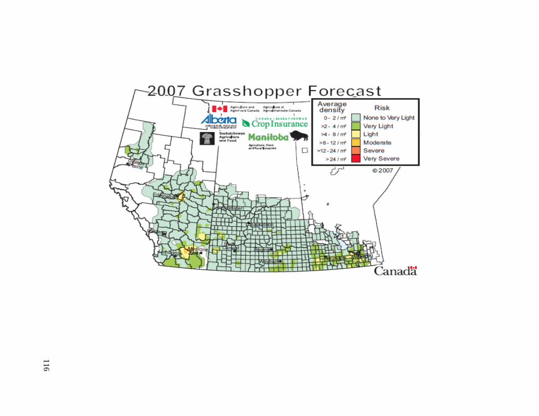
116

116

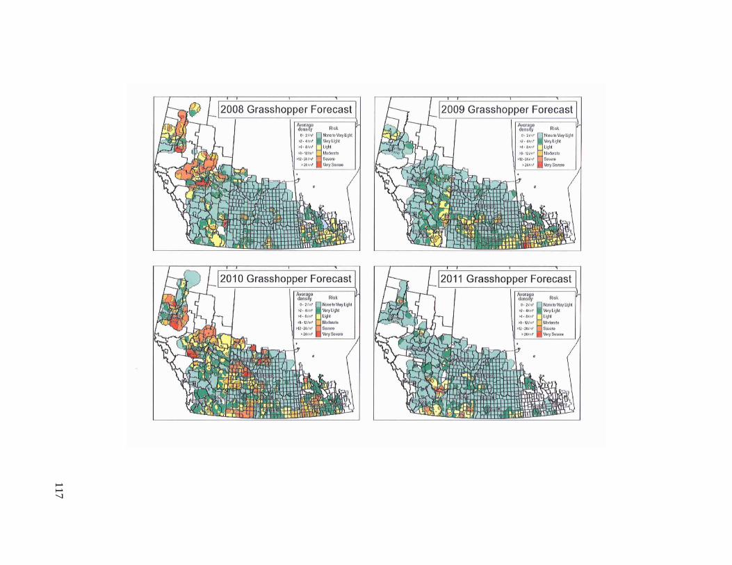
117

117

118

Appendix II:

Wheat Midge Forecasts for Saskatchewan and Prairies.

Taken from [161]

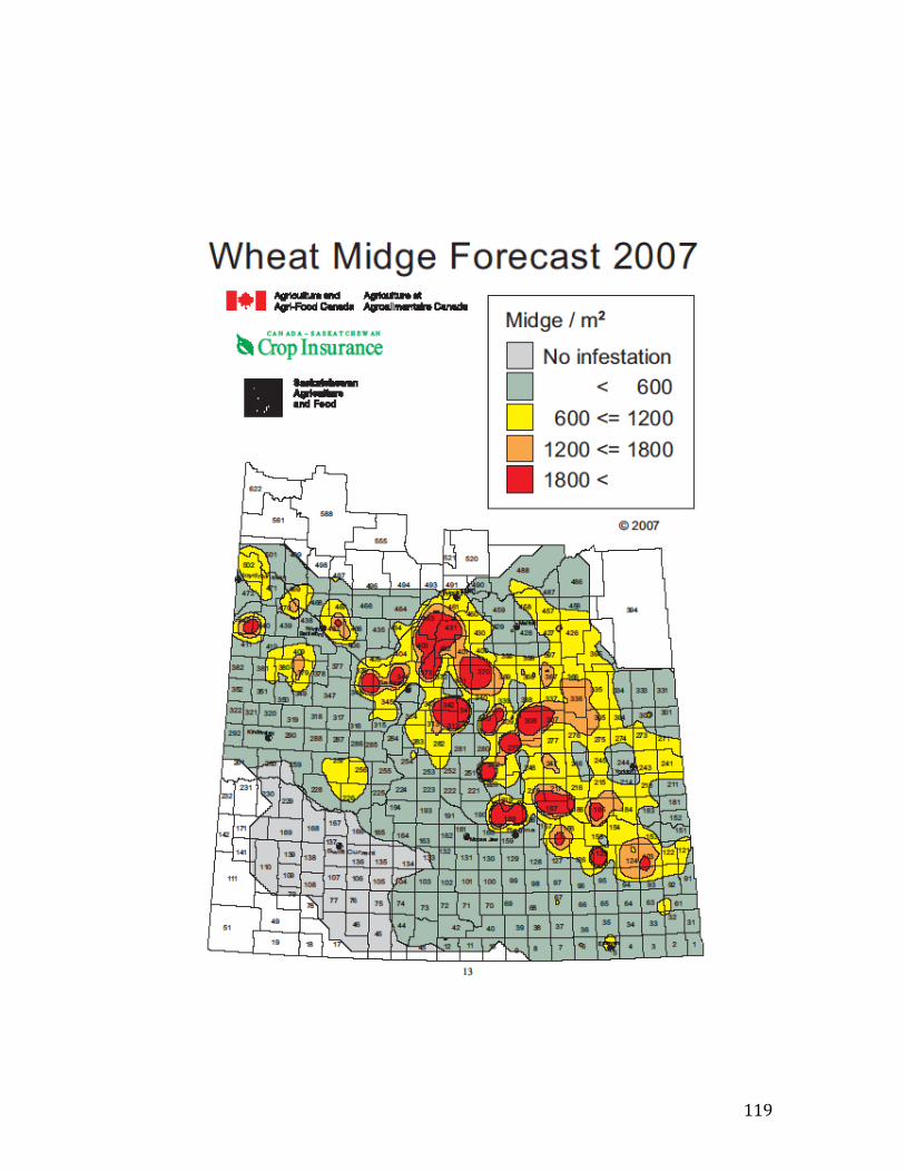
119

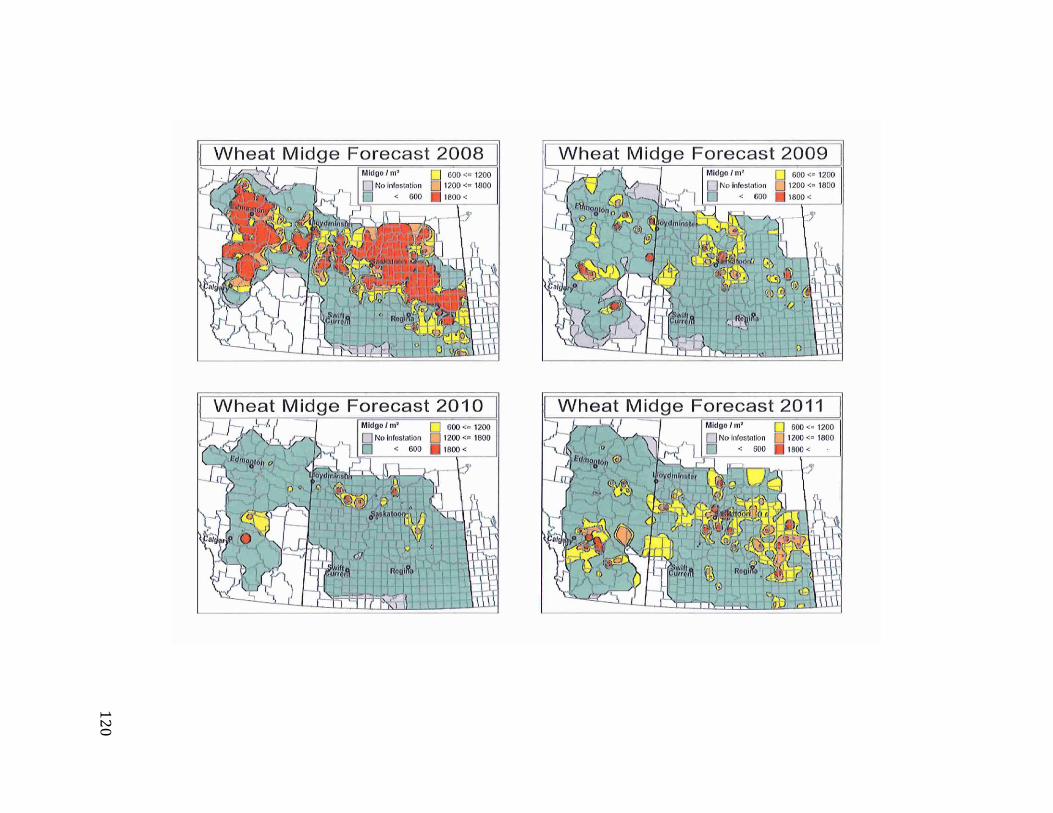
120

12

0

121

Appendix III:

Bertha Armyworm Forecasts for Saskatchewan and Prairies.

Taken from [161]

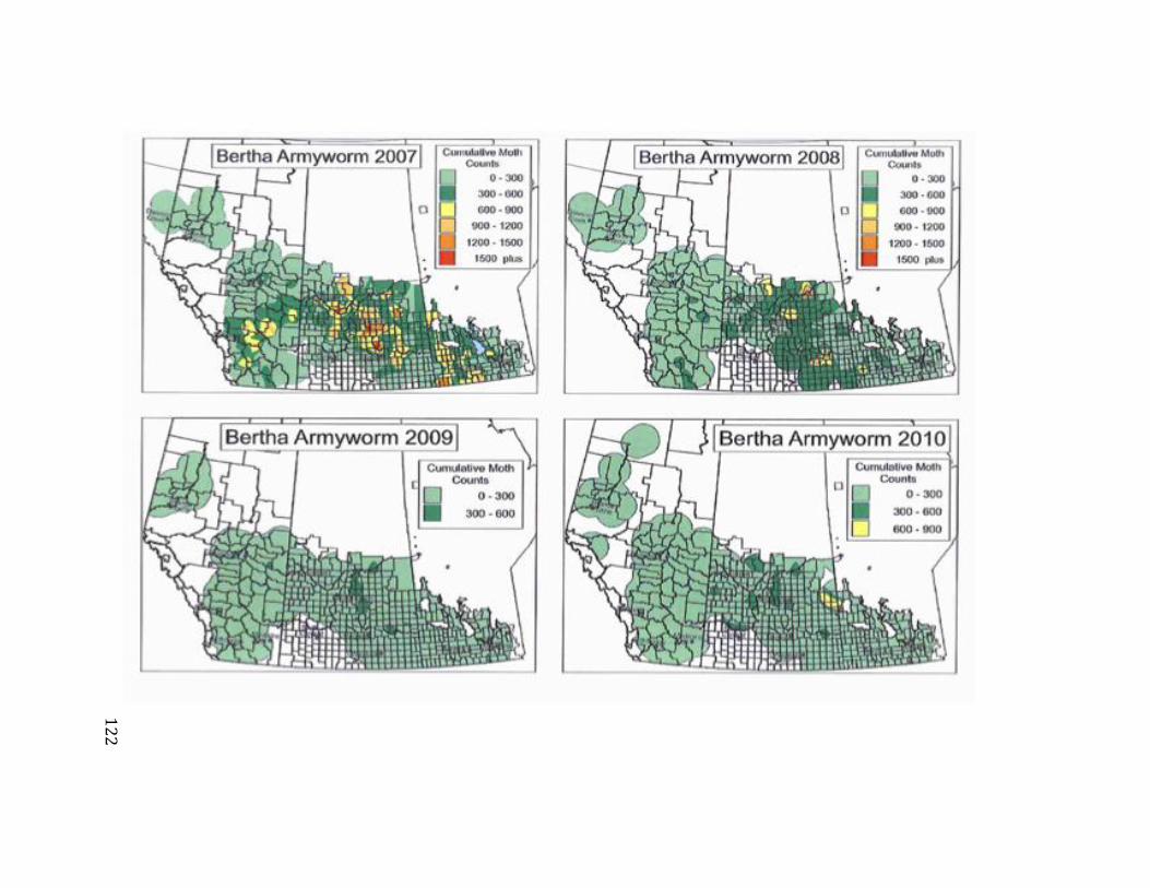
122

12

2

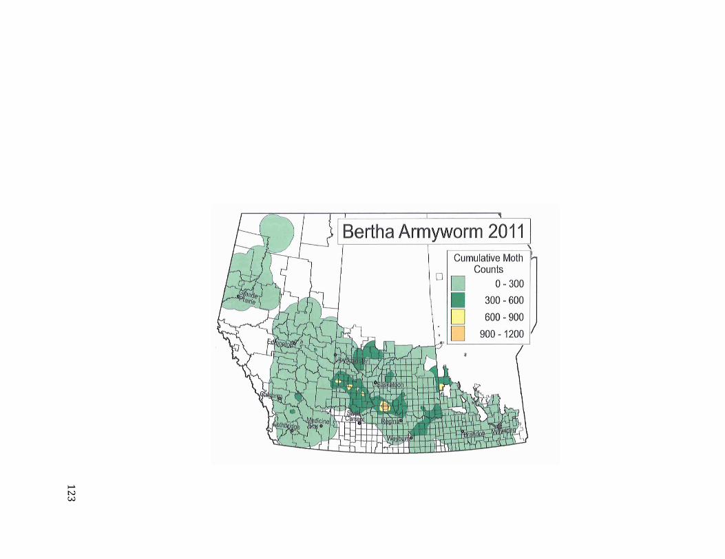
123

12

3