Atmospheric Environment 37 (2003) 4381–4392

Atmospheric aerosol over Finnish Arctic: source analysisby the multilinear engine and the potential source

contribution function

Tarja Yli-Tuomia, Philip K. Hopkea,*, Pentti Paaterob, M. Shamsuzzoha Basuniac,Sheldon Landsbergerc, Yrj .o Viisanend, Jussi Paaterod

aDepartment of Chemical Engineering, Clarkson University, Box 5708, Potsdam, NY 13699-5708, USAbDepartment of Physical Sciences, University of Helsinki, P.O. Box 64, FIN-00014, Finland

cNuclear Engineering Teaching Lab, University of Texas, Pickle Research Campus, Building 159, R-9000, Austin, TX 78712, USAdAir Quality Division, Finnish Meteorological Institute, P.O. Pox 503, FIN-00101 Helsinki, Finland

Received 30 January 2003; accepted 3 July 2003

Abstract

Week-long samples of total suspended particles were collected between 1964 and 1978 from Kevo at the Finnish

Arctic and analyzed for a number of chemical species. The chemical composition data was analyzed using a mixed

2-way/3-way model. The results of receptor modeling were connected with the back trajectory data in a Potential

Source Contribution Function analysis to determine the likely source areas. Nine sources, namely silver emissions, coal/

oil shale combustion, biomass burning, non-ferrous smelters (two sources), crustal elements from remote sources, excess

silicon from local sources, sea salt particles and biogenic sulfur emissions from marine algae were found. Although the

emissions from industrial areas in the Kola Peninsula had an effect on the concentration of anthropogenic pollutants at

Kevo, the highest concentrations during winter were transported from the sources in the mid-latitudes. The yearly

strength of the biogenic sulfur emissions showed no dependence on the Northern Hemisphere temperature anomaly and

thus, a climatic feedback loop could not be confirmed.

r 2003 Elsevier Ltd. All rights reserved.

Keywords: Arctic pollution; Receptor models; Multilinear engine; Potential source contribution function; Biogenic sulfur emissions

1. Introduction

The Arctic aerosol has been a subject of active

research since 1970. However, most of the studies have

been done on an episodic basis. There are no continuous

long-term measurements of the composition of airborne

particles prior to 1980. Especially, there has been no

long-term data with chemical composition from the

European Arctic, while several studies have been

conducted in the North American Arctic. It has been

found that mainly European and Asian emissions effect

to the pollutant concentrations in the Arctic, while the

North American sources have less important roles (e.g.

Raatz and Shaw, 1984; Ottar et al., 1986; Cheng et al.,

1993; Xie et al., 1999c). In this study, samples of total

suspended particles collected from Kevo in the Finnish

Arctic between 1965 and 1977 have been analyzed. Kevo

is located close to the Kola Peninsula, one of the most

polluted areas in the world. The emissions and effects of

large Ni–Cu smelters, apatite processing plant and

mines, Al smelter, iron ore mines and mills, and

Murmansk, a large harbor town with related industries,

have been widely studied (e.g. NILU, 1984; Sivertsen

et al., 1992; Tuovinen et al., 1993; Buznikov et al., 1995;

ARTICLE IN PRESS

AE International – Europe

*Corresponding author. Fax: +1-315-268-4410.

E-mail address: hopkepk@clarkson.edu (P.K. Hopke).

1352-2310/$ - see front matter r 2003 Elsevier Ltd. All rights reserved.

doi:10.1016/S1352-2310(03)00569-7

Jaffe et al., 1995; Kelley et al., 1995; Ahonen et al., 1997;

Reimann et al., 1998; Virkkula et al., 1999; Lupu and

Maenhaut, 2002). Ricard et al. (2002a, b) have studied

aerosol chemistry at Sevettijarvi in Finnish Lapland

between September 1997 and June 1999.

Charlson et al. (1987) suggested that biological

regulation of the climate is possible through the effects

of temperature and sunlight on phytoplankton popula-

tion. Since this kind of climatic feedback loop would

affect the global climate, biogenic sulfur emissions and

the concentration of biogenic sulfate and its tracer,

methane sulfonate, in the atmosphere have been

previously investigated in several studies (e.g. Bates

et al., 1992; Li et al., 1993a, b; Li and Barrie, 1993;

Hopke et al., 1995; Norman et al., 1999). At Alert in the

Canadian Arctic, the year-to-year intensity of a factor

describing biogenic sulfur emission was highly corre-

lated with the northern hemispheric temperature anom-

aly (Xie et al., 1999a, b). One objective for this study has

been to test the hypothesis that there would be a

relationship between biogenic sulfur emissions and

temperature.

The chemical composition data from Kevo has been

analyzed using the Multilinear Engine (ME) and the

potential source contribution function (PSCF) methods

to determine the source types, the temporal variation in

the source contributions, and source areas.

2. Sampling and chemical analyses

The Finnish Meteorological Institute (FMI) has been

collecting aerosol samples in northern Finland at Kevo

(69�450N, 27�020E) since October 1964. The topography

of the surrounding area is characterized by gently

sloping fell highlands with river valleys. The elevation

is mostly between 100 and 400m above sea level. The

area is sparsely populated (0.4 inhab. km�2). In the

summer, the sun shines without setting from mid-May

till the end of July, and remains below the horizon from

late November to mid-January. The ground is covered

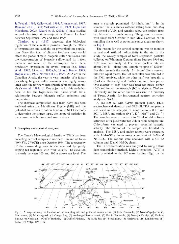
with snow from October to mid-May. Location of the

sampling site as well as potential source areas are shown

in Fig. 1.

The reason for the aerosol sampling was to monitor

natural and artificial radioactivity in the air. In this

study the weekly samples of total suspended particles

collected on Whatman 42 paper filters between 1964 and

1978 have been analyzed. The collection flow rate was

about 7m3 h�1 giving total sample volume of 1200m3.

For this research the weekly 12� 14 cm2 filters were cut

into two equal pieces. Half of each filter was retained in

the FMI archives, while the other half was brought to

Clarkson University and further cut into two pieces.

One quarter of each filter was used for black carbon

(BC) and ion chromatograph (IC) analysis at Clarkson

University and the other quarter was sent to University

of Texas, Austin, for instrumental neutron activation

analysis (INAA).

A DX-500 IC with GP50 gradient pump, ED50

electrochemical detector and SRS-ULTRA suppressor

was used in the analysis of major anions (Cl� and

SO42�), MSA and cations (Na+, K+, Mg2+ and Ca2+).

The samples were extracted into 20ml of chloroform-

saturated ultra-pure water for 24 h in room temperature.

Chloroform was used to prevent potential bacterial

activity. The aliquot of the sample was filtrated for

analysis. The MSA and major anions were separated

with AS4A-SC column using a gradient of 5–28mM

Na2B4O7. The cations were analyzed with a CS12A

column and 22mM H2SO4 eluent.

The BC concentration was analyzed by using diffuse

light transmission method. Light attenuation (ATN) is

linearly related to the BC mass loading ðSBCÞ on the

ARTICLE IN PRESS

Fig. 1. A map showing the location of the sampling site and potential source areas. (1) Kola Peninsula, (2) Nikel-Zapoljarnij, (3)

Murmansk, (4) Monchegorsk, (5) Onega Bay, (6) Archangel/Severodvinsk, (7) Kanin Peninsula, (8) Novaya Zemlya, (9) Pechora

Basin, (10) Norilsk, (11) Gulf of Bothnia, (12) Gulf of Finland, (13) Baltic Sea, (14) Stockholm, (15) Harjavalta, (16) Landskrona, (17)

Kiev, (18) Volga, (19) Ural.

T. Yli-Tuomi et al. / Atmospheric Environment 37 (2003) 4381–43924382

filter by the relation:

ATN ¼ �100 ln ðI I�10 Þ ¼ BATNSBC; ð1Þ

where I0 is the light intensity after passing a blank filter,

I the light intensity after passing a particle-loaded filter

and BATN is the specific attenuation coefficient (Ballach

et al., 2001). In this study, a specific attenuation

coefficient of 15 cm2 g�1 was used according to the

recommendation of Hansen (2000).

The INAA analysis were performed at TRIGA

MARK II research reactor facility, University of Texas

at Austin. Three separate irradiations were performed

for each sample, following a counting by high purity

germanium (HPGe) gamma spectrometry system. The

elements analyzed were Al, Ca, Cl, Cu, Mn, Na, Ti and

V with 2min thermal short irradiation, Ag with 1min

and As, Br, Co, I, In, K, Sb, Si, Sn, Zn, and W with

10min epithermal short irradiation. Each sample

occupied a volume of about 3ml in the pneumatic vial.

Inside the carrier vial another 2/5th dram vial was

placed on top of the filter containing about 500mg

sulfur powder. Sulfur powder was used to normalize the

neutron flux for each sample irradiation. New Whatman

42 paper filters were used as blanks in all chemical

analyses.

Details of the sampling, procedures of chemical

analyses and chemical composition were given by

Yli-Tuomi et al. (2003). To simplify the data analysis,

the data set has been truncated to calendar years

1965–1977 by eliminating samples from October to

December 1964 and January to March 1978.

3. Data analysis with the Multilinear Engine

The ME (Paatero, 1999) was developed for receptor

modeling. ME provides a new conceptual approach to

solving a variety of multilinear problems. Because of its

flexibility, ME has been used in several studies. For

example, Xie et al. (1999a) applied ME in the analysis of

Arctic aerosol data collected from Alert in the Canadian

Arctic. They found that a combination of bilinear and

trilinear factors produced better fit than pure 2- or 3-

way analyses carried out with Positive Matrix Factor-

ization by Xie et al. (1999b). Thus, the Kevo data was

analyzed with a mixed 2-way/3-way ME model using the

following equation:

xijk ¼XP

p¼1

tipkbjpckp þXR

r¼1

airbjðrþPÞckðrþPÞ þ eijk

¼ yijk þ eijk

i ¼ 1;y; I

j ¼ 1;y; J

k ¼ 1;y;K

0B@

1CA: ð2Þ

Each data point ðxijkÞ is expressed as a sum of P two-way

factors and R three-way factors. There are J chemical

species, I weeks in each year, and K years. The first term

represents the 2-way factors. The source contribution

term is divided into week-to-week variation (tipk), which

can be different for each year, and variation of the

strength across the years (ckp). The source composition

of a 2-way factor is presented by bjp: The second term

represents the trilinear part of the model. Unlike in the

2-way part, the week-to-week variation, air; is kept thesame in every year. The source composition of a 3-way

factor is given by bjðrþPÞ; while ckðrþPÞ represents the

variation across the years. The fitted value is denoted

with yijk; and eijk is the residual or the part of this

concentration which cannot be explained with the P þ R

sources.

The source composition factors were normalized so

that the sum of the species was one. The week-to-week

variation in the 3-way model was normalized to the

average of one over the year. The normalization of the

week-to-week variation of the 2-way factors was carried

out by coupling each year to a corresponding trilinear

factor with a constant week-to-week pattern and average

of one. The strength of the coupling was determined

with a coupling parameter. Depending on the value of

this parameter, the 2-way factors were actually between

pure trilinear PARAFAC model and pure bilinear

analysis of individual years. An intermediate value of

0.5 was found to be the best for the Kevo data.

Since there is less rotational freedom in a trilinear model

than in a bilinear model, the aspect of trilinearity

incorporated to the 2-way factors increased the stability

of the model and resulted in more reasonable source

compositions.

Determining the best fit according to Eq. (1) is

equivalent to solving the appropriate minimization

problem

miny

Qðx; s; yÞ; ð3Þ

where

Qðx; yÞ ¼XM

i¼1

ei

si

� 2

¼XM

i¼1

xi � yi

si

� 2

; ð4Þ

where M denotes the total number of measured values

and auxiliary equations. The value si is the uncertainty

of the measured value xi; while yi is the fitted value. All

sources were constrained to have non-negative species

concentration, and no sample was allowed to have

negative source contribution. The uncertainty of the

measured value depends on the analytical uncertainty

(C1) as well as on the modeling error (C3). The use of

point-by-point error estimates as the weight of the data

points improves the fit since more accurate values get

more weight than less accurate values. The accuracy

depends on the analyzed species as well as on its

concentration level. The analytical uncertainty was

obtained from the chemical analysis and a modeling

ARTICLE IN PRESST. Yli-Tuomi et al. / Atmospheric Environment 37 (2003) 4381–4392 4383

error (C3) of 15% was used. For concentrations higher

than the detection limit (DL), the uncertainty si was

computed as

si ¼ C1þ C3 si ; ð5Þ

where si ¼ max ðjxi j; jyi jÞ:For concentrations below the detection limit (BDL),

the DL was used as the xi value and the C1 for these

points was 5/6 DL. If the fitted value yi was above the

data value, the data value attempted to pull the fit down

towards itself (DL value), using si computed from

Eq. (5) with si ¼ jxi j: If, however, the fitted value was

below the data value, this data point got zero weight, i.e.

the data value did not pull the fitted value up towards

itself. Based on the plot of analytical uncertainty of

cobalt versus Co concentration, a C1 value of 5/6 DL

was too small and C1=DL was used for Co.

ME was used in a robust mode so that for any data

point for which the residual exceeded 4 times the error

estimate, the value was processed as an extreme value

and its weight was decreased.

Samples from 1965 to 1977 were arranged into 3-way

data array with 22 chemical species in 52 weekly samples

in each of the 13 years. Because there are approximately

52.2 weeks in a year, two samples had to be removed to

get the 22� 52� 13 array. The removed weeks were

selected in a way that the dates of the corresponding

weeks of different years matched as close as possible.

The removed samples were 25 January 72–1 January 73

and 27 December 76–3 January 77. Three samples, for

which the collection time was 2 or 3 weeks instead of one

week, were divided to weekly samples, all having the

same data values. They were weighted down by

increasing the uncertainty by a factor of 3. Geometric

mean values were used to substitute for missing samples

and 3-fold uncertainties were used for these points.

Since only about 70% of the variation of Co, Sb, Ti

and Mg concentrations in the samples was explained in

analysis with a pure bilinear model, it appears there is

larger uncertainty associated with these species and they

were weighted down by a factor of 3.

4. Potential source contribution function analysis

4.1. Trajectory data

The three-dimensional HYbrid Single-Particle La-

grangian Integrated Trajectory (HYSPLIT4) model

(March 2002 version; Draxler and Hess, 1997, 1998)

was used to reconstruct the air parcel movement. The

movement was described by segment endpoint coordi-

nates in terms of latitude and longitude of each point.

Five-day backward trajectories starting at height of

500m above the ground level using the vertical mixing

model were computed every day at 6 and 18 UTC

producing 14 trajectories per sample. The computations

were performed at the NOAA web site (http://www.

arl.noaa.gov/ready/sec/hysplit4.html) using archived

meteorological data set (REANALYSIS).

4.2. Potential source contribution function

PSCF analysis utilizes both chemical and back

trajectory data for each filter sample. The whole

geographic region covered by the trajectories was

divided into an array of 2.5� � 2.5� grid cells. This grid

cell covered latitudes from 40� to 90� North and

longitudes from �150� East to 150� West. If a trajectory

segment endpoint lies in the ijth cell, the trajectory is

assumed to collect material emitted in the cell. Once

the material is incorporated into the air parcel, it is

assumed to be transported along the trajectory to the

receptor site.

In PSCF analysis, if a trajectory is connected to a

sample which has contribution higher than a selected

criterion value, all sequence endpoints of this trajectory

are considered to be ‘‘high’’. For each cell the ratio of

high points (mij) to total points (nij) within the cell is

calculated

PSCFij ¼mij

nij

; ð6Þ

where PSCFij is the conditional probability that an air

parcel that passed through the ijth cell had a high

concentration upon arrival at the receptor site. A high

ratio in a cell indicates a potential source area.

There are artifacts in the PSCF analysis. If the total

number of endpoints in a cell is small, high points may

result in a high PSCFij value with a high uncertainty. In

order to minimize this artifact, Cheng et al. (1993)

multiplied the PSCF values with an arbitrary weight

function W ðnijÞ to better reflect the uncertainty in the

values for these cells. A similar approach have been used

for other PSCF calculation studies (Hopke et al., 1995;

Polissar et al., 2001a, b). Also for Kevo, a weight

function was applied for cells in which the total number

of endpoints was less than about three times the average

number of the endpoints per cell

W ðnijÞ ¼ 1:0; if 1800pnij

0:7; if 200pnijo1800

0:4; if 100pnijo200

0:2; if nijo100 ð7Þ

Local sources near the receptor site can cause high

concentration to the samples regardless of the direction

from which the airmass is coming. Usually no clear

source areas can be found in PSCF analysis for local

sources. A long sampling time gives rise to another

artifact. Within a week, there can be trajectories coming

from source areas as well as clean areas. If the

ARTICLE IN PRESST. Yli-Tuomi et al. / Atmospheric Environment 37 (2003) 4381–43924384

concentration in this sample is high, the number of

‘‘polluted’’ endpoints assigned to clean areas increases,

while low concentration samples may decrease the PSCF

values in source areas. However, this same problem

existed for the samples collected at Alert. At Alert,

week-long samples were collected with a high volume

sampler without particle size segregation. Although

there are trajectories both source and non-source areas

during the long sampling interval, it was possible to

obtain reasonable results and identify a number of

major sources (Cheng et al., 1993; Hopke et al., 1995;

Xie et al., 1999c).

The PSCF analysis were performed on all nine sets of

factor contribution. The averages of the sample-to-

sample source contribution values were used as the

criteria values. For factors that have a clear seasonal

variation, additional analyses using only the months

with high contribution were performed.

5. Results and discussion

The mixed models that were examined included seven

2-way and one 3-way model (abbreviated as 7+1); 6+2;

5+3; 5+1; 6+1; 8+1 and 9+1 models. Each model

was started from 20 pseudorandom values. The most

reasonable result was found with nine factors including

one trilinear factor that described biogenic sulfur. Before

running the mixed 2-way/3-way model, the data was

analyzed with a basic bilinear model. The result of the

mixed model was close to the bilinear results, but the

trilinear aspect stabilized the model and an additional

factor for crustal elements was found.

Although the factors provided by the ME were

physically interpretable, some rotational ambiguity still

existed and a priori information was used to limit the

rotational freedom in the model. More specifically, some

elements were pulled down from factors where they

should not appear, for example, crustal elements from

the sea salt factor. These rotations had only minor effect

on the Q value, mass fractions inside the factors, the

source contributions or source areas.

The source profiles (term b in Eq. (2)) after the

rotations are shown in Fig. 2, while the sample-to-

sample variation of mass contributions (tc or ac in

Eq. (2)) are presented in Fig. 3. The mass contributions

represent mass contributions (mass m�3) for the aerosol

mass determined by chemical species included in ME not

the measured mass since the total mass in unknown. The

variation of yearly strength (term c in Eq. (2)) of the

factors is shown in Fig. 4.

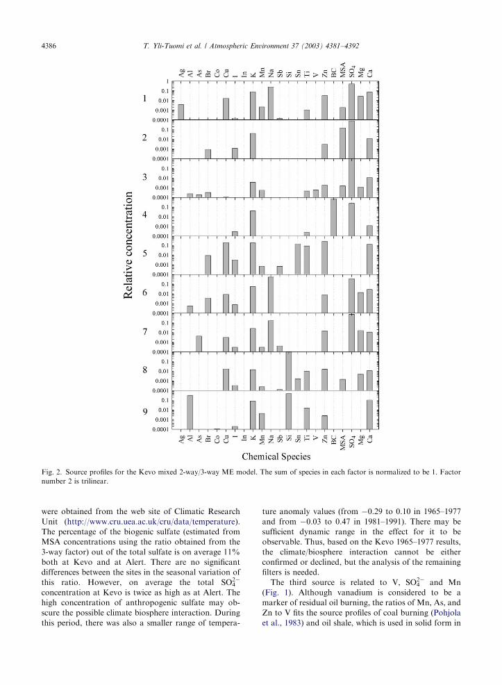
Based on the pure bilinear model, the first factor

describes about 90% of the variation of silver concen-

trations ando10% of variation in any other species. An

unique factor for silver was expected since the time trend

differs from other constituents. Silver was included in

the model since the highest concentrations coincided

with high Br and I concentrations. These high values

might be caused by reactions of particulate silver on the

filter with gaseous Br and I compounds. By including

Ag, the effect of this possible artifact was minimized.

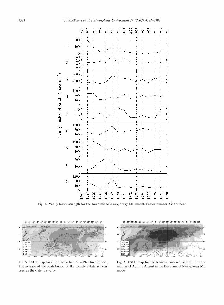
The variation of the yearly factor strength in Fig. 4

shows a steep decrease from 1965 to 1967 and elevated

concentrations for years from 1967 to 1971. The PSCF

result for the whole data set does not reveal any areas of

potential sources. PSCF analysis of a subset of data

from 1965 to 1971 (Fig. 5) shows possible source areas in

the Barents Sea between the Kola Peninsula and the

Kanin Peninsula and in the Onega Bay. PSCF values up

to 0.6 are shown in large areas in Europe and western

Russia, as well as around the Pechora Basin and Norilsk

areas. Thus, silver may originate from smelters, but still

the extremely high concentrations, up to 190 ngm�3

(Yli-Tuomi et al., 2003) remain unexplained.

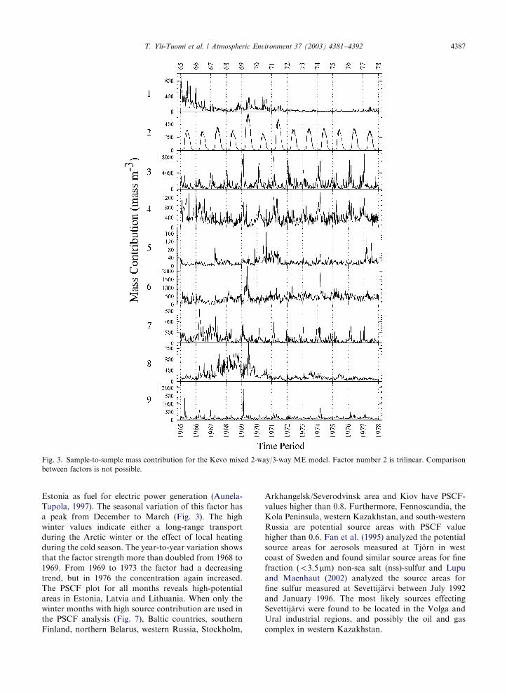
The second factor represents the biogenic sulfur

emissions. The seasonal variation of the biogenic

emissions has a nearly constant pattern from year-to-

year (Fig. 3). Thus, the emission is fitted with a 3-way

factor. High concentrations appear from April to

August and the PSCF plot for these months (Fig. 6)

shows strong source areas in the Barents Sea and

Norwegian Sea, as well as in the Gulf of Bothnia and

Gulf of Finland. The Kara Sea east of Novaya Zemlya,

the Baltic Sea and the area in front of the South-East

coast of Greenland are also likely source areas. In

addition to the sea areas, Norway, Sweden, Finland, the

Kola Peninsula and Karelia have high PSCF values. The

high values over the land can indicate terrestrial sources

(wetlands, freshwater, soil and vegetation) or more likely

pathways of air from sea.

The ratio of MSA to sulfate concentration for the

biogenic factor is 0.18. Although the ratio is higher than

that found in the pure bilinear analysis (0.13), it is low

compared to ratios observed at Alert in the Canadian

Arctic. In the mixed 2-way/3-way analysis of Alert data

collected between September 1980 and August 1991, the

MSA/SO42� was 0.31 in the biogenic factor (Xie et al.,

1999a). This result is consistent with the results of

isotope ratio analysis with average MSA/biogenic SO42�

of 0.3170.11 from June through September in Arctic

regions (Norman et al., 1999). The MSA to biogenic

sulfate ratio has been observed to be higher at colder

temperatures (Li and Barrie, 1993 and references there-

in). Since Kevo is located further south than Alert, the

lower MSA/biogenic SO42� ratio is consistent with the

previous observations.

Xie et al. (1999a, b) found a significant correlation

between the yearly strength of the 3-way biogenic factor

and the Northern Hemisphere temperature anomaly

linking the biogenic activity to the average temperature.

No such correlation can be observed in the Kevo data.

The Northern Hemisphere temperature anomaly values

ARTICLE IN PRESST. Yli-Tuomi et al. / Atmospheric Environment 37 (2003) 4381–4392 4385

were obtained from the web site of Climatic Research

Unit (http://www.cru.uea.ac.uk/cru/data/temperature).

The percentage of the biogenic sulfate (estimated from

MSA concentrations using the ratio obtained from the

3-way factor) out of the total sulfate is on average 11%

both at Kevo and at Alert. There are no significant

differences between the sites in the seasonal variation of

this ratio. However, on average the total SO42�

concentration at Kevo is twice as high as at Alert. The

high concentration of anthropogenic sulfate may ob-

scure the possible climate biosphere interaction. During

this period, there was also a smaller range of tempera-

ture anomaly values (from �0.29 to 0.10 in 1965–1977

and from �0.03 to 0.47 in 1981–1991). There may be

sufficient dynamic range in the effect for it to be

observable. Thus, based on the Kevo 1965–1977 results,

the climate/biosphere interaction cannot be either

confirmed or declined, but the analysis of the remaining

filters is needed.

The third source is related to V, SO42� and Mn

(Fig. 1). Although vanadium is considered to be a

marker of residual oil burning, the ratios of Mn, As, and

Zn to V fits the source profiles of coal burning (Pohjola

et al., 1983) and oil shale, which is used in solid form in

ARTICLE IN PRESS

Fig. 2. Source profiles for the Kevo mixed 2-way/3-way ME model. The sum of species in each factor is normalized to be 1. Factor

number 2 is trilinear.

T. Yli-Tuomi et al. / Atmospheric Environment 37 (2003) 4381–43924386

Estonia as fuel for electric power generation (Aunela-

Tapola, 1997). The seasonal variation of this factor has

a peak from December to March (Fig. 3). The high

winter values indicate either a long-range transport

during the Arctic winter or the effect of local heating

during the cold season. The year-to-year variation shows

that the factor strength more than doubled from 1968 to

1969. From 1969 to 1973 the factor had a decreasing

trend, but in 1976 the concentration again increased.

The PSCF plot for all months reveals high-potential

areas in Estonia, Latvia and Lithuania. When only the

winter months with high source contribution are used in

the PSCF analysis (Fig. 7), Baltic countries, southern

Finland, northern Belarus, western Russia, Stockholm,

Arkhangelsk/Severodvinsk area and Kiov have PSCF-

values higher than 0.8. Furthermore, Fennoscandia, the

Kola Peninsula, western Kazakhstan, and south-western

Russia are potential source areas with PSCF value

higher than 0.6. Fan et al. (1995) analyzed the potential

source areas for aerosols measured at Tj .orn in west

coast of Sweden and found similar source areas for fine

fraction (o3.5mm) non-sea salt (nss)-sulfur and Lupu

and Maenhaut (2002) analyzed the source areas for

fine sulfur measured at Sevettij.arvi between July 1992

and January 1996. The most likely sources effecting

Sevettij.arvi were found to be located in the Volga and

Ural industrial regions, and possibly the oil and gas

complex in western Kazakhstan.

ARTICLE IN PRESS

Fig. 3. Sample-to-sample mass contribution for the Kevo mixed 2-way/3-way ME model. Factor number 2 is trilinear. Comparison

between factors is not possible.

T. Yli-Tuomi et al. / Atmospheric Environment 37 (2003) 4381–4392 4387

ARTICLE IN PRESS

Fig. 4. Yearly factor strength for the Kevo mixed 2-way/3-way ME model. Factor number 2 is trilinear.

Fig. 5. PSCF map for silver factor for 1965–1971 time period.

The average of the contribution of the complete data set was

used as the criterion value.

Fig. 6. PSCF map for the trilinear biogenic factor during the

months of April to August in the Kevo mixed 2-way/3-way ME

model.

T. Yli-Tuomi et al. / Atmospheric Environment 37 (2003) 4381–43924388

The fourth factor has high concentration of BC and

potassium (Fig. 2) and thus, it is thought to be

associated to biomass burning (wood smoke). The

yearly strength of this factor decreases sharply in 1967,

but has increased steadily after that (Fig. 4). The PSCF

plot for the whole data set does not show any clear

source areas. The source contribution has its highest

values from January to March (Fig. 3) and the PSCF

map for these months (Fig. 8) shows potential source

areas in south-east Finland, southern Karelia and south-

west Russia.

The fifth factor describes the emissions from non-

ferrous metal smelters. There is no obvious seasonal

variation in the source contribution of this source

(Fig. 3), but the concentrations are higher from the

end of 1969 to mid-1971 (Fig. 4). The lack of seasonal

variation indicates that there is no significant pattern in

the emission strength and that the concentration at

Kevo does not depend on the long-range transport

during the Arctic winter. Thus, the smelters in the Kola

Peninsula would be likely sources. However, the

industrial areas of Nikel-Zapoljarnij and Monchegorsk

do not have high values in the PSCF analysis. Based on

continuous SO2 monitoring, the effect of the Kola

Peninsula emissions to Norwegian and Finnish Arctic

has been found to be episodic with typical duration of 2–

24 h (Sivertsen et al., 1992; Ahonen et al., 1997; Virkkula

et al., 1999). The mixture of ‘‘polluted’’ and ‘‘clean’’

trajectories within the week-long sampling period lowers

the resolution of the PSCF analysis. The areas with

highest source potentials are in southern Finland,

Sweden and Norway, Estonia, Latvia and area south

from the Kola Peninsula (Fig. 9). In the analysis of

Norwegian moss survey, Berg and Steinnes (1997) found

high metal concentrations around the smelters in

western Norway. In southern Finland Cu and Ni are

emitted from the Harjavalta smelter, while in Land-

skrona in southern Sweden, there is a secondary smelter

for lead and tin products (Boliden Bergs .oe, 2002).

Factor number six is characterized by high concentra-

tion of Na, Br, I and Mg (Fig. 2) and thus it describes

the sea salt particles. There are only slight variations in

the yearly strength of this factor (Fig. 4). Also the

seasonal variation is relatively small (Fig. 3). The areas

of highest source potentials are the Barents Sea,

Norwegian Sea and the Arctic Sea north from Novaya

Zemlya and Norilsk (Fig. 10). The correlation of sulfate

coming from sea salt with Na and other related elements

generated a sea salt factor such that sea salt and non-sea

salt sulfate are separated by the analysis in the same way

biogenic sulfate is separated from the anthropogenic

sulfate.

Factor seven is characterized by arsenic (Fig. 2). As is

emitted from non-ferrous metal smelters as well as Sn,

Cu, In and Zn, which were explained by factor 5.

However, As has lower boiling point than elements in

the fifth factor. Arsenic has been found to occur

predominantly in fine particles in the aerosol in the

Monchegorsk region (Kelley et al., 1995). The particle

size distribution affects the dispersion of the particles in

the atmosphere and thus the source areas are different.

ARTICLE IN PRESS

Fig. 8. PSCF plot for the wood burning factor during the

months of January to March in the Kevo mixed 2-way/3-way

ME model.

Fig. 9. PSCF plot for non-ferrous metal smelter 1 factor in the

Kevo mixed 2-way/3-way ME model.

Fig. 10. PSCF plot for sea salt factor in the Kevo mixed 2-way/

3-way ME model.

Fig. 7. PSCF plot for the coal/oil shale factor during the

months of December to March in the Kevo mixed 2-way/3-way

ME model.

T. Yli-Tuomi et al. / Atmospheric Environment 37 (2003) 4381–4392 4389

This factor has had high contribution during 1966 and

1967 (Fig. 4), otherwise its yearly strength has only

slight variations. The PSCF analysis for all months

shows potential source areas in Russia west from the

Urals, southern Finland and Baltic countries. The high

winter values (Fig. 3) seems to originate mainly from the

Kola Peninsula and Karelia, although there are areas of

high potential also in Baltic countries and most of

Belarus (Fig. 11). The southern end of the Urals is

consistent with the location of Ni–Cu smelters. The

source areas in Russia are similar with the results of Fan

et al. (1995). Lupu and Maenhaut (2002) associated high

arsenic loads at Sevettij.arvi with air transported from

the Kola Peninsula, Pechora Basin, and the Ural region.

The eighth factor explains the excess silicon, which

was observed from 1966 to 1969 (Yli-Tuomi et al.,

2003). The PSCF analysis shows no potential source

areas for this factor indicating that the Si emission is of

local origin. The emission might be related to the

construction work near the sampling site. The time

shows elevated values in the late 1960s when construc-

tion was occurring at the site.

In the ninth factor, the crustal elements are present in

ratios (X/Al) close to the typical crustal composition and

thus it represents windblown dust. The highest

contributions, however, occur during the winter time

(Fig. 3), when the ground in the Arctic areas is covered

by snow. This indicates that the particles are transported

from remote areas. Pacyna and Ottar (1989) found that

the natural constituents in the Arctic aerosol in the

Norwegian Arctic is dust which is eroded from the

deserts in Asia and Africa during dust storms. These

dust storms typically occur in February to April and

thus, may be the origin of these high events. Because of

the transport pathways, the source areas are unlikely to

appear in the PSCF map (Fig. 12).

6. Conclusions

In the analysis of Kevo data with a mixed 2-way/3-

way ME model and PSCF method, a solution with 9

sources was found to give the best result. The factors

were associated to the following sources: silver emis-

sions, coal combustion, biomass burning, non-ferrous

smelters (two sources), crustal elements from remote

sources, excess silicon from local sources, sea salt

particles and biogenic sulfur emissions from marine

algae. Although the industrial areas in the Kola

Peninsula are likely sources, they did not show high

potential in the PSCF analysis of the smelter factor

describing Sn, Cu, In and Zn emissions. The highest

concentrations during the winter and spring were caused

by long-range transport from mid-latitudes.

The biogenic emission was modeled as a trilinear

factor. A strong source area was found in the Barents

Sea in addition to the Norwegian Sea and the North

Atlantic, which have been pointed out in previous

studies. The ratio of MSA to sulfate in the biogenic

factor was 0.18. No relationship between the yearly

strength of the biogenic emissions and the Northern

Hemisphere temperature anomaly was found and thus,

the suggested climate-biosphere feedback loop remains

unconfirmed.

Acknowledgements

The work at Clarkson University and at the Uni-

versity of Texas at Austin were supported by Coopera-

tive Institute for Arctic Research.

References

Ahonen, T., Aalto, P., Rannik, .U., Kulmala, M., Nilsson, E.D.,

Palmroth, S., Ylitalo, H., Hari, P., 1997. Variations and

vertical profiles of trace gas and aerosol concentration and

CO2 exchange in Eastern Lapland. Atmospheric Environ-

ment 31 (20), 3351–3362.

Aunela-Tapola L., 1997. Trace metal emissions from the

combustion of Estonian oil shale. Licentiate Thesis,

University of Kuopio, Department of Environmental

Sciences.

ARTICLE IN PRESS

Fig. 11. PSCF plot for non-ferrous metal smelter 2 factor (As

emissions) during the months of November to March in the

Kevo mixed 2-way/3-way ME model.

Fig. 12. PSCF plot for factor of crustal elements during the

months of February to April in the Kevo mixed 2-way/3-way

ME model.

T. Yli-Tuomi et al. / Atmospheric Environment 37 (2003) 4381–43924390

Ballach, J., Hitzenberger, R., Shultz, E., Jaeschke, W., 2001.

Development of an improved optical transmission technique

for black carbon (BC) analysis. Atmospheric Environment

35, 2089–2100.

Bates, T.S., Lamb, T.S., Guenther, A., Dignon, J., Stoiber,

R.E., 1992. Sulfur emissions to the atmosphere from

natural sources. Journal of Atmospheric Chemistry 14,

315–337.

Berg, T., Steinnes, E., 1997. Recent trends in atmospheric

deposition of trace elements in Norway as evident from the

1995 moss survey. The Science of the Total Environment

208, 197–206.

Boliden Bergs .oe, AB., 2002. http://www.bolidenbergsoe.se/eng/

foretag.htm. Accessed December 2002.

Buznikov, A.A., Payanskaya-Gvozdeva, I.I., Jurkovskaya,

T.K., Andreeva, E.N., 1995. Use of remote and ground

methods to assess the impacts of smelter emissions in the

Kola Peninsula. The Science of the Total Environment 160/

161, 285–293.

Charlson, R.J., Lovelock, J.E., Andreae, M.O., Warren, S.G.,

1987. Oceanic phytoplancton, atmospheric sulphur, Cloud

Albedo and climate. Nature 326 (16), 655–661.

Cheng, M.-D., Hopke, P.K., Barrie, L.A., Rippe, A., Olson,

M., Landsberger, S., 1993. Qualitative determination of

source regions of aerosol in Canadian High Arctic.

Environmental Science and Technology 27 (10), 2063–2071.

Draxler, R.R., Hess, G.D., 1997. Description of the

HYSPLIT 4 Modeling System. NOAA Technical Memor-

andum ERL ARL-224, December, 24p.

Draxler, R.R., Hess, G.D., 1998. An overview of the

HYSPLIT 4 modeling system for trajectories, dispersion

and deposition. Australian Meteorological Magazine 47,

295–308.

Fan, A., Hopke, P.K., Raunemaa, T., .Oblad, M., Pacyna, J.M.,

1995. A study on the potential sources of air pollutants

observed at Tj .orn, Sweden. Environmental Science and

Pollution Research 2 (2), 107–115.

Hansen, A.D.A., 2000. Personal communication.

Hopke, P.K., Barrie, L.A., Li, S.-M., Cheng, M.-D., Li, C., Xie,

Y.-L., 1995. Possible sources and preferred pathways for

biogenic and Non-sea-salt sulfur for the high Arctic. Journal

of Geophysical Research 100 (D8), 16595–16603.

Jaffe, D., Cerundolo, B., Rickers, J., Stolzberg, R., Baklanov,

A., 1995. Deposition of sulfate and heavy metals on the

Kola Peninsula. The Science of the Total Environment 160/

161, 127–134.

Kelley, J.A., Jaffe, D.A., Baklanov, A., Mahura, A., 1995.

Heavy metals on the Kola Peninsula: aerosol size distribu-

tion. The Science of the Total Environment 160/161,

135–138.

Li, S.-M., Barrie, L.A., 1993. Biogenic sulfur aerosol in the

arctic troposphere: 1. Contributions to total sulfate. Journal

of Geophysical Research 98 (D11), 20613–20622.

Li, S.-M., Barrie, L.A., Sirois, A., 1993a. Biogenic sulfur

aerosol in the arctic troposphere: 2. Trends and seasonal

variations. Journal of Geophysical Research 98 (D11),

20623–20631.

Li, S.-M., Barrie, L.A., Talbot, R.W., Harris, R.C., Davidson,

C.I., Jaffrezo, J.-L., 1993b. Seasonal and geographic

variations of methanesulfonic acid in the Arctic tropo-

sphere. Atmospheric Environment A 27 (17/18), 3011–3024.

Lupu, A., Maenhaut, W., 2002. Application and comparison of

two statistical trajectory techniques for identification of

source regions of atmospheric aerosol species. Atmospheric

Environment 36, 5607–5618.

NILU (Norwegian Institute for Air Research), 1984. Emission

Sources in the Soviet Union. NILU 4/84.

Norman, A.L., Barrie, L.A., Toom-Saintry, D., Sirois, A.,

Krouse, H.R., Li, S.-M., Sharma, S., 1999. Sources of

aerosol sulphate at alert: apportionment using stable

isotopes. Journal of Geophysical Research 104 (D9),

11619–11631.

Ottar, B., Pacyna, J.M., Berg, T.C., 1986. Aircraft measure-

ments of air pollution in the Norwegian Arctic. Atmo-

spheric Environment 20 (1), 87–100.

Paatero, P., 1999. The multilinear engine—a table-driven, least

squares program for solving multilinear problems, including

the n-way parallel factor analysis model. Journal of

Computational and Graphical Statistics 8 (4), 854–888.

Pacyna, J.M., Ottar, B., 1989. Origin of natural constituents

in the Arctic aerosol. Atmospheric Environment 23 (4),

809–815.

Pohjola, V., Hahkala, M., H.as.anen, E., 1983. Kivihiilt.a,

Turvetta ja .Oljy.a K.aytt.avien L.amp .ovoimaloiden P.a.ast-

.oselvitys (Emission estimations of coal, peat and oil fired

power plants). VTT Tutkimuksia 231.

Polissar, A.V., Hopke, P.K., Harris, J.M., 2001a. Source

regions for atmospheric aerosol measured at Barrow,

Alaska. Environmental Science and Technology 35,

4214–4226.

Polissar, A.V., Hopke, P.K., Poirot, R.L., 2001b. Atmospheric

aerosol over Vermont: chemical composition and sources.

Environmental Science and Technology 35, 4604–4621.

Raatz, W.E., Shaw, G.E., 1984. Long range transport of

pollution aerosols into the Alaskan Arctic. Journal of

Climate and Applied Meteorology 23 (11), 1052–1064.

Reimann, C., Chekushin, V., Bogatyrev, I., Boyd, R.,

de Caritat, P., Dutter, R., Finne, T.E., Halleraker, J.H.,

Jæger, Ø., Kashulina, G., Lehto, O., Niskavaara, H.,

Pavlov, V., R.ais.anen, M.L., Strand, T., Volden, T.,

1998. Environmental geochemical atlas of the central

Barents region. Geological Survey of Norway, Trondheim,

Norway.

Ricard, V., Jaffrezo, J.L., Kerminen, V.M., Hillamo, R.E.,

Sillanp.a.a, M., Ruellan, S., Liousse, C., Cachier, H., 2002a.

Two years of continuous aerosol measurements in Northern

Finland. Journal of Geophysical Research-Atmosphere,

107(D11).

Ricard, V., Jaffrezo, J.L., Kerminen, V.M., Hillamo, R.E.,

Teinila, K., Maenhaut, W., 2002b. Size distributions and

modal parameters of aerosol constituents in northern

Finland during the European Arctic aerosol study. Journal

of Geophysical Research-Atmosphere, 107(D14).

Sivertsen, B., Makarova, T., Hagen, L.O., Baklanov, A.A.,

1992. Air Pollution in the Border Areas of Norway and

Russia. Lillestrom, NILU-Norwegian Institute for Air

Research, pp. 1–14.

Tuovinen, J.-P., Laurila, T., L.attil.a, H., Ryaboshapko, A.,

Brukhanov, P., Korolev, S., 1993. Impact of the sulphur

dioxide sources in the Kola Peninsula on air quality in

Northern Europe. Atmospheric Environment 27A (9),

1379–1395.

ARTICLE IN PRESST. Yli-Tuomi et al. / Atmospheric Environment 37 (2003) 4381–4392 4391

Virkkula, A., Aurela, M., Hillamo, R., M.akel.a, T., Pakkanen,

T., Maenhaut, W., Fran@ois, F., Cafmeyer, J., 1999.

Chemical composition of atmospheric aerosol in the

European subarctic: contribution of the Kola Peninsula

smelter areas, central Europe, and the Arctic Ocean. Journal

of Geophysical Research 104 (D19), 23681–23696.

Xie, Y.-L., Hopke, P.K., Paatero, P., Barrie, L.A., Li, S.-M.,

1999a. Identification of source nature and seasonal varia-

tions of Arctic aerosol by the multilinear engine. Atmo-

spheric Environment 33, 2549–2562.

Xie, Y.-L., Hopke, P.K., Paatero, P., Barrie, L.A., Li, S.-M.,

1999b. Identification of source nature and seasonal

variations of Arctic aerosols by positive matrix

factorization. Journal of the Atmospheric Sciences 56,

249–260.

Xie, Y.-L., Hopke, P.K., Paatero, P., Barrie, L.A., Li, S.-M.,

1999c. Locations and preferred pathways of possible

sources of Arctic aerosol. Atmospheric Environment 33,

2229–2239.

Yli-Tuomi, T., Venditte, L., Hopke, P.K., Basunia, M.S.,

Landsberger, S., Viisanen, Y., Paatero, J., 2003. Composi-

tion of the Finnish Arctic Aerosol: collection and analysis

of historic filter samples. Atmospheric Environment 37,

2355–2364.

ARTICLE IN PRESST. Yli-Tuomi et al. / Atmospheric Environment 37 (2003) 4381–43924392