ATEX CLASS FILES, VOL. XX, NO. X, AUGUST 201X 1

1041-4347 (c) 2018 IEEE. Personal use is permitted, but republication/redistribution requires IEEE permission. See http://www.ieee.org/publications_standards/publications/rights/index.html for more information.

This article has been accepted for publication in a future issue of this journal, but has not been fully edited. Content may change prior to final publication. Citation information: DOI 10.1109/TKDE.2018.2824328, IEEETransactions on Knowledge and Data Engineering

JOURNAL OF LATEX CLASS FILES, VOL. XX, NO. X, AUGUST 201X 1

Quantifying Differential Privacy in ContinuousData Release under Temporal Correlations

Yang Cao, Masatoshi Yoshikawa, Yonghui Xiao, and Li Xiong

Abstract—Differential Privacy (DP) has received increasing attention as a rigorous privacy framework. Many existing studies employtraditional DP mechanisms (e.g., the Laplace mechanism) as primitives to continuously release private data for protecting privacy ateach time point (i.e., event-level privacy), which assume that the data at different time points are independent, or that adversaries donot have knowledge of correlation between data. However, continuously generated data tend to be temporally correlated, and suchcorrelations can be acquired by adversaries. In this paper, we investigate the potential privacy loss of a traditional DP mechanismunder temporal correlations. First, we analyze the privacy leakage of a DP mechanism under temporal correlation that can be modeledusing Markov Chain. Our analysis reveals that, the event-level privacy loss of a DP mechanism may increase over time. We call theunexpected privacy loss temporal privacy leakage (TPL). Although TPL may increase over time, we find that its supremum may exist insome cases. Second, we design efficient algorithms for calculating TPL. Third, we propose data releasing mechanisms that convertany existing DP mechanism into one against TPL. Experiments confirm that our approach is efficient and effective.

Index Terms—Differential Privacy, Correlated data, Markov Model, Time series, Streaming data.

F

1 INTRODUCTION

W ITH the development of IoT technology, vast amountof temporal data generated by individuals are being

collected, such as trajectories and web page click streams.The continual publication of statistics from these temporaldata has the potential for significant social benefits such asdisease surveillance , real-time traffic monitoring and webmining. However, privacy concerns hinder the wider useof these data. To this end, differential privacy under continualobservation [1] [2] [3] [4] [5] [6] [7] [8] has received increasingattention because differential priavcy provides a rigorousprivacy guarantee. Intuitively, differential privacy (DP) [9]ensures that the change of any single user’s data has a“slight” (bounded in ε) impact on the change in outputs. Theparameter ε is defined to be a positive real number to controlthe level of privacy guarantee. Larger values of ε result inlarger privacy leakage. However, most existing works ondifferentially private continuous data release assume dataat different time points are independent, or attackers donot have knowledge of correlation between data. Example 1shows that temporal correlations may degrade the expectedprivacy guarantee of a DP mechanism.

Example 1. Consider the scenario of continuous data release withDP illustrated in Figure 1. A trusted server collects users’ loca-tions at each time point in Figure 1(a) and tries to continuouslypublish differentially private aggregates (i.e., the private countsof people at each location). Suppose that each user appears atonly one location at each time point. According to the Laplace

• Yang Cao, Xiong Li are with the Department of Math and ComputerScience, Emory University, Atlanta, GA, 30322.E-mail: {ycao31, lxiong}@emory.edu.

• Masatoshi Yoshikawa is with the Department of Social Informatics, KyotoUniversity, Kyoto, Japan, 606-8501.E-mail: [email protected].

• Yonghui Xiao is with Google Inc., Mountain View, CA, 94043E-mail: [email protected].

Manuscript received XXX; revised XXX.

t= 1 2 3 …u1 loc3 loc1 loc1 …u2 loc2 loc1 loc1 …u3 loc2 loc4 loc5 …u4 loc4 loc5 loc3 …

(a) Location Data (b) Road Network loc4

loc5loc3

(d) Differentially Private Counts(c) True Counts

t= 1 2 3 ..loc1 0 2 2 ..loc2 2 0 0 ..loc3 1 0 1 ..loc4 1 1 0 ..loc5 0 1 1 ..

t= 1 2 3 ..loc1 0 1 3 ..loc2 3 1 0 ..loc3 1 0 1 ..loc4 2 1 0 ..loc5 1 3 3 ..

LaplaceNoise

Count queries

Fig. 1. Continuous Data Release with DP under Temporal Correlations.

mechanism [10], adding Lap(2/ε) noise1 to perturb each countin Figure1(c) can achieve ε-DP at each time point. It is because themodification of each cell (raw data) in Figure 1(a) affects at mosttwo cells (true counts) in Figure 1(c), i.e., the global sensitivityis 2. However, it may not be true under the existence of temporalcorrelations. For example, due to the nature of road networks, usermay have a particular mobility pattern such as “always arrivingat loc5 after visiting loc4” (shown in Figure 1(b)), leading to thepatterns illustrated in solid lines of Figure 1(a)(c). Such temporalcorrelation can be represented as Pr(lt = loc5|lt−1 = loc4) = 1

where lt is the location of a user at time t. In this case, addingLap(2/ε) noise only achieves 2ε-DP because the change of onecell in Figure 1(a) may affect four cells in Figure 1(c) in the worstcase, i.e., the global sensitivity is 4.

Few studies in the literature investigated such potentialprivacy loss of event-level ε-DP under temporal correlationsas shown in Example 1. A direct method (without finelyutilizing the probability of correlation) involves amplifyingthe perturbation in terms of group differential privacy [11] [10],i.e., protecting the correlated data as a group. In Example 1,for temporal correlation Pr(lt = loc5|lt−1 = loc4) = 1, we can

1. Lap(b) denotes a Laplace distribution with variance 2b2.




protect the counts of loc4 at time t − 1 and loc5 at time t ina group by increasing the scale of the perturbation (usingLap(4/ε)) at each time point. However, this technique isnot suitable for probabilistic correlations to finely preventprivacy leakage and may over-perturb the data as a result.For example, regardless of whether Pr(lt = loci|lt−1 = loci) is1 or 0.1, it always protects the correlated data in a bundle.

Although a few studies investigated the issue of dif-ferential privacy under probabilistic correlations, existingworks are not appropriate for continuous data release becauseof two reasons. First, most of existing works focused oncorrelations between users (i.e., user-user correlation) ratherthan correlation between data at different time points (i.e.,temporal correlations). Yang et al. [12] proposed Bayesiandifferential privacy, which measures the privacy leakageunder probabilistic correlations between users using a Gaus-sian Markov Random Field without taking time factor intoaccount. Liu et al. [13] proposed dependent differential pri-vacy by introducing two parameters of dependence size andprobabilistic dependence relationship between tuples. It is notclear whether we can specify these parameters for tempo-rally correlated data since it is not commonly used prob-abilistic model. A concurrent work [17] proposed MarkovQuilt Mechanism when data correlation is represented by aBayesian Network (BN). Although BN is possible to modelboth user-user correlation (when the nodes in BN are indi-viduals) and temporal correlation (when the nodes in BN areindividual data at different time points), [17] assumes theprivate data are released only at one time. This is the secondmajor difference between our work and all above works:they focus on the setting of “one-shot” data release, whichmeans the private data are released only at one time. Tothe best of our knowledge, no study reported the dynamicalchange of the privacy guarantee in continuous data release.

In this work, we call the adversary with knowledge ofprobabilistic temporal correlations adversaryT . Rigorouslyquantifying and bounding the privacy leakage againstadversaryT in continuous data release remains a challenge.Therefore, our goal is to solve the following problems:

• How do we analyze the privacy loss of DP mechanismsagainst adversaryT ? (Section 3)

• How do we calculate such privacy loss efficiently?(Section 4)

• How do we bound such privacy loss in continuousdata release? (Section 5)

1.1 ContributionsOur contributions are summarized as follows.

First, we show that the privacy guarantee of data releaseat a single time is not on its own or static; instead, due to theexistence of temporal correlation, it may be increasing withprevious release and even future release. We first adopt acommonly used model Markov Chain to describe temporalcorrelations between data at different time points, whichincludes backward and forward correlations, i.e., Pr(lt−1

i |lti)and Pr(lti |lt−1

i ) where lti denotes the value (e.g., location)of user i at time t. We then define Temporal Privacy Leakage(TPL) as the privacy loss of a DP mechanism at time t againstadversaryT who has knowledge of the above Markov modeland observes the continuous data release. We show that

TPL includes two parts: Backward Privacy Leakage (BPL) andForward Privacy leakage (FPL). Intuitively, BPL at time t isaffected by previously releases that are from time 1 to t− 1,and FPL at time t will be affected by future releases thatare from time t + 1 to the end of release. We define α-differential privacy under temporal correlation, denoted as α-DPT , to formalize the privacy guarantee of a DP mechanismagainst adversaryT , which implies the temporal privacyleakage should be bounded in α. We prove a new form ofsequential composition theorem for α-DPT , which revealsinteresting connections among event-level DP, w-event DP[7] and user-level DP [4] [5].

Second, we design efficient algorithms to calculate TPLunder given backward and forward temporal correlations.Our idea is to transform such calculation into finding anoptimal solution of a Linear-Fractional Programming problem.This type of optimization can be solved by well-studiedmethods, e.g., simplex algorithm, in exponential time. Byexploiting the constraints of this problem, we propose fastalgorithms to obtain the optimal solution without directlysolving the problem. Experiments show our algorithms out-perform the off-the-shelf optimization software (CPLEX) byseveral orders of magnitude with the same optimal answer.

Third, we design novel data release mechanisms againstTPL effectively. Our scheme is to carefully calibrate the pri-vacy budget of the traditional DP mechanism at each timepoint to make them satisfy α-DPT . A challenge is that TPLis dynamically changing due to previous and even futureallocated privacy budgets so that α-DPT is hard to achieve.In our first solution, we prove that, even though TPL mayincrease over time, its supremum may exist when allocatinga calibrated privacy budget at each time. That is to say,TPL will never be greater than such supremum α no matterwhen the release ends. However, when the releases are tooshort (TPL is far from reaching its supremum), we may over-perturb the data. In our second solution, we design anotherbudget allocation scheme that exactly achieves α-DPT ateach time point.

Finally, experiments confirm the efficiency and effective-ness of our TPL quantification algorithms and data releasemechanisms. We also demonstrate the impact of differentdegree of temporal correlations on privacy leakage.

2 PRELIMINARIES

2.1 Differential Privacy

Differential privacy [9] is a formal definition of data privacy.Let D be a database and D′ be a copy of D that is differentin any one tuple. D and D′ are neighboring databases. Adifferentially private output from D or D′ should exhibitlittle difference.

Definition 1 (ε-DP). M is a randomized mechanism that takesas input D and outputs r, i.e., M(D) = r. M satisfies ε-differential privacy if the following inequality is true for any pairof neighboring databases D,D′ and all possible outputs r.

logPr(r ∈ Range(M)|D)

Pr(r ∈ Range(M)|D′) ≤ ε. (1)

The parameter ε, called the privacy budget, represents thedegree of privacy offered. A commonly used method toachieve ε-DP is the Laplace mechanism as shown below.




Theorem 1 (Laplace Mechanism). Let Q : D → R be astatistical query on database D. The sensitivity of Q is de-fined as the maximum L1 norm between Q(D) and Q(D′), i.e.,∆ = maxD,D′ ||Q(D) − Q(D′)||1. We can achieve ε-DP by addingLaplace noise with scale ∆/ε, i.e., Lap(∆/ε).

2.2 Privacy Leakage

In this section, we define the privacy leakage of a DPmechanism against a type of adversaries Ai, who targetsuser i’s value in the database, i.e., li ∈ [loc1, . . . , locn], andhas knowledge of DK = D−{li}. The adversaryAi observesthe private output r and attempts to distinguish whetheruser i’s value is locj or lock where locj , lock ∈ [loc1, . . . , locn].We define the privacy leakage of a DP mechanism w.r.t. suchadversaries as follows.

Definition 2. The privacy leakage of a DP mechanismM againstoneAi with a specific i and allAi, i ∈ U are defined, respectively,as follows in which li and l′i are two different possible values ofi-th data in the database.

PL0(Ai,M)def== sup

r,li,l′i

logPr(r|li, DK)

Pr(r|l′i, DK)

PL0(M)def== max∀Ai,i∈U

PL0(Ai,M) = supr,D,D′

logPr(r|D)

Pr(r|D′)

In other words, the privacy budget of a DP mechanismcan be considered as a metric of privacy leakage. The larger ε,the larger the privacy leakage. We note that a ε′-DP mecha-nism automatically satisfies ε-DP if ε′ < ε. For convenience,in the rest of this paper, when we say thatM satisfies ε-DP,we mean that the supremum of privacy leakage is ε.

2.3 Problem Setting

We attempt to quantify the potential privacy loss of a DPmechanism under temporal correlations in the context ofcontinuous data release (e.g., releasing private counts at eachtime as shown in Figure 1). For the convenience of analysis,let us assume the length of release time is T . Note that wedo not need to know the exact T in this paper. Users in thedatabase, denoted by U , are generating data continuously.Let loc = {loc1, . . . , locn} be all possible values of user’sdata. We denote the value of user i at time t by lti . Atrusted server collects the data of each user into the databaseDt = {lt1, . . . , lt|U|} at each time t (e.g., the columns in Figure1(a)). Without loss of generality, we assume that each usercontributes only one data point in Dt. DP mechanismsMt

release differentially private outputs rt independently atdifferent time t. For simplicity, we letMt to be the same DPmechanism but may with different privacy budgets at eacht ∈ [1, T ]. Our goal is to quantify and bound the potentialprivacy loss of Mt against adversaries with knowledge oftemporal correlations. We note that while we use locationdata in Example 1, the problem setting is general for tempo-rally correlated data. We summarize notations used in thispaper in Table 1.

Our problem setting is identical to differential privacyunder continual observation in the literature [1] [2] [3] [4] [5][6] [7] [8]. In contrast to “one-shot” data release over a staticdatabase, the attackers can observe multiple private outputs,i.e., r1, . . . , rt. There are typically two different privacy goalsin the context of continuous data release: event-level and user-level [4] [5]. The former protects each user’s single data point

TABLE 1Summary of Notations.

U The set of users in the databasei The i-th user where i ∈ [1, |U |]loc Value domain {loc1, . . . , locn} of all user’s datalti, l

ti′ The data of user i at time t, lti ∈ loc, lti 6= lti

′

Dt The database at time t, Dt = {lt1, . . . , ltn}

Mt Differentially private mechanism over Dt

rt Differentially private output at time tAi Adversary who targets user i without temporal correlationsATi Adversary Ai with temporal correlationsPBi Transition matrix that represents Pr(lt−1

i |lti),i.e., backward temporal correlation, known to ATi

PFi Transition matrix that represents Pr(lti|lt−1i ),

i.e., forward temporal correlation, known to ATiDtK The subset of database Dt − {lti}, known to ATi

at time t (i.e., the neighboring databases are Dt and Dt′),

whereas the latter protects the presence of a user with allher data on the timeline (i.e., the neighboring databases are{D1, . . . , Dt} and {D1′, . . . , Dt

′}). In this work, we start fromexamining event-level DP under temporal correlations, andwe also extend the discussion to user-level DP by studyingthe sequential composability of the privacy leakage.

3 ANALYZING TEMPORAL PRIVACY LEAKAGE

3.1 Adversay with Knowledge of Temporal CorrelationsMarkov Chain for Temporal Correlations. The Markovchain (MC) is extensively used in modeling user mobility.For a time-homogeneous first-order MC, a user’s currentvalue only depends on the previous one. The parameterof the MC is the transition matrix, which describes theprobabilities for transition between values. The sum of theprobabilities in each row of the transition matrix is 1. Aconcrete example of transition matrix and time-reversedone for location data is shown in Figure 2. As shown inFigure 2(a), if user i is at loc1 now (time t); then, theprobability of coming from loc3 (time t − 1) is 0.7, namely,Pr(lt−1

i = loc3|lti = loc1) = 0.7. As shown in Figure 2(b),if user i was at loc3 at the previous time t − 1, then theprobability of being at loc1 now (time t) is 0.6; namely,Pr(lti = loc1|lt−1

i = loc3) = 0.6. We call the transition matricesin Figure 2(a) and (b) as backward temporal correlation andforward temporal correlation, respectively.

Definition 3 (Temporal Correlations). The backward and for-ward temporal correlations between user i’s data lt−1

i and lti aredescribed by transition matrices PBi , PFi ∈ Rn×n, representingPr(lt−1

i |lti) and Pr(lti |lt−1i ), respectively.

It is reasonable to consider that the backward and/orforward temporal correlations could be acquired by adver-saries. For example, the adversaries can learn them fromuser’s historical trajectories (or the reversed trajectories) bywell studied methods such as Maximum Likelihood estima-tion (supervised) or Baum-Welch algorithm (unsupervised).Also, if the initial distribution of l1i is known (i.e., Pr(l1i )), thebackward temporal correlation (i.e., Pr(lt−1

i |lti)) can be de-rived from the forward temporal correlation (i.e., Pr(lti |lt−1

i ))by Bayesian inference. We assume the attackers’ knowledgeabout temporal correlations is given in our framework.

We now define an enhanced version of Ai (in Definition2) with knowledge of temporal correlations.




loc1 loc2 loc3

loc1 0.2 0.3 0.5

loc2 0.1 0.1 0.8

loc3 0.6 0.2 0.2

(b) Transition Matrix time t

time

t-1

Pr(lit li

t−1)

Forward Temporal Correlation PiF

loc1 loc2 loc3

loc1 0.1 0.2 0.7

loc2 0 0 1

loc3 0.3 0.3 0.4

(a) Transition Matrix

time t-1

time

t

Pr(lit−1 li

t )

Backward Temporal Correlation PiB

Fig. 2. Examples of Temporal Correlations.

Definition 4 (AdversaryT ). AdversaryT is a class of adver-saries who have knowledge of (1) all other users’ data Dt

K at eachtime t except the one of the targeted victim, i.e., Dt

K = Dt − {lti},and (2) backward and/or forward temporal correlations repre-sented as transition matrices PBi and PFi . We denote AdversaryTwho targets user i by ATi (PBi , P

Fi ).

There are three types of adversaryT : (i) ATi (PBi , ∅), (ii)ATi (∅, PFi ), (iii) ATi (PBi , P

Fi ), where ∅ denotes that the cor-

responding correlations are not known to the adversaries.For simplicity, we denote types (i) and (ii) as ATi (PBi ) andATi (PFi ), respectively. We note that ATi (∅, ∅) is the same asthe traditional DP adversary Ai without any knowledge oftemporal correlations.

3.2 Temporal Privacy LeakageWe now define the privacy leakage w.r.t. adversaryT . Theadversary ATi observes the differentially private outputsrt, which is released by a traditional differentially privatemechanisms Mt (e.g., Laplace mechanism) at each timepoint t ∈ [1, T ], and attempts to infer the possible value ofuser i’s data at t, namely lti . Similar to Definition 2, we de-fine the privacy leakage in terms of event-level differentialprivacy in the context of continual data release as describedin Section 2.3.

Definition 5 (Temporal Privacy Leakage, TPL). Let Dt′ be aneighboring database of Dt. Let Dt

K be the tuple knowledge of ATi .We have Dt′ = DtK∪{l

ti} and Dt′ = DtK∪{l

ti′} where lti and lti

′ aretwo different values of user i’s data at time t. Temporal PrivacyLeakage (TPL) of Mt w.r.t. a single ATi and all ATi , i ∈ U aredefined, respectively, as follows.

TPL(ATi ,M

t)

def== sup

lti,lti′,r1,...,rT

logPr(r1, . . . , rT |lti, D

tK)

Pr(r1, . . . , rT |lti′, DtK)

. (2)

TPL(Mt)

def== max∀ATi,i∈U

TPL(ATi ,M

t) (3)

= supDt,Dt

′,r1,...,rT

logPr(r1, . . . , rT |Dt)Pr(r1, . . . , rT |Dt′)

. (4)

We first analyze TPL(ATi ,Mt) (i.e., Equation (2)) becauseit is key to solve Equation (3) or (4).

Theorem 2. We can rewrite TPL(ATi ,Mt) as follows.

supr1,...,rt,

lti,lti′

logPr(r1, ..., rt|lti, D

tK)

Pr(r1, ..., rt|lti′, DtK)

︸︷︷︸backward privacy leakage

+ suprt,...,rT ,

lti,lti′

logPr(rt, ..., rT |lti, D

tK)

Pr(rt, ..., rT |lti′, DtK)

︸︷︷︸forward privacy leakage

− suprt,lt

i,lti′log

Pr(rt|lti, DtK)

Pr(rt|lti′, DtK)︸︷︷︸

PL0(ATi,Mt)

(5)

It is clear that PL0(ATi ,Mt) = PL0(Ai,Mt) because PL0

indicates the privacy leakage w.r.t. one output r (refer to

Definition 2). As annotated in the above equation, we definebackward and forward privacy leakage as follows.

Definition 6 (Backward Privacy Leakage, BPL). The privacyleakage of Mt caused by r1, ..., rt w.r.t. ATi is called backwardprivacy leakage, defined as follows.

BPL(ATi ,M

t)

def== sup

lti,lti′,r1,...,rt

logPr(r1, . . . , rt|lti, D

tK)

Pr(r1, . . . , rt|lti′, DtK)

. (6)

BPL(Mt)


BPL(ATi ,M

t). (7)

Definition 7 (Forward Privacy Leakage, FPL). The privacyleakage of Mt caused by rt, ..., rT w.r.t. ATi is called forwardprivacy leakage, defined by follows.

FPL(ATi ,M

t)

def== sup

lti,lti′,rt,...,rT

logPr(rt, . . . , rT |lti, D

tK)

Pr(rt, . . . , rT |lti′, DtK)

. (8)

FPL(Mt)


FPL(ATi ,M

t). (9)

By substituting Equation (6) and (8) into (5), we haveTPL(A

Ti ,M

t) = BPL(A

Ti ,M

t) + FPL(A

Ti ,M

t)− PL0(A

Ti ,M

t). (10)

Since the privacy leakage is considered as the worst caseamong all users in the database, by Equations (7) and (9),we have

TPL(Mt) = BPL(Mt) + FPL(Mt)− PL0(Mt). (11)

Intuitively, BPL, FPL and TPL are the privacy leakage w.r.t.the adversaries ATi (PBi ) , ATi (PFi ) and ATi (PBi , P

Fi ), respec-

tively. In Equation (11), we need to minus PL0(Mt) becauseit is counted in both BPL and FPL. In the following, we willdive into the analysis of BPL and FPL.

BPL over time. For BPL, we first expand and simplifyEquation (6) by Bayesian theorem, BPL(ATi ,Mt) is equal to

suplti,l

ti′,

r1,...,rt−1

log

∑lt−1i

Pr(r1, . . . , rt−1|lt−1i , Dt−1

K ) Pr(lt−1i |lti)∑

lt−1′i

Pr(r1, . . . , r

t−1|lt−1i

′, D

t−1K )︸︷︷︸

(i) BPL(ATi,Mt−1)

Pr(lt−1′i |lti

′)︸︷︷︸

(ii)PBi

+ suplti,l

ti′,rt

logPr(rt|lti, D

tK)

Pr(rt|lti′, D

tK)︸︷︷︸

(iii) PL0(ATi,Mt)

. (12)

We now discuss the three annotated terms in the aboveequation. The first term indicates BPL at the previous timet − 1, the second term is the backward temporal correlationdetermined by PBi , and the third term is equal to the privacyleakage w.r.t. adversaries in traditional DP (see Definition 2).Hence, BPL at time t depends on (i) BPL at time t−1, (ii) thebackward temporal correlations, and (iii) the (traditional)privacy leakage of Mt (which is related to the privacybudget allocated to Mt). By Equation (12), we know thatif t = 1, BPL(ATi ,M1) = PL0(Ai,M1); if t > 1, we havethe following, where LB(·) is a backward temporal privacy lossfunction for calculating the accumulated privacy loss.

BPL(ATi ,Mt) = LB(BPL(ATi ,Mt−1)

)+ PL0(Ai,Mt) (13)

Equation (13) reveals that BPL is calculated recursively andmay accumulate over time, as shown in Example 2 (Fig.3(a)).

Example 2 (BPL due to previous releases). Suppose thata DP mechanism Mt satisfies PL0(Mt) = 0.1 for each timet ∈ [1, T ], i.e., 0.1-DP at each time point. We now discuss




1 2 3 4 5 6 7 8 9 10

time

0.1

0.2

0.3

0.4

0.5

0.6

0.7

0.8

0.9

1

BP

L

(a) Backward Privacy Leakage

Strong correlation

Moderate correlation

No correlation

1 2 3 4 5 6 7 8 9 10

time

0.1

0.2

0.3

0.4

0.5

0.6

0.7

0.8

0.9

1

FP

L

(b) Forward Privacy Leakage

Strong correlation


No correlation

1 2 3 4 5 6 7 8 9 10

time

0.1

0.2

0.3

0.4

0.5

0.6

0.7

0.8

0.9

1

TP

L

(c) Temporal Privacy Leakage

Strong correlation


No correlation

Fig. 3. Backward (BPL), Forward (FPL), and Temporal Privacy Leakage (TPL) of a 0.1-DP mechanism at each time point for Example 2 and 3.

BPL at each time point w.r.t. ATi with knowledge of backwardtemporal correlations PBi . In an extreme case, if PBi indicatesthe strongest correlation, say, PBi =

(1 00 1

), then, at time t, ATiknows lti = lt−1

i = · · · = l1i , i.e., Dt = Dt−1 = · · · = D1 because ofDt = {lti}∪D

tK for any t ∈ [1, T ]. Hence, the continuous data release

r1, . . . , rt is equivalent to releasing the same database multipletimes; the privacy leakage at each time point will accumulate fromprevious time points and increase linearly (the red line with circlemarker in Figure 3(a)). In another extreme case, if there is nobackward temporal correlation that is known to ATi (e.g., for theAiin Definition 2 or ATi (PFi )

2), BPL at each time point is PL0(Mt),as shown in Figure 3(a), the black line with rectangle marker. Theblue line with triangle marker in Figure 3(a) depicts the backwardprivacy leakage caused by PBi =

(0.8 0.20 1

), which can be finely

quantified using our method (Algorithm 1) in Section 4.

FPL over time. For FPL, similar to the analysis of BPL,we expand and simplify Equation (6) by Bayesian theorem,FPL(ATi ,Mt) is equal to

suplti,l

ti′,

rt+1,...,rT

log

∑lt+1i

Pr(rt+1, . . . , rT |lt+1i , Dt+1

K ) Pr(lt+1i |lti)∑

lt+1′i

Pr(rt+1

, . . . , rT |lt+1

i

′, D

t+1K )︸︷︷︸

(i) FPL(ATi,Mt+1)

Pr(lt+1′i |lti

′)︸︷︷︸

(ii)PFi

+ suplti,l

ti′,rt

logPr(rt|lti, D

tK)

Pr(rt|lti′, D

tK)︸︷︷︸

(iii) PL0(ATi,Mt)

. (14)

By Equation (14), we know that if t = T , FPL(ATi ,MT ) =

PL0(Ai,MT ); if t < T , we have the following, where LF (·)is a forward temporal privacy loss function for calculating theincreased privacy loss due to FPL at the next time.

FPL(ATi ,M

t) = LF

(FPL(A

Ti ,M

t+1))

+ PL0(Ai,Mt) (15)

Equation (15) reveals that FPL is calculated recursively andmay increase over time, as shown in Example 3 (Fig.3(b)).

Example 3 (FPL due to future releases). Considering the samesetting in Example 2, we now discuss FPL at each time pointw.r.t. ATi with knowledge of forward temporal correlations PFi .In an extreme case, if PFi indicates the strongest correlation, say,PFi =

(1 00 1

), then, at time t, ATi knows lti = lt+1

i = · · · = lTi , i.e.,Dt = Dt+1 = · · · = DT because of Dt = {lti}∪DtK for any t ∈ [1, T ].Hence, the continuous data release rt, . . . , rT is equivalent toreleasing the same database multiple times; the privacy leakage attime t will increase when every time new release (i.e., rt+1,rt+2,...)happens, as shown in the red line with circle marker in Figure3(b). We see that contrary to BPL, the FPL at time 1 is the highest(due to future releases at time 1 to 10) while FPL at time 10 is thelowest (since there is no future release with respect to time 10 yet).If r11 is released, all FPL at time t ∈ [1, 10] will be updated. Inanother extreme case, if there is no forward temporal correlation

2. In this case, given the current lti and PFi , i.e., Pr(lti |lt−1i ), the

adversary cannot derive lti = lt−1i = · · · = l1i .

that is known to ATi (e.g., for the Ai in Definition 2 or ATi (PBi )),then the forward privacy leakage at each time point is PL0(Mt),as shown in the black line with rectangle marker Figure 3(b). Theblue line with triangle marker in Figure 3(b) depicts the forwardprivacy leakage caused by PFi =

(0.8 0.20 1

), which can be finely

quantified using our method (Algorithm 1) in Section 4.Remark 1. The extreme cases shown in Examples 2 and 3 arethe upper and lower bound of BPL and FPL. Hence, the temporalprivacy loss functions LB(·) and LF (·) in Equations (13) and (15)satisfy 0 ≤ LB(x) ≤ x, where x is BPL at the previous time, and0 ≤ LF (x) ≤ x, where x is FPL at the next time, respectively.

From Examples 2 and 3, we know that: backward tem-poral correlation (i.e.,PBi ) does not affect FPL, and forwardtemporal correlation (i.e.,PFi ) does not affect BPL. In otherwords, adversary ATi (PBi ) only causes BPL; ATi (PFi ) onlycauses FPL; while ATi (PBi , P

Fi ) poses a risk on both BPL and

FPL. The composition of BPL and FPL is shown in Equations(10) and (11). Figure 3(c) shows TPL, which can be calculatedusing Equation (11).

3.3 α-DPT and Its ComposabilityIn this section, we define α-DPT (differential privacy un-der temporal correlations) to provide a privacy guaranteeagainst temporal privacy leakage. We prove its sequentialcomposition theorem and discuss the connection betweenα-DPT and ε-DP in terms of event-level/user-level privacy[4] [5] and w-event privacy [7].

Definition 8 (α-DPT , differential privacy under temporalcorrelations). If TPL of a differentially private mechanism isless than or equal to α, we say that such mechanism satisfiesα-Differential Privacy under Temporal correlation, i.e., α-DPT .

DPT is an enhanced version of differential privacy on time-series data. If the data are temporally independent (i.e., forall user i, both PBi and PFi are ∅), an ε-DP mechanismsatisfies ε-DPT . If the data are temporally correlated (i.e.,existing user iwhose PBi or PFi is not ∅), an ε-DP mechanismsatisfies α-DPT where α is the increased privacy leakageand can be quantified in our framework.

One may wonder, for a sequence of DPT mechanismson the timeline, what is the overall privacy guarantee. Inthe following, we suppose that Mt is a εt-DP mechanism attime t ∈ [1, T ] and poses risks of BPL and FPL as αBt and αFt ,respectively. That is,Mt satisfies (αBt +αFt −εt)-DPT at time taccording to Equation (11). Similar to definition of TPL w.r.t.a DP mechanism at a single time point, we define TPL of asequence of DP mechanisms at consecutive time points asfollows.

Definition 9 (TPL of a sequence of DP mechanisms). Thetemporal privacy leakage of DP mechanisms {Mt, . . . ,Mt+j}where j ≥ 0 is defined as follows.




TPL({Mt

, . . . ,Mt+j}) def

== supDt,...,Dt+j ,

Dt′,...,Dt+j

′,

r1,...,rT

logPr(r1, . . . , rT |Dt, . . . , Dt+j)

Pr(r1, . . . , rT |Dt′, . . . , Dt+j ′)

It is easy to see that, if j = 0, it is event-level privacy; ift = 1 and j = T − 1, it is user-level privacy.

Theorem 3 (Sequential Composition under Temporal Corre-lations). A sequence of DP mechanisms {Mt, . . . ,Mt+j} satisfies{

(αBt + αFt+1)-DPT j = 1(αBt + αFt+j +

∑k=t+j−1k=t+1 εk

)-DPT j ≥ 2

(16)

In Theorem 3, when t = 1 and j = T − 1, we have Corollary 1.

Corollary 1. The temporal privacy leakage of a combined mecha-nism {M1, . . . ,MT } is

∑k=Tk=1 εk where εk is the privacy budget

ofMk, k ∈ [1, T ].

It shows that temporal correlations do not affect the user-levelprivacy (i.e., protecting all the data on the timeline of eachuser), which is in line with the idea of group differentialprivacy: protecting all the correlated data in a bundle.

Comparison between DP and DPT . As we mentionedin Section 2.3, there are typically two privacy notions incontinuous data release: event-level and user-level [4] [5].Recently, w-event privacy [7] is proposed to merge thegap between event-level and user-level privacy. It protectsthe data in any w-length sliding window by utilizing thesequential composition theorem of DP.

Theorem 4 (Sequential composition on independent data[15]). Suppose that Mt satisfies εt-DP for each t ∈ [1, T ]. Acombined mechanism {Mt, . . . ,Mt+j} satisfies

∑k=t+jk=t εk-DP.

For ease of exposition, suppose that Mt satisfies ε-DPfor each t ∈ [1, T ]. According to Theorem 4, it achieves Tε-DP on user-level and wε-DP on w-event level. We comparethe privacy guarantee of Mt on independent data andtemporally correlated data in Table 2.

TABLE 2The privacy guarantee of ε-DP mechanisms on different types of data.

Privacy NotionData

independent temporally correlated

event-level [4] [5] ε-DP α-DPT (ε ≤ α ≤ Tε)w-event [7] wε-DP see Theorem 3user-level [4] [5] Tε-DP Tε-DPT (by Corollary 1)

It reveals that temporal correlations may blur the boundarybetween event-level privacy and user-level privacy. As shown inTable 2, the privacy leakage of a ε-DP mechanism at a singletime point (event-level) on temporally correlated data mayrange from ε to Tε which depends on the strength of tem-poral correlation. For example, as shown in Figure 3(c), TPLof a 0.1-DP mechanism under strong temporal correlation ateach time point (event-level) is T ∗ 0.1, which is equal to theprivacy leakage of a sequence of 0.1-DP mechanisms thatsatisfies user-level privacy. When the temporal correlationsis moderate, TPL of a 0.1-DP mechanism at each time point(event-level) is less than T ∗ 0.1 but still larger than 0.1, asshown in the blue line with triangle markers in Figure 3(c).

3.4 Connection with Pufferfish Frameworkα-DPT is highly related to Pufferfish framework [25] [16]

and its instantiation [17]. Pufferfish provides rigorous andcustomizable privacy framework which consists of threecomponents: a set of secrets, a set of discriminative pairsand data evolution scenarios (how the data were generated,or how the data are correlated). Note that the data evolutionscenarios is essentially the adversary’s background knowl-edge about data, such as data correlations. In Pufferfishframework [25] [16], they prove that when secrets to be allpossible values of tuples, discriminative pairs to be the set ofall pairs of potential secrets, and tuples to be independent, itis equivalent to DP; hence, Pufferfish becomes DPT underthe above setting of secrets and discriminative pairs, butwith temporally correlated tuples.

A recent work [17] proposes Markov Quilt Mechanismfor Pufferfish framework when data correlations can bemodeled by Bayesian Network (BN). They further designefficient mechanisms MQMExact and MQMApprox whenthe structure of BN is Markov Chain. Although we also useMarkov Chain as temporal correlation model, the settingsof two studies are essentially different. In the motivating ex-ample of [17], i.e., Physical Activity Monitoring, the privatehistogram is “one-shot” (see Section 2.3) release: adaptingto our setting in Figure 1, their example is equivalent torelease location access statistics for a one-user database onlyat a given time T . Whereas, we focus on quantifying theprivacy leakage in continuous data release. One importantinsight of our study is that, the privacy guarantee of one-shotdata release is not on its own or static; instead, it may be affectedby previous release and even future release, which are definedas Backward and Forward Privacy Leakage in our work.

3.5 DiscussionWe make a few important observations regarding our pri-vacy analysis. First, the temporal privacy leakage is definedin a personalized way. That is, the privacy leakage may bedifferent for users with distinct temporal patterns (i.e., PBiand PFi ). We define the overall temporal privacy leakageas the maximum one for all users, so that α-DPT is com-patible with the traditional ε-DP mechanisms (using oneparameter to represent the overall privacy level) and we canconvert them to protect against TPL. On the other hand, ourdefinitions is also compatible with personalized differentialprivacy (PDP) mechanisms [18], in which the personalizedprivacy budgets, i.e., a vector [ε1, . . . , εn], are allocated to eachuser. In other words, we can convert a PDP mechanism tobound the temporal privacy leakage for each user.

Second, in this paper, we focus on the temporally corre-lated data and assume that the adversary has knowledge oftemporal correlations modeled by Markov chain. However,it is possible that the adversary has knowledge about moresophisticated temporal correlation model or other types ofcorrelations. Especially, if the the assumption about Markovmodel is not the “ground truth”. We may not protect againstTPL appropriately. Song et al. [17] provided a formalizationof the upper bound of privacy leakage if a set of possibledata correlations Θ is given, which is max-divergence be-tween any two conditional distributions of θ̃ ∈ Θ and θ ∈ Θgiven any secret that we want to protect. In their MarkovQuilt Mechanism that models correlation using BayesianNetwork (BN), the privacy leakage can be represented bymax-influence between nodes (tuples). Hence, given a set




of BNs as possible data correlations, the upper bound ofprivacy leakage is the largest max-influence under differentBNs. Similarly, in our case, given a set of Transition Matrices(TM), we can calculate the maximum TPL w.r.t. differentTMs. However, it remains an open question how to find a setof possible data correlations Θ that includes the adversarialknowledge or the ground truth in a high probability, whichmay depend on the application scenarios. We believe thatthis question is also related to “how to identify appropriateconcepts of neighboring databases in different scenarios”since properly defined neighboring databases can circum-vent the affect of data correlations on privacy leakage ina certain extent (as we show in Section 3.3, the differencebetween event-level privacy, w-event privacy, and user-levelprivacy).

4 CALCULATING TEMPORAL PRIVACY LEAKAGE

In this section, we design algorithms for computing back-ward privacy leakage (BPL) and forward privacy leakage(FPL). We first show that both of them can be transformed tothe optimal solution of a linear-fractional programming prob-lem [19] in Section 4.1. Traditionally, this type of problemcan be solved by simplex algorithm in exponential time[19]. By exploiting the constraints in this problem, we thendesign a polynomial algorithm to calculate it in Section 4.2.Further, based on our observation of some repeated compu-tation when the polynomial algorithm runs on different timepoints, we precompute such common results and designquasi-quadratic and sub-linear algorithms for calculatingtemporal privacy leakage at each time point in Section 4.3and Section 4.4, respectively.

4.1 Problem formulation

According to the privacy analysis of BPL and FPL in Section3.2, we need to solve the backward and forward temporalprivacy loss functions LB(·) and LF (·) in Equations (13)and (15), respectively. By observing the structure of thefirst term in Equations (12) and (14), we can see that thecalculations for recursive functions LB(·) and LF (·) arevirtually in the same way. They calculate the increment ofthe input values (the previous BPL or the next FPL) basedon temporal correlations (backward or forward). Althoughdifferent degree of correlations result in different privacyloss functions, the methods for analyzing them are the same.

We now quantitatively analyze the temporal privacyleakage. In the following, we demonstrate the calculationof LB(·), i.e., the first term of Equation (12).

suplti,l

ti′,

r1,...,rt−1

log

∑lt−1i

Pr(r1, . . . , rt−1|lt−1i , Dt−1

K ) Pr(lt−1i |lti)∑

lt−1′i

Pr(r1, . . . , r

t−1|lt−1i

′, D

t−1K )︸︷︷︸

BPL(ATi,Mt−1)

Pr(lt−1′i |lti

′)︸︷︷︸

PBi

(17)

We now simplify the notations in the above formula.Let two arbitrary (distinct) rows in PBi be vectors q =

(q1, ..., qn) and d = (d1, ..., dn). For example, suppose thatq is the first row in the transition matrix of Figure 2(b);then, the elements in q are: q1 = Pr(lt−1

i = loc1|lti = loc1),q2 = Pr(lt−1

i = loc2|lti = loc1), q3 = Pr(lt−1i = loc3|lti = loc1),

etc. Let x = (x1, ..., xn)T be a vector whose elements indicatePr(r1, ..., rt−1|lt−1

i , Dt−1K ) with distinct values of lt−1

i ∈ loc,

e.g., x1 denotes Pr(r1, ..., rt−1|lt−1i = loc1, D

t−1K ). We obtain the

following by expanding lt−1i , lt−1′

i ∈ loc in Equation (17).

LB(

BPL(ATi ,M

t−1))

= supq,d∈PB

i

logq1x1 + · · ·+ qnxn

d1x1 + · · ·+ dnxn

= supq,d∈PB

i

logqx

dx(18)

Next, we formalize the objective function and con-straints. Suppose that BPL(ATi ,Mt−1) = αBt−1. According tothe definition of BPL (as the supremum), for any xj , xk ∈ x,we have e−α

Bt−1 ≤ xj

xk≤ eα

Bt−1 . Given x as the variable vector

and q,d as the coefficient vectors, LB(αBt−1) is equal to thelogarithm of the objective function (19) in the followingmaximization problem.

maximizeqx

dx(19)

subject to e−αBt−1 ≤

xj

xk≤ eα

Bt−1 , (20)

0 < xj < 1 and 0 < xk < 1, (21)

where xj , xk ∈ x, j, k ∈ [1, n].

The above is a form of Linear-Fractional Programming [19](i.e., LFP), where the objective function is a ratio of twolinear functions and the constraints are linear inequalities orequations. A linear-fractional programming problem can beconverted into a sequence of linear programming problemsand then solved using the simplex algorithm in time O(2n)

[19]. According to Equation (18), given PBi as an n × nmatrix, finding LB(·) involves solving n(n − 1) such LFPproblems w.r.t. different permutation of choosing two rowsq and d from the transition matrix PBi . Hence, the overaltime complexity using simplex algorithm is O(n22n).

As we mentioned previously, the calculations of LB(·)and LF (·) are identical. For simplicity, in the following partof this paper, we use L(·) to represent the privacy lossfunction LB(·) or LF (·), use α to denote αBt−1 or αFt+1, anduse Pi to denote PBi or PFi .

4.2 Polynomial Algorithm

In this section, we design an efficient algorithm to calculateTPL, i.e., to solve the linear-fractional program in Equations(19) to (21). Intuitively, we prove that the optimal solutionsalways satisfy some conditions (Theorem 5), which enableus to design an efficient algorithm to obtain the optimalvalue without directly solving the optimization problem.

Properties of the optimal solutions. From Inequalities(20) and (21), we know that the feasible region of theconstraints are not empty and bounded; hence, the optimalsolution exists. We prove Theorem 5, which enables theoptimal solution to be found in time O(n2).

We first define some notations that will be frequentlyused in our theorems. Suppose that the variable vector xconsists of two parts (subsets): x+ and x−. Let the cor-responding coefficients vectors be q+,d+ and q−,d−. Letq =

∑q+ and d =

∑d+. For example, suppose that x+ =

[x1, x3] and x− = [x2, x4, x5]. Then, we have q+ = [q1, q3],d+ = [d1, d3], q− = [q2, q4, q5], and d− = [d2, d4, q5]. In thiscase, q = q1 + q3 and d = d1 + d3.

Theorem 5. If the following Inequalities (22) and (23) aresatisfied, the maximum value of the objective function in the

problem (19)∼(21) is q(eαBt−1−1)+1

d(eαBt−1−1)+1

.




qj

dj>q(eα

Bt−1 − 1) + 1

d(eαBt−1 − 1) + 1

, ∀j ∈ [1, n] where qj ∈ q+, dj ∈ d+ (22)

qk

dk≤q(eα

Bt−1 − 1) + 1

d(eαBt−1 − 1) + 1

, ∀k ∈ [1, n] where qk ∈ q−, dk ∈ d− (23)

According to Equation (18), the increment of temporalprivacy loss, i.e., L(·), is the maximum value among then(n − 1) LFP problems, which are defined by different 2-permutations q and d chosen from n rows of Pi.

L(α)= max

q,d∈Pilog

q(eα − 1) + 1

d(eα − 1) + 1(24)

Further, we give Corollary 2 for finding q+ and d+.

Corollary 2. If Inequalities (22) and (23) are satisfied, we haveqj > dj in which qj ∈ q+ and dj ∈ d+.

Now, the question is how do we find q and d (or, q+

and d+) in Theorem 5 that give the maximum value ofobjective function. Inequalities (22) and (23) are sufficientconditions for obtaining such optimal value. Corollary 2gives a necessary condition for satisfying Inequalities (22)and (23). Based on the above analysis, we design Algorithm1 for computing BPL or FPL.

Algorithm 1: Calculate BPL or FPL by Theorem 5.Input: Pi (i.e., PBi or PFi ); α (i.e., αBt−1 or αFt+1); εt (i.e., PL0(Mt)).Output: BPL or FPL at time t

1 L = 0; //the value of Equation (24).2 foreach two rows permutation q, d from n rows in Pi do3 foreach qj ∈ q, dj ∈ d do //Corollary 2.4 if qj > dj then add qj to q+; add dj to d+;

5 update = false;

6 do //find q+, d+ by Theorem 5.7 q =

∑q+; d =

∑d+; //update q and d.

8 foreach qj ∈ q+, dj ∈ d+ do//if it does not satisfy Inequality (22).

9 if qj/dj ≤(q ∗ (eα − 1) + 1

)/(d ∗ (eα − 1) + 1

)10 then q+ ← q+ − qj ; d+ ← d+ − dj ; update = true;

11 while update12 if L < log

q∗(eα−1)+1d∗(eα−1)+1

then L = logq∗(eα−1)+1d∗(eα−1)+1

;

13 return L+ εt //by Equation (13) or (15).

Algorithm design. According to the definition of BPLand FPL, we need to find the maximum privacy leakage(Line 12) w.r.t. any 2-permutations selected from n rows ofthe given transition matrix Pi (Line 2). Lines 3∼11 are tosolve a single linear-fractional programming problem w.r.ttwo specific rows chosen from Pi. In Lines 3 and 4, wedivide the variable vector x into two parts according toCorollary 2, which gives the necessary condition for findingthe maximum solution: if a pair of coefficients with the samesubscript qj ≤ dj , they are not in q+ and d+ that satisfyInequalities (22) and (23). In other words, if qj > dj , theyare “candidates” in q+ and d+ that gives the maximumobjective function. In Lines 5∼11, we check the candidatesq+ and d+ whether or not satisfying Inequalities (22) and(23). In Line 7, we update the values of q and d because theymay be changed in the context. In Lines 8∼10, we checkeach bit in q+ and d+ whether or not satisfying Inequality(22). If any bit is removed, we set a flag updated to trueand do the loop again until every pairs of q+ and d+ satisfyInequality (22).

A subtle question may arise regarding such “update”.In Lines 8∼10, the algorithm may remove several pairs of qjand dj , say, {q1, d1} and {q2, d2}, that do not satisfy Inequality(22) in one loop. However, one may wonder if it is possiblethat, after removing {q1, d1} from q+ and d+, Inequality (22)can be satisfied for {q2, d2} due to the update of q and d,i.e., q2

d2>

(q−q1)∗(eα−1)+1(d−d1)∗(eα−1)+1

. We show that this is impossible.If q1

d1≤ q∗(eα−1)+1

d∗(eα−1)+1, we have q∗(eα−1)+1

d∗(eα−1)+1≤ (q−q1)∗(eα−1)+1

(d−d1)∗(eα−1)+1.

Hence, q2d2≤ q∗(eα−1)+1

d∗(eα−1)+1≤ (q−q1)∗(eα−1)+1

(d−d1)∗(eα−1)+1. Therefore, we

can remove multiple pairs of qj and dj that do not satisfyInequality (22) at one time.

Theorems 6 and 7 provide insights on transition matricesthat lead to the extreme cases of temporal privacy leakage,which are in accordance with Remark 1.

Theorem 6. If for any two rows q and d chosen from Pi thatsatisfy qi = di for i ∈ [1, n], we have L(·) = 0.

Theorem 7. If there exist two rows q and d in Pi that satisfyqi = 1 and di = 0 for a certain index i, L(·) in an identicalfunction, i.e, L(x) = x.

Complexity. The time complexity for solving one linear-fractional programming problem (Lines 3∼11) w.r.t. twospecific rows of the transition matrix is O(n2) because Line 9may iterate n(n−1) times in the worst case. The overall timecomplexity of Algorithm 1 is O(n4) since there are n(n− 1)permutations of different pairs of q and d.

4.3 Quasi-quadratic Algorithm

When Algorithm 1 runs on different time points for contin-uous data release, we have a constant Pi and different α asinputs at each time point. Our observation is that, there mayexist some common computations when Algorithm 1 takesdifferent inputs of α. More specifically, we want to knowthat, for given q and d which are two rows chosen from Pi,whether or not the final q and d (when stopping update inLine 11 in Algorithm 1) keep the same for any input of α,so that we can precompute q and d and do not need Lines5∼11 at next run with a different α. Since q,d and α indicatea specific LFP problem in Equation (19)∼(21), we attempt todirectly obtain the q and p in Theorem 5. Unfortunately, wefind that such q and d do not keep the same for differentα w.r.t. given q and d. However, interestingly we find that,for any input α, there are only several possible pairs of qand d when the update in Lines 6∼11 of Algorithm 1 isterminated, as shown in Theorem 8.

Theorem 8. Let q and d be two vectors drawn from rows of atransition matrix. Assume qi 6= di, i ∈ [1, n], for each qi ∈ qand di ∈ d.3 Without loss of generality, we assume q1

d1> · · · >

qkdk

> 1 ≥ qk+1

dk+1> · · · > qn

dn, then there are only k pairs of q and d

that satisfy Inequalities (22) and (23) for given q and d.

case 1:qk

dk>q(eα − 1) + 1

d(eα − 1) + 1≥ 1 where q =

∑k

i=1qi, d =

∑k

i=1di;

case 2:qk−1

dk−1

>q(eα − 1) + 1

d(eα − 1) + 1≥qk

dkwhere q =

∑k−1

i=1qi, d =

∑k−1

i=1di;

......

...

case k:q1

d1

>q(eα − 1) + 1

d(eα − 1) + 1≥q2

d2

where q = q1, d = d1.

3. The case of qi = di is proven in Theorem 6.




More interestingly, we find that the values of q and dare monotonically decreasing with the increase of α. That is,when α is increasing from 0 to ∞, the pairs of q and d istransiting from case 1 to case 2,..., until to case k. In otherwords, the final q and d is constant in a certain range of α.Hence, the mapping from a given α to the optimal solutionof a LFP problem w.r.t. q and d can be represented by apiecewise function as shown in Theorem 9.

Theorem 9. We can represent the function of the optimal solutionof LPF problem w.r.t. given q and d by a piecewise functionas follows, where qi and di are the i-th elements of q and d,respectively; and αj = log

(qk−j+1−dk−j+1

qk−j+1∗dk−j+1−dk−j+1∗qk−j+1+ 1

)for

j ∈ [1, k−1]. We call α1, ..., αk−1 in the sub-domains as transitionpoints; q1, · · · , qk and d1, · · · , dk as coefficients of the piecewisefunction.

fq,d(α) =q(eα − 1) + 1

d(eα − 1) + 1where

q =

qk =

∑ki=1 qi

qk−1 =∑k−1i=1 qi

...q1 = q1.

d =

dk =

∑ki=1 di 0 ≤ α < α1;

dk−1 =∑k−1i=1 di α1 ≤ α < α2;

......

d1 = d1 αk−1 ≤ α.

(25)

For convenience, we let qArr = [q1, ..., qk], dArr = [d1, ..., dk],and aArr = [αk−1, ..., 0]. Then, qArr, dArr, aArr determine apiecewise function in Equation (25). Also, we let qM , dMand aM be n(n − 1) × n matrices in which rows are qArr,dArr and aArr w.r.t. distinct 2-permutations of q and d fromn rows of Pi. In other words, the three matrices determinen(n− 1) piecewise functions.

In the following, we first design Algorithm 2 to obtainqM , dM and aM . We then design Algorithm 3 to utilizethe precomputed qM, dM, aM for calculating backward orforward temporal privacy leakage at each time point.

Algorithm 2: Precompute the parameters.Input: Pi (i.e., PBi or PFi )Output: matrices qM; dM; aM.

1 foreach two rows permutation q, d from n rows in Pi do2 foreach qj ∈ q, dj ∈ d do3 if qj ≤ dj then qj = 0; dj = 0;

4 if q and d are 0 then //when Theorem 6 is true.5 qArr =[0]n; dArr =[0]n; aArr =[0]n;6 else7 Permutate q and d in the same way that makes

q1d1

> · · · > qkdk

where q1, ..., qk are larger than 0;8 Let qArr =

[q1, ...,

∑ni=1 qi

];

9 Let dArr =[d1, ...,

∑ni=1 di

];

10 foreach i ∈ [1, n] do11 aArr[i] = log

qi−diqArr[i]∗di−dArr[i]∗qi

;

12 Append qArr, dArr, aArr into new rows of qM, dM ,aM, respectively;

13 return qM, dM, aM

We now use an example of q = [0.2, 0.3, 0.5] and d =[0.1, 0, 0.9] to demonstrate two notable points in Algorithm2. First, with such q and d, Line 7 results in q = [0.3, 0.2, 0]and q = [0, 0.1, 0] since only q1 = 0.3 > 0 and q2 = 0.2 >0. Second, after the operation of Lines 10 and 11, we haveaArr= [Inf,1.47,NaN].

Algorithm 2 needs O(n3) time for precomputing theparameters qM, dM and aM, which only needs to be run onetime and can be done offline. Algorithm 3 for calculatingprivacy leakage at each time point needs O(n2 logn) time.

Algorithm 3: Calculate BPL or FPL by Precomputation.Input: α (i.e., αBt−1 or αFt+1); qM ; dM ; aM ; εt (i.e., PL0(Mt)).Output: BPL or FPL at time t

1 L = 0 ;2 foreach j ∈ [1, n(n− 1)] do3 qArr, dArr, aArr as j-th rows in qM, dM ,aM, respectively;4 Binary Search aArr[k] that aArr[k] >α ≥ aArr[k+1];5 PL = log

qArr[k](eα−1)+1qArr[k](eα−1)+1

;6 if PL>L then L = PL;

7 return L+ εt

0 1 2 3 4 50

0.5

1

1.5

2

Incre

menta

l P

rivacy leakage

Fig. 4. Illustration of function L(α) w.r.t. a 3 × 3 transition matrix inExample 4. Each lines is fq,d(α) w.r.t. distinct pairs of q and d. Thebold line is L(α). The circle marks are transition points.

4.4 Sub-linear Algorithm

In this section, we further design a sub-linear privacyleakage quantification algorithm by investigating how togenerate a function of L(α), so that, given an arbitrary α,we can directly calculate the privacy loss.

Corollary 3. Temporal privacy loss function L(α) can be repre-sented as a piecewise function: maxq,d∈Pi log fq,d(α).

Example 4. Figure 4 shows the L(α) function w.r.t. ( 0.1 0.2 0.70.3 0.3 0.40.5 0.3 0.2

).Each line represents a piecewise function fq,d(α) w.r.t. distinctpairs of q and d chosen from Pi. Accoding to the definition ofBPL and FPL, L(α) function is a piecewise function whose valueis not less than any other functions for any α, e.g., the bold linein Figure 4. The pentagram, which is not any transition point,indicates an intersection of two piecewise functions.

Now, the challenge is how to find the “top” functionwhich is larger than or equal to other piecewise functions. Asimple idea is to compare the piecewise functions in everysub-domains. First, we list all transition points α1, ..., αmof n(n − 1) functions fq,d(α) w.r.t. distinct pairs of q andd (i.e., all distinct values in aM); then, we find the “top”piecewise function on each range between two consecutivetransition points, which requires computation time O(n3).Despite the complexity, this idea may not be correct becausetwo piecewise functions may have an intersection betweentwo consecutive transition points, such as the pentagramshown in Figure 4. Hence, we need a way to find suchadditional transition points. Our finding is that, if the topfunction is the same one at a1 and a2, then it is also thetop function for any α ∈ [a1, a2], which is formalized as thefollowing theorem.

Theorem 10. Let f(α) = q(eα−1)+1d(eα−1)+1

and f ′(α) = q′(eα−1)+1d′(eα−1)+1

. Iff(a1) ≥ f ′(a1) and f(a2) ≥ f ′(a2) in which 0 < a1 < a2, wehave f(α) ≥ f ′(α) for any a1 ≤ α ≤ a2.

Based on Theorem 10, we design Algorithm 4 to generatea privacy loss function w.r.t. a given transition matrix. Al-




gorithm 4 outputs a piecewise function of L(α): qArr, dArrare coefficients of the sub-functions, and aArr contains thecorresponding sub-domains.

We now analyze Algorithm 4, which generate the pri-vacy loss function L(α) in given a domain [a1, am] byrecursively find its sub-functions in sub-domains [a1, ak]and [ak, am]. In Line 1, we check whether the parametersqM, dM and aM are [0], which implied that Pi is uniform andL(·) is 0 (see Lines 4 and 5 in Algorithm 2). For convenienceof the following analysis, we denote the definition of L(α)at point α = aj by Lj(α) = log

qj(eα−1)+1

dj(eα−1)+1with coefficients qj

and dj . In Lines 2, we obtain the definition of L1(α) withcoefficients q1 and d1. In Line 3, we obtain the definitionof Lm(α) with coefficients qm and dm. From Line 4 to 20,we attempt to find the definition of L(α) at every point in[a1, am]. There are two modules in this part. The first oneis from Line 5 to 12, in which we check that the definitionof L(α) in (a1, am) is L1(α) or Lm(α). The second moduleis from Line 13 to 19, in which we exam the definition ofL(α) at point ak (which may be the intersection of twosub-functions L1(α) and Lm(α)) and in the sub-domains[a1, ak] and [ak, am]. Now, we dive into some details in thesemodules. In Line 5, the condition is true when L1(α) andLm(α) are the same, or they intersect at α = am. Then,L1 is the top function in [a1, am] by Theorem 10 because ofL1(α1) ≥ Lm(α1) and L1(αm) = Lm(αm). In Line 8, the conditionis true when L1(α) and Lm(α) intersect at a1 or they haveno intersection in [a1, am] (this implies q1 = qm and d1 = dm).Then, L1 is the top function in [a1, am] by Theorem 10. InLines 6∼8 and 10∼12, we store the coefficients and sub-domains in arrays. From Line 14 to 19, we deal with thecase of two functions intersecting at αk that a1 < αk < am

by recursively invoking Algorithm 4 to generate the sub-function of L(α) in [α1, αk] and [αk, αm].

Algorithm 4: Generate Privacy Loss Function L(α).Input: Pi (i.e., PBi or PFi ); a1; am (0 < a1 ≤ am), qM, dM, aM.Output: vectors qArr, dArr (i.e., coefficients), aArr (i.e., sub-domains).

1 if qM, dM, aM are [0] then return qArr,dArr,aArr as [0]2 Find maxPL1 , q1, d1 using Algorithm 2 with a1, qM, dM, aM, εt = 0;3 Find maxPLm , qm, dm using Algorithm 2 with am, qM, dM, aM, εt = 0;

4 k = qm+d1−q1−dm

q1∗dm−qm∗d1 ;

5 if a1 = am or maxPLm = logq1(eam−1)+1

d1(eam−1)+1then

6 aArr = [am]; //initialize vectors.7 qArr =

[q1];

8 dArr =[d1];

9 else if maxPL1 = logqm(ea1−1)+1

dm(ea1−1)+1or k<=0 then

10 aArr = [am]; //initialize vectors.11 qArr = [qm];12 dArr = [dm];13 else14 ak = log(k + 1);15 Find qArrk , dArrk , aArrk using Algorithm 4 with Pi, a1, ak ;16 Find qArrm, dArrm, aArrm using Algorithm 4 with Pi, ak, am;17 aArr = [aArrk, aArrm]; //concatenate two vectors.18 qArr = [qArrk, qArrm];19 dArr = [dArrk, dArrm];20 return qArr, dArr, aArr.

When obtaining function L(α), we can directly calculateBPL or FPL as shown in Algorithm 5. In Line 1 of Algorithm5, we can perform a binary search because aArr is sorted.

Complexity. The complexity of Algorithm 5 for calcu-lating privacy leakage at one time point is O(log n), whichmakes it very efficient even for large n and T . Algorithm

Algorithm 5: Calculate BPL or FPL by L(α).Input: α (i.e., αBt−1 or αFt+1); qArr, dArr, aArr (i.e., L(α)); εt.Output: BPL or FPL at time t

1 if qArr, dArr, aArr are [0] then return εt2 Binary Search αk in aArr that αk ≥ α and αk+1 < α;3 return log

qk(eα−1)+1dk(eα−1)+1

+ εt

20 40 60 80 1000

5

10

15

20

BP

L

20 40 60 80 1000

1

2

3

BP

L

20 40 60 80 1000

0.5

1

BP

L

20 40 60 80 1000

0.2

0.4

0.6

0.8

BP

L

Fig. 5. Examples of the maximum BPL over time.

4 itself requires O(n2 log n + m logm) time where m is theamount of transition points in [a1, am], and its parametersqM, dM and aM need to be calculated by Algorithm 2 whichrequires O(n3) time; hence, in total, generating L(·) needsO(n3 +m logm) times.

5 BOUNDING TEMPORAL PRIVACY LEAKAGE

In this section, we design two privacy budget allocationstrategies that can be used to convert a traditional DPmechanism into one protecting against TPL.

We first investigate the upper bound of BPL and FPL.We have demonstrated that BPL and FPL may increase overtime as shown in Figure 3. A natural question is that: is therea limit of BPL and FPL over time.

Theorem 11. Given a transition matrix PBi (or PFi ), let q andd be the ones that give the maximum value in Equation (24) andq 6= d. ForMt that satisfies ε-DP at each t ∈ [1, T ], there are fourcases regarding the supremum of BPL (or FPL) over time.

log

√4deε(1−q)+(d+qeε−1)2+d+qeε−1

2d d 6= 0

log(1−q)eε1−qeε d = 0 and q 6= 1 and ε ≤ log(1/q)

inf d = 0 and q 6= 1 and ε > log(1/q)

inf d = 0 and q = 1

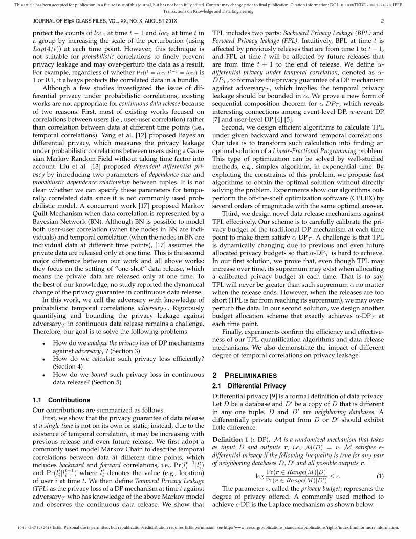
Example 5 (The supremum of BPL over time). Suppose thatMt satisfies ε-DP at each time point. In Figure 5, it shows themaximum BPL w.r.t. different ε and different transition matricesof PBi . In (a) and (b), the supremum does not exist. In (c) and (d),we can calculate the supremum using Theorem 11. The results arein line with the ones from computing BPL step by step at eachtime point using Algorithm 1.

Algorithm 6 for finding supreme of BPL or FPL is correctbecause, according to Theorem 8, all possible q and d thatgive the maximum value in Equation (24) are in the matricesqM and dM . Algorithm 6 is useful not only for designingprivacy budget allocation strategies in this section, but also




Algorithm 6: Find Supermum of BPL or FPL.Input: εt ; qM; dM.Output: the supremum of BPL or FPL over time, q, d

1 sup = 0; q = 0; d = 02 foreach qc ∈ qM, dc ∈dM do3 Calculate a candidate supc using Theorem 11 ;4 if sup < supc then sup = supc; q = qc; d = dc

5 return sup, q, d

for setting an appropriate parameter am as the input ofAlgorithm 4 because we will show in experiments that alarger am makes Algorithm 4 time-consuming (while, toosmall am may result in failing to calculate privacy leakagefrom L(α) if the input α may be larger than am).

Achieving α-DPT by limiting upper bound. We nowdesign a privacy budget allocation strategy utilizing Theo-rem 11 to bound TPL. Theorem 11 tells us that, if it is not thestrongest temporal correlation (i.e., d = 0 and q = 1), we maybound BPL or FPL within a desired value by allocating anappropriate privacy budget to a traditional DP mechanismat each time point. In other words, we want a constant εtthat guarantee the supremum of TPL, which is equal to thesum of the supremum of BPL and the supremum of BPLsubtracting εt by Equation (11), will not larger than α. Basedon this idea, we design Algorithm 7 for solving such εt.

Algorithm 7: Achieving α-DPT by upper boundInput: PBi and PFi ; α (desired privacy level).Output: Privacy budgets εt satisfying α-DPT at each t

1 Find qMB , dMB using Algorithm 4 with PBi ;2 Find qMF , dMF using Algorithm 4 with PFi ;3 bingo = false; range = α; e = 0.5 ∗ α;4 do //binary search.5 range = 0.5 ∗ range;6 Calculate supB by Algorithm 6 with e and qMB , dMB ;7 Calculate supF by Algorithm 6 with e and qMF , dMF ;8 if supB + supF − e = α then bingo = true9 else if supB + supF − e > α then e = e− range

10 else e = e+ range11 while bingo = false12 return εt = e

Achieving α-DPT by privacy leakage quantification.Algorithm 7 allocates privacy budgets in a conservativeway: when T is short, the privacy leakage may not beincreased to the supremum. We now design Algorithm 8to overcome this drawback. Observing the supremum ofbackward privacy loss in Figure 5(c)(d), BPL at the first timepoint is much less than the supremum. Similarly, it is easy tosee that FPL at the last time point is much less than its supre-mum. Hence, we attempt to allocate more privacy budgetstoM1 andMT so that the temporal privacy leakage at everytime points are exactly equal to the desired level. Specifically,if we want that BPL at two consecutive time points areexactly the same value αB , i.e., BPL(Mt) = BPL(Mt+1) = αB ,we can derive that εt = εt+1 for t ≥ 2 (it is true for t = 1 onlywhen LB(·) = 0). Applying the same logic to FPL, we have anew strategy for allocating privacy budgets: assigning largerprivacy budgets at time points 1 and T , and constant valuesat time [2, T ] to make sure that BPL at time points [1, T − 1]are the same, denoted by αB , and FPL at time [2, T ] are thesame, denoted by αF . Hence, we have ε1 = αB and εT = αF .Let the value of privacy budget at [2, T ] be εm. We have (i)LB(αB)+εm = αB , (ii) LF (αF )+εm = αF and (iii) αB+αF−εm = α.Combing (i) and (iii), we have Equation (26); Combing (ii)and (iii), we have Equation (27).

LB(αB) + αF = α (26)

LF (αF ) + αB = α (27)

Based on the above idea, we design Algorithm 8 to solveαB and αF . Since αB should be in [0, α], we heuristicallyinitialize αB with 0.5 ∗ α in Line 3 and then use binarysearch to find appropriate αB and αF that satisfy Equations(26) and (27).

Algorithm 8: Achieving α-DPT by quantificationInput: PBi and PFi ; α (desired privacy level for user i).Output: Privacy budgets εt, t ∈ [1, T ] satisfying α-DPT at each t

1 Find qMB , dMB , aMB using Algorithm 4 with PBi ;2 Find qMF , dMF , aMF using Algorithm 4 with PFi ;3 bingo = false; range = α; aB = 0.5 ∗ α;4 do //binary search.5 range = 0.5 ∗ range ;6 Find LB by Algorithm 5 with aB , qMB , dMB , aMB , ε = 0;7 aF = α− LB ; //Equation (26).8 Find LF by Algorithm 5 with aF with qMF , dMF , aMF , ε = 0;9 if LF + aB = α then bingo = true

10 else if LF + aB < α then aB = aB + range //Equation (27).11 else aB = aB − range12 while bingo = false

13 return ε1 = aB ; εt = aB + aF − α, t ∈ [2, T − 1]; εT = aF

6 EXPERIMENTAL EVALUATION

In this section, we design experiments for the following: (1)verifying the runtime and correctness of our privacy leakagequantification algorithms, (2) investigating the impact of thetemporal correlations on privacy leakage and (3) evaluatingthe data release Algorithms 7 and 8. We implemented all thealgorithms4 in Matlab2017b and conducted the experimentson a machine with an Intel Core i7 2.6 GHz CPU and 16GRAM running macOS High Sierra.

6.1 Runtime of Privacy Quantification AlgorithmsIn this section, we compare the runtime of our algorithmswith IBM ILOG CPLEX5, which is a well-known softwarefor solving optimization problems, e.g., the linear-fractionalprogramming problem (19)∼(21) in our setting.

For verifying the correctness of three privacy quantifyingalgorithms, Algorithm 1, Algorithm 3 and Algorithm 5, wegenerate 100 random transition matrices with dimensionsize n = 30 and comparing the calculation results with theone solving LFP problem using CPLEX. We verified that allresults obtained from our algorithms are identical to the oneusing CPLEX w.r.t. the same transition matrix.

For testing the runtime of our algorithms, we run them30 times with randomly generated transition matrices, andrun CPLEX one time (because it is very time-consuming),and then calculate the average runtime for each of them.Since Algorithm 3 needs parameters that are precomputedby Algorithm 2, and Algorithm 5 needs L(·) that can beobtained using Algorithm 4, we also test the runtime ofthese precomputations. The results are shown in Figure 6.

Runtime vs. n. In Figures 6(a) and (b), we show theruntime of privacy quantification algorithms and precom-putation algorithms, respectively, In Figure 6(a), each algo-rithm takes inputs of α = 0.1 and n×n random probabilitymatrices. The runtime of all algorithms increase along with

4. Souce code: https://github.com/brahms2013/TPL5. http://www-01.ibm.com/software/commerce/optimization/cplex-

optimizer/. We use version 12.7.1.




100 200 300 400 500n (T=1,a=0.1)

10-10

10-5

100

105

1010

runt

ime

(sec

onds

)cplexAlgo1Algo3Algo5

(a) Quantification algorithms at one time (b) Pre-computation algorithms

27 hours

1 second

10-2 s

10-5 s

100 200 300 400 500n

0

20

40

60

80

runt

ime

(sec

onds

)

Algo2Algo4 (am=0.1)Algo4 (am=1)

(c) Quantification algorithms over T times

0.01 0.1 1 10 20 (n=10,T=1)

10-6

10-4

10-2

100

runt

ime

(sec

onds

)

Algo1Algo3Algo5

(d) Quantification algorithms at one time

2 3 5 10 30 50 100 300 100010-2

10-1

100

101

102

runt

ime

(sec

onds

)

Algo1Algo3 with Algo2Algo5 with Algo2&Algo4

Fig. 6. Runtime of Temporal Privacy Leakage Quantification Algorithms.

n because the number of variables in our LFP problemis n. The proposed Algorithms 1, 3 and 5 significantlyoutperform CPLEX. In Figure 6(b), we test precomputationprocedures. We observed that all algorithms are increasingwith n, but Algorithm 4 is more susceptible to am. Algo-rithm 4 with a larger am results in higher runtime becauseit performs binary search in [0, am].

These results are in line with our complexity analysis,which shows the complexity of Algorithms 2 and 4 are O(n3)

and O(n2 logn+m logm) (m is the amount of transition pointsand increasing with am), respectively. However, when n oram is larger, pre-computation Algorithms 2 and 4 are time-consuming because we need to find optimal solutions forn∗(n−1) LFP problems given a n-dimension transition ma-trix. This can be improved by advanced computation toolssuch as parallel computing because here each LFP problemis independently solved, and such computation only needsto be run one time before starting to release private data.Another interesting way to improve the runtime is to findthe relationship between the optimal solutions of differentLFP problems given a transition matrix (so that we canprune some computations). We defer this to future study.

Runtime vs. T . In Figure 6(c), we test the runtime ofeach privacy quantification algorithm integrated with theirprecomputations over different length of time points. Wewant to know how can we benefit from these precompu-tations over time. All algorithms take inputs of 100 × 100matrices and εt = 0.1 for each time point t. The parametersof Algorithm 4 need to be initialized by Algorithm 2, so wetake them as an integrated module along with Algorithm 5.It shows that, Algorithm 1 runs fast if T is small. Algorithm3 becomes the most preferable if T is in [5, 300]. However,when T is larger than 300, Algorithm 5 with its precom-putation (Algorithm 4 with am = (T + 1) ∗ εt which is theworst case of supremum) is the fast one and its runtime isalmost constant with the increase of T . Therefore, there isno best algorithm in efficiency without a known T , but wecan choose appropriate algorithm adaptively.

Runtime vs. α. In Figure 6(d), we show that, a largerprevious BPL (or the next FPL), i.e., α, may lead to higherruntime of Algorithm 1, whereas other algorithms are rel-atively stable for varying α. The reason is that, when α islarge, Algorithm 1 may take more time in Lines 9 and 10for updating each pair of qj ∈ q+ and dj ∈ d+ to satisfyInequality (22). An update in Line 10 is more likely to occurdue to a large α because q(eα−1)+1

d(eα−1)+1is increasing with α.

However, such growth of runtime along with α will not lastso long because the update happens n times in the worsecase. As shown in Figure 6(b), when α > 10, the runtime of

Algorithm 1 becomes stable.

6.2 Impact of Temporal Correlations on TPLIn this section, for the ease of exposition, we only present theimpact of temporal correlations on BPL because the growthof BPL and FPL are in the same way.

The setting of temporal correlations. To evaluate if ourprivacy loss quantification algorithms can perform well un-der different degrees of temporal correlations, we find a wayto generate the transition matrices to eliminate the effect ofdifferent correlation estimation algorithms or datasets. First,we generate a transition matrix indicating the “strongest”correlation that contains probability 1.0 in its diagonalcells (this type of transition matrix will lead to an upperbound of TPL). Then, we perform Laplacian smoothing [20]to uniformize the probabilities of Pi (the uniform transitionmatrix will lead to an low bound of TPL). Let pjk be anelement at the jth row and kth column of the matrix Pi. Theuniformized probabilities p̂jk are generated using Equation(28), where s is a positive parameter that controls thedegrees of uniformity of probabilities in each row. Hence,a smaller s means stronger temporal correlation. We notethat, different s are only comparable under the same n.

p̂jk =pjk + s∑n

u=1 (pju + s)(28)

We examined s values ranging from 0.005 to 1 and setn to 50 and 200. Let ε be the privacy budget ofMt at eachtime point. We test ε = 1 and 0.1. The results are shown inFigure 7 and are summarized as follows.

Privacy Leakage vs. s. Figure 7 shows that the privacyleakage caused by a non-trivial temporal correlation willincrease over time, and such growth first increases sharplyand then remains stable because it is gradually close toits supremum. The increase caused by a stronger temporalcorrelations (i.e., smaller s) is steeper, and the time for theincrease is longer. Consequently, stronger correlations resultin higher privacy leakage.

Privacy Leakage vs. ε. Comparing Figures 7(a) and(b), we found that 0.1-DP significantly delayed the growthof privacy leakage. Taking s = 0.005, for example, thenoticeable increase continues for almost 8 timestamps whenε = 1 (Figures 7(a)), whereas it continues for approximately80 timestamps when ε = 0.1 (Figures 7(b)). However, aftera sufficient long time, the privacy leakage in the case ofε = 0.1 is not substantially lower than that of ε = 1 understronger temporal correlations. This is because, although theprivacy leakage is eliminated at each time point by setting asmall privacy budget, the adversaries can eventually learnsufficient information from the continuous releases.

Privacy Leakage vs. n. Under the same s, TPL is smallerwhen n (dimension of the transition matrix) is larger, as




Fig. 7. Evaluation of BPL under different degrees of correlations.

0 10 20 30

time

0

0.2

0.4

0.6

0.8

1

priva

cy lo

ss

0 10 20 30

time

0

0.2

0.4

0.6

0.8

1

priva

cy lo

ss

Allocated Budgets BPL FPL TPL

(a) Algorithm 7 (b) Algorithm 8

Fig. 8. Privacy Budget Allocation Schemes for 1-DPT .

shown in the lines s = 0.005 with n = 50 and n = 200 ofFigure 7. This is because the transition matrices tend to beuniform (weaker correlations) when the dimension is larger.

6.3 Evaluation of Data Releasing AlgorithmsIn this section, we first show a visualization of privacyallocation of Algorithms 7 and 8, then we compare the datautility in terms of Laplace noise.

Figure 8 shows an example of budget allocation, w.r.t.PBi =

(0.8 0.20.2 0.8

) and PFi =(

0.8 0.20.1 0.9

). The goal is 1-DPT . It iseasy to see that Algorithm 8 has better data utility becauseit exactly achieves the desired privacy level.

Figure 9 shows the data utility of Algorithms 7 and 8with 2-DPT . We calculate the absolute value of the Laplacenoise with the allocated budgets (as shown in Figure 8).Higher value of noise indicates lower data utility. In Figure9(a), we test the data utility under backward and forwardtemporal correlation both with parameter s = 0.001, whichmeans relatively strong correlation. It shows that, when Tis short, Algorithm 8 outperforms Algorithm 7. In Figure9(b), we investigate the data utility under different degreeof correlations. The dash line indicates the absolute valueof Laplace noise if no temporal correlation exists (privacybudget is 2). It is easy to see that the data utility significantlydecays under strong correlation s = 0.01.

7 RELATED WORK

Dwork et al. first studied differential privacy under continualobservation and proposed event-level/user-level privacy [4][5]. A plethora of studies have been conducted to investigatedifferent problems in this setting, such as high dimensionaldata [1] [8], infinite sequence [7] [21] [22], and real-timepublishing [6] [23]. To the best of our knowledge, no studyhas reported the risk of differential privacy under temporalcorrelations for the continuous aggregate release setting.Although [14] have considered a similar adversarial modelin which the adversaries have prior knowledge of temporalcorrelations represented by Markov chains, they proposeda mechanism extending differential privacy for releasinga private location, whereas we focus on the scenario ofcontinuous aggregate release with DP.

Abso

lute

Val

ue o

f Lap

lace

Noi

se

0

8.75

17.5

26.25

35

5 10 50

Algorithm 7 Algorithm 8

Abso

lute

Val

ue o

f Lap

lace

Noi

se

0

1

2

3

4

0.01 0.1 1

Algorithm 7 Algorithm 8(a) n=50, s=0.001 (b) n=50, T=10

T (length of release time) s (degree of correlations)

Fig. 9. Data utility of 2-DPT mechanisms.

Several studies have questioned whether differential pri-vacy is valid for correlated data. Kifer and Machanavajjhala[24] [25] [16] first raised the important issue that differentialprivacy may not guarantee privacy if adversaries know thedata correlations between tuples. They [24] argued that it isnot possible to ensure any utility in addition to privacy with-out making assumptions about the data-generating distribu-tion and the background knowledge available to an adver-sary. To this end, they proposed a general and customizableprivacy framework called PufferFish [25] [16], in which thepotential secrets, discriminative pairs, and data generationneed to be explicitly defined. Song et al. [17] proposedMarkov Quilt Mechanism when the correlations can bemodeled by Bayesian Network. Yang et al. [12] investigateddifferential privacy on correlated tuples described using aproposed Gaussian correlation model. The privacy leakagew.r.t. adversaries with specified prior knowledge can beefficiently computed. Zhu et al. [26] proposed correlateddifferential privacy by defining the sensitivity of queries oncorrelated data. Liu et al. [13] proposed dependent differen-tial privacy by introducing dependence coefficients for ana-lyzing the sensitivity of different queries under probabilisticdependence between tuples. Most of the above works deadwith correlations between users in the database, i.e., user-user correlations, in the setting of one-shot data release,whereas we deal with the correlation among single user’sdata at different time points, i.e., temporal correlations, andfocusing on the dynamic change of privacy guarantee incontinuous data release.

On the other hand, it is still controversial [27] whatshould be the guarantee of DP on correlated data. Li etal. [27] proposed Personal Data Principle for clarifying theprivacy guarantee of DP on correlated data. It states thatan individual’s privacy is not violated if no data aboutthe individual is used. By doing this, one can ignore anycorrelation between this individual’s data and other users’data, i.e.,user-user correlations. On the other hand, thequestion of “what is individual’s data”, or “what shouldbe an appropriate notion of negiboring databases” is trickyin many application scenarios such as genomic data. If weapply Personal Data Principle to the setting of continuousdata release, event-level privacy is not a good fit for protect-ing individual’s privacy because a user’s data at each timepoint is only a part of his/her whole data in the streamingdatabase. Our work shares the same insight with PersonalData Principle on this point: we show that the privacyloss of event-level privacy may increase over time undertemporal correlation, while the guarantee of user-privacy isas expected. We note that, when the data stream is infiniteor the end of data release is unknown, we can only resortto event-level privacy or w-event privacy [7]. Our workprovides useful tools against TPL in such setting.




8 CONCLUSIONS

In this paper, we quantified the risk of differential privacyunder temporal correlations by formalizing, analyzing andcalculating the privacy loss against adversaries who haveknowledge of temporal correlations. Our analysis showsthe privacy loss of event-level privacy may increase overtime, while the privacy guarantee of user-level privacyis as expected. We design fast algorithms for quantifyingtemporal privacy leakage which enables private data releasein real-time. This work opens up interesting future researchdirections, such as investigating the privacy leakage undertemporal correlations combining with other type of corre-lation models, and use our methods to enhance previousstudies that neglected the effect of temporal correlations incontinuous data release.

ACKNOWLEDGMENTS

This work was supported by JSPS KAKENHI Grant Number16K12437, 17H06099, JSPS Core-to-Core Program, A. Ad-vanced Research Network, the National Institute of Health(NIH) under award number R01GM114612, the Patient-Centered Outcomes Research Institute (PCORI) under con-tract ME-1310-07058, and the National Science Foundationunder award CNS-1618932.

REFERENCES

[1] G. Acs and C. Castelluccia, “A case study: Privacy preservingrelease of spatio-temporal density in paris,” in KDD, 2014, pp.1679–1688.

[2] J. Bolot, N. Fawaz, S. Muthukrishnan, A. Nikolov, and N. Taft,“Private decayed predicate sums on streams,” in ICDT, 2013, pp.284–295.

[3] T.-H. H. Chan, E. Shi, and D. Song, “Private and continual releaseof statistics,” ACM Trans. Inf. Syst. Secur., vol. 14, no. 3, pp. 26:1–26:24, 2011.

[4] C. Dwork, “Differential privacy in new settings.” in SODA, 2010,pp. 174–183.

[5] C. Dwork, M. Naor, T. Pitassi, and G. N. Rothblum, “Differentialprivacy under continual observation,” in STOC, 2010, pp. 715–724.

[6] L. Fan, L. Xiong, and V. Sunderam, “FAST: differentially privatereal-time aggregate monitor with filtering and adaptive sam-pling,” in SIGMOD, 2013, pp. 1065–1068.

[7] G. Kellaris, S. Papadopoulos, X. Xiao, and D. Papadias, “Differ-entially private event sequences over infinite streams,” PVLDB,vol. 7, no. 12, pp. 1155–1166, 2014.

[8] Y. Xiao, L. Xiong, L. Fan, S. Goryczka, and H. Li, “DPCube:differentially private histogram release through multidimensionalpartitioning,” Trans. Data Privacy, vol. 7, no. 3, pp. 195–222, 2014.

[9] C. Dwork, “Differential privacy,” in ICALP, 2006, pp. 1–12.[10] C. Dwork, F. McSherry, K. Nissim, and A. Smith, “Calibrating

noise to sensitivity in private data analysis,” in TCC, 2006, pp.265–284.

[11] R. Chen, B. C. Fung, P. S. Yu, and B. C. Desai, “Correlated networkdata publication via differential privacy,” VLDBJ, vol. 23, no. 4, pp.653–676, 2014.

[12] B. Yang, I. Sato, and H. Nakagawa, “Bayesian differential privacyon correlated data,” in SIGMOD, 2015, pp. 747–762.

[13] Changchang Liu, Supriyo Chakraborty, and Prateek Mittal, “De-pendence makes you vulnerable: Differential privacy under de-pendent tuples,” in NDSS, 2016.

[14] Y. Xiao and L. Xiong, “Protecting locations with differential pri-vacy under temporal correlations,” in CCS, 2015, pp. 1298–1309.

[15] F. D. McSherry, “Privacy integrated queries: an extensible platformfor privacy-preserving data analysis,” in SIGMOD, 2009, pp. 19–30.

[16] D. Kifer and A. Machanavajjhala, “Pufferfish: A framework formathematical privacy definitions,” ACM Trans. Database Syst.,vol. 39, no. 1, pp. 3:1–3:36, 2014.

[17] S. Song, Y. Wang, and K. Chaudhuri, “Pufferfish privacy mecha-nisms for correlated data,” in SIGMOD, 2017, pp. 1291–1306.

[18] Z. Jorgensen, T. Yu, and G. Cormode, “Conservative or liberal?personalized differential privacy,” in ICDE, 2015, pp. 1023–1034.

[19] E. B. Bajalinov, Linear-Fractional Programming Theory, Methods, Ap-plications and Software, 2003, vol. 84.

[20] O. Sorkine, D. Cohen-Or, Y. Lipman, M. Alexa, C. Rössl, and H.-P.Seidel, “Laplacian surface editing,” in SGP, 2004, pp. 175–184.

[21] Y. Cao and M. Yoshikawa, “Differentially private real-time datarelease over infinite trajectory streams,” in MDM, vol. 2, 2015, pp.68–73.

[22] ——, “Differentially private real-time data publishing over infinitetrajectory streams,” IEICE Trans. Inf.& Syst., vol. E99-D, no. 1, pp.163–175, 2016.

[23] H. Li, L. Xiong, X. Jiang, and J. Liu, “Differentially private his-togram publication for dynamic datasets: An adaptive samplingapproach,” in CIKM, 2015, pp. 1001–1010.

[24] D. Kifer and A. Machanavajjhala, “No free lunch in data privacy,”in SIGMOD, 2011, pp. 193–204.

[25] ——, “A rigorous and customizable framework for privacy,” inPODS, 2012, pp. 77–88.

[26] T. Zhu, P. Xiong, G. Li, and W. Zhou, “Correlated differentialprivacy: Hiding information in non-IID data set,” IEEE Trans.Inf.Forensics Security., vol. 10, no. 2, pp. 229–242, 2015.

[27] N. Li, M. Lyu, D. Su, and W. Yang, “Differential privacy: Fromtheory to practice,” in Synthesis Lectures on Information Security,Privacy, Trust, 2016, pp. 1–138.

[28] W. Dinkelbach, “On nonlinear fractional programming,” Manage-ment Science, vol. 13, no. 7, pp. 492–498, 1967.

Yang Cao received B.S. degree from the Schoolof Software Engineering, Northwestern Poly-technical University, China, in 2008, the M.S.degree and Ph.D. degree from the GraduateSchool of Informatics, Kyoto University, Japan,in 2014 and 2017, respectively. He is currentlya Postdoctoral Fellow at the department of Mathand Computer Science, Emory University, USA.His research interests are privacy preservingdata publishing and mining.

Masatoshi Yoshikawa received the B.E., M.E.and Ph.D. degrees from Department of Infor-mation Science, Kyoto University in 1980, 1982and 1985, respectively. Before joining GraduateSchool of Informatics, Kyoto University as a pro-fessor in 2006, he has been a faculty member ofKyoto Sangyo University, Nara Institute of Sci-ence and Technology, and Nagoya University.His general research interests are in the areaof databases. His current research interests in-clude multi-user routing algorithms and services,

theory and practice of privacy protection, and medical data mining. Heis a member of ACM and IPSJ.

Yonghui Xiao received 3 B.S. degrees fromXi’an Jiaotong University, China, in 2005. Heobtained the M.S. degree from Tsinghua Univer-sity in 2011 after spending two years working inindustry. He obtained the Ph.D. degree in thedepartment of Math and Computer Science atEmory University in 2017. He is currently a soft-ware engineer at Google.

Li Xiong is a Winship Distinguished ResearchProfessor of Computer Science (and BiomedicalInformatics) at Emory University. She holds aPhD from Georgia Institute of Technology, anMS from Johns Hopkins University, and a BSfrom University of Science and Technology ofChina, all in Computer Science. She and herresearch group, Assured Information Manage-ment and Sharing (AIMS), conduct research thataddresses both fundamental and applied ques-tions at the interface of data privacy and security,

spatiotemporal data management, and health informatics.

Documents

ATEX CLASS FILES, VOL. XX, NO. X, AUGUST 201X 1