TRANSPORTATION RESEARCH RECORD 1105 41

At-Rest to Active Earth Pressure Transition

S. BANG AND H. T. KIM

An approximate analytical procedure Is described to estimate the developed lateral earth pressures behind a rigid retaining waJJ experiencing outward tilt about the base with horizontal coheslonless backfill soil. Included are various stages of waJI tilt, starting from an at-rest condltlon to a full-active condition. The at-rest condition is defined as a stage of no-waJI tilt, whereas the full-active condition occurs when the soil elements along the entire depth or the wall are In an active state. The predictions from tlte developed method of analysis are com­pared with model test measurements. Tbe comparisons show very good agreement at various stages or retaining wall tilt. Finally, examples are provided to Illus trate the transition of the lateral earth pressures behind a smootl1 and a rough retaining wall.

Estimation of the lateral earth pressure development has been one of the most important aspects in geotechnical engineering practice (1-4) because it governs the design of many engineer­ing structures, including the retaining walls. Retaining walls are typically designed based on the active lateral earth pres­sures due to the tendency of outward tilt about the base. Classical lateral earth pressure theories, for example, Cou­lomb's and Rankine's (5), have been widely used for this purpose.

Because a certain amount of strain must develop within the backfill soil mass in order that the shear stresses that help to support the soil mass may be fully mobilized, a certain amount of wall tilt must be allowed before the lateral earth pressure reduces to the value of the active lateral earth pressure (6). However, when the movement of the wall is restricted or less than the magnitude necessary for the development of active condition, the developed lateral earth pressures could be greater than the active lateral earth pressures. Numerous such instances have been reported, indicating that the lateral earth pressure distribution behind the retaining structures must be associated not only with the type of structural movement taking place but also with the magnitude of the movement developed.

Described in this paper is a method of estimating the magni­tude and distribution of the lateral earth pressure exerted by horizontal cohesionless backfill soil behind a vertical rigid retaining wall experiencing outward tilt about its base from an "at-rest" condition to an "initial-active" condition to a "full­active" condition. The description of an at-rest condition fol­lows the conventional description, that is, the state of no-wall movement. The initial active condition refers to a stage of wall tilt when only the soil element at the ground surface experi­ences a sufficient lateral movement (limiting deformation) to achieve an active state defined by a Mohr-Coulomb stress relationship (5). The full-active condition occurs when the entire zone of soil elements from the ground surface to the base of the wall are in an active state; that is, stresses are in a

Department of Civil Engineering, South Dakota School of Mines and Technology, Rapid City, S.D. 57701-3995.

limiting condition at this stage. Between the at-rest and full­active conditions, "intermediate-active" conditions exist. The transition of the lateral earth pressures from an at-rest to a full active condition is discussed and the developed method of analysis is used to compare with the model test results. Finally, examples are presented to illustrate the transition of the lateral earth pressures.

FORMULATION

Stress equilibrium in two-dimensional plane strain state (7) can be written as

(la)

(lb)

where the coordinate x is measured positive from the top of the retaining wall toward the backfill and the coordinate z is mea­sured positive from the top of the retaining wall toward the base; y indicates the unit weight of the soil.

Because Equations la and lb include three unknowns, ax• Oz, and 'txv an addi1ional equation needs to be introduced. Here the third equation assumes the relationship between the major and minor principal stresses, that is,

a 3 = a 1[(1 - simv)/(l + sin'!')] (2)

Figure 1 shows the schematic representation of Equation 2. Note that if 'I' equals I)>, where I)> represents the internal friction angle of the cohesionless soil, then Equation 2 reduces to conventional Rankine's lateral earth pressure expression

a 3 = a 1[(1 - sinl)>)/(l + sinl)>)] = cr1 tan2 [(1t/4 - l)>/2)] (3)

Solution of Equations la and lb in conjunction with Equation 3

T

0

a

FIGURE 1 Stress relationship.

42

and boundary conditions will produce stress conditions at the limiting state, that is, full-active condition. This has already been solved by Sokolovskii in 1956 (8).

To describe the transition of lateral earth pressures from at­rest to initial-active to full-active condition, Equation 3 has been modified. When the retaining wall is in an at-rest condi­tion, no shear stress along the wall develops. Therefore in general

(4)

where K0 indicates the at-rest lateral earth pressure coefficient. IfK0 is known, the corresponding angle relating cr3 and cr1, 11>0 ,

can be easily obtained

sin<l>0 = (1 - K 0 )/(l + K~ (5)

Equation 4 then becomes

(6)

If Jaky's equation (9), K 0 = 1 - sinl!>, is used, then

sin<l>0 = sin<l>/(2 - sin<l>) (7)

By varying the angle, 'ljf, which describes the relationship between the major and minor principal stresses, from 1!>0 to<!>, Equation 2 may represent both Equations 3 and 6, that is, from an at-rest to a full-active condition. Furthermore, the rotation of the wall about its base may produce different stress ratios at various depths depending on the stage of the wall tilt, for example, a portion of the soil whose deformation exceeds the limiting value may achieve 'ljf = <l> state, whereas the remaining portion may still have <l>o < 'If < 11>. Therefore, 'If may be described as a function of the depth, that is, 'I'= 'ljf(z). Note that in reality 'ljf may be a function of both x and z. However, the effect of x coordinate has been neglected for the purpose of obtaining an approximate solution. In other words, the physical model describing the function 'ljf(z) can be visualized from a soil mass composed of an infinite number of infinitesimally thin horizontal layers with frictionless interfaces. Based on this assumption, Equations la and lb and 2 can be rewritten.

Define; at any depth, z

(8)

and 0 = rotation angle from x-axis to the direction of the major principal stress, o 1. These are indicated in Figure 1. The stresses can then be expressed as

ox = CJ (1 + sin'ljf(z) cos20) (9a)

O"z = CJ (1 - sin'ljf(z) cos20) (9b)

'txz = CJ sin'ljf(z) sin20 (9c)

TRANSPORTATION RESEARCH RECORD 1105

Substitution of Equations 9a, 9b, and 9c into Equations la and lb yields

acr/ax [1 + sin'ljf(z) cos20] + (oCJ/oz) sin'ljf(z) sin20

- 2cr sin'ljf(z) [sin20 ('00/ox) - (1/2) sin20/tan'lf(z)

o'lf(z)/oz - cos20 ('00/oz)] = o (10)

dCJ/ox [sin'ljf(z)sin20] + o<J/07. [1 - sim11(z)cos20]

+ 2cr sin'lf(z)[cos20 ('00/ox) - (1/2) cos20/tan'lf(z)

o'lf(z)/oz + sin20 ('00/oz)] = 'Y (11)

The Point A in Figure 1 indicates an orientation of the plane, which satisfies CJn tan'lf(z) = 'tn. The rotation angle, µ, from the direction of cr1 to this "pseudo-slip" plane therefore becomes

µ = [1t/4 - 'lf(Z)/2] (12)

as schematically shown in Figure 2. Therefore the slope of the pseudo-slip line, dz/dx, becomes

dz/dx = tan(0±µ) (13)

Multiplying Equation 10 by [sin (0±µ)/cos'lf(z)], Equation 11 by - [cos(0±µ)/cos'lf(Z)] and adding can yield

[oCJ/ox + 2crtan'lf(Z) a01ax ± ytan'ljf(z) ± CJ O'ljf(Z)/oz]

cos (0+µ) + [oo/oz + 2crtan'ljf(z) d0/oz - y]

sin (0+µ) = 0 (14)

Multiplying Equation 14 by [dx/cos (0±µ)] and using Equa­tion 13, the following expressions are obtained

dcr - 2otan'lf(z)d0 = y[dz - tan'lf(z)dx]

- o [o'ljf(z)/dz] dx

dcr + 2otan'ljf(z)d0 = "/[dz + tan'ljf(z)dx]

+ CJ [o'ljf(z)/dz] dx

(15)

(16)

Equations 13, 15, and 16 can be solved simultaneously for o and 0 at various coordinate points, which in tum can be used

I , 8

z FIGURE 2 Orientation of pseudo-slip lines.

x

BANG AND KIM

for the detailed calculation of the developed lateral earth pres­sures.

SOLUTION STEPS

Equations 13, 15, and 16 can be rewritten in different forms as

7.· · - Z· 1 · = (X· · - Y· 1 ·) tan(9· 1 · - ti. 1 ·) •J 1- J lJ ··- J 1- ,J ri- J (17)

7 .. · - Z· · 1 = (X· · - X· · 1) tan(9 .. 1 + µ. · 1) •J lJ- lJ lJ- lJ- lJ- (18)

(crij - <Ji-1} - 2 oi-1,J (9ij - ei-lj) tan'l'i-lj = 'Y[(z. · - z. 1 ·) - (x· · - X· 1 ·) tan'ljl· 1 ·] lJ 1- J lJ 1- J 1- J

- 0· 1 · (X· · - X· 1 ·) C)\jf'C)z 1. 1 · 1- J lJ 1- J ,, 1- J (19)

(oij - oij-1) + 2 oij-1 (9ij - 9ij-1) tan'l'ij-1 = 'Y[(z. · - z. · 1) + (x· · - X· · 1) tan'ljl· · 1] 1J lJ- lJ lJ- lJ-

+ O·. 1 (x·. - X·. 1) a'"'ozl .. 1 lJ- lJ lJ- Tl' IJ- (20)

These equations completely described recursion formulas for lhe pseudo-slip line coordinates (Xjj and ~j), the pseudo-slip line slope (01j±µi)• and Lhe associated average stress (oiJ) in terms of previous values at coordinates (i-1,j) and (iJ-1). According to Sokolovskii (8), the pseudo-slip lines form in general in three distinct regions as shown in Figure 3. The solution process starts from the line, 01A0 , that is, the ground surface whose coordinates and stress values are known, to the Hoe OzA3, that is, the rear face of the retaining wall through Regions I, II, and III. The detailed description of the solution procedure is beyond the scope of this paper; it is well described by Sokolovskii (8).

Along the free surface 01A0 , all values are known as

(21)

A,

x

II

A, O, ....._- -----1A,

Ill

z A,

Psuedo·Sllp Line Envelope Solution Domain

FIGURE 3 Schematics of solution procedure.

43

This leads to the complete solution of Xi_j• zij• aij• and 9ij in Region I. For the solution of Region Il, values of oij• 9ij• xij• and zij along 0102 are needed in addition to those values along 01A1 obtained from the solution of Region I. Obviously at 01 or 02 (actually some point but separated conveniently for the solution), Oij = 0, xij = 0, and ~j = 0. However, 91j varies from rc/2 at 01 to some value at Oz where the wall friction may be considered. When the wall friction is considered, 9 can be expressed, according to Sokolovskii (8), as

9 = rc/2 + 1/2 (.1 - o) (22)

where o is the wall friction angle, and

sin.1 = sino/sin4> (23)

Because angle 'ljl(z) is introduced instead of <\>, Equation 22 is also modified as

9 = rc/2 + 1/2 [.1(z) - o(z)] (24)

where o(z) is the developed wall friction angle at depth z, and

sin .1(z) = [sino(z)/sin\jf(z)] (25)

and o(z) varies from zero at at-rest state to omax at active state with its variation in accordance with that of \jf(z). The values of 9ij along 010z, therefore, can be taken as

00 = rc/2 1

0oz = rc12 + 112 l.1(z) - o(z)l I z=0 (26)

with linear variation between 01 and Oz. This leads to the complete solution of Region II.

The solution of Region III requires at least two sets of initial values along OzA3 in addition to solutions along OzA2 obtained in Region II. Known initial values along 02A3 are

xij = 0

9ij = rc/2 + 1/2 [.1(z) - o(z)] I Z=Z· . lJ

(27)

Therefore a complete solution can be made possible. Once the values of oij along 02A3, that is, alon_g the rear face of the retaining wall, are obtained, developed normal and shear stresses can be calculated from

Ox = oi J' (sin [.1(z) - o(z)]/sin .1(z)} cos o(z) I z=z .. . ~

'txz = ox tan o(z) I Z=Z· . lJ

(28)

The detailed solution steps, however, require a description of the function, 'ljl(z), and its derivative, which describe the transi­tion of lateral earth pressures from an at-rest to a full-active condition. As discussed before, the function varies from c\>0 at at-rest condition to c\>0 at full-active condition. The variation between these two extreme values is assumed as follows.

44

0 ljJ(Z)

{J=2

H

z FIGURE 4 Transition of 'lf(z) from $

0 to

Ill·

Let p denote the stage of wall tilt so that p = 0 for at-rest condition, p = 1.0 for initial active condition, and P = 2.0 for full-active condition. In other words, for the values of P between 0 and 1.0, transition from an at-rest to an initial-active condition is described. Suppose that the behavior of the soil is elasto-fully plastic as defined by the limiting deformation, the values of p between 0 and 1.0 describe elastic behavior of the soil because the limiting deformation of the soil does not develop yet. Therefore it is assumed that the developed defor­mation of the soil for 0 S P S 1 is directly proportional to p.

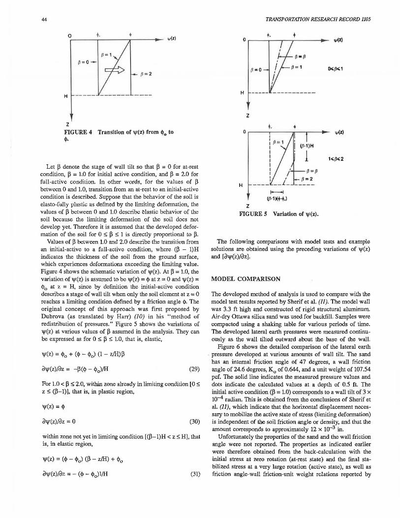
Values of P between 1.0 and 2.0 describe the transition from an initial-active to a full-active condition, where (p - l)H indicates the thickness of the soil from the ground surface, which experiences deformations exceeding the limiting value. Figure 4 shows the schematic variation of \jl(z). At P = 1.0, the variation of \jl(z) is assumed to be \jl(z) = Q> at z = 0 and \jl(z) = Q>0 at z = H, since by definition the initial-active condition describes a stage of wall tilt when only the soil element at z = 0 reaches a limiting condition defined by a friction angle $. The original concept of this approach was first proposed by Dubrova (as translated by Harr) (10) in his "method of redistribution of pressures." Figure 5 shows the variations of \jl(z) at various values of p assumed in the analysis. They can be expressed as for 0 S p S 1.0, that is, elastic,

'lf(Z) = $0 + ($ - Q>0 ) (1 - z/H)p

o\jl(z)/oz = -P(Q> - Q>J/H (29)

For 1.0 < p S 2.0, within zone already in limiting condition [OS z S (P-1)], that is, in plastic region,

\jl(z) = Q>

o\jl(z)/oz = o (30)

within zone not yet in limiting condition [ <P- l)H < z SH], that is, in elastic region,

\jl(z) = (Q> - <l>o) <P - z/H) + <l>o

o\jl(z)/Oz = - (Q> - Q>0 )1/H (31)

The following comparisons with model tests and example solutions are obtained using the preceding variations of \jl(z) and [o\jl(z)/oz].

MODEL COMPARISON

The developed method of analysis is used to compare with the model test results reported by Sherif et al. (11). The model wal.l was 3.3 ft high and constructed of rigid structural aluminum. Air-dry Ottawa silica sand was used for backfill. Samples were compacted using a shaking table for various periods of time. The developed lateral earth pressures were measured continu­ously as the wall tilted outward about the base of the wall.

Figure 6 shows the detailed comparison of the lateral earth pressure developed at various amounts of wall tilt. The sand has an internal friction angle of 47 degrees, a wall friction angle of 24.6 degrees, K

0 of 0.644, and a unit weight of 107 .54

pcf. The solid line indicates the measured pressure values and dots indicate the calculated values at a depth of 0.5 ft. The initial active condition <P = 1.0) corresponds to a wall tilt of 3 x 10-4 rm.lian. This is obtained from the conclusions of Sherif et al. (11), which indicate that the horizontal displacement neces­sary to mobilize the active state of stress (limiting deformation) is independent of the soil friction angle or density, and that the amount corresponds to approximately 12 x 10-3 in.

Unfortunately the properties of the sand and the wall friction angle were not reported. The properties as indicated earlier were therefore obtained from the back-calculation with the initial stress at zero rotation (at-rest state) and the final sta­bilized stress at a very large rotation (active state), as well as friction angle-wall friction-unit weight relations reported by

BANG AND KIM

; 40

"' (l=O. ,!;

! :I 30 "' {/)

! D.

.c 20 t: .. w ..

10 c 0 .!:! 0 ::c 0

0 2 4 6 8

Wall Rotation (x10-•rad)

FIGURE 6 Model test Comparison L

measured

• calculated

Sherif et al. (12). The comparison indicates that very good agreement exists between the measured and calculated lateral earth pressures in magnitude and variation at various degrees of wall tilt.

Sherif et al. (11) reported additional test results with the same model. Pressures were measured continuously at five different depths. Again, the detailed material properties were not indi­cated, therefore the same methods were used to obtain the material properties at corresponding depths of the measure­ments. The calculated soil friction angles vary from approx­imately 28 degrees at the lowermost pressure cell to approx­imately 46 degrees at the uppermost one. This wide variation in friction angle may raise a question. However, in the absence of direct measurements, these calculated friction angles could only be used for the comparison between experimental and analytical results. In the analysis, the soil is assumed to be composed of five layers whose material properties are repre­sented by the values calculated at the mid-depths. The detailed lateral earth pressure comparisons, as well as the material properties, are shown in Figure 7 and Table 1, respectively. As

Cii 200

fJ~ O . ,!; (J =0.3

! 160 (J =0.6 :I (J =0.9

"' (J= 1.2 {/) ID 120 (J=1 .5 ct (J=1.8

.c 80 t: -SPS ..

w SP4 iiii 40 SP3 c SP2 0 N SP1 "t: 0 0 ::c 0 5 10 15 20

Wall Rotation (x10-•rad)

-- me11ured 0 calculated

FIGURE 7 Model test Comparison 2.

45

TABLE I SAND PROPERTIES

Pressure Depth • Cell (ft) (deg) tano/tan«I> Ko

SPl 0.5 46 0.52 0.89 SP2 0.99 38 0.52 0.44 SP3 1.53 40 0.52 0.47 SP4 2.06 31 0.52 0.56 SP5 2.60 28 0.52 0.72

can be observed in the figure, the method of analysis can predict the developed lateral earth pressures at various depths and at various degrees of wall tilt closely, with the exception of pressure cell SP3 near ~ of 1.0--the measurement indicates a very sharp drop of earth pressures in contrast to the other pressure cell measurements.

EXAMPLE

The lateral earth pressures behind a vertical retaining wall experiencing outward tilt about its base with uniform cohesion­less backfill material are calculated at various values of ~. Figure 8 shows the results of a smooth (frictionless) retaining wall. From at-rest <P = 0) to initial-active condition (p = 1.0), lateral earth pressures decrease more rapidly with P near the middle portion of the wall, whereas rapid reduction in pressure is observed within the lower portion of the wall from an initial­active (~ = 1.0) to a full-active condition (p = 2.0). As expected,

-.c Q. ID c

2

4

6

H = 10 ft. + = 30' d =O'

k,=0.5 r=100 pct

8 Coulomb's

10 L-~...J.._~-'-~~.i.......;....__.._~_..~__,

0 100 200 300 400 500 600

Horizontal Lateral Earth Pressure (psi)

FIGURE 8 Transition of lateral earth pressures (smooth wall).

46

0

2

4

-.c a. ID 0

6

8

10

H = 10 II . + = 30° d = 16.1°

k. = 0.5 y = 100 pct

0 100 200 300 400 500 600

Horizontal Lateral Earth Pressure (psi)

FIGURE 9 Transltlon of lateral earth pressures (rough wall).

the magnitude and variation of the lateral earth pressure at full­active condition(~= 2.0) exactly matches Coulomb's solution because the slip lines are identical between two methods for a frictionless wall. For a rough retaining wall (Figure 9), however, the developed method of analysis does not match exactly Coulomb's solution because of the differences in the orientation of the slip lines; Coulomb's solution is still based on linear slip lines, whereas the developed method of analysis

0

2

4

-.c a. ID 0 6

8

20 40 60

H = 10 II.

+ = 30° d=16.1°

k,=0.5 r= 100 pct

80

Shear Stress (psi)

FIGURE 10 Transition of shear stresses.

100

TRANSPORTATION RESEARCH RECORD 1105

involves curved slip lines near the retaining wall. The dif­ference is very small, however.

Figure 10 shows the variations of the shear stresses behind the rough retaining wall from an at-rest to a full-active condi­tion. The variation begins with zero shear stresses at at-rest condition, and reaches maximum values at full-active condition with transitions in accordance with the values of ~. For instance, at~= 1.5, that is, when limiting condition reaches up to mid-depth, maximum possible shear stresses defined by the wall friction develop within the upper-half while the lower-half is yet to be within reach of full values.

CONCLUSIONS

An approximate analytical solution that describes the transition of the lateral earth pressures from an at-rest to a full-active condition behind a rigid retaining wall experiencing an outward tilt about the base has been developed. Comparisons with model test results have also been made. In general the developed method of analysis is capable of predicting not only the magnitudes but also the variations of the lateral earth pressures at various depths as well as at various amounts of wall tilt.

The developed analytical solution involves many assump­tions, including the at-rest earth pressure coefficient. For many earth-retaining structures, backfill materials may be placed by various methods, resulting in an initial stress state other than at­rest condition. In such cases the induced initial stress state could be represented in the analysis by appropriately express­ing the initial friction angle, q,0 , so that the resulting earth pressure ratio in Equation 6 represents the actual induced initial stress state.

The developed method of analysis can be easily expanded to include the cohesion of the soil, various geometry of the wall and the ground surface, and the depth-dependent soil strength characteristics, as well as other modes of wall movements. Further research is necessary, however, if other factors such as the large deformation effect, slippage between the structure and the soil, and the flexibility of the retaining structures are to be considered

REFERENCES

1. M. Fukuoka, T. Ak:atsu, S. Datagiri, T. lseda, A. Shimazu, and M Makagake. Earth Pressure Measurements on Retaining Walls. Proc., Nimh lnlernalional Conference on Soil Mechanics and Foundation Engineering, Tokyo, Japan, 1977.

2. I. K. Lee and J. R. Herington. Effect of Wall Movement on Active and Passive Pressures. Journal of the Soil Mechanics and Founda­tions Division, ASCE, Vol. 98, No. SM6, June 1972.

3. S. Okabe. General Theory of Earth Pressure. Journal of Japanese Society of Civil Engineers, Vol. 12, No. 1, 1924.

4. K. Terzaghi. General Wedge Theory of Earth Pressure. Transac­tion, ASCE, 1941.

5. T. W. Lambe and R. V. Whitman. Soil Mechanics, John Wiley and Sons, Inc., New York, 1969.

6. M. G. Spangler and R. L. Handy. Soil Engineering, 4th ed. Harper and Row, New York, 1982.

7. S. P. limoshenko and J. N. Goodier. Theory of Elasticity. 3rd ed. McGraw-Hill Book Co., New York, 1970.

TRANSPORTATION RESEARCH RECORD 1105

8. V. V. Sokolovskii. Statics of Granular Media. Pergamon Press, New York, 1965.

9. J. Jaky. The Coefficient of Earth Pressure at Rest Journal of the Society of Hungarian Architects and Engineers, 1944.

10. M. E. Harr. FoundaJions ofTheore,tical Soil Mechanics. McGraw­Hill Book Co., New York, 1966.

11. M. A. Sherif, Y. S. Pang, and R. I. Sherif. Ka and K0 Behind Rotating and Non-Yielding Walls. Journal of Geotechnical Engi­neering, Vol. 110, No. l, Jan. 1984.

47

12. M. A. Sherif, I. Ishibashi, and C. D. Lee. Dynamic Earth Pres­sures Against Retaining Structures. Soil Engineering Research Report 21, University of Washington, Seattle, Jan. 1981.

Publication of this paper sponsored by Committee on Subsurface Soil­Structure Interaction.

Initial Response of Foundations on Mixed Stratigraphies CHARLES E. WILLIAMS

A procedure for easily computing the Initial settlement of shallow foundations on mixed stratigraphies has been developed. Applicable soil conditions are primarily tiff to hard clays with horiwntal layers or dense to very dense sand. The Revised Gibson Model makes use of a simple equation for elastic settlement of axlsymmetrlc footings . An equivalent modulus that account for the variations In soil modulus with depth beneath the footing is one of tbe primary input param­eters to the equation. The effect of a sand layer within the foundation soils on initial settlements is Included in the pro· cedure by means of an additional factor obtained from para­metric charts. Twelve case histories, including elevated and ground storage tanks and multistory buildings, are used to evaluate the effectiveness of the new lnltlal settlement com­putational method.

The initial settlement component of the response of founda­tions to applied load is an important design consideration when the supporting soil media are comprised of stiff to hard clays. The presence of competent sand layers within the foundation stratum can effectively "stiffen" the foundation response and should be considered in design.

The Equivalent Gibson Model (1) has been shown to be a useful procedure for properly characterizing cohesive founda­tion media in the Houston, Texas, area and computing expected initial settlements for a large range of foundation sizes. The Equivalent Gibson Model has been expanded to consider the presence of competent sand layers within the supporting soils. The simplicity of the original procedure is maintained by

McBride-Ratcliff and Associates, Inc., 7220 Langtry, Houston, Texas 77040.

adding only one additional design step involving the use of parametric plots.

The new procedure was evaluated by application to 12 new projects ranging from elevated and ground storage tanks to multistory buildings. Measured initial settlements are com­pared with those predicted by the Revised Gibson procedure.

PREVIOUS WORK

Initial settlement represents the immediate foundation response to induced shear stresses at constant volume. The remaining two components of settlement due to consolidalion and second­ary compression involve time-related volume change. For stratigraphies containing moderately to heavily overconsoli­dated clays, the initial settlement component can account for 30 to 70 percent of the total settlement response (2). Consequently, the expected magnitude of initial settlement for foundations on soil strata with a large percentage of stiff to hard clay layers is a major design consideration. Development of the initial settle­ment component within the total response of a building founda­tion to applied load is shown in Figure 1.

Proper design of foundations typically results in contact pressures for footings or mats that do not produce yield zones in lhe foundation soils. The foundation response is to the left of the "first yield" location shown in Figure 2, which makes it possible to use elastic or linear methods of analysis Lo predict initial settlements.

Williams and Focht (1) recognized that Pleistocene clays in the Houston area typically exhibit an increase in undrained modulus with depth, and that the soil model proposed by