Asymptotic approximations of high frequency wave propagation problems

8/7/2019 Asymptotic approximations of high frequency wave propagation problems

http://slidepdf.com/reader/full/asymptotic-approximations-of-high-frequency-wave-propagation-problems 1/21

Asymptotic approximations of high frequency wave

propagation problems

Mohammad Motamed and Olof Runborg

Department of Numerical Analysis,

School of Computer Science and Communicatopm, KTH,

100 44 Stockholm

Sweden

Email: [email protected], [email protected]

Summary. The numerical simulation of highly oscillatory solutions of high frequency wavepropagation problems is important in many applications, including seismic, acoustic, optical

waves and microwaves. When the wavelength is short compared to the overall size of the

computational domain, and direct simulations using the standard wave equations are very ex-

pensive, due to requiring a large number of grid points to resolve the wave oscillations. There

are however computationally much less costly models, that are good approximations of many

wave equations and are used in applications. In this paper we consider asymptotic approx-

imations of high frequency waves. We focus on geometrical optics, geometrical theory of

diffraction and Gaussian beams and review the mathematical models and numerical methods

based on such asymptotic approximations.

1 Introduction

The numerical approximation of high frequency wave propagation is important in

many applications for different types of waves: elastic, electromagnetic as well as

acoustic. Examples include the forward and the inverse seismic wave propagation,

radiation and scattering problems in computational electromagnetics (CEM) and un-

derwater acoustics.

In this review we consider numerical simulation of waves at high frequencies and

the underlying mathematical models used. For simplicity we will mainly discuss the

linear scalar wave equation,

utt − c(x)2∆u = 0, (t,x) ∈ R+ × Ω, Ω ⊂ R

d, (1)

where c(x) is the local speed of wave propagation of the medium. We complement

(1) with initial or boundary data that generate high-frequency solutions. The ex-

act form of the data will not be important here, but a typical example would beu(0,x) = A(x) exp(iωk · x) where |k| = 1 and the frequency ω ≫ 1. With slight

modifications, the techniques we describe will also carry over to systems of wave

equations, like the Maxwell equations and the elastic wave equation.



2 Mohammad Motamed and Olof Runborg

When the frequency of the waves is high, (1) is a multiscale problem, where

the small scale is given by the wavelength, and the large scale corresponds to the

overall size of the computational domain. In the direct numerical simulation of (1)

the accuracy of the solution is determined by the number of grid points or elements

per wavelength. The computational cost to maintain constant accuracy grows alge-braically with the frequency, and for sufficiently high frequencies, direct numerical

simulation is no longer feasible. Numerical methods based on approximations of (1)

are needed.

Fortunately, there exist good approximations of many wave equations precisely

for very high frequency solutions. In this paper we consider variants of geometri-

cal optics (GO), which are asymptotic approximations obtained when the frequency

tends to infinity. Instead of the oscillating wave field the unknowns in standard ge-

ometrical optics are the phase and the amplitude, which typically vary on a much

coarser scale than the full solution. Hence, they should in principle be easier to com-

pute numerically.

The main drawbacks of the infinite frequency approximation of GO are that

diffraction effects at boundaries are lost, and that the approximation breaks downat caustics, where the predicted amplitude is unbounded. For these situations more

detailed models are needed, such as the geometrical theory of diffraction (GTD) [16],

which adds diffraction phenomena by explicitly taking into account the geometry of

Ω and boundary conditions. The solution’s asymptotic behavior close to caustics

can also be derived, and a correct amplitude for finite frequency can be computed

[21, 25, 13].

The purpose of this paper is to review the mathematical models and numerical

methods for high frequency waves based on GO and GTD. For other reviews of this

topic, see [3, 8, 24, 34]. The paper is organized as follows. In Section 2 the equations

used in GO are derived and a survey of numerical methods for such high frequency

models is given. The techniques to add diffraction effects and to correct the standard

geometrical optics approximation at caustics are discussed in Section 3.

2 Geometrical Optics

In this section, we first derive the equations that are used in geometrical optics. We

then review numerical methods based on different formulations.

2.1 Mathematical formulation

The starting point is the Cauchy problem for the scalar wave equation (1),

utt(t,x)

−c(x)2∆u(t,x) = 0, x

∈R

d, t > 0, (2)

u(0,x) = u0(x), x ∈ Rd,

ut(0,x) = u1(x), x ∈ Rd,



Asymptotic approximations of high frequency wave propagation problems 3

with highly oscillatory initial data u0 and u1. Here c(x) is the local wave velocity of

the medium. We also define the index of refraction as η(x) = c0/c(x) with the refer-

ence velocity c0 (e.g. the speed of light in vacuum). For simplicity we will henceforth

let c0 = 1. The wave equation (2) admits solutions of the type

u(t,x) = A(t,x, ω)eiωφ(t,x), (3)

with A and φ representing the amplitude and phase functions, respectively. The level

curves of φ corresponds to the wave fronts of a propagating wave.

Since (2) is linear, the superposition principle is valid and a sum of solutions is

itself a solution (provided initial data is adapted accordingly). The generic solution

to (2) is, at least locally, described by a finite sum of terms like (3),

u(t,x) =N

n=1

An(t,x, ω)eiωφn(t,x). (4)

with An, φn being smooth functions and An depending only mildly on the frequency

ω. Typically this setting only breaks down at a small set of points, namely focuspoints, caustics and discontinuities in c(x).

In this section, we will assume the geometrical optics approximation that ω →∞. This means that we accept the loss of diffraction phenomena in the solution and

the amplitude’s breakdown at caustics, which we will come back to in Section 3.

There are three strongly related formulations of geometrical optics, which we will

review here.

Eikonal equation

Let us start by deriving Eulerian PDEs for the phase and the amplitude functions that

are formally valid in the limit when ω → ∞. We consider time harmonic waves of

type u(t,x) = v(x)exp(iωt) with ω fixed. Inserting it into the time-dependentwaveequation (2), we get the Helmholtz equation

c2∆v + ω2v = 0. (5)

We assume that the solution to (2) has the form (3) and that thethe amplitude function

in (3) can be expanded in a power series in 1/iω. We then get the asymptotic WKB

expansion, [13],

v = eiωφ(x)∞

k=0

ak(x)(iω)−k (6)

and substitute it into (5). Equating coefficients of powers of ω to zero gives us the

eikonal equation and the the transport equation for the phase and the first amplitude

term in the frequency domain,

|∇φ| = 1/c = η, 2∇φ · ∇a0 + ∆φa0 = 0. (7)

For the remaining amplitude terms, we get additional transport equations




2∇φ · ∇ak+1 + ∆φak+1 + ∆ak = 0.

When ω is large, only the first term in the expansion (6) is significant, and the prob-

lem is reduced to computing the phase φ and the first amplitude term a0. Since the

family of curves x | φ(t,x) = φ(x) − t = 0, parametrized by t ≥ 0, describe apropagating wave front, we often directly interpret the frequency domain phase φ(x)as the travel time of a wave.

In what follows we will drop the tilde for the frequency domain quantities and

denote the first amplitude term a0 by A (or A1, A2, etc. when there are multiple

crossing waves).

One problem with the eikonal and transport equations is that they do not accept

solutions with multiple phases. There is no superposition principle for the nonlinear

eikonal equation. In fact, for the case in (4), the derivation must be done term wise,

and the φn and An will, locally, satisfy separate eikonal and transport equation

pairs. However, the eikonal equation still has a well-defined solution. It is a nonlinear

Hamilton–Jacobi-type equation with Hamiltonian H (x, p) = c(x)| p|. Extra condi-

tions are needed for this type of equations to have a unique solution known as theviscosity solution, which is the analogue of the entropy solution for hyperbolic con-

servation laws, [7]. As can be deduced from the previous paragraph, at points where

the correct solution should have a multivalued phase, i.e. be of the type in (4), the

viscosity solution picks out the phase corresponding to the first arriving wave, i.e.

the smallest φn in (4).

It is well known that solutions of Hamilton–Jacobi-equations can develop kinks,

i.e. discontinuities in the gradient, just as shocks appear in the solutions of conserva-

tion laws. In the case of the eikonal equation, the kinks are located where the physi-

cally correct phase solution should become multivalued. We notice that the transport

equation has a factor involving ∆φ, which is not bounded at kinks, and therefore we

can expect blow-up of a0 at these points.

Ray equations

Another formulation of geometrical optics is ray tracing, which gives the solution

via ODEs. This Lagrangian formulation is closely related to the method of char-

acteristics. Let (x(t), p(t)) be a bicharacteristic pair related to the Hamiltonian

H (x, p) = c(x)| p|. We are interested in solutions for which H ≡ 1. In this case

the projections on physical space, x(t), are usually called rays, and we have

dx

dt= ∇ pH (x, p) =

1

η2 p, x(0) = x0, (8)

d p

dt= −∇xH (x, p) =

∇η

η, p(0) = p0, | p0| = η(x0). (9)

Solving (8, 9) is called ray tracing. In d dimensions the bicharacteristics are curves

in 2d-dimensional phase space, (x, p) ∈ Rd×d. It follows that H is constant along

them, H (x(t), p(t)) = H (x0, p0). Note that p(t) ≡ ∇φ(x(t)) if p0 = ∇φ(x0).




Hence, with this initialization, the rays are always orthogonal to the level curves of

φ, since dx/dt is parallel to p = ∇φ by (8). Moreover, for our particular H ,

d

dtφ(x(t)) =

∇φ(x(t))

·dx(t)

dt= p(t)

· ∇ pH (x(t), p(t)) = H (x(t), p(t)) = 1.

Thus, as long as φ is smooth, we have

φ(x(t)) = φ(x0) + t.

Since φ corresponds to travel time, this also shows that the parametrization t in (8, 9)

actually corresponds to unscaled time; the ray x(t) traces one point on a propagating

wave front at time t. The absolute value of its time derivative |dx/dt| is precisely

the local speed of propagation c(x) by (8), and since p is parallel to dx/dt, while

| p| = H (x, p)c(x)−1 = c(x)−1, the vector p is often called the slowness vector.

As was discussed before, the solution of the eikonal equation is valid up to the

point where discontinuities appear in the gradient of φ. This is where the phase

should become multivalued but, by the construction, cannot. The bicharacteristics,

however, do not have this problem, and we can extend their validity to all t.

In order to compute the amplitude along a ray we also need information about

the local shape of the ray’s source. Let(x(t,x0), p(t,x0)) denote the bicharacteristic

originating in x0 with p(0,x0) = ∇φ(x0), hence x(0,x0) = x0. Let J (t,x0) be

the Jacobian of x with respect to initial data, J = Dx0x(t,x0), and assume that it is

nonsingular. The amplitude is then given by the expression, [26],

A(x(t,x0)) = A(x0)η(x0)

η(x(t,x0))

q(0,x0)

q(t,x0)

e−imπ

2 , (10)

where q = det J is the geometrical spreading measuring the size change of an in-

finitesimal area transported by the rays, and m = m(t) is a nonnegative integer called

the Keller–Maslov index. It represents the number of times q(·,x0) has changed signin the interval [0, t], i.e. the number of times that the ray has touched a caustic which

are sets of points where q = 0. These are points where rays concentrate, cf. Figure 5.

We see clearly from (10) that the amplitude is unbounded close to caustic points.

This formula is therefore valid only before and after these points.

The elements of the Jacobian is given by another ODE system, obtained by dif-

ferentiating (8, 9) with respect to x0,

d

dt

Dx0x

Dx0 p

=

D2

pxH D2 ppH

−D2xxH −(D2

pxH )T

Dx0x

Dx0 p

, (11)

with initial data

Dx0x(0,x0) = I, Dx0 p(0,x0) = D2φ(x0).

Here D2 represents the Hessian.

Note that since we have the constraint H (x, p) = 1, or | p| = η(x), the di-

mension of the phase space (x, p) can actually be reduced by one. For example in






utt − c(x)2∆u = 0

q

A c

Rays

d2xdτ

= 1

2∇η2

cRay tracing

d d d

©

Wave frontmethods

Kinetic

f t + 1

η2 p · ∇xf

+ 1

η∇xη · ∇pf = 0

cMoment methods,Full phase space

methods

Eikonal

|∇φ| = η

cHamilton–Jacobi

methods

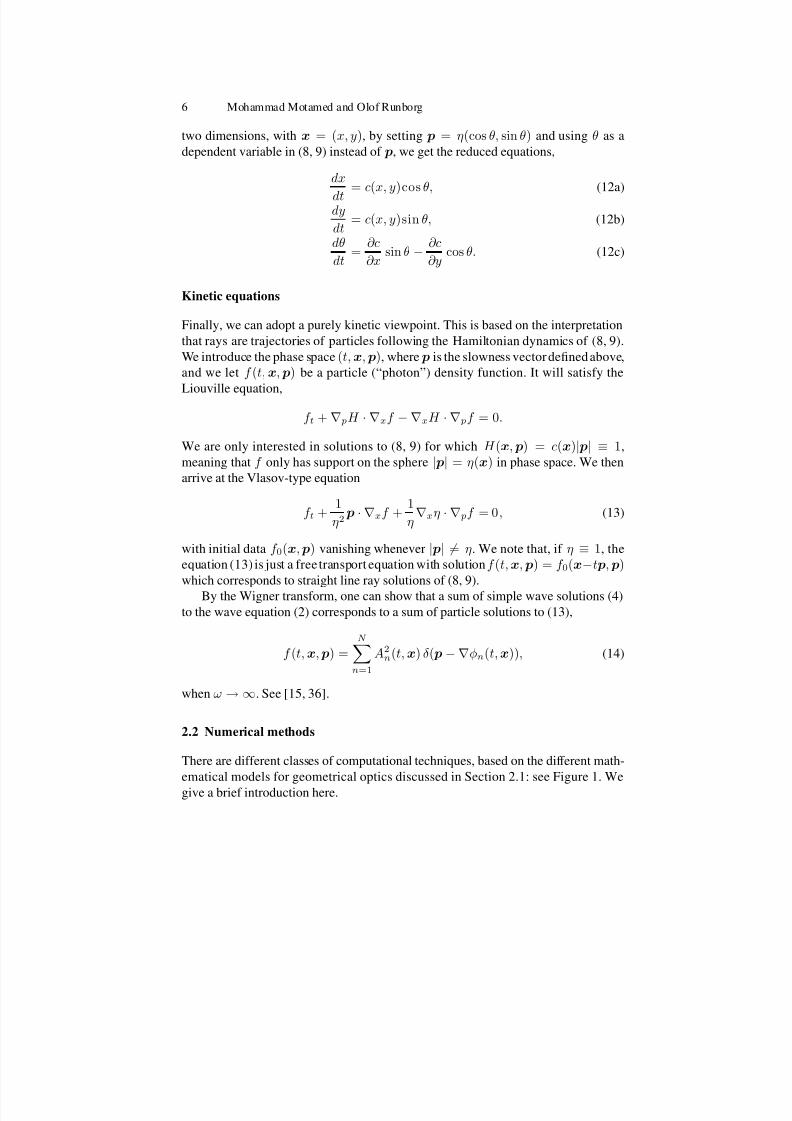
Fig. 1. Mathematical models and numerical methods. Wave front methods use aspects of both

the ray and the kinetic model.

Ray tracing

The ray equations derived in Section 2.1 are the basis for ray tracing. The ray x(t)and slowness vector p(t) = ∇φ(x(t)) are governed by the ODE system (8, 9). This

system together with another ODE system for the amplitude, (11), are solved with

standard ODE solvers giving the phase and amplitude along the ray. The solution at a

desired point is then interpolated from the solutions along the rays. This can be rather

difficult in the regions where ray tracing produces diverging or crossing rays. More-

over, ray tracing is only of interest for problems involving a few number of source

points. For problems with many source points, ray tracing may be computationally

expensive. Some general references on ray tracing are [6, 22].

Hamilton–Jacobi methods

To avoid the problem of diverging rays, several PDE-based methods have been pro-

posed for the eikonal and transport equations. When the solution is sought in a do-

main, this is also computationally a more efficient and robust approach. The equa-

tions are solved directly, using numerical methods for PDEs, on a uniform Eulerian

grid to control the resolution. Different types of numerical techniques have been pro-

posed to compute the unique viscosity solution of the eikonal equation, including

upwind methods of ENO or WENO type [40, 31], fast marching method [35], group

marching method [18] and sweeping method [38]. However, since the eikonal equa-

tion is a nonlinear equation for which the superposition principle does not hold, these

methods fail to capture multivalued solutions corresponding to crossing rays. Thereare also Hamilton–Jacobi based methods proposed for computing multivalued so-

lutions. Among those are a domain decomposition based method by detecting kinks




[10], big ray tracing [2] and the slowness matching method [37]. The multivalued so-

lutions, in these methods, are constructed by putting together the solutions of several

eikonal equations. Nevertheless, finding a robust technique to compute multivalued

solutions is still a computational challenge.

Wave front methods

Wave front methods are closely related to standard ray tracing, but instead of com-

puting a sequence of individual rays, the location of many rays coming from one

source is computed. At fixed times, those points form a wavefront whose evolution

is tracked in the physical or the phase space. This can be based on the ODE formu-

lation (8, 9) or the PDE formulation (13).

Wave front construction, [41], is an ODE-based front tracking method in which

Lagrangian markers on the phase space wave front is propagated according to the

ray equations (8, 9). To maintain an accurate description of the front, new markers

are adaptively inserted by interpolation when the resolution of the front deteriorates.

For the PDE-based wave front methods in phase space, the evolution of the front is

given by the Liouville equation (13) and the front is represented by some interface

propagation technique, such as the segment projection method, [9], and level set

techniques, [30]. The segment projection method uses an explicit representation of

the wave front while the level set method uses an implicit representation.

Moment-based methods

Moment-based methods take as their starting point the kinetic formulation of ge-

ometrical optics (13). This equation has the advantage of the linear superposition

property of the ray equations and like the eikonal equation, the solution is defined by

a PDE and can be computed efficiently on a uniform Eulerian grid. Direct numerical

approximation of (13) is, however, rather costly, because of the large set of indepen-

dent variables (six in 3D). Instead one can use the classic technique of approximatinga kinetic transport equation set in high-dimensional phase space (t,x, p), by a finite

system of moment equations in the reduced space (t,x). The moments mij are de-

fined as

mij (t,x) =1

η(x)i+j

R2

pi1 p

j2f (t,x, p)d p, p = ( p1, p2)T . (15)

Multiplying (13) by η2−i−j pi1 p

j2 and integrating over R2 with respect to p gives us

the infinite system of moment equations

(η2mij )t + (ηmi+1,j )x + (ηmi,j+1)y (16)

= iηxmi−1,j + jηymi,j−1 − (i + j)(ηxmi+1,j + ηymi,j+1),

valid for all i, j

≥0. Since the system is not closed, we have to make the closure

assumption that at most N rays cross at any given point in time and space, [33]. Thisamounts to requiring that (14) holds. The closed system is then a 2N × 2N system

of nonlinear hyperbolic conservation laws with source terms, which can be solved

with finite difference methods on fixed grids.






C

A

B

incθ

uinc

(a) GO

B

C

A

u

u

inc

d

θd

(b) GO + GTD

(c) Helmholtz

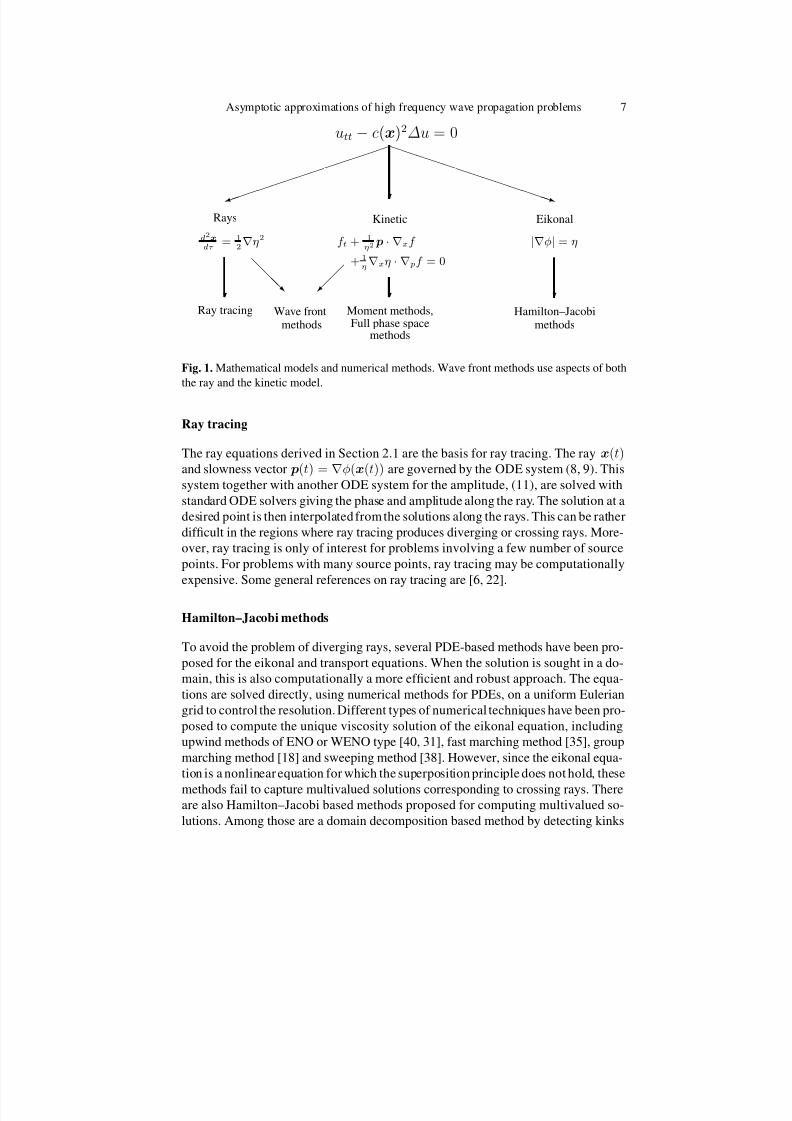
Fig. 2. A typical geometrical optics solution in two dimensions and a constant medium (c ≡ 1)

around a perfectly reflecting halfplane (a), and the same problem augmented with diffracted

waves given by GTD (b). In the geometrical optics case, region A contains two phases (inci-

dent and reflected), region B one phase (incident), and region C is in shadow, with no phases

and hence a zero solution. On the boundaries between the regions the geometrical optics so-

lution is discontinuous. Real part of a solution to the Helmholtz equation for this problem is

shown in (c). The diffracted wave is faintly visible as a circular wave centered at the halfplane

tip.

By (6) the error in standard geometrical optics solutions is of the order O(1/ω).However, the derivation of (7) from (6) does not take into account the effects of

geometry and boundary conditions. In these cases the series expansion (6) is not

adequate and extra terms must be added to match the solution to the boundary con-

ditions. These terms represent the diffracted waves. They are of the order O(1/ωα)for some α ∈ (0, 1) and hence normally much larger than the the usual error in stan-

dard geometrical optics, but still small for large frequencies. Discarding diffraction

phenomena, may therefore be too crude an approximation for a scattering problem

at moderate frequencies.

One typical improved expansion that includes diffraction terms is

u(x) = eiωφ(x)∞

k=0 Ak(x)(iω)−k +1√ω

eiωφd(x)∞

k=0 Bk(x)(iω)−k,

which is similar to the standard geometrical optics ansatz (6), only that a new

diffracted wave scaled by√

ω has been added (index d). For high frequencies, the

diffraction term B0 is also retained, together with the geometrical optics term A0.






uc

uinc

ud

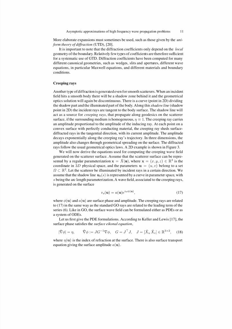
Fig. 3. Diffraction by a smooth cylinder. Top figure shows the solution schematically. The

incident field uinc induces a creeping ray uc at the north (and south) pole of the cylinder. As

the creeping ray propagates along the surface, it continuously emits surface-diffracted rays udwith exponentially decreasing initial amplitude. Bottom figure shows the real part of a solution

to the Helmholtz equation. The surface diffracted waves can be seen behind the cylinder.

One can write (18) as a Hamilton-Jacobi equation H (u, ∇φ) = 0, with the

Hamiltonian

H (u,p)≡

1

2p⊤ G−1(u)p

−η2(u)

2. (19)

Note that in the case η = constant, the rays associated with the surface eikonal

equation (18) are geodesics, or shortest paths between two points on the surface.

Henceforth, we will assume η ≡ 1.

Another formulation of the creeping wave field is based on ODEs. Introducing a

parameter τ , the bicharacteristicsu(τ ),p(τ )

are determined by the solution of the

following Hamiltonian equations

u = H p = G−1p, (20a)

p = −H u. (20b)

Here the dot denotes differentiation with respect to the parameter τ . Note thatp(τ ) =

∇φ(u(τ )) for all τ ≥ 0, as long as φ is smooth. As a consequence, from (18) and(20) we obtain that | ˙X | = |J u| = |JG−1

p| = 1, and therefore we can identify the

parameter τ with arc length along the creeping rays X (u(τ )). Setting u = ρ cos θand v = ρ sin θ, we can reduce the system (20) to






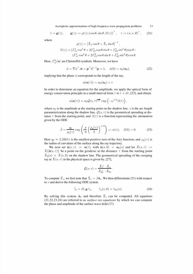
There is yet another formulation, which can be seen as an analogue to the kinetic

formulation of standard GO, [11, 28]. We introduce the phase space P = R2 × S,

where S = [0, 2 π], and consider the triplet γ = (u,v,θ) as a point in this space.

The ray trajectories on the scatterer, given by (21), are then confined to a subdomain

Ω p = Ω × S ⊂ P in phase space. We consider a ray γ (τ ) satisfying (21), starting atγ (0) = γ = (u,v,θ) ∈ Ω p and ending at the boundary ∂Ω p = ∂Ω × S. We call this

end point (U,V,Θ) ∈ ∂Ω p the escape point of the ray. See Figure 4. We then define

three types of unknown escape functions for this starting point γ , as follows:

• F : P → P, F (γ ) = (U,V,Θ) is the escape point.

• Φ : P → R is the length of the ray starting at γ and ending at F (γ ). We also refer

to this as the travel-time of the ray.

• B : P → R is the difference between the β -values at the escape and starting

points, where β satisfies (23).

(u, v)

θ

Θ(U, V )

∂Ω

Fig. 4. A ray trajectory in the parameter space, starting at γ = (u,v,θ) ∈ Ωp and ending at

the escape point F (γ ) = (U,V,Θ) ∈ ∂Ωp.

In order to derive equations for these functions, we notice that F is constant for

all γ (τ ) along the geodesic, and therefore

d

dτ F (γ (τ )) = 0 ⇒ g1 F u + g2 F v + g3 F θ = 0, γ ∈ Ω p. (25)

Here the coefficients g = (g1, g2, g3)⊤ in (25) are known and given by (21).

In the same way, by (22) and (23), we can write the equations for Φ and B. Each

escape function f (γ ) of the above types satisfies the escape PDE

g1(γ ) f u + g2(γ ) f v + g3(γ ) f θ = h(γ ), γ ∈ Ω p, (26)

where the forcing term h is 0, 1 and α(γ ) for f = F , f = Φ and f = B, respectively.The boundary condition at inflow points of ∂Ω p are

f (γ ) = b, γ ∈ ∂Ω inflow p , ∂Ω inflow

p =

γ ∈ ∂Ω p | n(γ )⊤ g(γ ) < 0

,




(a) GO (b) Helmholtz

(c) ω = 90 (d) ω = 180 (e) ω = 270

Fig. 5. Caustics generated when a plane wave is refracted by a cylinder of higher refractive

index than the surrounding media. The geometrical optics solution by ray tracing is shown in

(a), while (b) contains an actual solution of Helmholtz equation (real part). The concentration

of rays coincides with the pronounced dark/light pattern (high amplitude) in the solution.

The figures in the bottom row (c–e) show the absolute value of the Helmholtz solution in

a horizontal cut in the middle of the top figures, for increasing frequencies ω. The cylinder

boundaries are indicated by dashed lines. The amplitude away from the caustic is independent

of ω but grows slowly with ω at the caustic.

with n being the outward normal vector in the phase space. The boundary value b is

γ , 0 and 0 for f = F , f = Φ and f = B, respectively. Note that one can also derive

escape equations for computing geometrical spreading, using the ODE (24).The escape equation (26) is a linear hyperbolic equation, and the variable velocity

coefficients g = (g1, g2, g3)⊤ are known and determine the characteristic direction

at every point γ ∈ Ω p. One important property of the solutions to the escape PDEs

is that they are in general discontinuous due to discontinuous boundary conditions.

Caustics

Close to caustics the amplitude grows rapidly in the geometrical optics approxima-

tion and blows up at the caustic itself. In reality the amplitude remains bounded, but

increases with the frequency ω, see Figure 5. The error in the standard series expan-

sion (6) is thus unbounded around caustics. To capture the actual solution behavior

there are better expansions that have small errors uniformly in ω, derived e.g. byLudwig [25] and Kravtsov [21]. The expansions are different for different types of

caustics. For a fold caustic there are two ray families meeting at the caustic, with

phases φ+ and φ−. Letting ρ = 34(φ+ − φ−) a more suitable description of the




solution u in this case is

u(x) = ω1/6 eiωφ(x)

Ai(−(ωρ(x))2/3)

∞

k=0Ak(x)(iω)−k

+ iω−1/3Ai′(−(ωρ(x))2/3)∞

k=0

Bk(x)(iω)−k

,

where Ai is the Airy function. The dominant term close to the caustic, |ρ|ω ≪ 1 is of

the order O(ω1/6) with an error of O(ω−1/3). Away from the caustic, on the convex

side where ρ > 0, we can use the fact that |Ai(−x)| ∼ x−1/4 and |Ai′(−x)| ∼ x1/4

for large x, to conclude that the dominant term is of the order O(1) with an error of

O(ω−1), i.e. the standard situation for geometrical optics.

3.2 Numerical methods

The diffracted rays generated by discontinuities and shed by creeping rays obey theusual geometrical optics equations. The main computational task is thus based on

the standard GO approximation discussed in Section 2. However, computing creep-

ing ray contribution to the field involves more technicalities, and one needs to find

geodesics on the scatterer surface as well. We therefore here discuss computation of

creeping rays in more detail. We then review numerical methods for computing the

wave field at caustics.

Creeping rays computation

There are different numerical techniques for computing creeping rays. Similar to the

numerical methods in standard GO, these techniques have advantages and disadvan-

tages. Here, we will briefly review the methods based on the surface ray equations

and surface eikonal/transport equations. We then discuss in more detail a new method

based on the escape equations.

Lagrangian techniquesare based on surface ray equations. The simplest and most

common method is standard ray tracing which solves these ODEs on triangulated

surfaces [14]. Assuming the geodesic paths are given by piecewise linear curves,

it is possible to find the linear ray path on each triangle, analytically. This method

gives the surface phase and amplitude solutions along creeping rays. Interpolation

must then be applied to obtain the solution everywhere. But, in regions where rays

cross or diverge this can be rather difficult. However, the interpolation can be sim-

plified by using wave front methods [41, 12] in which, instead of individual rays,

an interface representing a wave front is evolved. Nevertheless, for some problems,

such as RCS where creeping rays from all illumination angles must be computed,

Lagrangian methods can be computationally expensive.Eulerian techniques are based on surface eikonal and surface transport equations.

These PDEs are discretized on fixed computational grids, and there is no problem

with interpolation [19]. However, these equations only give the correct solution when




it is a single wave. In the case of crossing waves, more elaborate schemes have been

devised to capture multivalued solutions, [27, 42].

We now discuss an adaptation of the fast phase space method, [11], for standard

geometrical optics to computation of creeping waves, presented in [27]. This method

is based on the escape equations (26). As a first step, the escape equations mustbe solved numerically. There are different approaches for solving (26). One is to

discretize the PDEs in the phase space using a finite difference or finite volume

approximation and arrive at a system of linear equations Af = b, where A is a sparse

N 3×N 3 matrix, with N being the number of grid points in each coordinate direction

of Ω p, and b represents the boundary conditions. This system can then be solved

iteratively, and one can speed up the computations using suitable preconditioners [5].

However, in the case that characteristics change direction many times in the phase

space domain, it is difficult to find good preconditioners. Another way to solve the

escape equations is to write them as

f t + g1 f u + g2 f v + g3 f θ = h,

and solve these time-dependent equations until the steady state f t = 0. However,finding a fast algorithm which is not much restricted by the CFL condition is anal-

ogous to finding a good preconditioner in the iterative method. Yet, another method

is a version of fast marching algorithm given by Fomel and Sethian [11]. The basic

idea of the algorithm is to march the solution outwards from the boundary and use

the characteristic directions to update grid values by interpolating them from their

known neighboring grid points. Note that since the solutions to the escape PDEs

can be discontinuous, it is important to use suitable interpolation techniques, such

as essentially non-oscillatory (ENO) interpolations, to avoid the unphysical Gibbs

oscillations. The algorithm is of complexity O(N 3 log N ).

The escape PDEs solutions contain information about all possible creeping rays

in all directions. To extract properties like phase and amplitude for a ray family, post-

processing of the solution is needed. We first note that F (u1, v1, θ1) = F (u2, v2, θ2)implies that (u1, v1, θ1) and (u2, v2, θ2) lie on the same geodesic. Suppose we want

to compute the surface phase at a point on the illuminated scatterer. We assume that

the shadow line γ 0(s) in known. For each point u ∈ Ω covered by the surface wave,

there is at least one creeping ray, starting at the shadow line, which passes through

it. We can thus find s = s∗(u) and phase angle θ = θ∗(u), as the solution to

F (γ 0(s)) = F (u, θ). (27)

The phase at u is then given by

φ(u) = φ0(u0(s∗)) + Φ(γ 0(s∗)) − Φ(γ ∗), γ ∗ = (u, θ∗) ∈ L(γ 0),

whereL(γ 0) is a sub-manifold of phase space P on which the creeping rays generated

at γ 0(s) lie. Note that there may be multiple solutions (s∗, θ∗) to (27), giving multiplephases. Using the same technique, the amplitude can also be computed.

To solve (27), we note that since F is a point on the phase space boundary, it can

be reduced to a point in R2. The left and right hand sides of (27) are then curves in




R2, and solving (27) amounts to finding crossing points of these curves. Discretizing

the shadow line in N grid points, we need to find crossing points of two complex

lines of N straight line segments, which can be done in O(N ). For all N 2 points

on the scatterer surface, the computational cost for solving (27) will be

O(N 3). The

total complexity, including solving the escape PDEs and solving (27), is thereforeO(N 3 log N ). This is expensive for computing the field for only one shadow line.

For example by using wave front tracking or solvers based on the surface eikonal

equation, the complexity is O(N 2). However, if the solutions are sought for many

shadow lines and only a few points on the scatterer, the phase space method is more

efficient. One such example is computing the monostatic radar cross sections (RCS).

The method described above requires one fixed parameterization X (u) of the

scatterer. It has however been modified in [28] for more complex scatterer surfaces

which cannot be represented by a single non-singular explicit parameterization. The

surface is split into several simpler surfaces with explicit parameterizations. These

multiple patches collectively cover the scatterer surface in a non-singular manner.

The escape PDEs are solved in every patch, individually. The creeping rays on the

scatterer are then computed by connecting all individual solutions through a fastpost-processing. The inter-patch boundaries are treated by the continuity of creeping

rays.

Wave field computation at caustics

Here we focus on the Gaussian beam method for computing the wave field at caus-

tics. See [4] for another method based on the GO approximation.

The Gaussian beam method is an asymptotic method for computing high-frequency

wave fields in smoothly varying inhomogeneous media. It was proposed by Popov

[32], based on an earlier work of Babic and Pankratova [1]. Gaussian beams are

closely related to ray tracing, but instead of viewing rays just as characteristics of

the eikonal equation, Gaussian beams are fatter rays: They are approximate highfrequency solution to the wave equation or the Helmholtz equation which are con-

centrated on a standard ray. Contrary to standard GO rays, Gaussian beams accept

complex valued phase functions. The main advantage of this construction is that

Gaussian beams give the correct solution also at caustics where standard geometrical

optics breaks down.

We now review the governing equations. We consider a ray in a two-dimensional

Cartesian coordinate system x, y given by the ray tracing system (12). In orthogonal

ray-centered coordinates (t, q), where q is the axis perpendicular to the ray at point twith the origin on the ray, the paraxial Gaussian beam solution closely concentrated

about the central ray is given by

u(t,q,ω) = A(t, q) exp

iωφ(t, q)

, (28)

where the complex-valued amplitude A and the phase φ are given by the eikonal and

transport equations with complex initial data for φ. They are approximated by Taylor

expansions






7. M. G. Crandall and P.-L. Lions. Viscosity solutions of Hamilton-Jacobi equations. Trans.

Amer. Math. Soc., 277(1):1–42, 1983.

8. B. Engquist and O. Runborg. Computational high frequency wave propagation. Acta

Numerica, 12:181–266, 2003.

9. B. Engquist, O. Runborg, and A.-K. Tornberg. High frequency wave propagation by thesegment projection method. J. Comput. Phys., 178:373–390, 2002.

10. E. Fatemi, B. Engquist, and S. J. Osher. Numerical solution of the high frequency asymp-

totic expansion for the scalar wave equation. J. Comput. Phys., 120(1):145–155, 1995.

11. S. Fomel and J. A. Sethian. Fast phase space computation of multiple arrivals. Proc. Natl.

Acad. Sci. USA, 99(11):7329–7334 (electronic), 2002.

12. S. Hagdahl. Hybrid Methods for Computational Electromagnetics in Frequency Domain.

PhD thesis, NADA, KTH, Stockholm, 2005.

13. L. Hormander. The analysis of linear partial differential operators. I-IV . Springer-Verlag,

Berlin, 1983–1985.

14. P. E. Hussar, V. Oliker, H. L. Riggins, E.M. Smith-Rowlan, W.R. Klocko, and L. Prussner.

An implementation of the UTD on facetized CAD platform models. IEEE Antennas

Propag., 42(2):100–106, 2000.

15. S. Jin and X. Li. Multi-phase computations of the semiclassical limit of the Schrodinger

equation and related problems: Whitham vs. Wigner. Physica D, 182(1-2):46–85, 2003.

16. J. Keller. Geometrical theory of diffraction. J. Opt. Soc. Amer., 52, 1962.

17. J. Keller and R. M. Lewis. Asymptotic methods for partial differential equations: the

reduced wave equation and Maxwell’s equations. Surveys Appl. Math., 1:1–82, 1995.

18. S. Kim. An O(N ) level set method for eikonal equations. SIAM J. Sci. Comput.,

22(6):2178–2193, 2000.

19. R. Kimmel and J. A. Sethian. Computing geodesic paths on manifolds. Proc. Natl. Acad.

Sci. USA, 95(15):8431–8435 (electronic), 1998.

20. R. G. Kouyoumjian and P. H. Pathak. A uniform theory of diffraction for an edge in a

perfectly conducting surface. Proc. IEEE , 62(11):1448–1461, 1974.

21. Yu. A. Kravtsov. On a modification of the geometrical optics method. Izv. VUZ Radiofiz.,

7(4):664–673, 1964.

22. R. T. Langan, I. Lerche, and R. T. Cutler. Tracing of rays through heterogeneous media:

An accurate and efficient procedure. Geophysics, 50:1456–1465, 1985.23. B. R. Levy and J. Keller. Diffraction by a smooth object. Comm. Pure Appl. Math., 12,

1959.

24. H. Liu, S. Osher, and R. Tsai. Multi-valued solution and level set methods in computa-

tional high frequency wave propagation. Commun. Comput. Phys., 1(5):765–804, 2006.

25. D. Ludwig. Uniform asymptotic expansions at a caustic. Comm. Pure Appl. Math.,

19:215–250, 1966.

26. V. P. Maslov. Th´ eorie des perturbations et m´ ethodes asymptotiques. Izd. Moskov. Univ.,

1965. (In Russian). French translation, Dunod, Paris, 1972.

27. M. Motamed and O. Runborg. A fast phase space method for computing creeping rays.

J. Comput. Phys., 219(1):276–295, 2006.

28. M. Motamed and O. Runborg. A multiple-patch phase space method for computing tra-

jectories on manifolds with applications to wave propagation problems. Commun. Math.

Sci., 5(3):617–648, 2007.

29. M. Motamed and O. Runborg. A wave front Gaussian beam method for high-frequencywave propagation. In WAVES 2007 , University of Reading, UK, 2007.

30. S. J. Osher and J. A. Sethian. Fronts propagating with curvature-dependent speed: algo-

rithms based on Hamilton-Jacobi formulations. J. Comput. Phys., 79(1):12–49, 1988.



Documents

Asymptotic approximations of high frequency wave propagation problems