ASYMPTOTIC ANALYSIS OF STRUCTURED DETERMINANTS VIA THE

RIEMANN-HILBERT APPROACH

A Dissertation

Submitted to the Faculty

of

Purdue University

by

Roozbeh Gharakhloo

In Partial Fulfillment of the

Requirements for the Degree

of

Doctor of Philosophy

August 2019

Purdue University

Indianapolis, Indiana

ii

THE PURDUE UNIVERSITY GRADUATE SCHOOL

STATEMENT OF DISSERTATION APPROVAL

Dr. Pavel Bleher

Department of Mathematical Sciences

Dr. Alexandre Eremenko

Department of Mathematics, Purdue University

Dr. Alexander Its, Chair

Department of Mathematical Sciences

Dr. Maxim Yattselev

Department of Mathematical Sciences

Approved by:

Dr. Evgeny Mukhin

Director of the Graduate Programs, Department of Mathematical Sciences

iii

iv

v

ACKNOWLEDGMENTS

First and foremost, I would like to express my deepest gratitude to professor Alexander

Its. I have been very fortunate to be the student of a mathematician of his caliber. Someone

who is unquestionably one of the distinguished authorities in the modern theory of integrable

systems and specifically the Riemann-Hilbert method. I would like to thank him for all the

invaluable lessons that he has most humbly taught me through our mathematical and personal

exchanges. I will always be indebted to him for his impact on my education and I hope that

I may continue to learn from him and his works in the years to come.

I would also like to thank my Ph.D. committee members. Professor Pavel Bleher and

professor Maxim Yattselev have both had a great impact on my understanding of mathematics.

Here I express my sincere gratitude for all that I have learned from them. I would like to also

thank professor Alexandre Eremenko for reading the thesis and for fulfilling his role on my

Ph.D. defense committee.

I highly appreciate the impact of my non-IUPUI collaborators on this thesis. I am grateful

to Dr. Christophe Charlier, who gave me the opportunity and encouragement to collaborate

with him on a continuation of his earlier work. This collaboration and our discussions have

been significantly instructive and I deeply appreciate that. I am also thankful to professor

Karol Kozlowski for our collaboration which broadened the scope of my research and moti-

vated me to learn more about his research objectives. I am also very thankful to professors

Estelle Basor, Torsten Ehrhardt, Jani Virtanen, and Nicholas Witte with whom I have had

the privilege to discuss mathematical issues related to this thesis. I am looking forward to

hopefully see those discussions in the form of concrete research projects in a near future.

The time that I have been a part of the department of mathematical sciences at IUPUI

is filled with fantastic moments of educational and personal growth. I would like to thank

professors Carl Cowen, William Geller, Ronghui Ji, Slawomir Klimek, Evgeny Mukhin, Daniel

Ramras, Roland Roeder, Joseph Rosenblatt, and Vitaly Tarasov for working with me in

vi

various contexts for my mathematical development. I am very thankful to professor Bruce

Kitchens for the help and encouragement he gave me to apply to IUPUI when I was in Iran.

I would also like to thank the department chair, professor Jeffrey Watt and the respected

staff Jamie Beer, Tina Carmichael, Alex Duncan, John Fullam, Jamie Linville, Kelly Houser

Matthews, Cindy Ritchie, and Zachary Smith for all the help that they have sincerely offered.

I will never forget the help of my dear firend Hassan Behrouzvaziri in various occasions at

the beginning of my studies at IUPUI and thus my special thanks goes to him for his kind

support. I would also like to thank my fellow graduate students, especially those who tried

to create an atmosphere of friendship, support, collaboration, and motivation.

The professors at Shiraz University, where I did my B.Sc. in mechanical engineering, have

had a significant impact on my life and I am highly indebted to them as they set up the

path for me to complete the Ph.D. program here at IUPUI. My most special thanks goes to

professor Mojtaba Mahzoon. Apart from his remarkable and unforgettable impact on me at

a personal level, he was the one who opened up my eyes to the beautiful and rich world of

mathematics when I attended his lectures on dynamical systems and advanced mathematics.

He was the one who encouraged me to be brave enough to make a shift in my studies from

mechanical engineering to pure mathematics. I am almost sure that I would not be writing this

thesis now if I have not met him in my life. I would also like to thank professor Mohammad

Rahim Hematyian for his help regarding this transition as the dean of School of Mechanical

Engineering at Shiraz University. I am also grateful to professors Homayoun Emdad and

Mohammad Eghtesad for all that I have learned from them back in Shiraz University. I

sincerely express my gratitude for all the advice and encouragement that I received from

professor Bahman Gharesifard. Many thanks to Dr.Hamed Farokhi and Dr.Saber Jafarpour

for all of their motivations early on which made me think more seriously about applying to

universities abroad. I also highly appreciate Alisina Azhang for being a great motivator and

companion in our transition from mechanical engineering to pure mathematics.

The principal of the high school I went to, Mr. Ghasem Ne’mati, is and will remain to be

a truly special person in my life. As he might read this acknowledgment at some point and

might have forgotten a former student whom he has not met in at least fourteen years, I would

vii

like to briefly mention the story of his contribution to my education, hoping that he might

recall the person who is thanking him in this paragraph. In the first year of high school I was

not doing very well in mathematics for several reasons which shall not be discussed here. My

score in mathematics was not good enough to continue as a math major and I was planning

to choose a different path for my second year in high school. Mr. Ne’mati reached out to my

parents and raised the question that how is it possible that I am not doing fine in math while

being good at chess (In my age group I was among the top players in the state and later won

a gold medal in national high school championship). To him, It made no sense that I could

not score well in mathematics. He was obviously uncomfortable about my poor performance,

perhaps more than myself or my parents, and insisted strongly that I should retake the math

exam in the summer, and in case I get a high enough score, I should continue in mathematics.

Thanks to his genuine care for a student who was doing poorly in mathematics, I not only

continued as a math major in the rest of my high school years, but more surprisingly, here I

am finishing a PhD program in pure mathematics. Those few minutes that he took to reflect

upon the imbalance between a student’s abilities and his performance, entirely changed the

way my life unfolded for the better (I think), and I would like to express my most sincere

gratitude to him, not only for his impact on my life but most importantly for teaching me the

importance of a single genuine care for others.

I should assert that words can not do justice to admire the exceptional role of my wife,

Asma, in this accomplishment. She has always been by my side in all the twists and turns and

this thesis may not have been concluded without her exemplary support and love. Finally, I

would like to express my deepest gratitude to my dear family in Iran, specifically my mother,

for all the love and care that I have continuously received from them throughout the years.

viii

TABLE OF CONTENTS

Page

LIST OF FIGURES . . . . . . . . . . . . . . . . . . . . . . . . . . . . . . . . . . . . . . xi

ABBREVIATIONS . . . . . . . . . . . . . . . . . . . . . . . . . . . . . . . . . . . . . . . xii

ABSTRACT . . . . . . . . . . . . . . . . . . . . . . . . . . . . . . . . . . . . . . . . . xiii

1 INTRODUCTION . . . . . . . . . . . . . . . . . . . . . . . . . . . . . . . . . . . . . 11.1 Definitions, notations and preliminaries . . . . . . . . . . . . . . . . . . . . . . . 11.2 Selected Riemann-Hilbert problems . . . . . . . . . . . . . . . . . . . . . . . . . 4

1.2.1 The RHP for Toeplitz determinants . . . . . . . . . . . . . . . . . . . . . 41.2.2 The RHP for Hankel determinants . . . . . . . . . . . . . . . . . . . . . 61.2.3 The RHP for integrable integral operators . . . . . . . . . . . . . . . . . 11

2 ASYMPTOTICS OF HANKEL DETERMINANTS WITH A LAGUERRE-TYPEOR JACOBI-TYPE POTENTIAL AND FISHER-HARTWIG SINGULARITIES . . . 142.1 Introduction . . . . . . . . . . . . . . . . . . . . . . . . . . . . . . . . . . . . . . 142.2 A Riemann-Hilbert problem for orthogonal polynomials . . . . . . . . . . . . . . 302.3 Differential identities . . . . . . . . . . . . . . . . . . . . . . . . . . . . . . . . . 32

2.3.1 Identity for ∂ν logLn(~α, ~β, 2(x+ 1), 0) with ν ∈ α0, . . . , αm, β1, . . . , βm . 322.3.2 A general differential identity . . . . . . . . . . . . . . . . . . . . . . . . 35

2.4 Steepest descent analysis . . . . . . . . . . . . . . . . . . . . . . . . . . . . . . . 362.4.1 Equilibrium measure and g-function . . . . . . . . . . . . . . . . . . . . . 362.4.2 First transformation: Y 7→ T . . . . . . . . . . . . . . . . . . . . . . . . 382.4.3 Second transformation: T 7→ S . . . . . . . . . . . . . . . . . . . . . . . 392.4.4 Global parametrix . . . . . . . . . . . . . . . . . . . . . . . . . . . . . . 422.4.5 Local parametrix near tk, 1 ≤ k ≤ m . . . . . . . . . . . . . . . . . . . . 452.4.6 Local parametrix near 1 . . . . . . . . . . . . . . . . . . . . . . . . . . . 462.4.7 Local parametrix near −1 . . . . . . . . . . . . . . . . . . . . . . . . . . 482.4.8 Small norm RH problem . . . . . . . . . . . . . . . . . . . . . . . . . . . 49

2.5 Starting points of integration . . . . . . . . . . . . . . . . . . . . . . . . . . . . 542.6 Integration in ~α and ~β for the Laguerre weight . . . . . . . . . . . . . . . . . . . 56

2.6.1 Asymptotics for ∂ν logLn(~α, ~β, 2(x+ 1), 0), ν ∈ α0, . . . , αm, β1, . . . , βm . 592.6.2 Integration in α0 . . . . . . . . . . . . . . . . . . . . . . . . . . . . . . . 632.6.3 Integration in α1, . . . , αm . . . . . . . . . . . . . . . . . . . . . . . . . . . 632.6.4 Integration in β1, . . . , βm . . . . . . . . . . . . . . . . . . . . . . . . . . . 65

2.7 Integration in V . . . . . . . . . . . . . . . . . . . . . . . . . . . . . . . . . . . . 672.7.1 Deformation parameters s . . . . . . . . . . . . . . . . . . . . . . . . . . 672.7.2 Some identities . . . . . . . . . . . . . . . . . . . . . . . . . . . . . . . . 68

ix

Page

2.7.3 Integration in s for Laguerre-type weights . . . . . . . . . . . . . . . . . 702.7.4 Jacobi-type weights . . . . . . . . . . . . . . . . . . . . . . . . . . . . . . 74

2.8 Integration in W . . . . . . . . . . . . . . . . . . . . . . . . . . . . . . . . . . . 76

3 A RIEMANN-HILBERT APPROACH TO ASYMPTOTIC ANALYSIS OF TOEPLITZ+ HANKEL DETERMINANTS . . . . . . . . . . . . . . . . . . . . . . . . . . . . . . 783.1 Introduction and preliminaries . . . . . . . . . . . . . . . . . . . . . . . . . . . . 783.2 Toeplitz + Hankel determinants: Hankel weight supported on T . . . . . . . . . 813.3 The steepest descent analysis for r = s = 1. . . . . . . . . . . . . . . . . . . . . 85

3.3.1 The associated 2× 4 and 4× 4 Riemann-Hilbert problems . . . . . . . . 853.3.2 Relation of the 2× 4 and 4× 4 Riemann-Hilbert problems . . . . . . . . 873.3.3 Undressing of the X -RHP . . . . . . . . . . . . . . . . . . . . . . . . . . 883.3.4 Normalization of behaviours at 0 and ∞ . . . . . . . . . . . . . . . . . . 903.3.5 Opening of the lenses . . . . . . . . . . . . . . . . . . . . . . . . . . . . . 933.3.6 The global parametrix and a model Riemann-Hilbert problem . . . . . . 943.3.7 A solvable case . . . . . . . . . . . . . . . . . . . . . . . . . . . . . . . . 953.3.8 The small-norm Riemann-Hilbert problem associated to Dn(φ, dφ, 1, 1) . 983.3.9 Asymptotics of hn . . . . . . . . . . . . . . . . . . . . . . . . . . . . . 101

3.4 Suggestions for future work . . . . . . . . . . . . . . . . . . . . . . . . . . . . 1063.4.1 Ising model on different half-planes/Extension of the results to general

offset values r, s 6= 1. . . . . . . . . . . . . . . . . . . . . . . . . . . . . 1063.4.2 Extension to Fisher-Hartwig symbols . . . . . . . . . . . . . . . . . . . 1093.4.3 Characteristic polynomial of a Hankel matrix . . . . . . . . . . . . . . 110

4 ASYMPTOTIC ANALYSIS OF A BORDERED-TOEPLITZ DETERMINANT ANDTHE NEXT-TO-DIAGONAL CORRELATIONS OF THE ANISOTROPIC SQUARELATTICE ISING MODEL . . . . . . . . . . . . . . . . . . . . . . . . . . . . . . . . 1124.1 Introduction and Background . . . . . . . . . . . . . . . . . . . . . . . . . . . 1124.2 determinantal formula for next-to-diagonal correlations . . . . . . . . . . . . . 115

5 EMPTINESS FORMATION PROBABILITY IN THE XXZ-SPIN 1/2 HEISEN-BERG CHAIN . . . . . . . . . . . . . . . . . . . . . . . . . . . . . . . . . . . . . . 1215.1 Introduction . . . . . . . . . . . . . . . . . . . . . . . . . . . . . . . . . . . . . 121

5.1.1 The Y - RH problem . . . . . . . . . . . . . . . . . . . . . . . . . . . . 1245.2 The differential identity for the Fredholm determinant . . . . . . . . . . . . . . 1255.3 The Riemann-Hilbert analysis . . . . . . . . . . . . . . . . . . . . . . . . . . . 128

5.3.1 Mapping onto a fixed interval . . . . . . . . . . . . . . . . . . . . . . . 1285.3.2 g - function transformation . . . . . . . . . . . . . . . . . . . . . . . . . 1295.3.3 Global parametrix . . . . . . . . . . . . . . . . . . . . . . . . . . . . . 1315.3.4 The local parametrix at z = 1 . . . . . . . . . . . . . . . . . . . . . . . 132

5.4 Asymptotics of the determinant . . . . . . . . . . . . . . . . . . . . . . . . . . 137

REFERENCES . . . . . . . . . . . . . . . . . . . . . . . . . . . . . . . . . . . . . . . . 140

A NORMALIZED SMALL-NORM RIEMANN-HILBERT PROBLEMS . . . . . . . . 144

x

Page

B SOLUTION OF THE RIEMANN-HILBERT PROBLEM ASSOCIATED WITH THEANISOTROPIC SQUARE LATTICE ISING MODEL IN THE LOW TEMPERA-TURE REGIME . . . . . . . . . . . . . . . . . . . . . . . . . . . . . . . . . . . . . 147

C AIRY, BESSEL AND CONFLUENT HYPERGEOMETRIC MODEL RIEMANN-HILBERT PROBLEMS . . . . . . . . . . . . . . . . . . . . . . . . . . . . . . . . . 152C.1 Airy model RH problem . . . . . . . . . . . . . . . . . . . . . . . . . . . . . . 152C.2 Bessel model RH problem . . . . . . . . . . . . . . . . . . . . . . . . . . . . . 153C.3 Confluent hypergeometric model RH problem . . . . . . . . . . . . . . . . . . 155

VITA . . . . . . . . . . . . . . . . . . . . . . . . . . . . . . . . . . . . . . . . . . . . . 159

xi

LIST OF FIGURES

Figure Page

1.1 The jump contour for the Riemann-Hilbert problem (Σ,J ). . . . . . . . . . . . . . 2

2.1 The jump contour for the RH problem for S with m = 2 and a Laguerre-typeweight. For Jacobi-type weights, the jump contour for S is of the same shape,except that there are no jumps on (1,+∞). . . . . . . . . . . . . . . . . . . . . . . 40

2.2 The neighborhood Dtk and its image under the mapping ftk . . . . . . . . . . . . . . 45

2.3 Jump contour ΣR for the RH problem for R for Laguerre-type weights with m = 2.For Jacobi-type weights, ΣR is of the same shape except that there are no jumpson (1,∞) \ D1. . . . . . . . . . . . . . . . . . . . . . . . . . . . . . . . . . . . . . . 51

3.1 The jump contour for the Z-RHP . . . . . . . . . . . . . . . . . . . . . . . . . . . . 89

3.2 The jump contour for the S-RHP . . . . . . . . . . . . . . . . . . . . . . . . . . . . 94

5.1 The contour Γα . . . . . . . . . . . . . . . . . . . . . . . . . . . . . . . . . . . . . 122

B.1 Opening of lenses: the jump contour for the S-RHP. . . . . . . . . . . . . . . . . 148

C.1 The jump contour ΣAi for ΦAi. . . . . . . . . . . . . . . . . . . . . . . . . . . . . . 153

C.2 The jump contour ΣBe for ΦBe(ζ). . . . . . . . . . . . . . . . . . . . . . . . . . . . 155

C.3 The contour ΣHG = ∪8k=1Γk. Each Γk extends to ∞ and forms an angle π

4with its

adjacent ray. . . . . . . . . . . . . . . . . . . . . . . . . . . . . . . . . . . . . . . . 156

xii

ABBREVIATIONS

RHP Riemann-Hilbert problem

LUE Laguerre Unitary Ensemble

GUE Gaussian Unitary Ensemble

JUE Jacobi Unitary Ensemble

FH Fisher-Hartwig

OP Orthogonal Polynomial

CLT Central Limit Theorem

xiii

ABSTRACT

Gharakhloo, Roozbeh. Ph.D., Purdue University, August 2019. Asymptotic Analysis of Struc-tured Determinants via the Riemann-Hilbert Approach. Major Professor: Alexander Its.

In this work we use and develop Riemann-Hilbert techniques to study the asymptotic

behavior of structured determinants. In chapter one we will review the main underlying

definitions and ideas which will be extensively used throughout the thesis. Chapter two is

devoted to the asymptotic analysis of Hankel determinants with Laguerre-type and Jacobi-

type potentials with Fisher-Hartwig singularities. In chapter three we will propose a Riemann-

Hilbert problem for Toeplitz+Hankel determinants. We will then analyze this Riemann-

Hilbert problem for a certain family of Toeplitz and Hankel symbols. In Chapter four we

will study the asymptotics of a certain bordered-Toeplitz determinant which is related to

the next-to-diagonal correlations of the anisotropic Ising model. The analysis is based upon

relating the bordered-Toeplitz determinant to the solution of the Riemann-Hilbert problem

associated to pure Toeplitz determinants. Finally in chapter five we will study the emptiness

formation probability in the XXZ-spin 1/2 Heisenberg chain, or equivalently, the asymptotic

analysis of the associated Fredholm determinant.

1

1. INTRODUCTION

1.1 Definitions, notations and preliminaries

The work in this thesis is focused on the asymptotic analysis of structured determinants

arising in random matrix theory, statistical mechanics, theory of integrable operators and

theory of orthogonal polynomials, where we primarily employ the Riemann-Hilbert method.

For a given oriented contour Σ in the complex plane (see Figure 1.1) and a function J :

Σ→ GL(k,C), the (normalized) Riemann-Hilbert problem (Σ,J ) consists of determining the

unique k × k matrix function Y (z) satisfying

• Y (z) is analytic in C \ Σ,

• Y+(z) = Y−(z)J (z), for z ∈ Σ, and

• Y (z)→ I, as z →∞,

where J (z) is called the jump matrix of the Riemann-Hilbert problem (RHP), and Y±(z)

denote the limit of Y (ζ) as ζ approaches z ∈ Σ from the ± side of the oriented contour Σ: As

we move along a path in Σ in the direction of the orientation, by convention we say that the

+ side (respectively the - side) lies to the left (respectively right).

By structured determinants, we mean Toeplitz, bordered Toeplitz, Hankel, Toeplitz+Hankel

and integrable Fredholm determinants which arise almost ubiquitously in random matrix the-

ory and statistical mechanics. The n×n Toeplitz and Hankel matrices associated respectively

to the symbols φ and w are respectively defined as

Tn[φ] := φj−k, j, k = 0, · · · , n− 1, φk =

∫Tz−kφ(z)

dz

2πiz, (1.1.1)

and

Hn[w] := wj+k, j, k = 0, · · · , n− 1, wk =

∫Ixkw(x)dx, (1.1.2)

2

where I ⊂ R and T denotes the positively oriented unit circle. In the above definition, j is the

index of rows and k is the index of columns. The n× n Toeplitz + Hankel matrix associated

to these symbols is naturally defined as Tn[φ] + Hn[w]. A bordered-Toeplitz matrix has the

structure of a regular Toeplitz matrix except for its last row or column, i.e. it is of the typeφ0 φ−1 · · · φ−n+2 b−n+1

φ1 φ0 · · · φ−n+3 b−n+2

.... . . . . .

......

φn−1 φn−2 · · · φ1 b0

.

The Hankel and Toeplitz+Hankel determinants are of interest both when the Hankel

symbol w is supported on an interval and also when it is supported on the unit circle; in the

former, wk is the k-th moment of the weight as defined in (1.1.2) and in the latter wk is the

Fourier coefficient of the weight w:

wk =

∫Tz−kw(z)

dz

2πiz. (1.1.3)

For a Toeplitz or Hankel determinant with symbols supported on the unit circle, the so-

called index or winding number of a symbol φ is defined as follows: for z ∈ T write φ(z) =

|φ(z)| exp [2πib(z)] for some choice of b, then the increment of b as the result of a counter-

clockwise circuit around T is an integer solely dependent on φ (not on the choice of b), this

integer is normally referred to as the winding number or the index of the symbol φ and plays

an important role in the analysis of the generated determinants.

Σ :

+–

–+

–++ –

+–

+–

+–

Figure 1.1. The jump contour for the Riemann-Hilbert problem (Σ,J ).

3

An important class of Toeplitz or Hankel symbols are those with the so-called Fisher-Hartwig

singularities. These singularities are named after Fisher and Hartwig, due to their pioneering

work in their identification [1]. We say that a symbol φ defined on the unit circle possesses

Fisher-Hartwig (FH) singularities if it is of the type:

φ(z) = eW (z)z∑mj=0 βj

m∏j=0

|z − zj|2αjgj(z)z−βjj , z = eiθ, θ ∈ [0, 2π), (1.1.4)

for some m = 0, 1, · · · , where zj = eiθj , j = 0, · · · ,m, θj ∈ [0, 2π),

gj(z) =

eiπβj , 0 ≤ arg z < θj,

e−iπβj , θj ≤ arg z < 2π,

(1.1.5)

where in (1.1.4) and (1.1.5) one assumes that

<αj > −1

2, βj ∈ C, j = 0, · · · ,m. (1.1.6)

The term eW (z) in (1.1.4) is sometimes referred to as the smooth part, or the Szego part of

the symbol, while the rest of the terms in (1.1.4) is sometimes referred to as the pure Fisher-

Hartwig part (e.g. see [2]). Usually, the singularities |z − zj|2αj and gj are respectively called

the ”root-type” and ”jump-type” singularities. One can also consider Hankel weights with

FH singularities on the real line(e.g. see [3–5] for particular cases); In chapter 2 we will define

such weights as part of a more general class of weights, i.e. weights with Szego part, FH part

and exponentially varying part e−nV (z), for a potential V .

Let Σ be an oriented contour in C, an integral operator acting on L2(Σ) = L2(Σ, |dz|) is

integrable if it has a kernel of the form

K(z, λ) =

∑Nj=1 fj(z)hj(λ)

z − λ, z, λ ∈ Σ, (1.1.7)

for some functions fi, hj, 1 ≤ i, j ≤ N < ∞. An integrable Fredholm determinant is of the

form det(1−K), where 1 is the identity operator and the determinant is taken in L2(Σ).

For certain choices of symbols, and integrable Fredholm operators, the corresponding struc-

tured determinants identify important objects in statistical mechanics and random matrix

4

theory. On these occasions, an asymptotic question in random matrix theory or statistical

mechanics can be translated into the question of large-n asymptotics of the corresponding

structured determinant. There is an inherent correspondence between these structured deter-

minants and a set of orthogonal polynomials associated to the symbol or integrable operator

under consideration. The groundbreaking discovery of Fokas, Its and Kitaev [6], provided

the representation of the solution to a certain 2 × 2 Riemann-Hilbert problem in terms of

the corresponding orthogonal polynomials and their Cauchy transforms; thus if the Riemann-

Hilbert problem could be solved, by independent means, for large values of the parameter

n, consequently the large-n asymptotics of associated orthogonal polynomials and structured

determinants could be found as well. The celebrated non-linear steepest descent method of

Dieft and Zhou [7] was the next paramount breakthrough which provided the needed appa-

ratus for asymptotically solving the Riemann-Hilbert problems with oscillatory jumps in n.

In this method one tries to solve an equivalent Riemann-Hilbert problem on an augmented

contour, such that the jump matrices on the new set of contours (the so-called lenses) con-

verge to the identity matrix away from intersection points of lenses and the old contour for

large values of the parameter n, and the jump matrices on the the other parts of the contour

are such that they can be factorized to produce the so-called global parametrix (away from

intersection points of lenses with the old contour) and local parametrices (in a neighborhood

of intersection points of lenses with the old contour).

1.2 Selected Riemann-Hilbert problems

In this section, we will review the Riemann-Hilbert problems associated to the structured

determinants studied in this work.

1.2.1 The RHP for Toeplitz determinants

Given a sufficiently smooth symbol φ ∈ L1(T), one can consider the associated sets of

bi-orthonormal polynomials Qn(z)∞n=0 and Qn(z)∞n=0, where Qn(z) = κnzn + lnz

n−1 + · · · ,

and Qn(z) = κnzn + lnz

n−1 + · · · satisfy the bi-orthonormality conditions

5

∫TQn(z)Qn(z−1)φ(z)

dz

2πiz= δnk. (1.2.1)

The key fact which relates these polynomials to the Toeplitz determinant with symbol φ, is

that they have determinantal representations given by

Qn(z) =1√

detTn[φ] detTn+1[φ]det

φ0 φ−1 · · · φ−n

φ1 φ0 · · · φ−n+1

......

. . ....

φn−1 φn−2 · · · φ−1

1 z · · · zn

, (1.2.2)

and

Qn(z) =1√

detTn[φ] detTn+1[φ]det

φ0 φ−1 · · · φ−n+1 1

φ1 φ0 · · · φ−n+2 z...

.... . .

...

φn φn−1 · · · φ1 zn

. (1.2.3)

Moreover, from these determinantal representations it is clear that

κn = κn =

√detTn[φ]

detTn+1[φ]. (1.2.4)

Now let us consider the function

X(z) :=

κ−1n Qn(z) κ−1

n

∫T

Qn(ζ)

(ζ − z)

φ(ζ)dζ

2πiζn

−κn−1zn−1Qn−1(z−1) −κn−1

∫T

Qn−1(ζ−1)

(ζ − z)

φ(ζ)dζ

2πiζ

. (1.2.5)

In [8] it was found by J.Baik, P.Deift and K.Johansson that the function X defined above

satisfies the following associated Riemann-Hilbert problem

• RH-X1 X : C \ T→ C2×2 is analytic,

• RH-X2 The limits of X(ζ) as ζ tends to z ∈ T from the inside and outside of the

unit circle exist, and are denoted X±(z) respectively and are related by

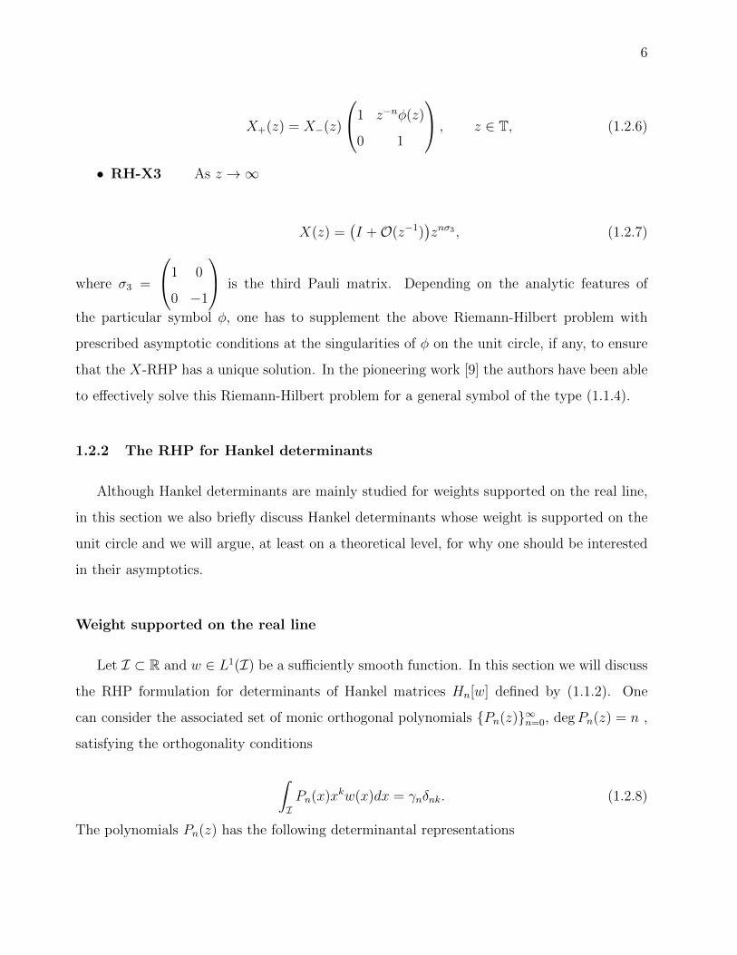
6

X+(z) = X−(z)

1 z−nφ(z)

0 1

, z ∈ T, (1.2.6)

• RH-X3 As z →∞

X(z) =(I +O(z−1)

)znσ3 , (1.2.7)

where σ3 =

1 0

0 −1

is the third Pauli matrix. Depending on the analytic features of

the particular symbol φ, one has to supplement the above Riemann-Hilbert problem with

prescribed asymptotic conditions at the singularities of φ on the unit circle, if any, to ensure

that the X-RHP has a unique solution. In the pioneering work [9] the authors have been able

to effectively solve this Riemann-Hilbert problem for a general symbol of the type (1.1.4).

1.2.2 The RHP for Hankel determinants

Although Hankel determinants are mainly studied for weights supported on the real line,

in this section we also briefly discuss Hankel determinants whose weight is supported on the

unit circle and we will argue, at least on a theoretical level, for why one should be interested

in their asymptotics.

Weight supported on the real line

Let I ⊂ R and w ∈ L1(I) be a sufficiently smooth function. In this section we will discuss

the RHP formulation for determinants of Hankel matrices Hn[w] defined by (1.1.2). One

can consider the associated set of monic orthogonal polynomials Pn(z)∞n=0, degPn(z) = n ,

satisfying the orthogonality conditions

∫IPn(x)xkw(x)dx = γnδnk. (1.2.8)

The polynomials Pn(z) has the following determinantal representations

7

Pn(z) =1

detHn[w]det

w0 w1 · · · wn−1 wn

w1 w2 · · · wn wn+1

......

......

...

wn−1 wn · · · w2n−2 w2n−1

1 z · · · zn−1 zn

, and hence γn =

detHn+1[w]

detHn[w].

(1.2.9)

It is due to Fokas, Its and Kitaev [6] that the following matrix-valued function which is built

from the orthogonal polynomials and the Cauchy transforms of the weight w multiplied by

the orthogonal polynomials

Y (z) =

Pn(z)1

2πi

∫I

Pn(x)w(x)

x− zdx

− 2πi

hn−1

Pn−1(z) − 1

hn−1

∫I

Pn−1(x)w(x)

x− zdx

, (1.2.10)

satisfies the following Riemann-Hilbert problem:

• RH-Y1 Y : C \ [a, b]→ C2×2 is analytic.

• RH-Y2 The limits of Y (z) as z tends to x ∈ I from the upper and lower half plane

exist, and are denoted Y±(x) respectively and are related by

Y+(x) = Y−(x)

1 w(x)

0 1

, x ∈ I. (1.2.11)

• RH-Y3 As z →∞,

Y (z) =(I +O(z−1)

)znσ3 . (1.2.12)

Like what we mentioned about Toeplitz determinants, the analytic properties of w dictates

certain asymptotic conditions on the RHP setting, as z approaches singularities of w which

belong to I. For instance, if w is a modified Jacobi weight w(x) = h(x)(1 − x)α(1 + x)β,

I = [−1, 1], in order to propose a Riemann-Hilbert problem with a unique solution, one has

to specify asymptotic conditions as z → ±1 as well (see [10]). Furthermore, if w has Fisher-

Hartwig singularities at tjmj=1 ⊂ I, one has to augment the above Riemann-Hilbert problem

8

with specific asymptotic conditions as z → tj (see [3]). The above Reiemann-Hilbert problem

can be solved for sufficiently large n via the Deift-Zhou nonlinear steepest descent method,

and hence through integration of associated differential identities, the large-n asymptotics of

detHn[w] can be found (e.g. see [3], [4]).

Weight supported on the unit circle

In this section we will consider the determinants of Hankel matricesHn[w] = wj+k, whose

symbol is supported on the unit circle. We will show that this determinant is, in a natural

way, related to a Toeplitz determinant whose symbol contains the large parameter n, making

its winding number monotonically decrease as n→∞. But first let us recall the situation for

Toeplitz symbols with fixed non-zero winding number. A.Bottcher and H.Widom considered

this problem from an operator-theoretic point of view in [11]. P.Deift, A.Its and I.Krasovsky

in [9] prove yet another remarkable result where they relate the Toeplitz determinant with

symbol z`φ(z), where ` ∈ Z is independent of n, to the Toeplitz determinant with symbol φ

that can be asymptotically analyzed via the RHP method. Here we mention their result:

Lemma 1.2.1 (From [9]) Let the Toeplitz determinants Dn(φ) be nonzero for all n ≥ N0,

for some N0 ∈ N. Let qk(z) = Qk(z)/κk, qk(z) = Qk/κk, k = N0, N0 + 1, · · · be the system of

monic bi-orthogonal polynomials on the unit circle with respect to the weight φ. Fix an integer

` > 0, then if

Fk := det

qk(0) qk+1(0) · · · qk+`−1(0)

ddzqk(0) d

dzqk+1(0) · · · d

dzqk+`−1(0)

......

...

d`−1

dz`−1 qk(0) d`−1

dz`−1 qk+1(0) · · · d`−1

dz`−1 qk+`−1(0)

6= 0, (1.2.13)

for k = N0, N0 + 1, · · · , n− 1, we have

Dn(z`φ(z)) =(−1)`nFn∏`−1

j=1 j!Dn(φ(z)), n ≥ N0. (1.2.14)

9

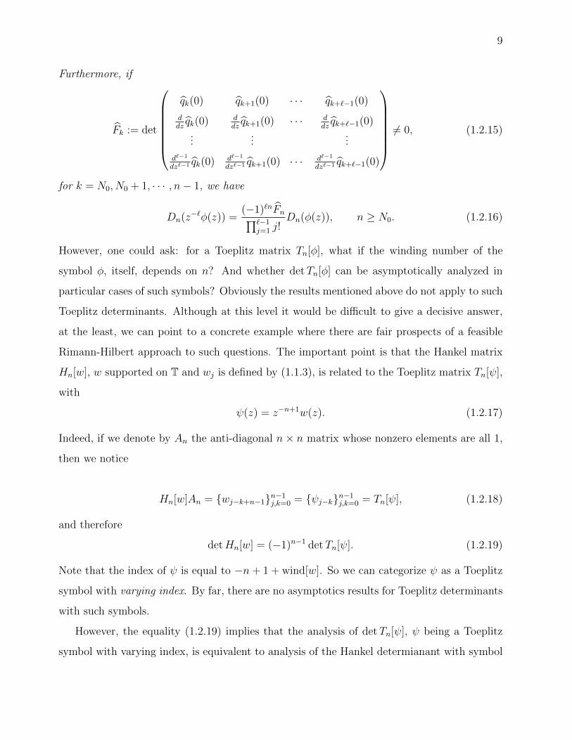
Furthermore, if

Fk := det

qk(0) qk+1(0) · · · qk+`−1(0)

ddzqk(0) d

dzqk+1(0) · · · d

dzqk+`−1(0)

......

...

d`−1

dz`−1 qk(0) d`−1

dz`−1 qk+1(0) · · · d`−1

dz`−1 qk+`−1(0)

6= 0, (1.2.15)

for k = N0, N0 + 1, · · · , n− 1, we have

Dn(z−`φ(z)) =(−1)`nFn∏`−1

j=1 j!Dn(φ(z)), n ≥ N0. (1.2.16)

However, one could ask: for a Toeplitz matrix Tn[φ], what if the winding number of the

symbol φ, itself, depends on n? And whether detTn[φ] can be asymptotically analyzed in

particular cases of such symbols? Obviously the results mentioned above do not apply to such

Toeplitz determinants. Although at this level it would be difficult to give a decisive answer,

at the least, we can point to a concrete example where there are fair prospects of a feasible

Rimann-Hilbert approach to such questions. The important point is that the Hankel matrix

Hn[w], w supported on T and wj is defined by (1.1.3), is related to the Toeplitz matrix Tn[ψ],

with

ψ(z) = z−n+1w(z). (1.2.17)

Indeed, if we denote by An the anti-diagonal n× n matrix whose nonzero elements are all 1,

then we notice

Hn[w]An = wj−k+n−1n−1j,k=0 = ψj−kn−1

j,k=0 = Tn[ψ], (1.2.18)

and therefore

detHn[w] = (−1)n−1 detTn[ψ]. (1.2.19)

Note that the index of ψ is equal to −n+ 1 + wind[w]. So we can categorize ψ as a Toeplitz

symbol with varying index. By far, there are no asymptotics results for Toeplitz determinants

with such symbols.

However, the equality (1.2.19) implies that the analysis of detTn[ψ], ψ being a Toeplitz

symbol with varying index, is equivalent to analysis of the Hankel determianant with symbol

10

w supported on the unit circle. For the former, In the same spirit, we can consider monic

orthogonal polynomials P n(z)∞n=0, deg

P n(z) = n, associated to the weight w satisfying

∫T

P n(z)zkw(z−1)

dz

2πiz=γnδn,k, k = 0, 1, · · · , n. (1.2.20)

The polynomialsP n(z) have the following determinantal representations

P n(z) =

1

detHn[w]det

w0 w1 · · · wn−1 wn

w1 w2 · · · wn wn+1

......

......

...

wn−1 wn · · · w2n−2 w2n−1

1 z · · · zn−1 zn

, and hence

γn =

detHn+1[w]

detHn[w].

(1.2.21)

If we consider the following matrix-valued function which is built from the orthogonal poly-

nomials and their Cauchy transforms

Y (z) =

P n(z)

∫T

P n(ζ)w(ζ−1)

ζ − zdζ

2πiζ

− 1γn−1

P n−1(z) − 1

γn−1

∫T

P n−1(ζ)w(ζ−1)

ζ − zdζ

2πiζ

, (1.2.22)

then,Y (z) satisfies the following Riemann-Hilbert problem:

• RH-Y 1

Y : C \ T→ C2×2 is analytic.

• RH-Y 2 The limits of

Y (ζ) as ζ tends to z ∈ T from the inside and outside of the unit

circle exist, these limiting values are denoted byY ±(z) respectively and are related by

Y +(z) =

Y −(z)

1 z−1w(z−1)

0 1

, z ∈ T. (1.2.23)

• RH-Y 3 As z →∞,

Y (z) =

(I +O(z−1)

)znσ3 . (1.2.24)

11

Note that the main difference between the Riemann-Hilbert problem for Toeplitz determinants

and the Riemann-Hilbert problem for Hankel determinants (with w being supported on T)

is in the 12-element of their jump matrices on the unit circle. If an effective analysis of this

Riemann-Hilbert problem be feasible, then one can get a hold of detTn[ψ], ψ being the symbol

with varying index given by (1.2.17), via (1.2.19).

To this end, the work [12] could be a great starting point at least for weights w holomorphic

inside of the unit circle. Here, we briefly explain this connection. In fact, the polynomialsP

satisfying ∫∂D

P n(z)zkf(z)

dz

2πiz=γnδn,k, k = 0, 1, · · · , n. (1.2.25)

are the denominators of the the diagonal Pade’ approximants, in D, to a function f holo-

morphic at infinity. Here, D is assumed to be a connected domain containing the point at

infinity in which f is holomorphic and single valued. In particular, when f ≡ w(z−1) and

D ≡ C \ D, D being the unit disk, then the orthogonality conditions (1.2.20) and (1.2.25)

are the same, provided that w be analytic inside of the unit circle, which hence implies that

f ≡ w is analytic in D. This means that through the relation (1.2.21), expressing the ratio of

Hankel determinants in terms of the the normsγn of Pade’ approximant denominators, one

can obtain the asymptotics of Hankel determinants using the relevant differential identities as

usual. This would finally provide us with the asymptotics of Toeplitz determinants detTn[ψ]

with varying index.

1.2.3 The RHP for integrable integral operators

In this section we will present a Riemann-Hilbert problem for integrable integral operators

and the corresponding Fredholm determinants. This Riemann-Hilbert problem was first found

by A.Its, A.Izergin, V.Korepin, N.Slavnov in [13]. Let us revisit the kernel Kn(z, λ) defined

by (1.1.7) and the associated integral operator K:

(Ku)(z) :=

∫Σ

Kn(z, λ)u(λ)dλ, with K(z, λ) =fT (z)h(λ)

z − λ, (1.2.26)

12

where f, h : C → CN , and by fj and hj we denote the j-th component of vectors f and g,

respectively. One requires fT (z)h(z) = 0 to avoid singularities on the diagonal of the kernel.

A key property of operators (1.2.26) is that the Resolvent operator R := (1−K)−1 − 1 also

belongs to the class of integrable integral operators, i.e. it can be written as

R(z, λ) =F T (z)H(λ)

z − λ, (1.2.27)

where

Fj = (1−K)−1fj, Hj = (1−KT )−1hj. (1.2.28)

The vector functions F and H can be computed in terms of a certain matrix Riemann-Hilbert

problem. To arrive at this RHP, let us first consider the following N × N matrix-valued

function

Y(z) = I −∫

Σ

F (λ)hT (λ)dλ

λ− z. (1.2.29)

Thus, by the Plemelj-Sokhotskii formula we have

Y+(z)−Y−(z) = −2πiF (z)hT (z), (1.2.30)

Since we have assumed that hT (z)f(z) = 0, we get

Y+(z)f(z) = Y−(z)f(z). (1.2.31)

Also, since hT (λ)f(z) = fT (z)h(λ) is a scalar, we have

F (λ)hT (λ)f(z) = fT (z)h(λ)F (λ). (1.2.32)

Using this, (1.2.29) and (1.2.31) we have

Y±(z)f(z) = f(z)−∫

Σ

F (λ)hT (λ)f(z)dλ

λ− z= f(z)−

∫Σ

fT (z)h(λ)F (λ)dλ

λ− z

= f(z) +

∫Σ

K(z, λ)F (λ)dλ.

(1.2.33)

Therefore

(KF )(z) = Y±(z)f(z)− f(z). (1.2.34)

13

Note that by definition of F

(KF )(z) = F (z)− f(z),

and hence

F (z) = Y±(z)f(z). (1.2.35)

In a similar fashion, we can show that

H(z) = (YT±)−1(z)h(z). (1.2.36)

Note that (1.2.30) and (1.2.35) together imply that

Y−(z) = Y+(z)(I + 2πif(z)hT (z)

). (1.2.37)

This equation, supplemented by the analytic properties of the Cauchy integral, show that

Y(z) solves the following N ×N matrix Riemann-Hilbert problem:

• RH-Y1 Y : C \ Σ→ CN×N is analytic.

• RH-Y2 The limits of Y(ζ) as ζ tends to z ∈ Σ along any non-tangential path exist,

and are denoted by Y±(z) naturally w.r.t. the orientation of Σ. These limiting values

are related by

Y−(z) = Y+(z)JY(z), z ∈ Σ. (1.2.38)

• RH-Y3 As z →∞, we have Y(z) = I +O(z−1).

In the standard way, one can show that the solution to this Riemann-Hilbert problem, if

exists, is unique. Thus, if the solution Y of this RHP can be found, then F , H and R could

be found as well via (1.2.35), (1.2.36), and (1.2.27), respectively.

14

2. ASYMPTOTICS OF HANKEL DETERMINANTS WITH A

LAGUERRE-TYPE OR JACOBI-TYPE POTENTIAL AND

FISHER-HARTWIG SINGULARITIES

Abstract.

We obtain large n asymptotics of n × n Hankel determinants whose weight has a one-

cut regular potential and Fisher-Hartwig singularities. We restrict our attention to the case

where the associated equilibrium measure possesses either one soft edge and one hard edge

(Laguerre-type) or two hard edges (Jacobi-type). We also present some applications in the

theory of random matrices. In particular, we can deduce from our results asymptotics for

partition functions with singularities, central limit theorems, correlations of the characteristic

polynomials, and gap probabilities for (piecewise constant) thinned Laguerre and Jacobi-

type ensembles. Finally, we mention some links with the topics of rigidity and Gaussian

multiplicative chaos. This is a joint work with C. Charlier.

2.1 Introduction

Hankel determinants with Fisher-Hartwig (FH) singularities appear naturally in random

matrix theory. Among others, they can express correlations of the characteristic polynomial

of a random matrix, or gap probabilities in the point process of the thinned spectrum, see

e.g. the introductions of [3,4,9] for more details. In these applications, the size n of an n× n

Hankel determinant is equal to the size of the underlying n × n random matrices. Large

n asymptotics for such determinants have already been widely studied, see e.g. [3–5, 14, 15].

Recent developments in the theory of Gaussian multiplicative chaos [15] provide a renewed

interest in these asymptotics. For example, such asymptotics provide crucial estimates in the

study of rigidity of eigenvalues of a random matrix [16].

15

In the present work, we restrict our attention on large n asymptotics of Hankel determinants

det

(∫Ixj+kw(x)dx

)j,k=0,...,n−1

, (2.1.1)

whose weight w is supported on an interval I ⊂ R, and is of the form

w(x) = e−nV (x)eW (x)ω(x). (2.1.2)

The function W is continuous on I and ω contains the FH singularities (they will be described

in more details below). The potential V is real analytic on I and, in case I is unbounded,

satisfies limx→±∞,x∈I V (x)/ log |x| = +∞. Furthermore, we assume that V is one-cut and

regular. These properties are described in terms of the equilibrium measure µV , which is the

unique minimizer of the functional∫∫log |x− y|−1dµ(x)dµ(y) +

∫V (x)dµ(x) (2.1.3)

among all Borel probability measures µ on I. One-cut means that the support of µV consists

of a single interval. For convenience, and without loss of generality, we will assume that this

interval is [−1, 1]. It is known that µV is completely characterized by the Euler-Lagrange

variational conditions

2

∫ 1

−1

log |x− s|dµV (s) = V (x)− `, for x ∈ [−1, 1], (2.1.4)

2

∫ 1

−1

log |x− s|dµV (s) ≤ V (x)− `, for x ∈ I \ [−1, 1], (2.1.5)

where ` ∈ R is a constant. Regular means that the Euler-Lagrange inequality (2.1.5) is strict

on I \ [−1, 1], and that the density of the equilibrium measure is positive on (−1, 1). The

three canonical cases are the following:

1. I = R and dµV (x) = ψ(x)√

1− x2dx,

2. I = [−1,∞) and dµV (x) = ψ(x)√

1−x1+x

dx,

3. I = [−1, 1] and dµV (x) = ψ(x) 1√1−x2dx,

where ψ is real analytic on I, such that ψ(x) > 0 for all x ∈ [−1, 1]. We will refer to these three

cases as Gaussian-type, Laguerre-type and Jacobi-type weights, respectively. Note that (2.1.5)

16

is automatically satisfied for Jacobi-type weights, since I = [−1, 1]. Well-known examples for

potentials of such weights are

1. V (x) = 2x2 for Gaussian-type weight, with ` = 1 + 2 log 2 and ψ(x) = 2π,

2. V (x) = 2(x+ 1) for Laguerre-type weight, with ` = 2 + 2 log 2 and ψ(x) = 1π,

3. V (x) = 0 for Jacobi-type weight, with ` = 2 log 2 and ψ(x) = 1π.

In the language of random matrix theory, the interval (−1, 1) is called the bulk, and ±1 are

the edges. An edge is said to be “soft” if there can be eigenvalues beyond it, and “hard” if

this is impossible. On the level of the equilibrium measure, a soft edge translates into a square

root vanishing of dµVdx

, while a hard edge means that dµVdx

blows up like an inverse square root.

Thus, there are two soft edges at ±1 for Gaussian-type weights, one hard edge at −1 and one

soft edge at 1 for Laguerre-type weights, and two hard edges for Jacobi-type weights.

The function ω that appears in (2.1.2) is defined by

ω(x) =m∏j=1

ωαj(x)ωβj(x)×

1, for Gaussian-type weights,

(x+ 1)α0 , for Laguerre-type weights,

(x+ 1)α0(1− x)αm+1 , for Jacobi-type weights,

(2.1.6)

where

ωαk(x) = |x− tk|αk , ωβk(x) =

eiπβk , if x < tk,

e−iπβk , if x > tk,(2.1.7)

with

−1 < t1 < . . . < tm < 1. (2.1.8)

The functions ωαk and ωβk represent the root-type and jump-type singularities at tk, respec-

tively. These singularities are named after Fisher and Hartwig, due to their pioneering work

in their identification [1]. Since ωβk+1 = −ωβk , we can assume without loss of generality

that <βk ∈ (−12, 1

2] for all k. Finally, to ensure integrability of the weight (at least for suf-

ficiently large n), we require that <αk > −1 for all k and, in case I is unbounded, that

W (x) = O(V (x)) as x→ ±∞, x ∈ I.

17

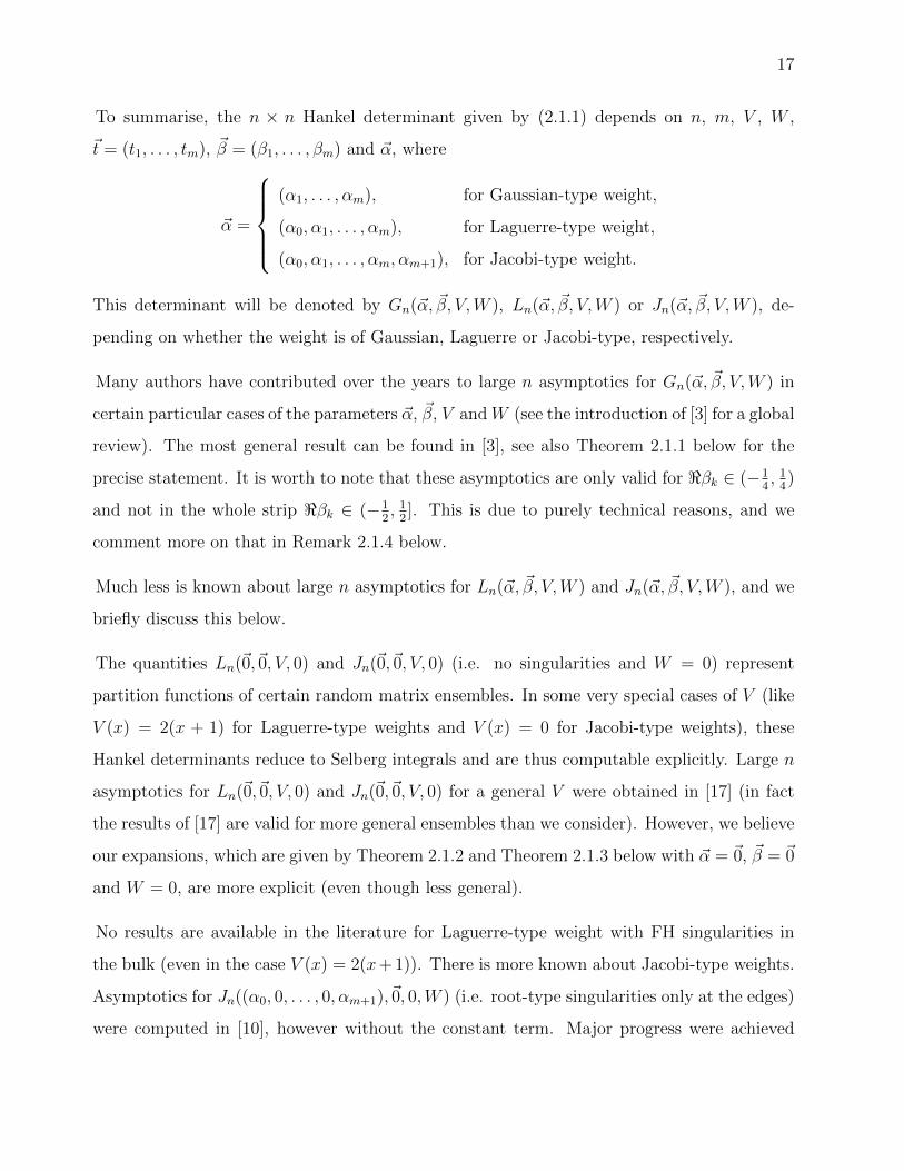
To summarise, the n × n Hankel determinant given by (2.1.1) depends on n, m, V , W ,

~t = (t1, . . . , tm), ~β = (β1, . . . , βm) and ~α, where

~α =

(α1, . . . , αm), for Gaussian-type weight,

(α0, α1, . . . , αm), for Laguerre-type weight,

(α0, α1, . . . , αm, αm+1), for Jacobi-type weight.

This determinant will be denoted by Gn(~α, ~β, V,W ), Ln(~α, ~β, V,W ) or Jn(~α, ~β, V,W ), de-

pending on whether the weight is of Gaussian, Laguerre or Jacobi-type, respectively.

Many authors have contributed over the years to large n asymptotics for Gn(~α, ~β, V,W ) in

certain particular cases of the parameters ~α, ~β, V andW (see the introduction of [3] for a global

review). The most general result can be found in [3], see also Theorem 2.1.1 below for the

precise statement. It is worth to note that these asymptotics are only valid for <βk ∈ (−14, 1

4)

and not in the whole strip <βk ∈ (−12, 1

2]. This is due to purely technical reasons, and we

comment more on that in Remark 2.1.4 below.

Much less is known about large n asymptotics for Ln(~α, ~β, V,W ) and Jn(~α, ~β, V,W ), and we

briefly discuss this below.

The quantities Ln(~0,~0, V, 0) and Jn(~0,~0, V, 0) (i.e. no singularities and W = 0) represent

partition functions of certain random matrix ensembles. In some very special cases of V (like

V (x) = 2(x + 1) for Laguerre-type weights and V (x) = 0 for Jacobi-type weights), these

Hankel determinants reduce to Selberg integrals and are thus computable explicitly. Large n

asymptotics for Ln(~0,~0, V, 0) and Jn(~0,~0, V, 0) for a general V were obtained in [17] (in fact

the results of [17] are valid for more general ensembles than we consider). However, we believe

our expansions, which are given by Theorem 2.1.2 and Theorem 2.1.3 below with ~α = ~0, ~β = ~0

and W = 0, are more explicit (even though less general).

No results are available in the literature for Laguerre-type weight with FH singularities in

the bulk (even in the case V (x) = 2(x+ 1)). There is more known about Jacobi-type weights.

Asymptotics for Jn((α0, 0, . . . , 0, αm+1),~0, 0,W ) (i.e. root-type singularities only at the edges)

were computed in [10], however without the constant term. Major progress were achieved

18

in [9, 14], in which the authors derived large n asymptotics for Jn(~α, ~β, 0,W ) including the

constant term (under very weak assumption on W , and for general value of ~β such that

<βk ∈ (−12, 1

2]).

The goal of the present paper is to fill a gap in the literature on large n asymptotics of Hankel

determinants with a one-cut potential and FH singularities. In Theorem 2.1.2 and Theorem

2.1.3 below, we find large n asymptotics for Ln(~α, ~β, V,W ) and Jn(~α, ~β, V,W ) including the

constant term. First, we rewrite (in a slightly different way) the result of [3] in Theorem 2.1.1

for the reader’s convenience, in order to ease the comparison between the three canonical

types of weights.

Theorem 2.1.1 (from [3] for Gaussian-type weight)

Let m ∈ N, and let tj, αj and βj be such that

−1 < t1 < . . . < tm < 1, and <αj > −1, <βj ∈ (−14, 1

4) for j = 1, . . . ,m.

Let V be a one-cut regular potential whose equilibrium measure is supported on [−1, 1] with

density ψ(x)√

1− x2, and let W : R → R be analytic in a neighbourhood of [−1, 1], locally

Holder-continuous on R and such that W (x) = O(V (x)), as |x| → ∞. As n→∞, we have

Gn(~α, ~β, V,W ) = exp

(C1n

2 + C2n+ C3 log n+ C4 +O( log n

n1−4βmax

)), (2.1.9)

with βmax = max|<β1|, . . . , |<βm| and

C1 = − log 2− 3

4− 1

2

∫ 1

−1

(V (x)− 2x2)

(2

π+ ψ(x)

)√1− x2dx, (2.1.10)

C2 = log(2π)−A log 2− A2π

∫ 1

−1

V (x)− 2x2

√1− x2

dx+

∫ 1

−1

W (x)ψ(x)√

1− x2dx (2.1.11)

+m∑j=1

αj2

(V (tj)− 1) +m∑j=1

πiβj

(1− 2

∫ 1

tj

ψ(x)√

1− x2dx

),

C3 = − 1

12+

m∑j=1

(α2j

4− β2

j

), (2.1.12)

19

C4 = ζ ′(−1)− 1

24log(π

2ψ(−1)

)− 1

24log(π

2ψ(1)

)+

m∑j=1

(α2j

4− β2

j

)log(π

2ψ(tj)

)+

∑1≤j<k≤m

[log

((1− tjtk −

√(1− t2j)(1− t2k)

)2βjβk

2αjαk

2 |tj − tk|αjαk

2+2βjβk

)+iπ

2(αkβj − αjβk)

]

+m∑j=1

(α2j

4log(2√

1− t2j)− β2

j log(

8(1− t2j)3/2))

+Am∑j=1

iβj arcsin tj

+m∑j=1

logG(1 +

αj2

+ βj)G(1 +αj2− βj)

G(1 + αj)(2.1.13)

+A2π

∫ 1

−1

W (x)√1− x2

dx−m∑j=1

αj2W (tj) +

m∑j=1

iβjπ

√1− t2j−

∫ 1

−1

W (x)√1− x2(tj − x)

dx

+1

4π2

∫ 1

−1

W (x)√1− x2

(−∫ 1

−1

W ′(y)√

1− y2

x− ydy

)dx,

where G is Barnes’ G-function, ζ is Riemann’s zeta-function, where we use the notations −∫

for the Cauchy principal value integral, and

A =m∑j=1

αj. (2.1.14)

Furthermore, the error term in (2.1.9) is uniform for all αk in compact subsets of

z ∈ C : <z > −1, for all βk in compact subsets of z ∈ C : <z ∈(−1

4, 1

4

), and uniform in

t1, . . . , tm, as long as there exists δ > 0 independent of n such that

minj 6=k|tj − tk|, |tj − 1|, |tj + 1| ≥ δ. (2.1.15)

Theorem 2.1.2 (for Laguerre-type weight)

Let m ∈ N, and let tj, αj and βj be such that

−1 = t0 < t1 < . . . < tm < 1, and <αj > −1, <βj ∈ (−14, 1

4) for j = 0, . . . ,m,

with β0 = 0. Let V be a one-cut regular potential whose equilibrium measure is supported on

[−1, 1] with density ψ(x)√

1−x1+x

, and let W : R+ → R be analytic in a neighbourhood of [−1, 1],

locally Holder-continuous on R+ and such that W (x) = O(V (x)), as x → +∞. As n → ∞,

we have

Ln(~α, ~β, V,W ) = exp

(C1n

2 + C2n+ C3 log n+ C4 +O( log n

n1−4βmax

)), (2.1.16)

20

with βmax = max|<β1|, . . . , |<βm| and

C1 = − log 2− 3

2− 1

2

∫ 1

−1

(V (x)− 2(x+ 1))

(1

π+ ψ(x)

)√1− x1 + x

dx, (2.1.17)

C2 = log(2π)−A log 2− A2π

∫ 1

−1

V (x)− 2(x+ 1)√1− x2

dx+

∫ 1

−1

W (x)ψ(x)

√1− x1 + x

dx (2.1.18)

+m∑j=0

αj2

(V (tj)− 2) +m∑j=1

πiβj

(1− 2

∫ 1

tj

ψ(x)

√1− x1 + x

dx

),

C3 = −1

6+α2

0

2+

m∑j=1

(α2j

4− β2

j

), (2.1.19)

C4 = 2ζ ′(−1)− 1− 4α20

8log (πψ(−1))− 1

24log (πψ(1)) +

m∑j=1

(α2j

4− β2

j

)log (πψ(tj))

+α0

2log(2π) +

∑0≤j<k≤m

[log

((1− tjtk −

√(1− t2j)(1− t2k)

)2βjβk

2αjαk

2 |tj − tk|αjαk

2+2βjβk

)+iπ

2(αkβj − αjβk)

]

+m∑j=1

(α2j

4log

√1− tj1 + tj

− β2j log

(4(1− tj)3/2(1 + tj)

1/2))

+Am∑j=1

iβj arcsin tj

− logG(1 + α0) +m∑j=1

logG(1 +

αj2

+ βj)G(1 +αj2− βj)

G(1 + αj)(2.1.20)

+A2π

∫ 1

−1

W (x)√1− x2

dx−m∑j=0

αj2W (tj) +

m∑j=1

iβjπ

√1− t2j−

∫ 1

−1

W (x)√1− x2(tj − x)

dx

+1

4π2

∫ 1

−1

W (x)√1− x2

(−∫ 1

−1

W ′(y)√

1− y2

x− ydy

)dx,

where G is Barnes’ G-function, ζ is Riemann’s zeta-function, where we use the notations −∫

for the Cauchy principal value integral, and

A =m∑j=0

αj. (2.1.21)

Furthermore, the error term in (2.1.16) is uniform for all αk in compact subsets of

z ∈ C : <z > −1, for all βk in compact subsets of z ∈ C : <z ∈(−1

4, 1

4

), and uniform in

t1, . . . , tm, as long as there exists δ > 0 independent of n such that

minj 6=k|tj − tk|, |tj − 1|, |tj + 1| ≥ δ. (2.1.22)

21

Theorem 2.1.3 (for Jacobi-type weight)

Let m ∈ N, and let tj, αj and βj be such that

−1 = t0 < t1 < . . . < tm < tm+1 = 1, and <αj > −1, <βj ∈ (−14, 1

4) for j = 0, . . . ,m+1,

with β0 = 0 = βm+1. Let V be a one-cut regular potential whose equilibrium measure is

supported on [−1, 1] with density ψ(x)√1−x2 , and let W : [−1, 1]→ R be analytic in a neighbourhood

of [−1, 1].

As n→∞, we have

Jn(~α, ~β, V,W ) = exp

(C1n

2 + C2n+ C3 log n+ C4 +O( log n

n1−4βmax

)), (2.1.23)

with βmax = max|<β1|, . . . , |<βm| and

C1 = − log 2− 1

2

∫ 1

−1

V (x)

(1

π+ ψ(x)

)dx√

1− x2, (2.1.24)

C2 = log(2π)−A log 2− A2π

∫ 1

−1

V (x)√1− x2

dx+

∫ 1

−1

W (x)ψ(x)√1− x2

dx (2.1.25)

+m+1∑j=0

αj2V (tj) +

m∑j=1

πiβj

(1− 2

∫ 1

tj

ψ(x)√1− x2

dx

),

C3 = −1

4+α2

0 + α2m+1

2+

m∑j=1

(α2j

4− β2

j

), (2.1.26)

C4 = 3ζ ′(−1) +log 2

12− 1−4α2

0

8log (πψ(−1))−

1−4α2m+1

8log (πψ(1)) +

m∑j=1

(α2j

4− β2

j

)log (πψ(tj))

+α0 + αm+1

2log(2π) +

∑0≤j<k≤m+1

[log

((1− tjtk −

√(1− t2j)(1− t2k)

)2βjβk

2αjαk

2 |tj − tk|αjαk

2+2βjβk

)+iπ

2(αkβj − αjβk)

]

+m∑j=1

(α2j

4log

1√1− t2j

− β2j log

(4√

1− t2j))

+Am∑j=1

iβj arcsin tj −α2

0 + α2m+1

2log 2

− logG(1 + α0)− logG(1 + αm+1) +m∑j=1

logG(1 +

αj2

+ βj)G(1 +αj2− βj)

G(1 + αj)(2.1.27)

+A2π

∫ 1

−1

W (x)√1− x2

dx−m+1∑j=0

αj2W (tj) +

m∑j=1

iβjπ

√1− t2j−

∫ 1

−1

W (x)√1− x2(tj − x)

dx

+1

4π2

∫ 1

−1

W (x)√1− x2

(−∫ 1

−1

W ′(y)√

1− y2

x− ydy

)dx,

22

where G is Barnes’ G-function, ζ is Riemann’s zeta-function, where we use the notations −∫

for the Cauchy principal value integral, and

A =m+1∑j=0

αj. (2.1.28)

Furthermore, the error term in (2.1.23) is uniform for all αk in compact subsets of

z ∈ C : <z > −1, for all βk in compact subsets of z ∈ C : <z ∈(−1

4, 1

4

), and uniform in

t1, . . . , tm, as long as there exists δ > 0 independent of n such that

minj 6=k|tj − tk|, |tj − 1|, |tj + 1| ≥ δ. (2.1.29)

Remark 2.1.4 The assumption <βk ∈ (−14, 1

4) comes from some technicalities in our analy-

sis. Similar difficulties were encountered in [5] for Gn(0, ~β, 2x2, 0) with m = 1 (i.e. ~β = β1),

and in [14] for Jn(~α, ~β, 0,W ). In [14], the authors overcame these technicalities, and were

able to extend their results from <βk ∈ (−14, 1

4) to <βk ∈ (−1

2, 1

2) by using Vitali’s theorem.

Their argument relies crucially on w being independent of n (which is true only for Jacobi-

type weights with V = 0) and can not be adapted straightforwardly to the situation of Theorem

2.1.1, 2.1.2 and 2.1.3. However, the method presented in this paper allows in principle, but

with significant extra effort, to obtain asymptotics for the whole region <βk ∈ (−12, 1

2). Fi-

nally, extending the result from <βk ∈ (−12, 1

2) to <βk ∈ (−1

2, 1

2] would rely on so-called FH

representations of the weight, see [9] for more details.

Remark 2.1.5 Starting with a function f defined on the unit circle, the associated Toeplitz

determinant is given by

det

(1

2π

∫ π

−πf(eiθ)e−i(j−k)θdθ

)j,k=0,...,n−1

. (2.1.30)

Asymptotics of large Toeplitz determinants is another topic of high interest, which presents

applications similar to those of Hankel determinants, but for point processes defined on the

unit circle instead of the real line. In [9], the authors obtained first large n asymptotics

for certain Toeplitz determinants (with the zero potential), and deduced from them large n

asymptotics for Jn(~α, ~β, 0,W ). It is therefore natural to wonder if one can translate the

23

results of Theorem 2.1.1, 2.1.2 and 2.1.3 into asymptotics for Toeplitz determinants with a

one-cut regular potential. We explain here why we believe this is not obvious.

The main tool used in [9] is a relation of Szego [18] . If

f(eiθ) = w(cos θ)| sin θ|, (2.1.31)

we can express orthogonal polynomials on the unit circle associated to f in terms of orthogonal

polynomials on the real line associated to w. Note that this transformation can only work in

all generality from Toeplitz to Hankel, and not the other way around. Indeed, the weight

w can be arbitrary, but the function f is of a very particular type (in particular it satisfies

f(eiθ) = f(e−iθ)).

We also believe that asymptotics for Toeplitz determinants with a one-cut regular potential

and FH singularities would not imply Theorem 2.1.1, 2.1.2 and 2.1.3 (with the exception of

V = 0 for Jacobi-type weights as done in [9]). The main reason is that, as shown from the

change of variables s = cos θ in (2.1.4), the potential V on the unit circle is related to the

potential V on the interval [−1, 1] via the relation V (eiθ) = V (cos θ), which means that at least

one potential is not analytic (except if V is a constant as in [9]). Finally, we also point out

that regarding e.g. Gaussian-type weights, again the change of variables s = cos θ in (2.1.4)

shows that the associated equilibrium measure µV on the unit circle vanishes as a square at

θ = 0 and θ = π, which is not a “regular” weight. To avoid this problem, one could by a

simple change of variables shrink the support of µV into [−a, a] with 0 < a < 1, but then µV

would be supported on two disjoint intervals.

Applications

In this section, we provide several applications of Theorem 2.1.1, Theorem 2.1.2 and The-

orem 2.1.3 in random matrix theory. For each type of weight, there corresponds a particu-

lar type of matrix ensemble. Assume that V is a Gaussian-type potential. The associated

24

Gaussian-type matrix ensemble consists of the space of n × n complex Hermitian matrices

endowed with the probability measure

1

ZGn

e−nTr(V (M))dM, dM =n∏i=1

dMii

∏1≤i<j≤n

d<Mijd=Mij, (2.1.32)

with ZGn the normalizing constant. Laguerre-type matrix ensembles are usually defined on

n×n complex positive definite Hermitian matrices. Here we instead assume, for Laguerre-type

matrix ensembles, that all matrices have eigenvalues geater than −1 (this assumption eases

the comparison between the three cases). Such ensembles have a probability measure of the

form1

ZLn

det(I +M)α0e−nTr(V (M))dM, α0 > −1, (2.1.33)

where V is of Laguerre-type, and ZLn is the normalizing constant. Finally, a Jacobi-type

matrix ensemble consists of the space of n × n Hermitian matrices whose spectrum lies the

interval [−1, 1], with a probability measure of the form

1

ZJn

det(I +M)α0 det(I −M)αm+1e−nTr(V (M))dM, α0, αm+1 > −1, (2.1.34)

with a Jacobi-type potential V and ZJn is again the normalizing constant. These three types of

matrix ensembles are invariant under unitary conjugation and induce the following probability

measures on the eigenvalues x1, . . . , xn:

1

ZGn

∏1≤j<k≤n

(xk − xj)2

n∏j=1

e−nV (xj)dxj, x1, . . . , xn ∈ R, (2.1.35)

1

ZLn

∏1≤j<k≤n

(xk − xj)2

n∏j=1

(1 + xj)α0e−nV (xj)dxj, x1, . . . , xn ∈ [−1,∞), (2.1.36)

1

ZJn

∏1≤j<k≤n

(xk − xj)2

n∏j=1

(1 + xj)α0(1− xj)αm+1e−nV (xj)dxj, x1, . . . , xn ∈ [−1, 1], (2.1.37)

where the first, second and third line read for Gaussian, Laguerre, and Jacobi-type matrix

ensembles, respectively, and ZGn , ZL

n and ZJn are the normalizing constants, also called the

partition functions.

25

Partition function asymptotics in the one-cut regime. By Heine’s formula, the parti-

tion functions can be rewritten as Hankel determinants of the form (2.1.1) with W = 0, ~β = ~0

and α1 = ... = αm = 0 and can thus be deduced from theorems 2.1.1, 2.1.2 and 2.1.3. Large

n asymptotics for ZGn have been obtained in some particular cases of V in [19, 20] using RH

methods. Then large n asymptotics for ZGn , ZL

n and ZJn were all obtained in [17] using loop

equations, however these asymptotics are valid only without singularities, i.e. only for α0 = 0

for ZLn and only for α0 = αm+1 = 0 for ZJ

n . Finally, via RH methods, large n asymptotics for

ZGn have been obtained only recently in [15] for general potential V .

Corollary 2.1.5.1 As n→ +∞, we have

ZGn = exp

(−(

log 2 +3

4+

1

2

∫ 1

−1

(V (x)− 2x2)( 2

π+ ψ(x)

)√1− x2dx

)n2 (2.1.38)

+ log(2π)n− 1

12log n+ ζ ′(−1)− 1

24log(π

2ψ(−1)

)− 1

24log(π

2ψ(1)

)+O

( log n

n

)),

ZLn = exp

(−(

log 2 +3

2+

1

2

∫ 1

−1

(V (x)− 2(x+ 1))( 1

π+ ψ(x)

)√1− x1 + x

dx

)n2 (2.1.39)

+

(log(2π)− α0 log 2− α0

2π

∫ 1

−1

V (x)− 2(x+ 1)√1− x2

dx+α0

2(V (−1)− 2)

)n+

(α20

2− 1

6

)log n

+ 2ζ ′(−1)− 1−4α20

8log(πψ(−1)

)− 1

24log(πψ(1) +

α0

2log(2π)− logG(1 + α0) +O

( log n

n

)),

ZJn = exp

(−(

log 2 +1

2

∫ 1

−1

V (x)( 1

π+ ψ(x)

) dx√1− x2

)n2 (2.1.40)

+

(log(2π)− (α0 + αm+1) log 2− α0 + αm+1

2π

∫ 1

−1

V (x)√1− x2

dx+α0

2V (−1) +

αm+1

2V (1)

)n

+

(− 1

4+α2

0 + α2m+1

2

)log n+ 3ζ ′(−1) +

log 2

12− 1−4α2

0

8log (πψ(−1))−

1−4α2m+1

8log (πψ(1))

+α0 + αm+1

2log(2π)− (α0 + αm+1)2

2log 2− log

(G(1 + α0)G(1 + αm+1)

)+O

( log n

n

)).

Central limit theorems (CLTs). The function W allows to obtain information about

the global fluctuation properties of the spectrum around the equilibrium measure. In [21],

Johansson obtained a CLT for Gaussian-type ensembles (and is reproduced in (2.1.41) below

for convenience). Until now, there were no CLTs in the literature for Laguerre and Jacobi-type

26

ensembles. These CLTs are obtained in Corollary 2.1.5.2 below, as a rather straightforward

consequence of Theorem 2.1.2 and Theorem 2.1.3.

Corollary 2.1.5.2 (a) Let x1, . . . , xn be distributed according to (2.1.35) and V and W be as

in Theorem 2.1.1. As n→ +∞, we have

n∑i=1

W (xi)− n∫ 1

−1

W (x)ψ(x)√

1− x2dxd−→ N (0, σ2), (2.1.41)

whered−→ means convergence in distribution, and N (0, σ2) is a zero-mean normal random

variable with variance given by

σ2 =1

2π2

∫ 1

−1

W (x)√1− x2

(−∫ 1

−1

W ′(y)√

1− y2

x− ydy

)dx. (2.1.42)

(b) Let x1, . . . , xn be distributed according to (2.1.36) and V and W be as in Theorem 2.1.2.

As n→ +∞, we have

n∑i=1

W (xi)− n∫ 1

−1

W (x)ψ(x)

√1− x1 + x

dxd−→ N (µL, σ

2), (2.1.43)

where σ2 is given by (2.1.42) and the mean µL is given by

µL =α0

2π

∫ 1

−1

W (x)√1− x2

dx− α0

2W (−1). (2.1.44)

(c) Let x1, . . . , xn be distributed according to (2.1.37) and V and W be as in Theorem 2.1.3.

As n→ +∞, we have

n∑i=1

W (xi)− n∫ 1

−1

W (x)ψ(x)√1− x2

dxd−→ N (µJ , σ

2), (2.1.45)

where σ2 is given by (2.1.42) and the mean µJ is given by

µJ =α0 + αm+1

2π

∫ 1

−1

W (x)√1− x2

dx− α0

2W (−1)− αm+1

2W (1). (2.1.46)

Proof We only prove the result for Jacobi-type ensembles. The proofs for the other cases

are similar. From Heine’s formula, we have

EJ[et

∑nj=1W (xj)

]=Jn((α0, 0, ..., 0, αm+1),~0, V, tW

)Jn((α0, 0, ..., 0, αm+1),~0, V, 0

) , t ∈ R, (2.1.47)

27

where EJ means that the expectation is taken with respect to (2.1.37). Let Xn be the random

variable defined by

Xn =n∑j=1

W (xj)− n∫ 1

−1

W (x)ψ(x)√1− x2

dx. (2.1.48)

Theorem 2.1.3 then implies

EJ[etXn

]= exp

(tµJ +

t2

2σ2 +O

( log n

n

)), as n→ +∞. (2.1.49)

Thus, for each t ∈ R, (Xn) is a sequence of random variables whose moment generating func-

tions converge to etµJ+ t2

2σ2

as n→ +∞ (the convergence is pointwise in t ∈ R). Convergence

in distribution follows from well-known convergence theorems (see e.g. [22]).

Correlations of the characteristic polynomials. Let pn(t) =∏n

j=1(t−xj) be the charac-

teristic polynomial associated to a matrix from a Gaussian-type, Laguerre-type or Jacobi-type

ensemble. Supported by numerical evidence, numerous conjectures in the literature have been

formulated about links between pn(t) and the behavior of the Riemann ζ-functions along the

critical line (see e.g. [23]). For Gaussian-type ensembles, correlations with root-type singu-

larities were studied in [4] for V (x) = 2x2 and in [15] for general V . Large n asymptotics

for more general correlations with both root-type and jump-type singularities were obtained

in [3]. However, the cases of Laguerre or Jacobi-type ensembles were still open. In the same

way as noticed in [3, equation (1.16)], we can express these correlations in terms of Hankel

determinants with FH singularities as follows1:

ED[ m∏k=1

|pn(tk)|αke2iβk arg pn(tk)

]=Dn(~α, ~β, V, 0)

ZDn

m∏k=1

e−inπβk , D = G,L, J, (2.1.50)

where EG, EL and EJ are the expectations taken with respect to (2.1.35), (2.1.36) and (2.1.37),

respectively, and where

arg pn(t) =n∑j=1

arg(t− xj), with arg(t− xj) =

0, if xj < t,

−π, if xj > t.(2.1.51)

1There is a n missing in [3, equations (1.16) and (1.22)]: e−iπβk should instead be e−inπβk and s1/2k should

instead be sn/2k . The correct expressions are given by (2.1.50) and (2.1.52) of the present work.

28

Therefore, as an immediate corollary of Theorem 2.1.2 and Theorem 2.1.3, we obtain large n

asymptotics for the correlations given in (2.1.50) for Laguerre and Jacobi-type ensembles.

Gap probabilities in piecewise constant thinned point processes. Given a point

process, a constant thinning consists of removing each point independently with a certain

probability s ∈ [0, 1]. The remaining points, denoted by y1, . . . , yN , form a thinned point pro-

cess, and can be interpreted in certain applications as observed points [24, 25]. Probabilities

of observing a large gap in the thinned sine point process, as well as for thinned eigenvalues

of Haar distributed unitary matrices, have been studied in [26] and [27], respectively. A more

general operation consists of applying a piecewise constant thinning, and was first considered

in [3] for Gaussian-type ensembles. Large gap asymptotics for the piecewise constant thinned

Airy and Bessel point processes were obtained recently in [28] and [29], respectively. From The-

orem 2.1.2 and Theorem 2.1.3, we can deduce large gap asymptotics for (piecewise constant)

thinned Laguerre and Jacobi-type ensembles. Following [3], we consider K ⊆ 1, ...,m + 1.

For each k ∈ K, we remove each point on (tk−1, tk) with a probability sk ∈ (0, 1]. In the same

way as shown in [3, equations (1.20)–(1.22)], we can express gap probabilities in the piecewise

thinned spectrum of Gaussian, Laguerre and Jacobi-type ensembles as follows:

PD(]yj ∈

⋃k∈K

(tk−1, tk) = 0)

=Dn(~α, ~β, V, 0)

ZDn

∏k∈K

sn/2k , D = G,L, J, (2.1.52)

with α1 = ... = αm = 0 and ~β = (β1, ..., βm) given by

2iπβj = log

(sjsj+1

), sj =

sj, if j ∈ K,

1, if j /∈ K,(2.1.53)

and where again PG, PL and PJ are probabilities taken with respect to (2.1.35), (2.1.36) and

(2.1.37), respectively.

Rigidity and Gaussian multiplicative chaos. Let us consider a sequence of matrices Mn

taken from either Gaussian, Laguerre, or Jacobi-type ensembles. As n→ +∞, the logarithm

of the characteristic polynomial of Mn behaves like a log-correlated field. A fundamental tool

in describing some properties of the limiting field is a class of random measures, known as

29

Gaussian multiplicative chaos measures. Roughly speaking, these measures are exponential

of the field, however a precise definition is rather subtle. This subject was introduced by

Kahane in [30], and we refer to [31] for a recent review. For Gaussian-type ensembles, it is

known (from [15]) that a sufficiently small power of the absolute value of the characteristic

polynomial converges weakly in distribution to a Gaussian multiplicative chaos measure. Large

n asymptotics for Hankel determinants with root-type singularities provide crucial estimates in

the proof. Theorem 2.1.2 and Theorem 2.1.3 provide similar estimates for Laguerre and Jacobi-

type ensembles, which could probably be used to prove analogous results for the Laguerre and

Jacobi cases. Another related topic is the study of rigidity, which attempts to answer the

question: “How much can the eigenvalues of a random matrix fluctuate?”. For Gaussian-

type ensembles, this question has been answered in [16]. This time, it is large n asymptotics

for Hankel determinants with jump-type singularities that are crucial in the analysis. In

particular, the proof of [16] relies heavily on Theorem 2.1.1 (with ~α = ~0). Theorem 2.1.2 and

Theorem 2.1.3 provide similar estimates for Laguerre and Jacobi-type ensembles, which we

believe are relevant to prove similar rigidity results for these ensembles.

Outline

The general strategy of our proof is close to the one done in [3], and can be schematized

as

Ln(~0,~0, 2(x+ 1), 0) 7→ Ln(~α, ~β, 2(x+ 1), 0) 7→ Ln(~α, ~β, V, 0) 7→ Ln(~α, ~β, V,W ),

Jn(~α, ~β, 0, 0) 7→ Jn(~α, ~β, V, 0) 7→ Jn(~α, ~β, V,W ).

(2.1.54)

In Section 2.2, we recall a well-known correspondence between Hankel determinants and or-

thogonal polynomials (OPs), and the characterization of these OPs in terms of a Riemann-

Hilbert (RH) problem found by Fokas, Its and Kitaev [6], and whose solution is denoted by

Y . In Section 2.3, we derive suitable differential identities, which express the quantities

∂ν logLn(~α, ~β, 2(x+ 1), 0), ∂s logLn(~α, ~β, Vs, 0), ∂t logLn(~α, ~β, V,Wt),

∂s log Jn(~α, ~β, Vs, 0), ∂t log Jn(~α, ~β, V,Wt),(2.1.55)

30

in terms of Y , where ν ∈ α0, . . . , αm, β1, . . . , βm, and s ∈ [0, 1] and t ∈ [0, 1] are smooth de-

formation parameters (more details on these deformations are given in Section 2.7 and Section

2.8). In Section 2.4, we perform a Deift/Zhou steepest descent analysis of the RH problem to

obtain large n asymptotics for Y . We deduce from them asymptotics for the log derivatives

given in (2.1.55), and we also proceed with their successive integrations (represented schemat-

ically by an arrow in (2.1.54)). These computations are rather long, and we organise them in

several sections: Section 2.6 is devoted to integration in ~α and ~β, Section 2.7 to integration

in s and Section 2.8 to integration in t. Each integration only gives us asymptotics for a ratio

of Hankel determinants. Therefore, it is important to chose carefully the starting point of

integration in the set of parameters (~α, ~β, V,W ). For Laguerre-type weights, we chose this

point to be (~0,~0, 2(x + 1), 0) and for Jacobi-type weights, we use the result of [9] and chose

(~α, ~β, 0, 0). We recall large n asymptotics for Ln(~0,~0, 2(x + 1), 0) and for Jn(~α, ~β, 0, 0) in

Section 2.5.

Notations. We will use repetitively through the paper the convention t0 = −1, tm+1 = 1,

β0 = 0 and βm+1 = 0. Furthermore, for Laguerre-type weights, we define αm+1 = 0 and for

Gaussian-type weights, we define α0 = 0 and αm+1 = 0. This allows us for example to rewrite

ω given in (2.1.6) as

ω(x) =m+1∏j=0

ωαj(x)ωβj(x). (2.1.56)

2.2 A Riemann-Hilbert problem for orthogonal polynomials

We consider the family of OPs associated to the weight w given in (2.1.2). The degree k

polynomial pk is characterized by the relations∫Ipk(x)xjw(x)dx = κ−1

k δjk, j = 0, 1, 2, . . . , k, (2.2.1)

where κk 6= 0 is the leading order coefficient of pk. If βj ∈ iR and <αj > −1, j = 0, . . . ,m+1,

then w(x) > 0 for almost all x ∈ I. In this case, we can rewrite (2.2.1) as an inner product

and it is a simple consequence of Gram-Schmidt that the OPs exist. However, for general

values of αj and βj, the weight w is complex-valued and existence is no more guaranteed.

31

This fact introduces some technicalities in the analysis that are briefly discussed in Section

2.6, Section 2.7 and Section 2.8.

We associate to these OPs a RH problem for a 2×2 matrix-valued function Y , due to [6]. As

mentioned in the outline, it will play a crucial role in our proof.

RH problem for Y

(a) Y : C \ I → C2×2 is analytic.

(b) The limits of Y (z) as z tends to x ∈ I \−1, t1, . . . , tm, 1 from the upper and lower half

plane exist, and are denoted Y±(x) respectively. Furthermore, the functions x 7→ Y±(x)

are continuous on I \ −1, t1, . . . , tm, 1 and are related by

Y+(x) = Y−(x)

1 w(x)

0 1

, x ∈ I \ −1, t1, . . . , tm, 1. (2.2.2)

(c) As z →∞,

Y (z) =(I +O(z−1)

)znσ3 , where σ3 =

1 0

0 −1

. (2.2.3)

(d) As z → tj, for j = 0, 1, . . . ,m+ 1 (with t0 := −1 and tm+1 := 1), we have

Y (z) =

O(1) O(1) +O((z − tj)αj)

O(1) O(1) +O((z − tj)αj)

, if <αj 6= 0,

O(1) O(log(z − tj))

O(1) O(log(z − tj))

, if <αj = 0.

(2.2.4)

The solution of the RH problem for Y is always unique, exists if and only if pn and pn−1 exist,

and is explicitly given by

Y (z) =

κ−1n pn(z)

κ−1n

2πi

∫I

pn(x)w(x)

x− zdx

−2πiκn−1pn−1(z) −κn−1

∫I

pn−1(x)w(x)

x− zdx

. (2.2.5)

32

The fact that Y given by (2.2.5) satisfies the condition (b) of the RH problem for Y follows

from the Sokhotski formula and relies on the assumption that W is locally Holder continuous

on I (see e.g. [32]).

2.3 Differential identities

In this section, we express the logarithmic derivatives given in (2.1.55) in terms of Y .

2.3.1 Identity for ∂ν logLn(~α, ~β, 2(x+ 1), 0) with ν ∈ α0, . . . , αm, β1, . . . , βm

In this subsection, we specialize to the Laguerre-type weight w(x) = ω(x)e−2n(x+1).

Note that the second column of Y blows up as z → tk, k = 0, 1, . . . ,m as shown in (2.2.4). The

terms of order 1 in these asymptotics will contribute in our identity for ∂ν logLn(~α, ~β, 2(x +

1), 0). To prepare ourselves for that matter, following [3, eq (3.6)], for each k ∈ 1, . . . ,m

we define a regularized integral by

Regk(f) = limε→0+

[αk

∫I\[tk−ε,tk+ε]

f(x)ω(x)

x− tkdx− f(tk)ωtk(tk)(e

πiβk − e−πiβk)εαk], (2.3.1)

where f is a smooth function on I = [−1,+∞), and

ωtk(x) =∏

0≤j≤mj 6=k

ωαj(x)ωβj(x). (2.3.2)

For k = 0, we define the regularized integral as above, with eπiβk replaced by 0 and e−πiβk

replaced by 1 (we also recall that t0 = −1), i.e. we have

Reg0(f) := limε→0+

[α0

∫I\[t0,t0+ε]

f(x)ω(x)

x− t0dx+ f(t0)ω−1(t0)εα0

]. (2.3.3)

Proposition 2.3.1 The regularized integrals (2.3.1) and (2.3.3) satisfy

Regk(f) = limz→tk

αk

∫I

f(x)ω(x)

x− zdx− Jk(z), (2.3.4)

33

where the limit is taken along a path in the upper-half plane which is non-tangential to the

real line. For k = 1, . . . ,m, Jk(z) is given by

Jk(z) =

παksin(παk)

f(tk)ωtk(tk)(eπiβk − e−πiαke−πiβk)(z − tk)αk , if <αk ≤ 0, αk 6= 0,

f(tk)ωtk(tk)(eπiβk − e−πiβk), if αk = 0,

0, if <αk > 0.

(2.3.5)

For k = 0, we have

J0(z) =

−πα0e

−πiα0

sin(πα0)f(t0)ω−1(t0)(z − t0)α0 , if <α0 ≤ 0, α0 6= 0,

−f(t0)ω−1(t0), if α0 = 0,

0, if <α0 > 0.

(2.3.6)

Proof The proof for k = 1, . . . ,m can be found in [3, Proposition 3.1] (which is itself based

on [4]). The proof for k = 0 can be proved similarly by a straightforward adaptation. It

suffices to replace eπiβk by 0 and e−πiβk by 1 in the proof of [3, Proposition 3.1].

Since the second column of Y (z) blows up as z → tj, j = 0, . . . ,m, we regularize Y at these

points using the definitions (2.3.1) and (2.3.3) as follows:

Y (tj) :=

Y11(tj) Regj

( 1

2πiY11(x)e−2n(x+1)

)Y21(tj) Regj

( 1

2πiY21(x)e−2n(x+1)

) . (2.3.7)

From Proposition 2.3.1, we have

Yk2(tj) = limz→tj

αjYk2(z)− cjYk1(tj)(z − tj)αj , k = 1, 2, (2.3.8)

where the limit is taken along a path in the upper half plane non-tangential to the real line.

For j = 1, . . . ,m, cj is given by

cj =παj

sin(παj)

e−2n(tj+1)

2πiωtj(tj)(e

πiβj − e−πiαje−πiβj), (2.3.9)

and for j = 0 we have

c0 =πα0

sin(πα0)

−e−πiα0

2πiω−1(−1). (2.3.10)

34

Note that det Y (tj) is not equal to 1, but instead we have

det Y (tj) = αj, j = 0, 1, . . . ,m. (2.3.11)

Proposition 2.3.2 Let p0, p1, . . . be the family of OPs with respect to the weight w(x) =

ω(x)e−2n(x+1), whose leading coefficients are denoted by

pk(x) = κk(xk + ηkx

k−1 + . . .). (2.3.12)

Let ν ∈ α0, α1, β1, . . . , αm, βm and let n, ~α and ~β be such that p0, p1, . . . , pn exist. We have

the following identity:

∂ν logLn(~α, ~β, 2(x+ 1), 0) = −(n+A)∂ν log(κnκn−1) + 2n∂νηn

+m∑j=0

(Y22(tj)∂νY11(tj)− Y12(tj)∂νY21(tj) + Y11(tj)Y22(tj)∂ν log(κnκn−1)

), (2.3.13)

where A =∑m

j=0 αj.

Remark 2.3.1 We do not need an analogous formula for ∂ν log Jn(~α, ~β, 0, 0) as large n asymp-

totics of Jn(~α, ~β, 0, 0) are already known from [9], see the outline.

Proof The proof is an adaptation of [3, Subsection 3.1] where the author obtained a differ-

ential identity for ∂ν logGn(~α, ~β, 2x2, 0) (this proof was itself a generalization of [4, 5]). Here,

the proof is even slightly easier, due to the fact that the potential is a polynomial of degree

1 (and not of degree 2 as in [3–5]). Since we assume that p0, . . . , pn exist, we can use the

following general identity, which was obtained in [4]

∂ν logLn(~α, ~β, 2(x+ 1), 0) = −n∂ν log κn−1 +κn−1

κn(I1 − I2), (2.3.14)

where

I1 =

∫Ip′n−1(x)∂νpn(x)w(x)dx, and I2 =

∫Ip′n(x)∂νpn−1(x)w(x)dx. (2.3.15)

Since <αj > −1 for all j = 0, 1, . . . ,m, we first note that

I1 = limε→0+

∫Iεp′n−1(x)∂νpn(x)w(x)dx, (2.3.16)

35

where Iε is the union of m+ 1 intervals given by

Iε = [t0 + ε, t1 − ε] ∪ [t1 + ε, t2 − ε] ∪ . . . ∪ [tm−1 + ε, tm − ε] ∪ [tm + ε,∞).

Along each of these m+1 intervals, we integrate by parts (for each fixed and sufficiently small

ε), using

w′(x) =

(− 2n+

m∑j=0

αjx− tj

)w(x), x ∈ (−1,∞) \ t1, . . . , tm. (2.3.17)

Then, we simplify the expression by using the orthogonality relations (2.2.1). Finally, we

substitute it in the limit (2.3.16) using (2.3.1) and (2.3.3), and we find

I1 = −(n+A)∂νκnκn−1

+ 2nκnκn−1

∂νηn −m∑j=0

∂νpn(tj)Regj[pn−1(x)e−2n(x+1)

]. (2.3.18)

We proceed similarly to find the following expression for I2 (the calculations are easier as

several integrals can be identified as equal to 0 by using (2.2.1)):

I2 = −m∑j=0

∂νpn−1(tj)Regj[pn(x)e−2n(x+1)

]. (2.3.19)

By rewriting first I1 and I2 in terms of Y and Y , then by substituting these expressions into

(2.3.14), and finally by using (2.3.11), we obtain the claim.

2.3.2 A general differential identity

We recall here a differential identity that is valid for all three types of weights. In Section

2.7 and Section 2.8, we will use Proposition 2.3.3 below with ν = s or ν = t to obtain identities

for the quantities in (2.1.55) (save the case of ∂νLn(~α, ~β, 2(x + 1), 0) for which we will use

Proposition 2.3.2).

Proposition 2.3.3 Let Dn be a Hankel determinant whose weight w depends smoothly on

a parameter ν. Let us assume that the associated orthonormal polynomials p0,. . . ,pn exist.

Then we have

∂ν logDn =1

2πi

∫I[Y −1(x)Y ′(x)]21∂νw(x)dx, (2.3.20)

where I is the support of w, and Y is given by (2.2.5).

36

Proof It suffices to start from the well-known [18] identity

Dn =n−1∏j=0

κ−2j , (2.3.21)

take the log, differentiate with respect to ν, use the orthogonality relations and finally substi-

tute Y in the expression.

2.4 Steepest descent analysis

In this section we will construct an asymptotic solution to the RH problem for Y through

the Deift/Zhou steepest descent method, for Laguerre-type and Jacobi-type weights. The

analysis goes via a series of transformations Y 7→ T 7→ S 7→ R. The Y 7→ T transformation of

Subsection 2.4.2 normalizes the RH problem at ∞ by means of a so-called g-function (whose

properties are presented in Subsection 2.4.1). We proceed with the opening of the lenses

T 7→ S in Subsection 2.4.3. As a preliminary to the last step S 7→ R, we first construct

approximations (called “parametrices”) for S in different regions of the complex plane: a

global parametrix in Subsection 2.4.4, local parametrices in the bulk around tk in Subsection

2.4.5, and local parametrices at the edges ±1 in Subsection 2.4.6 and Subsection 2.4.7. These

parametrices are rather standard: our global parametrix is close to the one done in [3] and local

parametrices in the bulk are built out of confluent hypergeometric functions (as in [5, 9, 33]),

local parametrices at soft edges in terms of Airy functions (as in [34]) and at a hard edge, in

terms of Bessel functions (as in [10]). Finally, the last step S 7→ R is carried out in Subsection

2.4.8.

2.4.1 Equilibrium measure and g-function

It is convenient for us to introduce the notation ρ for the density of µV :

dµV (x) = ρ(x)dx =

ψ(x)

√1− x√1 + x

dx, for Laguerre-type weight,

ψ(x)1√

1− x2dx, for Jacobi-type weight,

(2.4.1)

37

where we recall that by assumption ψ : I → R is analytic and positive on [−1, 1]. Let

UV be the maximal open neighbourhood of I in which V is analytic, and UW be an open

neighbourhood of [−1, 1] in which W is analytic, sufficiently small such that UW ⊂ UV . The

so-called g-function is defined by

g(z) =

∫ 1

−1

log(z − s)ρ(s)ds, for z ∈ C \ (−∞, 1], (2.4.2)

where the principal branch is chosen for the logarithm. The g-function is analytic in C\(−∞, 1]

and has the following properties

g+(x) + g−(x) = 2

∫ 1

−1

log |x− s|ρ(s)ds, x ∈ R, (2.4.3)

g+(x)− g−(x) = 2πi, x ∈ (−∞,−1), (2.4.4)

g+(x)− g−(x) = 2πi

∫ 1

x

ρ(s)ds, x ∈ [−1, 1]. (2.4.5)

The Euler-Lagrange conditions (2.1.4)-(2.1.5) can be rewritten in terms of the g-function as

follows:

g+(x) + g−(x) = V (x)− `, x ∈ [−1, 1], (2.4.6)

2g(x) < V (x)− `, x ∈ I \ [−1, 1]. (2.4.7)

The above inequality is relevant only for Laguerre-type weight (since for Jacobi-type weight

I \ [−1, 1] = ∅), and is strict since we assume that V is regular.

For z ∈ UV \ [−1, 1], we define

ρ(z) =

−iψ(z)

√z − 1√z + 1

, for Laguerre-type weight,

iψ(z)1√

z2 − 1, for Jacobi-type weight,

(2.4.8)

where the principal branches are chosen for√z − 1 and

√z + 1. Note that for x ∈ (−1, 1) we

have ρ+(s) = −ρ−(s) = ρ(s). Let us also define

ξ(z) = −πi∫ z

1

ρ(s)ds, z ∈ UV \ (−∞, 1), (2.4.9)

38

where the path of integration lies in UV \ (−∞, 1). Since ξ+(x) + ξ−(x) = 0 for x ∈ (−1, 1),

by (2.4.5) and (2.4.6), we have

2ξ±(x) = g±(x)− g∓(x) = 2g±(x)− V (x) + `. (2.4.10)

By analytic continuation, we have

ξ(z) = g(z) +`

2− V (z)

2, z ∈ UV \ (−∞, 1). (2.4.11)

Thus, the Euler-Lagrange inequality (2.4.7) can be simply rewritten as 2ξ(x) < 0 for x ∈ I \

[−1, 1]. Furthermore, since g(z) ∼ log(z) as z →∞, we have that (ξ+(x)+ξ−(x))/V (x)→ −1

as x→ +∞, x ∈ I. Finally, by a standard and straightforward analysis of ξ, we conclude that

there exists a small enough neighbourhood of (−1, 1) such that, for z in this neighbourhood

with =z 6= 0, we have <ξ(z) > 0.

We will also need later large z asymptotics of eng(z) for the Laguerre-type potential V (x) =

2(x + 1). In this case, we recall that ψ(x) = 1π, and after a straightforward calculation we

obtain

eng(z) = zn(

1 +n

2z+O(z−2)

), as z →∞. (2.4.12)

2.4.2 First transformation: Y 7→ T

We normalize the RH problem for Y at ∞ by the standard transformation

T (z) := en`2σ3Y (z)e−ng(z)σ3e−

n`2σ3 . (2.4.13)

T satisfies the following RH problem.

RH problem for T

(a) T : C \ I → C2×2 is analytic.

39

(b) The jumps for T follows from (2.4.4), (2.4.6) and (2.4.11). We obtain

T+(x) = T−(x)

e−2nξ+(x) eW (x)ω(x)

0 e2nξ+(x)

, if x ∈ (−1, 1) \ t1, · · · , tm, (2.4.14)

T+(x) = T−(x)

1 eW (x)ω(x)e2nξ(x)

0 1

, if x ∈ I \ [−1, 1]. (2.4.15)

(c) As z →∞, T (z) = I +O(z−1).

(d) As z → tj, for j = 0, 1, . . . ,m+ 1, we have

T (z) =

O(1) O(1) +O((z − tj)αj)

O(1) O(1) +O((z − tj)αj)

, if <αj 6= 0,

O(1) O(log(z − tj))

O(1) O(log(z − tj))

, if <αj = 0.

(2.4.16)

2.4.3 Second transformation: T 7→ S

In this step, we will deform the contour of the RH problem. Therefore, we first consider

the analytic continuations of the functions ωαk and ωβk from R \ tk to C \ z : <(z) = tk.

They are given by

ωαk(z) =

(tk − z)αk , if <z < tk,

(z − tk)αk , if <z > tk,

ωβk(z) =

eiπβk , if <z < tk,

e−iπβk , if <z > tk.

(2.4.17)

For k = 0, . . . ,m+ 1, we also define

ωtk(z) =∏

0≤j≤mj 6=k

ωαj(z)ωβj(z). (2.4.18)

Note that for x ∈ (−1, 1) \ t1, . . . , tm we have the following factorization for JT (x) :e−2nξ+(x) eW (x)ω(x)

0 e2nξ+(x)

=

1 0

e−W (x)ω(x)−1e−2nξ−(x) 1

×

0 eW (x)ω(x)

−e−W (x)ω(x)−1 0

1 0

e−W (x)ω(x)−1e−2nξ+(x) 1

. (2.4.19)

40

−1 t1 tm 1

γ+

γ−

Ω+

Ω−

Figure 2.1. The jump contour for the RH problem for S with m = 2 and aLaguerre-type weight. For Jacobi-type weights, the jump contour for S is ofthe same shape, except that there are no jumps on (1,+∞).

Let γ+ and γ− be two curves (lying respectively in the upper and lower half plane) that join the

points −1, t1, . . . , tm, 1 as depicted in Figure 2.1. In order to be able to deform the contour of

the RH problem, we choose them so that they both lie in UW . In the constructions of the local

parametrices, they will be required to make angles of π4

with R at the points t1, . . . , tm, and

angles of π3

with R at the points ±1, and this is already shown in Figure 2.1. Also, we denote

Ω± for the open regions delimited by γ± and R, see Figure 2.1. The next transformation is

given by

S(z) = T (z)

1 0

−e−W (z)ω(z)−1e−2nξ(z) 1

, if z ∈ Ω+,

1 0

e−W (z)ω(z)−1e−2nξ(z) 1

, if z ∈ Ω−,

I, if z ∈ C \ (Ω+ ∪ Ω− ∪ (I \ S)).

(2.4.20)

S satisfies the following RH problem.

RH problem for S

(a) S : C \ (I ∪ γ+ ∪ γ−)→ C2×2 is analytic.

41

(b) The jumps for S follows from those of T and from (2.4.19). They are given by

S+(z) = S−(z)

0 eW (z)ω(z)

−e−W (z)ω(z)−1 0

, if z ∈ (−1, 1) \ t1, . . . , tm, (2.4.21)

S+(z) = S−(z)

1 eW (z)ω(z)e2nξ(z)

0 1

, if z ∈ I \ [−1, 1], (2.4.22)

S+(z) = S−(z)

1 0

e−W (z)ω(z)−1e−2nξ(z) 1

, if z ∈ γ+ ∪ γ−. (2.4.23)

(c) As z →∞, S(z) = I +O(z−1).

(d) As z → tj, for j = 0, 1, . . . ,m+ 1, we have

S(z) =

O(1) O(1)

O(1) O(1)

if <αj > 0, z ∈ C \ (Ω+ ∪ Ω−),

O((z − tj)−αj) O(1)

O((z − tj)−αj) O(1)

if <αj > 0, z ∈ Ω+ ∪ Ω−,

O(1) O((z − tj)αj)

O(1) O((z − tj)αj)

if <αj < 0, z /∈ ΓS,

O(1) O(log(z − tj))

O(1) O(log(z − tj))

if <αj = 0, z ∈ C \ (Ω+ ∪ Ω−),

O(log(z − tj)) O(log(z − tj))

O(log(z − tj)) O(log(z − tj))

if <αj = 0, z ∈ Ω+ ∪ Ω−.

(2.4.24)

Now, the rest of the steepest descent analysis consists of finding good approximations to S in

different regions of the complex plane. If z is away from neighbourhoods of −1, t1, ..., tm, 1,

then the jumps for S are uniformly exponentially close to the identity matrix, except those

on (−1, 1) (see the discussion at the end of Section 2.4.1). By ignoring the jumps that tend

to the identity matrix, we are left with an RH problem that does not depend on n, and whose

42

solution will be a good approximation of S away from −1, t1, ..., tm, 1. This approximation

is called the global parametrix, denoted by P (∞), and will be given in Section 2.4.4 below.

Near the points −1, t1, ..., tm, 1 we need to construct local approximations to S (also called

local parametrices and denoted in the present paper by P (−1), P (t1), . . ., P (1)). Let δ > 0,

independent of n, be such that

δ ≤ min0≤k 6=j≤m+1

|tj − tk|. (2.4.25)

The local parametrix P (tk) (for k ∈ 0, 1, . . . ,m,m+ 1) solves an RH problem with the same

jumps as S, but on a domain which is a disk Dtk centered at tk of radius ≤ δ/3. Furthermore,

we require the following matching condition with P (∞) on the boundary ∂Dtk . As n → ∞,

uniformly for z ∈ ∂Dtk , we have

P (tk)(z) = (I + o(1))P (∞)(z). (2.4.26)

Again, these constructions are standard and well-known: near a FH singularity in the bulk,

the local parametrix is given in terms of hypergeometric functions, near a soft edge in terms

of Airy functions, and near a hard edge in terms of Bessel functions. The local parametrices

are presented in Section 2.4.5, Section 2.4.6 and Section 2.4.7.

2.4.4 Global parametrix

By disregarding the jump conditions on the lenses γ+ ∪ γ− and on I \ [−1, 1], we are left

with the following RH problem for P (∞) (condition (d) below ensures uniqueness of the RH

problem and can not be seen from the RH problem for S).

RH problem for P (∞)

(a) P (∞) : C \ [−1, 1]→ C2×2 is analytic.

(b) The jumps for P (∞) are given by

P(∞)+ (z) = P

(∞)− (z)

0 eW (z)ω(z)

−e−W (z)ω(z)−1 0

, if z ∈ (−1, 1) \ t1, . . . , tm.

43

(c) As z →∞, P (∞)(z) = I + P(∞)1 z−1 +O(z−2).

(d) As z → tj, for j = 1, . . . ,m, we require

P (∞)(z) =

O(1) O(1)

O(1) O(1)

(z − tj)−(αj2

+βj)σ3 . (2.4.27)

As z → tj with j ∈ 0,m+ 1 (we recall that t0 = −1 and tm+1 = 1, and that αm+1 = 0

for Laguerre-type weight), we have

P (∞)(z) =

O((z − tj)−14 ) O((z − tj)−

14 )

O((z − tj)−14 ) O((z − tj)−

14 )

(z − tj)−αj2σ3 . (2.4.28)

Remark 2.4.1 Note that this RH problem is the same regardless of the weight, the only

exception being that αm+1 = 0 for Laguerre-type weight (and not necessarily for Jacobi-type

weight).

This RH problem was solved first in [34] with W ≡ 0 and ω ≡ 0. In [10], the authors

explain how to construct the solution to the above RH problem for general W and ω by using

Szego functions. Our RH problem for P (∞) is close to the one obtained in [3] for Gaussian-type

weights. The solution is given by

P (∞)(z) = Dσ3∞

12(a(z) + a(z)−1) 1

2i(a(z)− a(z)−1)

− 12i

(a(z)− a(z)−1) 12(a(z) + a(z)−1)

D(z)−σ3 , (2.4.29)

where a(z) = 4

√z−1z+1

is analytic on C \ [−1, 1] and a(z) ∼ 1 as z →∞. The Szego function D

is given by D(z) = Dα(z)Dβ(z)DW (z), where

DW (z) = exp

(√z2 − 1

2π

∫ 1

−1

W (x)√1− x2

dx

z − x

), (2.4.30)

Dα(z) =m+1∏j=0

exp

(√z2 − 1

2π

∫ 1

−1

logωαj(x)√

1− x2

dx

z − x

)=(z +√z2 − 1

)−A2

m+1∏j=0

(z − tj)αj2 ,

(2.4.31)

Dβ(z) =m∏j=1

exp

(√z2 − 1

2π

∫ 1

−1

logωβj(x)√

1− x2

dx

z − x

)= e

iπB2

m∏j=1

ztj − 1− i√

(z2 − 1)(1− t2j)

z − tj

βj

,

(2.4.32)

44

where A =∑m+1

j=0 αj and B =∑m

j=1 βj. The simplified forms of (2.4.31) and (2.4.32) were

found in [10] and [5], respectively. Also, D∞ = limz→∞D(z) appearing in (2.4.29) is given by

D∞ = 2−A2 exp

(im∑j=1

βj arcsin tj

)exp

(1

2π

∫ 1

−1

W (x)√1− x2

dx

). (2.4.33)

The following asymptotic expressions were obtained in [3, Section 4.4] with α0 = αm+1 = 0.

It is straightforward to adapt them for general α0 and αm+1. As z → tk, with k ∈ 1, . . . ,m

and =z > 0, we have

Dα(z) = e−iA2

arccos tk

( ∏0≤j 6=k≤m+1

|tk − tj|αj2

m∏j=k+1

eiπαj

2

)(z − tk)

αk2 (1 +O(z − tk)), (2.4.34)

Dβ(z) = e−iπ2

(Bk+βk)

( ∏1≤j 6=k≤m

Tβjkj

)(1− t2k)−βk2−βk(z − tk)βk(1 +O(z − tk)), (2.4.35)

where

Bk =k−1∑j=1

βj −m∑

j=k+1

βj, Tkj =1− tktj −

√(1− t2k)(1− t2j)

|tk − tj|. (2.4.36)

Let us also define the following quantities:

B1 = 2im∑j=1

√1 + tj1− tj

βj, B−1 = 2im∑j=1

√1− tj1 + tj

βj. (2.4.37)

As z → 1, we have

D2α(z)

m+1∏j=0

(z − tj)−αj = 1−√

2A√z − 1 +A2(z − 1) +O((z − 1)3/2), (2.4.38)

D2β(z)eiπB = 1 +

√2B1

√z − 1 + B2

1(z − 1) +O((z − 1)3/2). (2.4.39)

As z → −1, =z > 0, we have

D2α(z)

m+1∏j=0

(tj − z)−αj = 1 + i√

2A√z + 1−A2(z + 1) +O((z + 1)3/2), (2.4.40)

D2β(z)e−iπB = 1 + i

√2B−1

√z + 1− B2

−1(z + 1) +O((z + 1)3/2). (2.4.41)

As z →∞, with W ≡ 0 and recalling that β0 = βm+1 = 0, we have

P(∞)1 =

m+1∑j=0

(αjtj

2+ i√

1− t2jβj)

i

2D2∞

− i2D−2∞ −

m+1∑j=0

(αjtj

2+ i√

1− t2jβj) . (2.4.42)

45

γ+

γ+ γ−

γ+

tk

∂Dtk ftk

V III

V II

V

V I

I

II

IV

III

Γ1Γ2

Γ5Γ4

Γ8

Γ3

Γ6

Γ70

π4

Figure 2.2. The neighborhood Dtk and its image under the mapping ftk .

2.4.5 Local parametrix near tk, 1 ≤ k ≤ m

It is well-known [5, 9, 33] that P (tk) can be written in terms of hypergeometric functions.

In [3], the local parametrix was obtained for Gaussian-type weights, and it is straightforward

to adapt the construction for Laguerre-type and Jacobi-type weights, the only difference being

in the definition of ξ. Let us define the function ftk by

ftk(z) = −2

ξ(z)− ξ+(tk), =z > 0,

−(ξ(z)− ξ−(tk)), =z < 0,

= 2πi

∫ z

tk

ρ(s)ds, (2.4.43)

where in the above expression ρ is the analytic continuation on UV \ ((−∞,−1) ∪ (1,+∞))

of the density of the equilibrium measure (ρ was previously only defined on [−1, 1]). This is

a conformal map from Dtk to a neighbourhood of 0, and its expansion as z → tk is given by

ftk(z) = 2πiρ(tk)(z − tk)(1 +O(z − tk)), as z → tk. (2.4.44)

The lenses in a neighbourhood of tk are chosen such that ftk(γ+ ∩ Dtk) ⊂ Γ4 ∪ Γ2 and

ftk(γ− ∩ Dtk) ⊂ Γ6 ∪ Γ8, see Figure 2.2. Let us define QR+,k = f−1

tk(II) ∩ Dtk , that is, it is the

subset of Dtk that lies outside the lenses in the upper half plane and which is mapped by ftk

into a subset of II. All we need is to find the expression of P (tk) in the region QR+,k. This was

done in [3, equation (4.48) and below (5.2)] for Gaussian-type weights. It is straightforward

46

to adapt the construction in our situations, and we omit the details. For z ∈ QR+,k, P

(tk)(z) is

given by

P (tk)(z) = Etk(z)× Γ(1+αk2−βk)

Γ(1+αk)G(αk

2+ βk, αk;nftk(z))e−

iπαk2 −Γ(1+

αk2−βk)

Γ(αk2

+βk)H(1 + αk

2− βk, αk;nftk(z)e−πi)

Γ(1+αk2

+βk)

Γ(1+αk)G(1 + αk

2+ βk, αk;nftk(z))e−

iπαk2 H(αk

2− βk, αk;nftk(z)e−πi)

× (z − tk)−

αk2σ3e

πiαk4

σ3e−nξ(z)σ3e−W (z)

2σ3ωtk(z)−

σ32 , (2.4.45)

where G and H are given in terms of the Whittaker functions (see [35, Chapter 13]):

G(a, α; z) =Mκ,µ(z)√

z, H(a, α; z) =

Wκ,µ(z)√z

, µ =α

2, κ =

1

2+α

2− a. (2.4.46)

The function Etk is analytic in Dtk (see [3, (4.49)-(4.51)]) and its value at tk is given by

Etk(tk) =Dσ3∞

2 4

√1− t2k

e−πi4√

1 + tk + eπi4√

1− tk i(e−

πi4√

1 + tk − eπi4√

1− tk)

−i(e−

πi4√

1 + tk − eπi4√

1− tk)

e−πi4√

1 + tk + eπi4√

1− tk

Λσ3k ,

(2.4.47)

where

Λk = eW (tk)

2 DW,+(tk)−1ei

λk2 (4πρ(tk)n(1− t2k))βk

∏1≤j 6=k≤m

T−βjkj , (2.4.48)

and

λk = A arccos tk −π

2αk −

m+1∑j=k+1

παj + 2πn

∫ 1

tk

ρ(s)ds. (2.4.49)

Also, we need a more detailed knowledge of the asymptotics (2.4.26). By [3, equation (4.52)],

we have

P (tk)(z)P (∞)(z)−1 = I +vk

nftk(z)Etk(z)

−1 τ(αk, βk)

−τ(αk,−βk) 1

Etk(z)−1 +O(n−2+2|<βk|),

(2.4.50)

uniformly for z ∈ ∂Dtk as n→∞, where vk = β2k −

α2k

4and τ(αk, βk) =

−Γ(αk2−βk)

Γ(αk2

+βk+1).

2.4.6 Local parametrix near 1

The local parametrix near 1 cannot be treated for both Laguerre-type and Jacobi-type

weights simultaneously, since 1 is a soft edge for Laguerre-type weights, and a hard edge for

47

Jacobi-type weights. At a soft edge, the construction relies on the Airy model RH problem

(whose solution is denoted ΦAi), and at a hard edge on the Bessel model RH problem (whose

solution is denoted ΦBe). For the reader’s convenience, we recall these model RH problems in

the appendix.

Laguerre-type weights

Let us define f1(z) = (−32ξ(z))2/3. This is a conformal map in D1 whose expansion as

z → 1 is given by

f1(z) =

(πψ(1)√

2

)2/3

(z − 1)

(1− 1

10

(1− 4

ψ′(1)

ψ(1)

)(z − 1) +O((z − 1)2)

). (2.4.51)

The lenses γ+ and γ− in a neighborhood of 1 are chosen such that f1(γ+ ∩D1) ⊂ e2πi3 R+ and

f1(γ− ∩ D1) ⊂ e−2πi3 R+. The local parametrix is given by

P (1)(z) = E1(z)ΦAi(n2/3f1(z))ω(z)−

σ32 e−nξ(z)σ3e−

W (z)2

σ3 , (2.4.52)

where E1 is analytic in D1 and given by

E1(z) = P (∞)(z)eW (z)

2σ3ω(z)

σ32 N−1f1(z)

σ34 n

σ36 , N =

1√2

1 i

i 1

, (2.4.53)

and ΦAi(z) is the solution to the Airy model RH problem presented in the appendix (see Sub-

section C.1). Using (C.1.2), we obtain a more detailed description of the matching condition

(2.4.26):

P (1)(z)P (∞)(z)−1 = I +P (∞)(z)e

W (z)2

σ3ω(z)σ32

8nf1(z)3/2

16

i

i −16

ω(z)−σ32 e−

W (z)2

σ3P (∞)(z)−1 +O(n−2)

(2.4.54)

uniformly for z ∈ ∂D1 as n→∞.

48

Jacobi-type weights

In this case we define f1(z) = ξ(z)2/4. This is a conformal map in D1 whose expansion as

z → 1 is given by

f1(z) =

(π√2ψ(1)

)2

(z − 1)(

1 +(2

3

ψ′(1)

ψ(1)− 1

6

)(z − 1) +O((z − 1)2)

). (2.4.55)

The lenses γ+ and γ− in a neighborhood of 1 are again chosen such that f1(γ+∩D1) ⊂ e2πi3 R+

and f1(γ− ∩ D1) ⊂ e−2πi3 R+. The local parametrix is given by

P (1)(z) = E1(z)ΦBe(n2f1(z);αm+1)ω1(z)−

σ32 (z − 1)−

αm+12

σ3e−nξ(z)σ3e−W (z)

2σ3 , (2.4.56)

where the principal branch is taken for (z−1)αm+1

2 , ΦBe(z) is the solution to the Bessel model

RH problem presented in Subsection C.2, and E1 is analytic in D1 and given by

E1(z) = P (∞)(z)eW (z)

2σ3(z − 1)

αm+12

σ3ω1(z)σ32 N−1(2πnf(z)1/2)

σ32 . (2.4.57)

In this case, using (C.2.2), the matching condition (2.4.26) can be written as

P (1)(z)P (∞)(z)−1 = I +P (∞)(z)e

W (z)2

σ3ω1(z)σ32 (z − 1)

αm+12

σ3

16nf1(z)1/2

×

−(1 + 4α2m+1) −2i

−2i 1 + 4α2m+1

(z − 1)−αm+1

2σ3ω1(z)−

σ32 e−

W (z)2

σ3P (∞)(z)−1 +O(n−2),

(2.4.58)

uniformly for z ∈ ∂D1 as n→∞.

2.4.7 Local parametrix near −1

Since Laguerre-type and Jacobi-type weights both have a hard edge at−1, the construction

of this local parametrix can be treated simultaneously for both cases, the only difference being

in the conformal map. This map is defined by f−1(z) = −(ξ(z) − πi)2/4, and its expansion

as z → −1 is given by

f−1(z) =

(√

2πψ(−1))2

(z + 1)(

1 +(2

3

ψ′(−1)

ψ(−1)− 1

6

)(z + 1) +O((z + 1)2)

), for Laguerre-type weights,( π√

2ψ(−1)

)2(z + 1)

(1 +

(2

3

ψ′(−1)

ψ(−1)+

1

6

)(z + 1) +O((z + 1)2)

), for Jacobi-type weights.

(2.4.59)

49

The local parametrix is given by

P (−1)(z) = E−1(z)σ3ΦBe(−n2f−1(z);α0)σ3ω−1(z)−σ32 (−z − 1)−

α02σ3e−nξ(z)σ3e−

W (z)2

σ3 , (2.4.60)

where the principal branch is chosen for (−z− 1)−α02σ3 , and E−1 is analytic in D−1 and given

by

E−1(z) = (−1)nP (∞)(z)eW (z)

2σ3ω−1(z)

σ32 (−z − 1)

α02σ3N(2πn(−f−1(z))1/2)

σ32 . (2.4.61)

For Laguerre-type weights with W ≡ 0, by taking the limit z → −1 in (2.4.61) (from e.g. the

upper half plane) and using the asymptotics (2.4.40)–(2.4.41) we have

E−1(−1) = (−1)nDσ3∞

(N +

0 i√2(A+ B−1)

0 −1√2(A+ B−1)

)(4π2ψ(−1)n)σ32 . (2.4.62)

Furthermore, as n→∞, we have

P (−1)(z)P (∞)(z)−1 = I +P (∞)(z)e

W (z)2

σ3ω−1(z)σ32 (−z − 1)

α02σ3

16n(−f−1(z))1/2

×

−(1 + 4α20) 2i

2i 1 + 4α20

(−z − 1)−α02σ3ω−1(z)−

σ32 e−

W (z)2

σ3P (∞)(z)−1 +O(n−2), (2.4.63)

uniformly for z ∈ ∂D−1.

2.4.8 Small norm RH problem

We are now in a position to do the last transformation. We recall that the disks are

nonoverlapping. Using the parametrices, we define the matrix valued function R as

R(z) =

S(z)P (∞)(z)−1, if z ∈ C \ ∪m+1j=0 Dtj ,

S(z)P (tj)(z)−1, if z ∈ Dtj , j = 0, . . . ,m+ 1.(2.4.64)

We recall that the local parametrices have the same jumps as S inside the disks and also that

the global parametrix has the same jumps as S on (−1, 1), hence R has jumps only on the

contour ΣR depicted in Figure 2.3, where the orientation of the jump contour on ∂Dtj is chosen

to be clockwise. Since P (tj) and S have the same asymptotic behavior near tj, j = 0, . . . ,m+1,

R is bounded at these points. Therefore, it satisfies the following RH problem.

50

RH problem for R

(a) R : C \ ΣR → C2×2 is analytic.

(b) R satisfies R+(z) = R−(z)JR(z) for z on ΣR \ intersection points of ΣR with

JR(z) =

P(tj)(z)P (∞)(z)−1 z ∈ ∂Dtj ,

P (∞)(z)JS(z)P (∞)(z)−1 z ∈ ΣR \ ∪m+1j=0 ∂Dtj ,

(2.4.65)

where JS(z) := S−1− (z)S+(z) is given in (2.4.21)–(2.4.23).

(c) As z →∞, R(z) = I +R1z−1 +O(z−2) for a certain matrix R1 independent of z.

As z → z? ∈ intersections points of ΣR, R(z) is bounded.

We recall that outside fixed neighbourhoods of tj, j = 0, . . . ,m + 1, the jumps for S on

γ+ ∪ γ− and on I \ [−1, 1] are exponentially and uniformly close to the identity matrix (see

the discussion at the end of Subsection 2.4.3). Therefore, from (2.4.50), (2.4.54),(2.4.58),

(2.4.63) and (2.4.65), as n→∞ we have

JR(z) =

I +O(e−cn), uniformly for z ∈ ΣR ∩ (γ+ ∪ γ− ∪ R),

I +O(n−1), uniformly for z ∈ ∂D1 ∪ ∂D−1,

I +O(n−1+2|<βk|), uniformly for z ∈ ∂Dtk , k = 1, . . . ,m,

(2.4.66)

for a positive constant c. By standard theory of small-norm RH problems (see e.g. [34, 36]),

R exists for sufficiently large n (we also refer to [3–5,14] for very similar situations with more

details provided). Furthermore, for any r ∈ N, as n→∞, R has an expansion given by

R(z) = I +r∑j=1

R(j)(z)

nj+R

(r+1)R (z)n−r−1, (2.4.67)

R(j)(z) = O(n2βmax), R(j)(z)′ = O(n2βmax) R(r+1)R (z) = O(n2βmax), R

(r+1)R (z)′ = O(n2βmax),

uniformly for z ∈ C \ ΣR, uniformly for (~α, ~β) in any fixed compact set, and uniformly in ~t if

there exists δ > 0, independent of n, such that

minj 6=k|tj − tk|, |tj − 1|, |tj + 1| ≥ δ. (2.4.68)

51

−1 t1 tm 1

Figure 2.3. Jump contour ΣR for the RH problem for R for Laguerre-typeweights with m = 2. For Jacobi-type weights, ΣR is of the same shape exceptthat there are no jumps on (1,∞) \ D1.

Furthermore, in the way as done in [3], we show that

∂νR(j)(z) = O(n2βmax log n), ∂νR

(r+1)R (z) = O(n2βmax log n) (2.4.69)

for ν ∈ α0, α1, . . . , αm+1, β1, . . . , βm. From (2.4.50), (2.4.54),(2.4.58), (2.4.63), we show that

JR admits an expansion as n→ +∞ of the form

JR(z) = I +r∑j=1

J(j)R (z)

nj+O(n−r−1+2βmax), J

(j)R (z) = O(n2βmax), (2.4.70)

uniformly for z ∈ ∪m+1j=0 ∂Dtj . The matrices R(j) are obtained in a recursive way via the

Plemelj-Sokhotski formula (for instance see [10]), in particular one has

R(1)(z) =m+1∑j=0

1

2πi

∫∂Dtj

J(1)R (s)

s− zds, (2.4.71)

where we recall that the orientation on ∂Dtj is clockwise. The goal for the rest of this section

is to explicitly compute R(1) in the case W ≡ 0 for Laguerre-type and Jacobi-type weights.

Laguerre-type weights

From (2.4.50), (2.4.54), and (2.4.63) we easily show that J(1)R has a double pole at 1 and

a simple pole at tj, j = 0, . . . ,m. Therefore R(1)(z) can be explicitly computed from (2.4.71)

via a residue calculation. For z ∈ C \ ∪m+1j=0 Dtj , we have

R(1)(z) =m∑j=1

1

z − tjRes(J

(1)R (s), s = tj

)+

1

z + 1Res(J

(1)R (s), s = −1

)+

1

z − 1Res(J

(1)R (s), s = 1

)+

1

(z − 1)2Res((s− 1)J

(1)R (s), s = 1

).

(2.4.72)

52

The residue at tk can be computed from (2.4.50) (in the same way as in [3, eq (4.82)])

Res(J

(1)R (z), z = tk

)=

vkDσ3∞

2πρ(tk)√

1− t2k

tk + ΛI,k −i− iΛR,2,k

−i+ iΛR,1,k −tk − ΛI,k

D−σ3∞ , (2.4.73)

where

ΛI,k =τ(αk, βk)Λ

2k − τ(αk,−βk)Λ−2

k

2i, (2.4.74)

ΛR,1,k =τ(αk, βk)Λ

2kei arcsin tk + τ(αk,−βk)Λ−2

k e−i arcsin tk

2, (2.4.75)

ΛR,2,k =τ(αk, βk)Λ

2ke−i arcsin tk + τ(αk,−βk)Λ−2

k ei arcsin tk

2. (2.4.76)

Furthermore, we note the following relation:

ΛR,1,k − ΛR,2,k = −2tkΛI,k. (2.4.77)

Now let us compute the other terms in (2.4.72). We compute the residue at −1 from (2.4.29),

(2.4.40), (2.4.41), (2.4.59) and (2.4.63), and we find

Res(J

(1)R (z), z = −1

)=

1− 4α20

25πψ(−1)Dσ3∞

−1 −i

−i 1

D−σ3∞ . (2.4.78)

Similarly, from (2.4.29), (2.4.38), (2.4.39), (2.4.51) and (2.4.54) we obtain

Res((z − 1)J

(1)R (z), z = 1

)=

5

243πψ(1)Dσ3∞

−1 i

i 1

D−σ3∞ , (2.4.79)

and

Res(J

(1)R (z), z = 1

)=

Dσ3∞

25πψ(1)×

−4(A− B1)2 + 1 + 2ψ′(1)ψ(1)

4i(

(A− B1)2 + 2(A− B1) + 1112− 1

2ψ′(1)ψ(1)

)4i(

(A− B1)2 − 2(A− B1) + 1112− 1

2ψ′(1)ψ(1)

)4(A− B1)2 − 1− 2ψ

′(1)ψ(1)

D−σ3∞ .

(2.4.80)

53

The quantity R(1)(−1) will also play an important role in Section 2.6. From another residue

calculation, we obtain

R(1)(−1) =m∑j=1

−1

1 + tjRes(J

(1)R (s), s = tj

)− Res

(J (1)R (s)

s+ 1, s = −1

)−1

2Res(J

(1)R (s), s = 1

)+

1

4Res((s− 1)J

(1)R (s), s = 1

).

(2.4.81)

In (2.4.73), (2.4.79) and (2.4.80) we have already computed the above residues at t1, . . . , tm

and at 1, the other residue at −1 can be computed from (2.4.29), (2.4.40)–(2.4.41), (2.4.59)

and (2.4.63) from which we obtain:

Res(J (1)

R (s)

s+ 1, s = −1

)=

Dσ3∞

233πψ(−1)

32(A+ B−1)2 − 2α2

0 − 1 +1−4α2

0

4ψ′(−1)ψ(−1)

i(

32(A+ B−1)2 − 3(A+ B−1) + α2

0 + 54

+1−4α2

0

4ψ′(−1)ψ(−1)

)· · ·

i(

32(A+ B−1)2 + 3(A+ B−1) + α2

0 + 54

+1−4α2

0

4ψ′(−1)ψ(−1)

)−3

2(A+ B−1)2 + 2α2

0 + 1− 1−4α20

4ψ′(−1)ψ(−1)

D−σ3∞ . (2.4.82)

Jacobi-type weights

In this case J(1)R (z) has simple poles at all tj, j = 0, 1, . . . ,m + 1 as can be seen from

(2.4.50), (2.4.58), and (2.4.63). For z outside all of the disks Dtj , j = 0, 1, . . . ,m+ 1, we have

R(1)(z) =m∑j=1

1

z − tjRes(J

(1)R (s), s = tj

)+

1

z + 1Res(J

(1)R (s), s = −1

)+

1

z − 1Res(J

(1)R (s), s = 1

).

(2.4.83)

Here the residue at tk is again given by (2.4.73) (with ρ given by (2.4.1)). The residues at −1

can be computed from (2.4.29), (2.4.40), (2.4.41), (2.4.59) and (2.4.63) and is given by

Res(J

(1)R (z), z = −1

)=

1− 4α20

24πψ(−1)Dσ3∞

−1 −i

−i 1

D−σ3∞ . (2.4.84)

Similarly, from (2.4.29), (2.4.38), (2.4.39), (2.4.55) and (2.4.58) we obtain the residue at 1:

Res(J

(1)R (z), z = 1

)=

1− 4α2m+1

24πψ(1)Dσ3∞

1 −i

−i −1

D−σ3∞ . (2.4.85)

54

2.5 Starting points of integration

Since we will find large n asymptotics only for the logarithmic derivative of Hankel deter-

minant, we still face the classical problem of finding a good starting point for the integration.

It turns out that in our case, it can be obtained by a direct computation, using some known

results in the literature concerning standard Laguerre and Jacobi polynomials, and using the

formula (2.3.21).

Lemma 2.5.1 As n→∞, we have

logLn((α0, 0, . . . , 0),~0, 2(x+ 1), 0) =

(−3

2− log 2

)n2 + (log(2π)− α0(1 + log 2))n

+

(α2

0

2− 1

6

)log n+

α0

2log(2π) + 2ζ ′(−1)− logG(1 + α0) +O(n−1). (2.5.1)

As n→∞, we have

log Jn((α0, 0, . . . , 0, αm+1),~0, 0, 0) = −n2 log 2+[(1−α0−αm+1) log 2+log π]n+2α2

0 + 2α2m+1 − 1

4log n

−log(G(1+α0)G(1+αm+1))+3ζ ′(−1)+

(1

12− (α0 + αm+1)2

2

)log 2+

α0 + αm+1

2log(2π)+O(n−1).

(2.5.2)

Proof From [18, equations (5.1.1) and (5.1.8)], the orthonormal polynomials of degree k

with respect to the weight e−xxα0 (supported on (0,∞)) has a leading coefficient given by

(−1)k√k! Γ(k + α0 + 1)

.

Therefore, by a simple change of variables, the degree k orthonormal polynomials with respect

to the weight (x+ 1)α0e−2n(x+1) (supported on (−1,∞)) has a leading coefficient given by

(−1)k(2n)k+1+α0

2√k! Γ(k + α0 + 1)

.

By applying formula (2.3.21) for this weight, one obtains that

Ln((α0, 0, . . . , 0),~0, 2(x+ 1), 0) = (2n)−n(n+α0)

n∏k=1

Γ(k + α0)Γ(k)

= (2n)−n(n+α0)G(n+ 1)G(n+ α0 + 1)

G(1 + α0), (2.5.3)

55

where we have used G(z + 1) = Γ(z)G(z). The Barne’s G-function has a known asymptotics

for large argument (see [35, eq (5.17.5)]). As z →∞ with | arg z| < π, we have

logG(z + 1) =z2

4+ z log Γ(z + 1)−

(z(z + 1)

2+

1

12

)log z − 1

12+ ζ ′(−1) +O(z−2). (2.5.4)

The asymptotics of log Γ(z) is given by

log Γ(z) = (z− 12) log z− z+ 1

2log(2π) +

1

12z+O(z−3), as z →∞, | arg z| < π, (2.5.5)

(see [35, eq (5.11.1)]). We obtain (2.5.1) by using the above asymptotic formulas in (2.5.3).

Similarly, from [18, equations (4.3.3) and (4.21.6)], the degree k orthonormal polynomial with

respect to the weight (1− x)αm+1(1 + x)α0 has a leading coefficient given by

2−k√

2k + α0 + αm+1 + 1 Γ(2k + α0 + αm+1 + 1)√2α0+αm+1+1Γ(k + 1)Γ(k + α0 + 1)Γ(k + αm+1 + 1)Γ(k + α0 + αm+1 + 1)

By applying formula (2.3.21) to this weight, one obtains

Jn((α0, 0, . . . , 0, αm+1),~0, 0, 0) = 2n2+n(α0+αm+1)

×n−1∏k=0

Γ(k + 1)Γ(k + α0 + 1)Γ(k + αm+1 + 1)Γ(k + α0 + αm+1 + 1)

Γ(2k + α0 + αm+1 + 1)Γ(2k + α0 + αm+1 + 2).

Using the functional equation G(z + 1) = Γ(z)G(z) we can simplify the above product. We

obtain

Jn((α0, 0, . . . , 0, αm+1),~0, 0, 0) = 2n2+n(α0+αm+1)

× G(n+ 1)G(n+ α0 + 1)G(n+ αm+1 + 1)G(n+ α0 + αm+1 + 1)

G(1 + α0)G(1 + αm+1)G(2n+ α0 + αm+1 + 1). (2.5.6)

We obtain (2.5.2) by expanding (2.5.6) as n → +∞, using the asymptotic formulas (2.5.4)

and (2.5.5).

As mentioned in the outline, large n asymptotics for Jn(~α, ~β, 0, 0) are known in the literature,

and we reproduce the precise statement here.

56

Theorem 2.5.2 (Deift-Its-Krasovsky [9]). As n→∞, we have

logJn(~α, ~β, 0, 0)

Jn(~0,~0, 0, 0)=

[2i

m∑j=1

βj arcsin tj −A log 2

]n+

[α2

0 + α2m+1

2+

m∑j=1

(α2j

4− β2

j

)]log n

+ iAm∑j=1

βj arcsin tj +iπ

2

∑0≤j<k≤m+1

(αkβj − αjβk) +α0 + αm+1

2log(2π)−

α20 + α2

m+1

2log 2

+∑

0≤j<k≤m+1

log

((1− tjtk −

√(1− t2j)(1− t2k)

)2βjβk

2αjαk

2 |tj − tk|αjαk

2+2βjβk

)+

m∑j=1

logG(1 +

αj2

+ βj)G(1 +αj2− βj)

G(1 + αj)

−m∑j=1

(α2j

4+ β2

j

)log(

√1− t2j)− log(G(1 + α0)G(1 + αm+1))−

m∑j=1

2β2j log 2 +O

(log n

n1−2βmax

),

(2.5.7)

where A =∑m+1

j=0 αj.

Remark 2.5.3 The asymptotics (2.5.7) with ~β = ~0 and α1 = . . . = αm = 0 is consistent with

(2.5.2).

Remark 2.5.4 Our notation differs slightly from the one used in [9]: αj and βj in our paper

corresponds to 2αm+1−j and βm+1−j in the paper [9].

The goal of the next section is to obtain a similar formula as (2.5.7) for Ln(~α, ~β, 2(x+ 1), 0).

2.6 Integration in ~α and ~β for the Laguerre weight

In this section, we specialize to the classical Laguerre weight with FH singularities

w(x) = e−2n(x+1)ω(x), (2.6.1)

supported on I = [−1,+∞). In this case, we recall that ` = 2 + 2 log 2 and ψ(x) = 1π. We

will find large n asymptotics for the differential identity (2.3.13), and then integrate in the

parameters α0, . . . , αm, β1, . . . , βm. We first focus on finding large n asymptotics for Y (tk),

k = 0, . . . ,m.

57

Proposition 2.6.1 For k ∈ 1, . . . ,m, as n→ +∞, we have

Y (tk) = e−n`2σ3(I +O(n−1+2βmax))Etk(tk)

Φk,11 Φk,12

Φk,21 Φk,22

en(tk+1)σ3 , (2.6.2)

where

Φk,11 =Γ(1 + αk

2− βk)

Γ(1 + αk)

(2n

√1− tk√1 + tk

)αk2

ω− 1

2k (tk), Φk,12 =

−αkΓ(αk)

Γ(αk2

+ βk)

(2n

√1− tk√1 + tk

)−αk2

ω12k (tk),

Φk,21 =Γ(1 + αk

2+ βk)

Γ(1 + αk)

(2n

√1− tk√1 + tk

)αk2

ω− 1

2k (tk), Φk,22 =

αkΓ(αk)

Γ(αk2− βk)

(2n

√1− tk√1 + tk

)−αk2

ω12k (tk).

(2.6.3)

As n→ +∞, we have

Y (−1) = e−n`2σ3(I +

R(1)(−1)

n+O(n−2+2βmax)

)E−1(−1)

Φ0,11 Φ0,12

Φ0,21 Φ0,22

, (2.6.4)

where R(1)(−1) is given explicitly in (2.4.81) and

Φ0,11 =1

Γ(1 + α0)

(√2n)α0

ω− 1

2−1 (−1), Φ0,12 = −iα0Γ(α0)

2π

(√2n)−α0

ω12−1(−1),

Φ0,21 = − πiα0

Γ(1 + α0)

(√2n)α0

ω− 1

2−1 (−1), Φ0,22 =

α20Γ(α0)

2

(√2n)−α0

ω12−1(−1).

(2.6.5)

Proof For fixed 1 ≤ k ≤ m, let z ∈ Dtk ∩ QR+,k be outside the lenses. By inverting the RH

transformations Y 7→ T 7→ S 7→ R, we obtain

Y (z) = e−n`2σ3R(z)P (tk)(z)eng(z)σ3e

n`2σ3 (2.6.6)

where P (tk)(z) is given by (2.4.45). From [35, Section 13.14(iii)], we have

G(a, αk; z) = zαk2 (1 +O(z)), z → 0, (2.6.7)

and, if αk 6= 0, and a− αk2± αk

26= 0,−1,−2, . . ., as z → 0 we have

H(a, αk; z) =

Γ(αk)

Γ(a)z−

αk2 +O(z1−<αk

2 ) +O(z<αk2 ) <αk > 0,

Γ(−αk)Γ(a− αk)

zαk2 +

Γ(αk)

Γ(a)z−

αk2 +O(z1+

<αk2 ) −1 < <αk ≤ 0.

(2.6.8)

58

Conditions a − αk2± αk

26= 0,−1,−2, . . . for a = αk

2− βk and a = 1 + αk

2− βk reduce to

−βk ± αk26= 0,−1,−2, . . .. Recalling that V (x) = 2(x+ 1) and ψ(x) =

1

π, and using (2.4.44),

we find that the leading terms of E−1tk

(z)P (tk)(z)enξ(z)σ3 as z → tk for αk 6= 0, −βk ± αk26=

0,−1,−2, . . . are given byΦk,11 α−1k (Φk,12 + ckΦk,11(z − tk)αk)

Φk,21 α−1k (Φk,22 + ckΦk,21(z − tk)αk)

, (2.6.9)

where

ck = αkΓ(−αk)Γ(1 + αk)e

−πiαk2 ωk(tk)

Γ(−αk2− βk)Γ(1 + αk

2+ βk)

=παk

sin(παk)

eiπβk − e−iπαke−iπβk2πi

ωk(tk) = e2n(tk+1)ck

(2.6.10)

and ck is given by (2.3.9). The claim (2.6.2) for αk 6= 0, −βk± αk26= 0,−1,−2, . . . follows from

(2.3.8), (2.3.9), (2.4.11), (2.4.67), (2.6.6) and (2.6.9). We extend it for general parameters αk

and βk (still subject to the constraint <αk > −1 and <βk ∈ (−12, 1

2)) by continuity of Y (tk)

in αk and βk (this can be shown by a simple contour deformation, see e.g. [4, eq (29) and

below]). Now we turn to the proof of (2.6.4). For z ∈ D−1 \ (Ω+ ∪ Ω−), from Section 2.4, we

have

Y (z) = e−n`2σ3R(z)P (−1)(z)eng(z)σ3e

n`2σ3 . (2.6.11)

In this region, by (2.4.60) and (C.2.4), P (−1)(z) is given by

P (−1)(z) = E−1(z)σ3

Iα0(2n(−f−1(z))12 ) i

πKα0(2n(−f−1(z))

12 )

2πin(−f−1(z))12 I ′α0

(2n(−f−1(z))12 ) −2n(−f−1(z))

12K ′α0

(2n(−f−1(z))12 )

× σ3ω−1(z)−

σ32 (−z − 1)−

α02σ3e−nξ(z)σ3 .

From [35, Section 10.30(i)], we have the following asymptotic behaviors as z → 0 for the

modified Bessel functions

Iα0(z) =1

Γ(α0 + 1)

(z2

)α0

(1 +O(z2)),

Kα0(z) =

Γ(α0)

2( z

2)−α0 +O(z1−<α0) +O(z<α0), if <α0 ≥ 0, α0 6= 0,

Γ(−α0)2

( z2)α0 + Γ(α0)

2( z

2)−α0 +O(z2+<α0), if − 1 < <α0 < 0.

59

Using (2.4.59), for αk 6= 0, we find that the leading terms of E−1−1(z)P (−1)(z)enξ(z)σ3 as z → −1

are given by Φ0,11 α−10 (Φ0,12 + c0Φ0,11(−z − 1)α0)

Φ0,21 α−10 (Φ0,22 + c0Φ0,21(−z − 1)α0)

, (2.6.12)

where

c0 =iα0

2 sin(πα0)ω−1(−1) = eπiα0c0 (2.6.13)

and where we recall that c0 is defined in (2.3.10). This proves (2.6.4) for α0 6= 0. The case

α0 = 0 follows by continuity of Y (−1).

2.6.1 Asymptotics for ∂ν logLn(~α, ~β, 2(x+ 1), 0), ν ∈ α0, . . . , αm, β1, . . . , βm

From (2.2.5) and (2.3.12), we have

κ2n−1 = lim

z→∞

iY21(z)

2πzn−1, κ−2

n = −2πi limz→∞

zn+1Y12(z), ηn = limz→∞

Y11(z)− zn

zn−1. (2.6.14)

Inverting the transformations Y 7→ T 7→ S 7→ R for z ∈ C \(Ω+ ∪ Ω− ∪ (I \ S) ∪m+1

j=0 Dj)

(i.e. outside the lenses and outside the disks) gives

Y (z) = e−n`2σ3R(z)P (∞)(z)eng(z)σ3e

n`2σ3 . (2.6.15)

From (2.4.12), (2.4.42), (2.4.67), (2.4.72) and (2.6.14), we find large n asymptotic for κ2n−1, κ

2n

and ηn. As n→ +∞, we have

κ2n−1 = e2n22(n−1)+Aπ−1 exp

(− 2i

m∑j=1

βj arcsin tj

)(1 +

R(1)1,21

nP(∞)1,21

+O(n−2+2βmax)

), (2.6.16)

where A = α0 + α1 + . . .+ αm and

R(1)1,21

P(∞)1,21

=m∑j=1

vj(1− ΛR,1,j)

1− tj+

1− 4α20

16− 1

4

((A− B1)2 − 2(A− B1) +

11

12

). (2.6.17)

Similarly, for κ2n we find

κ2n = e2n22n+Aπ−1 exp

(− 2i

m∑j=1

βj arcsin tj

)(1−

R(1)1,12

nP(∞)1,12

+O(n−2+2βmax)

), (2.6.18)

60

as n→ +∞, where by (2.4.72) we have

−R

(1)1,12

P(∞)1,12

=m∑j=1

vj(1 + ΛR,2,j)

1− tj+

1− 4α20

16− 1

4

((A− B1)2 + 2(A− B1) +

11

12

). (2.6.19)

Finally, for ηn we obtain

ηn =n

2+ P

(∞)1,11 +

R(1)1,11

n+O(n−2+2βmax), as n→ +∞, (2.6.20)

where P(∞)1,11 is given by (2.4.42) and R

(1)1,11 can be computed from (2.4.72) and is given by

R(1)1,11 =

m∑j=1

vj(tj + ΛI,j)

2(1− tj)− 1− 4α2

0

32+

1− 4(A− B1)2

32. (2.6.21)

Let ν ∈ α0, α1, . . . , αm, β1, . . . , βm. Then, from (2.4.69), (2.6.16), (2.6.18) and (2.6.20), we

find that the large n asymptotics of the first part of the differential identity (2.3.13) are given

by

− (n+A)∂ν log(κnκn−1) + 2n∂νηn = ∂ν

(2 logD∞ − α0 +

m∑j=1

tjαj + 2im∑j=1

√1− t2jβj

)n+

2A∂ν logD∞ + ∂ν

(α20

2

)+ ∂ν

m∑j=1

vj(ΛI,j − 1) +O(

log n

n1−4βmax

). (2.6.22)

Now we compute the second part of the differential identity (2.3.13). First, we compute the

contributions from tj, j = 1, . . . ,m using (2.4.47), (2.4.69), (2.6.2) and (2.6.3). We obtain

m∑j=1

(Y22(tj)∂νY11(tj)− Y12(tj)∂νY21(tj) + Y11(tj)Y22(tj)∂ν log(κnκn−1)

)=

− (A− α0)∂ν logD∞ +m∑j=1

(Φj,22∂νΦj,11 − Φj,12∂νΦj,21 − 2βj∂ν log Λj

)+O

( log n

n1−4βmax

).

(2.6.23)

Note that E−1(−1) = O(nσ32 ) as n → +∞, while Etk(tk) = O(nβkσ3), k = 1, . . . ,m. This

makes the computations for the contribution from −1 more involved. From (2.4.62), (2.4.69)

(2.6.4) and (2.6.5), we obtain

Y22(−1)∂νY11(−1)− Y12(−1)∂νY21(−1) + Y11(−1)Y22(−1)∂ν log(κnκn−1) =

+ ∂ν

(R

(1)11 (−1)−R(1)

22 (−1) + iD−2∞ R

(1)12 (−1) + iD2

∞R(1)21 (−1) + iD−2

∞ R(1)1,12 + iD2

∞R(1)1,21

)− α0∂ν logD∞ + Φ0,22∂νΦ0,11 − Φ0,12∂νΦ0,21 +O

( log n

n1−4βmax

). (2.6.24)

61

We observe significant simplifications using (2.4.73), (2.4.77), (2.4.78), (2.4.80), (2.4.81), and

(2.4.82):

R(1)11 (−1)−R(1)

22 (−1)+iD−2∞ R

(1)12 (−1)+iD2

∞R(1)21 (−1)+iD−2

∞ R(1)1,12+iD2

∞R(1)1,21 = −

m∑j=1

vjΛI,j.

(2.6.25)

Adding (2.6.22), (2.6.23) and (2.6.24) yields

∂ν logLn(~α, ~β, 2(x+1), 0) = ∂ν

(2 logD∞−α0 +

m∑j=1

tjαj +2im∑j=1

√1− t2jβj

)n+A∂ν logD∞

+ ∂ν

(α20

2

)+

m∑j=0

(Φj,22∂νΦj,11 − Φj,12∂νΦj,21

)−

m∑j=1

(∂νvj + 2βj∂ν log Λj) +O( log n

n1−4βmax

),

(2.6.26)

as n → +∞. Now, we perform some computations to make the above asymptotic formula

more explicit. From (2.6.5) and using the identity zΓ(z) = Γ(z + 1) we have

Φ0,22∂νΦ0,11 − Φ0,12∂νΦ0,21 =

α0

2∂ν log

( α0

Γ(1 + α0)2

)+ α0 log(

√2n)∂να0 −

α0

2∂ν

( m∑`=1

α` log(1 + t`) + iπm∑`=1

β`

). (2.6.27)

And from (2.6.3), after a long computation, for 1 ≤ j ≤ m we obtain

Φj,22∂νΦj,11 − Φj,12∂νΦj,21 =αj2∂ν log

Γ(1 +αj2− βj)Γ(1 +

αj2

+ βj)

Γ(1 + αj)2+αj2

log(

2n

√1− tj√1 + tj

)∂ναj

+ βj∂ν logΓ(1 +

αj2

+ βj)

Γ(1 +αj2− βj)

− αj2∂ν

( m∑`=0` 6=j

α` log |t` − tj| − iπj−1∑`=1

β` + iπ

m∑`=j+1

β`

). (2.6.28)

Also, from (2.4.48) and (2.4.49), we have

∂ν log Λj = ∂ν

(iA2

arccos tj−πi

4αj−

πi

2

m∑`=j+1

α`+βj log(4πρ(tj)n(1−t2j))−m∑`=1`6=j

β` log Tj`

).

(2.6.29)

62

Substituting (2.6.27)–(2.6.29) into (2.6.26), and using the expression for D∞ and vj given by

(2.4.33) and below (2.4.50), we obtain

∂ν logLn(~α, ~β, 2(x+ 1), 0) = ∂ν

( m∑j=0

(tj − log 2)αj + 2im∑j=1

βj(

arcsin tj +√

1− t2j))n

+A∂ν(i

m∑j=1

βj arcsin tj −A2

log 2)

+ ∂ν

(α20

2

)+α0

2∂ν log

α0

Γ(1 + α0)2+ α0 log(

√2n)∂να0

−m∑j=0

αj2∂ν

( m∑`=06=j

α` log |t` − tj| − iπj−1∑`=1

β` + iπ

m∑`=j+1

β`

)+

m∑j=1

αj2

log(

2n

√1− tj√1 + tj

)∂ναj

+m∑j=1

αj2∂ν log

Γ(1 +αj2− βj)Γ(1 +

αj2

+ βj)

Γ(1 + αj)2+

m∑j=1

βj∂ν logΓ(1 +

αj2

+ βj)

Γ(1 +αj2− βj)

+m∑j=1

∂ν

(α2j

4− β2

j

)−

m∑j=1

2βj∂ν

(iA2

arccos tj −πi

4αj −

πi

2

m∑`=j+1

α` + βj log(4πρ(tj)n(1− t2j))−m∑`=1`6=j

β` log Tj`

)

+O( log n

n1−4βmax

), as n→ +∞, (2.6.30)

where we recall that t0 = −1. From the discussion in Subsection 2.4.8, the above error term

is uniform for all (~α, ~β) in a given compact set Ω, and uniform in ~t such that (2.4.68) holds.

However, as stated in Proposition 2.3.2, the identity (2.6.30) itself is valid on the subset Ω\ Ω

for which p0, . . . , pn exist. From the determinantal representation of orthogonal polynomials,

Ω is locally finite and we can extend (2.6.30) for all (~α, ~β) ∈ Ω by continuity (for n large

enough such that the r.h.s. exists). We refer to [3–5,9] for very similar situations, with more

details provided. Our goal for the rest of this section is to prove Proposition 2.6.2 below.

Proposition 2.6.2 As n→∞, we have

logLn(~α, ~β, 2(x+ 1), 0)

Ln( ~α0,~0, 2(x+ 1), 0)= 2in

m∑j=1

βj

(arcsin tj+

√1− t2j

)+

m∑j=1

(tj−log 2)αjn+m∑j=1

α2j

4log(n

√1− tj√1 + tj

)−

m∑j=1

β2j log(4πρ(tj)n(1−t2j))+

m∑j=1

logG(1 +

αj2

+ βj)G(1 +αj2− βj)

G(1 + αj)+iπ

2

∑0≤j<k≤m

(αkβj−αkβj)

+iAm∑j=1

βj arcsin tj+2∑

1≤j<k≤m

βjβk log Tjk−log 2

2

∑0≤j<k≤m

αjαk−∑

0≤j<k≤m

αjαk2

log |tk−tj|+O( log n

n1−4βmax

),

(2.6.31)

where logLn( ~α0,~0, 2(x+ 1), 0) is given by (2.5.1).

63

2.6.2 Integration in α0

In this short subsection, we make a consistency check with (2.5.1). Let us set α1 = . . . =

αm = 0 = β1 = . . . = βm and ν = α0 in (2.6.30). With the notations ~α0 = (α0, 0, . . . , 0) ∈

Cm+1 and ~0 = (0, . . . , 0) ∈ Cm, this gives

∂α0 logLn(~α0,~0, 2(x+ 1), 0) = −(1 + log 2)n− log 2

2α0 + α0 +

α0

2∂α0 log

α0

Γ(1 + α0)2

+ α0 log(√

2n) +O( log n

n

)(2.6.32)

as n→ +∞. Integrating (2.6.32) from α0 = 0 to an arbitrary α0, we obtain

logLn(~α0,~0, 2(x+ 1), 0)

Ln(~0,~0, 2(x+ 1), 0)= −(1 + log 2)α0n+

α20

2

(1− log 2

2

)+

∫ α0

0

x

2∂x log

x

Γ(1 + x)2dx

+α2

0

2log(√

2n) +O( log n

n

). (2.6.33)

From [35, formula 5.17.4], we have∫ z

0

log Γ(1 + x)dx =z

2log 2π − z(z + 1)

2+ z log Γ(z + 1)− logG(z + 1), (2.6.34)

where G is Barnes’ G-function. Therefore, after an integration by parts, (2.6.33) can be

rewritten as

logLn(~α0,~0, 2(x+ 1), 0)

Ln(~0,~0, 2(x+ 1), 0)= −(1+log 2)α0n+

α20

2log n+

α0

2log 2π−logG(1+α0)+O

( log n

n

),

which is consistent with (2.5.1).

2.6.3 Integration in α1, . . . , αm

We set α2 = . . . = αm = 0 = β1 = . . . = βm and ν = α1 in (2.6.30). With the notation

~α1 = (α0, α1, 0, . . . , 0) ∈ Cm+1, we obtain

∂α1 logLn(~α1,~0, 2(x+ 1), 0) = (t1 − log 2)n− log 2

2α0 −

α0

2log |t1 − t0|

+α1

2log(n

√1− t1√1 + t1

)+ α1∂α1 log

Γ(1 + α1

2)

Γ(1 + α1)+α1

2+O

( log n

n

), (2.6.35)

64

as n → +∞. Using integration by parts and (2.6.34) we obtain, we obtain the following

relation ∫ z

0

x∂x logΓ(1 + x

2)

Γ(1 + x)dx = −z

2

4+ log

G(1 + z2)2

G(1 + z). (2.6.36)

Using (2.6.36), we integrate (2.6.35) from α1 = 0 to an arbitrary α1. We get

logLn(~α1,~0, 2(x+ 1), 0)

Ln(~α0,~0, 2(x+ 1), 0)= (t1 − log 2)α1n−

log 2

2α0α1 −

α0α1

2log |t1 − t0|

+α2

1

4log(n

√1− t1√1 + t1

)+ log

G(1 + α1

2)2

G(1 + α1)+O

( log n

n

), as n→ +∞. (2.6.37)

We proceed in a similar way for the other variables, by integrating successively in α2, α3, . . . , αm.

At the last step, setting β1 = . . . = βm = 0 and ν = αm in (2.6.30), we obtain

∂αm logLn(~α,~0, 2(x+ 1), 0) = (tm − log 2)n− log 2

2(A− αm)−

m−1∑j=0

αj2

log |tm − tj|

+αm2

log(n

√1− tm√1 + tm

)+ αm∂αm log

Γ(1 + αm2

)

Γ(1 + αm)+αm2

+O( log n

n

). (2.6.38)

Integrating (2.6.38) from αm = 0 to an arbitrary αm using again (2.6.36), and with the

notation ~αm−1 = (α0, . . . , αm−1, 0), we obtain

logLn(~α,~0, 2(x+ 1), 0)

Ln(~αm−1,~0, 2(x+ 1), 0)= (tm − log 2)αmn−

log 2

2

m−1∑j=0

αjαm −m−1∑j=0

αjαm2

log |tm − tj|

+α2m

4log(n

√1− tm√1 + tm

)+ log

G(1 + αm2

)2

G(1 + αm)+O

( log n

n

), (2.6.39)

as n→ +∞. Summing the contributions of each step, we arrive at

logLn(~α,~0, 2(x+ 1), 0)

Ln(~α0,~0, 2(x+ 1), 0)=

m∑j=1

(tj − log 2)αjn−log 2

2

∑0≤j<k≤m

αjαk

−∑

0≤j<k≤m

αjαk2

log |tk − tj|+m∑j=1

α2j

4log(n

√1− tj√1 + tj

)+

m∑j=1

logG(1 +

αj2

)2

G(1 + αj)+O

( log n

n

),

(2.6.40)

as n→ +∞.

65

2.6.4 Integration in β1, . . . , βm

For convenience, we introduce the notation

Ak =k−1∑j=0

αj −m∑

j=k+1

αj, k = 0, 1, . . . ,m. (2.6.41)

We set β2 = . . . = βm = 0 and ν = β1 in (2.6.30). With the notation ~β1 = (β1, 0, . . . , 0), we

have

∂β1 logLn(~α, ~β1, 2(x+ 1), 0) = 2i(

arcsin t1 +√

1− t21)n+ iA arcsin t1 −

iπ

2A1

+α1

2∂β1 log Γ(1 + α1

2− β1)Γ(1 + α1

2+ β1) + β1∂β1 log

Γ(1 + α1

2+ β1)

Γ(1 + α1

2− β1)

− 2β1

− 2β1 log(4πρ(t1)n(1− t21)

)+O

( log n

n1−4βmax

). (2.6.42)

After some computations using (2.6.34), we obtain∫ β1

0

(α1

2∂x log Γ(1 + α1

2− x)Γ(1 + α1

2+ x) + x∂x log

Γ(1 + α1

2+ x)

Γ(1 + α1

2− x)

− 2x

)dx

= logG(1 + α1

2+ β1)G(1 + α1

2− β1)

G(1 + α1

2)2

. (2.6.43)

Integrating (2.6.42) from β1 = 0 to an arbitrary β1 and using (2.6.43), we obtain

logLn(~α, ~β1, 2(x+ 1), 0)

Ln(~α,~0, 2(x+ 1), 0)= 2iβ1

(arcsin t1 +

√1− t21

)n+ iAβ1 arcsin t1 −

iπ

2A1β1

+ logG(1 + α1

2+ β1)G(1 + α1

2− β1)

G(1 + α1

2)2

− β21 log(4πρ(t1)n(1− t21)) +O

( log n

n1−4βmax

). (2.6.44)

We integrate successively in β2, . . . , βm. At the last step, we set ν = βm in (2.6.30), which

gives

∂βm logLn(~α, ~β, 2(x+ 1), 0) = 2i(

arcsin tm +√

1− t2m)n+ iA arcsin tm −

iπ

2Am

+αm2∂βm log Γ(1 + αm

2− βm)Γ(1 + αm

2+ βm) + βm∂βm log

Γ(1 + αm2

+ βm)

Γ(1 + αm2− βm)

− 2βm

+m−1∑j=1

2βj log Tjm − 2βm log(4πρ(tm)n(1− t2m)

)+O

( log n

n1−4βmax

), (2.6.45)

66

as n → +∞. Integrating (2.6.45) from βm = 0 to an arbitrary βm, using the notation

~βm−1 = (β1, . . . , βm−1, 0), we obtain

logLn(~α, ~β1, 2(x+ 1), 0)

Ln(~α, ~βm−1, 2(x+ 1), 0)= 2iβm

(arcsin tm +

√1− t2m

)n+ iAβm arcsin tm −

iπ

2Amβm

+ logG(1 + αm

2+ βm)G(1 + αm

2− βm)

G(1 + αm2

)2− β2

m log(4πρ(tm)n(1− t2m))

+m−1∑j=1

2βjβm log Tjm +O( log n

n1−4βmax

).

(2.6.46)

Summing all the contributions, as n→ +∞ we obtain

logLn(~α, ~β, 2(x+ 1), 0)

Ln(~α,~0, 2(x+ 1), 0)= 2in

m∑j=1

βj

(arcsin tj +

√1− t2j

)+ iA

m∑j=1

βj arcsin tj

− iπ

2

m∑j=1

Ajβj +m∑j=1

logG(1 +

αj2

+ βj)G(1 +αj2− βj)

G(1 +αj2

)2−

m∑j=1

β2j log(4πρ(tj)n(1− t2j))

+ 2∑

1≤j<k≤m

βjβk log Tjk +O( log n

n1−4βmax

). (2.6.47)

The claim of Proposition 2.6.2 follows now by summing (2.6.40) and (2.6.47) using the defi-

nition of Aj given in (2.6.41).

67

2.7 Integration in V

In this section, we obtain asymptotics for general Laguerre-type and Jacobi-type weights

by means of a deformation parameter s and by using the analysis of Section 2.4 for the weight

ws(x) = e−nVs(x)ω(x), (2.7.1)

where we emphasize in the notation the dependence in s. We specify in Subsection 2.7.1 the

exact deformations we consider. In Subsection 2.7.2, we adapt several identities from [15]

(that are valid for Gaussian-type weights) for our situations. Finally, we proceed with the

integration in s for Laguerre-type and Jacobi-type weights in Subsection 2.7.3 and Subsection

2.7.4, respectively.

2.7.1 Deformation parameters s

Inspired by [3, 15], for each s ∈ [0, 1], we define

Vs(x) = (1− s)2(x+ 1) + sV (x), for Laguerre-type weights, (2.7.2)

Vs(x) = sV (x), for Jacobi-type weights. (2.7.3)

If s = 0, we already know large n asymptotics for the associated Hankel determinants (from

Section 2.6 and the result of [9], see Proposition 2.6.2 and Theorem 2.5.2). It follows easily

from (2.1.4)-(2.1.5) that Vs is one-cut regular for each s ∈ [0, 1], and the associated density

ψs and Euler-Lagrange constant `s are given by

ψs(x) = (1− s) 1

π+ sψ(x), `s = (1− s)(2 + 2 log 2) + s`, (2.7.4)

ψs(x) = (1− s) 1

π+ sψ(x), `s = (1− s)2 log 2 + s`, (2.7.5)

where the first and second lines read for Laguerre-type and Jacobi-type weights respectively.

We will use the differential identities

∂s logLn(~α, ~β, Vs, 0) =1

2πi

∫ +∞

−1

[Y −1(x)Y ′(x)]21∂sws(x)dx, (2.7.6)

∂s log Jn(~α, ~β, Vs, 0) =1

2πi

∫ 1

−1

[Y −1(x)Y ′(x)]21∂sws(x)dx, (2.7.7)

68

which were obtained in Proposition 2.3.3. Our objective in this section is to compute asymp-

totics of these differential identities, and finally integrate them in the parameter s from 0 to

1.

2.7.2 Some identities

We generalize here several formulas of [15] (valid only for Gaussian-type potentials) for all

three-types of canonical one-cut regular potentials. Most of the proofs are minor modifications

of those done in [15].

Lemma 2.7.1 For t ∈ [−1, 1], we have

−∫ 1

−1

V ′(x)√

1− x2

x− tdx = −2π + 2π2

√1− t2ρ(t), (2.7.8)∫ 1

t

ρ(x)dx =

√1− t22π2

−∫ 1

−1

V (x)

t− xdx√

1− x2+

1

πarccos t. (2.7.9)

Proof The proof goes as in [15, Lemma 5.8]. Let H : C \ [−1, 1]→ C be defined by

H(z) = 2π√z − 1

√z + 1

∫ 1

−1

ρ(x)

x− zdx+

∫ 1

−1

V ′(x)√

1− x2

x− zdx (2.7.10)

where the principal branches are chosen for√z − 1 and

√z + 1. For t ∈ (−1, 1), one can check

that H+(t) = H−(t). Also H is bounded at ±1 and H(∞) = −2π; so Liouville’s theorem

implies that H(z) = −2π. Considering H+(t) + H−(t) for t ∈ (−1, 1) yields (2.7.8). Now,

(2.7.9) follows from (2.7.8) and the following identity which is proved in [15, eq (5.18) and

below]

√1− t2−

∫ 1

−1

V (x)

t− xdx√

1− x2=

∫ 1

t

1√1− x2

(−∫ 1

−1

V ′(y)

y − x√

1− y2dy

)dx. (2.7.11)

69

Lemma 2.7.2 Let C be a closed curve surrounding [−1, 1] in the clockwise direction, let

a(z) = 4

√z−1z+1

be analytic on C \ [−1, 1] such that a(z) ∼ 1 as z →∞, and let f be analytic in

a neighbourhood of [−1, 1]. We have

1

2πi

∫C

[a2(z)

a2+(tj)

+a2

+(tj)

a2(z)

]f(z)

(z − tj)2dz =

2

πi√

1− t2j−∫ 1

−1

f ′(x)

√1− x2

x− tjdx, (2.7.12)

1

2πi

∫C

[a2(z)

a2+(tj)

−a2

+(tj)

a2(z)

]f(z)

(z − tj)2dz =

2

πi√

1− t2j−∫ 1

−1

f(x)

(tj − x)√

1− x2dx. (2.7.13)

Proof The proof is the same as in [15, equations (5.22)-(5.23) and above].

Applying Lemma 2.7.2 to f = ∂sVs (with Vs given by (2.7.2)–(2.7.3)), and then simplifying

using Lemma 2.7.1, we obtain

∫C

[a2(z)

a2+(tj)

+a2

+(tj)

a2(z)

]∂sVs(z)

(z − tj)2dz =

8π2(ψ(tj)− 1

π

)√1− tj√1 + tj

, for Laguerre-type potentials

8π2(ψ(tj)− 1

π

) 1√1− t2j

, for Jacobi-type potentials

(2.7.14)

and

∫C

[a2(z)

a2+(tj)

−a2

+(tj)

a2(z)

]∂sVs(z)

(z − tj)2dz =

8π2

1− t2j

∫ 1

tj

(ψ(x)− 1

π

)√1− x√1 + x

dx, for Laguerre-type potentials

8π2

1− t2j

∫ 1

tj

(ψ(x)− 1

π

) 1√1− x2

dx, for Jacobi-type potentials

(2.7.15)

Lemma 2.7.3 Let C be a closed curve surrounding [−1, 1] in the clockwise direction, let

a(z) = 4

√z−1z+1

be analytic on C \ [−1, 1] such that a(z) ∼ 1 as z →∞, and let f be analytic in

a neighbourhood of [−1, 1]. We have∫C

a(z)2

(z − 1)2f(z)dz = 2i

∫ 1

−1

f ′(x)√

1− x2

x− 1dx, (2.7.16)∫

C

a(z)3

(z − 1)3f(z)dz = −2i

3

∫ 1

−1

f ′(x)√

1− x2

x− 1dx+

2i

3

d

dt

∣∣∣∣t=1

−∫ 1

−1

f ′(x)√

1− x2

x− tdx, (2.7.17)∫

C

a(z)−2

(z − 1)3f(z)dz =

2i

3

∫ 1

−1

f ′(x)√

1− x2

x− 1dx+

4i

3

d

dt

∣∣∣∣t=1

−∫ 1

−1

f ′(x)√

1− x2

x− tdx, (2.7.18)∫

C

a(z)−2

(z + 1)2f(z)dz = −2i

∫ 1

−1

f ′(x)√

1− x2

x+ 1dx. (2.7.19)

70

Proof The proof of (2.7.16)–(2.7.18) is done in [15, Lemma 5.10], and the proof for (2.7.19)

is similar.

Applying Lemma 2.7.3 to f(x) = ∂sVs = V (x)−2(x+1) with Vs given by (2.7.2) for Laguerre-

type potentials, and then simplifying using Lemma 2.7.1, we obtain∫C

a(z)2

(z − 1)2∂sVs(z)dz = 0, (2.7.20)∫

C

a(z)2

(z − 1)3∂sVs(z)dz = −4π2i

3

(ψ(1)− 1

π

), (2.7.21)∫

C

a(z)−2

(z − 1)2∂sVs(z)dz = −8π2i

3

(ψ(1)− 1

π

), (2.7.22)∫

C

a(z)−2

(z − 1)2∂sVs(z)dz = −8π2i

(ψ(−1)− 1

π

). (2.7.23)

Similarly, for Jacobi-type weights with f(x) = ∂sVs = V (x) with Vs given by (2.7.3) for

Jacobi-type potentials, we obtain∫C

a(z)2

(z − 1)2∂sVs(z)dz = 4π2i

(ψ(1)− 1

π

), (2.7.24)∫

C

a(z)−2

(z + 1)2∂sVs(z)dz = −4π2i

(ψ(−1)− 1

π

). (2.7.25)

2.7.3 Integration in s for Laguerre-type weights

In this subsection we prove Proposition 2.7.1 below.

Proposition 2.7.1 As n→ +∞, we have

logLn(~α, ~β, V, 0)

Ln(~α, ~β, 2(x+ 1), 0)= −n

2

2

∫ 1

−1

(V (x)− 2(x+ 1)

)( 1

π+ ψ(x)

)√1− x1 + x

dx

+ n

m∑j=0

αj2

(V (tj)− 2(1 + tj)

)− nA

2π

∫ 1

−1

V (x)− 2(1 + x)√1− x2

dx− 2πnm∑j=1

iβj

∫ 1

tj

(ψ(x)− 1

π

)√1− x1 + x

dx

+m∑j=1

(α2j

4− β2

j

)log (πψ(tj))−

1

24log (πψ(1))− 1− 4α2

0

8log(πψ(−1)) +O

(n−1+4βmax

).

(2.7.26)

71

Let C be a closed contour surrounding [−1, 1] and the lenses γ+∪γ−, which is oriented clockwise

and passes through −1 − ε and 1 + ε for a certain ε > 0. Using the jumps for Y given by

(2.2.2), we rewrite the differential identity (2.7.6) as follows

∂s logLn(~α, ~β, Vs, 0) =

∫ +∞

1+ε

[Y −1(x)Y ′(x)]21∂sws(x)dx

2πi− 1

2πi

∫C[Y −1(z)Y ′(z)]11∂s logws(z)

dz

2πi.

(2.7.27)

From (2.4.3), (2.4.7) and by inverting the transformations Y 7→ T 7→ S 7→ R outside the

lenses and outside the disks, we conclude that the first integral in the r.h.s. of (2.7.27) is

of order O(e−cn) as n → +∞, for a positive constant c, and that the integral over C can be

decomposed into three integrals:

∂s logLn(~α, ~β, Vs, 0) = I1,s + I2,s + I3,s +O(e−cn), as n→∞,

I1,s =−n2πi

∫Cg′(z)∂s logws(z)dz,

I2,s =−1

2πi

∫C[P (∞)(z)−1P (∞)(z)′]11∂s logws(z)dz,

I3,s =−1

2πi

∫C[P (∞)(z)−1R−1(z)R′(z)P (∞)(z)]11∂s logws(z)dz.

(2.7.28)

In exactly the same way as in [3,15], we show from a detailed analysis of the Cauchy operator

associated to R that the estimates in (2.4.67) hold uniformly for (~α, ~β) in any fixed compact

set Ω, and uniformly in s ∈ [0, 1]. However, from Proposition 2.3.3, the identity (2.7.28)

itself is not valid for the values of (~α, ~β, s) for which at least one of the polynomials p0, . . . , pn

does not exist. From [3, beginning of Section 3], this set is locally finite except possible some

accumulation points at s = 0 and s = 1. As in [3], we extend (2.7.28) for all (~α, ~β, s) ∈ Ω×[0, 1]

(for sufficiently large n) using the continuity of the l.h.s. of (2.7.28). A similar reasoning holds

also for (2.7.46) below.

Note from (2.7.1) and (2.7.2) that ∂s logws(z) = −n∂sVs(z) = −n(V (x) − 2(x + 1)). Using

the definition of g given by (2.4.2) and switching the order of integration, we get

I1,s = −n2

∫ 1

−1

ρs(x)∂sVs(x)dx = −n2

∫ 1

−1

(V (x)− 2(x+ 1))(

(1− s) 1

π+ sψ(x)

)√1− x√1 + x

dx.

(2.7.29)

72

Therefore, we have∫ 1

0

I1,sds = −n2

2

∫ 1

−1

(V (x)− 2(x+ 1))( 1

π+ ψ(x)

)√1− x√1 + x

dx. (2.7.30)

From (2.4.29), (2.4.31), (2.4.32) and a contour deformation, we obtain the following expression

for I2,s:

I2,s = nm∑j=0

αj2

(V (tj)− 2(1 + tj)

)− nA

2π

∫ 1

−1

V (x)− 2(1 + x)√1− x2

dx

+ nm∑j=1

iβjπ

√1− t2j−

∫ 1

−1

V (x)− 2(1 + x)√1− x2(x− tj)

dx. (2.7.31)

We simplify the last integral of (2.7.31) using (2.7.9):√1− t2j−

∫ 1

−1

V (x)− 2(1 + x)√1− x2(x− tj)

dx = −2π2

∫ 1

tj

(ψ(x)− 1

π

)√1− x1 + x

dx. (2.7.32)

Then, integrating in s (note that I2,s is in fact independent of s), we obtain

∫ 1

0

I2,sds = nm∑j=0

αj2

(V (tj)− 2(1 + tj)

)− nA

2π

∫ 1

−1

V (x)− 2(1 + x)√1− x2

dx

− 2πnm∑j=1

iβj

∫ 1

tj

(ψ(x)− 1

π

)√1− x1 + x

dx. (2.7.33)

Using the expansion of R given by (2.4.67), we have

I3,s =1

2πi

∫C[P (∞)(z)−1R(1)(z)′P (∞)(z)]11∂sVs(z)dz +O

(n−1+4βmax

), as n→∞,

(2.7.34)

The leading term of I3,s can be written down more explicitly using the definition of P (∞) given

by (2.4.29), and we obtain

I3,s =1

2πi

∫C

(a(z)2 + a(z)−2

4[R

(1)11 (z)′ −R(1)

22 (z)′] +1

2[R

(1)11 (z)′ +R

(1)22 (z)′]

+ia(z)2 − a(z)−2

4[R

(1)12 (z)′D−2

∞ +R(1)21 (z)′D2

∞]

)(V (z)− 2(z + 1)

)dz +O

(n−1+4βmax

).

(2.7.35)

73

From (2.4.72), (2.4.73), (2.4.78), (2.4.79) and (2.4.80) we have

R(1)′11 (z)−R(1)′

22 (z) =m∑j=1

1

(z − tj)2

−2vj(tj + ΛI,j)

2πρs(tj)√

1− t2j+

1

(z − 1)3

5

223πψs(1)

+1

(z − 1)2

(A− B1)2 − 14− 1

2ψ′s(1)ψs(1)

22πψs(1)+

1

(z + 1)2

1− 4α20

24πψs(−1), (2.7.36)

R(1)′11 (z) +R

(1)′22 (z) = 0, (2.7.37)

i[R(1)′12 (z)D−2

∞ +R(1)′21 (z)D2

∞] =m∑j=1

1

(z − tj)2

vj(−2 + ΛR,1,j − ΛR,2,j)

2πρs(tj)√

1− t2j+

1

(z − 1)3

5

223πψs(1)

+1

(z − 1)2

(A− B1)2 + 1112− 1

2ψ′s(1)ψs(1)

22πψs(1)+

1

(z + 1)2

−(1− 4α20)

24πψs(−1).

(2.7.38)

Therefore, from (2.7.35)–(2.7.38) and using the connection formula (2.4.77), we obtain

I3,s =m∑j=1

I3,s,tj + I3,s,1 + I3,s,−1 +O(n−1+4βmax

), as n→∞, (2.7.39)

where

I3,s,tk =−vk

8π2ρs(tk)

∫C

[a2(z)

a2+(tk)

+a2

+(tk)

a2(z)+ ΛI,k

(a2(z)

a2+(tk)

−a2

+(tk)

a2(z)

)]∂sVs(z)

(z − tk)2dz,

I3,s,1 =

∫C

[a2(z)

4πψs(1)

(2(A− B1)2 + 2

3− ψ′s(1)

ψs(1)

22(z − 1)2+

5

6(z − 1)3

)+

a−2(z)

4(z − 1)2

−76

22πψs(1)

]∂sVs(z)

dz

2πi,

I3,s,−1 =

∫C

[a−2(z)

4(z + 1)2

1− 4α20

23πψs(−1)

]∂sVs(z)

dz

2πi.

Formulas (2.7.14) and (2.7.15) allow us to simplify I3,s,tk as follows:

I3,s,tk = − vkψs(tk)

(ψ(tk)−

1

π

)− vkΛI,k

ρs(tk)(1− t2k)

∫ 1

tk

(ψ(x)− 1

π

)√1− x1 + x

dx. (2.7.40)

Integrating the above from s = 0 to s = 1, we have∫ 1

0

I3,s,tkds = −vk log(πψ(tk))−vk

1− t2k

∫ 1

tk

(ψ(x)− 1

π

)√1− x1 + x

dx

∫ 1

0

ΛI,k

ρs(tk)ds. (2.7.41)

By the same argument as the one given in [3, equations (6.23) and (6.24)], the second term

in the r.h.s of (2.7.41) is of order O(n−1+2|<βk|) as n→ +∞, that is,∫ 1

0

I3,s,tkds = −vk log(πψ(tk)) +O(n−1+2|<βk|). (2.7.42)

74

We can also simplify the expression for I3,s,1. Using the formulas (2.7.20)–(2.7.22), we obtain

I3,s,1 = − 1

24

ψ(1)− 1π

ψs(1), and then

∫ 1

0

I3,s,1ds = − 1

24log(πψ(1)). (2.7.43)

Similarly, using (2.7.23) we get

I3,s,−1 = −1− 4α20

8

ψ(−1)− 1π

ψs(−1), and then

∫ 1

0

I3,s,−1ds = −1− 4α20

8log(πψ(−1)

).

(2.7.44)

This finishes the proof of Proposition 2.7.1.

2.7.4 Jacobi-type weights

We prove here the analogue of Proposition 2.7.1 for Jacobi-type weights.

Proposition 2.7.2 As n→∞, we have

logJn(~α, ~β, V, 0)

Jn(~α, ~β, 0, 0)= −n

2

2

∫ 1

−1

V (x)√1− x2

( 1

π+ ψ(x)

)dx+ n

m+1∑j=0

αj2V (tj)

− nA2π

∫ 1

−1

V (x)√1− x2

dx− 2πnm∑j=1

iβj

∫ 1

tj

(ψ(x)− 1

π

) dx√1− x2

+m∑j=1

(α2j

4− β2

j

)log (πψ(tj))

−1− 4α2

m+1

8log (πψ(1))− 1− 4α2

0

8log(πψ(−1)) +O

(n−1+4βmax

). (2.7.45)

The computations of this subsection are organised similarly to those done in Subsection 2.7.3,

and we provide less details. Let C be a closed contour surrounding [−1, 1] and the lenses

γ+ ∪ γ−, which is oriented clockwise and passes through −1− ε and 1 + ε for a certain ε > 0.

Using the jumps for Y (2.2.2), we rewrite the differential identity (2.7.7) as follows

∂s log Jn(~α, ~β, Vs, 0) = − 1

2πi

∫C[Y −1(z)Y ′(z)]11∂s logws(z)

dz

2πi, (2.7.46)

where from (2.7.1) and (2.7.3), we have ∂s logws(z) = −n∂sVs(z) = −nV (z). In the same way

as done in (2.7.28), by inverting the transformations Y 7→ T 7→ S 7→ R in the region outside

the lenses and outside the disks, we have

∂s log Jn(~α, ~β, Vs, 0) = I1,s + I2,s + I3,s, (2.7.47)

75

where I1,s, I2,s and I3,s are given as in (2.7.28). For I1,s, a simple calculation implies

I1,s = −n2

∫ 1

−1

ρs(x)∂sVs(x)dx = −n2

∫ 1

−1

1√1− x2

V (x)(

(1− s) 1

π+ sψ(x)

)dx, (2.7.48)

which gives ∫ 1

0

I1,sds = −n2

2

∫ 1

−1

V (x)√1− x2

( 1

π+ ψ(x)

)dx. (2.7.49)

The computations of I2,s are similar to those done for [3, equations (6.10)–(6.15)] and for

(2.7.31). We obtain

∫ 1

0

I2,sds = n

m+1∑j=0

αj2V (tj)−

nA2π

∫ 1

−1

V (x)√1− x2

dx−2πnm∑j=1

iβj

∫ 1

tj

(ψ(x)− 1

π

) 1√1− x2

dx.

(2.7.50)

For I3,s, similar to (2.7.35) we get

I3,s =1

2πi

∫C

(a(z)2 + a(z)−2

4[R

(1)11 (z)′ −R(1)

22 (z)′] +1

2[R

(1)11 (z)′ +R

(1)22 (z)′]

+ia(z)2 − a(z)−2

4[R

(1)12 (z)′D−2

∞ +R(1)21 (z)′D2

∞]

)V (z)dz +O

(n−1+4βmax

). (2.7.51)

The quantities involving R(1) are made explicit using (2.4.83), we obtain

R(1)′11 (z)−R(1)′

22 (z) =m∑j=1

1

(z − tj)2

−2vj(tj + ΛI,j)

2πρs(tj)√

1− t2j+

1

(z − 1)2

4α2m+1 − 1

23πψs(1)+

1

(z + 1)2

1− 4α20

23πψs(−1),

R(1)′11 (z) +R

(1)′22 (z) = 0,

i[R(1)′12 (z)D−2

∞ +R(1)′21 (z)D2

∞] =m∑j=1

1

(z − tj)2

vj(−2 + ΛR,1,j − ΛR,2,j)

2πρs(tj)√

1− t2j+

1

(z − 1)2

−(1− 4α2m+1)

23πψs(1)

+1

(z + 1)2

−(1− 4α20)

23πψs(−1).

As in Subsection 2.7.3, we rewrite I3,s in the form

I3,s =m∑j=1

I3,s,tj + I3,s,1 + I3,s,−1 +O(n−1+4βmax

), as n→∞, (2.7.52)

76

where

I3,s,tk =−vk

8π2ρs(tk)

∫C

[a2(z)

a2+(tk)

+a2

+(tk)

a2(z)+ ΛI,k

(a2(z)

a2+(tk)

−a2

+(tk)

a2(z)

)]∂sVs(z)

(z − tk)2dz,

I3,s,1 =4α2

m+1 − 1

25π2iψs(1)

∫C

a2(z)

(z − 1)2∂sVs(z)dz,

I3,s,−1 =1− 4α2

0

25π2iψs(−1)

∫C

a−2(z)

(z + 1)2∂sVs(z)dz.

From (2.7.14) and (2.7.15), I3,s,tk simplifies to

I3,s,tk = − vkψs(tk)

(ψ(tk)−

1

π

)− vkΛI,k

ρs(tk)(1− t2k)

∫ 1

tk

(ψ(x)− 1

π

) dx√1− x2

(2.7.53)

and hence, similarly to (2.7.41)–(2.7.42), as n→ +∞ we have∫ 1

0

I3,s,tkds = −vk log(πψ(tk)) +O(n−1+2|<βk|). (2.7.54)

Also, from (2.7.24)–(2.7.25), we have

I3,s,1 = −1− 4α2

m+1

8ψs(1)

(ψ(1)− 1

π

)and I3,s,−1 = − 1− 4α2

0

8ψs(−1)

(ψ(−1)− 1

π

), (2.7.55)

and hence∫ 1

0

I3,s,1ds = −1− 4α2

m+1

8log(πψ(1)) and

∫ 1

0

I3,s,−1ds = −1− 4α20

8log(πψ(−1)

).

(2.7.56)

This concludes the proof of proposition 2.7.2.

2.8 Integration in W

The main result of this section is the following.

Proposition 2.8.1 As n→∞, we have

logDn(~α, ~β, V,W )

Dn(~α, ~β, V, 0)= n

∫ 1

−1

W (x)ρ(x)dx− 1

4π2

∫ 1

−1

W (y)√1− y2

(−∫ 1

−1

W ′(x)√

1− x2

x− ydx

)dy

+A2π

∫ 1

−1

W (x)√1− x2

dx−m+1∑j=0

αj2W (tj)+

m∑j=1

iβjπ

√1− t2j−

∫ 1

−1

W (x)√1− x2(tj − x)

dx+O(n−1+2βmax

).

(2.8.1)

where Dn stands for either Ln or Jn.

77

Remark 2.8.1 The difference between Laguerre-type and Jacobi-type weights in the r.h.s. of

(2.8.1) is only reflected in the definitions of ρ and A.

The proof of Proposition 2.8.1 goes in a similar way as in [3]. For each t ∈ [0, 1], we define

Wt(z) = log(1− t+ teW (z)

), (2.8.2)

where the principal branch is taken for the log. For every t ∈ [0, 1], Wt is analytic on

a neighbourhood of [−1, 1] (independent of t) and is still Holder continuous on I. This

deformation is the same as the one used in [3,9,15]. Therefore, we can and do use the steepest

descent analysis of Section 2.4 applied to the weight

wt(x) = e−nV (x)eWt(x)ω(x). (2.8.3)

From Proposition 2.3.3, we have the following differential identities

∂t logLn(~α, ~β, V,Wt) =1

2πi

∫ +∞

−1

[Y −1(x)Y ′(x)]21∂twt(x)dx, (2.8.4)

∂t log Jn(~α, ~β, V,Wt) =1

2πi

∫ 1

−1

[Y −1(x)Y ′(x)]21∂twt(x)dx. (2.8.5)

The rest of the proof consists of inverting the transformations Y 7→ T 7→ S 7→ R and

evaluating certain integrals by contour deformations. These computations are identical to

those done in [3, Section 7] for Gaussian-type weights and we omit them here.

78

3. A RIEMANN-HILBERT APPROACH TO ASYMPTOTIC

ANALYSIS OF TOEPLITZ + HANKEL DETERMINANTS

Abstract. In this chapter we will formulate a 4 × 4 RH problem for Toeplitz+Hankel de-

terminants. We will develop a nonlinear steepest descent method for analysing this problem

in the case where the symbols are smooth (no Fisher-Hartwig singularities). We will finally

introduce a model problem and will present its solution requiring certain conditions on the

ratio of Hankel and Toeplitz symbols, which allows us to find the asymptotics of the norm

hn of the corresponding orthogonal polynomials. We will explain how this solvable case is

related to the recent operator-theoretic approach in [37] to Toeplitz+Hankel determinants.

At the end we will present a number of interesting problems related to the asymptotics of

Toeplitz+Hankel determinants and will discuss the prospects of future work in each direction

within the 4× 4 Riemann-Hilbert framework introduced in this chapter. This is a joint work

with A. Its.

Notation. In this chapter we will frequently use the notation f(z), to denote f(z−1).

3.1 Introduction and preliminaries

The work in this chapter is intended to develop a Riemann-Hilbert approach to the study

of the large-n asymptotics of Toeplitz+Hankel determinants

Dn(φ,w; r, s) := det

φr + ws φr−1 + ws+1 · · · φr−n+1 + ws+n−1

φr+1 + ws+1 φr + ws+2 · · · φr−n+2 + ws+n...

.... . .

...

φr+n−1 + ws+n−1 φr+n−2 + ws+n · · · φr + ws+2n−2

, r, s ∈ Z.

(3.1.1)

79

In [9] the Riemann-Hilbert technique which has already been proven very effective to study

the asymptotics of Toeplitz and Hankel detreminants was extended for the first time to the

determinants of Toelpitz + Hankel matrices generated by the same symbol w(z) = φ(z),

where the Hankel weight is supported on T. In that work the symbol was assumed to be of

Fisher-Hartwig type and it was further required that the symbol be even, i.e. w(z) = w(z).

Also in the very recent work [37], via operator-theoretic methods, the authors managed to

generalize the results obtained in [9] in the following sense; they assumed that

φ(z) = c(z)φ0(z) and w(z) = c(z)d(z)w0(z) (3.1.2)

where c(z) and d(z) are supposed to be smooth and nonvanishing with zero winding number.

Neither c(z) or d(z) were assumed to be even functions but it was further required that d(z)

satisfies the conditions d(z)d(z) = 1 and d(±1) = 1. Furthermore, φ0(z) is an even function

of FH type and w0(z) is related to φ0(z) in one of the following ways: a) w0(z) = ±φ0(z), b)

w0(z) = zφ0(z) and c) w0(z) = −z−1φ0(z).

Perhaps the most important motivation behind studying Toeplitz+Hankel determinants is to

study the large n asymptotics of the eigenvalues of the Hankel matrix Hn[w] associated to

the symbol w(z), simply because the characteristic polynomial det(Hn[w]−λI) of the Hankel

matrix Hn[w] is indeed a particular Toeplitz+Hankel determinant, with φ(z) ≡ −λ.1 Clearly

in the case of characteristic polynomial of a Hankel determinant, there is no relationship

between φ(z) and w(z), so to study the asymptotics of this determinant, one can not refer

to the works [9] or [37] mentioned above. So there is a methodological issue which has to be

addressed at a fundamental level: formulation of a suitable Riemann-Hilbert problem.

In this chapter, we are proposing a version of the Riemann-Hilbert formalism for the

asymptotic analysis of Toeplitz+Hankel determinants based on a certain 4 × 4 Riemann-

Hilbert problem. We also show that in the case where the symbols are smooth, nonzero

and have zero winding number on the unit circle, one can proceed with a 4 × 4 analogue of

1Unlike the characteristic polynomial of a Hankel matrix, the key feature which allows an effective asymptoticspectral analysis of Toeplitz matrices and, in particular, the use of the Riemann-Hilbert method, is that thecharacteristic polynomial of a Toeplitz matrix is again a Toeplitz determinant with the symbol of the generalFisher-Hartwig type. For example see [38].

80

Deift-Zhou steepest descent method and arrive at a 4 × 4 model Riemann-Hilbert problem

on the unit circle which does not contain the parameter n and hence plays the role of ”global

parametrix” in our analysis. We have been able to solve the model problem for the class of

symbols (3.1.2) considered in [37], where there is no Fisher-Hartwig singularity. It should

be noticed that in our approach we do not need the condition that d(±1) = 1. Solving the

model problem allows us to find the asymptotics of the norm hn of the associated orthogonal

polymomials (see (3.2.2)). The following theorem is our main result in this chapter.

Theorem 3.1.1 Suppose that φ(eiθ) is smooth, nonzero, and has zero winding number on the

unit circle. Let w = dφ, where d satisfies all the properties of φ in addition to d(eiθ)d(e−iθ) = 1,

for all θ ∈ [0, 2π). Then the asymptotics of

hn−1 ≡Dn(φ,w, 1, 1)

Dn−1(φ,w, 1, 1),

is given by

hn−1 =E(n)

E(n− 1)(1 +O(e−2cn)), n→∞, (3.1.3)

where

E(n) := (−α(0))n(

2

α(0)R1,43(0;n)− Cρ(0)R1,23(0;n)

), (3.1.4)

R1,23(z;n) =1

2πi

∫Γ′i

µng23(µ)

µ− zdµ, R1,43(z;n) =

1

2πi

∫Γ′i

µng43(µ)

µ− zdµ, (3.1.5)

g23(z) = −α(0)w(z)β(z)

φ(z)α(z), g43(z) = −α2(0)

(α(z)β(z)

φ(z)+β(z)w(z)Cρ(z)

α(z)φ(z)

), (3.1.6)

Cρ(z) = − 1

2πi

∫T

1

β−(τ)β+(τ)α−(τ)α+(τ)(τ − z)dτ, (3.1.7)

and finally

α(z) = exp

[1

2πi

∫T

ln(φ(τ))

τ − zdτ

], β(z) = exp

[1

2πi

∫T

ln(d(τ))

τ − zdτ

]. (3.1.8)

In (3.1.5), the contour Γ′i is a circle with radius r < 1, so that the functions φ and d are

analytic in the annulus z : r < |z| < 1.

81

3.2 Toeplitz + Hankel determinants: Hankel weight supported on T

We want to study

Dn(φ,w; r, s) ≡ Dn := det(Tn[φ; r] +Hn[w; s]), r, s ∈ Z. (3.2.1)

A key observation is that the determinant (3.2.1) is related in the usual way to the system of

monic polynomials, Pn(z), determined by the orthogonal relations∫TPn(z)z−k−rφ(z)

dz

2πiz+

∫TPn(z)zk+sw(z)

dz

2πiz= hnδn,k, k = 0, 1, · · · , n. (3.2.2)

These polynomials exist and are unique if the Toeplitz+Hankel determinants

Dn = det

φr + ws φr−1 + ws+1 · · · φr−n+1 + ws+n−1

φr+1 + ws+1 φr + ws+2 · · · φr−n+2 + ws+n...

.... . .

...

φr+n−1 + ws+n−1 φr+n−2 + ws+n · · · φr + ws+2n−2

(3.2.3)

are non-zero. The uniqueness of the polynomial Pn(z) = zn + an−1zn−1 + · · · + a0 satisfying

(3.2.2), simply follows from the fact that one has the following linear system for the coefficients

aj, 1 ≤ j ≤ n− 1:

(Tn+1[φ; r] +Hn+1[w; s])

a0

a1

...

an−1

1

=

0

0...

0

hn

. (3.2.4)

82

So if Dn+1 6= 0, the coefficients aj and hence Pn, can be uniquely determined by inverting

the Toeplitz+Hankel matrix in (3.2.4). Expectedly the polynomials Pn can be written as the

following determinants

Pn(z) :=1

Dn

det

φr + ws φr−1 + ws+1 · · · φr−n+1 + ws+n−1 φr−n + ws+n

φr+1 + ws+1 φr + ws+2 · · · φr−n+2 + ws+n φr−n+1 + ws+n+1

......

. . ....

φr+n−1 + ws+n−1 φr+n−2 + ws+n · · · φr + ws+2n−2 φr−1 + ws+2n−1

1 z · · · zn−1 zn

.

(3.2.5)

Indeed for the polynomials defined by (3.2.5) we have that∫TPn(z)zk+sw(z)

dz

2πiz=

1

Dn

det

φr + ws φr−1 + ws+1 · · · φr−n+1 + ws+n−1 φr−n + ws+n

φr+1 + ws+1 φr + ws+2 · · · φr−n+2 + ws+n φr−n+1 + ws+n+1

......

. . ....

φr+n−1 + ws+n−1 φr+n−2 + ws+n · · · φr + ws+2n−2 φr−1 + ws+2n−1

wk+s wk+s+1 · · · wk+s+n−1 wk+s+n

,

(3.2.6)

and

∫TPn(z)z−k−rφ(z)

dz

2πiz=

1

Dn

det

φr + ws φr−1 + ws+1 · · · φr−n+1 + ws+n−1 φr−n + ws+n

φr+1 + ws+1 φr + ws+2 · · · φr−n+2 + ws+n φr−n+1 + ws+n+1

......

. . ....

φr+n−1 + ws+n−1 φr+n−2 + ws+n · · · φr + ws+2n−2 φr−1 + ws+2n−1

φk+r φk+r−1 · · · φk+r−n+1 φk+r−n

.

(3.2.7)

hence ∫TPn(z)z−k−rφ(z)

dz

2πiz+

∫TPn(z)zk+sw(z)

dz

2πiz=

83

1

Dn

det

φr + ws φr−1 + ws+1 · · · φr−n+1 + ws+n−1 φr−n + ws+n

φr+1 + ws+1 φr + ws+2 · · · φr−n+2 + ws+n φr−n+1 + ws+n+1

......

. . ....

φr+n−1 + ws+n−1 φr+n−2 + ws+n · · · φr + ws+2n−2 φr−1 + ws+2n−1

φn+r + wn+s φn+r−1 + wn+s+1 · · · φr+1 + ws+2n−1 φr + ws+2n

=Dn+1

Dn

δn,k.

So the polynomials defined by (3.2.5) are the uniqe polynomials satisfying (3.2.2), and

hn =Dn+1

Dn

. (3.2.8)

Moreover, the polynomials Pn(z) are related to the following Riemann-Hilbert problem for

the 2× 2 matrix valued function Y :

• RH-Y1 Y(z;n) is holomorphic in the complement of T.

• RH-Y2 For z ∈ T we have

Y(1)+ (z) = Y(1)

− (z), z ∈ T, (3.2.9)

and

Y(2)+ (z) = Y(2)

− (z) + z−1+sw(z)Y(1)− (z) + z−1+rφ(z)Y(1)

− (z−1), z ∈ T, (3.2.10)

• RH-Y3 As z →∞

Y(z;n) =(I +O(z−1)

)znσ3 =

zn +O(zn−1) O(z−n−1)

O(zn−1) z−n +O(z−n−1)

, (3.2.11)

where Y(1) and Y(2) are the first and second columns of Y respectively. Let us see the

relationship between this Riemann-Hilbert problem and the orthogonal polynomials satisfying

the orthogonality relation (3.2.2). From (3.2.9) we see that Y11 and Y21 are entire functions,

and from (3.2.11) we know that Y11 has to be a monic polynomial of degree n and Y21 has to

be a polynomial of degree n− 1. From (3.2.10) and what we just found about Y11 we would

have

(Y12(z))+ − (Y12(z))− = z−1+sw(z)Y11(z) + z−1+rφ(z)Y11(z). (3.2.12)

84

So by Plemelj-Sokhotskii formula we have

Y12(z) =1

2πi

∫T

ξ−1+sw(ξ)Y11(ξ) + ξ−1+rφ(ξ)Y11(ξ)

ξ − zdξ. (3.2.13)

Using the identity1

ξ − z= −

n∑k=0

ξk

zk+1+

ξn+1

(ξ − z)zn+1, (3.2.14)

we get

Y12(z) =−n∑k=0

1

zk+1

∫T

[ξ−1+sw(ξ)Y11(ξ)ξk + ξ−1+rφ(ξ)Y11(ξ)ξk

] dξ2πi

+

1

zn+1

∫T

ξn+1

(ξ − z)

[ξ−1+sw(ξ)Y11(ξ) + ξ−1+rφ(ξ)Y11(ξ)

] dξ2πi

.

(3.2.15)

Note that due to Y12(z) = O(z−n−1) we must have :

∫Tw(ξ)Y11(ξ)ξk+s dξ

2πiξ+

∫Tφ(ξ)Y11(ξ)ξk+r dξ

2πiξ= 0, 0 ≤ k ≤ n− 1. (3.2.16)

In the second integral we make the change of variable ξ 7→ τ := ξ−1 and as a result we will

arrive at

∫TY11(ξ)ξk+sw(ξ)

dξ

2πiξ+

∫TY11(τ)τ−k−rφ(τ)

dτ

2πiτ= 0, 0 ≤ k ≤ n− 1. (3.2.17)

Since Y11 satisfies the orthogonality relations (3.2.2) we necessarily have

Y11(z) = Pn(z). (3.2.18)

In a similar fashion one can show that

Y21(z) = − 1

hn−1

Pn−1(z). (3.2.19)

So we have shown that a representation of the solution to the Y-RHP is given by

Y(z;n) =

Pn(z)1

2πi

∫T

ξ−1+sw(ξ)Pn(ξ) + ξ−1+rφ(ξ)Pn(ξ)

ξ − zdξ

− 1

hn−1

Pn−1(z) − 1

2πihn−1

∫T

ξ−1+sw(ξ)Pn−1(ξ) + ξ−1+rφ(ξ)Pn−1(ξ)

ξ − zdξ

.

(3.2.20)

85

It is important to notice that if the solution to the Y−RHP exists, it is unique, because Yij,

i, j = 1, 2 are all uniquely identified with the unique orthogonal polynomials satisfying the

orthogonality conditions (3.2.2). Also note that

hn = − limz→∞

zn/Y21(z;n+ 1). (3.2.21)

This formula in conjunction with (3.2.8) will finally allow us to compute the asymptotics of

the Toeplitz+Hankel determinants for specific choices of φ and w.

3.3 The steepest descent analysis for r = s = 1.

In this section we will develop a 4 × 4 analogue of the Deift/Zhou non-linear steepest

descent method. For technical reasons that will be elaborated later, we will focus on the case

where r = s = 1. We are positive that our method has the capacity to allow for analyzing

general values of r and s but the details of this generaliztion has not been fully worked out.2

As the 2 × 2 Y−RHP does not have jump conditions which could be written in the matrix

form (see RH-Y2), there is no prospect for developing a 2× 2 Deift/Zhou non-linear steepest

method for our particular Riemann-Hilbert problem. To this end, we will increase the size

of the Riemann-Hilbert problem so that the jump conditions could be written in the matrix

form. We first propose the associated 2 × 4 and then the associated 4 × 4 Riemann-Hilbert

problem. Although more complicated, the analysis of the proposed 4 × 4 Riemann-Hilbert

problem follows in the same spirit as the lower dimensional RHPs until we get to the model

Riemann-Hilbert problem for Toeplitz+Hankel determinants introduced in section 3.3.6.

3.3.1 The associated 2× 4 and 4× 4 Riemann-Hilbert problems

Let us define the 2× 4 matrixX out of the columns of Y as follows

X (z;n) :=

(Y(1)(z;n),Y(1)(z−1;n),Y(2)(z;n),Y(2)(z−1;n)

), (3.3.1)

From (3.2.9), (3.2.10) and (3.2.11) we obtain the following Riemann-Hilbert problem forX :

2We believe that it can be done in the same spirit as the arguments given in [9], see Lemma 2.4.

86

• RH-X1

X is holomorphic in the complement of T.

• RH-X2 For z ∈ T,

X satisfies

X (z;n)+ =

X (z;n)−

1 0 w(z) −φ(z)

0 1 φ(z) −w(z)

0 0 1 0

0 0 0 1

. (3.3.2)

• RH-X3 As z →∞ we have

X (z;n) =

1 +O(z−1) C1(n) +O(z−1) O(z−1) C3(n) +O(z−1)

O(z−1) C2(n) +O(z−1) 1 +O(z−1) C4(n) +O(z−1)

zn 0 0 0

0 1 0 0

0 0 z−n 0

0 0 0 1

.

(3.3.3)

• RH-X4 As z → 0 we have

X (z) =

C1(n) +O(z) 1 +O(z) C3(n) +O(z) O(z)

C2(n) +O(z) O(z) C4(n) +O(z) 1 +O(z)

1 0 0 0

0 z−n 0 0

0 0 1 0

0 0 0 zn

,

(3.3.4)

where

C1(n) = Y11(0), C3(n) = Y12(0), C2(n) = Y21(0), C4(n) = Y22(0). (3.3.5)

In a natural way we will now consider the following 4× 4 Riemann-Hilbert problem which we

will refer to as the X -RHP.

• RH-X1 X is holomorphic in the complement of T ∪ 0.

87

• RH-X2 For z ∈ T, X satisfies

X+(z;n) = X−(z;n)

1 0 w(z) −φ(z)

0 1 φ(z) −w(z)

0 0 1 0

0 0 0 1

. (3.3.6)

• RH-X3 As z →∞ we have

X (z;n) = (I +O(z−1))

zn 0 0 0

0 1 0 0

0 0 z−n 0

0 0 0 1

. (3.3.7)

• RH-X4 As z → 0 we have

X (z;n) = P (n)(I +O(z))

1 0 0 0

0 z−n 0 0

0 0 1 0

0 0 0 zn

. (3.3.8)

Remark 3.3.1 Only in the case r = s = 1 we are certain that P in (3.3.8) is a constant

matrix in z. This will be justified later and will have crucial significance in the analysis of

the small-norm Riemann-Hilbert problem and also ensures that the solution of the X -RHP is

unique.

3.3.2 Relation of the 2× 4 and 4× 4 Riemann-Hilbert problems

It is natural to consider

R(z;n) :=X (z;n)X−1(z;n). (3.3.9)

From (3.3.2) and (3.3.6) it is clear that R has no jumps. From (3.3.4) and (3.3.8) we can

obtain the behavior of R near zero :

88

R(z;n) =

C1(n) +O(z) 1 +O(z) C3(n) +O(z) O(z)

C2(n) +O(z) O(z) C4(n) +O(z) 1 +O(z)

P−1(n). (3.3.10)

Therefore R is an entire function. Also note that from (3.3.3) and (3.3.7) we have

R(z;n) =

1 +O(z−1) C1(n) +O(z−1) O(z−1) C3(n) +O(z−1)

O(z−1) C2(n) +O(z−1) 1 +O(z−1) C4(n) +O(z−1)

, z →∞.

(3.3.11)

Therefore by Liouville’s theorem we conclude that

R(z;n) =

1 C1(n) 0 C3(n)

0 C2(n) 1 C4(n)

. (3.3.12)

And therefore we have

1 C1(n) 0 C3(n)

0 C2(n) 1 C4(n)

=

C1(n) 1 C3(n) 0

C2(n) 0 C4(n) 1

P−1(n). (3.3.13)

Once we asymptotically solve the X -RHP, A large-n asymptotic expression for P can be found

from

P (n) = X (z;n)

1 0 0 0

0 zn 0 0

0 0 1 0

0 0 0 z−n

∣∣∣∣∣z=0

, (3.3.14)

Which enables us to find asymptotic expressions for the constants Ci, 1 ≤ i ≤ 4 via (3.3.13).

This allows for construction of the asymptotic solution to theX -RHP through (3.3.9).

3.3.3 Undressing of the X -RHP

We observe the following factorization for the jump matrix of the X -RHP, which we denote

by JX (z):

89

0

Ω1

Ω2

Γo T Γi

Ω0

Ω∞ΓZ :

Figure 3.1. The jump contour for the Z-RHP

JX (z) :=

1 0 w(z) −φ(z)

0 1 φ(z) −w(z)

0 0 1 0

0 0 0 1

=

1 0 0 0

0 1 0 −w(z)

0 0 1 0

0 0 0 1

1 0 0 −φ(z)

0 1 φ(z) 0

0 0 1 0

0 0 0 1

1 0 w(z) 0

0 1 0 0

0 0 1 0

0 0 0 1

≡ JX ,o(z)JX ,T(z)JX ,i(z).

(3.3.15)

Let us define the function Z as

Z(z;n) := X (z;n)

J−1X ,i(z), z ∈ Ω1,

JX ,o(z), z ∈ Ω2,

I, z ∈ Ω0 ∪ Ω∞,

(3.3.16)

where JX ,i and JX ,o are defined in the factorization (3.3.15). the function Z satisfies the

following RHP, which we will refer to as the Z−RHP from now on:

• RH-Z1 Z is holomorphic in C \ (T ∪ Γi ∪ Γo).

90

• RH-Z2 Z+(z;n) = Z−(z;n)JZ(z), where

JZ(z) =

JX ,T(z), z ∈ T,

JX ,i(z), z ∈ Γi,

JX ,o(z), z ∈ Γo.

(3.3.17)

• RH-Z3 As z →∞ we have

Z(z;n) = (I +O(z−1))

zn 0 0 0

0 1 0 0

0 0 z−n 0

0 0 0 1

. (3.3.18)

• RH-Z4 As z → 0 we have

Z(z;n) = P (n)(I +O(z))

1 0 0 0

0 z−n 0 0

0 0 1 0

0 0 0 zn

. (3.3.19)

Note that since we are considering Hankel weights w which are holomorphic in some neigh-

borhood of the unit circle, Z does not have extra jumps in Ω1 and Ω2 (see (3.3.16) and

(3.3.17)).

3.3.4 Normalization of behaviours at 0 and ∞

Following the natural steps of Riemann-Hilbert analysis, we will normalize the behavior

of Z at 0 and ∞; to this end let us define

91

T (z;n) := Z(z;n)

z−n 0 0 0

0 1 0 0

0 0 zn 0

0 0 0 1

, |z| > 1,

1 0 0 0

0 zn 0 0

0 0 1 0

0 0 0 z−n

, |z| < 1.

(3.3.20)

It is very important to note that in order to have a suitable Riemann-Hilbert analysis, the

normalization of behaviors at 0 and ∞ can only be carried out only after the undressing

X 7→ Z; this is due to technical reasons that will be further commented about at the end of

this section. We have the following RHP for T :

• RH-T1 T is holomorphic in C \ (T ∪ Γi ∪ Γo).

• RH-T2 T+(z;n) = T−(z;n)JT (z;n), where

JT (z;n) =

J(z;n), z ∈ T,

JX ,i(z), z ∈ Γi,

JX ,o(z), z ∈ Γo,

where J(z;n) =

zn 0 0 −φ(z)

0 zn φ(z) 0

0 0 z−n 0

0 0 0 z−n

,

(3.3.21)

and the matrices JX ,i(z) and JX ,o(z) are defined by (3.3.15).

• RH-T3 As z →∞, we have T (z;n) = (I +O(z−1)).

• RH-T4 As z → 0, we have T (z;n) = P (n)(I +O(z)).

We observe that for z ∈ T, GT can be factorized as follows

92

J(z;n) =

I2 02

z−nΦ−1(z) I2

02 Φ(z)

−Φ−1(z) 02

I2 02

znΦ−1(z) I2

≡ JT,o(z;n)J(z)JT,i(z;n),

(3.3.22)

where 02 and I2 are respectively 2× 2 zero and identity matrices and

Φ(z) =

0 −φ(z)

φ(z) 0

. (3.3.23)

Note that JT,i is exponentially close to the identity matrix for z inside of the unit circle and

JT,o is exponentially close to the identity matrix for z outside of the unit circle.

It should be pointed out that if one normalizes the behaviors at 0 and ∞ without the un-

dressing transformation X 7→ Z; i.e. by directly defining the function T as

T (z;n) := X (z;n)

z−n 0 0 0

0 1 0 0

0 0 zn 0

0 0 0 1

, |z| > 1,

1 0 0 0

0 zn 0 0

0 0 1 0

0 0 0 z−n

, |z| < 1.

(3.3.24)

then the jump matrix JT (z) := T −1− (z)T+(z) on the unit circle would be

JT (z) =

zn 0 znw(z) −φ(z)

0 zn φ(z) −z−nw(z)

0 0 z−n 0

0 0 0 z−n

, (3.3.25)

for which finding a factorization like (3.3.22) remains a challenge, mainly due to presence of

the large parameter n in the 13 and 24 elements of JT . This fact justifies the necessity of the

undressing step X 7→ Z.

93

3.3.5 Opening of the lenses

The next Riemann-Hilbert transformation T 7→ S, provides us with a problem with jump

conditions on five contours where three jump matrices do not depend on n and the other two

converge exponentially fast to the identity matrix as n → ∞. Let us define the function S,

suggested by (3.3.22), as

S(z;n) := T (z;n)×

J−1T,i (z;n), z ∈ Ω′1,

JT,o(z;n), z ∈ Ω′2,

I, z ∈ Ω′′1 ∪ Ω′′2 ∪ Ω0 ∪ Ω∞,

(3.3.26)

where the regions Ω′1, Ω′2, Ω′′1 and Ω′′2 are shown in Figure 3.2. we have the following Riemann-

Hilbert problem for S

• RH-S1 S is holomorphic in C \ (T ∪ Γi ∪ Γo ∪ Γ′i ∪ Γ′o).

• RH-S2 S+(z;n) = S−(z;n)JS(z;n), where

JS(z;n) =

J(z), z ∈ T,

JT,i(z;n), z ∈ Γ′i,

JT,o(z;n), z ∈ Γ′o,

JX ,i(z), z ∈ Γi,

JX ,o(z), z ∈ Γo.

(3.3.27)

• RH-S3 As z →∞, we have S(z;n) = I +O(z−1).

• RH-S4 As z → 0, we have S(z;n) = P (n)(I +O(z)).

In the usual way, we will first try to solve this Riemann-Hilbert problem by ignoring the

jump matrices which depend on n, this solutionS will be referred to as the global parametrix.

Once we have constructed the global parametrix we will consider the small-norm Riemann-

Hilbert problem for the ratio R := S(S)−1 and discuss its solvability in the forthcoming

sections.

94

0

Ω′1

Ω′′1

Ω′′2Ω′2

Γo Γ′o T ΓiΓ′i

Ω0

Ω∞ΓS :

Figure 3.2. The jump contour for the S-RHP

3.3.6 The global parametrix and a model Riemann-Hilbert problem

In the same spirit as usual situations in nonlinear steepest-descent analysis, we will try to

find a solution of S-RHP (the global parametrix) without regards to the jump matrices which

are exponentially close to the identity matrix, indeed we consider the following RHP forS:

• RH-S1

S is holomorphic in C \ (T ∪ Γi ∪ Γo).

• RH-S2

S+(z) =

S−(z)J

S(z), where

JS(z) =

J(z), z ∈ T,

JX ,i(z), z ∈ Γi,

JX ,o(z), z ∈ Γo.

(3.3.28)

• RH-S3 As z →∞, we have

S(z) = I +O(z−1).

95

And we finally dress theS-RHP to obtain a model problem for the global parametrix having

jumps only on the unit circle. We define the function Λ as

Λ(z) :=S(z)×

JX ,i(z), z ∈ Ω1,

J−1X ,o(z), z ∈ Ω2,

I, z ∈ Ω0 ∪ Ω∞,

(3.3.29)

Now we arrive at the following Riemann-Hilbert problem for Λ that from now on we will refer

to as the model Riemann-Hilbert problem for Toeplitz+Hankel determinants :

• RH-Λ1 Λ is holomorphic in C \ T.

• RH-Λ2 Λ+(z) = Λ−(z)JΛ(z), for z ∈ T, where

JΛ(z) =

0 0 0 −φ(z)

−w(z)

φ(z)0 φ(z)− w(z)w(z)

φ(z)0

0 − 1

φ(z)0 0

1

φ(z)0

w(z)

φ(z)0

. (3.3.30)

• RH-Λ3 As z →∞, we have Λ(z) = I +O(z−1).

The conditions on w and φ which ensure the solvability of this model problem are not

completely known and categorized at this point. However, in the next section we will show a

detailed analysis of this model problem for a family of Toeplitz and Hankel weights considered

by E. Basor and T. Ehrhardt in their recent paper [37].

3.3.7 A solvable case

Using Operator-theoretic tools, in [37] the authors have obtained asymptotic formulas for

the the Toeplitz+Hankel determinants Dn(a, b; 0, 1) = det(aj−k + bj+k+1)j,k=0,...,n−1, where

a(z) = φ(z)a0(z), b(z) = φ(z)d(z)b0(z). In their work a0 and b0 are any even pure Fisher-

Hartwig symbol (see (1.1.4)) while φ and d are assumed to be smooth and nonvanishing

96

with zero winding number. Neither φ nor d are assumed to be even functions but it is

further required that d satisfies the conditions d(z)d(z) = 1 and d(±1) = 1. Since in this

work the symbols are not assumed to be of the Fisher-Hartwig type (which needs a more

delicate treatment, e.g. see [9]), we should still expect that the model Riemann-Hilbert

problem be solvable for the same choices of symbols in [37] when there is no Fisher-Hartwig

singularity(a0(z) = b0(z) ≡ 0). Indeed this is the case as will be elaborated in this section. As

commented in the beginning of section 3.3, asymptotics of Dn(φ, dφ; r, s), for general r and s

requires a more delicate approach and we do not discuss the details here. So let us consider

Dn(φ, dφ; 1, 1), where d

a) is analytic in a neighborhood of the unit circle,

b) has zero winding number,

c) does not vanish on the unit circle, and

d) satisfies the condition d(z)d(z) = 1.

For instance, a class of functions satisfying these conditions is given by

d(z) =m∏i=1

di(z), di(z) = (z − ai)αi(z − bi)βi(z − a−1i )−αi(z − b−1

i )−βi , (3.3.31)

where αi + βi = 0, −βi/αi > 1, 0 < ai = b−βi/αii < bi < 1, all factors are defined by their

principal branch, and

0 < a1 < b1 < a2 < b2 < · · · < am < bm < 1.

Note that a similar construction can be found for −1 < bm < am < · · · < b1 < a1 < 0,

and thus a larger class of functions can be found from multiplying functions of the first class

with those of the second class. Although we have a class of functions satisfying the required

properties, a complete categorization of functions satisfying the four required properties for d

is yet to be found. We emphasize that the conditions d(±1) = 1 required in [37] do not play

a role in the Riemann-Hilbert analysis. However, for d defined as in (3.3.31) one can check

97

that d(1) = (−1)∑mi=1(αi+βi) and d(−1) = 1. So in this sense we are considering functions d

which are slightly more general than those considered in [37].

Note that the condition d(z)d(z) = 1 renders the 23-element of the jump matrix JΛ zero;

indeed

JΛ,23(z) = φ(z)− w(z)w(z)

φ(z)= φ(z)(1− d(z)d(z)) = 0.

Hence, for the particular choices made above, the jump matrix GΛ reduces to

JΛ(z) =

0 0 0 −φ(z)

−d(z) 0 0 0

0 − 1

φ(z)0 0

1

φ(z)0

w(z)

φ(z)0

. (3.3.32)

In order to factorize JΛ, let us first consider the following Szego functions

α(z) = exp

[1

2πi

∫T

ln(φ(τ))

τ − zdτ

], β(z) = exp

[1

2πi

∫T

ln(d(τ))

τ − zdτ

]. (3.3.33)

By Plemelj-Sokhotskii formula α, β, α and β satisfy the following jump conditions on the unit

circle:

α+(z) = α−(z)φ(z), β+(z) = β−(z)d(z),

α−(z) = α+(z)φ(z), β−(z) = β+(z)d(z).(3.3.34)

It turns out that knowing the value of β(0) is crucial for finding an asymptotic expression for

hn (see section 3.3.9) and the condition d(z)d(z) = 1 on the unit circle allows us to evaluate

β(0) easily. Indeed

∫T

ln(d(τ))dτ

τ=

∫T

ln(d(τ))dτ

τ=

∫T

ln(d−1(τ))dτ

τ= −

∫T

ln(d(τ))dτ

τ.

Thus ∫T

ln(d(τ))dτ

τ= 0, and therefore, β(0) = 1. (3.3.35)

98

We also note that α(z), β(z) = 1 +O(z−1), α(z) = α(0)(1 +O(z−1)) and β(z) = 1 +O(z−1)

(by (3.3.35)) as z →∞. Now we can write the solution of the Λ-RHP (in the case dd ≡ 1 on

T) as

Λ(z) = Λ−1∞

1 0 0 0

Cρ(z) 1 0 0

0 0 1 0

0 0 0 1

×

−β(z) 0 0 0

0 01

α(z)β(z)α(z)0

0 −α(z) 0 0

0 0 0 −α(z)

, |z| < 1,

0 β(z) 0 0

0 0 01

β(z)α(z)α(z)

0 0 α(z) 0

α(z) 0 0 0

, |z| > 1.

(3.3.36)

where Cf (z) is the Cauchy-transform of f(z):

Cf (z) =1

2πi

∫T

f(τ)

τ − zdτ,

and

Λ−1∞ =

0 0 0 1

1 0 0 0

0 01

α(0)0

0 α(0) 0 0

, ρ(z) = − 1

β−(z)β+(z)α−(z)α+(z). (3.3.37)

Using (3.3.34), the Plemelj-Sokhotskii formula and general properties of the Cauchy integral,

it can be checked that Λ(z) given by (3.3.36) satisfies the Λ-RHP.

3.3.8 The small-norm Riemann-Hilbert problem associated to Dn(φ, dφ, 1, 1)

Let us consider

99

R(z;n) := S(z;n)S(z)−1. (3.3.38)

This function clearly has no jumps on Γi,Γo and T, since S andS have the same jumps on

these contours. Thus, R satisfies the following small-norm Riemann-Hilbert problem

• RH-R1 R is holomorphic in C \ ΣR.

• RH-R2 R+(z;n) = R−(z;n)JR(z;n), for z ∈ ΣR.

• RH-R3 As z →∞, R(z;n) = I +O(z−1),

where ΣR := Γ′i ∪ Γ′o, and JR is given by

JR(z;n) =S(z)GS(z;n)

S(z)−1 =

S(z)GT,i(z;n)

S(z)−1, z ∈ Γ′i,

S(z)GT,o(z;n)

S(z)−1, z ∈ Γ′o.

(3.3.39)

Using (3.3.36), (3.3.37) and the definitions of GT,i, GT,o, GX ,i and GX ,i given by (3.3.15) and

(3.3.22) we find

JR(z;n)− I =

zn ·

0 g12(z) 0 g14(z)

0 0 g23(z) 0

0 0 0 0

0 0 g43(z) 0

, z ∈ Γ′i,

z−n ·

0 0 0 0

g21(z) 0 0 0

0 g32(z) 0 g34(z)

g41(z) 0 0 0

, z ∈ Γ′o,

(3.3.40)

where

100

g12(z) = − α(z)

φ(z)β(z)− w(z)Cρ(z)

φ(z)β(z)α(z), g14(z) =

w(z)

φ(z)β(z)α(z)α(0),

g23(z) = −α(0)w(z)β(z)

φ(z)α(z), g43(z) = −α2(0)

(α(z)β(z)

φ(z)+β(z)w(z)Cρ(z)

α(z)φ(z)

),

g21(z) =w(z)β(z)

φ(z)α(z), g32(z) = − 1

α(0)φ(z)

(α(z)

β(z)− w(z)α2(z)β(z)α(z)Cρ(z)

),

g34(z) =w(z)α2(z)β(z)α(z)

φ(z)α2(0), g41(z) = −α(0)

φ(z)

(1

α(z)β(z)α2(z)− w(z)β(z)Cρ(z)

α(z)

).

(3.3.41)

Therefore by Lemma A.0.1 we have

R1(z;n) =1

2πi

∫ΣR

JR(µ;n)− Iµ− z

dµ =

0 R1,12(z;n) 0 R1,14(z;n)

R1,21(z;n) 0 R1,23(z;n) 0

0 R1,32(z;n) 0 R1,34(z;n)

R1,41(z;n) 0 R1,43(z;n) 0

,

(3.3.42)

where

R1,jk(z;n) =1

2πi

∫Γ′i

µngjk(µ)

µ− zdµ, jk = 12, 14, 23, 43,

R1,jk(z;n) =1

2πi

∫Γ′o

µ−ngjk(µ)

µ− zdµ, jk = 21, 32, 34, 41.

(3.3.43)

By Lemma A.0.1 we can also find Rk(z), k ≥ 2, recursively. For instance

R2(z;n) =1

2πi

∫ΣR

[R1(µ;n)]− (JR(µ;n)− I)

µ− zdµ =

R2,11(z;n) 0 R2,13(z;n) 0

0 R2,22(z;n) 0 R2,24(z;n)

R2,31(z;n) 0 R2,33(z;n) 0

0 R2,42(z;n) 0 R2,44(z;n)

,

(3.3.44)

where

101

R2,kj(z;n) =

∑`∈2,4

1

2πi

∫Γ′o

µ−n · [R1,k`(µ;n)]− g`j(µ)

µ− zdµ, j = 1, k = 1, 3,

∑`∈2,4

1

2πi

∫Γ′i

µn · [R1,k`(µ;n)]− g`j(µ)

µ− zdµ, j = 3, k = 1, 3,

1

2πi

∫Γ′i

µn · [R1,k1(µ;n)]− g1j(µ)

µ− zdµ+

1

2πi

∫Γ′o

µ−n · [R1,k3(µ;n)]− g3j(µ)

µ− zdµ, k, j = 2, 4.

(3.3.45)

Moreover, using (A.0.15) and a straightforward calculation one can justify that the matrix

structure (i.e. the location of zero and nonzero elements) of R2k+1 and R2k, k ≥ 1, are similar

to that of R1 and R2, respectively. It is also straightforward to show that

Rk,ij(z;n) = O(e−kcn), n→∞, k ≥ 1, (3.3.46)

for some positive constant c.

3.3.9 Asymptotics of hn

From (3.2.21) we have

− 1

hn−1

= limz→0

zn−1Y21(z−1;n). (3.3.47)

Let us denote

A(z;n) := P−1(n)X (z;n)

1 0 0 0

0 zn 0 0

0 0 1 0

0 0 0 z−n

, (3.3.48)

and also let us define the matrix B(n) in the following expansion forA(z;n), which is equivalent

to RH-X4:

A(z;n) = I + B(n)z +O(z2), z → 0. (3.3.49)

Therefore by (3.3.9), (3.3.12), (3.3.13) and (3.3.48) we can write

102

X (z, n) =

C1(n) 1 C3(n) 0

C2(n) 0 C4(n) 1

A(z;n)

1 0 0 0

0 z−n 0 0

0 0 1 0

0 0 0 zn

. (3.3.50)

Using (3.3.1) and (3.3.50) we can write

Y21(z−1;n) =X 22(z;n) = C2(n)A12(z;n)z−n + C4(n)A32(z;n)z−n +A42(z;n)z−n. (3.3.51)

From (3.3.49) we have

z−nA(z;n) = z−n · I + z−n+1B(n) +O(z−n+2), z → 0. (3.3.52)

Therefore, as z → 0

z−nAij(z;n) =

z−n+1Bij(n) +O(z−n+2), i 6= j,

z−n + z−n+1Bii(n) +O(z−n+2), i = j.

(3.3.53)

Therefore by (3.3.47), (3.3.51) and (3.3.53) we have

− 1

hn−1

= C2(n)B12(n) + C4(n)B32(n) + B42(n). (3.3.54)

Tracing back the Riemann-Hilbert transformations, we find that for z ∈ Ω0 we have

X (z;n) = R(z;n)Λ(z)

1 0 0 0

0 z−n 0 0

0 0 1 0

0 0 0 zn

, hence, A(z;n) = P−1(n)R(z;n)Λ(z),

(3.3.55)

by (3.3.48). Also from (3.3.14) and (3.3.55) we conclude that

P (n) = R(0;n)Λ(0). (3.3.56)

103

Let us denote the coefficients in the expansions of R(z;n) and Λ(z), as z → 0, by

R(z;n) = R(0;n)+R(1)(n) ·z+R(2)(n) ·z2 +O(z3), Λ(z) = Λ(0)+Λ(1) ·z+Λ(2) ·z2 +O(z3).

(3.3.57)

Therefore from (3.3.49), (3.3.55), and (3.3.56) we have

B(n) = Λ−1(0)R−1(0;n)R(1)(n)Λ(0) + Λ−1(0)Λ(1). (3.3.58)

Note that

R(1)(n) =1

2πi

∫ΣR

(JR(µ;n)− I)dµ

µ2+O(e−2cn), R−1(0;n) = I −R1(0;n) +O(e−2cn),

(3.3.59)

as n→∞. More explicitly we have

R(1)(n) =

0 R

(1)12 (n) 0 R

(1)14 (n)

R(1)21 (n) 0 R

(1)23 (n) 0

0 R(1)32 (n) 0 R

(1)34 (n)

R(1)41 (n) 0 R

(1)43 (n) 0

, n→∞, (3.3.60)

where

R(1)jk (n) =

1

2πi

∫Γ′i

µn−2gjk(µ)dµ, jk = 12, 14, 23, 43,

R(1)jk (n) =

1

2πi

∫Γ′o

µ−n−2gjk(µ)dµ, jk = 21, 32, 34, 41,

(3.3.61)

and

R−1(0;n) =

1 −R1,12(0;n) 0 −R1,14(0;n)

−R1,21(0;n) 1 −R1,23(0;n) 0

0 −R1,32(0;n) 1 −R1,34(0;n)

−R1,41(0;n) 0 −R1,43(0;n) 1

+O(e−2cn), n→∞.

(3.3.62)

From (3.3.36) and (3.3.37) we have

104

Λ(0) =

0 0 0 −α(0)

−1 0 0 0

0 − 1

α(0)0 0

−Cρ(0)α(0) 0 1 0

, Λ(1) =

0 0 0 Λ

(1)14

Λ(1)21 0 0 0

0 Λ(1)32 0 0

Λ(1)41 0 Λ

(1)43 0

, (3.3.63)

where

Λ(1)14 = −α(0)

2πi

∫T

log φ(µ)dµ

µ2, Λ

(1)21 = − 1

2πi

∫T

log d(µ)dµ

µ2, Λ

(1)32 =

1

2πiα(0)

∫T

log φ(µ)dµ,

Λ(1)41 = −α(0)

1

2πi

∫Tρ(µ)

dµ

µ2− 1

4π2

(∫Tρ(µ)

dµ

µ

)(∫T

log d(µ)dµ

µ2

),

Λ(1)43 =

1

2πi

∫T

logw(µ)dµ−∫T

log φ(µ)dµ

µ2

.

(3.3.64)

From (3.3.58), (3.3.60), (3.3.62) and (3.3.63) we find that

B12(n) =R

(1)23 (n)

α(0), B32(n) = Cρ(0)R

(1)23 (n)− R

(1)43 (n)

α(0),

B42(n) = − 1

α2(0)

(R1,12(0;n)R

(1)23 (n) +R1,14(0;n)R

(1)43 (n)

).

(3.3.65)

Note that B12(n),B32(n) are of order O(e−cn), while B42(n) is of order O(e−2cn). From (3.3.56)

we can write the asymptotic expansion for P (n)

P (n) =

−Cρ(0)α(0)R1,14(0;n)−R1,12(0;n) 0 R1,14(0;n) −α(0)

−1 −R1,23(0;n)

α(0)0 −α(0)R1,21(0;n)

−Cρ(0)α(0)R1,34(0;n)−R1,32(0;n) − 1

α(0)R1,34(0;n) 0

−Cρ(0)α(0) −R1,43(0;n)

α(0)1 −α(0)R1,41(0;n)

+O(e−2cn),

(3.3.66)

as n→∞. Revisiting (3.3.13) we have

1 C1(n) 0 C3(n)

0 C2(n) 1 C4(n)

P (n) =

C1(n) 1 C3(n) 0

C2(n) 0 C4(n) 1

, (3.3.67)

105

From this equation, in particular, we find the following four equations for the constants C2

and C4

C2(n)P21(n) + P31(n) + C4(n)P41(n) = C2(n), C2(n)P22(n) + P32(n) + C4(n)P42(n) = 0,

(3.3.68)

Solving for C2 and C4 we find

C2(n) =P42(n)P31(n)− P41(n)P32(n)

(1− P21(n))P42(n) + P41(n)P22(n), C4(n) = − P22(n)P31(n) + [1− P21(n)]P32(n)

(1− P21(n))P42(n) + P41(n)P22(n).

(3.3.69)

From (3.3.66) we have

C2(n) =Cρ(0)(

2α(0)

)R1,43(0;n)− Cρ(0)R1,23(0;n)

(1 +O(e−2cn)

), (3.3.70)

and

C4(n) =− 2α(0)(

2α(0)

)R1,43(0;n)− Cρ(0)R1,23(0;n)

(1 +O(e−2cn)

). (3.3.71)

Combining (3.3.54), (3.3.65), (3.3.70) and (3.3.71) we obtain

hn−1 = −α(0) ·2

α(0)R1,43(0;n)− Cρ(0)R1,23(0;n)

2α(0)

R(1)43 (n)− Cρ(0)R

(1)23 (n)

(1 +O(e−2cn)), n→∞. (3.3.72)

Note that from (3.3.43) and (3.3.61) we have

R1,jk(0;n) = R(1)jk (n+ 1), for jk = 12, 14, 23, 43,

R1,jk(0;n) = R(1)jk (n− 1), for jk = 21, 32, 34, 41.

(3.3.73)

Denoting

E(n) := (−α(0))n(

2

α(0)R1,43(0;n)− Cρ(0)R1,23(0;n)

), (3.3.74)

and using (3.3.73) we can write (3.3.72) as

hn−1 =E(n)

E(n− 1)(1 +O(e−2cn)), n→∞. (3.3.75)

106

We have to mention that our main objective in this part of the thesis has been to develop a

4×4 steepest descent analysis for the Toeplitz+Hankel determinant and we have achieved that.

However, to obtain the asymptotics of Dn(φ, dφ, 1, 1) one has to derive suitable differential

identities. We propose that the differential identity has to be with respect to the parameters αi

in the function d given by (3.3.31). Thus, one has to perform m integrations in the parameters

αi, 1 ≤ i ≤ m. Note that for α1 = α2 = · · · = αm = 0, we have d ≡ 1 and hence φ = w. Thus

the starting point of integration in α1 is given by the result of E.Basor and T.Ehrhardt in [37].

Integration of the differential identity in α1 will provide us with an asymptotic expression for

Dn(φ, d1φ, 1, 1), which also serves as the starting point of integration in α2. Thus we can find

asymptotics of Dn(φ, d1d2φ, 1, 1) which also serves as the starting point of integration in α3,

and so on. Repeating this procedure will finally lead us to the asymptotics of Dn(φ, dφ, 1, 1).

In order to derive the differential identities mentioned above, one has to find recurrence

relations and prove a Christoffel-Darboux formula for the polynomials (3.2.2) and follow a

path similar to that introduced by I.Krasovsky in [4]. Note that the recurrence relations can

be found by analyzing the functionM(z;n) := X (z;n+ 1)X−1(z;n), which is holomorphic in

C \ 0 and can be globally determined by its singular parts at zero and infinity.

3.4 Suggestions for future work

Through the proposed Riemann-Hilbert setting in this chapter, we think that a number of

open problems could be approached, here we mention at least three of such possible avenues

of research.

3.4.1 Ising model on different half-planes/Extension of the results to general

offset values r, s 6= 1.

In an unpublished work, Dmitry Chelkak has been able to express the expectation E[σN ]

of the spin in the N -th column of the isotropic Ising model on the 45 rotated half plane and

also for the Ising model on the half-plane. Below we give a short account of his formulation.

First, let us denote

107

• q := sinh(2J/kT ), so q > 1 in the sub-critical regime and q < 1 in the super-critical

regime, as the critical temperature Tc in the isotropic homogeneous two-dimensional

Ising model satisfies sinh(2J/kTc) = 1 (see [39] and [40], for example).

• m := 2/(q + q−1) ∈ [0, 1] and thus, the critical case corresponds to m = 1.

• µ := (1 + q−2)1/2.

D.Chelkak has considered Ising models on different half-planes, however, for the purposes of

this thesis we only mention his findings on the 45 rotated half plane case. In this case one

has different expressions for odd and even columns, indeed

E[σ2n−1] = µ2n−3 det (φi−j + wi+j)n−1i,j=0 , E[σ2n] = µ2n det (φi−j + wi+j+1)n−1

i,j=0 . (3.4.1)

where

wk =1

2π

∫ π

−πe2ikθ q

2e2iθ − 1

e2iθ − q2

√1−m2 cos2 θdθ, (3.4.2)

and

φk =1

2π

∫ π

−πe−2ikθ

√1−m2 cos2 θdθ. (3.4.3)

However we see that the matrix elements is not exactly given by the Fourier coefficients of a

symbol, however, if we let α := 2θ, then we get

wk =1

4π

∫ 2π

−2π

eikαq2eiα − 1

eiα − q2

√1−m2 cos2(α/2)dα =

1

4π

∫ 0

−2π

eikαq2eiα − 1

eiα − q2

√1−m2 cos2(α/2)dα +

1

4π

∫ 2π

0

eikαq2eiα − 1

eiα − q2

√1−m2 cos2(α/2)dα.

In the first of the above integrals , let γ = α + 2π, then we can write it as

1

4π

∫ 2π

0

eikγq2eiγ − 1

eiγ − q2

√1−m2 cos2(γ/2)dγ.

So we finally get

wk =1

2π

∫ 2π

0

eikαq2eiα − 1

eiα − q2

√1−m2 cos2(α/2)dα =

1

2π

∫ 0

−2π

e−ikαq2e−iα − 1

e−iα − q2

√1−m2 cos2(α/2)dα.

108

Therefore the Hankel symbol with the above Fourier coefficients is given by

w(z) =q2 − z1− q2z

√1−m2

(2 + z + z−1

4

), (3.4.4)

where z = eiα. It is already obvious that the same calculation gives the Toeplitz symbol φ as

φ(z) =

√1−m2

(2 + z + z−1

4

), (3.4.5)

and therefore

w(z) =q2 − z1− q2z

φ(z). (3.4.6)

Now let us find the branch points of φ given by (3.4.5). Assume that m 6= 0, and thus

q /∈ 0,∞. Clearly z = 0 and z = ∞ are branch points of this square root. The other two

branch points z1 and z2 are the roots of the following quadratic equation

z2 + (2− 4

m2)z + 1 = 0, and thus, z1,2 =

2

m2

[1− m2

2∓√

1−m2

]. (3.4.7)

Note that z1z2 = 1, 0 < z1 ≤ 1 and z2 =1

z1

≥ 1. We can write φ as

φ(z) = −im2z−1/2(z − z1)1/2(z − z2)1/2, (3.4.8)

where the principal branches are chosen for z−1/2 and (z − z1)1/2, while we pick the branch-

cut [z2,+∞) for (z − z2)1/2 and 0 < arg(z − z2) < 2π. Equivalently, φ(z) has branch-cuts

[0, z1] ∪ [z2,+∞] and its branch is fixed by φ(1) =√

1−m2. Having fixed the branch of φ,

the branch of w is automatically fixed as their ratio is a rational function. Also note that

m =2

q + q−1, ⇒ q2 − 2

mq + 1 = 0, ⇒ q1,2 =

1

m∓√

1

m2− 1,

where q1q2 = 1, 0 < q1 ≤ 1 and q2 =1

q1

≥ 1. Note that

q21,2 =

2

m2

[1− m2

2∓√

1−m2

]. (3.4.9)

Therefore from (3.4.7) we have

q21 = z1, and q2

2 = z2. (3.4.10)

Now let us consider the three Temperature regimes:

109

• At the critical temperature we have q = 1 ⇐⇒ m = 1 ⇐⇒ z1 = z2 = 1.

• In the sub-critical regime T < Tc we have q > 1 and thus we can write w as

w(z) =1

q2· z − z2

z − z1

· φ(z) = − im2q2

(z − z1)−1/2z−1/2(z − z2)3/2. (3.4.11)

• In the super-critical regime T > Tc we have q < 1 and thus we can write w as

w(z) =1

q2· z − z1

z − z2

· φ(z) = − im2q2

(z − z1)3/2z−1/2(z − z2)−1/2. (3.4.12)

It is important to note that the Toeplitz symbol φ(z) =im

2(z − z1)1/2z−1/2(z − z−1

1 )1/2 has

no winding on the unit circle for q 6= 1, hence can be factorized using the Plemelj-Sokhotski

formula. Also note that

d(z) ≡ w(z)

φ(z)=

1

q2

z − z2

z − z1

, T < Tc,

z − z1

z − z2

, T > Tc,

and hence, d(z) =1

q2

z2

z1

· z − z1

z − z2

, T < Tc,

z1

z2

· z − z2

z − z1

, T > Tc.

(3.4.13)

Therefore for both T < Tc and T > Tc we have dd ≡ 1, recalling that q2 = z2, when T < Tc,

and q2 = z1, when T > Tc. This ensures that JΛ,23 = 0, and hence (3.3.30) again reduces

to (3.3.32). This fact highly increases the prospects of solvability of the associated Λ-model

problem. However, in this case the function d does not have a zero winding number and hence

does not fit the criteria of section 3.3.7. This is a concrete application of Toeplitz+Hankel

determinants which motivates the study of large-n asymptotics of Dn(φ,w, r, s) for proper

choices of w and r, s 6= 1.

3.4.2 Extension to Fisher-Hartwig symbols

One can study the large-n asymptotics of determinant Dn(φ, dφ, 1, 1) (and with increasing

effort Dn(φ, dφ, r, s) for fixed r, s ∈ Z) assuming that φ possesses Fisher-Hartwig singular-

ities zimi=1 on the unit circle. It is in fact in this level of generality that E.Basor and

T.Ehrhardt have been able to compute the asymptotics of Dn(φ, dφ, 0, 1), Dn(−φ, dφ, 0, 1),

110

Dn(φ, dzφ, 0, 1), and Dn(−zφ, dφ, 0, 1) via the operator-theoretic methods in [37]. However,

the authors in [37] further require that the Fisher-Hartwig part of φ be even. In fact they

used some results of the work [9] of P.Deift, A.Its and I.Krasovsky to prove their asymptotic

formulas for Toeplitz+Hankel determinants, and for this reason they inherited the evenness

assumption from the work [9] where the authors needed evenness of φ in their 2× 2 setting to

relate Hankel and Toeplitz+Hankel determinants to a Toeplitz determinant with symbol φ.

From a Riemann-Hilbert perspective, in the presence of Fisher-Hartwig singularities, one

has to construct the 4 × 4 local parametrices near the points zi. Expectedly, these local

parametrices must be expressed in terms of confluent hypergeometric functions as suggested

by [9]. We have not yet worked out the details of this construction but we believe that it

should be well within reach. It would be methodologically important to achieve the results

obtained from operator-theoretic tools via the Riemann-Hilbert approach as well. Moreover,

we expect that the evenness of the Fisher-Hartwig part of φ would not play a role in our 4×4

setting, and in that sense there are reasonable prospects of generalizing the results of [37] to

symbols φ with non-even Fisher-Hartwig part.

3.4.3 Characteristic polynomial of a Hankel matrix

Perhaps one of the most important motivations behind studying Toeplitz+Hankel deter-

minants is to study the large n asymptotics of the eigenvalues of the matrix Hn[w], as the

characteristic polynomial det(Hn[w] − λI) of the Hankel matrix Hn[w] is indeed a particu-

lar Toeplitz+Hankel determinant, with φ(z) ≡ −λ. Unlike the characteristic polynomial of

a Hankel matrix, the key feature which allows an effective asymptotic spectral analysis of

Toeplitz matrices and, in particular, the use of the Riemann-Hilbert method, is that the char-

acteristic polynomial of a Toeplitz matrix is again a Toeplitz determinant with the symbol of

the general Fisher-Hartwig type (see e.g. [38]).

In this case, i.e. Dn(−λ,w, 0, 0), the associated Λ-model needs a special treatment, in a sense

it is a simpler problem as the symbol φ is identically equal to a constant, but more complicated

- compared to the situation in section 3.3.7 - as it does not enjoy JΛ,23(z) = 0. In any case,

111

the solution to this model problem provides us with the constant term in the asymptotics

of Dn(−λ,w, 0, 0), and in the case of Fisher-Hartwig weight w, one can hope to obtain the

leading terms of this asymptotic expansion (up to the constant term, viz. the solution of

the Λ-model problem) from the local analysis near the Fisher-Hartwig singularities. This last

point is yet another motivation to pursue the goals of section 3.4.2.

112

4. ASYMPTOTIC ANALYSIS OF A BORDERED-TOEPLITZ

DETERMINANT AND THE NEXT-TO-DIAGONAL

CORRELATIONS OF THE ANISOTROPIC SQUARE LATTICE

ISING MODEL

Abstract. In 1987 Au-Yang and Perk expressed the spin-spin next-to-diagonal correlations

of the anisotropic square lattice Ising model in terms of a bordered Toeplitz determinant [41],

[42]. We will relate this bordered Toeplitz determinant to the 12-entry of the 2 × 2 matrix

solution of the well known Riemann-Hilbert problem associated with Toeplitz determinants.

We will use this connection to find the large N asymptotics of the next-to-diagonal correlations

〈σ0,0σN,N−1〉. This is a joint work with A.Its.

4.1 Introduction and Background

The two-dimensional Ising model is defined on a 2M × 2N rectangular lattice in Z2 with

an associated spin variable σj,k taking the values 1 and −1 at each vertex (j, k), −M ≤ j ≤

M − 1 and −N ≤ k ≤ N − 1. There are 4MN lattice points and hence 24MN possible

spin configurations σ. By a spin configuration we mean a fixation of the values σj,k for all

vertices (j, k). To each spin configuration σ, we can associate its nearest-neighbor coupling

energy (Hamiltonian) given by

E(σ) = −M−1∑j=−M

N−1∑k=−N

(Jhσj,kσj,k+1 + Jvσj,kσj+1,k) , Jh, Jv > 0. (4.1.1)

The probability of a spin configuration σ is given by

Pσ =1

Z(T )exp

(−E (σ)

kBT

), (4.1.2)

113

where kB is the Boltzmann’s constant and Z(T ) denotes the partition function and is naturally

defined as

Z(T ) =∑σ

exp

(−E (σ)

kBT

), (4.1.3)

where the sum is taken over all configurations. Also the spin-spin correlation function between

the vertices (m′, n′) and (m,n) is defined as the following thermodynamic limit

〈σm′,n′σm,n〉 = limM,N→∞

1

Z(T )

∑σ

σm′,n′σm,n exp

(−E (σ)

kBT

). (4.1.4)

The quantity limm2+n2→∞

〈σ0,0σm,n〉 is referred to as the long-range order in the lattice at a

temperature T . Indeed, the spontaneous magnetization M is defined as square of the large-n

limit of diagonal correlations

M :=√

limn→∞〈σ0,0σn,n〉. (4.1.5)

It is famously known that, unlike the one-dimensional case, the two-dimensional Ising model

exhibits a phase transition in the spontaneous magnetization at some temperature Tc (see

[40,43,44]), characterized by

sinh2JhkBTc

sinh2JvkBTc

= 1. (4.1.6)

Remarkably, for the diagonal correlations 〈σ0,0σN,N〉 and the horizontal correlations 〈σ0,0σ0,N〉,

one has Toeplitz determinant representations, indeed for the diagonal correlations we have

〈σ0,0σN,N〉 = det(φi−j)1≤i,j≤N =: DN [φ], (4.1.7)

where the symbol φ(z, k) is given by

φ(z; k) =

√1− k−1z−1

1− k−1z, k = sinh

2JhkBT

sinh2JvkBT

, (4.1.8)

and φj are the Fourier coefficients of φ

φj =

∫Tz−jφ(z; k)

dz

2πiz, n ∈ Z. (4.1.9)

The Toeplitz determinant representation for the horizontal correlations is given by

114

〈σ0,0σ0,N〉 = det(ψi−j)1≤i,j≤N , ψ(z) =

√(1− α1z)(1− α2z−1)

(1− α1z−1)(1− α2z), (4.1.10)

where α1 and α2 are given by

α1 =zh(1− zv)

1 + zv, α2 =

1− zvzh(1 + zv)

, zh,v = tanhJh,vkBT

, (4.1.11)

and ψj’s are again Fourier coefficients of ψ.

The determinantal representation (4.1.7) allows one to compute the spontaneous magnetiza-

tion M . In the low-temperature regime, this is achieved via the Strong Szego limit theorem

(SSLT) for Toeplitz determinants, which was originally proved by Szego in 1952 for positive

and C1+ε symbols, ε > 0, on the unit circle(see [45] and [46]). Following that achievement

many mathematicians tried to prove SSLT for a more general class of symbols and we refer

the interested reader to [40] for a comprehensive review of such developments.

Provided that φ(z) is non-zero and continuous on the unit circle and has zero winding number,

then φ(z) can be written as eV (z) for the continuous and periodic function V (z) = log φ(z).

Here we state the strongest version of SSLT due to K. Johansson [47].

Theorem 4.1.1 (Johansson) Let V (eiθ) ∈ L1(S1) be a (possibly complex-valued) function

on S1 with Fourier coefficients Vkk∈Z satisfying

∞∑k=−∞

k|Vk|2 <∞, (4.1.12)

then

limn→∞

Dn(eV (eiθ))

enV0= e

∑∞k=−∞ kVkV−k . (4.1.13)

In the temperature regime T < Tc, the symbols (4.1.8) and (4.1.10) enjoy the regularity

properties required by the SSLT. Applying the theorem (see [48], chapter 10) to (4.1.8) and

(4.1.10) separately one finds that the spontaneous magnetization can be found also from the

horizontal correlations as well, and is given by

M = 〈σ0,0σN,N〉 = 〈σ0,0σ0,N〉 = (1− k−2)1/8, T < Tc. (4.1.14)

115

For T = Tc and T > Tc, the symbol (4.1.8) possesses Fisher-Hartwig singularities at z = 1

(see [49] and [40]), and the asymptotic analysis of the corresponding Toeplitz determinant can

not be obtained via SSLT. We will discuss these temperature regimes later in this chapter.

There have also been efforts to study correlation functions in the directions other that those

discussed above. For instance, in the isotropic case (Jh = Jv), the expressions for the correla-

tion functions 〈σ0,0σm,n〉 with (m,n) 6= (0, n), (m, 0), (n, n), were explicitly derived by Shrock

and Ghosh in [50]. In particular, via the Pfaffian method they found expressions in the cases

(m,n) = (2, 1), (3, 1), (3, 2), (4, 1), (4, 2), and (4, 3), in terms of complete elliptic integrals K

and E. Furthermore, They inferred a general structural formula for arbitrary 〈σ0,0σm,n〉 in

terms of these elliptic integrals K and E.

4.2 determinantal formula for next-to-diagonal correlations

In 1987 Au-Yang and Perk expressed the spin-spin next-to-diagonal correlations of the anisotropic

square lattice Ising model in terms of the following bordered Toeplitz determinant (see [41],

[42])

〈σ0,0σN,N−1〉 = det

a0 · · · aN−2 bN−1

a−1 · · · aN−3 bN−2

......

......

a1−N · · · a−1 b0

, N ≥ 1, (4.2.1)

where

aj =

∫TzjφYP(z; k)

dz

2πiz, and, bj = Ch

∫T

zj

Sh + SvzφYP(z; k)

dz

2πiz. (4.2.2)

Here the symbol φYP is defined as

φYP(z; k) =

√1− k−1z

1− k−1z−1= φ(z−1; k), (4.2.3)

and the parameters Sh, Sv and Ch are given by

Sh = sinh2JhkBT

, Sv = sinh2JvkBT

, Ch = cosh2JhkBT

, (4.2.4)

116

and thus k = ShSv. The determinantal representation (4.2.1) was later used by Witte [51] to

express 〈σ0,0σn,n−1〉 as a solution to an isomonodromic problem associated with the particular

Painleve’ VI system, which charactrises the diagonal correlation functions.

In [51], N.Witte expressed the bordered Toeplitz determinant (4.2.1) in terms of the function

ε∗n(z) (see equations (34) and (59) in [51]) which is the Cauchy-Hilbert transform of the

reciprocal polynomial associated to one of the bi-orthogonal polynomials (for example, see

section 2 of [52]). More precisely, he found that

〈σ0,0σN,N−1〉 =Ch

2ShκN−1

DN−1[φ]ε∗N−1(z∗; k), N ≥ 1, (4.2.5)

where

z∗ = −ShSv, (4.2.6)

and

ε∗n(z) :=1

κn−∫T

ζ + z

ζ − zφ(ζ)Q∗n(ζ)

dζ

2πiζ, Q∗n(z) := znQn(

1

z),

where Q and Q are given by (1.2.2) and (1.2.3), respectively, and form the bi-orthogonal

system of polynomials on the unit circle with respect to the weight φ given by (4.1.8). Prior

to the latter work, In 2006, P.Forrester and N.Witte in [52] introduced a Riemann-Hilbert

problem for the bi-orthogonal polynomials on the unit circle and were able write down the rep-

resentation of a solution to that Riemann-Hilbert problem in terms of one of the bi-orthogonal

polynomials, its reciprocal polynomial and their respective Cauchy- Hilbert transforms; How-

ever there was no attempt to asymptotically solve that Riemann-Hilbert problem in [52].

We observed that by an explicit transformation the Riemann-Hilbert problem in [52] can

be mapped to the well-established Riemann-Hilbert problem found by J.Baik, P.Deift and

K.Johansson in [8] for Toeplitz determinants which is studied in great detail in [9].1 Using

this explicit relationship one can readily find the asymptotics of ε∗n(z) and hence asymptotics

of the bordered Toeplitz determianant by the formula given in [51]. However, a more con-

venient way seems to be relating the bordered Toeplitz determinant (4.2.1) directly to the

1This Riemann-Hilbert problem will be referred to as the Y -RHP in the rest of this chapter. For the con-venience of the reader, We have provided its asymptotic solution (corresponding to the weight (4.1.8) whenT < Tc) in appendix B.

117

12-element of the representation of the solution to the X-RHP (see section 1.2.1). The next

proposition, due to N.Witte, is the needed first step in making the desired connection.

Proposition 4.2.1 For all values of T , the next-to-diagonal correlations of the anisotropic

Ising model on the square lattice is given by

〈σ0,0σN,N−1〉 =SvShDN−1[φ]δN−1(z∗; k), N ≥ 1, (4.2.7)

where

δn(z; k) := − Chz

Svκn

∫T

ζnQn(ζ−1)

ζ − zφYP(ζ; k)

dζ

2πiζ. (4.2.8)

Proof Note that from (1.2.2) we can write znQn(z−1) as

znQn(z−1) =1√

Dn[φ]Dn+1[φ]det

φ0 φ−1 · · · φ−n

φ1 φ0 · · · φ−n+1

......

. . ....

φn−1 φn−2 · · · φ−1

zn zn−1 · · · 1

. (4.2.9)

Now, recalling that κn =√Dn[φ]/Dn+1[φ], we can write

δn(z; k) = − z

Dn[φ]det

φ0 φ−1 · · · φ−n

φ1 φ0 · · · φ−n+1

......

. . ....

φn−1 φn−2 · · · φ−1

ChSv

∫TζnφYP(ζ;k)

ζ−zdζ

2πiζChSv

∫Tζn−1φYP(ζ;k)

ζ−zdζ

2πiζ· · · Ch

Sv

∫TφYP(ζ;k)ζ−z

dζ2πiζ

.

(4.2.10)

Note that (4.2.3) implies that aj = φj. Thus we can express (4.2.1) as

118

〈σ0,0σN,N−1〉 = det

φ0 φ−1 · · · φ−N+1

φ1 φ0 · · · φ−N+2

......

. . ....

φN−2 φN−3 · · · φ−1

bN−1 bN−2 · · · b0

, N ≥ 1. (4.2.11)

Now formula (4.2.7) follows from combining the formulas (4.2.2), (4.2.10) and (4.2.11).

The above proposition is basically an adaptation of proposition 3 of [51]. Our preference to

express the next-to-diagonal correlations in terms of δn as opposed to ε∗n is rooted in the fact

that the former is, up to a constant, the evaluation at z−1 of the 12-entry of the representa-

tion for the solution to the X-RHP in terms of the associated orthogonal polynomials. The

following lemma establishes this connection.

Lemma 4.2.1 The function δn(z; k) is encoded in the (unique) solution of the Riemann-

Hilbert problem associated with Dn[φ] through

δn(z; k) =ChSvX12(z−1;n). (4.2.12)

Proof Indeed

δn(z; k) = − Chz

Svκn

∫T

ζ−nQn(ζ)

ζ−1 − zφYP(ζ

−1; k)dζ

2πiζ= − Chz

Svκn

∫T

ζ−n+1Qn(ζ)

1− zζφ(ζ; k)

dζ

2πiζ

=ChSvκn

∫T

Qn(ζ)

ζ − z−1φ(ζ; k)

dζ

2πiζn=ChSvX12(z−1;n),

where we have used (4.2.3) and (1.2.5).

Now we combine (4.2.7) with (4.2.12) to get

〈σ0,0σN,N−1〉 =ChShDN−1[φ]X12(

1

z∗;N − 1), N ≥ 1. (4.2.13)

119

Note that in the anisotropic case for z∗ given by (4.2.6), we have the following exclusive

possibilities

z∗ < −1, Jh > Jv,

−1 < z∗ < 0, Jh < Jv,

(4.2.14)

since for a fixed temperature, Jh > Jv is equivalent to Sh > Sv and vice versa. This has an

important message, that the anisotropy plays the crucial role in the final asymptotic formula

for 〈σ0,0σN,N−1〉 as the expression forX12(z;n) is quite different when |z| < 1 and |z| > 1. Since

we know the large-n asymptotics of X(z;n) (see appendix B), we can derive an asymptotic

expression for the next-to-diagonal correlations through the connection formula (4.2.13).

Corollary 4.2.1.1 For T < Tc, we have the following asymptotics for 〈σ0,0σN,N−1〉

〈σ0,0σN,N−1〉 =

ChSh

(1− k−2)1/4α(1

z∗)(1 + o(1)), Jh > Jv,

ChShα( 1

z∗)(1− k−2)1/4R1,12(

1

z∗;N − 1)(z∗)N−1(1 + o(1)), Jh < Jv,

N →∞,

(4.2.15)

where α(z) and R1,12(z;n) are given by (B.0.7) and (B.0.14), respectively.

Proof Suggested by (4.2.13), to find the asymptotics of the next-to-diagonal correlations we

need the asymptotics of both Dn[φ] and the solution of the X-RHP. When T < Tc the weight

(4.1.8) has no Fisher-Hartwig singularities and is analytic in a neighborhood of the unit circle.

In appendix B we have outlined how the solution of the X-RHP can be found in this case.

We will also use the well-known result (e.g. see [40,48])

DN [φ] = (1− k−2)1/4(1 + o(1)), N →∞. (4.2.16)

Recall that when Jh > Jv, we have |z∗| > 1 and hence from (B.0.16) we have

X12(1

z∗;N − 1) = α(

1

z∗)[1 +O(e−2c(N−1))]. (4.2.17)

Combining (4.2.13) and (4.2.16) with (4.2.17) yields the first member of (4.2.15). On the

other hand if Jh < Jv, we have |z∗| < 1, hence from (B.0.16) we obtain

120

X12(1

z∗;N − 1) = R1,12(

1

z∗;N − 1)

( 1z∗

)−(N−1)

α( 1z∗

)[1 +O(e−2c(N−1))]

= R1,12(1

z∗;N − 1)

(z∗)N−1

α( 1z∗

)[1 +O(e−2c(N−1))].

(4.2.18)

This equation combined with (4.2.13) and (4.2.16) gives the second member of (4.2.15).

So if the vertical coupling dominates the horizontal coupling, the next-to-diagonal correlations

decay exponentially fast as N → ∞ and conversely if the vertical coupling is dominated by

the horizontal coupling, the next-to-diagonal correlations tend to a constant as N →∞.

Also it is important to remember that the original bordered Toeplitz determinant rep-

resentation (4.2.1) of Yang and Perk for the next-to-diagonal correlations is only valid for

the anisotropic case (Jh 6= Jv) and consequently we are not making any claims about the

asymptotics of the next-to-diagonal correlations in the isotropic case Jh = Jv.

Remark 4.2.2 As it is clear from (B.0.16), it is immaterial whether z∗ ∈ Ω2 or z∗ ∈ Ω∞

in the case Jh > Jv; and similarly in the case Jh < Jv it is immaterial whether z∗ ∈ Ω1 or

z∗ ∈ Ω0; to put it differently the freedom in opening of the lenses , i.e. the locations of Γ0 and

Γ1, expectedly do not affect the asymptotics of the next-to-diagonal correlations.

Remark 4.2.3 One can also prove the analogue of the result in Corollary 4.2.1.1 for the cases

T = Tc and T > Tc. Indeed when T = Tc, there is a FH-singularity at z = 1 with parameters

α = 0 and β = −12. In this case both ingredients of the formula (4.2.13), i.e. the asymptotics

of the determinant and the asymptotic solution of the corresponding Riemann-Hilbert problem

are known(see respectively [49] and [9]). However the analysis of the case T > Tc will be more

involved as the FH parameters in this case are α = 0 and β = −1. This is an instance of

degenerate FH singularity ( αj ± βj ∈ Z−). Note that the X-RHP has not been solved in the

degenerate case in the pioneering work [9]. Nevertheless, the asymptotics of the corresponding

Toeplitz determinant can be found from lemma 2.4 of [9]2.

2specifically equation 2.12 which relates Dn(z−1f(z)) to Dn(f(z)).

121

5. EMPTINESS FORMATION PROBABILITY IN THE

XXZ-SPIN 1/2 HEISENBERG CHAIN

Abstract. In this section we will derive an asymptotic formula for a Fredholm determinant

of interest in studying the Emptiness formation probability in the XXZ-spin 1/2 Heisenberg

chain. This Fredholm determinant corresponds to an integral operator with a generalized

Sine kernel. Apart from deriving the relevant differential identities, it turns out that the

Riemann-Hilbert approach to this generalized Sine kernel is very similar to the regular Sine

kernel studied in [53]. This is a joint work with K.Kozlowski and A.Its.

5.1 Introduction

In this section we will consider one special example of the generalized sine kernel which

has a particular importance in the theory of the XXZ spin-1/2 Heisinberg chain. Let V ≡ Vm

be the trace class integral operator acting on L2(Γα), where Γα is the arc,

|λ| = 1, −α < arg λ < α 0 < α < π,

depicted in Figure 5.1. traversed counterclockwise, with the kernel is given by the equations,

V (λ, µ) =1

2πi(λ− µ)

(λm/2µ−m/2et(

ψ(λ)−ψ(µ)2

) − λ−m/2µm/2et(ψ(λ)−ψ(µ)

2)), (5.1.1)

where, as before, m is a positive integer, t is the real parameter, and the function ψ(λ)

is assumed to be analytic in a neighborhood of the arc Γα. In the following we explain

the connection of this kernel to the XXZ spin-1/2 Heisinberg chain. The XXZ spin-1/2

Heisenberg chain of size N is determined by the Hamiltonian,

HXXZ =N∑n=1

(σxnσ

xn+1 + σynσ

yn+1 + ∆

(σznσ

zn+1 − 1

)− hσzn

), (5.1.2)

122

where the periodic boundary conditions are assumed. In (5.1.2), σx, σy, σz are Pauli matrices,

h, 0 ≤ h < 2, is an external (moderate) magnetic field, and ∆ is the anisotropy parameter,

−1 < ∆ < 1. At the point ∆ = 0, the model becomes the free fermionoic XX0 spin chain.

One of the principal objects of the analysis of the XXZ model is the emptiness formation

probability (EFP) which is defined at zero temperature as the correlation function,

P (N)(m) = 〈0|m∏j=1

σzj + 1

2|0〉. (5.1.3)

The physical meaning of P (N)(m) is the probability of finding a string of m adjacent parallel

spins up (i.e., a piece of the ferromagnetic state) in the antiferromagnetic ground state |0〉

for a given value of the magnetic field h. We shall denote,

P (m) := limP (N)(m), N →∞, (5.1.4)

the emptiness formation probability in the thermodynamical limit. The principal analytical

question is the large m behavior of P (m).

At the free fermonic case, when ∆ = 0, the EFP is given by the explicit determinant

formula involving the integral operator (5.1.1). Indeed, one has that

P (m) = det(

1− Vm)∣∣∣

t=0. (5.1.5)

The Fredholm determinant in the right hand side of this formula is simultaneously the Toiplitz

determinant whose symbol is the characteristic function of the complimentary arc, C \ Γα.

The large m asymptotic of this determinant was obtained in the classical work by Widom [54]

and it reads (see also [55], [53] for the error estimate),

P (m) = m2 ln cosα

2− 1

4ln(m sin

α

2

)+ c0 +O(m−1), m→∞ (5.1.6)

α

Figure 5.1. The contour Γα

123

where the constant c0 is the famous Widom’s constant,

c0 =1

12ln 2 + 3ζ ′(−1). (5.1.7)

There exists the Fredholm determinant representations for the EFP in the general XXZ

case as well. A remarkable fact is that this representation also involves the operator Vm but

this time with t 6= 0. The exact formula relating P (m) and Vm for ∆ 6= 0 was extracted by

N. Slavnov from the analysis performed in the series of papers which he wrote together with

Kitanine, Koslowski, Maillet and Terras devoted to the two-point correlation function in the

XXZ model (see [KKMST] and references therein). The function ψ(λ) in Slavnov’s formula,

however, is not a scalar function, but is in fact a dual quantum field acting in an auxiliary

bosonic Fock space with vacuum |0〉. Indeed, Slavnov’s representation is the following.

P (m) = 〈0|C(φ) ·det(

1− Vm)

det(1 + 12πK)|0〉, (5.1.8)

where the integral operator K and the quantity C(φ), which is also is expressed in terms of

certain Fredholm determinants, do not depend on m. The constant C(φ) as well as the kernel

Vn(z, z′) depend on the dual field φ(λ) and ψ(λ). The dual fields commute for all values of

spectral parameter z. Their contribution to the expectation value (5.1.8) is obtained through

the averaging procedure which suggests the decomposition of the dual fields on the relevant

creation and annihilation parts and then moving all exponentials of annihilation operators to

the right, picking up contributions whenever passing by a creation operator.

The general strategy of using Slavnov’s formula (5.1.8) can be formulated as the following

two step procedure. First, treating ψ(λ) as the usual function find the large m asymptotics

of det(

1 − Vm

). The second step would be then an averaging of the asymptotic formulae

obtained in the first step over the dual fields. 1. In this work we will pass through the first

step. Our main result is given in the following theorem:

1This strategy had already been used in the two point correlation function in the case of the 1D Bose gas atthe final coupling [56] - another fundamental non-free fermion model .

124

Theorem 5.1.1 The large-m asymptotics of the Fredholm determinant associated to the ker-

nel (5.1.1) is given by

ln det(1− V ) = m2 ln cosα

2+m

t

2πi

∫Lψ(λ(z))∂z ln g(z)dz

− 1

4ln(m sin

α

2

)− t2

4πi

∫Lψ(λ(z))∂zη(z)dz + c0 +O(m−1), m→∞

(5.1.9)

where L is a closed loop around the interval [−1, 1], c0 is the Widom-Dyson constant given by

(5.1.7), and the functions g and η are given by

g(z) =1 + i

√z2 − 1 sin(α/2)

1 + iz tan(α/2), η(z) = −

√z2 − 1

2π

∫ 1

−1

ψ(λ(ζ))√1− ζ2(ζ − z)

dζ. (5.1.10)

Note that, the kernel (5.1.1) is very close to the integrable kernel studied in [53]. Indeed,

the latter is the particular case of the former corresponding ψ(λ) ≡ 0. Moreover, as we will

see below, most of the results and the constructions of [53], after some minimal modifications,

can be used in the generalized case ψ(λ) 6≡ 0. This observation allows us to simplify greatly

the evaluation of the large m asymptotics of the det(1− V ) with kernel (5.1.1). Basically the

only analytical ingredient which is needed, in addition to a modification of the results in [53],

is the relevant differential identity for det(1− V ) in the generalized case.

5.1.1 The Y - RH problem

The kernel (5.1.1) is of integrable type(see (1.1.7)). Precisely,

V (λ, µ) =e+(λ)e−(µ)− e+(µ)e−(λ)

2πi(λ− µ)≡ fT (λ)h(µ)

λ− µ, (5.1.11)

where

e±(λ) = λ±m2 e±tψ(λ)

2 , f(λ) =

√1

2πi

e+(λ)

e−(λ)

, and h(λ) =

√1

2πi

e−(λ)

−e+(λ)

.

(5.1.12)

Therefore the arguments of Section 1.2.3 are applicable and we can associate with this

kernel the Riemann-Hilbert problem which consists in finding the 2×2 matrix valued function

Y satisfying the following properties.

125

• RH-Y1 Y is holomorphic in C \Γα, and it has continuous boundary values Y±(λ)

in Γα \ e±iα.

• RH-Y2 Y+(λ) = Y−(λ)JY(λ), λ ∈ Γα \ e±iα, where

JY(λ) = I − 2πif(λ)hT (λ) =

0 λmetψ(λ)

−λ−me−tψ(λ) 2

. (5.1.13)

• RH-Y3 Y(λ) = O(

log |λ− e±iα|)

, as λ→ e±iα.

• RH-Y4 Y(∞) = I.

As shown in Section 1.2.3 the unique solution of this Riemann-Hilbert problem, which we will

from now on call Y - RH problem, admits the Cauchy representation (1.2.29), also

Y−1(z) = I +

∫Γα

f(µ)HT (µ)

µ− zdµ. (5.1.14)

Conversely, the vector functions F and H from (1.2.28) are given in terms of Y by the

equations (1.2.35) and (1.2.36).

5.2 The differential identity for the Fredholm determinant

In this section we will prove the following proposition.

Proposition 5.2.1 For the Fredholm determinant associated to (5.1.1), we have the following

differential identity

d

dtln det(1− V ) = − 1

4πi

∫Cψ(λ)Trace

(Y(λ)σ3∂λ(Y

−1(λ)))dλ, (5.2.1)

where, C is a small counterclockwise loop around the arc Γα.

Proof The starting point of the proof is the general formula ln det(I−V ) = Trace(ln(I−V )),

which yieldsd

dtln det(1− V ) = −Trace(1− V )−1dV

dt. (5.2.2)

126

In our case,

d

dtV (λ, µ) =

1

4πi

ψ(λ)− ψ(µ)

λ− µ

((λ

µ

)m/2exp

(tψ(λ)− ψ(µ

2

)−(µλ

)m/2exp

(tψ(µ)− ψ(λ)

2

)),

which can be rewritten as,

dV

dt(λ, µ) =

1

2

ψ(λ)− ψ(µ)

λ− µ(f1(λ)h1(µ)− f2(λ)h2(µ)) . (5.2.3)

Using the identity (1−V )−1 = 1 +R, it can be shown that the kernel of the integral operator

(1− V )−1 dVdt

is equal to ∫Γα

(1 +R)(λ, ν)dV

dt(ν, µ)dν.

Since the trace of an integral operator with kernelK(λ, µ) is, by definition, equal to∫

ΓK(λ, λ)dλ,

we have

Trace(1− V )−1dV

dt=

∫Γα

∫Γα

(1 +R)(µ, λ)dV

dt(λ, µ)dλdµ

=1

2

∫Γα

∫Γα

(I +R)(µ, λ)ψ(λ)− ψ(µ)

λ− µ(f1(λ)h1(µ)− f2(λ)h2(µ)) dλdµ

= I0 +1

2

∫Γα

∫Γα

R(µ, λ)ψ(λ)− ψ(µ)

λ− µ(f1(λ)h1(µ)− f2(λ)h2(µ)) dλdµ,

(5.2.4)

where,

I0 :=1

2

∫Γα

ψ′(λ) (f1(λ)h1(λ)− f2(λ)h2(λ)) dλ. (5.2.5)

Taking into account the identity,

ψ(λ)− ψ(µ)

λ− µ=

1

2πi

∫C

ψ(s)

(s− λ)(s− µ)ds,

where C is a small counterclockwise closed loop around Γα, we transform (5.2.4) into the

following equation

Trace(1−V )−1dV

dt= I0+

1

4πi

∫Cψ(s)

∫Γα

∫Γα

R(µ, λ)1

(s− λ)(s− µ)(f1(λ)h1(µ)− f2(λ)h2(µ)) dλdµds

= I0 +1

4πi

∫Cψ(s)

∫Γα

∫Γα

F T (µ)H(λ)

(s− λ)(s− µ)(µ− λ)(f1(λ)h1(µ)− f2(λ)h2(µ)) dλdµds (5.2.6)

127

By a direct calculation one can check that

F T (µ)H(λ) (f1(λ)h1(µ)− f2(λ)h2(µ)) = Trace(F (µ)hT (µ)σ3f(λ)HT (λ)

). (5.2.7)

Hence, (5.2.6) can be further transformed as follows

Trace(1− V )−1dV

dt= I0 +

1

4πi

∫Cψ(s)

∫Γα

∫Γα

Trace(F (µ)hT (µ)σ3f(λ)HT (λ)

)(s− λ)(s− µ)(µ− λ)

dλdµds

= I0 +1

4πi

∫Cψ(s)

∫Γα

∫Γα

Trace(F (µ)hT (µ)σ3f(λ)HT (λ)

)(s− λ)2

(1

s− µ− 1

λ− µ

)dλdµds

= I0 +1

4πi

∫Cψ(s)

∫Γα

∫Γα

Trace(F (µ)hT (µ)σ3f(λ)HT (λ)

)(s− λ)2(s− µ)

dλdµds

− 1

4πi

∫Cψ(s)

∫Γα

∫Γα

Trace(F (µ)hT (µ)σ3f(λ)HT (λ)

)(s− λ)2(λ− µ)

dλdµds.

(5.2.8)

Using (1.2.29) we can rewrite formula (5.2.8) in terms of double integrals,

Trace(1− V )−1dV

dt= I0 +

1

4πi

∫Cψ(s)

∫Γα

Trace((Y(s)− I)σ3f(λ)HT (λ)

)(s− λ)2

dλds

− 1

4πi

∫Cψ(s)

∫Γα

Trace(Y(λ)− I)σ3f(λ)HT (λ)

)(s− λ)2

dλds.

(5.2.9)

Furthermore, from (5.1.14) it follows that

∂s(Y−1(s)) =

∫Γα

f(λ)HT (λ)

(λ− s)2dz. (5.2.10)

Therefore, we can simplify (5.2.9) as

Trace(1− V )−1dV

dt= I0 +

1

4πi

∫Cψ(s)Trace

((Y(s)− I)σ3∂s(Y

−1(s)))ds

+1

4πi

∫Cψ(s)Trace

(σ3∂s(Y

−1(s)))ds− 1

4πi

∫Cψ(s)

∫Γα

Trace(Y(λ)σ3f(λ)HT (λ)

)(s− λ)2

dλds

I0 +1

4πi

∫Cψ(s)Trace

(Y(s)σ3∂s(Y

−1(s)))ds− 1

4πi

∫Cψ(s)

∫Γα

Trace(σ3f(λ)HT (λ)Y(λ)

)(s− λ)2

dλds.

(5.2.11)

Now we observe that, for λ ∈ Γα, from (1.2.36) we have

HT (λ)Y(λ) = hT (λ), (5.2.12)

128

and hence

Trace(σ3f(λ)HT (λ)Y(λ)

)= Trace

(σ3f(λ)hT (λ)

)= f1(λ)h1(λ)− f2(λ)h2(λ). (5.2.13)

Together with the identity,1

2πi

∫C

ψ(s)

(s− λ)2dλ = ψ′(λ),

relation (5.2.13) allows us to rewrite the last integral in (5.2.11) as

−1

2

∫Γα

ψ′(λ)(f1(λ)h1(λ)− f2(λ)h2(λ)

)dν = −I0, (5.2.14)

by (5.2.5). This means that the first and the last terms in (5.2.11) cancel each other and this

concludes the proof of the proposition.

Formula (5.2.1) reduces the asymptotic evaluation of the det(1 − V ) to the evaluation of

the uniform in t asymptotics of the solution of the Y - RH problem.

5.3 The Riemann-Hilbert analysis

The goal of this section is to produce the asymptotic solution of the Y - RH problem.

This Riemann-Hilbert problem is very close to the Riemann-Hilbert problem that was studied

in [53]. In fact, if we put ψ(λ) ≡ 0, then Y(λ) will be the solution of the Riemann-Hilbert

problem whose asymptotics has been obtained in [53] (the m - RH problem of [53]). It turns

out that the presence of the nontrivial phase function ψ does not affect the analysis of [53]

much, so that we will be able to use most of the results obtained in the case ψ(λ) ≡ 0 and to

shorten our analysis considerably. In the rest of this section we follow the steps used in [53].

5.3.1 Mapping onto a fixed interval

Define the linear-fractional transformation, λ 7→ z, by the formulae,

z = −i cotα

2

λ− 1

λ+ 1, λ =

1 + iz tan α2

1− iz tan α2

. (5.3.1)

This change of variable transforms the Y−RH problem to the following RHP which we call

the Ψ-RH problem posed on the interval (−1, 1), traversed from −1 to 1 :

129

• RH-Ψ1 Ψ is holomorphic in C \ [−1, 1],

• RH-Ψ2 Ψ+(z) = Ψ−(z)JΨ(z), z ∈ (−1, 1), where

JΨ(z) =

0(

1+iz tan(α2

)

1−iz tan(α2

)

)metψ(λ(z))

−(

1+iz tan(α2

)

1−iz tan(α2

)

)−me−tψ(λ(z)) 2

. (5.3.2)

• RH-Ψ3 Ψ(λ) = O(

log |z ∓ 1|)

, as z → ±1.

• RH-Ψ4 Ψ(∞) = I.

Once we have the solution Ψ(z;m, t) of the Ψ−RH problem, we can find the solution Y(λ;m, t)

of the Ψ−RHP according to the equation

Y(λ;m, t) =(

Ψ(−i cotα

2;m, t)

)−1

Ψ(z(λ);m, t). (5.3.3)

5.3.2 g - function transformation

Following again [53], we introduce the g-function

g(z) :=1 + i

√z2 − 1 sin(α/2)

1 + iz tan(α/2). (5.3.4)

The branch of the square root is fixed by the condition

√z2 − 1 ∼ z, z →∞.

Let us list the key properties of the g−function (cf. Section 3.2 of [53]):

(i) g is holomorphic for all z /∈ [−1, 1].

(ii) g(z) 6= 0 for all z /∈ [−1, 1]. At the points z = −i cot(α/2) (or z =∞) and z = i cot(α/2)

(or z = 0) the values of the function g are :

g(−i cot(α/2)) = 1, and g(i cot(α/2)) = cos2(α/2) =: κ. (5.3.5)

130

(iii) The boundary values g±(z), z ∈ [−1, 1] satisfy the following equations :

g+(z)g−(z) = κ1− iz tan(α/2)

1 + iz tan(α/2), (5.3.6)

andg+(z)

g−(z)=

1−√

1− z2 sin(α/2)

1 +√

1− z2 sin(α/2). (5.3.7)

This means that for any fixed 0 < δ < 1, the following inequality holds∣∣∣∣g+

g−

∣∣∣∣ ≤ ε0 < 1, z ∈ [−1 + δ, 1− δ], (5.3.8)

for some ε0 = ε0(δ) > 0.

(iv) The behavior of g(z) as z →∞ is described by the asymptotic relation

g(z) = cos(α/2) +O(1

z). (5.3.9)

These properties suggest to transform the Riemann-Hilbert problem for Ψ by the formula,

Φ(z) := Ψ(z)g−mσ3κm2σ3 (5.3.10)

The matrix valued function Φ(z) ≡ Φ(z;m, t) is the solution of the following RHP, which we

call the Φ− RH problem :

• RH-Φ1 Φ is holomorphic in the complement of the cut [−1, 1]).

• RH-Φ2 Φ+(z) = Φ−(z)JΦ(z), z ∈ (−1, 1), where

JΦ(z) =

0 etψ(λ(z))

−e−tψ(λ(z)) 2 (g+(z)/g−(z))m

. (5.3.11)

• RH-Φ3 Φ(z) = O(

log |z ∓ 1|)

, as z → ±1.

• RH-Φ4 Φ(∞) = I.

Our original problem is now reduced to the asymptotic solution of the Φ− RH problem.

131

5.3.3 Global parametrix

By virtue of estimate (5.3.8), we have that for every z ∈ (−1, 1),

JΦ(z)→

0 etψ(λ(z))

−e−tψ(λ(z)) 0

,

as m→∞. Hence, one expects that Φ be approximated by its global parametrix P (∞) which

is the solution of the following Riemann-Hilbert problem:

• RH-Global1 P (∞) is holomorphic in the complement of the cut [−1, 1],

• RH-Global2 P(∞)+ (z) = P

(∞)− (z)J (∞)(z), z ∈ (−1, 1), where

J (∞)(z) =

0 etψ(λ(z))

−e−tψ(λ(z)) 0

. (5.3.12)

• RH-Global3 P (∞)(∞) = I.

The behavior of P (∞) near the end points, z = ±1 is not specified. This problem admits an

explicit solution. Indeed, put

η(z) := −√z2 − 1

2π

∫ 1

−1

ψ(λ(ζ))√1− ζ2(ζ − z)

dζ, (5.3.13)

where

0 <√

1− z2 ≡ −i limε→+0

√(z + iε)2 − 1, z ∈ (−1, 1),

is the “plus” boundary value of the function√z2 − 1 on the segment (−1, 1), oriented from the

left to the right. The function η is analytic outside of the interval [−1, 1], and its boundary

values satisfy the relation,

η+(z) + η−(z) = ψ(λ(z)), z ∈ (−1, 1). (5.3.14)

Observe also, that η is continuous at z = ±1, in fact,

limz→±1

η(z) =1

2ψ(λ(±1)). (5.3.15)

132

Therefore, if we make the transformation,

N(z) := e−tη∞σ3P (∞)(z)etη(z)σ3 , (5.3.16)

where,

η∞ := limz→∞

η(z) =1

2π

∫ 1

−1

ψ(λ(z))√1− z2

dz, (5.3.17)

the Riemann-Hilbert problem for the global parametrix will be replaced by the following

Riemann-Hilbert problem for the function N , enjoying constant jump on the segment (−1, 1):

• RH-N1 N is holomorphic in the complement of the cut [−1, 1],

• RH-N2 N+(z) = N−(z)JN(z), z ∈ (−1, 1) where,

JN(z) =

0 1

−1 0

. (5.3.18)

• RH-N3 N(∞) = I.

The latter problem has already appeared numerous times in the context of the nonlinear

steepest descent method, and its explicit solution is given by the formulae (see e.g. Section

3.3 of [53])

N(z) =

β+β−1

2−β−β−1

2i

β−β−1

2iβ+β−1

2

≡ 1

2

1 1

i −i

β−σ3

1 −i

1 i

, (5.3.19)

where

β(z) =

(z + 1

z − 1

)1/4

. (5.3.20)

This completes the construction of the global parametrix.

5.3.4 The local parametrix at z = 1

According to the standard nonlinear steepest descent approach, we shall construct the local

parametrices in small enough neighborhoods of z = 1 and z = −1, respectively denoted by

U (1) and U (−1), which are the solutions of the Φ-RH problem in these neighborhoods except for

133

the condition at infinity gets replaced by the requirement that the local parametrices should

match with P (∞)(z) at the disks’ boundaries to the leading order.

Consider first the neighborhood U (1). The parametrix we are looking for is the matrix

valued function P (1) which solves the following local Riemann-Hilbert problem.

• RH-P(1)1 P (1) is holomorphic in U (1) \ [−1, 1].

• RH-P(1)2 P(1)+ (z) = P

(1)− (z)JΦ(z), z ∈ (−1, 1) ∩ U (1).

• RH-P(1)3 P (1)(z) = (I +O(1

m))P (∞)(z), z ∈ ∂U (1).

Using the assumed analyticity of ψ(λ(z)) around the interval[−1, 1], we can, in fact, get rid

of ψ(λ(z)) in JΦ with the help of the following simple transformation,

Q(1)(z) := P (1)(z)et2ψ(λ(z))σ3 . (5.3.21)

Note that we could not perform this transformation on the the full Φ-RH problem, since we

shall not assume ψ(λ(z)) to be analytic everywhere in the z-plane. In terms of the function

Q(1)(z), the parametrix RH problem reads,

• RH-Q(1)1 Q(1) is holomorphic in U (1) \ [−1, 1].

• RH-Q(1)2 Q(1)+ (z) = Q

(1)− (z)JQ(z), z ∈ (−1, 1) ∩ U (1), where

JQ(z) =

0 1

−1 2 (g+(z)/g−(z))m

. (5.3.22)

• RH-Q(1)3 Q(1)(z) = (I +O(1

m))P (∞)(z)e

t2ψ(λ(z))σ3 , z ∈ ∂U (1).

Up to the matching factors e−tη(z)σ3 , etη∞σ3 , and et2ψ(λ(z))σ3 , this is exactly the local problem

which has been analyzed in [53]. Using the results obtained there, we arrive at the following

formula for Q(1)(z) in terms of the Bessel functions H(1)0 and H

(2)0 (cf. equation (64) of [53]),

Q(1)(z) = E(z)

H(1)0 (√ζ(z)) H

(2)0 (√ζ(z))√

ζ(z)(H(1)0 )′(

√ζ(z))

√ζ(z)(H

(2)0 )′(

√ζ(z))

f(z)−m2σ3 , (5.3.23)

134

where, the function f and new local variable, ζ ≡ ζ(z), are defined by the equations,

f(z) :=1 + i(z2 − 1)1/2 sin(α/2)

1− i(z2 − 1)1/2 sin(α/2), (5.3.24)

and

ζ :=1

4e−iπm2

(ln f(z)

)2

. (5.3.25)

The function f(z) is analytic and has no zeros in U (1) \ (1 − δ, 1] (and, in fact, in U (−1) \

[−1,−1 + δ) as well), and the map z 7→ ζ is a genuine local conformal mapping, such that (cf.

(54) and (55) of [53]),

ζ(z) = 2m2(z − 1) sin2 α

2

(1 + (

1

2− 4

3sin2 α

2)(z − 1) +O((z − 1)2)

). (5.3.26)

In particular, this implies that for sufficiently small δ, the following inequalities hold:

−3π

4≤ arg

√ζ ≤ 3π

4, (5.3.27)

and

|√ζ| ≥ m

√δ∣∣∣sin α

2

∣∣∣ , (5.3.28)

for all z ∈ ∂U (1). The left matrix factor factor E(z) is supposed to be analytic in U (1), and

it should be chosen so that the matching condition on ∂U (1) be satisfied. Following again [53],

we arrive at the following formula for E(z) (cf. equation (63) of [53]),

E(z) =

√π

8P (∞)(z)ei

π4σ3e

t2ψ(λ(z))σ3

1 −i

1 i

ζσ3/4. (5.3.29)

Inequality (5.3.28) implies that on the boundary of the disc U (1) the Hankel functions in

(5.3.23) can be replaced by their known asymptotics and the verification of the matching

condition is straightforward. It is also easy to verify that E(z) has no jump across the

segment (1− δ, 1], and hence E(z) is analytic (and invertible) in U (1). Together with (5.3.21)

equations (5.3.23), (5.3.29) yield the final formula for the parametrix of the solution of the Φ

- RH problem at z = 1.

P (1)(z) =

√π

8P (∞)(z)ei

π4σ3e

t2ψ(λ(z))σ3

1 −i

1 i

ζσ3/4

×

H(1)0 (√ζ(z)) H

(2)0 (√ζ(z))√

ζ(z)(H(1)0 )′(

√ζ(z))

√ζ(z)(H

(2)0 )′(

√ζ(z))

f(z)−m2σ3e−

t2ψ(λ(z))σ3 .

(5.3.30)

135

The construction of the parametrix P (−1) at the point z = −1 is similar and again represents

a very minor variation of the corresponding construction of [53]. The formula for P (−1) reads,

P (−1)(z) =

√π

8P (∞)(z)ei

π4σ3e

t2ψ(λ(z))σ3

1 −i

1 i

ζσ3/4

× σ1

H(1)0 (√ζ(z)) H

(2)0 (√ζ(z))√

ζ(z)(H(1)0 )′(

√ζ(z))

√ζ(z)(H

(2)0 )′(

√ζ(z))

σ1f(z)−m2σ3e−

t2ψ(λ(z))σ3 ,

(5.3.31)

where the local variable ζ(z) is given by the same formula (5.3.25), but is considered now in

U (−1) and is fixed by the expansion,

ζ(z) = −2m2(z + 1) sin2 α

2

(1 + (

4

3sin2 α

2− 1

2)(z + 1) +O((z + 1)2)

). (5.3.32)

The parametrix P (−1) solves the following local Riemann-Hilbert problem at the point z = −1.

• RH-P(−1)1 P (−1) is holomorphic in U (−1) \ [−1, 1].

• RH-P(−1)2 P(−1)+ (z) = P

(−1)− (z)JΦ(z), z ∈ (−1, 1) ∩ U (−1).

• RH-P(−1)3 P (−1)(z) = (I +O(1

m))P (∞)(z), z ∈ ∂U (−1).

Following the nonlinear steepest descent method as it is featured in [53], we introduce the

function

R(z) :=

Φ(z)

(P (∞)

)−1

, z ∈ C \ (U (1) ∪ U (−1) ∪ (−1, 1)),

Φ(z)P (1)(z)−1, z ∈ U (1) \ (1− δ, 1],

Φ(z)P (−1)(z)−1, z ∈ U (−1) \ [−1,−1 + δ).

(5.3.33)

By construction, the function R has no jumps across (1− δ, 1)∪ (−1,−1+ δ). Moreover, since

apriori R can have no stronger than logarithmic singularities at the points ±1, the function

R is in fact analytic in the union of the discs U (1) ∪U (−1). It solves the following RH-problem

on the contour Σ := ∂U (1) ∪ ∂U (−1) ∪ (−1 + δ, 1 − δ), where ∂U (1) and ∂U (−1) are oriented

clockwise:

• RH-R1 R(z) is holomorphic for all z /∈ Σ,

136

• RH-R2 R+(z) = R−(z)JR(z), z ∈ Σ(0) ≡ Σ \ 1− δ,−1 + δ, where

JR(x) = P(∞)+ (x)

1 −2fn+(x)

0 1

P(∞)+ (x)−1, x ∈ (−1 + δ, 1− δ), (5.3.34)

JR(z) = P (1)(z)P (∞)(z)−1, z ∈ ∂U (1) \ 1− δ, (5.3.35)

JR(z) = P (−1)(z)P (∞)(z)−1, z ∈ ∂U (−1) \ −1 + δ, (5.3.36)

• RH-R3 R(∞) = I.

This RH problem differs from the similar R - RH problem of [53] by the replacement,

N(z) 7→ P (∞)(z) ≡ etη∞σ3N(z)e−tη(z)σ3 ,

only. This modification does not affect the principal arguments of [53]. In particular, we have

that there exists a positive constant Cδ, depending on δ only, such that

|f+(x)| ≤ e−Cδ ,

for all −1 + δ ≤ x ≤ 1− δ. Together with the matching conditions of the local parametrices

P (±1) with the global parametrix P (∞) we arrive at the following uniform in t estimate for the

jump matrix JR(z),

||I − JR||L∞(Σ)∩L2(Σ) <Cδm. (5.3.37)

By the arguments in the appendix A, this ensures that the R-RHP is solvable for m ≥ m∗,

for some m∗ ∈ N, and its solution can be written as

R(z) = I +R1(z) +R2(z) + ...+Rr(z) (5.3.38)

where Rj = O(m−j), as m→∞, 1 ≤ j ≤ r, uniformly for 0 < t ≤ t0, for some t0 > 0.

137

5.4 Asymptotics of the determinant

In this section we are going to compute the differential identity (5.2.1) in terms of the

Riemann-Hilbert data and finally perform the integration in t. Tracing back the chain of RH

transformations that led us from the original function Y(λ) to the function Φ(z) we have that

Y(λ) = κm2σ3Φ−1

(−i cot

α

2

)Φ(z(λ))gmσ3(z(λ))κ−

m2σ3 . (5.4.1)

where we have used (5.3.5). This would yield the following expression for the product

∂λ(Y−1(λ))Y(λ) which is involved in the integral in the right hand side of (5.2.1),

∂λ(Y−1(λ))Y(λ) = −m∂λg(z(λ))g−1(z(λ))σ3+κ

m2σ3g−mσ3(z(λ))∂λ

(Φ−1(z(λ))

)Φ(z(λ))gmσ3(z(λ))κ−

m2σ3 ,

(5.4.2)

and, in turn, using the cyclic property of the trace we have

Trace(Y(λ)σ3∂λ(Y

−1(λ)))

= −2m∂λg(z(λ))g−1(z(λ)) + Trace(σ3∂λ

(Φ−1(z(λ))

)Φ(z(λ))

),

(5.4.3)

On the loop C the function Φ(z(λ)) can be approximated by the the global parametrix, P (∞).

Indeed, from (5.3.33) and (5.3.38) we have that

Φ(z(λ)) = R(z(λ))P (∞)(z(λ)) =(I +O(m−1)

)P (∞)(z(λ)), m→∞, (5.4.4)

where the estimate holds uniformly for λ ∈ C, and it is differentiable with respect to λ.

Combining (5.4.4) and (5.4.3) we conclude that

Trace(Y(λ)σ3∂λ(Y

−1(λ)))

= −2m∂λg(z(λ))g−1(z(λ))+Trace(σ3∂λ

(P (∞)−1(z(λ))

)P (∞)(z(λ))

)+O(m−1).

(5.4.5)

Using the definition of the global parametrix P (∞), we derive from (5.4.5) the following asymp-

totic formula for the integrand (5.2.1) expressed in terms of the known objects,

Trace(Y(λ)σ3∂λ(Y

−1(λ)))

=− 2m∂λg(z(λ))g−1(z(λ)) + 2t∂λη(z(λ))

+ Trace(σ3∂λ

(N−1(z(λ))

)N(z(λ))

)+O(m−1),

(5.4.6)

138

where the functions η and N are given by the equations (5.3.13) and (5.3.19), respectively.

Observe that

Trace(σ3∂λ

(N−1(z(λ))

)N(z(λ))

)= ∂λ ln β(z(λ))Trace

(σ3B

−1σ3B)

= 0, (5.4.7)

where

B =

1 −i

1 i

,

and the last equation in (5.4.7) is just a simple direct calculation of the trace indicated.

Therefore, the asymptotic formulae (5.4.6) reduces to the relation

Trace(Y(λ)σ3∂λ(Y

−1(λ)))

= −2m∂λg(z(λ))g−1(z(λ)) + 2t∂λη(z(λ)) +O(m−1), (5.4.8)

as m→∞, uniformly for λ ∈ C. Substituting the estimate (5.4.8) into the right hand side of

(5.2.1) and changing the variable of integration, λ 7→ z, we obtain

d

dtln det(1−V ) =

m

2πi

∫Lψ(λ(z))∂z ln g(z)dz− t

2πi

∫Lψ(λ(z))∂zη(z)dz+O(m−1), m→∞,

(5.4.9)

where L ≡ z(C), is a small loop around the interval [−1, 1] and the estimate is uniform

with respect to t. Integrating this estimate, we arrive at the following asymptotics for the

determinant,

ln det(1− V ) = ln det(1− V )∣∣∣t=0

+mt

2πi

∫Lψ(λ(z))∂z ln g(z)dz − t2

4πi

∫Lψ(λ(z))∂zη(z)dz +O(m−1),

(5.4.10)

as m → ∞. Using the known [54] (see also [53]) large m asymptotics of the det(1 − V )∣∣∣t=0

,

we transform (5.4.10) into our final asymptotic result,

ln det(1− V ) = m2 ln cosα

2+m

t

2πi

∫Lψ(λ(z))∂z ln g(z)dz

− 1

4ln(m sin

α

2

)− t2

4πi

∫Lψ(λ(z))∂zη(z)dz + c0 +O(m−1), m→∞

(5.4.11)

139

where the constant c0 is the famous Widom’s constant

c0 =1

12ln 2 + 3ζ ′(−1). (5.4.12)

140

REFERENCES

[1] M. E Fisher and R. E Hartwig. Toeplitz determinants: Some applications, theorems, andconjectures. Advan. Chem. Phys., 15:333–353, 1968.

[2] Albrecht Bottcher and Harold Widom. Two elementary derivations of the pure Fisher-Hartwig determinant. Integral Equations Operator Theory, 53(4):593–596, 2005.

[3] C Charlier. Asymptotics of Hankel determinants with a one-cut regu-lar potential and Fisher-Hartwig singularities. Int. Math. Res. Not., 62:pp.https://doi.org/10.1093/imrn/rny009, 2018.

[4] I. V. Krasovsky. Correlations of the characteristic polynomials in the Gaussian unitaryensemble or a singular Hankel determinant. Duke Math. J., 139(3):581–619, 2007.

[5] A. Its and I. Krasovsky. Hankel determinant and orthogonal polynomials for the Gaussianweight with a jump. In Integrable systems and random matrices, volume 458 of Contemp.Math., pages 215–247. Amer. Math. Soc., Providence, RI, 2008.

[6] A. S. Fokas, A. R. Its, and A. V. Kitaev. The isomonodromy approach to matrix modelsin 2D quantum gravity. Comm. Math. Phys., 147(2):395–430, 1992.

[7] P. Deift and X. Zhou. A steepest descent method for oscillatory Riemann-Hilbert prob-lems. Asymptotics for the MKdV equation. Ann. of Math. (2), 137(2):295–368, 1993.

[8] Jinho Baik, Percy Deift, and Kurt Johansson. On the distribution of the length ofthe longest increasing subsequence of random permutations. J. Amer. Math. Soc.,12(4):1119–1178, 1999.

[9] Percy Deift, Alexander Its, and Igor Krasovsky. Asymptotics of Toeplitz, Hankel, andToeplitz+Hankel determinants with Fisher-Hartwig singularities. Ann. of Math. (2),174(2):1243–1299, 2011.

[10] A. B. J. Kuijlaars, K. T.-R. McLaughlin, W. Van Assche, and M. Vanlessen. TheRiemann-Hilbert approach to strong asymptotics for orthogonal polynomials on [−1, 1].Adv. Math., 188(2):337–398, 2004.

[11] Albrecht Bottcher and Harold Widom. Szego via Jacobi. Linear Algebra Appl., 419(2-3):656–667, 2006.

[12] Alexander I. Aptekarev and Maxim L. Yattselev. Pade approximants for functions withbranch points—strong asymptotics of Nuttall-Stahl polynomials. Acta Math., 215(2):217–280, 2015.

[13] A. R. Its, A. G. Izergin, V. E. Korepin, and N. A. Slavnov. Differential equationsfor quantum correlation functions. In Proceedings of the Conference on Yang-BaxterEquations, Conformal Invariance and Integrability in Statistical Mechanics and FieldTheory, volume 4, pages 1003–1037, 1990.

141

[14] Percy Deift, Alexander Its, and Igor Krasovsky. On the asymptotics of a Toeplitz de-terminant with singularities. In Random matrix theory, interacting particle systems, andintegrable systems, volume 65 of Math. Sci. Res. Inst. Publ., pages 93–146. CambridgeUniv. Press, New York, 2014.

[15] N Berestycki, C Webb, and M.D Wong. Random Hermitian matrices and Gaussianmultiplicative chaos. Probab. Theory Related Fields, 172:103–189, 2018.

[16] T Claeys, B Fahs, G Lambert, and C Webb. How much can the eigenvalues of a randomHermitian matrix fluctuate. in preparation.

[17] G Borot and A Guionnet. Asymptotic expansion of β matrix models in the one-cutregime. Comm. Math. Phys., 317(2):447–483, 2013.

[18] Gabor Szego. Orthogonal polynomials. American Mathematical Society, Providence,R.I., fourth edition, 1975. American Mathematical Society, Colloquium Publications,Vol. XXIII.

[19] Pavel M. Bleher and Alexander Its. Asymptotics of the partition function of a randommatrix model. Annales de l’Institut Fourier, 55(6):1943–2000, 2005.

[20] K. D. T.-R. McLaughlin and N. M. Ercolani. Asymptotics of the partition function forrandom matrices via Riemann-Hilbert techniques and applications to graphical enumer-ation. International Mathematics Research Notices, 2003(14):755–820, 01 2003.

[21] Kurt Johansson. On fluctuations of eigenvalues of random hermitian matrices. DukeMath. J., 91(1):151–204, 01 1998.

[22] Patrick Billingsley. Probability and measure. Wiley Series in Probability and Statistics.John Wiley and Sons, Inc. Hoboken, NJ, 2012.

[23] J. P. Keating and N. C. Snaith. Random matrix theory and ζ(1/2+it). Communicationsin Mathematical Physics, 214(1):57–89, Oct 2000.

[24] O. Bohigas and M.P. Pato. Missing levels in correlated spectra. Physics Letters B,595(1):171 – 176, 2004.

[25] O. Bohigas and M. P. Pato. Randomly incomplete spectra and intermediate statistics.Phys. Rev. E, 74:036212, Sep 2006.

[26] Thomas Bothner, Percy Deift, Alexander Its, and Igor Krasovsky. On the asymptoticbehavior of a log gas in the bulk scaling limit in the presence of a varying externalpotential i. Communications in Mathematical Physics, 337(3):1397–1463, Aug 2015.

[27] Christophe Charlier and Tom Claeys. Thinning and conditioning of the circular unitaryensemble. Random Matrices: Theory and Applications, 06(02):1750007, 2017.

[28] C Charlier and T Claeys. Large gap asymptotics for airy kernel determinants withdiscontinuities. arXiv:1812.01964.

[29] C Charlier. Large gap asymptotics in the piecewise thinned bessel point process.arXiv:1812.02188.

[30] J.P. Kahane. Sur le chaos multiplicatif. Prepublications mathematiques d’Orsay. De-partement de mathematique, 1985.

142

[31] Remi Rhodes and Vincent Vargas. Gaussian multiplicative chaos and applications: Areview. Probab. Surveys, 11:315–392, 2014.

[32] F Gakhov. Boundary Value Problems. Pergamon Press, Oxford. Reprinted by DoverPublications, New York, 1966.

[33] A Foulquie Morenoa, A Martinez-Finkelshtein, and V.L. Sousa. On a conjecture of a.magnus concerning the asymptotic behavior of the recurrence coefficients of the general-ized jacobi polynomials. J. Approx. Theory, 162(4):807–831, 2010.

[34] P Deift, T Kriecherbauer, K. T-R McLaughlin, S Venakides, and X Zhou. Strong asymp-totics of orthogonal polynomials with respect to exponential weights. Comm. Pure Appl.Math., 52(12):1491–1552, 1999.

[35] Frank W. J. Olver, Daniel W. Lozier, Ronald F. Boisvert, and Charles W. Clark, editors.NIST handbook of mathematical functions. U.S. Department of Commerce, NationalInstitute of Standards and Technology, Washington, DC; Cambridge University Press,Cambridge, 2010. With 1 CD-ROM (Windows, Macintosh and UNIX).

[36] P Deift, T Kriecherbauer, K. T-R McLaughlin, S Venakides, and X Zhou. Uniformasymptotics for polynomials orthogonal with respect to varying exponential weights andapplications to universality questions in random matrix theory. Comm. Pure Appl. Math.,52(11):1335–1425, 1999.

[37] Estelle Basor and Torsten Ehrhardt. Asymptotic formulas for determinants of a spe-cial class of Toeplitz + Hankel matrices. In Large truncated Toeplitz matrices, Toeplitzoperators, and related topics, volume 259 of Oper. Theory Adv. Appl., pages 125–154.Birkhauser/Springer, Cham, 2017.

[38] P. Deift, A. Its, and I. Krasovsky. Eigenvalues of Toeplitz matrices in the bulk of thespectrum. Bull. Inst. Math. Acad. Sin. (N.S.), 7(4):437–461, 2012.

[39] H. A. Kramers and G. H. Wannier. Statistics of the two-dimensional ferromagnet. I.Phys. Rev. (2), 60:252–262, 1941.

[40] Percy Deift, Alexander Its, and Igor Krasovsky. Toeplitz matrices and Toeplitz deter-minants under the impetus of the Ising model: some history and some recent results.Comm. Pure Appl. Math., 66(9):1360–1438, 2013.

[41] Helen Au-Yang and Jacques H. H. Perk. Critical correlations in a Z-invariant inhomo-geneous Ising model. Phys. A, 144(1):44–104, 1987.

[42] Helen Au-Yang, Bai-Qi Jin, and Jacques H. H. Perk. Wavevector-dependent susceptibilityin quasiperiodic Ising models. In Proceedings of the Baxter Revolution in MathematicalPhysics (Canberra, 2000), volume 102, pages 501–543, 2001.

[43] R. Peierls. On ising’s model of ferromagnetism. Mathematical Proceedings of the Cam-bridge Philosophical Society, 32(3):477–481, 1936.

[44] Robert B. Griffiths. Peierls proof of spontaneous magnetization in a two-dimensionalIsing ferromagnet. Phys. Rev. (2), 136:A437–A439, 1964.

[45] G. Szego. On certain Hermitian forms associated with the Fourier series of a positivefunction. Comm. Sem. Math. Univ. Lund [Medd. Lunds Univ. Mat. Sem.], 1952(TomeSupplementaire):228–238, 1952.

143

[46] Ulf Grenander and Gabor Szego. Toeplitz forms and their applications. California Mono-graphs in Mathematical Sciences. University of California Press, Berkeley-Los Angeles,1958.

[47] Kurt Johansson. On Szego’s asymptotic formula for Toeplitz determinants and general-izations. Bull. Sci. Math. (2), 112(3):257–304, 1988.

[48] Barry M. McCoy and Tai Tsun Wu. The two-dimensional Ising model. Harvard UniversityPress, Cambridge, MA, 1973.

[49] T. Claeys, A. Its, and I. Krasovsky. Emergence of a singularity for Toeplitz determinantsand Painleve V. Duke Math. J., 160(2):207–262, 2011.

[50] Ranjan K. Ghosh and Robert E. Shrock. Exact expressions for diagonal correlationfunctions in the d = 2 Ising model. Phys. Rev. B (3), 30(7):3790–3794, 1984.

[51] N. S. Witte. Isomonodromic deformation theory and the next-to-diagonal correlations ofthe anisotropic square lattice Ising model. J. Phys. A, 40(24):F491–F501, 2007.

[52] P. J. Forrester and N. S. Witte. Bi-orthogonal polynomials on the unit circle, regularsemi-classical weights and integrable systems. Constr. Approx., 24(2):201–237, 2006.

[53] P. Deift, A. Its, I. Krasovsky, and X. Zhou. The Widom-Dyson constant for the gapprobability in random matrix theory. J. Comput. Appl. Math., 202(1):26–47, 2007.

[54] Harold Widom. The strong Szego limit theorem for circular arcs. Indiana Univ. Math.J., 21:277–283, 1971/1972.

[55] I. V. Krasovsky. Gap probability in the spectrum of random matrices and asymptotics ofpolynomials orthogonal on an arc of the unit circle. Int. Math. Res. Not., (25):1249–1272,2004.

[56] A. R. Its and N. A. Slavnov. On the riemann-hilbert approach to asymptotic analysisof the correlation functions of the quantum nonlinear schrodinger equation: Interactingfermion case. Theor. Math. Phys., 119(2):541–593, 1999.

[57] Athanassios S. Fokas, Alexander R. Its, Andrei A. Kapaev, and Victor Yu. Novokshenov.Painleve transcendents, volume 128 of Mathematical Surveys and Monographs. AmericanMathematical Society, Providence, RI, 2006. The Riemann-Hilbert approach.

[58] Percy Deift. Integrable operators. In Differential operators and spectral theory, volume189 of Amer. Math. Soc. Transl. Ser. 2, pages 69–84. Amer. Math. Soc., Providence, RI,1999.

144

A. NORMALIZED SMALL-NORM RIEMANN-HILBERT

PROBLEMS

In this appendix we include the basic facts from general Riemann-Hilbert theory regarding

the solvability of normalized small-norm Riemann-Hilbert problems. Here we mainly follow

the presentation given in chapter 8 of [57] which suffices for the purposes of this thesis. A

normalized small-norm Riemann-Hilbert problem is the problem of finding a matrix-valued

function R : C/ΣR → GL(k,C) such that

• RH-R1 R is holomorphic in C \ ΣR.

• RH-R2 R+(z) = R−(z)GR(z), for z ∈ ΣR.

• RH-R3 As z →∞, R(z) = I +O(z−1).

where GR depends analytically on an extra parameter n such that

||GR − I||L2(ΣR) ≤C

nε, ||GR − I||L∞(ΣR) ≤

C

nε, n ≥ n∗, (A.0.1)

for some positive constants C and ε. First, note that the solution of this Riemann-Hilbert

problem can be written as

R(z) = I +1

2πi

∫ΣR

ρ(µ)(GR(µ)− I)

µ− zdµ, z ∈ C \ ΣR, n ≥ n∗, (A.0.2)

where ρ(z) is the solution of the following singular integral equation

ρ(z) = I +1

2πi

∫ΣR

ρ(µ)(GR(µ)− I)

µ− z−dµ, z ∈ ΣR. (A.0.3)

This can be easily justified using the Plemelj-Sokhotskii formula and standard properties of

the Cauchy operator (for a detailed justification see, e.g., chapter 3 of [57]). This integral

equation can be equivalently written as

ρ0(z) = F (z) +K[ρ0](z), z ∈ ΣR, ρ0 ∈ L2(ΣR), (A.0.4)

145

where ρ0(z) := ρ(z)− I,

F (z) =1

2πi

∫ΣR

GR(µ)− Iµ− z−

dµ ≡ C−[GR − I](z), z ∈ ΣR, (A.0.5)

and

K[ρ0](z) :=1

2πi

∫ΣR

ρ0(µ)(GR(µ)− I)

µ− z−dµ ≡ C−[ρ0(GR − I)](z), z ∈ ΣR. (A.0.6)

Note that

||F ||L2(ΣR) ≤ ||C−||L2(ΣR)||GR − I||L2(ΣR) ≤C

nε, (A.0.7)

and

||K||L2(ΣR)→L2(ΣR) = supρ0∈L2(ΣR)

||K[ρ0]||L2(ΣR)

||ρ0||L2(ΣR)

≤ ||C−||L2(ΣR)||GR − I||L∞(ΣR) ≤C

nε. (A.0.8)

Let us define the operator K0 : L2(ΣR)→ L2(ΣR) by K0[f ] := F (z); note that

||K0||L2(ΣR)→L2(ΣR) = sup||K0[f ]||L2(ΣR), ||f ||L2(ΣR) = 1 = ||F ||L2(ΣR) ≤C

nε.

Now let L : L2(ΣR)→ L2(ΣR) be the operator L := K0 +K, then

||L||L2(ΣR)→L2(ΣR) ≤ ||K0||L2(ΣR)→L2(ΣR) + ||K||L2(ΣR)→L2(ΣR) ≤C1(n)

nε. (A.0.9)

Therefore the operator L is a contraction and hence by the fixed point theorem L[ρ0] = ρ0

has a solution in L2(ΣR) with ||ρ0||L2(ΣR) ≤ C1(n)/nε. We can express ρ0(z) as

ρ0(z) =∞∑k=0

ρ0,k(z), with ρ0,0(z) = F (z). (A.0.10)

and ρ0,k(z), k ≥ 1 can be recursively determined from the integral equation (A.0.4), they are

given by

ρ0,k+1(z) = K[ρ0,k](z). (A.0.11)

146

Then from (A.0.2) we can write the solution of the R-RHP as

R(z) = I +1

2πi

∫ΣR

GR(µ)− Iµ− z

dµ+1

2πi

∞∑k=0

∫ΣR

ρ0,k(µ)(GR(µ)− I)

µ− zdµ, z ∈ C \ ΣR, n ≥ n∗.

(A.0.12)

So we can write

R(z) = I +R1(z) +R2(z) +R3(z) + · · · , n ≥ n∗, (A.0.13)

where

R1(z) =1

2πi

∫ΣR

GR(µ)− Iµ− z

dµ, and Rk(z) =1

2πi

∫ΣR

ρ0,k−2(µ) (GR(µ)− I)

µ− zdµ, k > 1.

(A.0.14)

The following lemma provides a recursive description for Rk, k ≥ 1.

Lemma A.0.1 We have the following recursive relations for Rk

Rk(z) =1

2πi

∫ΣR

[Rk−1(µ)]− (GR(µ)− I)

µ− zdµ, z ∈ C \ ΣR, k ≥ 1. (A.0.15)

Proof The identity (A.0.15) is obviously true for k = 1, since R0(z) ≡ I, see (A.0.14). From

(A.0.5),(A.0.10) and (A.0.14) we clearly have

(R1(z))− = ρ0,0(z), z ∈ ΣR. (A.0.16)

Also note that from (A.0.14), for j > 1 we have

(Rj(z))− =1

2πi

∫ΣR

ρ0,j−2(µ) (GR(µ)− I)

µ− z−dµ = K[ρ0,j−2] = ρ0,j−1(z), z ∈ ΣR. (A.0.17)

From (A.0.16) and (A.0.17) we have

1

2πi

∫ΣR

[Rk−1(µ)]− (GR(µ)− I)

µ− zdµ =

1

2πi

∫ΣR

ρ0,k−2(µ) (GR(µ)− I)

µ− zdµ ≡ Rk(z), k ≥ 1.

(A.0.18)

147

B. SOLUTION OF THE RIEMANN-HILBERT PROBLEM

ASSOCIATED WITH THE ANISOTROPIC SQUARE LATTICE

ISING MODEL IN THE LOW TEMPERATURE REGIME

As suggested by (4.2.13), we need the 12 entry of the solution X to the Riemann-Hilbert

problem associated to the Toeplitz determinant with symbol φ given by (4.1.8). The Riemann-

Hilbert problem associated with Toeplitz determinants is the X-RHP introduced in section

1.2.1 ( [58], [9], [49]). Below we show the standard steepest descent analysis to asymptotically

solve this problem, in the case where φ is a symbol analytic in a neighborhood of the unit

circle and with zero winding number. Note that the symbol φ associated to the 2D Ising

model in the low temperature regime enjoys these properties. We first normalize the behavior

at ∞ by defining

T (z;n) :=

Y (z;n)z−nσ3 , |z| > 1,

Y (z;n), |z| < 1.

(B.0.1)

The function T defined above satisfies the following RH problem

• RH-T1 T (·;n) : C \ T→ C2×2 is analytic,

• RH-T2 T+(z;n) = T−(z;n)

zn φ(z)

0 z−n

, z ∈ T,

• RH-T3 T (z;n) = I +O(1/z), z →∞,

So T has a highly-oscillatory jump matrix as n → ∞. The next transformation yields a

Riemann Hilbert problem, normalized at infinity, having an exponentially decaying jump

matrix on the lenses. Note that we have the following factorization of the jump matrix of the

T -RHP :zn φ(z)

0 z−n

=

1 0

z−nφ(z)−1 1

0 φ(z)

−φ(z)−1 0

1 0

znφ(z)−1 1

≡ J0(z;n)J (∞)(z)J1(z;n).

(B.0.2)

148

Ω1

Ω2

Γ1 T Γ0

Ω0

Ω∞ΓS :

Figure B.1. Opening of lenses: the jump contour for the S-RHP.

Now, we define the following function :

S(z;n) :=

T (z;n)J−1

1 (z;n), z ∈ Ω1,

T (z;n)J0(z;n), z ∈ Ω2,

T (z;n), z ∈ Ω0 ∪ Ω∞.

(B.0.3)

Also introduce the following function on ΓS := Γ0 ∪ Γ1 ∪ T

JS(z;n) =

J1(z;n), z ∈ Γ0,

J (∞)(z), z ∈ T,

J0(z;n), z ∈ Γ1.

(B.0.4)

We have the following Riemann-Hilbert problem for S(z;n)

• RH-S1 S(·;n) : C \ ΓS → C2×2 is analytic.

• RH-S2 S+(z;n) = S−(z;n)JS(z;n), z ∈ ΓS.

• RH-S3 S(z;n) = I +O(1/z), as z →∞.

Note that the matrices J0(z;n) and J1(z;n) tend to the identity matrix uniformly on their

respective contours, exponentially fast as n→∞.

Global parametrix RHP

We are looking for a piecewise analytic function P (∞)(z) : C \ T :→ C2×2 such that

149

• RH-Global1 P (∞) is holomorphic in C \ T.

• RH-Global2 for z ∈ T we have

P(∞)+ (z) = P

(∞)− (z)

0 φ(z)

−φ−1(z) 0

. (B.0.5)

• RH-Global3 P (∞)(z) = I +O(1/z), as z →∞.

We can find a piecewise analytic function α which solves the following scalar multiplicative

Riemann-Hilbert problem

α+(z) = α−(z)φ(z) z ∈ T. (B.0.6)

By Plemelj-Sokhotski formula we have

α(z) = exp

[1

2πi

∫T

ln(φ(τ))

τ − zdτ

], (B.0.7)

Now, using (B.0.6) we have the following factorization 0 φ(z)

−φ−1(z) 0

=

0α−1− (z) 0

0 α−(z)

0 1

−1 0

α−1+ (z) 0

0 α+(z)

. (B.0.8)

So, the following function satisfies (B.0.5)

P (∞)(z) :=

0 1

−1 0

α−1(z) 0

0 α(z)

, |z| < 1,

α(z) 0

0 α−1(z)

, |z| > 1.

(B.0.9)

Also, by the properties of the Cauchy integral, P (∞)(z) is holomorphic in C \ T. Moreover,

α(z) = 1 +O(z−1), as z →∞ and hence

P (∞)(z) = I +O(1/z), z →∞. (B.0.10)

Therefore P (∞) given by (B.0.9) is the unique solution of the Global parametrix Riemann-

Hilbert problem.

150

Small-norm RHP

Let us consider the ratio

R(z;n) := S(z;n)[P (∞)(z)

]−1. (B.0.11)

We have the following Riemann-Hilbert problem for R(z;n)

• RH-R1 R is holomorphic in C \ (Γ0 ∪ Γ1).

• RH-R2 R+(z;n) = R−(z;n)JR(z;n), z ∈ Γ0 ∪ Γ1,

• RH-R3 R(z;n) = I +O(1/z) as z →∞.

This Riemann Hilbert problem is solvable for large n(see appendix A) and R(z;n) can be

written as

R(z;n) = I +R1(z;n) +R2(z;n) +R3(z;n) + · · · , n ≥ n0 (B.0.12)

where Rk is given by the formula (A.0.15). It is easy to check that R2`(z;n) is diagonal and

R2`+1(z;n) is off-diagonal; ` ∈ N ∪ 0. Let us compute R1(z;n); we have

JR(z)−I =

P (∞)(z)

0 0

znφ−1(z) 0

[P (∞)(z)]−1

, z ∈ Γ0,

P (∞)(z)

0 0

z−nφ−1(z) 0

[P (∞)(z)]−1

, z ∈ Γ1,

=

0 −znφ−1(z)α2(z)

0 0

, z ∈ Γ0,

0 0

z−nφ−1(z)α−2(z) 0

, z ∈ Γ1.

(B.0.13)

Therefore

R1(z;n) =

0 − 1

2πi

∫Γ0

τnφ−1(τ)α2(τ)

τ − zdτ

1

2πi

∫Γ1

τ−nφ−1(τ)α−2(τ)

τ − zdτ 0

. (B.0.14)

151

Tracing back Riemann-Hilbert problems

If we trace back the Riemann-Hilbert problems R 7→ S 7→ T 7→ Y we will obtain

X(z;n) = R(z;n)

α(z) 0

0 α−1(z)

znσ3 , z ∈ Ω∞,

α(z) 0

−z−nα−1(z)φ−1(z) α−1(z)

znσ3 , z ∈ Ω2,

znα(z)φ−1(z) α(z)

−α−1(z) 0

, z ∈ Ω1,

0 α(z)

−α−1(z) 0

, z ∈ Ω0.

(B.0.15)

Note that R(z;n) =

1 +O(e−2cn) R1,12(z;n)(1 +O(e−2cn))

R1,21(z;n)(1 +O(e−2cn)) 1 +O(e−2cn)

, hence

X(z;n) = (1+O(e−2cn))

α(z)zn R1,12(z;n)α−1(z)z−n

R1,21(z;n)α(z)zn α−1(z)z−n

, z ∈ Ω∞,

α(z)zn − α−1(z)φ−1(z)R1,12(z;n) R1,12(z;n)α−1(z)z−n

R1,21(z;n)α(z)zn − α−1(z)φ−1(z) α−1(z)z−n

, z ∈ Ω2,

znα(z)φ−1(z)−R1,12(z;n)α−1(z) α(z)

−α−1(z) + znα(z)φ−1(z)R1,21(z;n) R1,21(z;n)α(z)

, z ∈ Ω1,

−R1,12(z;n)α−1(z) α(z)

−α−1(z) R1,21(z;n)α(z)

, z ∈ Ω0.

(B.0.16)

We can now read the asymptotic expressions for X12(1

z∗;N − 1), for the cases |z∗| < 1 and

|z∗| > 1, see (4.2.13).

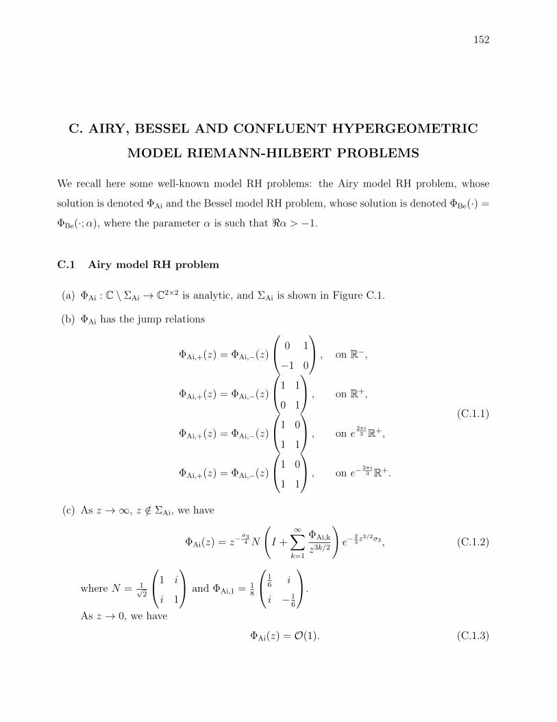
152

C. AIRY, BESSEL AND CONFLUENT HYPERGEOMETRIC

MODEL RIEMANN-HILBERT PROBLEMS

We recall here some well-known model RH problems: the Airy model RH problem, whose

solution is denoted ΦAi and the Bessel model RH problem, whose solution is denoted ΦBe(·) =

ΦBe(·;α), where the parameter α is such that <α > −1.

C.1 Airy model RH problem

(a) ΦAi : C \ ΣAi → C2×2 is analytic, and ΣAi is shown in Figure C.1.

(b) ΦAi has the jump relations

ΦAi,+(z) = ΦAi,−(z)

0 1

−1 0

, on R−,

ΦAi,+(z) = ΦAi,−(z)

1 1

0 1

, on R+,

ΦAi,+(z) = ΦAi,−(z)

1 0

1 1

, on e2πi3 R+,

ΦAi,+(z) = ΦAi,−(z)

1 0

1 1

, on e−2πi3 R+.

(C.1.1)

(c) As z →∞, z /∈ ΣAi, we have

ΦAi(z) = z−σ34 N

(I +

∞∑k=1

ΦAi,k

z3k/2

)e−

23z3/2σ3 , (C.1.2)

where N = 1√2

1 i

i 1

and ΦAi,1 = 18

16

i

i −16

.

As z → 0, we have

ΦAi(z) = O(1). (C.1.3)

153

2π3

0

Figure C.1. The jump contour ΣAi for ΦAi.

The Airy model RH problem was introduced and solved in [34]. We have

ΦAi(z) := MA ×

Ai(z) Ai(ω2z)

Ai′(z) ω2Ai′(ω2z)

e−πi6σ3 , for 0 < arg z < 2π

3,Ai(z) Ai(ω2z)

Ai′(z) ω2Ai′(ω2z)

e−πi6σ3

1 0

−1 1

, for 2π3< arg z < π,Ai(z) −ω2Ai(ωz)

Ai′(z) −Ai′(ωz)

e−πi6σ3

1 0

1 1

, for − π < arg z < −2π3,Ai(z) −ω2Ai(ωz)

Ai′(z) −Ai′(ωz)

e−πi6σ3 , for − 2π

3< arg z < 0,

(C.1.4)

with ω = e2πi3 , Ai the Airy function and

MA =√

2πeπi6

1 0

0 −i

. (C.1.5)

C.2 Bessel model RH problem

(a) ΦBe : C \ ΣBe → C2×2 is analytic, where ΣBe is shown in Figure C.2.

154

(b) ΦBe satisfies the jump conditions

ΦBe,+(z) = ΦBe,−(z)

0 1

−1 0

, z ∈ R−,

ΦBe,+(z) = ΦBe,−(z)

1 0

eπiα 1

, z ∈ e 2πi3 R+,

ΦBe,+(z) = ΦBe,−(z)

1 0

e−πiα 1

, z ∈ e− 2πi3 R+.

(C.2.1)

(c) As z →∞, z /∈ ΣBe, we have

ΦBe(z) = (2πz12 )−

σ32 N

(I +

∞∑k=1

ΦBe,kz−k/2

)e2z

12 σ3 , (C.2.2)

where ΦBe,1 = 116

−(1 + 4α2) −2i

−2i 1 + 4α2

.

(d) As z tends to 0, the behaviour of ΦBe(z) is

ΦBe(z) =

O(1) O(log z)

O(1) O(log z)

, | arg z| < 2π3,O(log z) O(log z)

O(log z) O(log z)

, 2π3< | arg z| < π,

, if <α = 0,

ΦBe(z) =

O(1) O(1)

O(1) O(1)

zα2σ3 , | arg z| < 2π

3,O(z−

α2 ) O(z−

α2 )

O(z−α2 ) O(z−

α2 )

, 2π3< | arg z| < π,

, if <α > 0,

ΦBe(z) =

O(zα2 ) O(z

α2 )

O(zα2 ) O(z

α2 )

, if <α < 0.

(C.2.3)

155

0

Figure C.2. The jump contour ΣBe for ΦBe(ζ).

This RH problem was introduced and solved in [10]. Its unique solution is given by

ΦBe(z) =

Iα(2z12 ) i

πKα(2z

12 )

2πiz12 I ′α(2z

12 ) −2z

12K ′α(2z

12 )

, | arg z| < 2π3,

12H

(1)α (2(−z)

12 ) 1

2H

(2)α (2(−z)

12 )

πz12

(H

(1)α

)′(2(−z)

12 ) πz

12

(H

(2)α

)′(2(−z)

12 )

eπiα2σ3 , 2π

3< arg z < π,

12H

(2)α (2(−z)

12 ) −1

2H

(1)α (2(−z)

12 )

−πz 12

(H

(2)α

)′(2(−z)

12 ) πz

12

(H

(1)α

)′(2(−z)

12 )

e−πiα2σ3 , −π < arg z < −2π

3,

(C.2.4)

where H(1)α and H

(2)α are the Hankel functions of the first and second kind, and Iα and Kα are

the modified Bessel functions of the first and second kind.

C.3 Confluent hypergeometric model RH problem

(a) ΦHG : C \ ΣHG → C2×2 is analytic, and ΣHG is shown in Figure C.3.

(b) ΦHG has the jump relations

ΦHG,+(z) = ΦHG,−(z)Jk, z ∈ Γk, (C.3.1)

156

V III

V II

V

V I

I

II

IV

III

Γ1Γ2

Γ5Γ4

Γ8

Γ3

Γ6

Γ70

π4

Figure C.3. The contour ΣHG = ∪8k=1Γk. Each Γk extends to ∞ and forms an

angle π4

with its adjacent ray.

where

J1 =

0 e−iπβ

−eiπβ 0

, J2 =

1 0

e−iπαeiπβ 1

, J3 = J7 =

e iπα2 0

0 e−iπα2

,

J4 =

1 0

eiπαe−iπβ 1

, J5 =

0 eiπβ

−e−iπβ 0

, J6 =

1 0

e−iπαe−iπβ 1

, J8 =

1 0

eiπαeiπβ 1

.

(c) As z →∞, z /∈ ΣHG, we have

ΦHG(z) =

(I +

∞∑k=1

ΦHG,k

zk

)z−βσ3e−

z2σ3M−1(z), (C.3.2)

where

ΦHG,1 = (β2 − α2

4)

−1 τ(α, β)

−τ(α,−β) 1

, τ(α, β) =−Γ(α

2− β)

Γ(α2

+ β + 1), (C.3.3)

157

and

M(z) =

eiπα4σ3e−iπβσ3 , π

2< arg z < π,

e−iπα4σ3e−iπβσ3 , π < arg z < 3π

2,

eiπα4σ3

0 1

−1 0

, −π2< arg z < 0,

e−iπα4σ3

0 1

−1 0

, 0 < arg z < π2.

(C.3.4)

The factor z−β in (C.3.2), has a cut along iR−, such that z−β ∈ R when z ∈ R+. As

z → 0, we have

ΦHG(z) =

O(1) O(log z)

O(1) O(log z)

, z ∈ II ∪ III ∪ V I ∪ V II,

O(log z) O(log z)

O(log z) O(log z)

, z ∈ I ∪ IV ∪ V ∪ V III,

, if <α = 0,

ΦHG(z) =

O(z<α2 ) O(z−

<α2 )

O(z<α2 ) O(z−

<α2 )

, z ∈ II ∪ III ∪ V I ∪ V II,

O(z−<α2 ) O(z−

<α2 )

O(z−<α2 ) O(z−

<α2 )

, z ∈ I ∪ IV ∪ V ∪ V III,

, if <α > 0,

ΦHG(z) =

O(z<α2 ) O(z

<α2 )

O(z<α2 ) O(z

<α2 )

, if <α < 0.

(C.3.5)

This model problem was introduced and solved in [5] for α = 0 and was later solved in the

general case in [9] and [33]. We consider the function

ΨHG(z;α, β) :=

Γ(1+α2−β)

Γ(1+α)G(α

2+ β, α; z)e−

πiα2 −Γ(1+α

2−β)

Γ(α2

+β)H(1 + α

2− β, α; ze−πi)

Γ(1+α2

+β)

Γ(1+α)G(1 + α

2+ β, α; z)e−

πiα2 H(α

2− β, α; ze−πi)

e−πiα4σ3 ,

(C.3.6)

158

where G and H are related to Whittaker functions :

G(a, α; z) =Mκ,µ(z)√

z, H(a, α; z) =

Wκ,µ(z)√z

, µ =α

2, κ =

1

2+α

2− a. (C.3.7)

Now, the solution to the confluent hypergeometric model Riemann-Hilbert problem is given

by

ΦHG(z) =

ΨHGJ−12 , z ∈ I,

ΨHG, z ∈ II,

ΨHGJ3, z ∈ III,

ΨHGJ3J−14 , z ∈ IV,

ΨHGJ−12 J−1

1 J−18 J−1

7 J6, z ∈ V,

ΨHGJ−12 J−1

1 J−18 J−1

7 , z ∈ V I,

ΨHGJ−12 J−1

1 J−18 , z ∈ V II,

ΨHGJ−12 J−1

1 , z ∈ V III,

(C.3.8)

where ΨHG(z) ≡ ΨHG(z;α, β).

159

VITA

Roozbeh Gharakhloo was born on June 9th, 1989 in Shiraz, Iran. He pursued professional

chess during middle school, high school and college years when he received gold medals in sev-

eral state and national tournaments. He studied Mechanical Engineering (Solid Mechanics)

in his undergraduate studies at Shiraz University, Iran. Towards the end of his undergraduate

studies, he found a deeper passion for mathematics which lead him to apply to the depart-

ment of Mathematical Sciences at IUPUI. His first intention was to do research in dynamical

systems, but he later changed his mind and considered working in the area of mathematical

physics. His mathematical research, Under guidance of professor Alexander Its, has been fo-

cused on the asymptotic analysis of structured determinants arising in random matrix theory,

statistical mechanics, theory of integrable operators and theory of orthogonal polynomials,

where he primarily employs the Riemann-Hilbert techniques.