Embed Size (px)
Citation preview

WORKING PAPERS
Asymmetric Pass-Through
in U.S. Gasoline Prices
Matthew Chesnes
WORKING PAPER NO. 302
June 2010___________________________________________________________________________
FTC Bureau of Economics working papers are preliminary materials circulated to stimulate discussionand critical comment. The analyses and conclusions set forth are those of the authors and do notnecessarily reflect the views of other members of the Bureau of Economics, other Commission staff, orthe Commission itself. Upon request, single copies of the paper will be provided. References inpublications to FTC Bureau of Economics working papers by FTC economists (other thanacknowledgment by a writer that he has access to such unpublished materials) should be cleared with theauthor to protect the tentative character of these papers.______________________________________________________________________________
BUREAU OF ECONOMICSFEDERAL TRADE COMMISSION
WASHINGTON, DC 20580

Asymmetric Pass-Through in U.S.Gasoline Prices∗
Matthew Chesnes†
Bureau of Economics
Federal Trade Commission
June 18, 2010
∗The opinions expressed here are those of the author and not necessarily those of the Federal TradeCommission or any of its Commissioners. I thank Michael Noel, Matthew Lewis, Chris Taylor, LouisSilvia, David Meyer, Doug Herman, and participants at the 2010 International Industrial Organiza-tion Conference for their suggestions and comments. Elisabeth Murphy provided excellent researchassistance. All remaining errors are my own.
†Email: [email protected].
1

Abstract
This paper presents new evidence of asymmetric pass-through, the notion thatupward cost shocks are passed through faster than downward cost shocks, in U.S.gasoline prices. Much of the extant literature comes to seemingly contradictoryconclusions about the existence of an asymmetry, though the differences may bedue to different aggregation (both over time and geographic markets) and the useof different price series including crude oil, wholesale, and retail gasoline prices. Iutilize a large and detailed dataset to determine where evidence of a pass-throughasymmetry exists, and how it depends on the aggregation and price series chosenby the researcher.
Using the standard error correction model, I find evidence of pass-throughasymmetry in the response of daily and weekly retail prices to wholesale rack pricechanges, though the magnitude varies by geographic market. On average, retailprices rise more than four times as fast as they fall. Branded gasoline featuressignificantly more asymmetry with respect to rack prices compared with unbrandedgasoline. Over time, nation-wide asymmetry varies significantly from year to yearpeaking in 2005. Midwest cities, like Louisville and Minneapolis, feature moreasymmetry compared with other parts of the country. F-tests broadly confirmthe results and illustrate that data selection and aggregation, as well as modelspecification, can have important implications on the findings of asymmetric pass-through.
2

1 Introduction
There is a large literature analyzing the cost to price pass-through in industries ranging
from automobiles (Gron and Swenson (1982)), to cheese products (Kim and Cotterill
(2008)), to the beef industry (Goodwin and Holt (1999)). The literature has not only
focused on the ability of firms to successfully capture rents when input costs change,
but also on how the rate of pass-through varies when the costs increase versus decrease.
In the gasoline industry, this asymmetric phenomenon is known as rockets and feathers,
reflecting the fact that retail prices tend to increase quickly when costs (say, wholesale
gasoline prices) rise, but drift down slowly when they fall.1 Much of the extant literature
comes to seemingly contradictory conclusions about the existence of this phenomenon,
though the differences may be due to different data sources, price series, aggregation
over time and across geographic areas, as well as misspecified models. In this paper,
I re-examine the pass-through in gasoline prices using a detailed dataset available at a
high frequency, across many cities, and at several price levels in the vertical distribution
process for gasoline.
The gasoline industry has been the focus of a particularly large amount of research
on pass-through for several reasons. Gasoline is a fairly homogeneous product and both
retail and intermediate wholesale prices are relatively transparent compared with other
industries.2 Much of the variation in gasoline prices is driven by the price of crude
oil, the key input into gasoline.3 This crude oil is traded on a world market and the
price is also transparent to market players and to consumers. In spite of this, there are
1The production and distribution of gasoline is just one part of the petroleum industry, which pro-duces a whole range of refined products. The rockets and feathers literature has focused primarily ongasoline prices.
2Rack prices for wholesale gasoline are observable and in 2009, refiner rack sales accounted for 60% ofthe total gasoline supplied in the US. See http://tonto.eia.doe.gov/dnav/pet/pet_cons_refmg_c_nus_epm0_mgalpd_a.htm and http://tonto.eia.doe.gov/dnav/pet/pet_cons_psup_dc_nus_mbbl_m.htm. The rest is sold to lessee-dealer stations at (unobserved) dealer-tank-wagon (DTW) prices andvia transfer prices to refiner-operated stations.
3See The Federal Trade Commission, “Gasoline Price Changes: The Dynamics of Supply, Demandand Competition,” 2005.
3

dynamics present in the gasoline industry which are difficult to explain with competitive
or oligopolistic economic models.
The literature on rockets and feathers dates back to at least 1991 when Robert
Bacon found evidence of an asymmetric response in gasoline prices in the UK. Since that
time, others have found evidence of the phenomenon including Borenstein, Cameron,
and Gilbert (1997, hereafter BCG), Lewis (forthcoming), Ye et. al. (2005), and most
recently, Deltas (2008). These studies all utilize some form of an error correction model
(outlined below) and consider some combination of crude oil prices, wholesale prices (rack
or spot), and retail gasoline prices. They also vary by the geography they consider and
how the data are aggregated over time (i.e., daily, weekly, or monthly). There are also
several papers that, due to either a different data source or model, find no evidence of an
asymmetric price response including Bachmeier and Griffin (2003) and Godby (2000).
The former paper also tests BCG results using daily data; however they only focus on
the transmission of crude oil to spot gasoline prices.
This paper is similar to BCG in that I analyze several different prices (crude oil, spot
gasoline, rack, and retail prices) over a long period of time. However, unlike BCG who
use weekly and bi-weekly data from the Lundberg Survey, I have access to daily data
on all prices. I also avoid a modeling assumption by BCG (discussed below) which was
questioned by Bachmeier and Griffin (2003) and instead use a more standard approach.
If it exists, there is little consensus on what causes the asymmetric response, though
explanations range from consumer search costs, to explicit or implicit collusion, to in-
ventory management by consumers. Deltas, for example, looks at how the asymmetric
response varies with the level of retail market power and finds more asymmetry in mar-
kets with relatively more retail market power.4 Lewis (forthcoming) and others posit
4Market power is proxied by the average markup observed in the market over his sample period. It istempting to assume that markets in which firms face less competition will feature firms quickly passingon cost increases to consumers, and only slowly (or possibly never) passing on cost savings. Marketswith many competing firms should feature perfect pass-through. For industry-wide cost changes, this isgenerally true, however the opposite results when the cost change is firm-specific. Bulow and Pfleiderer(1983) show that firm-specific cost changes are more completely passed through the less competitive is
4

that consumer search behavior could be causing the asymmetric response. If consumers
are more likely to search for a low price when prices are expected to rise, then competi-
tion will be fierce when costs are rising and margins tight. However, if prices are falling,
consumers may search less and this provides retailers with short-term market power and
allows them to slowly lower prices and increase their margins. If this is the case, it
still does not explain why asymmetric adjustment varies across time or across different
geographic areas.
Asymmetric adjustment of downstream prices to changes in an upstream cost (such
as a wholesale price) is generally divided into two forms: amount asymmetry and pattern
asymmetry. Amount asymmetry occurs when the aggregate change over a period of time
is different when costs are rising versus when they are falling. This asymmetry is not the
focus of most studies because it would imply that the upstream and downstream prices
would diverge over time, which is not the case with gasoline prices. Pattern asymmetry
involves differences in the relative speed of pass-through. As an example, one may find
evidence of pattern asymmetry if a 10% increase in wholesale prices leads to a 10%
increase in retail prices after one week, but an equivalent decrease in wholesale prices
leads to only a 5% decline in retail prices after one week. Consistent with the literature,
I will focus my analysis on pattern asymmetry.
In this study, I look for pattern asymmetry in pass-through, and I vary the geography,
the time aggregation, and products considered. I find the strongest evidence of pattern
asymmetry in the rack to retail prices at both the city and national level. On average,
retail prices rise more than four times as fast as they fall. Branded gasoline features
significantly more asymmetry compared with unbranded gasoline.
Asymmetry varies significantly from year to year and across cities. For example,
while in Los Angeles, the asymmetry of branded rack to retail price changes is fairly
the market. (See also, Ten Kate and Niels (2005).) The reason is that when faced with a cost decrease,say, firms with a greater market share will benefit relatively more from the increase in quantity demandedwhich more than offsets the lower revenue from passing on the cost decrease in the form of lower prices.
5

constant over time, in Phoenix, it is over four times as high in 2005 versus in 2007.
Using weekly instead of daily data, tends to attenuate the evidence of asymmetry in
some cases, though increases it in others.
The paper proceeds as follows. In section 2, I outline the model that I employ and
specification tests that need to be run to justify its use. I discuss the data and provide
basic descriptive statistics in section 3 and present the results of my model in section
4, including asymmetric pass-through results for different geographic areas, at different
levels of time aggregation, and for different products. In section 5, I conclude and provide
a brief outline of a complementary paper which seeks to explain why pass-through rates
and asymmetry vary by city and over time.
2 Model
I estimate an error correction model (ECM) frequently used in the literature, though in
various forms (e.g., Bachmeier and Griffin (2003)). I estimate two versions of the model:
one which is run individually for each city (metro area)5 and the other is a national-level
model with fixed effects included for each city, which allows for different markups in
each city.6 The latter regression measures the average pass-through rate across all cities,
while allowing the long-term relationship to vary by city. I allow for a difference in the
pass-through of positive and negative upstream price changes.
While I estimate the model for several pairs of upstream and downstream prices, for
simplicity, the following is the rack to retail pass-through model for a given city:
5Most of the metro areas in my sample are major cities. Some cities near state borders are splitacross state lines, so for example, Louisville, KY and Louisville, IN are separate metro areas. See figureA.1 for an example. This is important because often different types of gasoline (e.g., conventional, RFG,and California Air Resources Board (CARB) gasoline) are sold in different states.
6I use the term “national-level,” though prices are not aggregated, but instead the specificationincludes prices from all major cities in my dataset.
6

∆Retailt =
L+1∑
i=0
β+1i∆
+Rackt−i +
L−1∑i=0
β−1i∆
−Rackt−i (1)
+
L+2∑
i=1
β+2i∆
+Retailt−i +
L−2∑i=1
β−2i∆
−Retailt−i
+ β+3 (Retailt−1 − γ0 − γ1Rackt−1)︸ ︷︷ ︸
z+t−1
+ β−3 (Retailt−1 − γ0 − γ1Rackt−1)︸ ︷︷ ︸
z−t−1
+εt.
Note ∆Retailt−i = Retailt−i −Retailt−(i−1). Lag lengths are determined by minimiz-
ing the Bayesian Information Criterion (BIC):
BIC = K ∗ log(N) + N ∗ [Log(RSS/N)], (2)
where K is the number of parameters to be estimated, N is the number of observations,
and RSS = ε̂′ε̂ from equation 1. I could allow the lag lengths to vary separately for
positive and negative changes as well as for rack and retail prices. However, since deter-
mining the optimal lag lengths for each price series, versus using a fixed (and equal) lag
length for all, does not affect the qualitative results, in the analysis below I fix the lag
length at 21 days in all regressions. This also allows me to compare regressions across
cities and over time since I will utilize the same specification in each.
The expression zt−1 = Retailt−1 − γ0 − γ1Rackt−1 is the error correction term, and
it captures the long-run relationship between the upstream and downstream prices. β+3
and β−3 should both be negative: if retail prices are above their equilibrium level (zt−1 >
0), retail prices should fall and if they are below the level predicted by the rack price
(zt−1 < 0), retail prices should rise.
Following the two-step method proposed by Engle and Granger (1987), I estimate γ0
7

and γ1 by running OLS on the following equation:
Retailt−1 = γ0 + γ1Rackt−1 + zt−1. (3)
The residuals, zt−1, are then inserted directly into the model.7 BGC estimate the long-
term relationship in the same step as the rest of the parameters and instrument for
the upstream prices to control for possible endogeneity. As outlined in Bachmeier and
Griffin (2003), this may lead to problems with the resulting estimates.8 Once I obtain
the residuals, I can estimate equation 1 by OLS.
The national-level regression is similar, though it includes city-level fixed effects in
the error correction term:
Retailt−1 = γ0 + γ1Rackt−1 +27∑i=2
φiCityi + zt−1. (4)
As mentioned in the introduction, there are two potential types of asymmetry:
amount and pattern. In terms of the model parameters, amount asymmetry would
be of the form:
L+1∑
i=0
β+1i 6=
L−1∑i=0
β−1i, (5)
however, this cannot exist over the long-term since upstream and downstream prices do
not tend to drift apart. Pattern asymmetry could be found if any one of the following
7Since the two series are cointegrated, the OLS regression yields super-consistent estimates of the γparameters. The estimates can then be inserted into the model as if they were known parameters.
8BCG run a two-stage least squares regression and instrument for the upstream price with the crudeoil price in England and a forward prices of crude in the US. However, while they reject the null thatthere is no endogeneity in the prices, their 2SLS and OLS estimates are very similar.
8

three conditions are met:
β+1i 6= β−
1i for some i (6)
|β+3 | 6= |β−
3 | (7)
L+1 6= L−
1 or L+2 6= L−
2 . (8)
The asymmetry in equation 6 is the one commonly analyzed in the literature. While
the aggregate pass-through should be the same for positive and negative rack price
changes, the pattern of the pass-through may be different. If any of the coefficients on
the same lag are different, this is evidence of pattern asymmetry. The coefficients on the
first lag, β+1,1 and β−
1,1 are particularly important because they measure the contempora-
neous speed of pass-through, assuming the model could be approximated as a first-order
difference equation.
The second pattern asymmetry (noting again that β3 should be negative reflecting
mean-reversion) involves the speed at which relative prices return to their long-term
equilibrium levels. We have evidence of the rockets and feathers type of asymmetry if
this mean reversion is slower (closer to zero) when retail prices are above their long-term
levels and faster (closer to one) when retail prices should be adjusting upwards toward
their long-term levels.
Finally, if I allowed the BIC-optimum lag lengths to vary for positive and negative
changes, further evidence of pattern asymmetry is obtained if the optimal lag lengths
are different. Though this is often the case, I fix the lag lengths and focus most of my
attention on asymmetries in contemporaneous pass-through and mean reversion via the
error correction term.
9

3 Data and Descriptive Statistics
I combine two datasets to perform the analysis. Spot prices are available from Reuters
via the Energy Information Administration (EIA) and rack and retail price data are
from the Oil Price Information Service (OPIS). All data are available daily (I will dis-
cuss weekends and missing values below) from January 1999 through December 2009.
Summary statistics are provided in tables 1, 2, and 3. All prices are reported in cents
per gallon (cpg).
Spot prices include the price of West Texas Intermediate (WTI) crude oil at Cushing,
Oklahoma. I also obtain the conventional regular and reformulated regular gasoline prices
along with the RBOB9 spot for New York harbor, the Gulf Coast, and Los Angeles. Spot
prices are reported as of the close of day, Monday through Friday.
Average MarginSpot Price N Min Mean Max Std Dev Date Range Over WTIConventional - NY 2,726 29.03 131.33 341.55 66.86 Jan 1999 - Dec 2009 16.93Conventional - Gulf 2,726 27.00 130.69 487.25 68.43 Jan 1999 - Dec 2009 16.29Conventional - LA 2,726 38.00 143.91 382.51 69.69 Jan 1999 - Dec 2009 29.51RFG - NY 1,859 30.43 101.61 282.95 41.19 Jan 1999 - June 2006 18.24RFG - Gulf 1,834 28.65 99.87 344.50 41.52 Jan 1999 - May 2006 17.66RFG - LA 1,222 40.00 91.04 167.00 22.09 Jan 1999 - Nov 2003 28.04RBOB - NY 1,340 75.33 188.64 357.60 56.37 July 2004 - Dec 2009 23.90RBOB - Gulf 889 82.30 207.06 487.25 63.87 May 2006 - Dec 2009 26.09RBOB - LA 1,679 78.00 188.54 389.60 62.30 Mar 2003 - Dec 2009 41.21WTI 2,726 27.10 114.41 345.98 62.71 Jan 1999 - Dec 2009 -
Table 1: Daily Spot Prices (Cents per Gallon)
I use rack prices from OPIS for 20 U.S. cities. These rack prices are for the type of
gasoline used in each city since many cities utilize different types of gasoline (conven-
tional, RFG, etc.). In some cases, rack prices for different types of gasoline are reported
in the same city. In these cases, I use the rack price that corresponds to the type of
gasoline that is used in each retail market area. For example, the Fairfax, VA rack
reports both conventional and RFG prices. Since I observe retail data for stations in
9Reformulated Blendstock for Oxygenate Blending.
10

Washington, DC, as well as the Virginia, Maryland, and West Virginia suburbs of DC,
I match the RFG rack price to DC, VA, and MD since each uses primarily RFG, while
the WV retail prices are matched to the conventional rack since that area primarily uses
conventional gasoline. Rack prices are reported as of 9AM, Monday through Saturday,
and are available for both branded and unbranded products.
Border Average MarginStates N Min Mean Max Std Dev Date Range Over WTI
Atlanta (Conventional) 4,014 33.09 126.90 354.29 72.11 Jan 1997 - Dec 2009 25.17Boston (RFG) 4,065 36.05 131.09 362.22 70.51 Jan 1997 - Dec 2009 29.05Chicago (RFG) 4,066 38.94 135.05 363.34 70.77 Jan 1997 - Dec 2009 33.21Cleveland (Conventional) 4,066 32.33 128.70 359.30 70.68 Jan 1997 - Dec 2009 26.97Dallas (RFG) 4,066 34.65 129.35 356.63 71.14 Jan 1997 - Dec 2009 27.73Denver (Conventional) 4,066 33.37 129.55 364.76 70.82 Jan 1997 - Dec 2009 27.64Detroit (Conventional) 4,066 31.10 128.73 361.20 71.17 Jan 1997 - Dec 2009 27.04Fairfax (Conventional) WV 4,066 34.46 125.95 351.70 70.12 Jan 1997 - Dec 2009 23.76Fairfax (RFG) DC, MD, VA 4,066 37.11 130.35 356.28 71.52 Jan 1997 - Dec 2009 28.49Houston (RFG) 4,065 33.77 127.19 355.03 70.71 Jan 1997 - Dec 2009 25.37Los Angeles (CARB) 2,825 59.28 174.35 392.91 66.58 Dec 2000 - Dec 2009 47.56Louisville (Conventional) IN 4,049 32.66 128.32 355.70 70.66 Jan 1997 - Dec 2009 26.29Louisville (RFG) KY 2,857 39.65 160.73 376.64 77.56 Feb 1998 - Dec 2009 40.54Miami (Conventional) 4,066 34.84 126.63 353.51 70.97 Jan 1997 - Dec 2009 24.64Minneapolis (Conventional) 4,064 35.18 130.67 357.47 70.81 Jan 1997 - Dec 2009 28.90New Orleans (Conventional) 4,066 32.81 124.01 350.88 69.96 Jan 1997 - Dec 2009 21.86Newark (RFG) 3,803 38.82 134.25 355.16 69.20 Mar 1997 - Dec 2009 27.17Phoenix (Conventional) 4,066 43.60 140.32 366.58 71.25 Jan 1997 - Dec 2009 39.44Salt Lake City (Conventional) 4,065 37.05 134.35 367.52 69.56 Jan 1997 - Dec 2009 32.22San Francisco (CARB) 2,809 59.23 171.41 375.37 65.27 Jan 2001 - Dec 2009 44.24Seattle (Conventional) 4,066 41.66 135.62 364.57 70.37 Jan 1997 - Dec 2009 34.19St Louis (Conventional) IL 4,065 31.94 128.38 355.41 71.62 Jan 1997 - Dec 2009 26.62St Louis (RFG) MO 3,337 57.92 149.81 359.20 66.52 May 1999 - Dec 2009 32.47Racks that service multiple states with different types of wholesale gasoline are indicated in the "Boarder States" column. For example, the Fairfax, VA rack sells RFG to stations in Washington DC and its nearby suburbs, while it sells conventional gasoline to stations in West Virginia.
Table 2: Daily Rack Prices (Cents per Gallon)
Finally, I utilize pre-tax retail price data from OPIS for the 27 retail metro areas all
within the 20 cities for which I have rack prices. Retail prices are (usually) end of the
day prices as they are recorded from the last swipe of a consumer’s “fleet-card” on a
given day.10 OPIS averages all the prices they receive each day (at most one from each
station) to determine the price for the metro area. After 2001, the prices are reported
every day of the week. OPIS samples over 100,000 stations each day and covers branded
and unbranded stations. The three most expensive cities for retail gasoline in 2008 were
10See http://www.opisretail.com/methodology.html for more information on OPIS’s retail data. Morethan one-half of the stations in the OPIS sample report a price each day, though the sample of stationsmay change from day to day.
11

Miami, San Francisco, and Washington DC. These three cities also featured the highest
retail markups over the wholesale price.
Average MarginN Min Mean Max Std Dev Date Range Over Rack
Atlanta 3,817 49.35 152.19 346.67 69.64 Jan 1999 - Dec 2009 9.35Boston 3,817 58.16 163.20 366.50 68.77 Jan 1999 - Dec 2009 16.58Chicago 3,817 55.82 163.88 365.56 70.41 Jan 1999 - Dec 2009 13.25Cleveland 3,817 45.37 156.72 358.05 68.93 Jan 1999 - Dec 2009 12.30Dallas 3,817 50.31 156.40 359.55 70.41 Jan 1999 - Dec 2009 11.14Denver 3,816 49.03 158.37 360.39 70.36 Jan 1999 - Dec 2009 13.39Detroit 3,817 46.10 155.22 360.01 69.34 Jan 1999 - Dec 2009 10.71Houston 3,817 51.19 154.57 357.81 70.11 Jan 1999 - Dec 2009 11.64Los Angeles 3,816 56.39 175.32 392.76 71.13 Jan 1999 - Dec 2009 13.46Louisville IN 3,815 42.28 153.94 364.86 69.26 Jan 1999 - Dec 2009 10.20Louisville KY 3,816 47.53 163.66 389.74 72.31 Jan 1999 - Dec 2009 7.51Miami 3,817 68.21 177.18 383.47 73.14 Jan 1999 - Dec 2009 34.61Minneapolis MN 3,817 54.06 158.88 360.77 68.43 Jan 1999 - Dec 2009 12.58Minneapolis WI 3,815 51.50 158.18 353.03 68.37 Jan 1999 - Dec 2009 11.78New Orleans 3,815 56.13 157.52 362.36 70.84 Jan 1999 - Dec 2009 18.00Newark 3,816 57.82 163.97 367.73 69.48 Jan 1999 - Dec 2009 19.41New York City 3,817 60.55 166.93 365.48 68.54 Jan 1999 - Dec 2009 22.32Pheonix 3,816 54.55 167.61 376.72 69.38 Jan 1999 - Dec 2009 10.50Salt Lake City 3,816 46.67 158.08 373.46 70.96 Jan 1999 - Dec 2009 8.48San Francisco 3,815 80.72 188.67 390.37 67.09 Jan 1999 - Dec 2009 28.24Seattle 3,816 63.10 171.78 384.57 69.82 Jan 1999 - Dec 2009 20.03St Louis IL 3,817 43.00 150.40 351.03 68.03 Jan 1999 - Dec 2009 6.27St Louis MO 3,816 42.16 155.76 362.64 70.02 Jan 1999 - Dec 2009 6.56Washington DC 3,756 58.14 174.30 380.73 73.39 Jan 1999 - Dec 2009 26.97Washington MD 3,817 54.27 165.07 368.13 71.50 Jan 1999 - Dec 2009 18.97Washington VA 3,817 50.87 160.03 363.64 70.84 Jan 1999 - Dec 2009 13.97Washington WV 3,815 43.27 156.50 360.02 71.32 Jan 1999 - Dec 2009 14.95This table shows statistics by "retail market area" as reported by OPIS. Prices are generated using Fleet Card purchases from all stations in the area.
Table 3: Daily Retail Prices (Cents per Gallon)
Given the different reporting times of day for each price series, when running re-
gressions using daily data, it is important that lags are used where appropriate. For
example, when considering the speed of pass-through from rack to retail, I can consider
the effect for the same time stamp since end of day retail prices have a chance to adjust
to a change in the rack price observed at the beginning of the day. However, in the
spot to rack pass-through regressions, I use the lagged spot price because these two price
series are reported at the same time of day.
12

Border ProportionStates N Mean N Mean Unbranded > Branded
Atlanta (Conventional) 4,014 126.90 4,002 123.81 0.049Boston (RFG) 4,065 131.09 4,066 126.20 0.039Chicago (RFG) 4,066 135.05 4,066 131.75 0.042Cleveland (Conventional) 4,066 128.70 4,062 125.90 0.072Dallas (RFG) 4,066 129.35 4,066 126.67 0.083Denver (Conventional) 4,066 129.55 4,066 127.07 0.066Detroit (Conventional) 4,066 128.73 4,016 125.44 0.069Fairfax (Conventional) WV 4,066 125.95 4,004 123.60 0.065Fairfax (RFG) DC, MD, VA 4,066 130.35 4,066 126.69 0.050Houston (RFG) 4,065 127.19 4,065 124.38 0.071Los Angeles (CARB) 2,825 174.35 2,582 176.58 0.282Louisville (Conventional) IN 4,049 128.32 4,062 124.78 0.051Louisville (RFG) KY 2,857 160.73 3,723 144.23 0.128Miami (Conventional) 4,066 126.63 4,066 123.64 0.041Minneapolis (Conventional) 4,064 130.67 4,066 127.65 0.039New Orleans (Conventional) 4,066 124.01 4,066 120.77 0.035Newark (RFG) 3,803 134.25 3,809 129.57 0.052Phoenix (Conventional) 4,066 140.32 4,066 134.14 0.142Salt Lake City (Conventional) 4,065 134.35 4,065 131.96 0.090San Francisco (CARB) 2,809 171.41 2,412 178.16 0.287Seattle (Conventional) 4,066 135.62 4,066 130.89 0.164St Louis (Conventional) IL 4,065 128.38 4,025 124.99 0.066St Louis (RFG) MO 3,337 149.81 3,323 150.13 0.270
Branded Unbranded
Table 4: Branded versus Unbranded Rack Prices (Cents per Gallon)
In table 4, I report statistics on branded versus unbranded rack prices. Generally,
unbranded gasoline is more homogeneous across refiners because it includes only a generic
package of additives and lacks a brand name premium. Therefore, in most cases, branded
gasoline is about 5 cents more expensive than unbranded. However, as evidence in the
right-hand column shows, at times the unbranded price actually exceeds the branded
price and this happens quite often in Los Angeles, San Francisco, and St. Louis. Many
of these inversions follow supply shocks (e.g., hurricanes and refinery outages) as refiners
may be giving priority to their branded customers to maintain the brand image, resulting
in a more severe supply reduction for unbranded gasoline. Whatever the cause, below I
investigate the asymmetric response for branded and unbranded fuel separately.
13

3.1 Data Issues
Before focusing on the results, there are a few issues with the data that need to be
addressed. I run my regressions at both a daily and a weekly frequency. Weekly data
was generated as the simple average of the daily series. This means that sometimes the
average is over five days, other times six days, four days, etc. Early in the sample, the
data suffer from many missing values, though starting in 2002, the data are much more
complete. Therefore, I restrict the regressions to dates from January 2002 - December
2009.
Due to holidays, etc, there are still some missing values in the daily data. Instead of
interpolating on each of these days, I do the following:
1. Include any day that has data on both the upstream and downstream price.
2. Do not include any date that is missing both the upstream and downstream price.
3. Include a partial observation if it occurs on Monday - Friday, leaving the missingvalue in the data.11
This means that the duration between observations is usually one day (adjacent days)
or three days (for weekends) though at times may be longer if both prices are missing for
a period of time. I have analyzed the distribution of changes in all the prices as it varies
by the number of days between adjacent non-missing observations. I find that there is
almost no “weekend effect” in that the changes in price from Friday to Monday have
the same distribution as the changes on adjacent days. However, there are a few longer
periods in the data with missing values and the distribution of changes is much wider.
Therefore, I control for these large jumps by including a dummy variable which equals
one if any of the changes on the upstream or downstream price are for a period of five
11The reason I include the partial observation instead of dropping it is to eliminate situations wheretwo lagged differences are included in an observation, one over adjacent days, and the other over a muchlonger number of days. In effect, this method results in dropping several observations when I estimatethe model, but reduces the number of long gaps between consequative observations.
14

days or more. With this set of observations, lags are formed and if missing values are
present in any observation, it is removed from the analysis.12
Finally, at one time the spot price for RFG was for reformulated gasoline blended
with MTBE, which has now been banned in most states.13 It has been replaced by the
RBOB spot price, which is RFG that will eventually get blended with an oxygenate
(typically ethanol). In New York and LA, there is some overlap in the two series so I
create my complete spot price for RFG as the old RFG spot for the early part of the
sample, and as soon as the RBOB spot is available, I switch to that price. The two
prices are similar to each other during the overlap period.14 For the Gulf Coast, there is
no overlap (the RFG spot ends on one day and the RBOB spot begins being reported
on the very next day) so I concatenate the two series to form my complete RFG spot
price. However, the RBOB price on its first day being reported is 38 cents higher than
the RFG spot on the previous day.15 I have done robustness checks by only running
the regression using dates where I observe the RFG spot price and the results are very
similar.
4 Results
Before analyzing the results, it is important to test for stationarity of the regressors. I
run Augmented Dickey Fuller (ADF) tests which show that all price series do indeed
have a unit root so first differencing is necessary. I then run another ADF test on each
set of price series together and confirm that the upstream and downstream price series
are cointegrated (i.e., the residuals from the long-run regression equations 3 and 4 are
12Removing observations only after lags are formed guarantees that the lagged differences in a givenobservation are all over approximately the same (small) duration of time.
13In others, the liability protection has been removed so refiners are reluctant to use it.14A simple regression of the RFG spot on the RBOB spot during the overlap yields a slope coefficient
of 0.94 for NY and 0.95 for LA.15Compared with mean absolute day to day changes for RFG and RBOB of 2.6 and 5.1 cents respec-
tively.
15

stationary).16 Therefore, estimating the long-term relationship in the first stage provides
super-consistent estimates which can be entered into the model directly. Durbin Watson
tests for autocorrelation correlation are also run and fail to reject the hypothesis that
there is no autocorrelation in the residuals for each model.
I divide the results into several sections which consider the differences in pattern
asymmetry among different price relationships, across cities and in the national regres-
sion, by the time aggregation of the data, for branded versus unbranded wholesale gaso-
line, and over time. Finally, I show formal F-tests of pattern asymmetry for each type
of model.
4.1 Price Relationships
I investigate pass-through asymmetry for combinations of the crude oil price, the gasoline
spot price, the branded and unbranded rack prices, and the retail price series. The
following tables and figures summarize the results of equation 4, which incorporate data
from all cities and includes city-level fixed effects in the long-term first-stage regression.
The relationships include the following:
1. Crude oil price to the gasoline spot price, the rack prices, and the retail price.17
2. Closest gasoline spot price to the rack prices and the retail price.18
3. Rack prices to the retail price.
Complete results for one of these regressions (rack to retail) is shown in table A.1
in the appendix. However, following the literature on asymmetric pass-through, it is
much easier to present the results graphically. The reason is that a one-time change
in the upstream price will have an immediate effect on the downstream price, but the
16ADF test statistics on the rack to retail price relationship are all greater than six compared with a5% critical value of 3.33 from MacKinnon (2010).
17I estimate the crude to spot relationship for each of the six spot prices available on EIA’s website:conventional gasoline and RFG in NY, Houston, and LA.
18I use the NY spot price for Boston and Newark. I use the LA spot price for LA, San Francisco,Phoenix, Salt Lake City and Seattle. For the rest, I use the Gulf Coast spot price.
16

total effect may be drawn out over a period of days and include both the short-term
speed of adjustment (the β1 terms in equation 1), the own-lag effects (the β2 terms), and
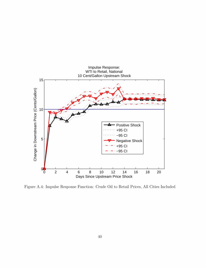
the long-term error correction effects (the β3 terms). For this reason, I present impulse
response functions which trace out the effects of a ten cent per gallon change (positive
or negative) in the upstream price on the downstream price over a period of several days
following the shock. The 95% confidence bands are also shown in each graph.19
Figures 1 and 2 below, along with figures A.2, A.3, A.4, and A.5 in the appendix
display the impulse response function tracing out the effect on the downstream price of
a 10 cpg change in the upstream price. While each of the figures shows some kind of
asymmetric response, the rockets and feathers type (where the response time of positive
shocks exceeds negative shocks) is strongest in the rack to retail and spot to retail
relationships. However, while the asymmetry in both of these relationships becomes
statistically insignificant after about seven to ten days, the asymmetry in spot to retail
prices is significantly smaller than rack to retail. A weaker (and sometimes reverse)
asymmetry is shown in the crude to gasoline spot, rack, and retail price regressions.
Bacon (1991) found a similar asymmetry in rack to retail prices, while Bachmeier and
Griffin (2003) find no evidence of asymmetry in the crude oil to gasoline spot price trans-
mission, consistent with my results. BCG (1997) do not find any significant asymmetry
in the spot to retail relationship, though their study relies on bi-weekly data.
4.2 Individual City Results
The evidence of asymmetries found in the previous section is mostly confirmed by re-
gressions run at the individual city level. In table 5, I present results on the difference in
the first coefficients on the upstream price for positive and negative changes. Though a
complete picture of pass-through asymmetry can only be seen from an impulse response
19To account for possible nonlinearities in the relationships between the upstream and downstreamprices, I consider an upstream price increase from 200 cpg to 210 cpg and a corresponding decrease from210 cpg to 200 cpg.
17

0 2 4 6 8 10 12 14 16 18 200
5
10
15
Days Since Upstream Price Shock
Cha
nge
in D
owns
trea
m P
rice
(Cen
ts/G
allo
n)
Impulse Response:Branded Rack to Retail, National10 Cent/Gallon Upstream Shock
Positive Shock+95 CI−95 CINegative Shock+95 CI−95 CI
Figure 1: Impulse Response Function: Rack to Retail Prices, All Cities Included
graph, this first coefficient embodies the speed of pass-through if we think of the model
as approximating a first-order difference equation.
I include the difference by city and for each of the city-specific price relationships. The
difference in the β1 coefficients in the crude oil to rack and retail price relationships are
mostly insignificant or have a reverse asymmetry as measured by the speed coefficient.
The spot to rack regressions reveal asymmetry in several cities, including Detroit, Miami,
and St. Louis. The final two columns on rack to retail prices again confirm the strong
asymmetry in all cities as was found in the previous section. The asymmetry is the
strongest in Cleveland, Detroit, Louisville, and Minneapolis, while it is weakest in San
Francisco and the West Virginia suburbs of Washington DC.
18
-,-' _.-' -... . .. ,.' .

0 2 4 6 8 10 12 14 16 18 200
5
10
15
Days Since Upstream Price Shock
Cha
nge
in D
owns
trea
m P
rice
(Cen
ts/G
allo
n)
Impulse Response:Spot to Retail, National
10 Cent/Gallon Upstream Shock
Positive Shock+95 CI−95 CINegative Shock+95 CI−95 CI
Figure 2: Impulse Response Function: Gasoline Spot to Retail Prices, All Cities Included
In table 6, I present the results on the form of asymmetry shown in equation 7: the
difference between the positive and negative coefficients on the error correction term.
The results for the rack to retail relationships are similar to above, and the long-term
correction asymmetry appears more in the crude to rack and retail price relationships,
while it has the opposite sign in spot to rack price regressions.
The type of fuel utilized in each city is also related to the degree of pass-through
asymmetry. For example, St. Louis IL, Louisville IN, and Washington WV all utilize
conventional gasoline and all have lower asymmetry than their neighboring retail metro
areas which utilize RFG.
While the differences in the speed of adjustment and error correction terms provides
19
----... ... : :,..:. ... .-,. ., . ':: ~ : ~ ', ,;.. ,,'; .. : : :": ,' ;":

Atlanta -0.20*** -0.09 -0.02 0.01 0.03 0.23*** 0.14***Boston -0.10*** -0.12* -0.05*** 0.03 0.12*** 0.14*** 0.07***Chicago -0.04 -0.04 -0.06** 0.06** -0.02 0.13*** 0.09***Cleveland -0.09* 0.10 -0.21*** 0.05* -0.06 0.31*** 0.21***Dallas -0.21*** -0.11* -0.05*** 0.03 0.02 0.12*** 0.07***Denver -0.09** -0.11** -0.02 0.02 0.03 0.11*** 0.08***Detroit -0.01 0.16** -0.09** 0.08*** 0.09** 0.32*** 0.20***Washington DC -0.14*** -0.05 -0.08*** -0.01 -0.10*** 0.15*** 0.08***Washington MD -0.14*** -0.05 -0.03 -0.01 -0.10*** 0.13*** 0.06***Washington VA -0.14*** -0.05 -0.03* -0.01 -0.10*** 0.12*** 0.08***Washington WV -0.14*** 0.06 -0.10*** 0.05*** -0.04 0.07*** 0.01Houston -0.14*** -0.02 -0.06*** 0.00 0.13*** 0.14*** 0.06***Los Angeles -0.03 -0.13 -0.01 0.02 0.07 0.16*** 0.01**Louisville IN -0.20*** -0.10 -0.15*** 0.00 -0.01 0.27*** 0.16***Louisville KY -0.19*** -0.08 -0.19** -0.04 -0.10*** 0.37*** 0.27***Miami -0.16*** -0.15** -0.07*** 0.04** 0.20*** 0.15*** 0.07***Minneapolis St Paul MN -0.08 -0.16** -0.17*** 0.07*** -0.17*** 0.38*** 0.31***Minneapolis St Paul WI -0.08 -0.16** -0.13*** 0.07*** -0.17*** 0.08*** 0.07***New Orleans -0.23*** -0.08 -0.04** 0.01 0.06** 0.13*** 0.05***Newark -0.10*** -0.14** -0.07*** 0.02 -0.08*** 0.19*** 0.10***New York -0.10*** -0.14** -0.06*** 0.02 -0.08*** 0.11*** 0.05***Phoenix 0.05* -0.12* -0.03* 0.02 0.01 0.11*** 0.04***Salt Lake City 0.02 -0.01 -0.01 0.02** 0.01 0.16*** 0.11***San Francisco -0.02 -0.23*** 0.02 0.04** 0.01 0.08*** 0.00Seattle -0.04* -0.16*** -0.02* 0.01 0.07** 0.15*** 0.04***St Louis IL -0.03 0.04 -0.06 0.10*** 0.13*** 0.20*** 0.15***St Louis MO 0.04 0.21** -0.10* 0.06** 0.17*** 0.32*** 0.16***
WTI to Retail
WTI to Unbranded
Rack
Spot to Branded
Rack
Spot to Unbranded
Rack
Branded Rack to Retail
Unbranded Rack to Retail
1+ - 1
-
Difference in positive and negative speed coefficients. Positive and significant differences are evidence of rockets and feathers. ***, **, * significant at the 1%, 5% and 10% levels respectively.
WTI to Branded
Rack
Table 5: Asymmetry in Difference in First Coefficients on Lagged Upstream Price
a first approximation of the asymmetric adjustment, a better measure would account
for the overall price path resulting from prices rocketing up following cost increases and
feathering down following cost decreases. Therefore, I first calculate the impulse response
function for negative and positive shocks and then calculate the retail price under two
regimes:
1. Following a downward cost shock, retail prices feather down at the rate seen in thedata.
2. Following a downward cost shock, retail prices rocket down at the same rate theyrocket up following cost increases.
20
Atlanta 0.03*** 0.05*** -0.01 -0.22*** -0.14*** -0.01 0.02**Boston 0.01 0.01 0.00 -0.06*** -0.03 0.02*** 0.01***Chicago 0.00 0.02 0.01*** -0.09*** -0.04* 0.09*** 0.08***Cleveland 0.03** 0.06*** 0.06*** -0.09*** -0.12*** 0.32*** 0.05***Dallas 0.02* 0.05*** 0.00 -0.26*** -0.22*** 0.03*** 0.04***Denver 0.01 0.03** 0.00 -0.04*** -0.03 0.05*** 0.04***Detroit 0.02* 0.01 0.03*** -0.10*** -0.06*** 0.11*** 0.03Washington DC 0.03*** 0.06*** -0.01 -0.20*** -0.20*** 0.00 0.01Washington MD 0.03*** 0.06*** 0.00 -0.20*** -0.20*** 0.01 0.01***Washington VA 0.03*** 0.06*** 0.00 -0.20*** -0.20*** 0.01* 0.01***Washington WV 0.02* 0.03 0.01 -0.29*** -0.13*** 0.04*** 0.02*Houston 0.02** 0.04** 0.00 -0.29*** -0.28*** 0.02*** 0.02***Los Angeles 0.01** 0.00 0.00* -0.01 0.06 0.00 0.01***Louisville IN 0.02 0.05*** 0.04*** -0.12*** -0.07** 0.14*** 0.13***Louisville KY 0.02* 0.03* 0.04** -0.14*** -0.03 0.19*** 0.20***Miami 0.03*** 0.05*** 0.00 -0.38*** -0.31*** 0.02*** 0.02***Minneapolis St Paul MN 0.03*** 0.04** 0.04*** -0.04** -0.05** 0.24*** 0.23***Minneapolis St Paul WI 0.03*** 0.04** 0.01 -0.04** -0.05** 0.04*** 0.04***New Orleans 0.03*** 0.05*** 0.01 -0.39*** -0.41*** 0.03*** 0.03***Newark 0.01 0.03** 0.00 -0.08*** -0.08** 0.02*** 0.01***New York 0.01 0.03** 0.00 -0.08*** -0.08** 0.02*** 0.01***Phoenix 0.01* 0.04*** 0.00 -0.02** -0.17*** 0.00 0.01***Salt Lake City 0.00 0.01 0.00 -0.02*** -0.02*** 0.02*** 0.03***San Francisco 0.02** -0.01 0.01** -0.03** -0.01 0.00 0.01***Seattle 0.00 0.00 0.00 -0.02*** -0.06*** 0.00 0.01***St Louis IL 0.02 0.04** 0.03** -0.06*** 0.04 0.06*** 0.05***St Louis MO 0.01 -0.03* 0.04*** -0.05** -0.08*** 0.14*** 0.04**
Unbranded Rack to Retail
WTI to Branded
Rack
WTI to Unbranded
Rack
WTI to Retail
Spot to Branded
Rack
Spot to Unbranded
Rack
Branded Rack to Retail
Difference in positive and error correction coefficients. Positive and significant differences are evidence of rockets and feathers. ***, **, * significant at the 1%, 5% and 10% levels respectively.
3+ - 3
-
Table 6: Asymmetry in the Difference in Coefficients on the Error Correction Term
Calculating the average price in each regime and computing the difference between
the two yields the total cost to the consumer of the asymmetric adjustment. I do this
analysis for each city and the resulting asymmetry is reported in figure 3.
Louisville, IN features the largest asymmetry with prices almost 5 cpg higher when
they feather down instead of rocket down (even though its speed of adjustment esti-
mate was lower than neighboring Louisville, KY). Other cities, such as, Newark, Cleve-
land, Salt Lake City, and Washington DC also show relatively more asymmetry, while
Washington WV and Minneapolis WI (both conventional gasoline users) have the least
asymmetry. The loss in the unbranded rack to retail asymmetry is smaller in all cities
21

0
1
2
3
4
5
6
Louis
ville
IN
Newar
k
Clevela
nd
Salt L
ake
City
Was
hingt
on D
C
Minn
eapo
lis S
t Pau
l MN
St Lou
is M
O
Louis
ville
KY
Los A
ngele
s
Phoen
ix
Denve
r
Was
hingt
on V
A
Was
hingt
on M
D
New Y
ork
Bosto
n
Atlant
a
Housto
n
Detro
it
Miam
i
New O
rlean
s
Seattle
Dallas
Chicag
o
St Lou
is IL
San F
ranc
isco
Was
hingt
on W
V
Minn
eapo
lis S
t Pau
l WI
Consumer Loss from Asymmetry (Cents per Gallon)
Avg
Pric
e F
eath
er D
own
− A
vg P
rice
Roc
ket D
own
BrandedUnbranded
Figure 3: Consumer Loss from Asymmetric Adjustment
averaging around 2 cpg.
4.3 Time Aggregation
One of the major differences between the various studies in the extant literature is the
frequency of the data used. Many rely on less frequent, bi-weekly or monthly data simply
because it it more widely available. In this section, I consider the effect of using daily
versus weekly data on the likelihood of finding evidence of pass-through asymmetry.
Figure 4 shows the same impulse response function for crude to rack prices, but the
top panel uses daily data while the bottom panel uses average weekly prices. While, in
general, both show a lack of asymmetry, the time required to reach complete pass-through
is about a week in the daily regression and over two weeks in the weekly regression. Im-
portant day-to-day variation is being smoothed, which masks the pass-through dynamics
22
1- - - J
"' I
• 1\ '\ 1\ I \ I \ " I \
.. ~ \ I \1 , \
I "-- \ , ... "", I
\ , \ , \ I
\ \ I \ I
\ , \ I
I
\1 ~
\ " \
\' \
' .. I • , , I ..

0 2 4 6 8 10 12 14 16 18 200
5
10
15
Days Since Upstream Price Shock
Cha
nge
in D
owns
trea
m P
rice
(Cen
ts/G
allo
n)
Impulse Response:WTI to Branded Rack, National, Daily
10 Cent/Gallon Upstream Shock
Positive Shock+95 CI−95 CINegative Shock+95 CI−95 CI
0 0.5 1 1.5 2 2.5 30
5
10
15
Weeks Since Upstream Price Shock
Cha
nge
in D
owns
trea
m P
rice
(Cen
ts/G
allo
n)
Impulse Response:WTI to Branded Rack, National, Weekly
10 Cent/Gallon Upstream Shock
Positive Shock+95 CI−95 CINegative Shock+95 CI−95 CI
Figure 4: Frequency Analysis: Daily vs Weekly, Crude to Rack
23
~,-.-.-.-.-.-.-.-.-.-.-.-.-. _.-' .- -'_'_'-'-' -. -:-... :-: : :-:- : . ..,.. ... - - ~ ' '-'" .-
.-.-..-.-,-,-.-.-. ~ ....

between the two prices.
The results are similar when considering rack to retail prices in figure 5. Both impulse
response functions show evidence of asymmetry though the pattern of the asymmetry is
different. While the asymmetry disappears in ten days in the daily regression, it continues
in the weekly regression for about three weeks when pass-through of the negative shock
is finally completed.
4.4 Branded versus Unbranded
Branded wholesale gasoline is generally a few cents more expensive than unbranded gaso-
line given the former has proprietary additives (and a brand-name premium) included.
However, at times, the unbranded price will exceed the branded price, and this occurs
especially following negative supply shocks. As shown in figure 6, the (first lag) asym-
metry for branded gasoline is significantly higher than for unbranded gasoline in almost
every city.
Therefore, while the unbranded price may “rocket up” more quickly than the branded
price following a supply shock, the speed at which it retreats back to equilibrium levels
is slower for the branded price. In some cities, such as, Seattle and Los Angeles, the
difference in asymmetry is very large with branded prices being more than twice as
asymmetric compared with unbranded prices.20 In future work, I will investigate these
relationships further, specifically considering how the asymmetric response varies for day-
to-day price movements compared with the dynamics following major supply disruptions.
20The result that unbranded gasoline prices exhibit less asymmetry may be consistent with the litera-ture that claim heterogeneous consumer search costs are the cause of asymmetric adjustment. Consumerswho buy branded gasoline are likely more loyal to a single brand, while unbranded buyers are more likelyto shop around for the best price. A negative cost shock would be passed on more quickly to unbrandedprices than to branded prices, reducing the asymmetry in the unbranded price relationship.
24

0 2 4 6 8 10 12 14 16 18 200
5
10
15
Days Since Upstream Price Shock
Cha
nge
in D
owns
trea
m P
rice
(Cen
ts/G
allo
n)Impulse Response:
Branded Rack to Retail, National, Daily10 Cent/Gallon Upstream Shock
Positive Shock+95 CI−95 CINegative Shock+95 CI−95 CI
0 0.5 1 1.5 2 2.5 30
5
10
15
Weeks Since Upstream Price Shock
Cha
nge
in D
owns
trea
m P
rice
(Cen
ts/G
allo
n)
Impulse Response:Branded Rack to Retail, National, Weekly
10 Cent/Gallon Upstream Shock
Positive Shock+95 CI−95 CINegative Shock+95 CI−95 CI
Figure 5: Frequency Analysis: Daily vs Weekly, Rack to Retail
25
.-........
:;... ...
.-'

0
0.1
0.2
0.3
0.4
0.5
0.6
0.7
Louis
ville
KY
Minn
eapo
lis S
t Pau
l MN
Detro
it
Clevela
nd
St Lou
is M
O
Louis
ville
IN
St Lou
is IL
Atlant
a
Newar
k
Salt L
ake
City
Chicag
o
Seattle
Los A
ngele
s
Bosto
n
Housto
n
Dallas
Miam
i
New O
rlean
s
Was
hingt
on M
D
Was
hingt
on D
C
Phoen
ix
Was
hingt
on V
A
San F
ranc
isco
Was
hingt
on W
V
Minn
eapo
lis S
t Pau
l WI
Denve
r
New Y
ork
Speed of Pass−Through (Positive less Negative)
β 1+ − β
1−
BrandedUnbranded
Figure 6: Branded vs Unbranded Analysis, Rack to Retail (95% confidence bands shown)
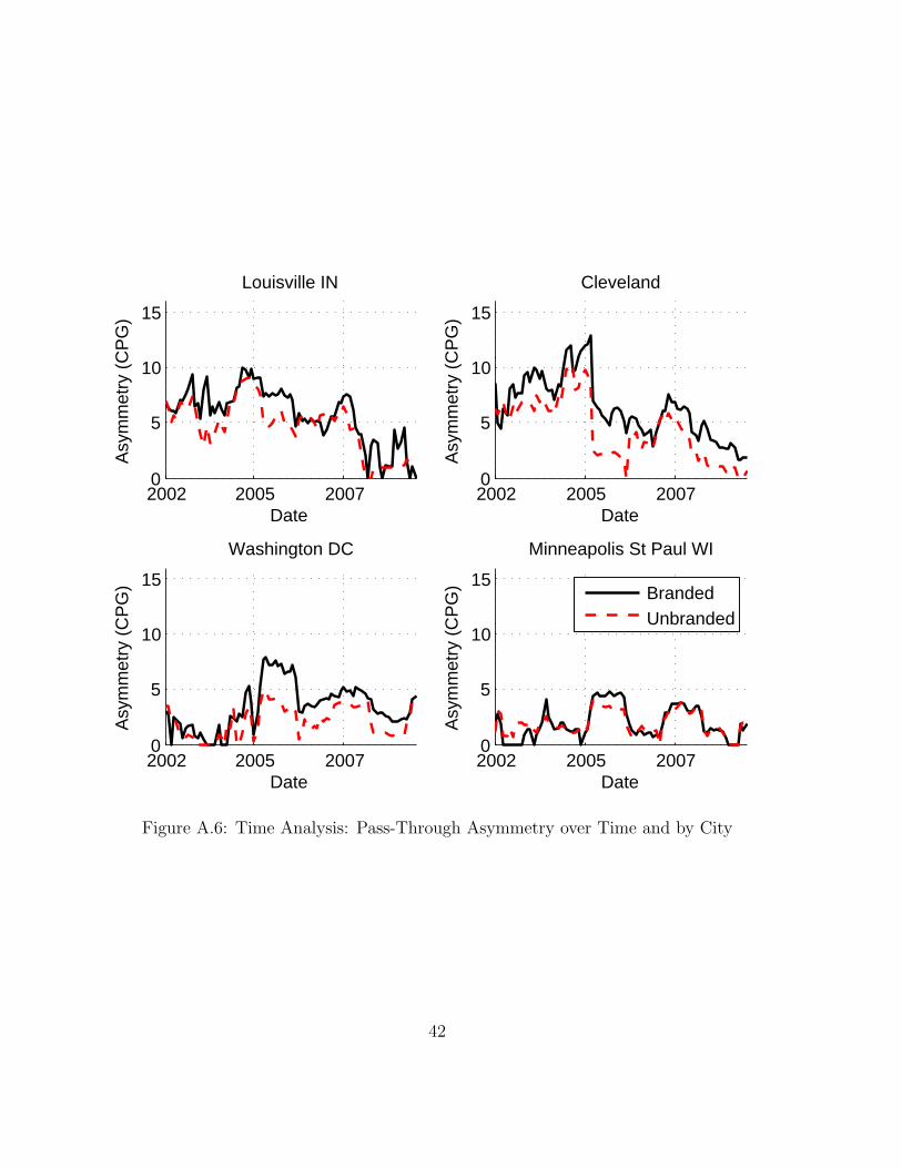
4.5 Differences Over Time
Finally, in figure 7 below and figure A.6 in the appendix, I investigate how pass-through
asymmetry has changed over time. For this analysis, I estimate my model at a daily
frequency for both branded and unbranded gasoline, but I run 80 separate overlapping
regressions on a 12-month window of data centered on each month in the data. I then
calculate the total loss due to asymmetry under the two regimes laid out above.
The asymmetry in pass-through from rack prices to retail prices varies significantly
from year to year and peaks in 2005, possibly because 2005 was the most active hurricane
season in history. In 2009, pass-through asymmetry cost consumers about 2 cpg on
branded gasoline and between 1 and 1.5 cpg on unbranded gasoline. This assumes that
consumers purchase their gas uniformly across all days no matter if prices are rising or
falling.
26
1- - - 1
~r:i E 1- E"I;l, I 'I ' I I '1' I I
'!

Jan02 Jan04 Jan06 Jan08 Jan100
0.5
1
1.5
2
2.5
3
3.5
4
4.5
5
Date
Asy
mm
etry
(C
PG
)
Asymmetry Over Time, Rolling 12−Month RegressionsAll City Specification
Rack to Retail
BrandedUnbranded
Figure 7: Time Analysis: Pass-Through Asymmetry by Year, National
4.6 Formal Tests of Asymmetry
In order to formally test for asymmetry, I report F-statistics for the pattern asymmetry
in equation 6. I test the following hypothesis:
H0 : β+1i = β−
1i ∀ i
H1 : β+1i 6= β−
1i for some i.
Note this is a two-sided test, so includes the possibility that the asymmetry is both the
rockets and feather type and the opposite. To implement the test, I save the residual sum
of squares, RSSu, from the full (unrestricted) model where the coefficients are allowed to
vary separately for positive and negative shocks. I then estimate a symmetric (restricted)
27

model, with only one set of β1i coefficients and save RSSr. Note that minimizing the
BIC separately for each model would mean that a different number of lags is included in
each.21 Therefore, I again restrict the number of lags to be 14 days in both regressions
so the only difference between the models is the restriction on the parameters. Formally,
the test statistic is of the usual form:
F̃ =(RSSr − RSSu)/(Ku − Kr)
RSSu/(N − Ku), (9)
where Ku and Kr are the number of parameters to be estimated in the unrestricted and
restricted models respectively. Results are reported in tables 7, 8, and 9 below.
The statistics reported in the tables largely confirm what has been shown in the im-
pulse response functions in the previous sections. There is strong evidence of asymmetry,
both in each city separately and in the all-city specification, in rack to retail prices and
spot to rack prices. The evidence is less strong when the upstream price is the crude
oil price. The branded rack to retail price relationship again show stronger evidence of
asymmetry compared with unbranded rack to retail prices.
The year-by-year regressions reveal some interesting patterns. Though the complete-
year regressions show pattern asymmetry in San Francisco for branded rack to retail
prices, the F-statistics for the individual year regressions are almost never significant.
The branded rack to retail regressions for 2009 alone only show evidence of asymmetry in
17 of the 27 metro areas, though the complete-year regressions show strong asymmetry
in 26 of the 27 metro areas. Thus, one implication is that studies which rely on shorter
samples may not find evidence of asymmetry, when it does exist. Further investigation is
required to determine what types of shocks (day-to-day movements versus large changes)
are driving the asymmetric results over the entire sample.
21See Ye, et. al. (2005) for a discussion of this issue.
28

Atlanta 3.33*** 4.45*** 2.00*** 2.67*** 12.53*** 21.35*** 17.74***Boston 3.63*** 3.69*** 2.18*** 5.34*** 4.45*** 16.08*** 12.45***Chicago 2.78*** 2.66*** 1.82** 16.83*** 14.20*** 8.47*** 6.52***Cleveland 3.36*** 4.05*** 1.58** 2.43*** 3.84*** 7.63*** 6.72***Dallas 5.39*** 3.68*** 3.10*** 16.79*** 18.73*** 15.54*** 12.05***Denver 2.52*** 3.01*** 1.16 10.18*** 6.44*** 8.33*** 6.29***Detroit 3.36*** 1.83** 1.77** 4.37*** 4.46*** 24.57*** 15.28***Washington DC 4.22*** 4.63*** 1.78** 16.43*** 21.34*** 15.49*** 13.21***Washington MD 4.22*** 4.63*** 3.26*** 16.43*** 21.34*** 18.71*** 15.42***Washington VA 4.22*** 4.63*** 1.55* 16.43*** 21.34*** 21.98*** 20.22***Washington WV 4.10*** 4.50*** 1.58** 3.49*** 3.77*** 3.32*** 5.54***Houston 4.89*** 5.23*** 2.53*** 17.31*** 10.04*** 24.12*** 12.32***Los Angeles 3.87*** 2.35*** 1.05 0.76 2.76*** 9.34*** 1.81**Louisville IN 4.52*** 4.09*** 1.35 4.21*** 1.86** 7.60*** 6.69***Louisville KY 3.73*** 4.24*** 2.08*** 19.47*** 20.61*** 5.64*** 6.92***Miami 3.91*** 3.28*** 2.07*** 1.81** 11.96*** 19.75*** 10.55***Minneapolis St Paul MN 2.76*** 3.67*** 1.41 10.02*** 3.88*** 9.91*** 9.18***Minneapolis St Paul WI 2.76*** 3.67*** 4.80*** 10.02*** 3.88*** 7.54*** 6.38***New Orleans 5.88*** 4.25*** 2.19*** 3.48*** 7.59*** 11.35*** 4.77***Newark 3.32*** 3.04*** 3.14*** 4.71*** 2.93*** 24.87*** 14.91***New York 3.32*** 3.04*** 2.60*** 4.71*** 2.93*** 13.13*** 7.70***Phoenix 1.53* 3.79*** 1.43* 2.21*** 1.78** 3.84*** 3.67***Salt Lake City 3.56*** 3.88*** 1.35 1.68** 1.11 11.81*** 7.20***San Francisco 2.72*** 2.11*** 0.81 1.19 2.07*** 3.75*** 0.99Seattle 3.70*** 3.10*** 1.06 2.65*** 3.06*** 10.25*** 4.07***St Louis IL 3.97*** 2.33*** 1.49* 4.86*** 4.32*** 6.36*** 6.47***St Louis MO 3.05*** 6.33*** 1.43* 16.08*** 14.56*** 7.41*** 5.73***All City Regression 69.58*** 54.68*** 240.65*** 193.75*** 192.97*** 155.39*** 86.97***
Branded Rack to Retail
Unbranded Rack to Retail
WTI to Branded Rack
WTI to Unbranded
RackWTI to Retail
Spot to Branded Rack
Spot to Unbranded
Rack
Significance at the 1% (***), 5% (**), and 10% (**) levels.
Table 7: F-Statistics On the Existence of Pattern Asymmetry (All Years)
5 Conclusion and Future Work
The purpose of this study was to understand why so many researchers have studied
asymmetric pass-through in the gasoline industry and have come to varying conclusions.
Many of the discrepancies can be explained by variations in the data and the model
specification. I found that pass-through asymmetries do exist in wholesale rack to retail
prices as well as in spot to retail prices, but the asymmetry is weak to non-existent in
other price relationships.22 Pass-through asymmetry in the branded wholesale to retail
price relationship was shown to be larger than its unbranded counterpart. Averaging
22In some cases, I find evidence of prices rising slower than they fall, however the magnitude of thisasymmetry is relatively small.
29

Atlanta 1.50* 1.96*** 1.70** 7.17*** 1.33 2.14*** 4.22*** 2.02***Boston 1.80** 5.07*** 0.88 4.80*** 1.55* 3.31*** 1.55* 2.15***Chicago 1.10 1.60** 1.56* 2.06*** 1.41 3.13*** 2.01*** 2.11***Cleveland 1.05 2.05*** 2.56*** 1.50* 1.17 1.92*** 1.97*** 1.80**Dallas 2.72*** 1.48* 2.08*** 4.34*** 1.70** 3.49*** 2.53*** 2.15***Denver 1.28 1.30 1.06 3.83*** 1.51* 1.42 0.95 1.83**Detroit 0.82 1.04 3.39*** 4.97*** 3.43*** 3.22*** 4.49*** 2.27***Washington DC 0.49 1.11 1.08 5.47*** 1.32 1.83** 2.65*** 1.39Washington MD 2.40*** 1.73** 1.72** 5.29*** 2.65*** 2.20*** 3.69*** 2.01***Washington VA 1.62** 1.64** 2.25*** 6.16*** 2.83*** 2.97*** 3.28*** 2.25***Washington WV 1.13 1.50* 1.27 2.74*** 0.69 1.70** 1.30 1.82**Houston 2.02*** 2.21*** 2.31*** 7.18*** 2.65*** 5.54*** 4.74*** 3.79***Los Angeles 1.40 2.30*** 2.55*** 1.69** 1.24 2.36*** 2.34*** 1.37Louisville IN 1.69** 0.80 1.67** 3.32*** 1.35 1.96*** 2.01*** 0.68Louisville KY 0.82 0.76 1.33 3.03*** 1.56* 1.47* 1.11 1.26Miami 2.04*** 2.31*** 0.67 3.13*** 4.76*** 4.63*** 2.38*** 5.76***Minneapolis St Paul MN 1.75** 0.71 2.53*** 1.99*** 2.92*** 3.61*** 2.08*** 1.36Minneapolis St Paul WI 2.06*** 1.59** 2.50*** 4.23*** 2.14*** 1.83** 1.19 1.13New Orleans 1.49* 1.32 3.56*** 2.06*** 3.05*** 3.07*** 1.75** 2.70***Newark 1.06 4.74*** 1.09 6.33*** 2.90*** 2.16*** 2.48*** 2.28***New York 0.85 3.70*** 1.41 3.44*** 1.68** 2.35*** 1.44* 1.30Phoenix 1.91*** 1.67** 2.32*** 2.46*** 1.48* 1.05 0.96 0.82Salt Lake City 1.79** 1.73** 1.70** 3.61*** 4.18*** 1.71** 2.68*** 1.21San Francisco 0.95 1.03 1.85** 1.05 1.54* 0.58 0.87 1.03Seattle 2.27*** 2.86*** 2.83*** 1.48* 0.79 3.95*** 4.30*** 2.10***St Louis IL 1.78** 0.93 1.00 2.77*** 1.10 1.47* 2.07*** 1.20St Louis MO 1.86** 1.51* 0.68 2.66*** 1.69** 1.33 1.69** 1.93***All City Regression 4.77*** 7.71*** 13.81*** 47.00*** 14.25*** 16.00*** 27.08*** 10.57***
2009
Significance at the 1% (***), 5% (**), and 10% (**) levels.
2002 2003 2004 2005 2006 2007 2008
Table 8: F-Statistics, Branded Rack to Retail Prices (By Year)
daily data to obtain a weekly price series attenuates the findings of asymmetry as it
masks important day-to-day variation in prices.
Still, this leaves several open questions including why there are differences in the
pass-through asymmetry across cities and between branded and unbranded wholesale
gasoline. Research that has attempted to explain the asymmetry has focused on the
demand side, with consumer search cost and inventory management by drivers being the
leading explanations. Unless consumers vary across cities, supply-side factors could help
explain the geographic variation.
In future work, I will focus on which supply-side characteristics are associated with
30

Atlanta 0.96 1.68** 1.07 3.06*** 1.04 1.93*** 2.71*** 1.80**Boston 0.89 4.03*** 0.83 3.27*** 1.45* 1.63** 1.48* 1.99***Chicago 1.13 1.56* 1.32 2.43*** 0.85 3.16*** 2.01*** 1.53*Cleveland 0.84 1.78** 2.91*** 2.18*** 1.52* 1.42* 1.92*** 1.31Dallas 2.41*** 1.12 1.67** 3.72*** 1.65** 2.36*** 1.54* 2.14***Denver 1.30 0.60 1.36 4.14*** 1.14 1.65** 1.57** 1.31Detroit 0.72 1.55* 2.18*** 3.94*** 2.84*** 1.67** 3.05*** 0.80Washington DC 0.67 1.14 1.15 6.08*** 0.66 1.64** 0.87 1.50*Washington MD 1.55* 0.95 1.44* 5.59*** 1.58** 1.42 1.63** 1.80**Washington VA 1.14 0.83 2.09*** 11.14*** 2.40*** 1.74** 1.83** 1.67**Washington WV 1.28 1.20 1.85** 4.14*** 1.00 0.73 1.02 1.51*Houston 2.74*** 0.91 1.97*** 3.89*** 2.02*** 1.94*** 3.35*** 2.16***Los Angeles 1.08 1.27 1.42* 1.43* 1.11 1.08 2.07*** 1.31Louisville IN 1.25 0.98 2.54*** 5.51*** 1.31 1.19 1.27 1.08Louisville KY 1.78** 0.63 1.44* 4.13*** 1.57** 1.38 1.20 2.14***Miami 2.29*** 1.84** 0.50 1.74** 3.61*** 2.52*** 0.94 3.77***Minneapolis St Paul MN 1.58** 0.45 1.90*** 1.78** 2.47*** 3.24*** 2.12*** 1.00Minneapolis St Paul WI 1.61** 1.99*** 1.85** 1.78** 1.70** 1.09 1.15 1.18New Orleans 1.28 1.13 2.98*** 1.32 2.41*** 2.18*** 0.88 1.36Newark 0.85 3.83*** 0.70 3.39*** 0.67 1.82** 2.60*** 1.61**New York 0.52 2.49*** 1.00 3.70*** 0.86 2.19*** 1.00 1.21Phoenix 1.64** 1.23 0.64 4.10*** 1.76** 2.66*** 1.26 1.73**Salt Lake City 3.30*** 1.03 0.86 4.10*** 2.72*** 2.06*** 1.76** 0.92San Francisco 0.89 1.33 0.99 0.52 0.78 0.42 0.81 0.53Seattle 1.67** 2.01*** 1.70** 0.83 1.54* 1.88*** 1.38 1.11St Louis IL 1.16 0.84 0.94 1.97*** 1.32 1.72** 4.36*** 1.33St Louis MO 0.86 0.84 0.77 2.17*** 2.20*** 0.90 1.87** 2.28***All City Regression 3.19*** 4.66*** 11.33*** 33.01*** 7.06*** 8.48*** 15.08*** 5.30***
2002 2003 2004 2005 2006 2007 2008 2009
Significance at the 1% (***), 5% (**), and 10% (**) levels.
Table 9: F-Statistics, Unbranded Rack to Retail Prices (By Year)
more or less asymmetric pass-through. These may include differences in the retail own-
ership structure (e.g., a larger percentage of lessee-dealer owned stations versus inde-
pendents) similar to the study by Lewis (2009) and retail concentration similar to the
study by Deltas (2008). In addition, the results in this paper indicate that, at least
in some cities, pass-through asymmetry varies over time. Supply-side shocks caused by
hurricanes, pipeline disruptions, and refinery maintenance or outages, which only affect
certain geographic areas and vary from year to year, may provide an explanation.
31

References
[1] Bachmeier, Lance and James Griffin, (2003). “New Evidence on Asymmetric Gaso-
line Price Responses.” The Review of Economics and Statistics, 85(3), August 2003.
[2] Bacon, Robert W., (1991). “Rockets and Feathers: The Asymmetric Speed of Ad-
justment of UK Retail Gasoline Prices to Cost Changes.” Energy Economics, 13
July 1991.
[3] Borenstein, S., C. A. Cameron and R. Gilbert, (1997). “Do Gasoline Prices Respond
Asymmetrically to Crude Oil Price Changes?” Quarterly Journal of Economics,
112(1), 1997.
[4] Borenstein, S., (1991). “Selling Costs and Switching Costs: Explaining Retail Gaso-
line Margins.” The RAND Journal of Economics, 22(3), 1991.
[5] Borenstein, S., Andrea Shepard (1996). “Dynamic Pricing in Retail Gasoline Mar-
kets.” The RAND Journal of Economics, 27(3), 1996.
[6] Bulow, Jeremy and Paul Pfleiderer, (1983). “A Note on the Effect of Cost Changes
on Prices.” Journal of Political Economy, 91, 1983.
[7] Deltas, George (2008). “Retail Gasoline Price Dynamics and Local Market Power.”
The Journal of Industrial Economics, 61(3), September 2008.
[8] Eckert, Andrew (2002). “Retail Price Cycles and Response Asymmetry.” Canadian
Journal of Economics, 35(1), 2002.
[9] Energy Information Administration, US Department of Energy, (2007). “Refinery
Outages: Description and Potential Impact on Petroleum Product Prices.” March
2007.
32
[10] Energy Information Administration, US Department of Energy, (2008). “A Primer
on Gasoline Prices.” Online: http://www.eia.doe.gov/bookshelf/brochures/
gasolinepricesprimer/index.html [Downloaded: 09/11/2008], May 2008.
[11] Engle R. and C.W.J. Granger, (1987). “Co-Integration and Error Correction: Rep-
resentation, Estimation, and Testing.” Econometrica, 55(2), 1987.
[12] Espey, Molly, (1996). “Explaining Variation in Elasticity of Gasoline Demand in the
United States: A Meta Analysis.” The Energy Journal, 17, 1996.
[13] The Federal Trade Commission, (2006). “Investigation of Gasoline Price Manipula-
tion and Post-Katrina Gasoline Price Increases.” Spring 2006.
[14] The Federal Trade Commission, (2005). “Gasoline Price Changes:
The Dynamics of Supply, Demand and Competition.” Available at
http://www.ftc.gov/reports/gasprices05/050705gaspricesrpt.pdf, 2005.
[15] Godby, R, A.M. Lintner, T. Stengos, and B. Wandschneider, (2000). “Testing for
Asymmetric Pricing in the Canadian Retail Gasoline Market.” Energy Economics,
22, 2000.
[16] Goldberg, Pinelopi K. and Rebecca Hellerstein, (2008). “A Structural Approach to
Explaining Incomplete Exchange-Rate Pass-Through and Pricing-to-Market.” The
American Economic Review, 98(2), 2008.
[17] Goodwin, Barry, and Matthew Holt, (1999). “Price Transmission and Asymmetric
Adjustment in the U.S. Beef Sector.” American Journal of Agricultural Economics,
81, August 1999.
[18] The Government Accountability Office, (2006). “Energy Markets: Factors Con-
tributing to Higher Gasoline Prices.” GAO-06-412T. February 2006.
33

[19] Gron, Anne, Deborah Swenson, (2000). “Cost Pass-Through in the U.S. Automobile
Market.” The Review of Economics and Statistics, 82(2), 2000.
[20] Hastings, Justine, Jennifer Brown, Erin Mansur, and Sofia Villas-Boas, (2008). “Re-
formulating Competition? Gasoline Content Regulation and Wholesale Gasoline
Prices.” Journal of Environmental Economics and Management, January 2008.
[21] Hosken, Daniel, Robert McMillan and Christopher Taylor, (2008). “Retail Gasoline
Pricing: What Do We Know?” International Journal of Industrial Organization,
26(6), November 2008.
[22] Kim, Donghun and Ronald Cotterill, (2008). “Cost Pass-Through in Differentiated
Product Markets: The Case of U.S. Processed Cheese.” The Journal of Industrial
Economics, 60(1), March 2008.
[23] Knittel, Christopher, Jonathan E. Hughes, and Daniel Sperling, (2008). “Evidence of
a Shift in the Short-Run Price Elasticity of Gasoline Demand.” The Energy Journal,
29(1), January 2008.
[24] Lewis, Matt, (forthcoming). “Asymmetric Price Adjustment and Consumer Search:
an Examination of Retail Gasoline Market,” forthcoming in Journal of Economics
and Management Strategy.
[25] Lewis, Matt, and Michael Noel (forthcoming). “The Speed of Gasoline Price Re-
sponse in Markets with and without Edgeworth Cycles,” forthcoming in The Review
of Economic Studies.
[26] Lewis, Matt (2009). “Temporary Wholesale Gasoline Price Spikes have Long Lasting
Retail Effects: The Aftermath of Hurricane Rita.” Journal of Law and Economics,
52(3), 2009.
34

[27] Lidderdale, T.C.M. (United States Energy Information Administration), (1999).
“Environmental Regulations and Changes in Petroleum Refining Operations.” On-
line: http://www.eia.doe.gov/emeu/steo/pub/special/enviro.html [Down-
loaded: 12/07/2007], 1999.
[28] MacKinnon, James, (2010). “Critical Values for Cointegration Tests.” Queen’s Eco-
nomics Department Working Paper No. 1227. 2010.
[29] Noel, Michael D., (2007). “Edgeworth Price Cycles, Cost-Based Pricing, and Sticky
Pricing in Retail Gasoline Markets.” Review of Economics and Statistics, Vol. 89,
2007.
[30] Peterson, D. J. and Sergej Mahnovski, (2003). “New Forces at Work in Refining:
Industry Views of Critical Business and Operations Trends.” Santa Monica, CA :
RAND, 2003.
[31] The United States Senate, (2002). “Gas Prices: How are they Really Set?”
Online: http://www.senate.gov/~gov_affairs/042902gasreport.htm [Down-
loaded 10/01/2007], May 2002.
[32] Ten Kate, Adriaan and Gunnar Niels, (2005). “To What Extent are Cost Savings
Passed on to Consumers? An Oligopoly Approach.” European Journal of Law and
Economics, 20, 2005.
[33] Ye, Michael, John Zyren, Joanne Shore, and Michael Burdette, (2005). “Regional
Comparisons, Spatial Aggregation, and Asymmetry of Price Pass-Through in U.S.
Gasoline Markets.” Atlantic Economic Journal, 33, 2005.
35

A Appendix
!!!!!
!
!!
!
!
!!!
!
!!!
!
!!
!
!
!
!
!
!
!
!!!!
!
!!
!
!
!!!!!!!!!
!!
!!!
!
!
!
!
!
!
!
!
!
!
!
!
!!!!!
!
!!!!!!!!
!!!!!!!!!
!
!
!!
!
!
!
!
!
!
!
!!
!
!
!
!
!
!
!
!
!
!
!
!
!!
!
!
!
!!!!
!
"
"
"
"
Belle
DECATUR
Cahokia
Hartford
St. Louis
St. Peters Wood River Refinery
Jefferson City
CAPE GIRARDEAU
" Refinery! Refined Products Terminal
St. Louis MSAIllinoisMissouri
St. Louis MSA
Illinois
Missouri
Figure A.1: St. Louis Retail Market Areas.
36

Parameter Estimate Standard ErrorConstant -0.087*** 0.011+ (Rack(t) - Rack(t-1)) 0.274*** 0.004+ (Rack(t-1) - Rack(t-2)) 0.101*** 0.004+ (Rack(t-2) - Rack(t-3)) 0.059*** 0.004+ (Rack(t-3) - Rack(t-4)) 0.036*** 0.004+ (Rack(t-4) - Rack(t-5)) 0.052*** 0.004+ (Rack(t-5) - Rack(t-6)) 0.044*** 0.004- (Rack(t) - Rack(t-1)) 0.068*** 0.004- (Rack(t-1) - Rack(t-2)) 0.085*** 0.004- (Rack(t-2) - Rack(t-3)) 0.056*** 0.004- (Rack(t-3) - Rack(t-4)) 0.075*** 0.004+ (Retail(t-1) - Retail(t-2)) 0.335*** 0.005+ (Retail(t-2) - Retail(t-3)) -0.244*** 0.005- (Retail(t-1) - Retail(t-2)) 0.328*** 0.012- (Retail(t-2) - Retail(t-3)) 0.101*** 0.013- (Retail(t-3) - Retail(t-4)) -0.025** 0.012- (Retail(t-4) - Retail(t-5)) 0.011 0.012- (Retail(t-5) - Retail(t-6)) 0.132*** 0.011+ EC Term -0.021*** 0.001- EC Term -0.059*** 0.002NR2
Durbin-Watson Statistic
54,530
2.0200.45
Dependent Variable: Retail(t) - Retail(t-1). City-level fixed effects included in the first-stage regression. ***, **, * significant at the 1%, 5% and 10% levels respectively.
Table A.1: Regression Results: Branded Rack to Retail Prices, All Cities Included
37

0 2 4 6 8 10 12 14 16 18 200
5
10
15
Days Since Upstream Price Shock
Cha
nge
in D
owns
trea
m P
rice
(Cen
ts/G
allo
n)
Impulse Response:WTI to Gasoline Spot, National10 Cent/Gallon Upstream Shock
Positive Shock+95 CI−95 CINegative Shock+95 CI−95 CI
Figure A.2: Impulse Response Function: Crude Oil to Gasoline Spot Prices, All CitiesIncluded
38

0 2 4 6 8 10 12 14 16 18 200
5
10
15
Days Since Upstream Price Shock
Cha
nge
in D
owns
trea
m P
rice
(Cen
ts/G
allo
n)
Impulse Response:WTI to Branded Rack, National10 Cent/Gallon Upstream Shock
Positive Shock+95 CI−95 CINegative Shock+95 CI−95 CI
Figure A.3: Impulse Response Function: Crude Oil to Rack Prices, All Cities Included
39
0 2 4 6 8 10 12 14 16 18 200
5
10
15
Days Since Upstream Price Shock
Cha
nge
in D
owns
trea
m P
rice
(Cen
ts/G
allo
n)
Impulse Response:WTI to Retail, National
10 Cent/Gallon Upstream Shock
Positive Shock+95 CI−95 CINegative Shock+95 CI−95 CI
Figure A.4: Impulse Response Function: Crude Oil to Retail Prices, All Cities Included
40

0 2 4 6 8 10 12 14 16 18 200
5
10
15
Days Since Upstream Price Shock
Cha
nge
in D
owns
trea
m P
rice
(Cen
ts/G
allo
n)
Impulse Response:Spot to Branded Rack, National10 Cent/Gallon Upstream Shock
Positive Shock+95 CI−95 CINegative Shock+95 CI−95 CI
Figure A.5: Impulse Response Function: Gasoline Spot to Rack, All Cities Included
41
2002 2005 20070
5
10
15
Date
Asy
mm
etry
(C
PG
)
Louisville IN
2002 2005 20070
5
10
15
Date
Asy
mm
etry
(C
PG
)
Cleveland
2002 2005 20070
5
10
15
Date
Asy
mm
etry
(C
PG
)
Washington DC
2002 2005 20070
5
10
15
Date
Asy
mm
etry
(C
PG
)
Minneapolis St Paul WI
BrandedUnbranded
Figure A.6: Time Analysis: Pass-Through Asymmetry over Time and by City
42