A&A 586, A134 (2016)DOI: 10.1051/0004-6361/201425022c© ESO 2016

Astronomy&

Astrophysics

Planck intermediate resultsXXXI. Microwave survey of Galactic supernova remnants

Planck Collaboration: M. Arnaud67, M. Ashdown63,5, F. Atrio-Barandela17, J. Aumont54, C. Baccigalupi82,A. J. Banday88,10, R. B. Barreiro59, E. Battaner90,91, K. Benabed55,87, A. Benoit-Lévy22,55,87, J.-P. Bernard88,10,

M. Bersanelli30,46, P. Bielewicz77,10,82, J. Bobin67, J. R. Bond9, J. Borrill13,85, F. R. Bouchet55,84, C. L. Brogan75,C. Burigana45,28,47, J.-F. Cardoso68,1,55, A. Catalano69,66, A. Chamballu67,14,54, H. C. Chiang25,6, P. R. Christensen78,33,

S. Colombi55,87, L. P. L. Colombo21,61, B. P. Crill61,11, A. Curto59,5,63, F. Cuttaia45, R. D. Davies62, R. J. Davis62,P. de Bernardis29, A. de Rosa45, G. de Zotti42,82, J. Delabrouille1, F.-X. Désert50,51, C. Dickinson62, J. M. Diego59,S. Donzelli46, O. Doré61,11, X. Dupac36, T. A. Enßlin73, H. K. Eriksen58, F. Finelli45,47, O. Forni88,10, M. Frailis44,

A. A. Fraisse25, E. Franceschi45, S. Galeotta44, K. Ganga1, M. Giard88,10, Y. Giraud-Héraud1, J. González-Nuevo18,59 ,K. M. Górski61,92, A. Gregorio31,44,49, A. Gruppuso45, F. K. Hansen58, D. L. Harrison57,63,

C. Hernández-Monteagudo12,73 , D. Herranz59, S. R. Hildebrandt61,11, M. Hobson5, W. A. Holmes61,K. M. Huffenberger23, A. H. Jaffe52, T. R. Jaffe88,10, E. Keihänen24, R. Keskitalo13, T. S. Kisner71, R. Kneissl35,7,

J. Knoche73, M. Kunz16,54,3, H. Kurki-Suonio24,40, A. Lähteenmäki2,40, J.-M. Lamarre66, A. Lasenby5,63,C. R. Lawrence61, R. Leonardi8, M. Liguori27,60, P. B. Lilje58, M. Linden-Vørnle15, M. López-Caniego36,59,

P. M. Lubin26, D. Maino30,46, M. Maris44, D. J. Marshall67, P. G. Martin9, E. Martínez-González59 , S. Masi29,S. Matarrese27,60,39, P. Mazzotta32, A. Melchiorri29,48, L. Mendes36, A. Mennella30,46, M. Migliaccio57,63,M.-A. Miville-Deschênes54,9 , A. Moneti55, L. Montier88,10, G. Morgante45, D. Mortlock52, D. Munshi83,J. A. Murphy76, P. Naselsky79,34, F. Nati25, F. Noviello62, D. Novikov72, I. Novikov78,72, N. Oppermann9,

C. A. Oxborrow15, L. Pagano29,48, F. Pajot54, R. Paladini53, F. Pasian44, M. Peel62, O. Perdereau65, F. Perrotta82,F. Piacentini29, M. Piat1, D. Pietrobon61, S. Plaszczynski65, E. Pointecouteau88,10 , G. Polenta4,43, L. Popa56,

G. W. Pratt67, J.-L. Puget54, J. P. Rachen19,73, W. T. Reach89 ,�, W. Reich74, M. Reinecke73, M. Remazeilles62,54,1,C. Renault69, J. Rho81, S. Ricciardi45, T. Riller73, I. Ristorcelli88,10, G. Rocha61,11, C. Rosset1, G. Roudier1,66,61,

B. Rusholme53, M. Sandri45, G. Savini80, D. Scott20, V. Stolyarov5,86,64, D. Sutton57,63, A.-S. Suur-Uski24,40,J.-F. Sygnet55, J. A. Tauber37, L. Terenzi38,45, L. Toffolatti18,59,45, M. Tomasi30,46, M. Tristram65, M. Tucci16,G. Umana41, L. Valenziano45, J. Valiviita24,40, B. Van Tent70, P. Vielva59, F. Villa45, L. A. Wade61, D. Yvon14,

A. Zacchei44, and A. Zonca26

(Affiliations can be found after the references)

Received 17 September 2014 / Accepted 24 November 2015

ABSTRACT

The all-sky Planck survey in 9 frequency bands was used to search for emission from all 274 known Galactic supernova remnants. Of these,16 were detected in at least two Planck frequencies. The radio-through-microwave spectral energy distributions were compiled to determine themechanism for microwave emission. In only one case, IC 443, is there high-frequency emission clearly from dust associated with the supernovaremnant. In all cases, the low-frequency emission is from synchrotron radiation. As predicted for a population of relativistic particles with energydistribution that extends continuously to high energies, a single power law is evident for many sources, including the Crab and PKS 1209-51/52.A decrease in flux density relative to the extrapolation of radio emission is evident in several sources. Their spectral energy distributions can beapproximated as broken power laws, S ν ∝ ν−α, with the spectral index, α, increasing by 0.5–1 above a break frequency in the range 10–60 GHz.The break could be due to synchrotron losses.

Key words. ISM: supernova remnants – cosmic rays – radio continuum: ISM

1. Introduction

Supernovae leave behind remnants that take on several forms(McCray & Wang 1996). The core of the star that explodes iseither flung out with the rest of the ejecta into the surroundingmedium (in the case of a Type I supernova), or it survives as a

� Corresponding author: W. T. Reach, wreach@sofia.usra.edu

neutron star or black hole (in the case of a Type II supernova).The neutron stars eject relativistic particles from jets, makingthem visible as pulsars and powering wind nebulae. These windnebulae are sometimes called “plerions” and are exemplified bythe Crab Nebula. Ejecta from the stellar explosion are only visi-ble for young (∼103 yr) supernova remnants (SNRs), before theyare mixed with surrounding interstellar or residual circumstellar

Article published by EDP Sciences A134, page 1 of 21

A&A 586, A134 (2016)

material; such objects are exemplified by the historical Tychoand Kepler supernova remnants and Cassiopeia A. Type I su-pernovae from white dwarf deflagration leave behind supernovaremnants because their blast waves propagate into the interstellarmedium. Most supernova remnants are from older explosions,and the material being observed is interstellar (and circumstellarin some cases) material shocked by the supernova blast waves.The magnetic field of the medium is enhanced in the compressedpost-shock gas, and charged particles are accelerated to relativis-tic speeds, generating copious synchrotron emission that is thehallmark of a supernova remnant at radio frequencies.

At the highest radio frequencies and in the microwave, su-pernova remnants may transition from synchrotron emission toother mechanisms. The synchrotron brightness decreases as fre-quencies increase, and free-free emission (with its flatter spec-trum) and dust emission (with its steeply rising spectrum) willgain prominence. Dipole radiation from spinning dust grainscould possibly contribute (Scaife et al. 2007). Because the syn-chrotron radiation itself is an energy loss mechanism, the elec-trons decrease in energy over time, and relatively fewer higher-energy electrons should exist as the remnants age; therefore, thesynchrotron emission will diminish at higher frequencies. Forthese reasons, a survey of supernova remnants at microwave fre-quencies could reveal some keys to the evolution of relativisticparticles as they are produced and injected into the interstellarmedium, as well as potentially unveiling new emission mecha-nisms that can trace the nature of the older supernova remnants.

2. Observations

2.1. Properties of the Planck survey

Planck1 (Tauber et al. 2010; Planck Collaboration I 2011) is thethird generation space mission to measure the anisotropy of thecosmic microwave background (CMB). It observed the sky innine frequency bands covering 30–857 GHz with high sensitiv-ity and angular resolution from 31′ to 5′. The Low FrequencyInstrument (LFI; Mandolesi et al. 2010; Bersanelli et al. 2010;Mennella et al. 2011) covers the 30, 44, and 70 GHz bandswith amplifiers cooled to 20 K. The High Frequency Instrument(HFI; Lamarre et al. 2010; Planck HFI Core Team 2011a) coversthe 100, 143, 217, 353, 545, and 857 GHz bands with bolometerscooled to 0.1 K. A combination of radiative cooling and threemechanical coolers produces the temperatures needed for the de-tectors and optics (Planck Collaboration II 2011). Two data pro-cessing centres (DPCs) check and calibrate the data and makemaps of the sky (Planck HFI Core Team 2011b; Zacchei et al.2011; Planck Collaboration V 2014; Planck Collaboration VIII2014). Planck’s sensitivity, angular resolution, and frequencycoverage make it a powerful instrument for Galactic and extra-galactic astrophysics as well as cosmology. Early astrophysicsresults are given in Planck Collaboration VIII–XXVI 2011,based on data taken between 13 August 2009 and 7 June 2010.Intermediate astrophysics results are being presented in a se-ries of papers based on data taken between 13 August 2009and 27 November 2010.

1 Planck (http://www.esa.int/Planck) is a project of theEuropean Space Agency (ESA) with instruments provided by two sci-entific consortia funded by ESA member states and led by PrincipalInvestigators from France and Italy, telescope reflectors providedthrough a collaboration between ESA and a scientific consortium ledand funded by Denmark, and additional contributions from NASA(USA).

Table 1. Planck survey properties.

Center Beam Calibration Unitsfrequency FWHMa accuracyb factorc

Band [GHz] [arcmin] [%] [Jy pix−1]

30 . . . . . . . 28.5 32.3 0.25 27.0044 . . . . . . . 44.1 27.1 0.25 56.5670 . . . . . . . 70.3 13.3 0.25 128.4

100 . . . . . . . 100 9.66 0.6 59.72143 . . . . . . . 143 7.27 0.5 95.09217 . . . . . . . 217 5.01 0.7 121.2353 . . . . . . . 353 4.86 2.5 74.63545 . . . . . . . 545 4.84 5 0.250857 . . . . . . . 857 4.63 5 0.250

Notes. (a) Beams are from Planck Collaboration VII (2014) for HFI andPlanck Collaboration IV (2014) for LFI. (b) Calibration is from PlanckCollaboration VIII (2014) for HFI and Planck Collaboration V (2014)for LFI. (c) Pixel sizes refer to the all-sky Healpix maps and are 11.8′for frequencies 30–70 GHz and 2.9′ for frequencies 100–857 GHz.

Relevant properties of Planck are summarized for each fre-quency band in Table 1. The effective beam shapes vary acrossthe sky and with data selection. Details are given in PlanckCollaboration IV (2014) and Planck Collaboration VII (2014).Average beam sizes are given in Table 1. Calibration of thebrightness scale was achieved by measuring the amplitude of thedipole of the cosmic microwave background (CMB) radiation,which has a known spatial and spectral form; this calibrationwas used for the seven lower frequency bands (30–353 GHz). Atthe two high frequencies (545 and 857 GHz), the CMB signal isrelatively low, so calibration was performed using measurementsof Uranus and Neptune. The accuracy of the calibration is givenin Table 1; the Planck calibration is precise enough that it is notan issue for the results discussed in this paper.

The Planck image products are at Healpix (Górski et al.2005) Nside = 2048 for frequencies 100–857 GHz and Nside =1024 for frequencies 30–70 GHz, in units of CMB thermody-namic temperature up to 353 GHz. For astronomical use, thetemperature units are converted to flux density per pixel by mul-tiplication by the factor given in the last column of Table 1.At 545 and 857 GHz, the maps are provided in MJy sr−1 units,and the scaling simply reflects the pixel size.

2.2. Flux density measurements

Flux densities were measured using circular aperture photom-etry. Other approaches to measuring the source fluxes wereexplored and could be pursued by future investigators. This in-cludes model fitting (e.g. Gaussian or other source shape moti-vated by morphology seen at other wavelengths convolved withthe beam) or non-circular aperture photometry (e.g. drawing ashape around the source and hand-selecting a background). Weexperimented with both methods and found they were highly de-pendent upon the choices made. The circular-aperture methodused in this paper has the advantages of being symmetric aboutthe source center (hence, eliminating all linear gradients in thebackground) as well as being objective about the shape ofthe source (hence, independent of assumptions about the mi-crowave emitting region).

Because of the wide range of Planck beam sizes and thecomparable size of the supernova remnants (SNRs), we tookcare to adjust the aperture sizes as a function of frequency and toscale the results to a flux density scale. For each SNR, the source

A134, page 2 of 21

Planck Collaboration: Planck supernova remnant survey

Table 2. Properties of detected supernova remnants.

Supernova remnant Angulara S 1 GHza Spectrala Notesb

diameter (′) (Jy) index

G21.5-0.9 G21.5-0.9 . . . . . . . . . . . . . 4 7 0.00 <103 yr, pulsarG34.7-0.4 W 44 . . . . . . . . . . . . . . . . . 35 230 0.37 2 × 104 yr, denseG69.0+2.7 CTB 80 . . . . . . . . . . . . . . . 80 120 . . . 105 yr, pulsar, plerionG74.0-8.5 Cygnus Loop . . . . . . . . . . . 230 210 . . . matureG89.0+4.7 HB 21 . . . . . . . . . . . . . . . . 120 220 0.38 5000 yr, denseG111.7-2.1 Cas A . . . . . . . . . . . . . . . . 5 2720 0.77 330 yr, ejecta, CCOG120.1+1.4 Tycho . . . . . . . . . . . . . . . . 8 56 0.65 young, Type IaG130.7+3.1 3C 58 . . . . . . . . . . . . . . . . 9 33 0.07 830 yr, plerion, pulsarG184.6-5.8 Crab . . . . . . . . . . . . . . . . . 7 1040 0.30 958 yr, plerion, pulsarG189.1+3.0 IC 443 . . . . . . . . . . . . . . . . 40 160 0.36 3 × 104 yr, dense ISM, CCOG260.4-3.4 Puppis A . . . . . . . . . . . . . . 60 130 0.50 CCO, 3700 yrG263.9-3.3 Vela . . . . . . . . . . . . . . . . . 255 1750 . . . 104 yrG296.5+10.0 PKS 1209-51/52 . . . . . . . . . 90 48 0.5 ∼104 yrG315.4-2.3 RCW 86 . . . . . . . . . . . . . . 42 49 0.60 1800 yrG326.3-1.8 MSH 15-56 . . . . . . . . . . . . 38 145 . . .G327.6+14.6 SN 1006 . . . . . . . . . . . . . . 30 19 0.60 1008 yr, Type Ia

Notes. (a) Flux densities at 1 GHz, radio spectral indices, and angular diameters are from Green (2009). For cases of unknown or strongly-spatially-variable spectral index, we put “. . .” in the table and use a nominal value of 0.5 in the figures for illustration purposes only. (b) Notes onthe properties of the SNR, gleaned from the Green (2009) catalogue and references therein, as well as updates from the online version http://www.mrao.cam.ac.uk/projects/surveys/snrs/. Plerion: radio emission is centre-filled. Pulsar: a pulsar is associated with the SNR. CCO: acentral compact object (presumably a neutron star) is associated with the supernova remnant from high-energy images. Dense ISM: the supernovaremnant is interacting with a dense interstellar medium. Xyr: estimated age of the supernova remnant. Mature: age likely greater than 105 yr. TypeX: the supernova that produced this supernova remnant was of type X.

size in the maps was taken to be the combination of the intrin-sic source size from the Green catalogue (Green 2009), θSNR inTable 2, and the Planck beam size, θb in Table 1:

θs =√θ2SNR + θ

2b. (1)

The flux densities were measured using standard aperture pho-tometry, with the aperture size centred on each target with a di-ameter scaled to θap = 1.5θs. The background was determined inan annulus of inner and outer radii 1.5θap and 2θap. To correctfor loss of flux density outside of the aperture, an aperture cor-rection as predicted for a Gaussian flux density distribution withsize θs was applied to each measurement:

fA =1

f (θap) − [ f (θout) − f (θin)] (2)

where the flux density enclosed within a given aperture is

f (θ) = 1 − e−4 ln 2(θ/θs)2(3)

and θin and θout are the inner and outer radii of annuluswithin which the background is measured. For the well-resolvedsources (diameter 50% larger than the beam FWHM), no aper-ture correction was applied. Aperture corrections are typi-cally 1.5 for the compact sources and by definition unity for thelarge sources. The use of a Gaussian source model for the inter-mediate cases (source comparable to beam) is not strictly appro-priate for SNRs, which are often limb-brightened (shell-like), sothe aperture corrections are only good to about 20%.

The uncertainties for the flux densities are a root-sum-squareof the calibration uncertainty (from Table 1) and the propagatedstatistical uncertainties. The statistical uncertainties (technically,appropriate for white uncorrelated noise only) take into accountthe number of pixels in the on-source aperture and background

annulus and using the robust standard deviation within the back-ground annulus to estimate the pixel-to-pixel noise for eachsource. The measurements are made using the native Healpixmaps, by searching for pixels within the appropriate aperturesand background annuli and calculating the sums and robust me-dians, respectively. This procedure avoids the need of generat-ing extra projections and maintains the native pixelization of thesurvey.

We verify the flux calibration scale by using the proceduredescribed above on the well-measured Crab Nebula. The fluxdensities are compared to previous measurements in Fig. 1. Thegood agreement verifies the measurement procedure used forthis survey, at least for a compact source. The Planck EarlyRelease Compact Source Catalogue (Planck Collaboration VII2011, hereafter ERCSC) flux density measurements for the Crabare lower than those determined in this paper, due to the sourcebeing marginally resolved by Planck at high frequencies.

Table 2 lists the basic properties of SNRs that were detectedby Planck. Table 3 summarises the Planck flux-density measure-ments for detected SNRs. To be considered a detection, eachSNR must have a statistically significant flux density measure-ment (flux density greater than 3.5 times the statistical uncer-tainty in the aperture photometry measurement) and be evidentby eye for at least two Planck frequencies. Inspection of thehigher-frequency images allows for identification of interstellarforegrounds for the supernova remnants, which are almost allbest-detected at the lowest frequencies. A large fraction of theSNRs are located close to the Galactic plane and are smallerthan the low-frequency Planck beam. Essentially none of thosetargets could be detected with Planck due to confusion from sur-rounding H ii regions. Dust and free-free emission from H ii re-gions makes them extremely bright at far-infrared wavelengthsand moderately bright at radio frequencies. Supernova remnantsin the Galactic plane would only be separable from H ii re-gions using a multi-frequency approach and angular resolution

A134, page 3 of 21

A&A 586, A134 (2016)

Fig. 1. Top: Planck Images of the Crab nebula at frequencies increasingfrom 30 GHz at top left to 857 GHz at bottom right. Each image is 100′on a side, with the three lowest-frequency images smoothed by 7′.Bottom: microwave spectral energy distribution of the Crab Nebula.Filled circles are Planck measurements with 3σ error bars. The opensymbol at 1 GHz and the dashed line emanating from it are the fluxand power law with spectral index from the Green catalogue. Open dia-monds are from the compilation of flux densities by Macías-Pérez et al.(2010).

significantly higher than Planck. More detailed results from theflux measurements are provided in the Appendix.

As a test of the quality of the results and robustness to con-tamination from the CMB, we performed the flux density mea-surements using the total intensity maps as well as the CMB-subtracted maps. Differences greater than 1σ were seen onlyfor the largest SNRs. Of the measurements in Table 3, onlythe following flux densities were affected at the 2σ or greaterlevel: Cygnus Loop (44 and 70 GHz), HB 21 (70 GHz), and Vela(70 GHz).

3. Results and discussion of individual objects

The images and spectral energy distributions (SEDs) of detectedSNRs are summarized in the following subsections. A goal ofthe survey is to determine whether new emission mechanisms orchanges in the radio emission mechanisms are detected in themicrowave range. Therefore, for each target, the 1 GHz radioflux density (Green 2009) was used to extrapolate to microwavefrequencies using a power law. The extrapolation illustratesthe expected Planck flux densities, if synchrotron radiation isthe sole source of emission and the high-energy particles havea power-law energy distribution. The Green (2009) SNR cata-logue was compiled from an extensive and continuously updatedliterature search. The radio spectral indices are gleaned fromthat same compendium. They represent a fit to the flux densi-ties from 0.4 to 5 GHz, where available, and are the value α ina SED S ν = S ν(1 GHz)ν−αGHz. The spectral indices can be quiteuncertain in some cases, where observations with very differentobserving techniques are combined (in particular, interferomet-ric and single-dish). The typical spectral index for synchrotronemission from SNRs is α ∼ 0.4−0.8. On theoretical grounds(Reynolds 2011), it has been shown that for a shock that com-presses the gas by a factor r, the spectral index of the synchrotronemission from the relativistic electrons in the compressed mag-netic field has index α = 3/(2r−2). For a strong adiabatic shock,r = 4, so the expected spectral index is α = 0.5, similar to thetypical observed value for SNRs. Shallower spectra are seen to-wards pulsar wind nebulae, where the relativistic particles arefreshly injected.

Where there was a positive deviation relative to the radiopower law, there would be an indication of a different emis-sion mechanism. Free-free emission has a radio spectral indexα ∼ 0.1 that is only weakly dependent upon the electron temper-ature. Ionized gas near massive star-forming regions dominatesthe microwave emission from the Galactic plane and is a primarysource of confusion for the survey presented here. Small SNRsin the Galactic plane are essentially impossible to detect withPlanck due to this confusion. Larger SNRs can still be identifiedbecause their morphology can be recognized by comparison tolower-frequency radio images.

At higher Planck frequencies, thermal emission from dustgrains dominates the sky brightness. The thermal dust emis-sion can be produced in massive star forming regions (just likethe free-free emission), as well as in lower-mass star form-ing regions, where cold dust in molecular clouds contributes.Confusion due to interstellar dust makes identification of SNRsat the higher Planck frequencies essentially impossible withouta detailed study of individual cases, and even then the resultswill require confirmation. For the present survey we only mea-sure four SNRs at frequencies 353 GHz and higher; in all casesthe targets are bright and compact, making them distinguishablefrom unrelated emission.

3.1. G21.5-0.9

G21.5-0.9 is a supernova remnant and pulsar wind nebula, pow-ered by the recently-discovered PSR J1833-1034 (Gupta et al.2005; Camilo et al. 2006), with an estimated age less than 870 yrbased on the present expansion rate of the supernova shock(Bietenholz & Bartel 2008). The Planck images in the upperpanels of Fig. 2 show the SNR as a compact source at inter-mediate frequencies. The source is lost in confusion with unre-lated galactic plane structures at 30–44 GHz and at 217 GHz and

A134, page 4 of 21

Planck Collaboration: Planck supernova remnant survey

Table 3. Planck integrated flux density measurements of supernova remnants.

Flux density [Jy]

Source 30 GHz 44 GHz 70 GHz 100 GHz 143 GHz 217 GHz 353 GHz 545 GHz 857 GHz

G21.5-0.9 . . . . . . . . . . . 4.3 ± 0.6 2.7 ± 0.5 3.0 ± 0.4 . . . . . . . . . . . .W 44 . . . . . . . . 121 ± 8 68 ± 5 30 ± 5 . . . . . . . . . . . . . . . . . .CTB 80 . . . . . . 12.2 ± 1.7 3.7 ± 1.2 . . . . . . . . . . . . . . . . . . . . .Cygnus Loop . . . 24.9 ± 1.7 . . . . . . . . . . . . . . . . . . . . . . . .HB 21 . . . . . . . 14.7 ± 1.7 11.9 ± 1.3 . . . . . . . . . . . . . . . . . . . . .Cas A . . . . . . . 228 ± 11 140 ± 7 109 ± 6 94 ± 5 73 ± 4 62 ± 4 52 ± 7 . . . . . .Tycho . . . . . . . 8.1 ± 0.4 5.2 ± 0.3 4.4 ± 0.3 4.0 ± 0.2 3.5 ± 0.2 . . . . . . . . . . . .3C 58 . . . . . . . 22.2 ± 2.2 16.4 ± 1.6 14.2 ± 1.4 12.7 ± 1.3 10.8 ± 1.1 8.4 ± 0.8 4.8 ± 0.7 . . . . . .Crab . . . . . . . . 425 ± 21 314 ± 16 287 ± 14 278 ± 14 255 ± 13 222 ± 11 198 ± 10 154 ± 7.7 137 ± 7IC 443 . . . . . . . 56 ± 3 39 ± 3 20.5 ± 1.2 17.3 ± 0.9 11.1 ± 0.8 56 ± 10 229 ± 30 720 ± 100 2004 ± 300Puppis A . . . . . 32.0 ± 1.7 21.9 ± 1.2 13.6 ± 1.1 4.5 ± 0.8 . . . . . . . . . . . . . . .Vela . . . . . . . . 488 ± 25 345 ± 17 289 ± 15 . . . . . . . . . . . . . . . . . .PKS 1209 . . . . . 9.3 ± 0.5 7.0 ± 0.6 5.5 ± 1.1 4.0 ± 0.4 . . . . . . . . . . . . . . .RC W86 . . . . . . 3.7 ± 1.0 4.8 ± 0.7 3.3 ± 0.6 . . . . . . . . . . . . . . . . . .MSH 15-56 . . . . 56 ± 4 39 ± 3 22.4 ± 1.5 20.6 ± 1.7 12.8 ± 2.7 . . . . . . . . . . . . . . .SN1006 . . . . . . 3.2 ± 0.2 2.2 ± 0.3 1.0 ± 0.3 0.7 ± 0.1 . . . . . . . . . . . . . . .

higher frequencies. In addition to the aperture photometry as per-formed for all targets, we made a Gaussian fit at 70 GHz to thesource to ensure the flux refers to the compact source and not dif-fuse emission. The fitted Gaussian had a lower flux (2.7 Jy) thanaperture photometry (4.3 Jy), but the residual from the Gaussianfit still shows the source and is clearly an underestimate. Fittingwith a more complicated functional form would yield a some-what higher flux, so we are confident in the aperture photometryflux we report in Table 3.

The lower panel of Fig. 2 shows the Planck flux densitiestogether with radio data. The SED is relatively flat, more typi-cal of a pulsar wind nebula than synchrotron emission from anold SNR shock. The microwave SED has been measured at twofrequencies, and the Planck flux densities are in general agree-ment. A single power law cannot fit the observations, as has beennoted by Salter et al. (1989). Instead, we show in Fig. 2 a brokenpower law, which would be expected for a pulsar wind nebula,with a change in spectral index by +0.5 above a break frequency(Reynolds 2009). The data are consistent with a break frequencyat 40 GHz and a relatively flat, α = 0.05 spectral index at lowerfrequencies.

3.2. W 44

W 44 is one of the brightest radio SNRs but is challenging forPlanck because of its location in a very crowded portion ofthe Galactic plane. Figure 3 shows the Planck images and fluxdensities. The synchrotron emission is detected above the un-related nearby regions at 30–70 GHz. Above 100 GHz, there isa prominent structure in the Planck images that is at the west-ern (left-hand side in Fig. 3) border of the radio SNR but hasa completely different morphology; we recognise this structureas being a compact H ii region in the radio images, unrelated tothe W 44 SNR even if possibly due to a member of the sameOB association as the progenitor. At 70 GHz, the H ii regionflux is 22 Jy, comparable to the SNR; we ensured that thereis no contamination of the SNR flux by slightly adjusting theaperture radius to exclude the H ii region. The Planck 70 GHzflux density is somewhat lower than the radio power law, whilethe 30 GHz flux density is higher. We consider the discrepancyat 30 GHz flux density as possibly due to confusion with unre-lated large-scale emission from the Galactic plane. Figure 3 in-cludes a broken power law that could explain the lower 70 GHzflux density, but the evidence from this single low flux density,

especially given the severe confusion from unrelated sources inthe field, does not conclusively demonstrate the existence of aspectral break for W 44.

3.3. CTB 80

CTB 80 is powered by a pulsar that has traveled so far from thecentre of explosion that it is now within the shell and injectinghigh-energy electrons directly into the swept-up ISM. Figure 4shows that the SNR is only clearly detected at 30 and 44 GHz,being lost in confusion with the unrelated ISM at higher frequen-cies. The SNR is marginally resolved at low Planck frequencies,and the flux measurements include the entire region evident inradio images (Castelletti et al. 2003). The Planck flux densitiesat 30 and 44 GHz are consistent with a spectral index aroundα � 0.8, as shown in Fig. 4, continuing the trend that had previ-ously been identified based on 10.2 GHz measurements (Sofueet al. 1983). The spectral index in the microwave is definitelysteeper than that seen from 0.4 to 1.4 GHz, α = 0.45 ± 0.03(Kothes et al. 2006), though the steepening is not as high as dis-cussed above for pulsar wind nebulae where Δα = 0.5 can bedue to significant cooling from synchrotron self-losses.

3.4. Cygnus Loop

The Cygnus Loop is one of the largest SNRs on the sky, withan angular diameter of nearly 4◦. To measure the flux density,we use an on-source aperture of 120′ with a background annulusfrom 140′ to 170′. On these large scales, the CMB fluctuationsare a significant contamination, so we subtracted the CMB usingthe SMICA map (Planck Collaboration XII 2014). The SNR iswell detected at 30 GHz by Planck; a similar structure is evidentin the 44 and 70 GHz maps, but the total flux density could notbe accurately estimated at these frequencies due to uncertaintyin the CMB subtraction. The NW part of the remnant, whichcorresponds to NGC 6992 optically, was listed in the ERCSC asan LFI source with “no plausible match in existing radio cat-alogues”. The actual match to the Cygnus Loop was made byAMI Consortium et al. (2012) as part of their effort to clarify thenature of such sources.

For the purpose of illustrating the complete SED, we esti-mated the fluxes at all Planck frequencies. Figure 5 shows theSED. The low-frequency emission is well matched by a power

A134, page 5 of 21

A&A 586, A134 (2016)

Fig. 2. Top: images of the G21.5-0.9 environment at the nine Planckfrequencies (Table 1), increasing from 30 GHz at top left to 857 GHzat bottom right. Each image is 100′ on a side, with galactic coordinateorientation. Bottom: microwave SED of G21.5-0.9. Filled circles arePlanck measurements from this paper, with 3σ error bars. The opensymbol at 1 GHz is from the Green catalogue. The dashed line emanat-ing from the 1 GHz flux density is a flat spectrum, for illustration. Thedotted line is a broken power law, with a break frequency at 40 GHz,a spectral index of 0.05 at lower frequencies and 0.55 at higher fre-quencies. Open diamonds show prior radio flux densities from Morsi &Reich (1987) and Salter et al. (1989).

law with spectral index α = 0.46 ± 0.02 from 1 to 60 GHz.For comparison, a recent radio survey (Sun et al. 2006; Hanet al. 2013) measured the spectral index for the synchrotronemission from the Cygnus Loop and found a synchrotron indexα = 0.40 ± 0.06, in excellent agreement with the Planck results.There is no indication of a break in the power-law index all theway up to 60 GHz (where dust emission becomes important). As

Fig. 3. Top: images of the W 44 environment at the nine Planck frequen-cies (Table 1), increasing from 30 GHz at top left to 857 GHz at bottomright. Each image is 100′ on a side, with galactic coordinate orientation.Bottom: microwave SED of W 44. Filled circles are Planck measure-ments from this paper, with 3σ error bars. The open symbol at 1 GHzis from the Green catalogue, and the dashed line emanating from it isa power law with spectral index from the Green catalogue. Open dia-monds are radio flux densities fromVelusamy et al. (1976) at 2.7 GHz,Sun et al. (2011) at 5 GHz and Kundu & Velusamy (1972) at 10.7 GHz.The dotted line illustrates a spectral break increasing the spectral indexby 0.5 at 45 GHz to match the Planck 70 GHz flux density. Downwardarrows show the flux density measurements that are contaminated byunrelated foreground emission.

discussed by Han et al. (2013), previous indications of a break inthe spectral index at much lower frequencies are disproved bothby the 5 GHz flux density they reported and now furthermore bythe 30 and 44 GHz flux densities reported here.

A134, page 6 of 21

Planck Collaboration: Planck supernova remnant survey

Fig. 4. Top: images of the CTB 80 environment at the nine Planck fre-quencies (Table 1), increasing from 30 GHz at top left to 857 GHz atbottom right. Each image is 100′ on a side, with galactic coordinate ori-entation. Bottom: microwave SED of CTB 80. Filled circles are Planckmeasurements from this paper, with 3σ error bars. The open symbolat 1 GHz is from the Green catalogue, and the dashed and dotted lineemanating from it are power laws with spectral indices of 0.5 (Greencatalogue) and 0.8 (approximate fit for 1–100 GHz), respectively, for il-lustration. Open diamonds are radio flux densities from Velusamy et al.(1976) at 0.75, 1.00 GHz; Mantovani et al. (1985) at 1.41, 1.72, 2.695and 4.75 GHz; and Sofue et al. (1983) at 10.2 GHz. The downwardarrow shows a flux density measurement that was contaminated by un-related foreground emission.

At high Planck frequencies, the images in Fig. 5 show brightstructured emission toward the upper right corner (celestial E)and extending well outside the SNR; this unrelated emission isdue to dust in molecular clouds illuminated by massive stars inthe Cygnus-X region. The bright, unrelated emission makes the

Fig. 5. Top: images of the Cygnus Loop environment at the nine Planckfrequencies (Table 1), increasing from 30 GHz at top left to 857 GHz atbottom right. Each image is 435′ on a side, with galactic coordinate ori-entation. The SNR is clearly visible in the lowest-frequency images, buta nearby star-forming region (to the north) confuses the SNR at frequen-cies above 100 GHz. Bottom: spectral energy distribution of the CygnusLoop including fluxes measured by us from WMAP using the sameapertures as for Planck, and independent measurements from Uyanıkeret al. (2004) and Reich et al. (2003). The dashed curve is a power lawnormalized through the radio fluxes.

measurement of high-frequency fluxes of the Cygnus Loop prob-lematic; the (heavily contaminated) aperture fluxes are wellmatched by a modified-blackbody fitted to the data with emis-sivity index β = 1.46± 0.16 and temperature Td = 17.6 ± 1.9 K,typical of molecular clouds. The infrared emission from theSNR shell itself was detected at 60–100 μm by Arendt et al.(1992), who derived a dust temperature of 31 K. The counterpartin the Planck images is not evident in Fig. 5. Because the dust in

A134, page 7 of 21

A&A 586, A134 (2016)

the SNR shell is warmer than the ISM, we can use the 545 GHzemission as a tracer of the unrelated emission and subtract itfrom the 857 GHz image to locate warmer dust. The subtractedimage shows faint emission that is clearly associated the shellwith a surface brightness (after subtracting the scaled 545 GHzimage) at 857 GHz of 0.2 MJy sr−1, where the 100 μm surfacebrightness is 8 MJy sr−1. This surface brightness ratio can be ex-plained by a modified blackbody for dust with a temperatureTd = 31 ± 4 K and an emissivity index �1.5, confirming thetemperature measurement by Arendt et al. (1992).

3.5. HB 21

Figure 6 shows the microwave images and SED of the largeSNR HB 21. The source nearly fills the displayed image and isonly clearly seen at 30 and 44 GHz. A compact radio contin-uum source, 3C 418, appears just outside the northern bound-ary of the SNR and has a flux density of approximately 2 Jyat 30 and 44 GHz. The presence of this source at the boundarybetween the SNR and the background-subtraction annulus per-turbs the flux density of the SNR by at most 1 Jy, less than thequoted uncertainty. The radio SED of HB 21 is relatively shal-low, with α = 0.38 up to 5 GHz (Fig. 6). The Planck flux densi-ties at 30 and 44 GHz are significantly below the extrapolation ofthis power law. The target is clearly visible at both frequencies,and we confirmed that the flux densities are similar in maps withand without CMB subtraction, so the low flux density does notappear to be caused by a cold spot in the CMB.

It therefore appears that the low flux densities in the mi-crowave are due to a spectral break. For illustration, Fig. 6 showsa model where the spectral break is at 3 GHz and the spectral in-dex changes by Δα = 0.5 above that frequency. An independentstudy of HB 21 found a spectral break at 5.9± 1.2 GHz which isreasonably consistent with our results (Pivato et al. 2013). Thiscould occur if there have been significant energy losses since thetime the high-energy particles were injected. This is probably thelowest frequency at which the break could occur and still be con-sistent with the radio flux densities. Even with this low value ofνbreak, the Planck flux densities are over predicted. The spectralindex change is likely to be greater than 0.5, which is possiblefor inhomogenous sources (Reynolds 2009). Given its detailedfilamentary radio and optical morphology, HB 21 certainly fitsin this category. The large size of the SNR indicates it is notyoung, so some significant cooling of the electron population isexpected.

3.6. Cas A

Cas A is a very bright radio SNR, likely due to an his-torical supernova approximately 330 yr ago (Ashworth 1980).In the Planck images (Fig. 7), Cas A is a distinct compactsource from 30–353 GHz. Cas A becomes confused with un-related Galactic clouds at the highest Planck frequencies (545and 857 GHz). Inspecting the much higher-resolution imagesmade with Herschel, it is evident that at 600 GHz the cold in-terstellar dust would not be separable from the SNR (Barlowet al. 2010). Confusion with the bright and structured interstellarmedium has made it difficult to assess the amount of materialdirectly associated with the SNR. Figure 7 shows that from 30to 143 GHz, the Planck SED closely follows an extrapolation ofthe radio power law. Cas A was used as a calibration verificationfor the Planck Low-Frequency Instrument, and the flux densitiesat 30, 44, and 70 GHz were shown to match very well the radio

Fig. 6. Top: images of the HB 21 environment at the nine Planck fre-quencies (Table 1), increasing from 30 GHz at top left to 857 GHz atbottom right. Each image is 233′ on a side, with galactic coordinate ori-entation. Bottom: microwave SED of HB 21. Filled circles are Planckmeasurements from this paper, with 3σ error bars. The open symbolat 1 GHz is from the Green catalogue, and the dashed line emanatingfrom it is a power law with spectral index from the Green catalogue. Thedotted line is a broken power-law model discussed in the text. Open di-amonds are radio flux densities from Reich et al. (2003), Willis (1973),Kothes et al. (2006), and Gao et al. (2011). The downward arrow showsa flux density measurement that was contaminated by unrelated fore-ground emission.

synchrotron power law and measurements by WMAP (PlanckCollaboration V 2014).

The flux densities at 217 and 353 GHz appear higher thanexpected for synchrotron emission. We remeasured the excessat 353 GHz using aperture photometry with different backgroundannuli, to check the possibility that unrelated Galactic emission

A134, page 8 of 21

Planck Collaboration: Planck supernova remnant survey

Fig. 7. Top: images of the Cas A environment at the nine Planck fre-quencies (Table 1), increasing from 30 GHz at top left to 857 GHz atbottom right. Each image is 100′ on a side, with galactic coordinate ori-entation. Bottom: microwave SED of Cas A. Filled circles are Planckmeasurements from this paper, with 3σ error bars. The open symbolat 1 GHz is from the Green catalogue, and the dashed line emanatingfrom it is a power law with spectral index from the Green catalogue.Open circles show the flux densities from the ERCSC, the compilationby Baars et al. (1977) and Mason et al. (1999), after scaling for secularfading to the epoch of the Planck observations.

is improperly subtracted and positively contaminates the fluxdensity. At 353 GHz, the flux density could be as low as 45 Jy,which was obtained using a narrow aperture and background an-nulus centred on the source, or as high as 58 Jy, obtained froma wide aperture and background annulus, so we estimate a fluxdensity and systematic uncertainty of 52± 7 Jy. The flux densityin the ERCSC is 35.2 ± 2.0, which falls close to the radio syn-chrotron extrapolation. The excess flux density measured above

the synchrotron prediction is 22± 7, using the techniques in thispaper, which is significant. This excess could potentially be dueto a coincidental peak in the unrelated foreground emission or tocool dust in the SNR, which is marginally resolved by Planck.Images at the lowest frequency (600 GHz) observed with theHerschel Space Observatory (Barlow et al. 2010) at much higherangular resolution than Planck show that the non-synchrotronmicrowave emission is a combination of both cold interstellardust and freshly formed dust.

3.7. Tycho

The Tycho SNR comprises ejecta from a supernova explosionin 1572 AD. Planck detects the SNR from 30 to 545 GHz andtentatively at 857 GHz, as can be seen in the images in Fig. 8.The SED shows at least two emission mechanisms. A contin-uation of the synchrotron spectrum dominates the 30–143 GHzflux density, while a steeply-rising contribution, most likely dueto dust, dominates above 143 GHz. The SNR is well-detectedby Herschel (Gomez et al. 2012), with its excellent spatial res-olution. The Herschel image shows that cold dust emission ispredominantly outside the boundary of the ejecta-dominatedportion of the SNR. While some is correlated with unrelatedmolecular clouds, much of this emission is attributed to swept-up ISM (as opposed to ejecta). From the Herschel study, the dustemission was fit with a cold component at temperature 21 K. Theemissivity index of the modified blackbody that fits the Herscheland Planck SED is β = 1. (The value of the emissivity index wereport, β = 1, is different from the β = 1.5 described by Gomezet al. 2012 in the text of their paper, but the cold dust model plot-ted in their Fig. 12 appears closer to β � 1, in agreement withour Fig. 8.)

3.8. 3C 58

3C 58 is a compact source at Planck frequencies, with a 9′×5′ ra-dio image size, so it becomes gradually resolved at frequenciesabove 100 GHz. The adopted aperture photometry and correc-tion procedure in this survey should recover the entire flux den-sity of this SNR at all frequencies. Figure 9 shows the SED. Theflux density at 30 GHz is just a bit lower than that predicted byextrapolating the 1 GHz flux density with the radio spectral in-dex. However, it is clear from the Planck data that the brightnessdeclines much more rapidly than predicted by an extrapolationof the radio SED.

The Planck flux densities are in agreement with thelow 84 GHz flux density that had been previously measured bySalter et al. (1989), who noted that their flux density measure-ment was 3σ below an extrapolation from lower frequencies.The Planck data show that the decline in flux density, relativeto an extrapolation from lower frequencies, begins around or be-fore 30 GHz and continues to at least 353 GHz.

There is a large gap in frequencies between the microwaveand near-infrared detections of the pulsar wind nebula. To fillin the SED, we reprocessed the IRAS survey data using theHIRES algorithm (Aumann et al. 1990), and we find a tenta-tive detection of the SNR at 60 μm with a flux density of 0.4 Jy.At 100 μm the SNR is expected to be brighter, but is confusedwith the relatively-brighter diffuse interstellar medium. In thefar-infrared, we obtained the Herschel/SPIRE map, created for3C 58 as part of a large guaranteed-time key project led by M.Groenewegen, from the Herschel Science Archive. Figure 10shows a colour combination of the SPIRE images. The SNR

A134, page 9 of 21

A&A 586, A134 (2016)

Fig. 8. Top: images of the Tycho SNR environment at the nine Planckfrequencies (Table 1), increasing from 30 GHz at top left to 857 GHzat bottom right. Each image is 100′ on a side , with galactic coordi-nate orientation. Bottom: microwave SED of Tycho. Filled circles arePlanck measurements from this paper, with 3σ error bars. The opensymbol at 1 GHz is from the Green catalogue, and the dashed lineemanating from it is a power law with spectral index from the Greencatalogue. Open diamonds are a 10.7 GHz measurement from Kleinet al. (1979) and Herschel flux density from Gomez et al. (2012). Thedotted lines are a revised synchrotron power law with spectral indexα = 0.6 at low frequency, based on the radio including 10.7 GHz andthe Planck 30–143 GHz flux densities, and a modified blackbody withemissivity index β = 1 and temperature 21 K at high frequency, basedon the Herschel data. Downward arrows are upper limits (99.5% confi-dence) to the flux density from high-frequency Planck data. The solidline is a combination of the synchrotron and dust models.

is clearly evident due to its distinct colours with respect to thediffuse ISM. In addition to the diffuse emission of the SNR,there is a compact peak in the emission at the location of thepulsar J0205+6449. We measure the flux density of the SNR to

Fig. 9. Top: images of the 3C 58 environment at the nine Planck fre-quencies (Table 1), increasing from 30 GHz at top left to 857 GHz atbottom right. Each image is 100′ on a side,with galactic coordinate ori-entation. Bottom: microwave SED of 3C 58. Filled circles are Planckmeasurements from this paper, with 3σ error bars. The open symbolat 1 GHz is from the Green catalogue, and the dashed line emanatingfrom it is a power law with spectral index from the Green catalogue.Open circles are from the Planck ERCSC. Diamonds show publishedflux densities: Salter et al. (1989) measured 15±2 Jy at 84.2 GHz; Morsi& Reich (1987) measured 25.2 ± 1.4 Jy at 32 GHz; Green et al. (1975)measured 26.7±0.5 Jy at 15 GHz; and Green (1986) measured 30±3 Jyat 2.7 GHz. Flux densities from Weiland et al. (2011) are also includedas open diamonds, together with a solid line showing a fit to their data.The dotted line is the broken power-law model for a pulsar wind nebulawith energy injection spectrum matching the radio (low-frequency) dataand a break at 25 GHz due to synchrotron cooling (see Sect. 3.8).

be 2.1±0.4 Jy using an elliptical aperture of the same size as theradio image, and we measure the compact peak from the pul-sar to be 0.05 ± 0.02 Jy using a small circular aperture centredon the pulsar with a background region surrounding the pulsar

A134, page 10 of 21

Planck Collaboration: Planck supernova remnant survey

Fig. 10. Multi-colour Herschel/SPIRE image of 3C 58 created from im-ages at 510 μm (587 GHz; red), 350 μm (857 GHz; green) and 250 μm(1200 GHz; blue). A white ellipse of 9′ × 5′ diameter shows the sizeof the radio SNR. The diffuse interstellar medium is mostly white inthis image, while the emission within the ellipse is distinctly red, beingbrightest at 510 μm while the diffuse interstellar medium is brightestat 250 μm. The red, compact source at the centre of the ellipse is coin-cident with PSR J0205+6449 that is thought to be the compact remnantof the progenitor star.

Table 4. Flux densities for 3C 58.

Frequency Flux Uncertainty Reference[GHz] [Jy] [Jy]

0.151 36.0 4.0 Green (1986)0.327 33.9 3.0 Bietenholz & Bartel (2008)0.408 32.2 2.0 Kothes et al. (2006)1.42 31.9 1.0 Kothes et al. (2006)2.7 30 3 Green (1986)

15 26.7 0.5 Green et al. (1975)30 22.2 2.2 this paper (Planck)32 25.2 1.4 Morsi & Reich (1987)44 16.4 1.6 this paper (Planck)70 14.2 1.4 this paper (Planck)84.2 15 2.0 Salter et al. (1989)

100 12.7 1.3 this paper (Planck)143 10.8 1.1 this paper (Planck)217 8.4 0.8 this paper (Planck)353 4.8 0.7 this paper (Planck)588 2.1 0.4 this paper (Herschel)

5000 0.37 0.15 this paper (IRAS)66 666 0.071 0.028 Slane et al. (2008)83 333 0.028 0.012 Slane et al. (2008)

and within the SNR. Table 4 summarizes the flux densities for3C 58 from radio through infrared frequencies. For the Planckfluxes, because the source is compact, a conservative uncertaintyestimate of 10% is included.

3C 58 is a pulsar wind nebula, like the Crab. The shallowspectral index (S ν ∝ ν−α with α = 0.07) at low frequencies is dueto injection of energetic particles into the nebula from the pulsarwith an energy spectrum dN/dE ∝ E−s, with s = 2α + 1 = 1.14.The electrons cool (become non-relativistic), which leads to asteepening of the spectrum, α→ α+0.5 (Reynolds 2009), abovea break frequency that depends upon the magnetic field and age.As an alternative to the idea of electron cooling, breaks in the

Fig. 11. Microwave SED of 3C 58 from the radio through infrared. Dataare as in Fig. 9 with the addition of lower-frequency radio flux densities(Green 2009) and higher-frequency IRAS and Spitzer flux densities, andomission of the ERCSC flux densities. The dashed line is the power-lawfit to the radio flux densities; the dotted line is the pulsar wind nebulamodel; and the dash-dotted line is that model with the addition of asecond break with spectral index 0.92 above 200 GHz.

synchrotron spectral index could also simply reflect breaks inthe energy distribution of the relativistic particles injected intothe pulsar wind nebula. Determining the location of the mi-crowave spectral break was deemed “crucial, as are flux mea-surements in the sub-mm band” (Slane et al. 2008). The presentpaper provides both such measurements.

The Planck flux densities match the electron-cooling modelfor a break frequency around 20 GHz. Figure 11 shows a wider-frequency version of the SED for 3C 58. The existence of a breakin the radio spectrum was previously indicated by a measure-ment at 84 GHz (Salter et al. 1989) that is now confirmed bythe Planck data with six independent measurements at frequen-cies from 30 to 217 GHz. The Wilkinson Microwave AnisotropyProbe also clearly shows the decrease in flux density at mi-crowave frequencies (Weiland et al. 2011), and the curved spec-tral model from their paper is at least as good a fit to the dataas the broken power law. At higher frequencies, the IRAS andSpitzer measurements are significantly over-predicted by theextrapolation of the microwave SED that matches the Planckdata. Green & Scheuer (1992) had already used the IRAS up-per limit to show the synchrotron spectral index must steepenbefore reaching the far-infrared. There may be, as indicated bySlane et al. (2008), a second spectral break. We found that agood match to the radio through infrared SED can be made witha second break frequency at 200 GHz. The nature of this secondbreak frequency is not yet understood.

3.9. IC 443

The SNR IC 443 is well known from radio to high-energy astro-physics, due to the interaction of a blast wave with both low andhigh-density material. The SNR is detected at all nine Planckfrequencies. The utility of the microwave flux densities is illus-trated by comparing the observations of IC 443 to extrapolationsbased only on lower-frequency data. In one recent paper, thereis a claim for an additional emission mechanism at 10 GHz andabove, with thermal free-free emission contributing at a levelcomparable to or higher than synchrotron radiation (Onic et al.2012). The highest-frequency data point considered in that paperwas at 8 GHz. In Fig. 12 it is evident that the proposed model in-cluding free-free emission is no better fit than a power-law scal-ing of the 1 GHz flux density using the spectral index from the

A134, page 11 of 21

A&A 586, A134 (2016)

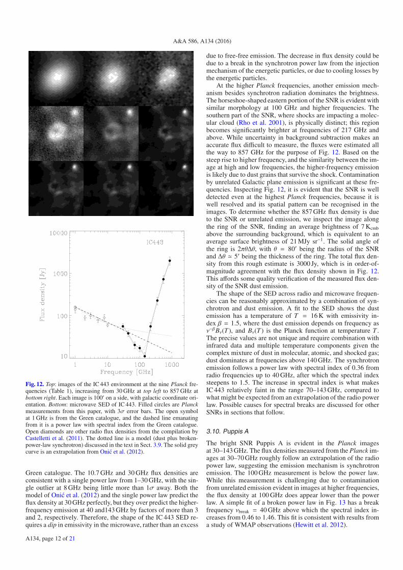
Fig. 12. Top: images of the IC 443 environment at the nine Planck fre-quencies (Table 1), increasing from 30 GHz at top left to 857 GHz atbottom right. Each image is 100′ on a side, with galactic coordinate ori-entation. Bottom: microwave SED of IC 443. Filled circles are Planckmeasurements from this paper, with 3σ error bars. The open symbolat 1 GHz is from the Green catalogue, and the dashed line emanatingfrom it is a power law with spectral index from the Green catalogue.Open diamonds are other radio flux densities from the compilation byCastelletti et al. (2011). The dotted line is a model (dust plus broken-power-law synchrotron) discussed in the text in Sect. 3.9. The solid greycurve is an extrapolation from Onic et al. (2012).

Green catalogue. The 10.7 GHz and 30 GHz flux densities areconsistent with a single power law from 1–30 GHz, with the sin-gle outlier at 8 GHz being little more than 1σ away. Both themodel of Onic et al. (2012) and the single power law predict theflux density at 30 GHz perfectly, but they over predict the higher-frequency emission at 40 and143 GHz by factors of more than 3and 2, respectively. Therefore, the shape of the IC 443 SED re-quires a dip in emissivity in the microwave, rather than an excess

due to free-free emission. The decrease in flux density could bedue to a break in the synchrotron power law from the injectionmechanism of the energetic particles, or due to cooling losses bythe energetic particles.

At the higher Planck frequencies, another emission mech-anism besides synchrotron radiation dominates the brightness.The horseshoe-shaped eastern portion of the SNR is evident withsimilar morphology at 100 GHz and higher frequencies. Thesouthern part of the SNR, where shocks are impacting a molec-ular cloud (Rho et al. 2001), is physically distinct; this regionbecomes significantly brighter at frequencies of 217 GHz andabove. While uncertainty in background subtraction makes anaccurate flux difficult to measure, the fluxes were estimated allthe way to 857 GHz for the purpose of Fig. 12. Based on thesteep rise to higher frequency, and the similarity between the im-age at high and low frequencies, the higher-frequency emissionis likely due to dust grains that survive the shock. Contaminationby unrelated Galactic plane emission is significant at these fre-quencies. Inspecting Fig. 12, it is evident that the SNR is welldetected even at the highest Planck frequencies, because it iswell resolved and its spatial pattern can be recognised in theimages. To determine whether the 857 GHz flux density is dueto the SNR or unrelated emission, we inspect the image alongthe ring of the SNR, finding an average brightness of 7 Kcmbabove the surrounding background, which is equivalent to anaverage surface brightness of 21 MJy sr−1. The solid angle ofthe ring is 2πθΔθ, with θ = 80′ being the radius of the SNRand Δθ � 5′ being the thickness of the ring. The total flux den-sity from this rough estimate is 3000 Jy, which is in order-of-magnitude agreement with the flux density shown in Fig. 12.This affords some quality verification of the measured flux den-sity of the SNR dust emission.

The shape of the SED across radio and microwave frequen-cies can be reasonably approximated by a combination of syn-chrotron and dust emission. A fit to the SED shows the dustemission has a temperature of T = 16 K with emissivity in-dex β = 1.5, where the dust emission depends on frequency asν−βBν(T ), and Bν(T ) is the Planck function at temperature T .The precise values are not unique and require combination withinfrared data and multiple temperature components given thecomplex mixture of dust in molecular, atomic, and shocked gas;dust dominates at frequencies above 140 GHz. The synchrotronemission follows a power law with spectral index of 0.36 fromradio frequencies up to 40 GHz, after which the spectral indexsteepens to 1.5. The increase in spectral index is what makesIC 443 relatively faint in the range 70–143 GHz, compared towhat might be expected from an extrapolation of the radio powerlaw. Possible causes for spectral breaks are discussed for otherSNRs in sections that follow.

3.10. Puppis A

The bright SNR Puppis A is evident in the Planck imagesat 30–143 GHz. The flux densities measured from the Planck im-ages at 30–70 GHz roughly follow an extrapolation of the radiopower law, suggesting the emission mechanism is synchrotronemission. The 100 GHz measurement is below the power law.While this measurement is challenging due to contaminationfrom unrelated emission evident in images at higher frequencies,the flux density at 100 GHz does appear lower than the powerlaw. A simple fit of a broken power law in Fig. 13 has a breakfrequency νbreak = 40 GHz above which the spectral index in-creases from 0.46 to 1.46. This fit is consistent with results froma study of WMAP observations (Hewitt et al. 2012).

A134, page 12 of 21

Planck Collaboration: Planck supernova remnant survey

Fig. 13. Top: images of the Puppis A environment at the nine Planckfrequencies (Table 1), increasing from 30 GHz at top left to 857 GHz atbottom right. Each image is 100′ on a side, with galactic coordinate ori-entation. Bottom: microwave SED of Puppis A. Filled circles are Planckmeasurements from this paper, with 3σ error bars. The open symbolat 1 GHz is from the Green catalogue, and the dashed line emanatingfrom it is a power law with spectral index from the Green catalogue.Open diamonds are radio flux densities from the Milne et al. (1993) andWMAP fluxes from Hewitt et al. (2012).

3.11. Vela

The very large Vela SNR is prominent in the lowest-frequencyPlanck images; Fig. 14 shows a well-resolved shell evenat 30 GHz. The centre of the image is shifted (by 1◦ upwardin galactic latitude) from the Green catalogue position, so as toinclude the entire SNR shell. The object at the right-hand edgeof the lower-frequency panels of Fig. 14 is actually the previousSNR from the survey, Puppis A.

Fig. 14. Top: images of the Vela environment at the nine Planck fre-quencies (Table 1), increasing from 30 GHz at top left to 857 GHz atbottom right. Each image is 400′ on a side, with galactic coordinate ori-entation, centred 1◦ north of Vela-X. Bottom: microwave SED of Vela.Filled circles are Planck measurements from this paper, with 3σ er-ror bars. The open symbol at 1 GHz is from the Green catalogue, andthe dashed line emanating from it is a power law with spectral indexfrom the Green catalogue. Downward arrows show the Planck high-frequency flux density measurements that are contaminated by unre-lated foreground emission.

At frequencies above 70 GHz, the SNR is confused withunrelated emission from cold molecular clouds and cold cores.However, some synchrotron features remain visible at higherfrequencies. The relatively bright feature near the lower centreof the image is Vela-X, the bright nest part of the radio SNR.This feature can be traced all the way to 353 GHz, with contrast

A134, page 13 of 21

A&A 586, A134 (2016)

steadily decreasing at higher and higher frequencies. Some dust-dominated features are visible at low frequencies. The brightfeature at the centre-top of the low-frequency panels of Fig. 14overlap with the very prominent set of knots and filaments inthe high-frequency images, with a steadily decreasing bright-ness for the knots and filaments. At frequencies above 100 GHz,the dust features dominate here, while at 30–70 GHz the syn-chrotron from the SNR dominates.

The 30–70 GHz Planck flux densities follow an extrapola-tion of the radio power law with slightly higher spectral index,indicating the microwave emission mechanism is synchrotron,with no evidence for a spectral break.

3.12. PKS 1209-51/52

The barrel-shaped (Kesteven & Caswell 1987) SNR PKS1209-51/52 is detected by Planck at low frequencies. The angularstructure of the SNR overlaps in spatial scales with the CMB,so PKS1209-51/52 was masked in the CMB maps. Therefore,Fig. 15 shows the total intensity for this SNR, rather than theCMB-subtracted intensity. At 30–70 GHz, the SNR is clearlyevident because it is significantly brighter than the CMB andhas the location and size seen in lower-frequency radio im-ages. At 100–217 GHz, the SNR is lost in CMB fluctuations.At 353–857 GHz, the region is dominated by interstellar dustemission. The object near the centre of the SNR in the high-frequency images is a reflection nebula, identified by Brand et al.(1986, object 381) on optical places as a 3′ possible reflectionnebula; it was also noted as a far-infrared source without corre-sponding strong H I emission (Reach et al. 1993, object 9095).There is no evidence for this object to be associated with theSNR nor the neutron star suspected to be the remnant of the pro-genitor (Vasisht et al. 1997, X-ray source 1E 1207.4-5209), lo-cated 12′ away. It is nonetheless remarkable that the source isright at the centre of the SNR.

Figure 15 shows the low-frequency emission seen by Planckcontinues the radio synchrotron spectrum closely up to 70 GHz,with no evidence for a spectral break.

3.13. RCW 86

The RCW 86 supernova remnant, possibly that of a Type I SNwithin a stellar wind bubble (Williams et al. 2011), is evidentin the low-frequency 30–70 GHz Planck images. At higher fre-quencies the synchrotron emission from the SNR is confusedwith other emission. The feature near the left-centre of the high-est 6 frequency images of RCW 86 in Fig. 16 is a dark molecularcloud, DB 315.7-2.4 (Dutra & Bica 2002). The Planck emissionfrom this location is due to dust, with brightness steadily increas-ing with frequency over the Planck domain. The cloud is locatednear the edge of the SNR, and the CO velocity (–37 km s−1;Otrupcek et al. 2000) is approximately as expected for a cloudat the distance estimate for the SNR (2.3 kpc). Any relationbetween the cold molecular cloud and the SNR is only plau-sible; there is no direct evidence for interaction. In any event,the dust in this cloud makes it impossible to measure the syn-chrotron brightness at 100 GHz, and the 70 GHz flux has higheruncertainty.

For the SNR synchrotron emission, the Planck flux densities,shown in Fig. 16, are consistent within 1σ with an extrapola-tion of the radio synchrotron power law. The existence of X-raysynchrotron emission (Rho et al. 2002) suggests that the energydistribution of relativistic electrons continues to high energy.

Fig. 15. Top: images of the PKS 1209-51/52 environment at the ninePlanck frequencies (Table 1), increasing from 30 GHz at top leftto 857 GHz at bottom right. Each image is 180′ on a side, with galac-tic coordinate orientation. Bottom: microwave SED of PKS 1209-52.Filled circles are Planck measurements from this paper, with 3σ er-ror bars. The open symbol at 1 GHz is from the Green catalogue, andthe dashed line emanating from it is a power law with spectral indexfrom the Green catalogue. Open diamonds are radio flux densities fromMilne & Haynes (1994). The downward arrow shows a Planck high-frequency flux density measurement that was contaminated by unre-lated foreground emission.

3.14. MSH 15-56

The radio-bright SNR MSH 15-56 is well detected in the firstfive Planck frequencies, 30–143 GHz. The SNR is a “compos-ite”, with a steep-spectrum shell and a brighter, flat-spectrumplerionic core. The Planck flux densities do not follow a sin-gle power law matching the published radio flux densities. Just

A134, page 14 of 21

Planck Collaboration: Planck supernova remnant survey

Fig. 16. Top: images of the RCW 86 environment at the nine Planckfrequencies (Table 1), increasing from 30 GHz at top left to 857 GHz atbottom right. Each image is 100′ on a side, with galactic coordinate ori-entation. Bottom: microwave SED of RCW 86. Filled circles are Planckmeasurements from this paper, with 3σ error bars. The open symbolat 1 GHz is from the Green catalogue, and the dashed line emanatingfrom it is a power law with spectral index from the Green catalogue. Theopen diamonds is the 5 GHz flux density from Caswell et al. (1975).

connecting the 1 GHz radio flux densities to the Planck flux den-sities, the spectral index is in the range 0.3–0.5. The Planck fluxdensities themselves follow a steeper power law than can matchthe radio flux densities, and suggest a break in the spectral in-dex. Figure 17 shows a broken-power-law fit, where the spectralindex steepens from 0.31 to 0.9 at 30 GHz. Low-frequency radioobservations show that the plerionic core of the SNR has a flatterspectral index than the shell, while higher-frequency flux densi-ties of the core alone from 4.8 to 8.6 GHz have a spectral index

Fig. 17. Top: images of the MSH 15-56 environment at the nine Planckfrequencies (Table 1), increasing from 30 GHz at top left to 857 GHzat bottom right. Each image is 100′ on a side, with galactic coordinateorientation. Bottom: microwave SED of MSH 15-56. Filled circles arePlanck measurements from this paper, with 3σ error bars. The opensymbol at 1 GHz is from the Green catalogue, and the dashed line em-anating from it is a power law with spectral index from the Green cat-alogue. Open diamonds are radio flux densities from the Dickel et al.(2000) and Milne et al. (1979) that constrain the slope through thePlanck data.

of 0.85 (Dickel et al. 2000). The relatively flat spectral index atradio frequencies and up to about 30 GHz may indicate injectionof fresh electrons, as in the Crab and 3C 58, which are driven bypulsar wind nebulae. However, there has been, to date, no pulsardetected in MSH 15-56, and the spectral index is not as flat asin the known, young pulsar wind nebulae. The apparent break inspectral index to a stepper slope above 30 GHz suggests possibleenergy loss of the highest-energy particles.

A134, page 15 of 21

A&A 586, A134 (2016)

Fig. 18. Top: images of the SN 1006 environment at the nine Planckfrequencies (Table 1), increasing from 30 GHz at top left to 857 GHz atbottom right. Each image is 100′ on a side, with galactic coordinate ori-entation. Bottom: microwave SED of SN 1006. Filled circles are Planckmeasurements from this paper, with 3σ error bars. The open symbolat 1 GHz is from the Green catalogue, and the dashed line emanatingfrom it is a power law with spectral index from the Green catalogue.The dotted line is a broken power-law fit discussed in the text.

3.15. SN 1006

SN 1006 is well-detected at 30–44 GHz. At higher frequenciesit becomes faint and possibly confused with unrelated emission.However, the field is not as crowded as it is for most other SNRs,and we suspect that the observed decrement in flux density be-low the extrapolation of the radio power law at 70 and 100 GHzmay be due to a real break in the spectral index. If so, then thefrequency of that break is in the range 20 < νbreak < 30 GHz. Forillustration, Fig. 18 shows a broken power-law fit with νbreak =22 GHz, above which the spectral index steepens from α = 0.5to α = 1 as predicted for synchrotron losses. The Planck dataappear to match this model well.

Table 5. Sychrotron spectral indices.

Spectral index νbreak

SNR . . . . . . α1 α2 [GHz]

G21.5-0.9 . . . 0.05 0.55 45W 44 . . . . . . 0.37 1.37 45CTB 80 . . . . 0.80 ... noneHB 21 . . . . . 0.38 0.88 33C 58 . . . . . 0.07 0.57 25IC 443 . . . . . 0.36 1.56 40Puppis A . . . 0.46 1.46 40MSH 15-56 . . 0.31 0.9 30SN 1006 . . . 0.50 1.0 22

4. Conclusions

The flux densities of 16 known Galactic supernova remnantswere measured from the Planck microwave all-sky survey withthe following conclusions. We find new evidence for spectral in-dex breaks in G21.5-0.9, HB 21, MSH 15-56, SN 1006, and weconfirm the previously detected spectral break in 3C 58, includ-ing a new detection with Herschel.

Table 5 summarizes the new spectral indices required to fitthe radio through microwave SED of SNRs. These values corre-spond to the dashed lines in the SEDs for each SNR in this paper.For each SNR in this paper for which the Planck data indicatedin a spectrum noticeably different from the radio power-law ex-trapolation, the frequency of the spectral break (νbreak) and thespectral index at lower and higher frequencies (α1 and α2, re-spectively) are listed. The actual SEDs should be consulted be-fore using the spectral index values by themselves, because theyare only applicable over the region shown, and they are onlymathematical approximations to what is more likely a continu-ous distribution of energies with evolving losses.

The breaks in spectral index are consistent with synchrotronlosses of electrons injected by a central source. We extend the ra-dio synchrotron spectrum for young SNRs Cas A and Tycho withno evidence for extra emission mechanisms. The distinction inproperties between those supernova remnants that do or do notshow a break in their power-law spectral index is not readily ev-ident. The supernova remnants with spectral breaks include ex-amples that range from bright to faint and young to mature, andthey also include examples both with and without stellar rem-nants. A combination of cosmic-ray acceleration by the shocksand the pulsars, deceleration in denser environments, and ageingmay lead to the variation in synchrotron shapes.

Acknowledgements. The Planck Collaboration acknowledges the support of:ESA; CNES, and CNRS/INSU-IN2P3-INP (France); ASI, CNR, and INAF(Italy); NASA and DoE (USA); STFC and UKSA (UK); CSIC, MINECO,JA and RES (Spain); Tekes, AoF, and CSC (Finland); DLR and MPG(Germany); CSA (Canada); DTU Space (Denmark); SER/SSO (Switzerland);RCN (Norway); SFI (Ireland); FCT/MCTES (Portugal); ERC and PRACE (EU).A description of the Planck Collaboration and a list of its members, indicatingwhich technical or scientific activities they have been involved in, can be foundat http://www.cosmos.esa.int/web/planck/planck-collaboration.

ReferencesAMI Consortium, Perrott, Y. C., Green, D. A., et al. 2012, MNRAS, 421, L6Arendt, R. G., Dwek, E., & Leisawitz, D. 1992, ApJ, 400, 562Ashworth, Jr., W. B. 1980, Journal for the History of Astronomy, 11, 1Aumann, H. H., Fowler, J. W., & Melnyk, M. 1990, AJ, 99, 1674Baars, J. W. M., Genzel, R., Pauliny-Toth, I. I. K., & Witzel, A. 1977, A&A, 61,

99Barlow, M. J., Krause, O., Swinyard, B. M., et al. 2010, A&A, 518, L138Bersanelli, M., Mandolesi, N., Butler, R. C., et al. 2010, A&A, 520, A4Bietenholz, M. F., & Bartel, N. 2008, MNRAS, 386, 1411Brand, J., Blitz, L., & Wouterloot, J. G. A. 1986, A&AS, 65, 537

A134, page 16 of 21

Planck Collaboration: Planck supernova remnant survey

Camilo, F., Ransom, S. M., Gaensler, B. M., et al. 2006, ApJ, 637, 456Castelletti, G., Dubner, G., Golap, K., et al. 2003, AJ, 126, 2114Castelletti, G., Dubner, G., Clarke, T., & Kassim, N. E. 2011, A&A, 534, A21Caswell, J. L., Clark, D. H., & Crawford, D. F. 1975, Austr. J. Phys. Astrophys.

Suppl., 37, 39Dickel, J. R., Milne, D. K., & Strom, R. G. 2000, ApJ, 543, 840Dutra, C. M., & Bica, E. 2002, A&A, 383, 631Gao, X. Y., Han, J. L., Reich, W., et al. 2011, A&A, 529, A159Gomez, H. L., Clark, C. J. R., Nozawa, T., et al. 2012, MNRAS, 420, 3557Górski, K. M., Hivon, E., Banday, A. J., et al. 2005, ApJ, 622, 759Green, D. A. 1986, MNRAS, 218, 533Green, D. A. 2009, BASI, 37, 45 (Green catalogue)Green, D. A., & Scheuer, P. A. G. 1992, MNRAS, 258, 833Green, A. J., Baker, J. R., & Landecker, T. L. 1975, A&A, 44, 187Gupta, Y., Mitra, D., Green, D. A., & Acharyya, A. 2005, Curr. Sci., 89, 853Han, J. L., Reich, W., Sun, X. H., et al. 2013, Inter. J. Mod. Phys. Conf. Ser., 23,

82Hewitt, J. W., Grondin, M.-H., Lemoine-Goumard, M., et al. 2012, ApJ, 759, 89Kesteven, M. J., & Caswell, J. L. 1987, A&A, 183, 118Klein, U., Emerson, D. T., Haslam, C. G. T., & Salter, C. J. 1979, A&A, 76, 120Kothes, R., Fedotov, K., Foster, T. J., & Uyanıker, B. 2006, A&A, 457, 1081Kundu, M. R., & Velusamy, T. 1972, A&A, 20, 237Lamarre, J., Puget, J., Ade, P. A. R., et al. 2010, A&A, 520, A9Macías-Pérez, J. F., Mayet, F., Aumont, J., & Désert, F.-X. 2010, ApJ, 711, 417Mandolesi, N., Bersanelli, M., Butler, R. C., et al. 2010, A&A, 520, A3Mantovani, F., Reich, W., Salter, C. J., & Tomasi, P. 1985, A&A, 145, 50Mason, B. S., Leitch, E. M., Myers, S. T., Cartwright, J. K., & Readhead, A. C. S.

1999, AJ, 118, 2908McCray, R., & Wang, Z., eds. 1996, Supernovae and Supernova Remnants: IAU

Coll. 145 (Cambridge University Press)Mennella, A., Butler, R. C., Curto, A., et al. 2011, A&A, 536, A3Milne, D. K., & Haynes, R. F. 1994, MNRAS, 270, 106Milne, D. K., Goss, W. M., Haynes, R. F., et al. 1979, MNRAS, 188, 437Milne, D. K., Stewart, R. T., & Haynes, R. F. 1993, MNRAS, 261, 366Morsi, H. W., & Reich, W. 1987, A&AS, 69, 533Onic, D., Uroševic, D., Arbutina, B., & Leahy, D. 2012, ApJ, 756, 61Otrupcek, R. E., Hartley, M., & Wang, J.-S. 2000, PASA, 17, 92Pivato, G., Hewitt, J. W., Tibaldo, L., et al. 2013, ApJ, 779, 179Planck Collaboration I. 2011, A&A, 536, A1Planck Collaboration II. 2011, A&A, 536, A2Planck Collaboration VII. 2011, A&A, 536, A7 (ERCSC)Planck Collaboration IV. 2014, A&A, 571, A4Planck Collaboration V. 2014, A&A, 571, A5Planck Collaboration VII. 2014, A&A, 571, A7Planck Collaboration VIII. 2014, A&A, 571, A8Planck Collaboration XII. 2014, A&A, 571, A12Planck HFI Core Team 2011a, A&A, 536, A4Planck HFI Core Team 2011b, A&A, 536, A6Reach, W. T., Heiles, C., & Koo, B.-C. 1993, ApJ, 412, 127Reich, W., Zhang, X., & Fürst, E. 2003, A&A, 408, 961Reynolds, S. P. 2009, ApJ, 703, 662Reynolds, S. P. 2011, Ap&SS, 336, 257Rho, J., Jarrett, T. H., Cutri, R. M., & Reach, W. T. 2001, ApJ, 547, 885Rho, J., Dyer, K. K., Borkowski, K. J., & Reynolds, S. P. 2002, ApJ, 581, 1116Salter, C. J., Reynolds, S. P., Hogg, D. E., Payne, J. M., & Rhodes, P. J. 1989,

ApJ, 338, 171Scaife, A., Green, D. A., Battye, R. A., et al. 2007, MNRAS, 377, L69Slane, P., Helfand, D. J., Reynolds, S. P., et al. 2008, ApJ, 676, L33Sofue, Y., Takahara, F., Hirabayashi, H., Inoue, M., & Nakai, N. 1983, PASJ, 35,

437Sun, X. H., Reich, W., Han, J. L., Reich, P., & Wielebinski, R. 2006, A&A, 447,

937Sun, X. H., Reich, P., Reich, W., et al. 2011, A&A, 536, A83Tauber, J. A., Mandolesi, N., Puget, J., et al. 2010, A&A, 520, A1Uyanıker, B., Reich, W., Yar, A., & Fürst, E. 2004, A&A, 426, 909Vasisht, G., Kulkarni, S. R., Anderson, S. B., Hamilton, T. T., & Kawai, N. 1997,

ApJ, 476, L43Velusamy, T., Kundu, M. R., & Becker, R. H. 1976, A&A, 51, 21Weiland, J. L., Odegard, N., Hill, R. S., et al. 2011, ApJS, 192, 19Williams, B. J., Blair, W. P., Blondin, J. M., et al. 2011, ApJ, 741, 96Willis, A. G. 1973, A&A, 26, 237Zacchei, A., Maino, D., Baccigalupi, C., et al. 2011, A&A, 536, A5

1 APC, AstroParticule et Cosmologie, Université Paris Diderot,CNRS/IN2P3, CEA/lrfu, Observatoire de Paris, Sorbonne ParisCité, 10, rue Alice Domon et Léonie Duquet, 75205 Paris Cedex 13,France

2 Aalto University Metsähovi Radio Observatory and Dept of RadioScience and Engineering, PO Box 13000, 00076 AALTO, Finland

3 African Institute for Mathematical Sciences, 6–8 Melrose Road,Muizenberg, 7945 Cape Town, South Africa

4 Agenzia Spaziale Italiana Science Data Center, via del Politecnicosnc, 00133 Roma, Italy

5 Astrophysics Group, Cavendish Laboratory, University ofCambridge, J J Thomson Avenue, Cambridge CB3 0HE, UK

6 Astrophysics & Cosmology Research Unit, School of Mathematics,Statistics & Computer Science, University of KwaZulu-Natal,Westville Campus, Private Bag X54001, 4000 Durban, South Africa

7 Atacama Large Millimeter/submillimeter Array, ALMA SantiagoCentral Offices, Alonso de Cordova 3107, Vitacura, Casilla763 0355, Santiago, Chile

8 CGEE, SCS Qd 9, Lote C, Torre C, 4◦ andar, Ed. Parque CidadeCorporate, CEP 70308-200, Brasília, DF,Ê Brazil

9 CITA, University of Toronto, 60 St. George St., Toronto, ON M5S3H8, Canada

10 CNRS, IRAP, 9 Av. colonel Roche, BP 44346, 31028 ToulouseCedex 4, France

11 California Institute of Technology, Pasadena, CA 91101 California,USA

12 Centro de Estudios de Física del Cosmos de Aragón (CEFCA),Plaza San Juan, 1, planta 2, 44001 Teruel, Spain

13 Computational Cosmology Center, Lawrence Berkeley NationalLaboratory, Berkeley, CA 91101 California, USA

14 DSM/Irfu/SPP, CEA-Saclay, 91191 Gif-sur-Yvette Cedex, France15 DTU Space, National Space Institute, Technical University of

Denmark, Elektrovej 327, 2800 Kgs. Lyngby, Denmark16 Département de Physique Théorique, Université de Genève, 24,

Quai E. Ansermet, 1211 Genève 4, Switzerland17 Departamento de Física Fundamental, Facultad de Ciencias,

Universidad de Salamanca, 37008 Salamanca, Spain18 Departamento de Física, Universidad de Oviedo, Avda. Calvo Sotelo

s/n, 33003 Oviedo, Spain19 Department of Astrophysics/IMAPP, Radboud University

Nijmegen, PO Box 9010, 6500 GL Nijmegen, The Netherlands20 Department of Physics & Astronomy, University of British

Columbia, 6224 Agricultural Road, Vancouver, British Columbia,Canada

21 Department of Physics and Astronomy, Dana and David DornsifeCollege of Letter, Arts and Sciences, University of SouthernCalifornia, Los Angeles, CA 90089, USA

22 Department of Physics and Astronomy, University College London,London WC1E 6BT, UK

23 Department of Physics, Florida State University, Keen PhysicsBuilding, 77 Chieftan Way, Tallahassee, Florida, USA

24 Department of Physics, Gustaf Hällströmin katu 2a, University ofHelsinki, 00100 Helsinki, Finland

25 Department of Physics, Princeton University, Princeton, NJ 08544New Jersey, USA

26 Department of Physics, University of California, Santa Barbara,CA 94612 California, USA

27 Dipartimento di Fisica e Astronomia G. Galilei, Università degliStudi di Padova, via Marzolo 8, 35131 Padova, Italy

28 Dipartimento di Fisica e Scienze della Terra, Università di Ferrara,via Saragat 1, 44122 Ferrara, Italy

29 Dipartimento di Fisica, Università La Sapienza, P. le A. Moro 2,00185 Roma, Italy

30 Dipartimento di Fisica, Università degli Studi di Milano, via Celoria,16 Milano, Italy

31 Dipartimento di Fisica, Università degli Studi di Trieste, via A.Valerio 2, 34128 Trieste, Italy

32 Dipartimento di Fisica, Università di Roma Tor Vergata, via dellaRicerca Scientifica, 1 Roma, Italy

33 Discovery Center, Niels Bohr Institute, Blegdamsvej 17, 2100Copenhagen, Denmark

34 Discovery Center, Niels Bohr Institute, Copenhagen University,Blegdamsvej 17, 2100 Copenhagen, Denmark

A134, page 17 of 21

A&A 586, A134 (2016)

35 European Southern Observatory, ESO Vitacura, Alonso de Cordova3107, Vitacura, Casilla 19001, Santiago, Chile

36 European Space Agency, ESAC, Planck Science Office, Caminobajo del Castillo, s/n, Urbanización Villafranca del Castillo,Villanueva de la Cañada, 28692 Madrid, Spain

37 European Space Agency, ESTEC, Keplerlaan 1, 2201 AZNoordwijk, The Netherlands

38 Facoltà di Ingegneria, Università degli Studi e-Campus, viaIsimbardi 10, 22060 Novedrate (CO), Italy

39 Gran Sasso Science Institute, INFN, viale F. Crispi 7, 67100L’Aquila, Italy

40 Helsinki Institute of Physics, Gustaf Hällströmin katu 2, Universityof Helsinki, 00100 Helsinki, Finland

41 INAF–Osservatorio Astrofisico di Catania, via S. Sofia 78, Catania,Italy

42 INAF–Osservatorio Astronomico di Padova, Vicolodell’Osservatorio 5, Padova, Italy

43 INAF–Osservatorio Astronomico di Roma, via di Frascati 33,Monte Porzio Catone, Italy

44 INAF–Osservatorio Astronomico di Trieste, via G.B. Tiepolo 11,Trieste, Italy

45 INAF/IASF Bologna, via Gobetti 101, 40126 Bologna, Italy46 INAF/IASF Milano, via E. Bassini 15, 20100 Milano, Italy47 INFN, Sezione di Bologna, via Irnerio 46, 40126 Bologna, Italy48 INFN, Sezione di Roma 1, Università di Roma Sapienza, Piazzale

Aldo Moro 2, 00185 Roma, Italy49 INFN/National Institute for Nuclear Physics, via Valerio 2, 34127

Trieste, Italy50 IPAG: Institut de Planétologie et d’Astrophysique de Grenoble,

Université Grenoble Alpes, IPAG, 38000 Grenoble, France51 CNRS, IPAG, 38000 Grenoble, France52 Imperial College London, Astrophysics group, Blackett Laboratory,

Prince Consort Road, London, SW7 2AZ, UK53 Infrared Processing and Analysis Center, California Institute of

Technology, Pasadena, CA 91125, USA54 Institut d’Astrophysique Spatiale, CNRS (UMR 8617) Université

Paris-Sud 11, Bâtiment 121, 91440 Orsay, France55 Institut d’Astrophysique de Paris, CNRS (UMR 7095), 98 bis

Boulevard Arago, 75014 Paris, France56 Institute for Space Sciences, 077125 Bucharest-Magurale, Romania57 Institute of Astronomy, University of Cambridge, Madingley Road,

Cambridge CB3 0HA, UK58 Institute of Theoretical Astrophysics, University of Oslo, Blindern,

0371 Oslo, Norway59 Instituto de Física de Cantabria (CSIC-Universidad de Cantabria),

Avda. de los Castros s/n, 39005 Santander, Spain60 Istituto Nazionale di Fisica Nucleare, Sezione di Padova, via

Marzolo 8, 35131 Padova, Italy61 Jet Propulsion Laboratory, California Institute of Technology, 4800

Oak Grove Drive, Pasadena, California, USA62 Jodrell Bank Centre for Astrophysics, Alan Turing Building, School

of Physics and Astronomy, The University of Manchester, OxfordRoad, Manchester, M13 9PL, UK

63 Kavli Institute for Cosmology Cambridge, Madingley Road,Cambridge, CB3 0HA, UK

64 Kazan Federal University, 18 Kremlyovskaya St., 420008 Kazan,Russia

65 LAL, Université Paris-Sud, CNRS/IN2P3, 91400 Orsay, France

66 LERMA, CNRS, Observatoire de Paris, 61 Avenue del’Observatoire, 75014 Paris, France

67 Laboratoire AIM, IRFU/Service d’Astrophysique – CEA/DSM –CNRS – Université Paris Diderot, Bât. 709, CEA-Saclay, 91191 Gif-sur-Yvette Cedex, France

68 Laboratoire Traitement et Communication de l’Information, CNRS(UMR 5141) and Télécom ParisTech, 46 rue Barrault, 75634 ParisCedex 13, France

69 Laboratoire de Physique Subatomique et Cosmologie, UniversitéGrenoble-Alpes, CNRS/IN2P3, 53 rue des Martyrs, 38026 GrenobleCedex, France

70 Laboratoire de Physique Théorique, Université Paris-Sud 11 &CNRS, Bâtiment 210, 91405 Orsay, France

71 Lawrence Berkeley National Laboratory, Berkeley, CA 94720California, USA

72 Lebedev Physical Institute of the Russian Academy of Sciences,Astro Space Centre, 84/32 Profsoyuznaya st., GSP-7, 117997Moscow, Russia

73 Max-Planck-Institut für Astrophysik, Karl-Schwarzschild-Str. 1,85741 Garching, Germany

74 Max-Planck-Institut für Radioastronomie, Auf dem Hügel 69,53121 Bonn, Germany

75 National Radio Astronomy Observatory, 520 Edgemont Road,Charlottesville VA 22903-2475, USA

76 National University of Ireland, Department of ExperimentalPhysics, Maynooth, Co. Kildare, Ireland

77 Nicolaus Copernicus Astronomical Center, Bartycka 18, 00-716Warsaw, Poland

78 Niels Bohr Institute, Blegdamsvej 17, 2100 Copenhagen, Denmark79 Niels Bohr Institute, Copenhagen University, Blegdamsvej 17, 2100

Copenhagen, Denmark80 Optical Science Laboratory, University College London, Gower

Street, London, UK81 SETI Institute and SOFIA Science Center, NASA Ames Research

Center, MS 211-3, Mountain View, CA 94035, USA82 SISSA, Astrophysics Sector, via Bonomea 265, 34136, Trieste, Italy83 School of Physics and Astronomy, Cardiff University, Queens

Buildings, The Parade, Cardiff, CF24 3AA, UK84 Sorbonne Université-UPMC, UMR 7095, Institut d’Astrophysique

de Paris, 98 bis Boulevard Arago, 75014 Paris, France85 Space Sciences Laboratory, University of California, Berkeley,

CA 94720 California, USA86 Special Astrophysical Observatory, Russian Academy of Sciences,

Nizhnij Arkhyz, Zelenchukskiy region, Karachai-CherkessianRepublic, 369167, Russia

87 UPMC Univ Paris 06, UMR 7095, 98 bis Boulevard Arago, 75014Paris, France

88 Université de Toulouse, UPS-OMP, IRAP, 31028 Toulouse Cedex 4,France

89 Universities Space Research Association, Stratospheric Observatoryfor Infrared Astronomy, MS 232-11, Moffett Field, CA 94035, USA

90 University of Granada, Departamento de Física Teórica y delCosmos, Facultad de Ciencias, 18010 Granada, Spain

91 University of Granada, Instituto Carlos I de Física Teórica yComputacional, 18010 Granada, Spain

92 Warsaw University Observatory, Aleje Ujazdowskie 4, 00-478Warszawa, Poland

A134, page 18 of 21

Planck Collaboration: Planck supernova remnant survey

Appendix A: Aperture photometry details

More details on the aperture photometry are provided inTable A.1. For each flux density measurement, the followingquantities are listed.

1 The supernova remnant (SNR) name, in the same order as inTables 2 and 3.

2 The observing frequency in GHz.3 “Flux” is the aperture-corrected, background-subtracted flux

of the source with its uncertainty. The uncertainty is a quadra-ture combination of the statistical uncertainty and the flux cal-ibration uncertainty. The flux calibration uncertainty is theflux multiplied by the mission calibration uncertainty fromTable 1. The statistical uncertainty is the rms of the pixel val-ues in the background annulus, Irms, multiplied by the numberof pixels in the on-source aperture and divided by the square-root of the number of pixels in the off-source annulus, thenscaled by the same aperture correction as was applied to theflux.

4 θap is the aperture radius, within which the source flux wassummed.

5 fA is the aperture correction factor, from Eq. (2).6 Fbg is the flux of the background that was subtracted from

the on-source sum of the source flux. This was calculated bytaking the median brightness within the background annulus,then multiplying by the area of the on-source aperture. To aiddirect comparison we also applied the same aperture correc-tion as was applied to the source flux. Because of the longlines of sight through the Galactic disk at the locations ofmost of the SNRs, the backgrounds are high, and Fbg is oftenhigher than the flux of the SNR. In itself, this is not a funda-mental limitation, because a smooth background can be muchbrighter than the target without affecting the photometry.

7 Ipeak is the peak intensity in the on-source aperture, in the unitsof the map for which the photometry was being performed.For frequencies 30–353 GHz, the units are mK in thermody-namic CBM brightness temperature units. For 545–857 GHz,the units are MJy sr−1.

8 Ibg is the median intensity in the background annulus, in thesame units units as Ipeak.

9 Irms is the standard deviation (rms) of the pixel values in thebackground annulus, in the same units as Ipeak. The peak,per-pixel signal-to-noise for each target can be estimated asIpeak/Irms because the target causes the brightest pixel in theon-source aperture. This gives a quantitative measure of howreadily visible the target is, at the angular scale of the Planckbeam.

A134, page 19 of 21

A&A 586, A134 (2016)

Table A.1. Aperture photometry details for Planck flux density measurements of supernova remnants.

(1) (2) (3) (4) (5) (6) (7) (8) (9)Source Freq. Flux θap fA Fbg Ipeak Ibg Irms

[GHz] [Jy] [′] [Jy] a a a

G21.5-0.9 70 4.3 ± 0.6 10.2 1.4 7.1 3.1 1.4 0.4G21.5-0.9 100 2.5 ± 0.5 8.1 1.4 17.6 4.5 3.1 0.5G21.5-0.9 143 2.9 ± 0.4 6.0 1.4 15.4 4.5 2.9 0.3W44 30 121.0 ± 8.2 36.1 1.4 149.2 28.6 11.6 5.8W44 44 67.2 ± 5.2 33.2 1.4 103.1 11.0 4.5 2.2W44 70 29.5 ± 3.3 28.0 1.0 64.1 5.3 2.3 1.6CTB80 30 14.5 ± 1.7 64.9 1.0 39.3 3.3 1.3 2.2CTB80 44 8.4 ± 1.2 63.3 1.0 25.8 1.3 0.4 1.0CygLoop 30 22.2 ± 1.6 174.3 1.0 61.1 1.3 0.3 0.4HB21 30 15.4 ± 1.7 93.3 1.0 110.6 3.6 1.8 0.8HB21 44 10.0 ± 1.2 92.2 1.0 74.8 1.3 0.6 0.3CasA 30 227.2 ± 11.4 25.0 1.4 15.8 76.8 2.6 1.5CasA 44 139.7 ± 7.0 20.6 1.4 12.1 33.6 1.4 0.7CasA 70 108.9 ± 5.5 10.4 1.4 4.4 40.8 0.8 0.7CasA 100 93.9 ± 4.7 8.4 1.4 5.7 34.5 0.9 0.3CasA 143 72.7 ± 3.7 6.5 1.4 7.2 28.7 1.2 0.3CasA 217 62.2 ± 3.2 5.1 1.4 21.4 34.1 4.3 0.6CasA 353 59.9 ± 3.9 5.0 1.4 82.5 72.8 28.8 3.3Tycho 30 8.4 ± 0.4 25.5 1.4 10.0 4.3 1.6 0.2Tycho 44 5.4 ± 0.3 21.1 1.4 5.3 2.0 0.6 0.1Tycho 70 4.5 ± 0.3 11.4 1.4 2.9 1.9 0.4 0.1Tycho 100 3.9 ± 0.2 9.6 1.4 6.0 1.9 0.7 0.1Tycho 143 3.5 ± 0.2 8.0 1.4 9.1 2.0 1.0 0.13C58 30 23.7 ± 1.2 25.7 1.4 5.0 8.2 0.8 0.23C58 44 17.5 ± 0.9 21.3 1.4 3.2 4.3 0.3 0.13C58 70 15.3 ± 0.8 11.9 1.4 2.3 5.5 0.3 0.13C58 100 13.8 ± 0.7 10.1 1.4 3.4 4.7 0.4 0.13C58 143 11.6 ± 0.6 8.6 1.4 5.9 4.2 0.6 0.13C58 217 6.5 ± 0.4 7.6 1.0 11.9 5.1 1.6 0.13C58 353 3.6 ± 0.5 7.5 1.0 45.1 14.4 10.4 0.6Crab 30 425.4 ± 21.3 25.3 1.4 5.9 138.8 0.9 2.5Crab 44 313.8 ± 15.7 20.9 1.4 10.0 75.4 1.1 1.3Crab 70 286.7 ± 14.4 11.1 1.4 3.1 107.0 0.5 1.3Crab 100 278.5 ± 13.9 9.2 1.4 0.8 95.8 0.1 0.4Crab 143 255.3 ± 12.8 7.4 1.4 2.5 89.0 0.3 0.2Crab 217 221.5 ± 11.1 6.3 1.4 5.8 108.5 0.9 0.1Crab 353 197.8 ± 9.9 6.2 1.4 27.6 163.1 6.6 0.3Crab 545 153.7 ± 7.7 6.2 1.4 89.1 46.0 6.3 0.3Crab 857 136.9 ± 7.2 6.1 1.4 249.6 57.1 17.8 0.8IC443 30 56.0 ± 2.8 38.9 1.4 13.9 9.8 0.9 0.8IC443 44 38.1 ± 2.0 36.2 1.4 11.0 3.9 0.4 0.3IC443 70 19.5 ± 1.1 31.5 1.0 10.9 2.1 0.3 0.2IC443 100 16.8 ± 0.9 30.9 1.0 26.1 1.4 0.4 0.2IC443 143 11.4 ± 0.9 30.5 1.0 62.3 1.3 0.7 0.2IC443 217 56.2 ± 4.0 30.2 1.0 234.8 5.5 2.0 0.8IC443 353 230.3 ± 16.2 30.2 1.0 995.4 35.7 13.8 5.1IC443 545 728.8 ± 51.4 30.2 1.0 3138.8 33.3 13.0 5.1IC443 857 2003.5 ± 144.2 30.2 1.0 8697.4 92.1 36.0 15.6PuppisA 30 31.5 ± 1.7 51.4 1.0 28.6 5.9 1.5 0.7PuppisA 44 20.6 ± 1.2 49.3 1.0 22.3 2.2 0.6 0.3PuppisA 70 13.3 ± 1.0 46.0 1.0 30.3 1.2 0.4 0.2PuppisA 100 11.7 ± 1.1 45.6 1.0 71.6 1.3 0.5 0.2Vela 30 470.6 ± 23.7 192.8 1.0 407.9 8.3 1.5 4.7Vela 44 313.6 ± 15.9 192.3 1.0 323.7 3.0 0.6 2.2Vela 70 235.4 ± 12.4 191.5 1.0 455.0 1.8 0.4 1.5PKS1209 30 9.7 ± 0.5 71.9 1.0 12.9 1.7 0.3 0.1PKS1209 44 8.2 ± 0.6 70.5 1.0 12.5 0.8 0.2 0.1PKS1209 70 7.4 ± 0.9 68.2 1.0 24.3 0.6 0.1 0.1PKS1209 100 9.7 ± 0.8 67.9 1.0 45.4 0.5 0.2 0.1RCW86 30 3.7 ± 0.9 40.1 1.4 29.6 2.8 1.9 0.9RCW86 44 4.0 ± 0.6 37.4 1.4 15.2 1.1 0.5 0.3

Notes. (a) Units for the intensities are mK for frequencies 30–353 GHz, and MJy sr−1 for frequencies 545–857 GHz.

A134, page 20 of 21

Planck Collaboration: Planck supernova remnant survey

Table A.1. continued.

(1) (2) (3) (4) (5) (6) (7) (8) (9)Source Freq. Flux θap fA Fbg Ipeak Ibg Irms

[GHz] [Jy] [′] [Jy] a a a

RCW86 70 2.0 ± 0.5 33.0 1.0 7.6 0.5 0.2 0.1MSH15-56 30 55.5 ± 3.5 37.7 1.4 34.8 14.6 2.5 6.5MSH15-56 44 38.7 ± 2.5 35.0 1.4 19.8 6.1 0.8 1.9MSH15-56 70 22.7 ± 1.6 30.1 1.0 11.7 4.1 0.4 0.5MSH15-56 100 18.4 ± 1.7 29.5 1.0 26.6 2.7 0.5 0.6MSH15-56 143 12.8 ± 2.7 29.0 1.0 76.1 2.1 0.9 0.7SN1006 30 3.6 ± 0.2 33.4 1.4 3.0 1.2 0.3 0.1SN1006 44 3.3 ± 0.3 30.3 1.4 1.2 0.6 0.1 0.1SN1006 70 2.6 ± 0.3 24.5 1.0 1.0 0.5 0.0 0.1SN1006 100 2.7 ± 0.2 23.7 1.0 1.4 0.4 0.0 0.1

A134, page 21 of 21