ASTRONOMY ASTROPHYSICS Modelling the … · constructing at two epochs a quasi-simultaneous millimetre- to-infrared spectrum after subtracting a quiescent emission as- sumed to vary

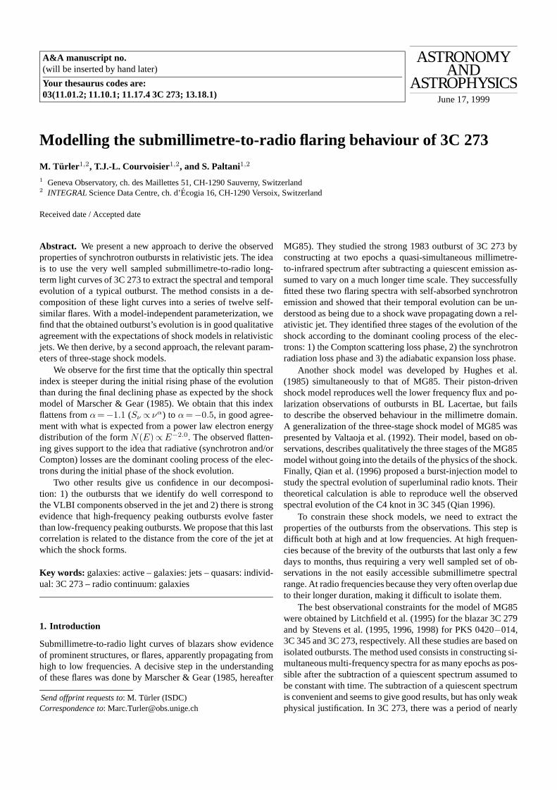
A&A manuscript no.(will be inserted by hand later)

Your thesaurus codes are:03(11.01.2; 11.10.1; 11.17.4 3C 273; 13.18.1)

ASTRONOMYAND

ASTROPHYSICSJune 17, 1999

Modelling the submillimetre-to-radio flaring behaviour of 3C 273

M. T urler 1,2, T.J.-L. Courvoisier1,2, and S. Paltani1,2

1 Geneva Observatory, ch. des Maillettes 51, CH-1290 Sauverny, Switzerland2 INTEGRALScience Data Centre, ch. d’Ecogia 16, CH-1290 Versoix, Switzerland

Received date / Accepted date

Abstract. We present a new approach to derive the observedproperties of synchrotron outbursts in relativistic jets. The ideais to use the very well sampled submillimetre-to-radio long-term light curves of 3C 273 to extract the spectral and temporalevolution of a typical outburst. The method consists in a de-composition of these light curves into a series of twelve self-similar flares. With a model-independent parameterization, wefind that the obtained outburst’s evolution is in good qualitativeagreement with the expectations of shock models in relativisticjets. We then derive, by a second approach, the relevant param-eters of three-stage shock models.

We observe for the first time that the optically thin spectralindex is steeper during the initial rising phase of the evolutionthan during the final declining phase as expected by the shockmodel of Marscher & Gear (1985). We obtain that this indexflattens fromα =−1.1 (Sν ∝ να) to α =−0.5, in good agree-ment with what is expected from a power law electron energydistribution of the formN(E)∝E−2.0. The observed flatten-ing gives support to the idea that radiative (synchrotron and/orCompton) losses are the dominant cooling process of the elec-trons during the initial phase of the shock evolution.

Two other results give us confidence in our decomposi-tion: 1) the outbursts that we identify do well correspond tothe VLBI components observed in the jet and 2) there is strongevidence that high-frequency peaking outbursts evolve fasterthan low-frequency peaking outbursts. We propose that this lastcorrelation is related to the distance from the core of the jet atwhich the shock forms.

Key words: galaxies: active – galaxies: jets – quasars: individ-ual: 3C 273 – radio continuum: galaxies

1. Introduction

Submillimetre-to-radio light curves of blazars show evidenceof prominent structures, or flares, apparently propagating fromhigh to low frequencies. A decisive step in the understandingof these flares was done by Marscher & Gear (1985, hereafter

Send offprint requests to: M. Turler (ISDC)Correspondence to: [email protected]

MG85). They studied the strong 1983 outburst of 3C 273 byconstructing at two epochs a quasi-simultaneous millimetre-to-infrared spectrum after subtracting a quiescent emission as-sumed to vary on a much longer time scale. They successfullyfitted these two flaring spectra with self-absorbed synchrotronemission and showed that their temporal evolution can be un-derstood as being due to a shock wave propagating down a rel-ativistic jet. They identified three stages of the evolution of theshock according to the dominant cooling process of the elec-trons: 1) the Compton scattering loss phase, 2) the synchrotronradiation loss phase and 3) the adiabatic expansion loss phase.

Another shock model was developed by Hughes et al.(1985) simultaneously to that of MG85. Their piston-drivenshock model reproduces well the lower frequency flux and po-larization observations of outbursts in BL Lacertae, but failsto describe the observed behaviour in the millimetre domain.A generalization of the three-stage shock model of MG85 waspresented by Valtaoja et al. (1992). Their model, based on ob-servations, describes qualitatively the three stages of the MG85model without going into the details of the physics of the shock.Finally, Qian et al. (1996) proposed a burst-injection model tostudy the spectral evolution of superluminal radio knots. Theirtheoretical calculation is able to reproduce well the observedspectral evolution of the C4 knot in 3C 345 (Qian 1996).

To constrain these shock models, we need to extract theproperties of the outbursts from the observations. This step isdifficult both at high and at low frequencies. At high frequen-cies because of the brevity of the outbursts that last only a fewdays to months, thus requiring a very well sampled set of ob-servations in the not easily accessible submillimetre spectralrange. At radio frequencies because they very often overlap dueto their longer duration, making it difficult to isolate them.

The best observational constraints for the model of MG85were obtained by Litchfield et al. (1995) for the blazar 3C 279and by Stevens et al. (1995, 1996, 1998) for PKS 0420−014,3C 345 and 3C 273, respectively. All these studies are based onisolated outbursts. The method used consists in constructing si-multaneous multi-frequency spectra for as many epochs as pos-sible after the subtraction of a quiescent spectrum assumed tobe constant with time. The subtraction of a quiescent spectrumis convenient and seems to give good results, but has only weakphysical justification. In 3C 273, there was a period of nearly

2 M. Turler et al.: Modelling the submillimetre-to-radio flaring behaviour of 3C 273

constant flux at millimetre frequencies lasting just more thanone year in 1989–1990, which was interpreted as its quiescentstate (Robson et al. 1993). At radio frequencies, however, nosimilar constant flux period was ever observed and there is noevidence that such a state exists at a significant level above thecontribution of the jet’s hot spot 3C 273A (see Fig. 2 of Türleret al. 1999a).

The different approach presented here to derive the ob-served properties of the outbursts has the advantage to not relyon the assumption of a quiescent emission. The idea is to de-compose a set of light curves covering a large time span intoa series of flares. To our knowledge, the first attempt of sucha decomposition was made by Legg (1984), who fitted a tenyears radio light curve of 3C 120 with twelve self-similar out-bursts. Recently, Valtaoja et al. (1999) decomposed the 22 GHzand 37 GHz radio light curves of many active galactic nucleiinto several exponentially rising and decaying outbursts. Whatis new in our approach is that we fit the same outbursts simulta-neously to twelve light curves covering more than two decadesof frequency from the submillimetre to the radio domain. Thisadds a new dimension to the decomposition: the evolution of aflare is now a function of both time and frequency. The aim isto obtain both the spectral and temporal properties of a typicalflare, from which individual flares differ only by a few param-eters.

We use the light curves of 3C 273, the best observed quasar,to have as many observational constraints as possible. The flar-ing behaviour of 3C 273 was already the subject of several pre-vious studies (e.g. Robson et al. 1993; Stevens et al. 1998).Stevens et al. (1998) obtain results for the first stage of thestrong 1995 flare in very good agreement with the predictionsof the MG85 shock model. The new approach presented here ishowever more powerful to constrain the two following stagesof the evolution.

We describe below two different approaches. In Sect. 3 wemodel the light curve of each outburst by an analytic functionthat can smoothly evolve with frequency, whereas in Sect. 4we directly model a self-absorbed synchrotron spectrum thatevolves with time. The first approach is easier to implement,since it allows us to begin the decomposition with a single lightcurve before adding the others progressively. The second ap-proach is more physical and gives better constraints to shockmodels. Our results are discussed in Sect. 5 and summarized inSect. 6.

Throughout this paper the frequencyν is as measured inthe observer’s frame and “log” refers to the decimal logarithm“ log10”. The convention for the spectral indexα is Sν∝ν+α.

2. Observational material

This study is based on the light curves of the multi-wavelengthdatabase of 3C 273 presented by Türler et al. (1999a). Thetwelve light curves we use are the five radio light curves:5 GHz, 8.0 GHz, 15 GHz, 22 GHz and 37 GHz and the sevenmillimetre/submillimetre (mm/submm) light curves: 3.3 mm,2.0 mm, 1.3 mm, 1.1 mm, 0.8 mm, 0.45 mm and 0.35 mm. At

low frequency (5 to 15 GHz), we consider only the measure-ments of the University of Michigan Radio Astronomy Ob-servatory (UMRAO). The observations at 22 GHz and 37 GHzare mainly from the Metsähovi Radio Observatory in Fin-land. The mm/submm observations are from various sourcesincluding the James Clerk Maxwell Telescope (JCMT), theSwedish-ESO Submillimetre Telescope (SEST) and the “Insti-tut de Radio-Astronomie Millimétrique” (IRAM).

We analyse the observations from 1979.0 to 1996.6, exceptat low frequency where we extend the analysis up to: 1997.2(15 GHz), 1997.5 (8.0 GHz) and 1998.0 (5 GHz), in order toinclude the decay of the 1995 flare. In the mm/submm range,we average repeated observations made within 3 days to avoidoversampling of the light curves at some epochs. This leavesus a total of 4352 observational points to constrain our fits. Toobservations without known uncertainties, we assign the aver-age uncertainty of the other observations at the same frequency.The light curves are treated as if all their observations weremade exactly at the same frequency, i.e. small differences ofthe observing frequency from one measurement to the otherare not taken into account. This simplification should not muchaffect the results, since the spectrum is rather flat (α >∼ − 0.5)in the considered submillimetre-to-radio domain (e.g. Türler etal. 1999a).

3. The light-curve approach

We describe here an approach in which we minimize the num-ber of model-dependent constraints. The light curve of eachoutburst at a given frequency is described by a simple analyt-ical function. The choice of this function is purely empiricaland does not rely on any physical model. The evolution withfrequency of the outburst’s light curve is left as free as possi-ble. This model has therefore many free parameters, which canadapt to a wide range of different situations.

3.1. Number of outbursts

One crucial parameter of the decomposition is the number ofoutbursts. Pushed by the wish to reproduce the small featuresseen in the light curves, one is tempted to add always moreoutbursts to the fit. In Türler et al. (1999b), we published theresults of a decomposition into nineteen outbursts using an ap-proach which is similar to that described below. Here, we tryto minimize as much as possible the number of outbursts tobetter constrain their spectral and temporal evolution. We endwith twelve flares, which are absolutely necessary to describethe main features of the light curves.

The aim of the decomposition is not to reproduce the de-tailed structure of the light curves, but to derive the main char-acteristics of the outbursts. As a consequence, theχ2 that weshall obtain will be statistically completely unacceptable andwill have no meaning in terms of the probability that the modelcorresponds to what is observed. We will however refer to theobtained values of the reducedχ2 (cf. Sect. 3.3), because it isthe usual way to express the quality of a fit.

M. Turler et al.: Modelling the submillimetre-to-radio flaring behaviour of 3C 273 3

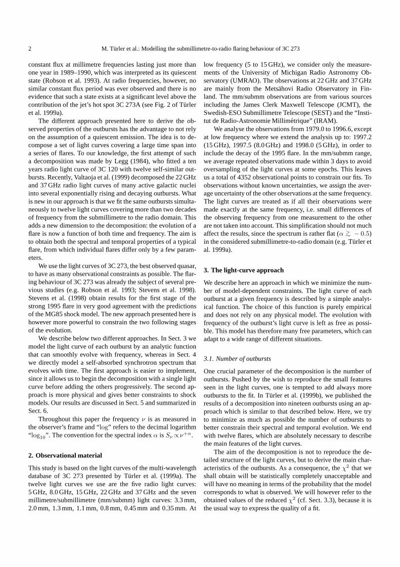
Fig. 1. Model light curve of an outburst defined by Eqs. (1) and (2),which starts at timet0 =0 and peaks at an amplitude ofA(ν)=1 Jy.The three different line types show the effect of varyingρ(ν) andφ(ν)

3.2. Parameterization

At a given frequencyν, we model the light curveSν(t) of asingle outburst of amplitudeA(ν), starting at timet = t0 andpeaking att = t0 + trise(ν) by

Sν(t) =A(ν)

2

[1− cos

(π

(t− t0trise(ν)

)ρ(ν))]

, (1)

if t0 ≤ t < t0 + trise(ν) and by

Sν(t) = A(ν) exp

(−(

t−t0−trise(ν)tfall(ν)

)φ(ν))

, (2)

if t ≥ t0 + trise(ν). The exponentsρ(ν) andφ(ν) define theshape of the light curve at frequencyν and tfall(ν) is the e-folding decay time of the flare at frequencyν. Different timeprofiles of an outburst defined by Eqs. (1) and (2) are shown inFig. 1.

Rather than constraining the outburst parameters (A(ν),trise(ν), tfall(ν), ρ(ν) and φ(ν)) at each of the twelve lightcurve’s frequencies, we describe their logarithm by a cu-bic spline which we parameterize at only four frequenciesspaced by 0.75 dex and covering the 3 – 600 GHz range (seeFig. 3). This reduces the number of free parameters by a factorthree, while keeping the parameterization completely model-independent. We thus need a total of5×4 parameters to fullycharacterize the spectral and temporal evolution of an out-burst, i.e. a surface in the three dimensional(S, ν, t)-space (cf.Fig. 4).

We impose that all individual outbursts are self-similar, inthe sense that they all have the same evolution pattern, i.e. thesame shape of the surface in the(S, ν, t)-space. What we al-low to change from one outburst to the other is the normaliza-tion in flux S, frequencyν and timet, which changes, respec-tively, the amplitude of the outburst (strong or weak), the fre-quency at which the emission peaks (high- or low-frequencypeaking) and the time scale of the evolution (long-lived orshort-lived). A change in normalization corresponds to a shiftof the position of the outburst’s characteristic surface in the(log S, log ν, log t)-space. To define this position, we take thepoint of maximum flux as an arbitrary reference point on thesurface. On average among all individual outbursts, this pointis located at(〈log S〉, 〈log ν〉, 〈log t〉) and this average normal-ization defines what we call thetypical outburstof 3C 273.We denote by∆ log S, ∆ log ν and ∆ log t the logarithmicshifts of this point with respect to the average position, i.e.∆ log k = log k − 〈log k〉, ∀ k = S, ν, t. These12×3 loga-rithmic shifts plus the12 different start timest0 of the flaresgive a total of48 parameters used to define the specificity of alloutbursts.

The superimposed decays of the outbursts that started be-fore 1979 are simply modelled by an hypothetical event of am-plitude A0(ν) at time t = t0 + trise(ν) = 1979.0 and de-caying with thee-folding time tfall(ν) of the typical outburstat frequencyν. The variation of the amplitudeA0(ν) withfrequency is modelled by a cubic spline as for the five othervariables, but parameterized at four slightly lower frequencies(log (ν/GHz) = 0.5, 1.0, 1.5 and 2.0), due to the fact thatA0(ν) is only well constrained for the radio light curves. Fi-nally, we assume a constant contribution to the light curves dueto the quiescent emission of the jet’s hot spot 3C 273A. Thisemission is modelled with a power law spectrum as given inTurler et al. (1999a).

To summarize, this first parameterization uses a total of72(20+48+4) parameters to adjust the 4352 observational pointsin the twelve light curves. The great number of free parametersstill leaves more than four thousand degrees of freedom (d.o.f.)to the fit. The simultaneous fitting of the twelve light curvesis performed by many iterative fits of small subsets of the72parameters.

3.3. Results

Fig. 2 shows three representative light curves among the twelvefitted simultaneously with the outbursts parameterized as de-scribed in Sect. 3.2. The major features of the light curves arereproduced by the model with only about one outburst every1.5 year starting simultaneously at all frequencies. The overallfit has a reducedχ2 value ofχ2

red≡χ2/d.o.f.=16.1. The maindiscrepancy between the model and the observations arises dur-ing 1984–1985, when the very different light curve features inthe millimetre and radio domains cannot be correctly describedby the 1983.4 flare alone.

The obtained evolution of the parameters with frequencyfor the typical outburst is shown in Fig. 3. The amplitude


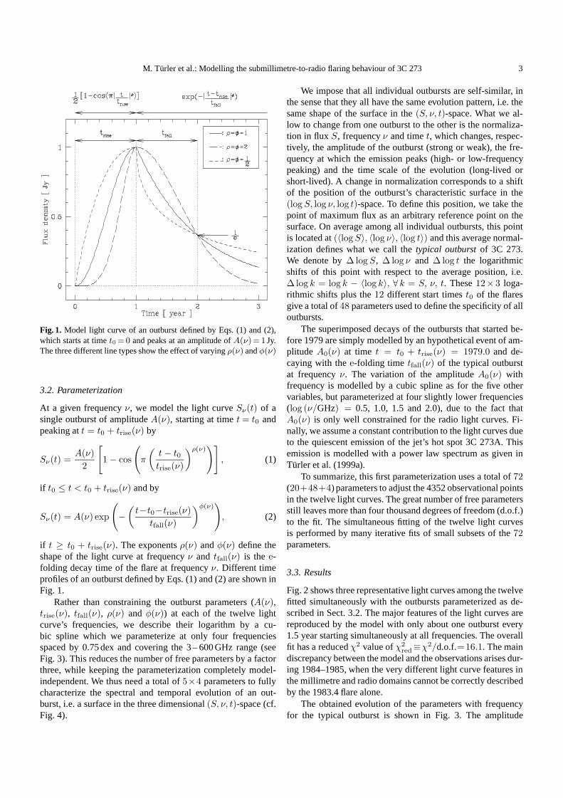
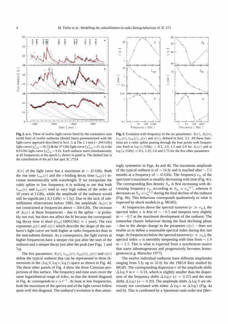
Fig. 2. a–c.Three of twelve light curves fitted by the cumulative sum(solid line) of twelve outbursts (dotted lines) parameterized with thelight-curve approach described in Sect. 3.a The 1.1 mm (∼280 GHz)light curve (χ2

red =30.5); b the 37 GHz light curve (χ2red =21.4); c the

8.0 GHz light curve (χ2red =9.6). Each outburst starts simultaneously

at all frequencies at the epocht0 shown in panela. The dashed line isthe contribution of the jet’s hot spot 3C 273A

A(ν) of the light curve has a maximum at∼ 45 GHz. Boththe rise timetrise(ν) and thee-folding decay timetfall(ν) in-crease monotonically with wavelength. If we extrapolate thecubic spline to low frequency, it is striking to see that bothtrise(ν) and tfall(ν) tend to very high values of the order of10 years at 1 GHz, while the amplitude of the outburst wouldstill be significant (A(1 GHz)≈ 1 Jy). Due to the lack of sub-millimetre observations before 1981, the amplitudeA0(ν) isnot constrained at frequencies above∼300GHz. The increaseof A0(ν) at these frequencies – due to the spline – is proba-bly not real, but does not affect the fit because the correspond-ing decay time is short (tfall(1000 GHz) ≈ 1 year). The twoexponentsρ(ν) andφ(ν) which describe the shape of the out-burst’s light curve are both higher at radio frequencies than inthe mm/submm domain. As a consequence, the light curves athigher frequencies have a steeper rise just after the start of theoutburst and a steeper decay just after the peak (see Figs. 1 and7a).

The five parametersA(ν), trise(ν), tfall(ν), ρ(ν) andφ(ν)define the typical outburst that can be represented in three di-mensions in the(log S, log ν, log t)-space as shown in Fig. 4d.The three other panels of Fig. 4 show the three Cartesian pro-jections of this surface. The frequency and time axes cover thesame logarithmical range of 4 dex, so that the dotted diagonalin Fig. 4c corresponds toν ∝ t−1. At least at low frequencies,both the maximum of the spectra and of the light curves followquite well this diagonal. The outburst’s evolution is thus amaz-

Fig. 3. Evolution with frequency of the six parameters:A(ν), A0(ν),trise(ν), tfall(ν), ρ(ν) andφ(ν), defined in Sect. 3.2. All these func-tions are a cubic spline passing through the four points with frequen-cies fixed atlog (ν/GHz) = 0.5, 1.0, 1.5 and 2.0 forA0(ν) and atlog (ν/GHz) ' 0.5, 1.25, 2.0 and 2.75 for the five other parameters

ingly symmetric in Figs. 4a and 4b. The maximum amplitudeof the typical outburst is of∼ 16 Jy and is reached after∼ 7.5months at a frequency of∼ 45 GHz. The frequencyνm of thespectrum’s maximum is steadily decreasing with time (Fig. 4c).The corresponding flux densitySm is first increasing with de-creasing frequencyνm according toSm ∝ ν−0.7

m , whereas itdecreases asSm∝ν+1.0

m during the final decline of the outburst(Fig. 4b). This behaviour corresponds qualitatively to what isexpected by shock models (e.g. MG85).

At frequencies above the spectral turnover (ν � νm), thespectral indexα is first of∼ −0.5 and steepens very slightlyto ∼ −0.7 at the maximum development of the outburst. Thesomewhat chaotic behaviour during the final declining phase– due to the abrupt change in the parameterφ(ν) – does notenable us to define a reasonable spectral index during this laststage. At frequencies below the spectral turnover (ν � νm), thespectral indexα is smoothly steepening with time from∼ 1.8to ∼ 2.5. This is what is expected from a synchrotron sourcethat starts inhomogeneous and progressively becomes homo-geneous (e.g. Marscher 1977).

The twelve individual outbursts have different amplitudesranging from 5 Jy up to 32 Jy for the 1983.0 flare studied byMG85. The corresponding dispersionσ of the amplitude shifts∆ log S is σ = 0.23, which is slightly smaller than the disper-sion of the frequency shifts∆ log ν (σ = 0.27) and the timeshifts∆ log t (σ = 0.29). The amplitude shifts∆ log S are ob-viously not correlated with either∆ log ν or ∆ log t (Fig. 4aand b). This is confirmed by a Spearman rank-order test (Bev-


Fig. 4. a–d.Logarithmic spectral and tem-poral evolution of the typical outburst ob-tained by the light-curve approach de-scribed in Sect. 3. Paneld shows thethree-dimensional representation in the(log S, log ν, log t)-space. The other panelsshow the three Cartesian projections:a lightcurves at different frequencies spaced by0.2 dex;b spectra at different times spacedby 0.2 dex;c contour plot in the frequencyversus time plan. The thick solid and dashedlines show the evolution of the maximum ofthe spectra and of the light curves, respec-tively. They follow quite well the dotted di-agonal in panelc corresponding toν∝ t−1.The star dot shows the point of maximumdevelopment of the typical outburst. Theopen circles show for each outburst the po-sition that would have this maximum ac-cording to the shifts∆ log S, ∆log ν and∆log t. The arrows in panelb show thefrequency distribution of the twelve lightcurves

ington 1969), which yields that the observed correlations couldoccur by chance with a probability of more than 60 %. On thecontrary, the shifts∆ log ν and ∆ log t align well along theν ∝ t−1 line (Fig. 4c) and the Spearman’s test probability of< 0.01 % confirms that this anti-correlation is very significant.

4. The three-stage approach

In the light-curve approach described above, we model analyt-ically the light curve of an outburst at different frequencies andshow that the resulting typical flare is qualitatively in agree-ment with what is expected by shock models in relativistic jets.It is thus of interest to derive from the data the parameters thatare relevant to those models.

The shock model of MG85 and its generalization by Val-taoja et al. (1992) describe the evolution of the shock by threedistinct stages: 1) a rising phase, 2) a peaking phase and 3) adeclining phase1. The three-stage approach presented below issimilar to that of Valtaoja et al. (1992), in the sense that its aimis simply to qualitatively describe the observations. It containshowever more parameters in order to include those which arerelevant to test the physical model of MG85.

1 We use here the terminology introduced by Qian et al. (1996),because it is purely descriptive and free of any interpretation regardingthe physical origin of these stages.

The remarks of Sect. 3.1 concerning the number of out-bursts and the quoted values of the reducedχ2 apply equallyhere.

4.1. Parameterization

The self-absorbed synchrotron spectrum emitted by electronswith a power law energy distribution of the formN(E)∝E−s

can be expressed – by generalizing the homogeneous case (e.g.Pacholczyk 1970; Stevens et al. 1995) – as

Sν = S1

(ν

ν1

)αthick 1− exp (−(ν/ν1)αthin−αthick)1− e−1

, (3)

where(ν/ν1)αthin−αthick is equal to the optical depthτν at fre-quencyν. S1 andν1 are respectively the flux density and thefrequency corresponding to an optical depth ofτν =1. At highfrequency (ν� ν1) the medium is optically thin (τν � 1) andthe spectrum follows a power law of indexαthin =−(s−1)/2,whereas at low frequency (ν�ν1) it is optically thick (τν�1)and the spectral index isαthick. In the case of a homogeneoussource,αthick =+5/2.

The maximumSm≡Sν(νm) of the spectrumSν is reachedat the turnover frequencyνm corresponding to an optical depth


of τm = (νm/ν1)αthin−αthick . τm is obtained by differentiatingEq. (3):

dSν

dν= 0 ⇒ exp (τm)− 1 =

(1− αthin

αthick

)τm . (4)

By developing the exponential of Eq. (4) to the third order, we

obtain a good approximate:τm = 32

(√1− 8 αthin

3 αthick− 1)

. We

can now rewrite Eq. (3) according to the turnover valuesνm,τm andSm by

Sν = Sm

(ν

νm

)αthick 1− exp (−τm (ν/νm)αthin−αthick)1− e−τm

. (5)

The evolution with time of the self-absorbed synchrotronspectrum of Eq. (5) is assumed to follow three distinct stages:1) the rising phase fort− t0 < tr ; 2) the peaking phase fortr ≤ t− t0 ≤ tp and 3) the declining phase fort− t0 > tp.The subscripts “r” and “p” refer to the end of the rising phaseand the end of the peaking phase, respectively. We assume thatduring each stagei (i = 1, 2, 3) both the turnover frequencyνm(t) and the turnover fluxSm(t) evolve with time as a powerlaw, but with exponents that differ during the three stages:

νm(t) ∝ tβi and Sm(t) ∝ tγi ⇒ Sm ∝ νγi/βim . (6)

We thus need ten parameters:tr, tp, νm(tr), Sm(tr), β1, β2, β3,γ1, γ2 andγ3, to describe the evolution of the spectral turnoverin the three dimensional(S, ν, t)-space.

The model of MG85 predicts that both the optically thinαthin and thickαthick spectral indices should be flatter duringthe declining phase than during the rising and peaking phases(see Fig. 3 of Marscher et al. 1992). To test whether the spec-trum is actually changing from the rising phase to the decliningphase, we allow the two spectral indicesαthin andαthick tohave different values during these two stages. The transitionduring the intermediate peaking phase from the values in therising phase (αthin(tr) andαthick(tr)) to the values in the de-clining phase (αthin(tp) andαthick(tp)) is assumed to be linearwith the logarithm of timelog (t). This adds the four parame-tersαthin(tr), αthin(tp), αthick(tr) andαthick(tp) to the model,having thus a total of fourteen parameters to fully define theevolution of a typical flare in the(S, ν, t)-space instead of thetwenty parameters used in the first approach (Sect. 3.2).

The specificity of each outburst is modelled with a totalof 12×4 parameters exactly as described in Sect. 3.2 for thelight-curve approach. We do not model again the superimposeddecays of the outbursts that started before 1979, but simplyuse the same exponential decay as obtained by the first ap-proach (Sect. 3.2). The constant contribution of the jet’s hotspot 3C 273A is also considered here. The total number of pa-rameters in this second parameterization is a bit less than forthe first one: 62 (12×4 + 14) instead of 72.

4.2. Results

To allow a better comparison with the results of the first ap-proach (Sect. 3.2), we show in Fig. 5 the same light curves as

Fig. 5. a–c.Same as Fig. 2, but with the outbursts parameterized ac-cording to the three-stage approach described in Sect. 4.a The 1.1 mm(∼ 280 GHz) light curve (χ2

red = 26.8); b the 37 GHz light curve(χ2

red =20.4); c the 8.0 GHz light curve (χ2red =10.9)

Table 1. Values of the parameters defined in Sect. 4.1 correspondingto the evolution of the typical outburst shown in Fig. 6. The two firstcolumns display the fourteen best fit parameters, whereas other relatedparameters are shown in the last column

Param. Value Param. Value Param. Value

tr 0.14 year tp 1.63 yearνm(tr) 120 GHz νm(tp) 13.8 GHzSm(tr) 15.3 Jy Sm(tp) 15.9 Jyαthin(tr) −1.09 αthin(tp) −0.48αthick(tr) +1.55 αthick(tp) +1.74β1 −0.51 γ1 +0.51 γ1/β1 −0.99β2 −0.88 γ2 +0.02 γ2/β2 −0.02β3 −1.19 γ3 −1.36 γ3/β3 +1.14

in Fig. 2. The reducedχ2 of the overall fit is now ofχ2red =17.8.

The higher frequency light curves are relatively better de-scribed here than with the first approach (compare Figs. 2 and5). The start timest0 of the outbursts are very similar to thoseobtained by the first approach, except for the fourth flare whichis now starting much later att0 = 1984.1 instead of 1983.4. Thislater t0 seems to be in better agreement with the observations,but the behaviour of 3C 273 during 1984–1985 is still poorlydescribed.

The obtained values of the parameters are given in Table 1.They correspond to the spectral and temporal evolution of thetypical outburst shown in Fig. 6. If the tracks followed by themaximum of the spectra and of the light curves are similarto those obtained by the first approach (Fig. 4), the spectral


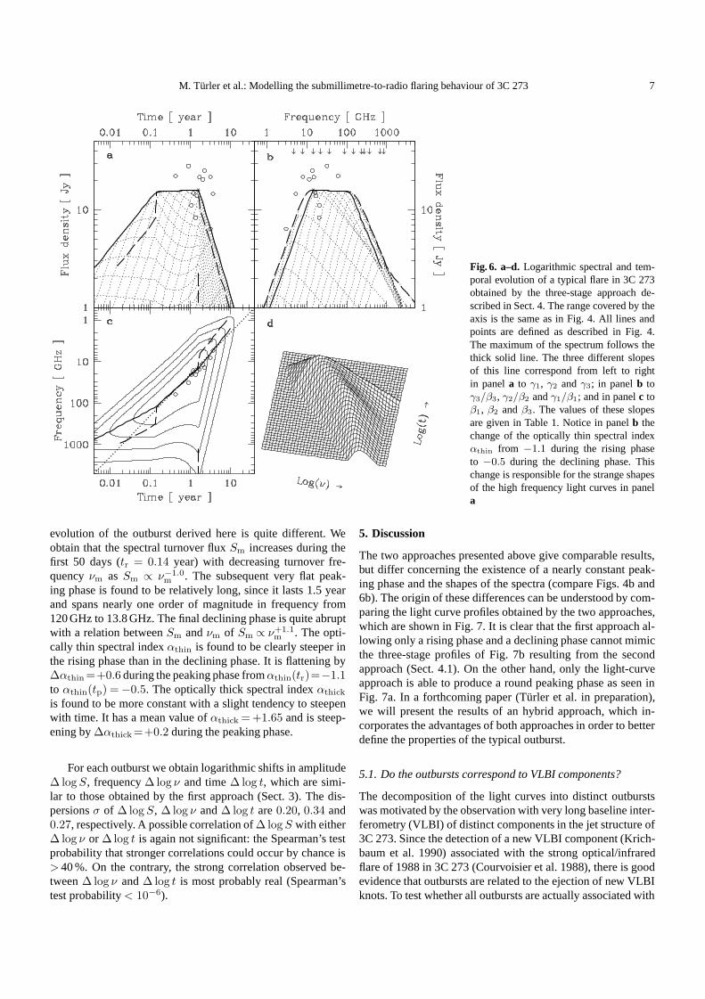
Fig. 6. a–d.Logarithmic spectral and tem-poral evolution of a typical flare in 3C 273obtained by the three-stage approach de-scribed in Sect. 4. The range covered by theaxis is the same as in Fig. 4. All lines andpoints are defined as described in Fig. 4.The maximum of the spectrum follows thethick solid line. The three different slopesof this line correspond from left to rightin panela to γ1, γ2 andγ3; in panelb toγ3/β3, γ2/β2 andγ1/β1; and in panelc toβ1, β2 andβ3. The values of these slopesare given in Table 1. Notice in panelb thechange of the optically thin spectral indexαthin from −1.1 during the rising phaseto −0.5 during the declining phase. Thischange is responsible for the strange shapesof the high frequency light curves in panela

evolution of the outburst derived here is quite different. Weobtain that the spectral turnover fluxSm increases during thefirst 50 days (tr = 0.14 year) with decreasing turnover fre-quencyνm as Sm ∝ ν−1.0

m . The subsequent very flat peak-ing phase is found to be relatively long, since it lasts 1.5 yearand spans nearly one order of magnitude in frequency from120 GHz to 13.8 GHz. The final declining phase is quite abruptwith a relation betweenSm andνm of Sm ∝ ν+1.1

m . The opti-cally thin spectral indexαthin is found to be clearly steeper inthe rising phase than in the declining phase. It is flattening by∆αthin =+0.6 during the peaking phase fromαthin(tr)=−1.1to αthin(tp) =−0.5. The optically thick spectral indexαthick

is found to be more constant with a slight tendency to steepenwith time. It has a mean value ofαthick = +1.65 and is steep-ening by∆αthick =+0.2 during the peaking phase.

For each outburst we obtain logarithmic shifts in amplitude∆ log S, frequency∆ log ν and time∆ log t, which are simi-lar to those obtained by the first approach (Sect. 3). The dis-persionsσ of ∆ log S, ∆ log ν and∆ log t are0.20, 0.34 and0.27, respectively. A possible correlation of∆ log S with either∆ log ν or ∆ log t is again not significant: the Spearman’s testprobability that stronger correlations could occur by chance is> 40 %. On the contrary, the strong correlation observed be-tween∆ log ν and∆ log t is most probably real (Spearman’stest probability< 10−6).

5. Discussion

The two approaches presented above give comparable results,but differ concerning the existence of a nearly constant peak-ing phase and the shapes of the spectra (compare Figs. 4b and6b). The origin of these differences can be understood by com-paring the light curve profiles obtained by the two approaches,which are shown in Fig. 7. It is clear that the first approach al-lowing only a rising phase and a declining phase cannot mimicthe three-stage profiles of Fig. 7b resulting from the secondapproach (Sect. 4.1). On the other hand, only the light-curveapproach is able to produce a round peaking phase as seen inFig. 7a. In a forthcoming paper (Türler et al. in preparation),we will present the results of an hybrid approach, which in-corporates the advantages of both approaches in order to betterdefine the properties of the typical outburst.

5.1. Do the outbursts correspond to VLBI components?

The decomposition of the light curves into distinct outburstswas motivated by the observation with very long baseline inter-ferometry (VLBI) of distinct components in the jet structure of3C 273. Since the detection of a new VLBI component (Krich-baum et al. 1990) associated with the strong optical/infraredflare of 1988 in 3C 273 (Courvoisier et al. 1988), there is goodevidence that outbursts are related to the ejection of new VLBIknots. To test whether all outbursts are actually associated with


Fig. 7. a and b.Light curves at different frequencies for the typicaloutburst obtained with the light-curve approach (a) and the three-stageapproach (b). The dotted light curves are spaced by 0.1 dex in fre-quency and the six solid light curves are at frequencieslog (ν/GHz)=3.0, 2.5, . . . , 0.5, in order of increasing time scales

superluminal components, we compare in Table 2 the start timet0 of an outburst – as obtained by the three-stage approach –with the ejection time “t0 (knot)” of a new VLBI knot as givenby Abraham et al. (1996) and Zensus et al. (1990). For eachof the eight first outbursts, we can identify one or two possiblyassociated VLBI components.

To test further this relationship, we compare the flux densi-ties “Fobs (knot)” of the VLBI components observed at epocht = 1991.15 and at a frequency of 10.7 GHz (Abraham et al.1996) with the flux densitiesFexp(t=1991.15, ν =10.7 GHz)expected at the same epoch and the same frequency accordingto the outburst parameters derived here. Table 2 shows that forthe five first outbursts there is always one of the possibly as-sociated knots (indicated by an arrow), which has the expectedflux. For the three remaining outbursts and especially for the1988.1 flare, the relation betweenFobs (knot) andFexp is notobvious. At this epoch however, the possibly associated com-ponents are still strongly blended by the core emission (com-ponent “D”) or might even still be part of the unresolved core2.The total fluxFexp = 20.9 Jy expected by the 1986.3, 1988.1and 1990.3 outbursts is indeed equal to the observed total fluxFobs =21.4± 0.7 Jy of the C9, C10 and D components. Theseresults strongly suggest that there is a close relation betweenthe outbursts and the VLBI knots and hence that our decompo-sition describes a real physical aspect of the jet.

2 In our model the core emission is entirely due to a superimpositionof outbursts unresolved by the VLBI.

Table 2. Relation between VLBI components and the eight first out-bursts as obtained with the three-stage approach (Sect. 4). The param-eters in this table are defined in Sect. 5.1

t0 Knot t0 (knot) Fexp Fobs (knot)

1979.6 C5 1978.6±0.04 0.4 Jy 0.7± 0.4 Jy←C6 1980.0±0.04 1.9± 0.5 Jy

1980.9 C6 1980.0±0.04 1.9 Jy 1.9± 0.5 Jy←X < 1985.6 < 0.5 Jy

1982.4 C7 1982.2± 0.4 0.2 Jy < 0.5 Jy←1983.1 C7a 1983.1±0.00 0.9 Jy < 0.5 Jy

C7b 1983.6±0.09 1.2± 0.3 Jy←1984.1 C7b 1983.6±0.09 3.8 Jy 1.2± 0.3 Jy

C8 1984.7±0.10 4.4± 0.5 Jy←1986.3 Cx < 1988.2 1.0 Jy < 0.5 Jy1988.1 C9 1988.4±0.17 11.2 Jy 1.8± 0.4 Jy1990.3 C10 < 1990.2 8.7 Jy 6.4± 0.5 Jy

D 13.2± 0.3 Jy

5.2. How can we understand the peculiarities of individualoutbursts?

The relation found between the outbursts and the VLBI knots(Sect. 5.1) has established that our decomposition is notpurely mathematical, but does correspond to a physical real-ity. There should therefore be a physical origin to the clearanti-correlation found between the frequency shifts∆ log νand the time shifts∆ log t of the individual outbursts. Theobserved frequency shifts∆ log ν confirm that 3C 273 emitsboth low- and high-frequency peaking outbursts (Lainela etal. 1992). The relation between∆ log ν and ∆ log t clearlyshows that high-frequency peaking flares evolve faster thanlow-frequency peaking outbursts. The alignment of the shiftsalong theν ∝ t−1 line (Figs. 4c and 6c) further suggests therelation∆ log ν =−∆ log t.

The origin of this relation could be due to a change∆ logDof the Doppler factorD = γ−1(1 − β cos θ)−1, which de-pends on the flow speedβ = v/c, the Lorentz factorγ =(1 − β2)−1/2 and the angle to the line of sightθ. Observedquantities (unprimed) are related to emitted quantities (primed)as (e.g. Hughes & Miller 1991; Pearson & Zensus 1987):

ν = D ν′ ⇒ ∆ log ν = ∆ logD + ∆ log ν′ (7)

t = D−1 t′ ⇒ ∆ log t = −∆ logD + ∆ log t′ (8)

S(ν) = D3 S′(ν′) ⇒ ∆ log S = 3 ∆ logD + ∆ log S′ (9)

If we assume that in the jet frame all outbursts are alike (i.e.∆ log k′ = 0, ∀ k = S, ν, t), the observed relation∆ log ν =−∆ log t can be interpreted as a change∆ logD of the Dopplerfactor from one outburst to the other. In this case, however,there should also be correlations between∆ log S and both∆ log ν and∆ log t, which are not observed.

Alternatively, we can consider that the Doppler factor doesnot change (∆ logD = 0) and that the observed relation be-tween∆ log ν and∆ log t is intrinsic and independent of pos-sible flux variations∆ log S. Such a correlation might be re-


Fig. 8. Schematic representation of a conical jet with constant speedv in which the frequency of maximum emissionνm (greyscale) is in-versely proportional to the distance down the jetr=v t (νm∝r−1 ∝t−1). Let us assume that the peaking phase of an outburst correspondsto an octave of radius (r → 2 r). This phase has a duration and afrequency range which clearly depend on the distancer0 at whichthe shock forms. Inner outbursts peaking fromr∗/2 to r∗ are fourtimes shorter than outer outbursts peaking from2 r∗ to 4 r∗, whiletheir emission is maximum at four times higher frequencies

lated to the distance from the core at which the shock forms(Lainela et al. 1992). Indeed, Blandford (1990) shows that fora simple conical jet with constant speedv the frequency ofmaximum emissionνm is inversely proportional to the dis-tance down the jetr=v t (νm∝ r−1), while the correspondingflux densitySm is constant. Since the speedv is constant, theturnover frequencyνm is then also inversely proportional totime (νm ∝ t−1), as observed. If a shock forms in such an un-derlying jet at a distancer0 from the core, both the frequencyrange of the emission and the time scale of the evolution willdepend on the distancer0, as illustrated in Fig. 8. We thereforepropose that short-lived and high-frequency peaking flares areactuallyinneroutbursts, whereas long-lived and low-frequencypeaking flares areouteroutbursts.

This interpretation is supported by the existence of short-lived VLBI components which are only seen close to the core.In our decomposition, the two most short-lived and the mosthigh-frequency peaking outbursts are the two successive flaresof 1982.4 and 1983.1. Their start times correspond well to theperiod from 1981 to 1983 during which only short-lived VLBIcomponents were formed (Abraham et al. 1996). If our inter-pretation is right, the shifts∆ log ν and∆ log t that we obtainsuggest that the 1982.4 flare would have formed about twotimes closer to the core than the 1983.1 flare and four timescloser than the typical outburst.

5.3. What are the constraints for shock models?

According to the shock model of MG85, the optically thinspectral indexαthin should be steeper during the two firststages of the outburst evolution than the usual value ofαthin=−(s − 1)/2 (Sect. 4.1). A steeper index arises due to the factthat the thicknessx of the emitting region behind the shockfront is proportional to the cooling timetcool of the electronssuffering radiative (Compton and/or synchrotron) losses. Dur-ing the rising and peaking phases, radiative losses are domi-nant and therefore the thicknessx is frequency dependent asx∝ tcool∝ ν−1/2, which leads to a steeper optically thin spec-tral index ofαthin =−s/2. Until now, the expected flatteningof the spectral index by∆αthin = +0.5 from the rising andpeaking phases to the declining phase was never observed andfurthermore the optically thin spectral indexαthin observed atthe beginning of the outburst was often found to be already tooflat (αthin>−1/2) to allow the expected subsequent flattening(Valtaoja et al. 1988; Lainela 1994).

The present result that the optically thin spectral index isflattening with time by∆αthin = +0.6 is in good agreementwith the change of∆αthin =+0.5 expected by the shock modelof MG85. The observed flattening of the spectrum is contraryto the steepening with time expected as a result of radiative en-ergy losses by the electrons. The observed behaviour can how-ever also be understood as a change of slope with frequencyrather than with time and thus it could conceivably be due to aspectral break that steepens the optically thin spectral index bya factor of 0.5 at higher frequencies. Such a break is expected inthe case of continuous injection or reacceleration of electronssuffering radiative losses (Kardashev 1962) and is observedin several hot spots including 3C 273A (Meisenheimer et al.1989). Whatever the interpretation, the flatter index,αthin(tp),is the relevant index to determine that the electron energy in-dexs (N(E)∝E−s) is s=1 − 2 αthin(tp)=+2.0. This valuecorresponds to the average value observed in several hot spots(Meisenheimer et al. 1989) and is in agreement with the valuesexpected if the electrons are accelerated by a Fermi mechanismin a relativistic shock (e.g. Longair 1994).

The long flat peaking phase observed in 3C 273 contrastswith the complete absence of this stage in 3C 345 (Stevenset al. 1996). This difference is surprising, because the out-burst’s evolution is otherwise very similar in these two objectswith nearly the same indices for the rising and the decliningphases:γ1/β1 = −0.99 in 3C 273 and−0.86 in 3C 345 and

γ3/β3 =+1.14 in 3C 273 and+0.98 in 3C 345 (Sm∝νγi/βim ).

A value ofγ3/β3∼+1 was also found in several other sourcesby Valtaoja et al. (1988). This decrease of the turnover fluxwith decreasing frequency is steeper than expected by the sim-plest model of MG85; i.e. with a conical adiabatic jet havinga constant Doppler factorD. With s = 2 and a magnetic fieldB oriented perpendicular to the jet axis, their model predictsγ3/β3 =+0.45. This discrepancy between the observations andthe shock model of MG85 was already pointed out by Stevenset al. (1996). We refer the reader to their discussion of two moregeneral cases of the MG85 model: 1) a straight non-adiabatic


jet and 2) a curved adiabatic jet. With the observed values of theindicesβ3 andγ3, these authors could determine the two freeparameters of the model. In our case, with the constraints of allsix indicesβi andγi (i = 1, 2, 3), we could not find a goodagreement with either of the two models mentioned above. Ina forthcoming paper (Türler et al. in preparation), we will fur-ther discuss this point and explore whether a non-conical non-adiabatic curved jet can well describe the observations.

6. Summary and conclusion

By using most available submillimetre-to-radio observations of3C 273, we have been able to extract the properties of the spec-tral and temporal evolution of a typical outburst. The new ap-proach we defined consists in decomposing the light curves intoseveral self-similar outbursts. The main results of our decom-position are the followings:

– It is possible to understand the very different shapes of thesubmillimetre-to-radio light curves of 3C 273 with onlyabout one outburst every 1.5 year starting simultaneouslyat all frequencies.

– There is no need to invoke any underlying quiescent emis-sion apart from the weak contribution of the jet’s hot spot3C 273A.

– The outbursts that we identify do well correspond to theobserved VLBI components in the jet.

– There is good evidence that short-lived and high-frequencypeaking flares are emitted closer to the core of the jet thanlong-lived and low-frequency peaking outbursts.

– The spectral and temporal evolution of the outbursts isfound to be in good qualitative agreement with the evolu-tion expected by shock models in relativistic jets.

– We observe a flattening of the optically thin spectral indexfrom the rising to the declining phase of the shock evolu-tion, which supports the idea proposed by MG85 that ra-diative (synchrotron and/or Compton) losses are the maincooling process of the electrons during the initial phase ofthe outburst.

We are aware that our decomposition is far from describingthe detailed structure of the light curves and that the jet emis-sion is much more complicated than this work tries to show.Nevertheless, the results suggest that the outbursts we iden-tified are closely related to the VLBI knots, and hence thatthey describe a physical aspect of the jet. The new approachpresented here is a powerful tool to derive the observed prop-erties of millimetre and radio outbursts. It allows comparisonbetween shock models and the observations and we are con-fident that such decompositions are able to further constrainpresent and future shock models. Finally, we would like tostress the importance of long-term multi-wavelength monitor-ing campaigns, which turn out to be essential towards a betterunderstanding of the physics involved in relativistic jets.

References

Abraham Z., Carrara E.A., Zensus J.A., Unwin S.C., 1996, A&AS115, 543

Bevington P.R., 1969. Data Reduction and Error Analysis for thePhysical Sciences, McGraw-Hill Book Company

Blandford R.D., 1990. In: Active Galactic Nuclei, Courvoisier T.J.-L.,Mayor M. (eds.), Saas-Fee Advanced Course No. 20, Springer-Verlag, p. 161

Courvoisier T.J.-L., Robson E.I., Blecha A., et al., 1988, Nat 335, 330Hughes P.A., Miller L., 1991. In: Beams and Jets in Astrophysics,

Hughes P.A. (ed.), Cambridge Astrophysics Series No. 19, p. 1Hughes P.A., Aller H.D., Aller M.F., 1985, ApJ 298, 301Kardashev N.S., 1962, AZh 39, 393 (SvA 6, 317)Krichbaum T.P., Booth R.S., Kus A.J., et al., 1990, A&A 237, 3Lainela M., 1994, A&A 286, 408Lainela M., Valtaoja E., Tornikoski M., 1992. In: Variability of

Blazars, Valtaoja E., Valtonen M. (eds.), Cambridge Univ. Press,p. 102

Legg T.H., 1984. In: VLBI and Compact Radio Sources, Fanti R.,Kellermann K., Setti G. (eds.), IAU Symposium No. 110, p. 183

Litchfield S.J., Stevens J.A., Robson E.I., Gear W.K., 1995, MNRAS274, 221

Longair M.S., 1994. High Energy Astrophysics, 2nd ed., Vol. 2, Cam-bridge Univ. Press

Marscher A.P., 1977, ApJ 216, 244Marscher A.P., Gear W.K., 1985, ApJ 298, 114 (MG85)Marscher A.P., Gear W.K., Travis J.P., 1992. In: Variability of Blazars,

Valtaoja E., Valtonen M. (eds.), Cambridge Univ. Press, p. 85Meisenheimer K., Röser H.-J., Hiltner P.R., et al., 1989, A&A 219, 63Pacholczyk A.G., 1970. Radio Astrophysics, Freeman, San FranciscoPearson T.J., Zensus J.A., 1987. In: Superluminal Radio Sources, Zen-

sus J.A., Pearson T.J. (eds.), Cambridge Univ. Press, p. 1Qian S.J., 1996, Acta Astrophys. Sin. 16, 143 (Chin. Astron. Astro-

phys. 20, 281)Qian S.J., Witzel A., Britzen S., Krichbaum T.P., Kraus A., 1996. In:

Energy Transport in Radio Galaxies and Quasars, Hardee P.E.,Bridle A.H., Zensus J.A. (eds.), ASP Conf. Series, Vol. 100, p. 61

Robson E.I., Litchfield S.J., Gear W.K., et al., 1993, MNRAS 262, 249Stevens J.A., Litchfield S.J., Robson E.I., et al., 1995, MNRAS 275,

1146Stevens J.A., Litchfield S.J., Robson E.I., et al., 1996, ApJ 466, 158Stevens J.A., Robson E.I., Gear W.K., et al., 1998, ApJ 502, 182Turler M., Paltani S., Courvoisier T.J.-L., et al., 1999a, A&AS 134, 89Turler M., Courvoisier T.J.-L., Paltani S., 1999b. In: BL Lac Phe-

nomenon, Takalo L.O., Sillanpäa A. (eds.), ASP Conf. Series, Vol.159, p. 297

Valtaoja E., Haarala S., Lehto H., et al., 1988, A&A 203, 1Valtaoja E., Teräsranta H., Urpo S., et al., 1992, A&A 254, 71Valtaoja E., Lahteenmäki A., Terasranta H., Lainela M., 1999, ApJS

120, 95Zensus J.A., Unwin S.C., Cohen M.H., Biretta J.A., 1990, AJ 100,

1777

Documents

ASTRONOMY ASTROPHYSICS Modelling the … · constructing at two epochs a quasi-simultaneous millimetre- to-infrared spectrum after subtracting a quiescent emission as- sumed to vary