Astronomy & Astrophysics A 3D MHD model of astrophysical - Sirrah

A&A 369, 706–728 (2001)DOI: 10.1051/0004-6361:20010157c© ESO 2001

Astronomy&

Astrophysics

A 3D MHD model of astrophysical flows: Algorithms, testsand parallelisation

S. E. Caunt and M. J. Korpi

Astronomy Division, Department of Physical Sciences, PO Box 3000, 90014 University of Oulu, Finland

Received 22 December 2000 / Accepted 24 January 2001

Abstract. In this paper we describe a numerical method designed for modelling different kinds of astrophysicalflows in three dimensions. Our method is a standard explicit finite difference method employing the local shearing-box technique. To model the features of astrophysical systems, which are usually compressible, magnetised andturbulent, it is desirable to have high spatial resolution and large domain size to model as many features aspossible, on various scales, within a particular system. In addition, the time-scales involved are usually wide-ranging also requiring significant amounts of CPU time. These two limits (resolution and time-scales) enforcehuge limits on computational capabilities. The model we have developed therefore uses parallel algorithms toincrease the performance of standard serial methods. The aim of this paper is to report the numerical methodswe use and the techniques invoked for parallelising the code. The justification of these methods is given by theextensive tests presented herein.

Key words. magnetohydrodynamics – turbulence – shock waves – methods: numerical – galaxies: ISM – accretion,accretion disks

1. Introduction

Magnetic fields are present everywhere in the universe,for example in planets, stars, accretion disks around com-pact objects, galaxies of various kinds and even in theintergalactic medium. Most of these systems are charac-terised by large kinetic and magnetic Reynolds numbers,indicating that they are highly turbulent, and also thatmagnetic fields are dynamically significant. In many casesthe observed magnetic field has, in addition to a randomsmall-scale component, coherent magnetic field structureson large scales. For example the Sun has a mean magneticfield of dipolar structure, whereas numerous spiral galax-ies posses a mean field of spiral shape often following theoptical spiral arms. One of the fundamental questions inastrophysics is how the order seen in the large scale mag-netic field structures can arise in the turbulent media theyare embedded within.

The most plausible mechanism suggested to explainthis phenomenon is the hydromagnetic dynamo (Parker1955; Steenbeck et al. 1966), according to which large-scale magnetic fields can be generated and maintainedby the combination of turbulence and large-scale shear-ing motions. Based on this theory, a vast number ofmean-field dynamo models, which solve for the large scalemagnetic field with turbulence remaining a parameterised

Send offprint requests to: M. J. Korpi,e-mail: [email protected]

quantity, have been developed for practically all astro-physical objects. Since the form and magnitude of theturbulent quantities are relatively unknown, this param-eterisation is usually kept as simple as possible. The in-formation lacking from these models can be obtained bystudying the non-linear evolution of a magnetised turbu-lent flow in a fully 3D numerical simulation. These kindof simulations (e.g. Balsara & Pouquet 1999; Brandenburg2000) have revealed that in the presence of helical turbu-lence, magnetic field energy can be transferred from thesmallest scales to the larger ones, known as inverse cascade(Frisch et al. 1975; Pouquet et al. 1976). These simula-tions, however, have not yet developed to the stage wherea realistic physical setup for a particular object could bestudied.

On the other hand, when the magnetic field becomesstrong enough it can influence the fluid motions throughthe Lorentz force suppressing turbulence and therebyquenching the generation of magnetic field, known asα-quenching in the mean field dynamo theory. Recentnumerical simulations (Cattaneo & Hughes 1996) have in-dicated that the dynamo α is dramatically quenched im-plying that dynamo action cannot occur in high Reynoldsnumber flows. However, this result is still debatable andrequires investigation under more realistic physical setups(see for example Brandenburg 2000).

Modelling these kinds of systems provides a wide rangeof numerical challenges. One challenge that can never be

S. E. Caunt & M. J. Korpi: 3D MHD model of astrophysical flows 707

overcome satisfactorily is the need for the highest possiblespatial resolution to model turbulence. In some cases eventhe turbulent forcing occurs at very small scales, for exam-ple in galaxies where turbulence is mainly driven by dy-ing stars exploding as supernovae (hereafter SNe). On theother extreme, one would also like to include the largestpossible scales to study not only the generation of large-scale magnetic field, but also large-scale vertical struc-tures such as chimneys or fountains observed in galaxies(e.g. Koo et al. 1992; Normandeau et al. 1996) and az-imuthal features such as field reversals in accretion disks(e.g. Brandenburg et al. 1995; hereafter BNST). Anotherimportant feature of astrophysical flows which has to betaken into account is their compressible nature. With theviolent physical processes active in these flows, such asSNe in galaxies and rapidly growing instabilities like theBalbus-Hawley instability in accretion disks (Balbus &Hawley 1991), shocks are commonly formed. Since thephysical viscosity in the flow is negligible and the physi-cal quantities become discontinuous, additional numericaltechniques are required to resolve them (von Neumann &Richtmyer 1950 hereafter vNR). Once the flow has becometurbulent, the time-scales involved in these turbulent mo-tions is usually much shorter than the orbital period ordecay time-scale of the magnetic field. To study the long-term evolution of the system a huge number of time-stepsmay be required. This all implies the need for efficientalgorithms along with high resolution and large domainsize.

A number of numerical models of this type have beendeveloped being either specifically designed for a partic-ular object (for solar corona e.g. Galsgaard & Nordlund1996, for stellar convection e.g. Stein & Nordlund 1998,for accretion disks e.g. Hawley et al. 1995; BNST, for theinterstellar matter e.g. Rosen & Bregman 1995; Vazquez-Semadeni et al. 1995; Mac Low 1999; Korpi et al. 1999) orbeing more general (Stone & Norman 1992a, 1992b), andmore recently global models are starting to appear (e.g. forthe accretion disks Hawley & Krolik 2000). Our method isbased on the standard local Cartesian shearing-box sim-ulation (e.g. Wisdom & Tremaine 1988) and uses explicitfinite differences on an Eulerian grid, discretising physi-cal quantities onto a uniform mesh, ideal for data paral-lelisation. The methods are in principle very simple andtherefore easy to implement and allow for rapid develop-ment. Shock viscosities (vNR) and further diffusive tech-niques (Nordlund & Galsgaard 1997 hereafter NG; Stein &Nordlund 1998) require additional effort but are howevernecessary to stabilise the numerics.

This paper is structured as follows. Section 2 describesthe essential physics behind our model. Section 3 providesdetails of the numerical methods we use to model the fluidincluding the artificial viscosity employed to resolve shocksand reduce unphysically generated waves and the treat-ment of the boundaries of the box. The parallelisation ofthe code is discussed in Sect. 4 and finally the test suiteused to verify the accuracy and acceptability of the codeis covered in Sect. 5. Finally in Sect. 6 we summarise.

2. The generalised model

2.1. Introduction

In this section we discuss the partial differential equations(PDEs) solved for in all astrophysical systems under con-sideration. These equations describe the flow of a mag-netically conducting fluid within a differentially rotatingbody. Other, more specific, models include extra termsto model effects such as heating by supernovae (hereafterSNe) or stellar winds (hereafter SWs), and suitable cool-ing functions for various systems.

2.2. The non-ideal MHD equations

We solve the standard non-ideal MHD equations in threedimensions using the standard shearing-box techniquesimilar to those used by e.g. BNST and Hawley et al.(1995). The equations are solved in a computational do-main representing a small volume within a differentiallyrotating cosmic object. The coordinate system is reducedto Cartesian with x representing radial, y azimuthal andz vertical direction, the dimensions of the box beingLx × Ly × Lz. The centre of the box is located at dis-tance R from the centre of rotation, which is much largerthan any dimension of the domain. This reference pointis moving on a circular orbit with angular velocity Ω0

around the centre. As the fluid is rotating differentially,the angular velocity is changing as function of distancefrom the centre of rotation. In the local frame of referencethe equations of motion can be linearised relative to thereference point (e.g. Spitzer & Schwarzschild 1953; Julian& Toomre 1966) yielding a solution which can be inter-preted to have two contributions: the circular motion givenby u0 = −2Axy and the epicyclic motion which yields aterm −2Auxy, where A = −1/2R (∂Ω/∂x)R is equivalentfor the Oort constant. For disk systems, for example, forwhich the rotation law is of the form Ω0 ∝ R−q, the Oortconstant A can be written as 1/2qΩ0, yielding the generalform u0 = −qΩ0xy for the shear flow and −qΩ0uxy forthe epicyclic motion. Our velocity field then consists oftwo parts, the shear flow u0 discussed above, and devia-tions u from it, the total velocity field being U = u0 +u.In the following we solve for u.

We choose to solve for the magnetic vector potential,A, for which ∇ · B = 0 is a natural consequence. Wesolve for the internal energy e, which is related to tem-perature by e = cvT under the assumption of the perfectgas law p = ρe(γ − 1) with γ = cp/cv = 5/3. Finally wesolve for the logarithm of density ln ρ, which is numeri-cally convenient, since the density range can be severalorders of magnitude in many models. However, this is nota conservative form of the continuity equation, but theextensive tests have shown this not to be a major dis-advantage. Other factors, such as open boundaries andnumerical diffusion, would destroy the conservative na-ture of the continuity equation even if ρ was solved for.

708 S. E. Caunt & M. J. Korpi: 3D MHD model of astrophysical flows

The basic equations we solve are

∂A

∂t= U ×B − ηµ0J , (1)

∂u

∂t= −(U · ∇)u− 1

ρ∇p− 2Ω×U − qΩ0uxy (2)

+g +1ρJ ×B +

1ρ∇ · τ,

∂e

∂t= − (U · ∇) e− p

ρ(∇ ·U) +

1ρ∇ · (χρ∇e) (3)

+Qvisc +QJoule,

∂ ln ρ∂t

= − (U · ∇) ln ρ−∇ ·U . (4)

Here J = µ−10 ∇×B is the current density, µ0 the perme-

ability of free space, τ the stress tensor, Qvisc the viscousdissipation, and QJoule the Joule dissipation. The diffusionterms involving the stress tensor, τ , magnetic diffusivity,η, and thermal diffusivity, χ, are included in the equationsto emphasise that diffusion is incorporated into the model,however these are treated as purely numerical operations.It should also be noted that a diffusion term is incorpo-rated in the continuity equation to stabilise the model.A detailed discussion of the diffusive terms is covered inSect. 3.2.

The term g in the momentum equation describes theexternal gravitational potential. For accretion disks, forexample, we estimate the gravity by linearising the equa-tion of motion, which yields gravity in the vertical direc-tion gz = −Ω2

0z. We neglect self-gravity for the time being.Additional specific terms to Eqs. (3) to (4) are included

for different simulations, for example, inclusion of tur-bulent forcing mechanisms and appropriate cooling func-tions. However, the equations above are common through-out the models and lay the foundations for all futurecalculations.

2.3. Boundary conditions

In the azimuthal, y, direction we adopt periodic boundaryconditions since this lies in the direction of the shearingflow. In the radial direction, the differential rotation andtherefore shearing boundaries need to be accounted for.For the linear shear we therefore adopt

f(Lx, y, z) = f(0, y + qΩ0Lxt, z), (5)

where f represents any of the eight variables. Since theeffect of shearing, qΩ0Lxt typically yields a position thatdoes not lie directly on a grid-point, further interpolationis required at the boundaries to account for this. The exactimplementation of this is discussed in Sect. 3.

In the vertical direction we have two schemes avail-able. Since these boundaries are the hardest to modelsince they are not “true” boundaries in a physical sys-tem, we must chose conditions which best suit the par-ticular physical situation to be modeled. We always, how-ever, assume stress-free, electrically insulating boundary

conditions (BNST), such that

∂Ax∂z

=∂Ay∂z

= Az = 0, (6)

∂ux∂z

=∂uy∂z

= 0, (7)

∂e

∂z= 0. (8)

We then employ either “open” or “closed” boundaries bysetting

∂uz∂z

= 0, (9)

for open boundaries and

uz = 0, (10)

for closed. The boundary condition for density comes fromhydrostatic equilibrium at the surfaces yielding

∂ ln ρ∂z

=g

(γ − 1) e· (11)

The numerical implementation of these boundary condi-tions is discussed in the following section.

3. The numerical methods

3.1. Introduction

Our code is based on explicit finite difference calculationsusing an array of data of size nx × ny × nz uniformlyspaced gridpoints. We numerically solve for the eight pri-mary variables ln ρ, e and components of u and A whichrepresent the logarithm of density, energy per unit mass,velocity and the magnetic vector potential.

We use the logarithm of density for a number of rea-sons. It ensures that we never obtain negative densities,it allows us to cope with physical situations that requirea large number of pressure scale heights and finally thefunctional form of ln ρ is much smoother than that ofρ, hence numerical derivatives are more accurately cal-culated (Nordlund & Stein 1990).

The discretisation of the partial derivatives in x, y andz are done using centred, 6th order accurate, explicit fi-nite differences for both first and second derivatives. Theexact form of these is included in Appendix A. These op-erators are highly non-dissipative with well defined wavesretaining their original form over long periods of time.

Time-stepping is performed by a third order accurateAdams-Bashforth-Moulton predictor-corrector method,which is described in Appendix B. The accuracy of thisscheme has been compared to other methods of advancingPDEs as discussed in Sect. 3.5.

3.2. Numerical diffusion

The methods described above for solving the system ofPDEs are inadequate alone to cope with strong discontinu-ities in the flow, such as shock waves, and are susceptible


to low-level numerical noise. We therefore employ artifi-cial viscosities to diffuse the discontinuities to be resolvedby the finite computational grid and add stability to thenumerical methods.

The methods we use generate viscosities that are lo-calised at discontinuities or in regions of unresolved waves.This means that we are able to apply the minimumamounts of viscosity to those areas in which we wouldlike the flow to remain unchanged. We use two techniquesto account for these different numerical problems: a shockviscosity (vNR) and hyperdiffusion (NG).

We use artificial counterparts to the physical quantitiesof ν, η and χ being the kinematic viscosity, magnetic diffu-sivity and thermal diffusivity, respectively. The numericalequivalent of ν is incorporated into the stress tensor andviscous heating as discussed in Sect. 3.2.3, and η and χare the numerical equivalents of quantities in the Eqs. (1)and (4).

3.2.1. Shock viscosity

The shock viscosity is only applied to regions that areundergoing compression, i.e. in regions which are char-acterised by ∇ · u < 0. The numerical equivalent of thekinematic viscosity ν therefore takes the form of

νshki =

cshk∆x2

i |∇ · u| ∇ · u < 00 ∇ · u ≥ 0 , (12)

(BNST) where the effect of cshk is to produce greaterdamping of the shock resulting in spreading the shock overmore gridpoints and is typically of the order of unity. Forthe thermal diffusivity, χshk

i = νshki /Pr.

A similar shock viscosity is required for the magneticresistivity, however we wish to ensure that diffusion onlyoccurs from the components of velocity perpendicular tothe field lines, u⊥, given by

u⊥ = u− (u ·B)B|B|2 · (13)

The form of the magnetic shock resistivity is then givenin an identical manner to the shock viscosity (NG):

ηshki =

cshk∆2

i

PM|∇ · u⊥| ∇ · u⊥ < 0

0 ∇ · u⊥ ≥ 0, (14)

where PM is the magnetic Prandtl number. Hence for flowsalong field lines, no magnetic diffusion occurs, while forfield lines that are strongly compressed into a small regionby the flow this term becomes large.

3.2.2. Hyperdiffusion

Hyperdiffusion is incorporated to add numerical stabilityto the code. Small scale oscillations (around Nyquist fre-quency) need to be damped and the hyperdiffusive meth-ods described by NG provide an efficient method whileleaving resolved features practically undamped.

This is strongest for rapid (grid-scale) oscillations. Inan implementation termed “positive definite quenching”by NG the hyperdiffusion always has physically meaning-ful values such that the dissipation of energy is positivedefinite and always acts to stabilise the flow. For a detaileddescription of the hyperdiffusive techniques, we refer thereader to their article and Nordlund & Stein (1990). Ourimplementation of the techniques is discussed below.

Written in terms of viscosity, hyperdiffusion of a vari-able, f , can be expressed as

νhypi (f) = chyp∆xivqi(∂if), (15)

where qi(∂if) represents the hyperdiffusive operator de-fined in the above references to be qi(f) = |∆2f |/|f | and

v = |u|+ cs + vA + |u0| (16)

taking into account the fluid velocity u, the sound speedcs = (γP/ρ)1/2, the Alfven velocity vA = (|B|2/ρ)1/2

and the underlying shearing flow u0 which, as notedby Nordlund & Stein (1990) and Stein & Nordlund(1998), stabilises weak waves (sound waves and fast modewaves) and prevents ringing at sharp changes in advectedquantities.

Here ν represents a general viscosity term, and onecan equally substitute χ or η for the energy and inductionequations, respectively, and mass diffusion in the continu-ity equation.

3.2.3. Implementation of diffusive terms

Equations (1) to (4) all have additional diffusive termsin order to stabilise the code. For the momentum equa-tion, this can be performed by replacing the stress ten-sor by a diffusive operator (retaining the essential form ofthe stress tensor but using numerical equivalents for vis-cosity). The magnetic diffusion similarly is replaced by anumerical equivalent as does the thermal diffusion. Massdiffusion however has no physical counterpart and is in-cluded purely for stability (Nordlund & Stein 1990).

The diffusive terms are calculated on a staggered meshwhich provides a more accurate method of determininggrid-scale structures. This is used in conjunction withsecond-order operators for determining highly localisedstructures. This combination allows high wavenumbernoise to be detected more easily and discontinuities tobe dealt with more efficiently.

The diffusion of the scalar quantities e and ln ρ, repre-sented by f below, in the ith-direction can be written as

∂f∂t

= . . .+1ρ∂+i (ν−i (f)ρ−∂−i (f)) (17)

where the + and − signs indicate the direction in which aparticular operation is performed relative to a particulargrid-point, the final result being exactly on the grid-pointand νi(f) is defined simply to be the sum of the shockand hypercomponents given by Eqs. (12) and (15). For theenergy equation, νi(f) can be considered to be equivalent


to χ, the thermal diffusion coefficient, and hence Eq. (17)can be regarded as an exact numerical equivalent to thethermal diffusion approximation

∂e

∂t= . . .

1ρ∇ · (χρ∇e), (18)

and indeed a Prandtl number, Pr, is used to distinguishthis fact by assigning χi(f) = νi(f)/Pr.

The diffusion of the vector quantities is a more complexoperation. In the case of velocity, the diffusion is imple-mented in a way that closely resembles the stress-tensorform of molecular viscosity following the implementationillustrated by NG. In the momentum equation we add aterm of the form:

∂u

∂t= . . .+

1ρ

∂

∂xjτij , (19)

where τij is the symmetrised stress tensor (BNST; NG):

τij =12

(εij + εji), (20)

and

εij = ρνj(ui)∂ui∂xj

, (21)

where νj(ui) = νshkj + νhyp

j (ui). It should be noted thatno summation occurs over the double index j in Eq. (21).The viscous dissipation feeds directly back into the energyequation by defining

Qdiss =∑ij

τij∂ui∂xj· (22)

The role of positive definite quenching is noted here that,through the definition of Eq. (15), this term remains phys-ically meaningful.

The magnetic diffusion is defined as

∂A

∂t= . . .−E, (23)

where E = ηµ0J and η is a function of J with directiondependency also and following NG can be expressed as

Ex/µ0 = ηhypy (Bz)∂yBz + ηhyp

z (By)∂zBy

+(ηshky + ηshk

z )Jx,

Ey/µ0 = ηhypz (Bx)∂zBx + ηhyp

x (Bz)∂xBz+(ηshk

z + ηshkx )Jy,

Ez/µ0 = ηhypx (By)∂xBy + ηhyp

y (Bx)∂yBx

+(ηshkx + ηshk

y )Jz. (24)

Diffusion is taken in directions perpendicular to a partic-ular magnetic field component which is necessary to dif-fuse those directions which contribute to the current. ηshk

i

is taken from Eq. (14) whereas ηhypi (f) follows that of

Eq. (15) but is divided by the magnetic Prandtl number,PM such that ηhyp

i (f) = νhypi (f)/PM.

Derivative pointsrequired

horizontaldomain

Interpolationnecessary

box 2box 1

nx 1

sliding boundary

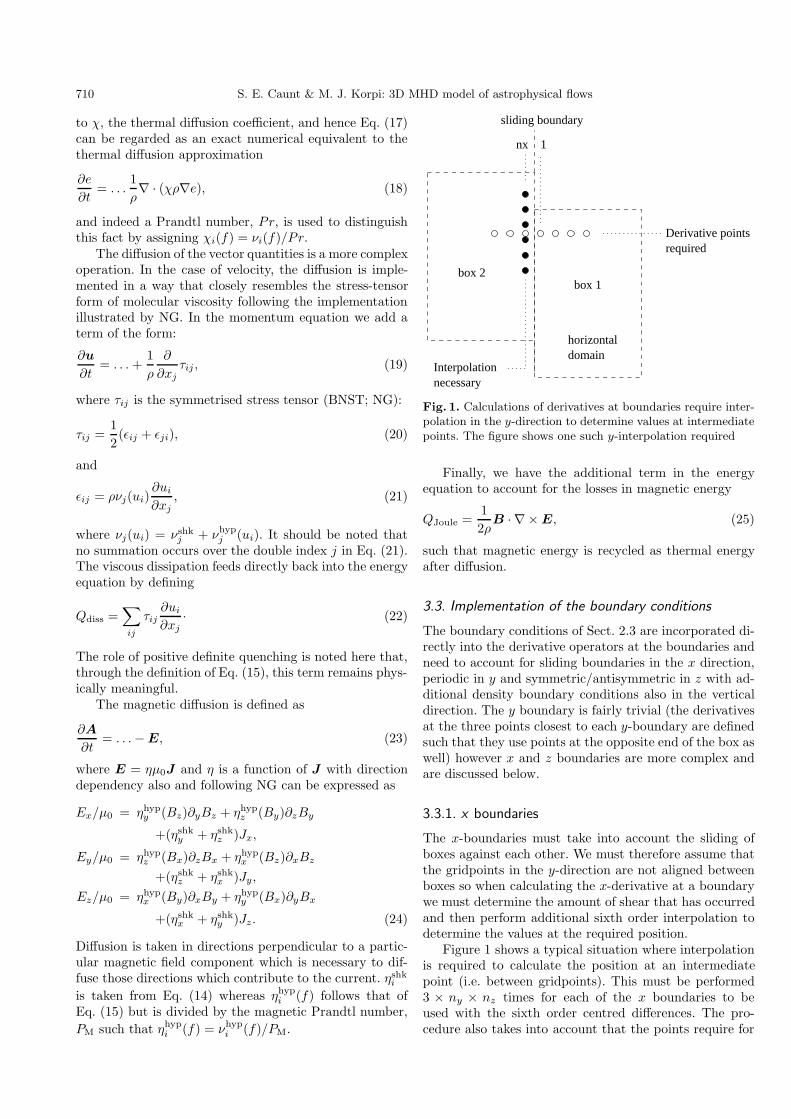
Fig. 1. Calculations of derivatives at boundaries require inter-polation in the y-direction to determine values at intermediatepoints. The figure shows one such y-interpolation required

Finally, we have the additional term in the energyequation to account for the losses in magnetic energy

QJoule =12ρB · ∇ ×E, (25)

such that magnetic energy is recycled as thermal energyafter diffusion.

3.3. Implementation of the boundary conditions

The boundary conditions of Sect. 2.3 are incorporated di-rectly into the derivative operators at the boundaries andneed to account for sliding boundaries in the x direction,periodic in y and symmetric/antisymmetric in z with ad-ditional density boundary conditions also in the verticaldirection. The y boundary is fairly trivial (the derivativesat the three points closest to each y-boundary are definedsuch that they use points at the opposite end of the box aswell) however x and z boundaries are more complex andare discussed below.

3.3.1. x boundaries

The x-boundaries must take into account the sliding ofboxes against each other. We must therefore assume thatthe gridpoints in the y-direction are not aligned betweenboxes so when calculating the x-derivative at a boundarywe must determine the amount of shear that has occurredand then perform additional sixth order interpolation todetermine the values at the required position.

Figure 1 shows a typical situation where interpolationis required to calculate the position at an intermediatepoint (i.e. between gridpoints). This must be performed3 × ny × nz times for each of the x boundaries to beused with the sixth order centred differences. The pro-cedure also takes into account that the points require for


z boundary

antisymmetric function

f(z)

z boundary

symmetric function

f(z)

f=0

Fig. 2. Calculations of derivatives at vertical boundaries canbe performed by specifying the function to be symmetric or

antisymmetric to produce∂fzbc∂z = 0 and fzbc = 0 respectively

a particular interpolation may lie in adjacent boxes in they-direction.

3.3.2. z boundaries

For the velocity, magnetic vector potential and energy wedesire that either the function value is equal to zero orthe first derivative in the z direction is zero. These can beimplemented using symmetric and antisymmetric bound-ary conditions, respectively, to mimic points outside thenumerical domain as described by NG.

Figure 2 shows that by specifying the points outsidethe boundary such that, if we assume that the index of theboundary grid point is b, then for a symmetric boundarycondition

fb−i = fb+i i = 1...3, (26)

results in a calculation that specifies ∂fzbc∂z = 0. Similarly

for an antisymmetric boundary condition of specifyingthat

fb−i = −fb+i i = 1...3, (27)

results in effectively setting fzbc = 0.The density boundaries are calculated from the hydro-

static equilibrium condition Eq. (11) by setting

ln ρb+i = ln ρb−i + 2i∆zg

(γ − 1)eb· (28)

3.4. Calculation of the time-step

The time-step is limited by the Courant-Friedrichs-Lewycondition

∆t ≤ ∆tc =∆x

|u|+ cs + va + |ui=10 | , (29)

where ∆x is set to be the minimum mesh size over thethree directions, va = (|B|2/ρ)1/2 is the Alfven speed,ui=1

0 is the velocity of the underlying shear flow, andcs = (γp/ρ)1/2 is the sound speed. This essentially statesthat information must only be advanced a fraction of themesh size for each time-step. To guarantee the numerical

stability, we choose a safety factor cc ≤ 1 (usually 0.3–0.5)so that the estimated Courant time-step is

∆t = cc∆tc. (30)

We also take into account diffusion when calculating thetime step. Stronger diffusion results in smaller time-stepsand we take into account the hyperdiffusion, shock viscos-ity and magnetic shock dissipation. This condition can beexpressed as

∆td =cd∆x2

max(ν, η)(31)

for which both the shock and hyperdiffusive quantities ofν and χ are included and where cd is an additional safetyfactor, taken from empirical estimates to be of the orderof 0.05.

A radiative time-scale is included by taking the ther-mal conduction as the relevant quantity. Taking a similarform the the above expression we express this as

∆tr =cr∆x2

χshk + χhyp, (32)

again using maximum values for χ and a safety factor ofcr = 0.05.

The final time-step is then derived from the minimumvalue of these three time-scales and we find that this isadequate to ensure that the code remains stable in allconditions.

3.5. Comparison of time-stepping schemes

As mentioned earlier, we use an Adams-Bashforth-Moulton third order predictor corrector scheme to advancethe equations in time. We have tested the performance ofthis compared a number of different methods and foundthat it behaves favourably compared to them.

We have used the standard one-dimensional shock tubetest (described in more detail in Sect. 5.1) as a check on theaccuracy of the scheme since an exact analytical solutionto this problem can be found. This has been chosen as anadequate method of determining the accuracy of a combi-nation of different elements of the code (namely the differ-encing operators in conjunction with the time stepping).For reliable test results the resolution of the numerical do-main is varied and the time-step adjusted accordingly tomore realistically match the resolution (but fixed for theduration of the test). In other words when the resolutionis doubled, the time-step is halved.

From the initial condition, the equations are advancedusing a constant time-step to a time of t = 0.256. Theerror between the true (analytical) and numerical resultsis calculated as a sum for density, velocity and energy andaveraged over the total number of gridpoints. Hence theerror, ε, is given by

ε =Σi(ρ− ρi) + Σi(u− ui) + Σi(e− ei)

nx, (33)


where the quantities with subscript i are the numericalvalues and those without are the analytical values and nxis the number of gridpoints.

As well as the third order Adams-Bashforth-Moultonmethod we have performed the test on the second orderAdams-Bashforth-Moulton method, second and fourth or-der Runge-Kutta methods and the third order predictor-corrector method of Hyman (Hyman 1979).

Fig. 3. Errors incurred by the different schemes for the Sodtube test using different resolutions and time-step sizes

The results of this test are shown in Fig. 3. Here wesee very clearly that as the resolution is increased andthe time-step shortened the higher order schemes producesmaller errors and in all cases the errors from the Adams-Bashforth-Moulton third order scheme are the smallest.It is for this reason that we have chosen this method ofadvancing the equations. The exact algorithm used for thisscheme is given in Appendix B.

4. Parallelisation

4.1. Methods

We chose to use High Performance Fortran (HPF) dueto its simplicity of implementing parallelisation methodsand being ideally suited to data parallelisation. The finitedifference model itself is ideal for running on a numberof processors supporting the Single Instruction MultipleData (SIMD) programming style where data is distributedonto the local memory of each processor. The operationsat a particular grid-point are highly localised with datafrom only three nearest-neighbour points being involvedin any particular operation. This results in a situation inwhich the data can be split between a large number ofprocessors, with communication between processors onlyoccurring at their common data boundaries. Hence, the ef-ficiency of the parallelisation should theoretically improvefor large data sets for which the boundary region size be-comes small in comparison to the size of the inner dataregion on a particular processor (this fact is illustrated

from the tests shown later in this section). In effect, thedata set on each processor can be operated on virtuallyindependently of all the other processors.

HPF directs the processor to distribute and align allthe data variables over a number of processors, effec-tively splitting the domain into a number of smaller sub-domains. The communication calls are automatically de-termined by the compiler. This provides a particularlyflexible approach to parallelisation since it can be eas-ily altered to match the relative number of gridpoints indifferent dimensions.

4.2. Parallelisation tests

Many test have been performed to produce the most op-timal parallelisation results. Most of the tests have beenperformed on the Cray T3E supercomputer at the Centrefor Scientific Computing (CSC) in Espoo, Finland. Theseinclude coding of derivative routines, calculations of theshearing boundary conditions, ghostzone boundaries andcalculations of array operations. However, the most strik-ing results were determined for how best to distribute thedata over a number of processors. In theory the best dis-tribution occurs for the smallest surface area of bound-aries between processors since communication is at a min-imum in this situation. However, our timings indicatethat this is not necessarily the best option with timingswidely varying between different distributions for the samecalculations.

To test the effectiveness of the different options avail-able for distributing data (one-dimensional slabs, two-dimensional columns or three-dimensional blocks as illus-trated in Fig. 4) we use a simple test code that calculatesderivatives 1000 times in all three directions (assumingperiodic boundaries) using a block of data of equal di-mensions (63 × 63 × 63). This data is distributed over8 processors chosen as it allows the processors to be ar-ranged in a cube when distributed in three dimensions forwhich the communication should be minimised. Resultsfor this test are given in Table 1 and shown in Fig. 5 forthe total times taken of all three derivatives. Followingthe notation of HPF directives, distribution over a partic-ular dimension is labeled as “B” for “BLOCK” (data isdistributed as a block onto a particular processor in thisdirection) and “*” if distribution does not occur along thisparticular direction.

From these tests we see that distributing in the x direc-tion performs very poorly either alone or when distributedalong with others. It was also observed that speed up ofcodes in general is bad when data is distributed along thisdirection. This is probably related to the Fortran columnmajor ordering of arrays (i.e. “first index changes fastest”)in memory which can lead to caching problems.

The y and z distributions perform well and it is seenthat the distribution over both of these directions togetherperforms the best overall. This is presumably because thedecreased surface area of the boundaries between data


Block distribution Block distribution Block distributionin three dimensionsin two dimensionsin one dimension

Fig. 4. Data distribution over different numbers of dimensions. From left to right these are one-dimensional, or slab distribution,two-dimensional or column distribution and three-dimensional or block distribution

Table 1. Comparisons of times of each derivative routine whenvarying the distribution scheme. The total time taken for allthree routines is shown and this is plotted in Fig. 5

Distribution x-der. y-der. z-der. total

(B, *, *) 194.52 49.65 49.52 293.69(*, B, *) 26.62 9.64 27.53 66.79(*, *, B) 29.34 27.56 13.69 70.59(B, B, *) 51.93 98.05 36.47 186.45(B, *, B) 52.04 33.41 105.40 190.85(*, B, B) 29.70 6.42 10.13 46.25(B, B, B) 52.45 52.02 54.39 158.86

Fig. 5. Comparisons of times to perform parallel calculationswhen data is distributed over different directions. All distri-butions where parallelisation has occurred over the x-directionshow dramatically decreased performance

distributed on the processors has lead to less communi-cation. This is seen by comparing the y-derivative timingfor the (*, B, *) distribution and the z-derivative timingfor the (*, *, B) with the same for the (*, B, B) distributionin Table 1 in which both times are seen to decrease whendata has been spread more evenly in different directions.

2

3

4

1

2

3

4

boundary communication for x−boundary of processor 1

1

Fig. 6. Communication required for shearing boundaries whendistribution occurs in the y-direction. In general, the pointsrequired across the x-boundary for one particular processorare not aligned on the same processor and are typically storedin two processors located at any position within the computer

4.3. Shearing boundaries

When incorporating shearing boundaries the results fordistributing data along the y-direction is less efficient sincegridpoints at one point on one side of the box in generalneed to communicate with points at a totally different lo-cation on the other side of the box as shown in the exampleof Fig. 6 where data has been distributed over 4 processorsin the y-direction.

Here we see that due to the shearing, the calculationsat one of the x-boundaries on processors 1 require commu-nication to acquire data on processors 3 and 4. In generalit could be any of the processors. This is obviously muchmore expensive and complex than simply communicatingwith points directly opposite the boundary. This in effectresults in poorer performance when data is distributed inthis direction because communication does not necessarilytake place between neighbouring processors.


Typical galacticbox appearance

x

z

y

box appearanceTypical accretion disk Typical stellar

box appearance

Fig. 7. Different box dimensions for different applications of the code. Each performs better under different parallel distributionsrelated to the grid dimensions. For example the galactic box performs more efficiently for distribution in the z-dimension dueto the grid resolution being weighted in this direction

4.4. Performance of the full code

From the above tests we see that the best performanceof the parallel code can be achieved by distributing dataalong the y and z directions.

We also need to take into account the different modeldimensions that are likely to be used when determiningwhich distribution method to use. We therefore perform anumber of tests on the speed up of the code for differentdimension models and different distributions.

We chose to determine the speed up of the code bycomparing timings of the code when doubling the resolu-tion and doubling the number of processors. In an ideallyparallelised code the real time of communication shouldremain constant (however boundary conditions will effectresults). We also use this method rather than keeping afixed resolution and comparing timings when doubling thenumber of processors due to the limiting fact that theCray T3E contains only 128Mb of RAM of local memoryon each processor. This implies naturally that high reso-lution simulations can only be run on a large number ofprocessors and hence trends in speed-up are impossible totest. The other alternative with this method is to use alow resolution simulation that will run on a small num-ber of processors. However, this is an artificial test for tworeasons: firstly the main aim is to run high resolution sim-ulations and secondly when distributed over a large num-ber of processors, communication time becomes artificiallyhigh since only a small number of gridpoints in a particu-lar direction lie on a given processor. This test is designedto illustrate the essential reasons behind parallelising thecode; namely that through parallelisation, high resolutionsimulations can be performed in appreciable times.

The test uses all parts of the code including magneticterms, shearing and numerical diffusion. The test is notaimed at solving a physical problem but the data is ini-tialised as it could be for a typical galactic run with a large

scale azimuthal magnetic field. The code is then timed forperforming 30 time-steps.

Three tests are displayed here showing the results fordifferent distributions of data corresponding to differentshapes of boxes that are commonly used in different as-trophysical systems as shown in Fig. 7. For the galacticsetup, distribution in the z-direction results in the bestdistribution of data amongst processors while for the ac-cretion disk and stellar applications, y and y-z distribu-tions are best. Hence grid resolutions and distributions ofdata are chosen to match each of these situations as closelyas possibly. For all the tests performed we have roughlyan equal number of gridpoints per processor making com-parisons between distributions possible also.

For ideal parallelisation, the real time of calculationshould remain constant when doubling the number of pro-cessors and doubling the grid resolution. We thereforemeasure performance on real time per grid-point. Theseare then scaled as a percentage of the time taken on twoprocessors.

Table 2 shows the times for distributing the data inthe vertical direction for a grid resolution that is biasedtowards the vertical. Figure 8 shows plots of the relativetimes and speed up of the code. Tables 3 and 4 along withFigs. 9 and 10 respectively show the results for the alter-native types of box dimensions and data distributions.

We see that out of the three tests, the times for the ver-tical distribution are the best. This is because the shearingboundaries are not affected by the parallelisation. Datathat is required by one particular point on an x-boundaryalways lies on the same processor therefore expensive com-munication does not occur. We also note, that in general,as the number of processors increases (along with the gridresolution), the performance appears to improve which isseen from the graphs where the speed up is above optimal.This is due to the percentage of time taken up in calcu-lating the boundary conditions diminishing as the overallsize of the model increases. All the results show that the


Table 2. Times for distributing the data (*, *, BLOCK) typ-ical for a galactic simulation

No. of Grid Real time Relativeprocs. resolution (s) speed up

2 31× 31× 255 742.61 2.004 31× 63× 255 764.51 3.958 63× 63× 255 711.29 8.6216 63× 63× 511 708.45 17.4032 63× 127× 511 738.99 33.5664 127× 127× 511 734.29 68.26128 127× 127× 1023 732.26 136.99

Table 3. Times for distributing the data (*, BLOCK, *) typ-ical for an accretion disk simulation


2 31× 255× 31 879.23 2.004 31× 255× 63 905.84 3.948 63× 255× 63 808.41 8.9716 63× 511× 63 802.86 18.1832 63× 511× 127 862.69 34.0164 127× 511× 127 870.33 68.03128 127× 1023× 127 898.92 131.58

Table 4. Times for distributing the data (*, BLOCK, BLOCK)typical for a stellar simulation


2 63× 63× 63 811.98 2.004 63× 63× 127 824.25 3.968 63× 127× 127 827.86 7.9616 127× 127× 127 772.57 17.2432 127× 127× 255 778.36 34.3064 127× 255× 255 796.55 68.5128 255× 255× 255 792.46 136.02

code has good speed up when doubling the resolution anddoubling the number of processors with virtually linearspeed up in all cases.

5. Tests

The code has been tested against a number of standard hy-drodynamical and magneto-hydrodynamical tests in 1D,2D and 3D. These tests have been designed to test individ-ual properties of the code as well as all components of thecode working together. Some of these tests are “standard”tests of fluid models and others have been incorporated tocompare the results of our method against the existinganalytical solutions and other numerical models.

Most of the hydrodynamical tests are designed to de-termine the effectiveness of the numerical viscosities instabilising the code, removing unphysical features andcapturing the essential physics of a particular problem.They are also aimed at determining the ability of the

Fig. 8. Performance of the code starting from 31 × 31 × 255to 127 × 127 × 1023 from 2 to 128 processors distributing thedata as (*, *, BLOCK). See Table 2 for intermediate sizes andactual timings

Fig. 9. Performance of the code starting from 31 × 255 × 31to 127 × 1023 × 127 from 2 to 128 processors distributing thedata as (*, BLOCK, *). See Table 3 for intermediate sizes andactual timings

Fig. 10. Performance of the code starting from 63×63×63 to255× 255× 255 from 2 to 128 processors distributing the dataas (*, BLOCK, BLOCK). See Table 4 for intermediate sizesand actual timings


Fig. 11. Results for the weak Riemann shock-tube test where the density on the left is initially set to ρ = 1.0 at t = 0.245 for255 gridpoints. Figures plotted are for density, pressure, velocity and energy. The dashed line shows the analytical solution

Cartesian grid to reproduce spherical features. For all testswe use cshk = 2.0 and chyp = 0.05 for the coefficients ofthe shock and hyperviscosities. The Prandtl number andmagnetic Prandtl numbers are equally set to unity.

Using the MHD test suite of Stone et al. (1992) andStone & Norman (1992b) as a basis for the magneto-hydrodynamic tests, we perform a number of identicaltests again using previously published results for compar-ison with our numerical method. These tests are designedto examine the stability of the fluid and magnetic fieldevolution and more specifically to check that the char-acteristics of the MHD flow are correct, specifically thepropagation of MHD waves.

These tests have allowed us to determine the effec-tiveness of the algorithms used, as well as to show theirweaknesses. All tests have been performed using resolu-tions comparable to those expected in “real” simulationsand hence act as a gauge on the accuracy one can expectfrom future calculations.

5.1. Riemann shock tube test

The Riemann shock tube test (Sod 1978) has been usedby many authors as a test of numerical algorithms. All

components of the hydrodynamical code are used includ-ing numerical viscosities. This test determines the abilityof the code to capture shocks, formed from discontinuitiesin the fluid properties, and therefore it particularly is adirect test of the shock viscosity employed.

Starting from an initial discontinuity in the densityand energy, the fluid forms a shock front and a rarefrac-tion wave. For this test an exact analytical solution can befound (e.g. Hawley et al. 1984), which provides an ideal sit-uation for determining the accuracy of the code includingthe propagation speed of the waves, the jump conditionsat the shock front, and the ability of the code in stabilisingdiscontinuities within the fluid.

We perform two test cases; one using the standardsetup described by Sod (1978) and another for which theshock is much stronger. This second test is included as amore accurate measure of the ability of the code to copewith more violent physical features, and as a more extremetest of the numerics.

Both tests are calculated in one dimension (we use thez-dimension with closed boundaries) with a resolution ofnz = 255 with z = 0, 1. The gas has a ratio of specificheats of γ = 1.4 with zero initial velocity. The densityand energy, and therefore pressure, are discontinuous atz = 0.5. For the weak (standard) shock tube test, we have


Fig. 12. Results for the strong Riemann shock-tube test where the density on the left is initially set to ρ = 10.0 at t = 0.150for 255 gridpoints. Figures plotted are the natural logarithm of density, pressure, velocity and energy. The analytical solutionis plotted as a dashed line

on the left ρl = 1.0 and with the strong shock tube testthis is ρl = 10.0. All other variables are the same for thetwo tests with Pl = 1.0, ρr = 0.125 and Pr = 0.1.

Figure 11 shows the evolution of the variables for theweak shock at t = 0.245 compared to the analytical solu-tion, shown as a dashed line. Many features of the fluidproperties have been captured well by the calculation. Theposition of the shock front, the contact discontinuity andthe rarefraction wave are all correct and the magnitudesof the fluid properties in each region is correct. The maindeviations from the analytical curve occur at the contactdiscontinuity and the shock front. At the shock front theshock is captured well within four gridpoints however aslight under-shoot occurs for the energy which is quicklycorrected within three gridpoints. The model has not suc-cessfully reproduced the shape of the contact discontinuityfor energy or density, with both variables being smoothed.This feature appears to be common amongst many dif-ferent numerical schemes as shown in the figures by Sod(1978) and Stone & Norman (1992a). The discontinuitiesin the gradient of the rarefraction wave have been cap-tured well by the scheme, although some smoothing isinevitable.

Figure 12 shows the equivalent variables at t = 0.150for the strong initial discontinuity, with density plottedas a natural logarithm. This, being a more rigorous testof the numerics, shows more unphysical features than theweak shock. However, the different regions of the flow arevery clear and follow well from the true values – the maindifference being the ability of the code to retain the strongshock features. The positions of the boundaries betweenthe different regions all agree very well to the analyticalsolution, however it is noted that the shock front appearsto have moved fractionally further. Small scale oscillationsin the velocity are seen to be generated behind the shock,which is natural of a scheme of this type, however, the hy-perdiffusion has minimised the magnitude of these. Again,the contact discontinuity is smeared by the simulation,and the plateau of maximum energy is not resolved, butdoes not deviate far from the true value. The shock frontitself is still well resolved and retains the essential physicalcharacteristics showing that the shock viscosity is imple-mented correctly. In this case, the under-shoot is smallerthan for the weak shock. The rarefraction wave still clearlyremains close to the analytical solution and the discontinu-ous gradients are well represented. Considering the stronginitial conditions presented to the flow, we feel that the


numerical solution presents a good fit to the analyticalone.

5.2. Blast waves

The next set of tests is aimed at testing the capabilityof the code to model spherical features with a Cartesiangrid. We perform three 3D tests of strong blast waves:adiabatic, radiative, and with a strong imposed magneticfield.

First we follow the evolution of an adiabatic shock cre-ated by an instant injection of purely thermal energy, mon-itoring its shape, radius and expansion velocity, and com-paring it to the analytical Sedov-Taylor solution (Taylor1950; Sedov 1959). The explosion is initialised by adding1051 ergs of thermal energy, roughly corresponding to arealistic SN explosion (e.g. Heiles 1987), in a single grid-point in the middle of the computational volume sized1 kpc3. The number of gridpoints used in the test is 1273.The surrounding ISM has a uniform density of 1.0 cm−3

and temperature 104 K without any magnetic field. Noheating or cooling terms are applied to the energy Eq. (4).According to the Sedov-Taylor solution, based on similar-ity analysis, the shock front produced by a strong explo-sion in a uniform medium (in a three-dimensional volume)moves through it so that its radius as function of time is

R(t) = Eρ02/5t1/5, (34)

where E is the explosion energy and ρ0 is the density ofthe surrounding ISM. Firstly we compare the expansionof the simulated blastwave to the Sedov-Taylor solutionby plotting its radius versus time in a logarithmic scalein Fig. 14. If the blastwave is to follow the Sedov-Taylorsolution, there should be a powerlaw with the slope 2/5visible in this figure, and in addition the simulated ra-dius should fall on top of the dashed line representing theSedov-Taylor solution for the selected E and ρ0. Initiallythe blastwave is observed to expand faster than the Sedov-Taylor theory predicts, which is due the free expansionphase during which the explosion front has not yet sweptup enough mass to form a shock front and therefore ex-pands freely. In reality SN explosions, and also the free-expansion phase, occur at much smaller scales than thegrid resolution of numerical models, so the “late” free ex-pansion phase observed here is an artifact from the finiteresolution. After the first few tens of thousands of years ofevolution, when the shock has formed, the remnant startsfollowing the Sedov solution rather closely, and only after4 million years the expansion starts slightly deviating fromthat powerlaw. At that point the expansion velocity of theremnant has become comparable to the local sound speed,when the shock dies out, and the remnant starts dissolvingto the surrounding ISM. The previously thin shock frontforms a thicker shell, and matter is flowing in and out asthe shell relaxes. In Fig. 13 we also show the shape of theblast wave in the horizontal (xy) plane, and the 1D pro-files of density and velocity on top of the ones calculated

Table 5. The cooling function used for investigating radiativeblastwaves

Ti [K] Λi [erg s−1 g−2 cm3] βi

100 1.14 1015 2.000

2000 5.08 1016 1.500

8000 2.35 1011 2.867

105 9.03 1028 −0.650

from the Sedov-Taylor solution. Throughout the calcula-tion the blast wave remains spherical as can be seen fromthe left panel of Fig. 13, which shows the remnant at laterstages (22 Myrs). During the shock stage the profiles ofthe physical quantities resemble quite well the analyticalprofiles, although the jump conditions are not quite satis-fied at the shock front (on the right in Fig. 13).

The Sedov solution serves as a good approximationfor a SN explosion when the radiative losses are negligible,which is true roughly during the first 105 years of its evolu-tion (e.g. Shu 1992). When the radiative losses become sig-nificant, they change the expansion characteristics of theremnant, as discussed e.g. by Ostriker & McKee (1988).We investigate a radiative remnant with the same setup asused for the adiabatic case, but adopting a cooling func-tion derived by Dalgarno & McCray (1972) and Raymondet al. (1976) that has been previously used in several ISMmodels (e.g. Rosen & Bregman 1995; Vazquez-Semadeniet al. 1995), which is implemented as a sink term in theenergy Eq. (4) so that

∂e

∂t= . . .− ρΛ, (35)

where Λ = ΛiT βi, Ti ≤ T ≤ Ti+1, is the piece-wise coolingfunction described in Table 5. The position of the radia-tive shock front is shown in Fig. 14, whereby it can beseen that during the first tens of thousands of years theexpansion of the blast wave follows rather closely to theadiabatic case, but after approximately 105 years the twoexpansion curves start deviating from each other, indi-cating that the radiative losses have become significant.After that time the remnant shows powerlaw expansionas in the adiabatic case, but the slope of the line is con-siderably less, about 0.29, which is close to the slope 1/4reported in Ostriker & McKee (1988) for a radiative blast-wave in homogeneous medium. Due to the energy loss viaradiation, the expansion velocity drops much faster thanin the adiabatic case, being comparable to the sound speedalready at one million years.

Finally, we investigate adiabatic blast waves in thepresence of a strong azimuthal magnetic field. The setupis identical to the adiabatic case, but now we impose anazimuthal magnetic field of the strength 5 µG at eachtime-step, and follow the position of the blast wave in thedirection along the field lines (y-direction), and perpen-dicular to them (x-direction), which curves are shown inFig. 14. The shape of the blast wave is shown as density


Fig. 13. Lefthand panel shows spherically symmetric expansion of an adiabatic blast wave, showing grey-scale representation oflogarithmic density at the horizontal mid-plane of a 3D simulation using 1273 gridpoints at 22 Myrs. On the right we show the1D profiles of density and velocity during the shock stage at 3 Myrs for the resolution 255 plotted on the analytical Sedov-Taylorsolution

Fig. 14. Position of the expanding remnants for different setups. The leftmost panel shows the expansion of adiabatic andradiative remnants in three dimensions. The panel on the right shows the expansion of adiabatic remnant in a uniform azimuthalmagnetic field. The dashed line in both figures shows the Sedov-Taylor expansion law with the slope 0.4. For the magnetic casethe expansion of the remnant in the azimuthal direction is shown with a solid line, while in the x-direction it is dot-dashed.The magneto-sonic wave moving in the x-direction is represented by the dotted line

contours over-plotted with velocity field vectors at the hor-izontal mid-plane in the left-hand panel of Fig. 15. In theright-hand side of Fig. 15 we show a voxel projection of the3D density field with perturbed magnetic field lines. Allthese figures illustrate how the magnetic field can severelyaffect the expansion. Along the magnetic field lines theblast wave expands in a normal fashion and develops astrong shock front. However due to magnetic tension of thefield lines, this does not occur along the x direction. Wealso see formation of a magnetosonic wave, which prop-agates perpendicular to the field lines, forming a weakspherical perturbation, slightly pinched at the poles. Theshape of the perturbation is similar to the one describedby Ferriere et al. (1991). In the x-direction the expansionvelocity of the blast wave is heavily damped, and most of

the expanding motion occurs in the y-direction, as seene.g. in the simulations of Tomisaka 1998). In Fig. 14 theexpansion in the y-direction is seen to roughly follow theSedov-Taylor law, but the x-direction strongly deviatesfrom it. The expansion of the magnetosonic wave is muchfaster than the non-inhibited blast wave, since it is movingwith the Alfven velocity 14 km s−1, which after approxi-mately 4 Myrs becomes faster than the blast wave itself.In three dimensions the spherical blast wave is unrecognis-able. Complex features have been formed, where the mag-netosonic wave has created a lemon-shaped weak densityperturbation within which the blast wave has produced acavity elongated in the y-direction.


Fig. 15. Interaction of blastwave with large-scale azimuthal magnetic field. The lefthand panel shows a 2D slice through thehorizontal midplane with density shown in grey-scale with velocity field plotted on top with arrows. The righthand panel showsthe voxel projection of the density with the perturbed magnetic field lines plotted on top. The expansion of the shock front isseen to be restricted to the azimuthal direction while the magneto-sonic wave perturbs the density in the poloidal directions

5.3. Interacting blast waves

We perform two tests, in one and two dimensions, to showthe ability of the code to deal with interacting blast waves.The first follows the one-dimensional colliding blast wavetest presented by Woodward & Colella (1984) who per-formed this test on various algorithms comparing a veryhigh-resolution case to lower-resolution ones. We performa similar test, comparing a high-resolution calculation toa moderate resolution case. One reason for this test isto compare the high-resolution case to the Woodward &Colella case as a check on shock velocities and density pro-files, and a second reason is to see how the code adaptswith different resolutions. If the code scales well (and inparticular the numerical viscosities) between different res-olutions then one would expect the shock positions andprofiles to be in close agreement.

The test setup follows that of Woodward & Colella(1984). The numerical domain is in the vertical direction,again for reasons of boundary conditions, with z = 0, 1and the ratio of specific heats set to be γ = 1.4. Velocity isinitially at zero with density everywhere set to be ρ = 1.0.Two shock waves are generated by setting two discontinu-ities in the pressure. For z = 0.0, 0.1 we set P = 1000,z = 0.1, 0.9 P = 0.01 and for z = 0.9, 1.0 we haveP = 100, hence two blast waves of different magnitudesare generated moving towards each other.

Since no exact analytical solution exists, we performa very high-resolution test calculation to obtain profileswhich can be considered to be highly accurate. For thiswe set nz = 8191 which allows the sharp density peak atthe time of collision to be well resolved. For the moderateresolution, we set nz = 511.

Figure 16 shows the evolution of the fluid at three dif-ferent times, each of which can be compared to the figuresshown by Woodward & Colella (1984). The very high-resolution calculation is shown as a dashed line with the

moderate resolution plotted on top as diamonds. Evidentfrom all the figures is that the shocks travel at identicalspeeds for both resolutions, an important factor when us-ing the code at different resolutions. One also observesthat the shapes of the curves are almost exactly the same.At t = 0.028 we see a slight deviation in the velocitybehind the shock front, but in all other aspects and atother times the different resolutions appear to be virtu-ally identical. The lower resolution run obviously cannotresolve very small features, and this is evident at the timeof collision when the density spike is smaller, but is in thecorrect position. At the final stage the density minima andmaxima are again smoothed as a consequence of the lowerresolution, but retain the same shape as the very high-resolution case. Overall, we feel that the lower resolutionsimulation compares very well to the high resolution case,and compared to the original Woodward and Colella fig-ures of lower resolution calculations (which are howeverfor 1200 grid zones) performs very well.

The second test we perform is a two-dimensional teston colliding spherical remnants produced by two equallystrong explosions in a uniform medium, which is the con-figuration discussed e.g. by Courant & Friedrichs (1948),and studied also with numerical models e.g. by Yoshioka& Ikeuchi (1990) and Voinovich & Chernin (1995). Weagain initialise the two explosions as thermal energy re-leases in a single grid-point corresponding to a SN en-ergy of 1051 ergs, located 0.4 kpc apart from each other.The remnants collide after 1 Myr, having equal expan-sion velocities, and instantly after the collision a reflectedshock front is formed propagating back into the hot andsparse interiors, as seen in the top left panel of Fig. 17.At the location of collision, a tangential line forms, alongwhich the radial flow stops persisting throughout the sim-ulation, and thereby seen in all the panels of Fig. 17.Soon afterwards a new shock front, denoted as the Machfront by Courant & Friedrichs (1948) traveling along this


Fig. 16. Results for the interacting blastwaves, taken in one-dimension. The points show the resolution of 511 gridpoints andthe solid line is for 8191 gridpoints. Plots of velocity and density are shown at three different times (t = 0.010, t = 0.028 andt = 0.038). The lower resolution case closely follows the evolution of the more accurate high resolution simulation howeverstrong peaks are damped

line appears, with the velocity exceeding the expansionof the unperturbed remnants. This configuration seen inthe simulation at this stage closely resembles the classicalCourant-Friedrichs picture. The top right panel of Fig. 17shows that after about 10 Myrs the Mach front has propa-gated outwards and increased its surface area, so that thewhole systems starts becoming spherical on the outside,even more pronounced in the lower panel at 34 Myrs. At

the same time the curved reflected shock fronts expand inthe hot sparse interior having largest expansion velocitiesin the direction of the smallest density with vortical mo-tions occurring leading to kidney-shaped structures. Theappearance of the flow is in good agreement with other nu-merical simulations, such as the detailed calculation pre-sented by Voinovich & Chernin (1995) and also with theresults of Yoshioka & Ikeuchi (1990).


Fig. 17. The two-dimensional evolution of interacting blastwaves generated from two equally strong point explosions (corre-sponding to a typical SNe of 1051 ergs) in a uniform medium with no magnetic field shown at three different times (t = 5 Myrs,t = 12 Myrs and t = 34 Myrs). The collision occurred at t = 1 Myr. Grey-scale and black contours shows logarithmic densitywith velocity field plotted with white arrows on top. The resolution is fixed at 127 gridpoints per kpc

5.4. Magnetic advection test

We now perform an advection test of a pulse of magneticfield. The test is initialised such that a pulse of magneticfield, which is as close as possible to a square wave, is ad-vected at constant velocity in one direction. This is per-haps the least relevant test for the numerical scheme asit requires that most of the PDEs are disabled. In otherwords, the square pulse has no back-reaction on the fluidin any sense. The test is essentially used here to study thenumerical diffusion of the wave (since numerical diffusionacts all the time and quite strongly where fluid propertiesvary rapidly between gridpoints) ensuring that numericalinstabilities are quenched and that the evolution of thecurrent that is generated at the leading and trailing edgesof the pulse is correct.

The test is performed in one dimension along the ver-tical axis. The use of the z-direction is different to Stone& Norman (1992b) and arises from the fact that boundaryconditions in the vertical direction mean that setting uptests such as this (and subsequent tests shown below) issimplified. Discontinuous values of the magnetic vector po-tential in periodic directions result in propagation of waves

from the boundaries. This change in direction also resultsin the use of Bx which in effect means that the test shouldbe otherwise identical. However, the use of the magneticvector potential causes a number of difficulties when ini-tialising the wave and obtaining a perfect square wave isimpossible since discontinuities in the magnetic vector po-tential lead to ringing occurring at the corners of the wave.We therefore start the test from a wave in which the edgesof the pulse are spread over three grid-zones rather thanjust one, which is already slightly smoother than that ofStone & Norman. However we as closely as possible fol-low their setup. The total width of the pulse is over 54gridpoints, with the upper values covering 48. The initialshape of the field and current is shown in the upper panelsof Fig. 18. The pulse is then advected over 250 gridpointsfor which ∆z = 1 with a velocity of uz = 1.

The final state of the advected magnetic field andcurrent is shown in lower two panels of Fig. 18. As ex-pected from the use of the diffusive elements of the model,the edge of the pulse has now been smeared from theinitial three grid-zones to approximately 10. The cur-rent density is therefore similarly smeared. As quoted byStone & Norman, the use of the vector potential can lead


Fig. 18. Advection of pulse of magnetic field in the z direction. The upper two panels show the inital condition of the test withthe left plot showing the radial magnetic field and on the right the azimuthal current density. The deviation from a square waveis due to the use of the magnetic potential. The final state is shown in the lower two panels The resolution is nz = 255 and fora perfect initially square pulse, the edges would be located at z = 255 and z = 305

to the production of non-monotonic currents. Indeed, it isseen that the trailing edges are non-monotonic. However,no sign reversal is seen and the deviations from mono-tonicity are very small in comparison to the maxima ofthe current.

5.5. Propagation of shear Alfven waves

The next test we perform is to propagate Alfven waves ini-tially generated from a shear flow. The test is again set upidentically to that of Stone & Norman (1992b) except forthe use of the z direction again for reasons stated above.

The test is intialised by threading the fluid with a ver-tical magnetic field, Bz, and a small perturbation to uy isadded to a small region of the width one, the extent of thedomain being 15. In terms of dimensionless units, ρ = 1,Bz = 1 and uy = 0.001 in the perturbed region. As withStone & Norman, two tests are performed: one for whichuz = 0 and the perturbed velocity is between the regionsof z = 1 and z = 2 and one for uz = 1.5 with the pertur-bation occurring between z = 2 and z = 3. The shearingmotion then generates square Alfven waves propagating atan Alfven velocity of vA = ±1 (with µ0 = 1). For the firstcase of this test, these propagate with and equal velocity

in each direction (u = ±1) and for the second case onehas an overall velocity of u = uz + vA = 2.5 and the otheru = uz − vA = 0.5. Both calculations have a resolution ofnz = 255.

Figure 19 shows the final state of the azimuthal veloc-ity, uy, and sheared magnetic field, By, for the two cases.For the first case the plots are shown after t = 0.8. Thewaves have clearly traveled the correct distance of z = 0.8corresponding to u = 1 and have propagate evenly in bothdirections away from the initial sheared region. The secondfigure is shown after a time of t = 1.0, when the two waveshave traveled distances of z = 2.5 and z = 0.5 correspond-ing to the right and left waves respectively. Again thesecorrespond correctly to the overall velocities of u = 2.5and u = 0.5. Also, the widths of the square pulses arealmost identical to the initial width of the sheared regionin both cases.

It can be seen that in the second case the diffusion hasacted more strongly. This is due to the magnitude of thehyperdiffusion depending upon both Alfven velocity andfluid velocity and hence being greater for the case in whichuz = 1.5.


Fig. 19. Propagation of shear Alfven wave in a fluid threaded by a vertical magnetic field. The upper panel is for an initiallystationary fluid and the lower for a fluid with initial velocity of uz = 1.5. For the stationary fluid, the wave is generated by aperturbation in velocity that was initially located between z = 1 and z = 2 whereas for the non-stationary case it is locatedbetween z = 2 and z = 3. Both cases show that square pulses of magnetic field are generated, propagating perpendicular to theapplied magnetic field at the correct velocity. The resolution is set to nz = 255

5.6. Magnetic braking of an aligned rotator

The third test is the magnetic braking of an aligned rota-tor. This is virtually identical to the previous test in whichthe fluid is threaded by a magnetic field and a region ofthe fluid is then perturbed azimuthally. For this test how-ever, there is a density contrast between the perturbedregion and the steady region resulting in a setup whichmimics a disk of high density surrounded by a low densitymedium. The perturbation generates Alfven waves prop-agating away from the disk and also into the disk thusaccelerating the fluid in the surrounding medium and de-celerating the disk. Subsequent partial reflections from thesurface of the disk further complicate the system, eachbeing both transmitted as a lower amplitude waves intothe medium and back into the disk. A more comprehen-sive discussion of the model is given by Stone & Norman(1992b).

Again, using identical parameters to Stone & Norman,the disk is of density ρd = 10.0 and the surroundingmedium is of ρm = 1.0. The test again is in the z-directionwith 300 grid-zones. The disk is located in the regionz < 1 and the low density medium extends from this pointto z = 15. The vertical magnetic field has a strength of

Bz = 1. Setting uy = 0.001 in the region z < 1 and zeroelsewhere, we are able to make comparisons to the ana-lytical results of Mouschovias & Paleologou (1980). Theprofiles of the resulting sheared magnetic field, By, andazimuthal velocity, uy, are independent of the initial ve-locity (varying only in magnitude).

Figure 20 shows the final state of the relevant quan-tities after t = 13. The dashed line shows the analyticalvalues for comparison. The waves, which are generatedfrom the initial shear and subsequent reflections at thedisk surface, closely match the profiles of the analyticalvalues but are smoothed due to the inherent diffusion ofthe scheme. However, propagation speed and magnitudesare correct.

5.7. MHD Riemann shock tube test

The next test is the MHD equivalent to the Riemann shocktube test (Sod 1978) . This has been discussed in detail fora number of numerical schemes by Brio & Wu (1988) andused as a subsequent test by Stone & Norman (1992b).This tests uses all elements of the code to evolve a fluidthat is initiated with a discontinuous pressure and mag-netic field at the midpoint with an additional component


Fig. 20. Results of the magnetically braked aligned rotator showing the resulting azimuthal velocity and magnetic field att = 13. The fluid is threaded by a vertical magnetic field and the fluid density remains fixed with ρ = 10 between z = 0 andz = 1 and ρ = 1.0 for the remaining domain. The high density region is initially given a perturbing azimuthal velocity whichgenerates Alfven waves moving both inwards and outwards. The dashed line shows the analytical solution. The resolution is setto 301 gridpoints

of the magnetic field along the direction of motion. Unlikethe standard shock tube test, no known analytical solutionexists for the subsequent evolution of the fluid and mag-netic field. Hence we make comparisons to the previouslypublished works mentioned above.

The hydrodynamical parts of the test are initialisedexactly as in the hydrodynamical counterpart. The do-main size of the problem is however larger (800 grid-zoneswith ∆z = 1 to match the published results of Brio & Wu(1988) and Stone & Norman (1992b). We again use the zdirection due to the boundary conditions and change thedirection of the discontinuous magnetic field accordingly.The discontinuity is at the centre of the domain. Fluid tothe left takes physical values of ρl = 1.0, Pl = 1.0 and(Bx)l = 1.0. and to the right takes ρr = 0.1, Pr = 0.1 and(Bx)r = −1.0. An additional magnetic field of Bz = 0.75is constant throughout the domain. As in the previouslypublished MHD Riemann shock tube tests, we take γ = 2.As with the magnetic advection test, the use of the mag-netic vector potential produces problems when setting updiscontinuous magnetic fields. The initial discontinuity istherefore spread over three grid-zones. However we feelthat, with the use of magnetic shock viscosities and hyper-diffusion, this small initial difference has negligible effectson the resulting evolution.

Unlike the hydrodynamical case, the MHD shock tubetest generates many kinds of waves as well as the shockand rarefraction wave. As quoted by Brio & Wu, the fluidcan contain a compound wave which consists of a shockwave attached to a rarefraction wave of the same family.As seen by the results in Fig. 21, this complexity is clearlyevident.

Figure 21 shows the final state of the fluid and mag-netic field at t = 80. All waves shown in the results of Brio& Wu are evident, including the left moving fast rarefrac-tion wave, slow shock and rarefraction wave compound,right moving contact discontinuity, slow shock and fast

rarefraction wave. Comparisons also show that they havemoved with the correct velocities and magnitudes, and arein close agreement with the published results of Brio & Wu(1988) and Stone & Norman (1992b).

6. Summary

In this paper we have described a numerical model for sim-ulating magnetised shear-flows in astrophysical systemssuch as galaxies or accretions disks. Starting from the ba-sic non-ideal MHD equations describing the fluid, we havediscussed their numerical implementation on the standardshearing box model. Using explicit finite-difference calcu-lations, fluid properties are discretised onto a regular meshin three dimensions. The fluid is advanced through timeusing a third order accurate predictor-corrector scheme,which has been shown to compare favourably to other ad-vancing schemes.

An important feature of the model comes from thediffusion methods, which are implemented for two reasons,firstly to resolve and model discontinuities in the flow,and secondly to stabilize the numerics. The method workswell as introducing diffusion only in the necessary regionsleaving well resolved regions of the fluid unaffected.

An important aim of this work is to perform high res-olution calculations and as a result the model has beendesigned to take advantage of parallel computers. We havetherefore illustrated the methods we have invoked to par-allelise the code and shown their performance. Similarlyimportant feature of the model is to make it easily adapt-able to incorporate new physics or numerical techniques.The parallelisation method adopted, namely HPF, hasbeen chosen for its flexibility and the ease of data paral-lelisation on a finite-differences method. Certain featuresof the model, such as the vertical and shearing bound-aries, add complexity to the parallelisation. However, hav-ing performed tests up to 128 processors, the code has


Fig. 21. Results for MHD Riemann problem. The setup follows exactly that of the hydrodynamic counterpart with an additionaldiscontinuous vertical magnetic field, aligned with the other fluid discontinuities. The subsequent evolution of various kinds ofwaves is shown at t = 80 for density, pressure, vertical velocity, radial velocity and radial magnetic field. The grid resolution isset to 801 gridpoints

been shown to parallelise well, enabling high resolutioncalculations within attainable times.

As well as giving the details of the methods we use,the other main aim of this paper has been to justify theuse of this code in future simulations. We have performedseveral standard hydro- and magnetohydrodynamic tests

in a number of dimensions illustrating the successes andlimitation of the current method. We have shown thatthe shock-capturing technique has performed well in anumber of cases, namely in modelling the Riemann shocktube problem and blast waves and their interactions. Inall of these test cases the shocks have propagated at the


correct speed and have shown profiles closely matching thetrue ones. In the cases of spherical blast waves we havealso illustrated the capability of the method to producespherical structures on a Cartesian grid. The performedset of magnetohydrodynamic tests have shown the capa-bility of the code of propagating Alfven waves at correctvelocities and shapes. These tests have also shown thelimitations of the use of magnetic vector potential ratherthan the magnetic field itself such as in modelling discon-tinuities in the field and maintaining the monotonicity ofthe current. However, deviations from the physical solu-tion are minor, and considering the advantage of achievingsolenoidal magnetic field, the use of the model is justified.

As a first task we plan to use this method to investi-gate various processes in the ISM, such as the nature ofinterstellar turbulence driven by stellar explosive events,the structures emerging in such a flow, leading to the in-vestigation of dynamo processes in galaxies. Another ap-plication is to study accretion processes in accretion disks,in particular performing high-resolution calculations tostudy in more detail the stresses acting within them.This model, however, is far from complete, and additionalphysics can be added to it. These include self-gravity formodelling molecular cloud formation in the ISM, cool-ing functions and radiative transfer for accretion disks.However in its present state a number of physical setupscan be investigated with this model, hopefully yieldinginteresting and reliable information.

Acknowledgements. We wish to thank Prof. Ilkka Tuominenfor his support and the valuable comments during the work. Wealso acknowledge the Center for Scientific Computing (CSC) inEspoo, Finland, for the parallelisation assistance and comput-ing time. Thanks also to Steve Brooks for his useful discussionson the features of HPF and also to Axel Brandenburg for hisvaluable comments regarding the numerics.

Appendix A: Finite difference derivative operators

Centred, sixth order accurate, explicit finite difference op-erators are used for all the derivatives (first and second)of the pdes. Simple second order equivalents are used forthe diffusive quantities. All values are co-located on eachgridpoints. The derivatives take into account boundaryconditions also which are also based on a centred tem-plate.

The centred scheme is identical for all three dimensionsand presented below are the first and second derivativesof a variable f located at position i, j, k taken in the x-direction. Indices are changed accordingly for alternativedirections.

The first derivative is calculated by:

∂fi,j,k∂x

=1

∆x

[34

(fi+1,j,k − fi−1,j,k)

− 320

(fi+2,j,k − fi−2,j,k)

+160

(fi+3,j,k − fi−3,j,k)]. (A.1)

The centred second derivative is as follows:

∂2fi,j,k∂x2

=1

∆x2

[−49

18fi,j,k

+32

(fi+1,j,k + fi−1,j,k)

− 320

(fi+2,j,k + fi−2,j,k)

+190

(fi+3,j,k + fi−3,j,k)]. (A.2)

Appendix B: Time-stepping procedures

The Adams-Bashforth-Moulton predictor-corrector sche-me consists of a second order Adams-Bashforth predictorstage followed by the third order Adams-Moulton correc-tor. Both are adapted for use with a variable time-step.

The predictor stage is used to calculate the secondorder accurate updated variable, f∗n+1, at time tn+1 =tn + ∆tn. From this predicted value a derivative of thefunction may be obtained at the new time and used againto calculate the third-order corrected value fn+1.

The second-order Adams-Bashforth predictor uses thecurrent function value along with its calculated derivativeand the derivative from the previous time-step and is de-fined as

f∗n+1 = fn + ∆tn(af ′n + bf ′n−1), (B.1)

where prime denotes derivative with respect to time and aand b are constant coefficients to be determined. The keyto obtaining the second order accurate predicted value isto use Taylor expansions around t = tn for f and f ′ fromwhich a and b can be determined such that only terms ofthe order of ∆t3n remain.

After substitution of fn+1 and f ′n−1 in expanded form,

fn+1 = fn + ∆tnf ′n +∆t2n

2f ′′n +

∆t3n6f ′′′n + · · · ,

f ′n−1 = f ′n −∆tn−1f′′n +

∆t2n−1

2f ′′′n −

∆t3n−1

6f ′′′′n + · · · ,

some straight forward linear algebra to remove terms upto the order of ∆t2n yields

a = −12

∆tn∆tn−1

,

b = 1 +12

∆tn∆tn−1

·

If we define r = ∆tn/∆tn−1 then the full second-orderAdams-Bashforth predictor step for variable time-steps isgiven by

f∗n+1 = fn + ∆tn(

1 +r

2

)f ′n −∆tn

r

2f ′n−1. (B.2)

From the predicted value of f∗n+1 we can calculate the pre-dicted derivative with respect to time at t = tn+1 denotedas f ′n+1 for convenience here. This can then be used again


to calculate the corrected value fn+1. The Adams-Moultonthird-order corrector stage is then defined as

fn+1 = fn + ∆tn(af ′n+1 + bf ′n + cf ′n−1). (B.3)

Again using Taylor expansions, values of a, b and c can becalculated such that only terms of the order of ∆t4n remain.Using exactly the same analysis as above one finds that

a =12

(1− 1

3(1 + r)

),

b =12

(1 +

13r

),

c = − 16r(1 + r)

,

yielding the final third-order Adams-Moulton correctorto be

fn+1 = fn +∆tn

6

(2 + 3r1 + r

)f ′n+1 +

∆tn6

(1 + 3rr

)f ′n

− ∆tn6

1r(1 + r)

f ′n−1. (B.4)

Both the predictor and corrector steps require knowledgeof the derivative at the last time-step. Obviously this isunknown for the initial step. For this reason simulationsare started from a second order version of the Adams-Bashforth-Moulton scheme (first order predictor, secondorder corrector). These are calculated in exactly the sameway as above but terms including f ′n−1 are neglected.Hence one obtains the predictor and corrector to be re-spectively

f∗n+1 = fn + ∆tnf ′n, (B.5)

fn+1 = fn +∆tn

2(f ′n+1 + f ′n). (B.6)

After the first time-step, all subsequent steps may be per-formed with the third order method using the derivativestored from the previous time-step.

References

Balbus, S. A., & Hawley, J. F. 1991, ApJ, 376, 214Balsara, D., & Pouquet, A. 1999, Phys. Plasmas, 6, 89Brandenburg, A. 2000, in press [Astro-ph/0006186]Brandenburg, A., Nordlund, A., Stein, R. F., & Torkelsson, U.

1995, ApJ, 446, 741Brio, M., & Wu, C. C. 1988, J. Comput. Phys., 75, 400Cattaneo, F., & Hughes, D. W. 1996, Phys. Rev. E, 54, 4532Courant, R., & Friedrichs, K. O. 1948, Supersonic Flow and

Shock Waves, New YorkDalgarno, A., & McCray, R. A. 1972, ARA&A, 10, 375

Ferriere, K. M., Mac Low, M.-M., & Zweibel, E. G. 1991, ApJ,375, 239

Frisch, U., Pouquet, A., Leorat, J., & Mazure, A. 1975, JFM,68, 769

Galsgaard, K., & Nordlund, A. 1996, JGR, 101, 445Hawley, J. F., & Krolik, J. H. 2000, in press

[Astro-ph/0006456]Hawley, J. F., Smarr, L. L., & Wilson, J. R. 1984, ApJ, 277,

296Hawley, J. F., Gammie, C. F., & Balbus, S. A. 1995, ApJ, 440,

742Heiles, C. 1987, ApJ, 315, 555Hyman, J. M. 1979, in Adv. in Computer Methods for Partial

Differential Equations, vol. III, ed. R. Vichnevetsky, & R. S.Stepleman (Publ. IMACS), 313

Julian, W. H., & Toomre, A. 1966, ApJ, 146, 810Koo, B.-C., Heiles, C., & Reach, W. T. 1992, ApJ, 390, 108Korpi, M. J., Brandenburg, A., Shukurov, A., Tuominen, I., &

Nordlund, A. 1999, ApJ, 514, L99Mac Low, M.-M. 1999, ApJ, 524, 169Mouschovias, T. Ch., & Paleologou, E. V. 1980, ApJ, 237, 877von Neumann, J., & Richtmyer, R. D. 1950, J. Appl. Phys.,

21, 232Nordlund, A., & Galsgaard, K. 1997, Tech. Rep., Astronomical

Observatory, Copenhagen University, 1997Nordlund, A., & Stein, R. F. 1990, Comput. Phys. Comm., 59,

119Normandeau, M., Taylor, A. R., & Dewdney, P. E. 1996,

Nature, 380, 687Ostriker, J. P., & McKee, C. F. 1988, Rev. Mod. Phys., 60, 1Parker, E. N. 1955, ApJ, 122, 293Pouquet, A., Frisch, U., & Leorat, J. 1976, JFM, 77, 321Raymond, J. C., Cox, D. P., & Smith, B. W. 1976, ApJ, 204,

290Rosen, A., & Bregman, J. N. 1995, ApJ, 440, 634Sedov, L. I. 1959, Similarity and dimensional methods in

mechanics, Infosearch Ltd., LondonShu, F. H. 1992, The physics of astrophysics, vol. II: Gas dy-

namics (University Science Books, California)Spitzer, L. Jr., & Schwarzschild, M. 1953, ApJ, 118, 106Sod, G. A. 1978, J. Comput. Phys., 27, 1Steenbeck, M., Krause, F., & Radler, K.-H. 1966, Z.

Naturforsch., 21a, 369Stein, R. F., & Nordlund, A. 1998, ApJ, 499, 914Stone, J. M., & Norman, M. L. 1992a, ApJS, 80, 753Stone, J. M., & Norman, M. L. 1992b, ApJS, 80, 791Stone, J. M., Hawley, J. F., Evans, C. R., & Norman, M. L.

1992, ApJ, 388, 415Tomisaka, K. 1998, MNRAS, 298, 797Taylor, G. I. 1950, Proc. Roy. Soc., Ser. A, 201, 175Vazquez-Semadeni, E., Passot, T., & Pouquet, A. 1995, ApJ,

441, 702Voinovich, P. A., & Chernin, A. D. 1995 Astron. Lett., 21, 835Wisdom, J., & Tremaine, S. 1988, AJ, 95, 925Woodward, P., & Colella, P. 1984, J. Comput. Phys., 54, 115Yoshioka, S., & Ikeuchi, S. 1990, ApJ, 360, 352

Documents

Astronomy & Astrophysics A 3D MHD model of astrophysical - Sirrah