Astron. Astrophys. 351, 607–618 (1999) ASTRONOMY AND TT ...aa.springer.de/papers/9351002/2300607.pdf · 608 Z. Kraicheva et al.: TT Arietis: 1985–1999 accretion disc behaviour

Astron. Astrophys. 351, 607–618 (1999) ASTRONOMYAND

ASTROPHYSICS

TT Arietis: 1985–1999 accretion disc behaviour

Z. Kraicheva, V. Stanishev, V. Genkov, and L. Iliev

Institute of Astronomy, Bulgarian Academy of Sciences, 72 Tsarigradsko Shouse Blvd., 1784 Sofia, Bulgaria ([email protected])

Received 24 June 1999 / Accepted 20 September 1999

Abstract. Results of a long-term (1985–1999) photometricstudy of the VY Scl novalike TT Ari and CCD spectroscopicobservations of the star in the region of Hα are presented. Pho-toelectricUBV observations carried out at Rozhen and Belo-gradchik observatories confirmed∼ 6 years cyclical variabilityof the accretion disc luminosity in high state found by frequencyanalysis of 70 years long light curve. The data show that the colorindexes vary with the same cycle length and that in the maxi-mum of the cycle TT Ari becomes bluer. The analysis of the “3-hour” modulations in 1995–1998 data indicates a replacementof the∼ 0d.1340 “negative superhump” by∼ 0d.1492 “posi-tive” one in 1997. The new wave remains active for at least ayear. Based on 45 runs obtained from 1987 to 1998 inU andBbands the behaviour of the “20-min” quasi-periodic oscillationsand the flickering during both “negative” and “positive super-humps” regimes is investigated. All runs show strong flickeringactivity and power spectra with a typical red noise shape. It isfound that Hα profiles and the observational characteristics ofthe flickering are different after 1997 when the “positive super-hump” regime started. Generally, the activity of the flickeringdecreased by∼ 50% in 1997–1998. The autoregressive analy-sis suggests that the “20-min” QPOs observed in TT Ari lightcurves are most probably generated by some stochastic processsuch as the flickering.

Key words: accretion, accretion disks – stars: individual: TTAri – stars: novae, cataclysmic variables – X-rays: stars

1. Introduction

In 1997 the cataclysmic variable TT Ari showed a new feature.Known as a “negative superhumper” until then, in 1997 TT Arishowed a strong, stable modulation with a period of∼ 0d.14926and a disappearance of∼ 0d.1330 modulation (Skillman et al.1998). The fractional period excess of the new wave is +0.085and with an orbital period of0d.13755 TT Ari follows the “or-bital period–fractional period excess” relation for the CVs show-ing “positive superhumps” (Stolz & Schoembs 1984). Havingthis in mind, Skillman et al. (1998) suggested that the0d.14926

Send offprint requests to: Z. Kraicheva

modulation could be a “positive superhump” of the same typeand that TT Ari is an excellent candidate for investigation of theorigin of “superhumps”.

Owing to a variety of phenomena observed on time scalesfrom seconds to years, TT Ari is one of the most investigatednovalikes. Besides the “3-hour” wave, the photometry of the staron time scales from minutes to days revealed the presence offlickering,∼ 20 min quasi-periodic oscillations (QPOs) and∼ 4day modulations (Smak & Stepien 1969, 1975; Semeniuk et al.1987; Udalski 1988; Volpi et al. 1988; Hollander & van Paradijs1992; Tremko et al. 1996; Kraicheva et al. 1997a; Andronov etal. 1999). In spite of the numerous contributions of these studiesto the investigation of the brightness variability of the star, thequestions concerning the long-term behaviour of these bright-ness variations are still open. In the first systematic investigationof the “20-min” oscillations Semeniuk et al. (1987) found thattheir period decreased from 27 min in 1961 to 17 min in 1985.Kraicheva et al. (1997a) showed that the periods of the QPOs donot decrease continuously. Tremko et al. (1996) and Andronovet al. (1999) found that the peaks in the power spectra (PS)appear around several frequencies predominantly and supposedthat contributions of several instability mechanisms with similartime scales are observed. The long-term light curve of TT Ariwas discussed by Furhman (1981), Hudec et al. (1984), Wenzelet al. (1992), Bianchini (1990) and Kraicheva et al. (1997b).The latter authors found∼ 6 years cyclical brightness variabil-ity of the star in high state. The spectroscopic investigationsof Cowley et al. (1975) in high state, Thorstensen et al. (1985)in high and intermediate state and Shafter et al. (1985) in lowstate allowed us to determine the orbital period of TT Ari andto follow its spectral behaviour at different photometric states.

2. Observations and results

Spectroscopic observations in the spectral region around Hαwere obtained from the Rozhen Observatory from 1996 to 1999.We used a CCD camera attached to the coude spectrograph ofthe 2.0-m telescope. Spectral resolution was∼ 0.2A/px. Detailsof the observations are given in Table 1. The signal-to-noiseratio of the final one-dimensional spectra in the continuum is∼15–37.

608 Z. Kraicheva et al.: TT Arietis: 1985–1999 accretion disc behaviour

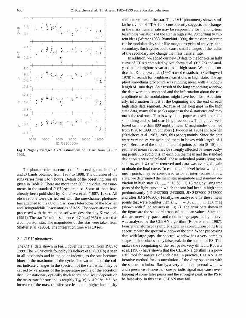
Fig. 1. Nightly averagedUBV estimations of TT Ari from 1985 to1999.

The photometric data consist of 45 observing runs in theUandB bands obtained from 1987 to 1998. The duration of theruns varies from 1 to 7 hours. Details of the observing runs aregiven in Table 2. There are more than 600 individual measure-ments in the standardUBV system also. Some of them havealready been published by Kraicheva et al. (1987, 1989). Allobservations were carried out with the one-channel photome-ters attached to the 60-cm Carl Zeiss telescopes of the Rozhenand Belogradchik Observatories of BAS. The observations wereprocessed with the reduction software described by Kirov et al.(1991). The star “c” of the sequence of Gotz (1985) was used asa comparison star. The magnitudes of this star were taken fromShafter et al. (1985). The integration time was 10 sec.

2.1. UBV photometry

TheUBV data shown in Fig. 1 cover the interval from 1985 to1999. The∼ 6 yr cycle found by Kraicheva et al. (1997b) is seenin all passbands and in the color indexes, as the star becomesbluer in the maximum of the cycle. The variations of the col-ors indicate changes in the spectrum of the star, which may becaused by variations of the temperature profile of the accretiondisc. For stationary optically thick accretion discs it depends onthe mass transfer rate and is roughlyTeff(r) ∼ M1/4r−3/4. Anincrease of the mass transfer rate leads to a higher luminosity

and bluer colors of the star. TheUBV photometry shows simi-lar behaviour of TT Ari and consequently suggests that changesin the mass transfer rate may be responsible for the long-termbrightness variations of the star in high state. According to cur-rent ideas (Warner 1988; Bianchini 1990), the mass transfer ratecan be modulated by solar-like magnetic cycles of activity in thesecondary. Such cycles could cause small changes of the radiusof the secondary and change the mass transfer rate.

In addition, we added our newB data to the long-term lightcurve of TT Ari compiled by Kraicheva et al. (1997b) and anal-ysed it for brightness variations in high state. We should no-tice that Kraicheva et al. (1997b) usedθ-statistics (Stellingwerf1978) to search for brightness variations in high state. The ap-plied smoothing procedure was running mean with a windowlength of 1000 days. As a result of the long smoothing window,the data were too smoothed and the information about the trueamplitude of the modulations might have been lost. Addition-ally, information is lost at the beginning and the end of eachhigh state data segment. Because of the long gaps in the highstate data, many false peaks appear in theθ-statistics and maymask the real ones. That is why in this paper we used other datasmoothing and period searching procedures. The light curve isbased on more than 800 nightly meanB magnitudes obtainedfrom 1928 to 1999 in Sonneberg (Hudec et al. 1984) and Rozhen(Kraicheva et al. 1987, 1989, this paper) mainly. Since the datawere very noisy, we averaged them in boxes with length of 1year. Because of the small number of points per bin (5–15), theestimated mean values may be strongly affected by some outly-ing points. To avoid this, in each bin the mean and the standarddeviationσ were calculated. Those individual points lying out-sidemean ± 3σ were removed and data was averaged againto obtain the final curve. To estimate the level below which themean points may be considered to be at intermediate or lowstate, we determined the mean star magnitude and standard de-viation in high stateBmean ' 10.60 ± 0.13 mag by using treeparts of the light curve in which the star had been in high statepredominantly (JD 2427000–2430000, JD 2437000–2443000and after JD 2446500). Finally, we analysed only those meanpoints that were brighter thanBmean + 3 σBmean

' 11.0 mag(shown with filled squares in Fig. 2). The error bars shown inthe figure are the standard errors of the mean values. Since thedata are unevenly spaced and contain large gaps, the light curvewas analysed by the CLEAN algorithm (Roberts et al. 1987).Fourier transform of a sampled signal is a convolution of the truespectrum with the spectral window of the data. When processingdata with large gaps, the spectral window has a very complexshape and introduces many false peaks in the computed PS. Thismakes the recognizing of the real peaks very difficult. Robertset al. (1987) have shown that the CLEAN algorithm is a pow-erful tool for analysis of such data. In practice, CLEAN is aniterative method for deconvolution of the dirty spectrum withthe spectral window. Rarely, a very complex spectral windowand a presence of more than one periodic signal may cause over-lapping of some false peaks and the strongest peak in the PS tobe false also. In this case CLEAN may fail.

Z. Kraicheva et al.: TT Arietis: 1985–1999 accretion disc behaviour 609

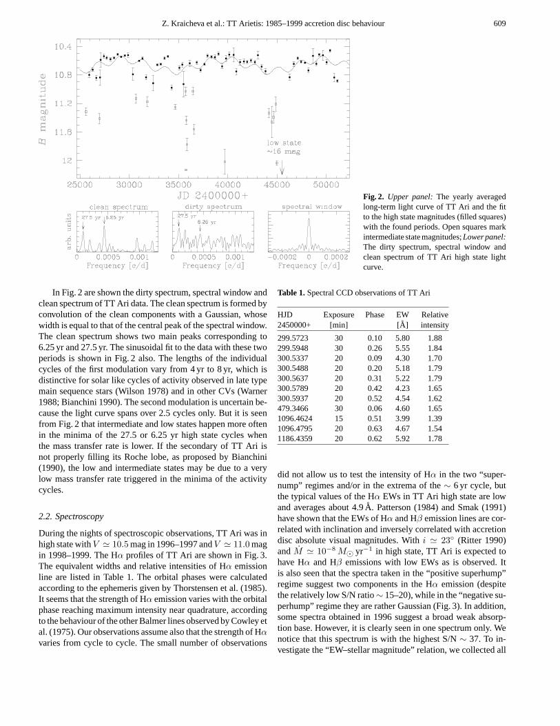
Fig. 2. Upper panel:The yearly averagedlong-term light curve of TT Ari and the fitto the high state magnitudes (filled squares)with the found periods. Open squares markintermediate state magnitudes;Lower panel:The dirty spectrum, spectral window andclean spectrum of TT Ari high state lightcurve.

In Fig. 2 are shown the dirty spectrum, spectral window andclean spectrum of TT Ari data. The clean spectrum is formed byconvolution of the clean components with a Gaussian, whosewidth is equal to that of the central peak of the spectral window.The clean spectrum shows two main peaks corresponding to6.25 yr and 27.5 yr. The sinusoidal fit to the data with these twoperiods is shown in Fig. 2 also. The lengths of the individualcycles of the first modulation vary from 4 yr to 8 yr, which isdistinctive for solar like cycles of activity observed in late typemain sequence stars (Wilson 1978) and in other CVs (Warner1988; Bianchini 1990). The second modulation is uncertain be-cause the light curve spans over 2.5 cycles only. But it is seenfrom Fig. 2 that intermediate and low states happen more oftenin the minima of the 27.5 or 6.25 yr high state cycles whenthe mass transfer rate is lower. If the secondary of TT Ari isnot properly filling its Roche lobe, as proposed by Bianchini(1990), the low and intermediate states may be due to a verylow mass transfer rate triggered in the minima of the activitycycles.

2.2. Spectroscopy

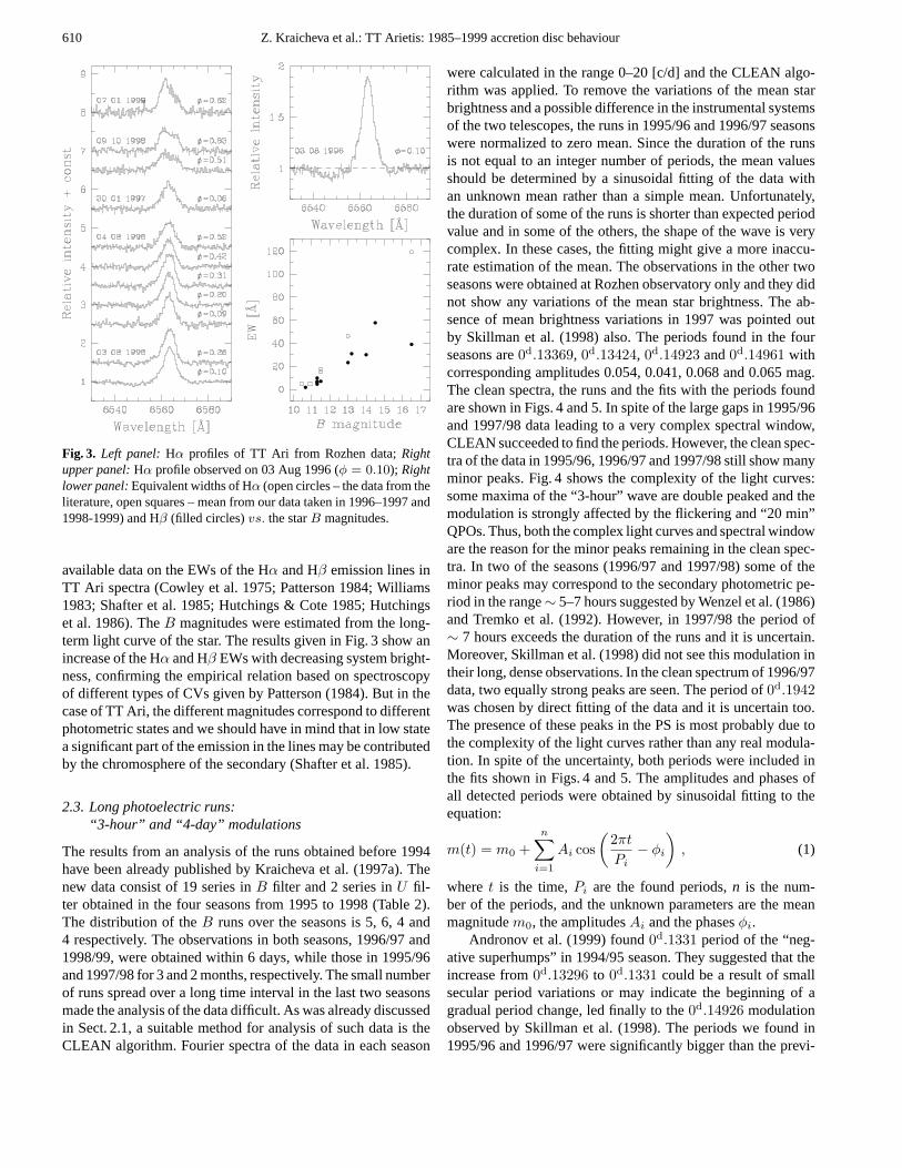
During the nights of spectroscopic observations, TT Ari was inhigh state withV ' 10.5 mag in 1996–1997 andV ' 11.0 magin 1998–1999. The Hα profiles of TT Ari are shown in Fig. 3.The equivalent widths and relative intensities of Hα emissionline are listed in Table 1. The orbital phases were calculatedaccording to the ephemeris given by Thorstensen et al. (1985).It seems that the strength of Hα emission varies with the orbitalphase reaching maximum intensity near quadrature, accordingto the behaviour of the other Balmer lines observed by Cowley etal. (1975). Our observations assume also that the strength of Hαvaries from cycle to cycle. The small number of observations

Table 1.Spectral CCD observations of TT Ari

HJD Exposure Phase EW Relative2450000+ [min] [A] intensity

299.5723 30 0.10 5.80 1.88299.5948 30 0.26 5.55 1.84300.5337 20 0.09 4.30 1.70300.5488 20 0.20 5.18 1.79300.5637 20 0.31 5.22 1.79300.5789 20 0.42 4.23 1.65300.5937 20 0.52 4.54 1.62479.3466 30 0.06 4.60 1.651096.4624 15 0.51 3.99 1.391096.4795 20 0.63 4.67 1.541186.4359 20 0.62 5.92 1.78

did not allow us to test the intensity of Hα in the two “super-nump” regimes and/or in the extrema of the∼ 6 yr cycle, butthe typical values of the Hα EWs in TT Ari high state are lowand averages about 4.9A. Patterson (1984) and Smak (1991)have shown that the EWs of Hα and Hβ emission lines are cor-related with inclination and inversely correlated with accretiondisc absolute visual magnitudes. Withi ' 23◦ (Ritter 1990)andM ' 10−8 M� yr−1 in high state, TT Ari is expected tohave Hα and Hβ emissions with low EWs as is observed. Itis also seen that the spectra taken in the “positive superhump”regime suggest two components in the Hα emission (despitethe relatively low S/N ratio∼ 15–20), while in the “negative su-perhump” regime they are rather Gaussian (Fig. 3). In addition,some spectra obtained in 1996 suggest a broad weak absorp-tion base. However, it is clearly seen in one spectrum only. Wenotice that this spectrum is with the highest S/N∼ 37. To in-vestigate the “EW–stellar magnitude” relation, we collected all


Fig. 3. Left panel:Hα profiles of TT Ari from Rozhen data;Rightupper panel:Hα profile observed on 03 Aug 1996 (φ = 0.10); Rightlower panel:Equivalent widths of Hα (open circles – the data from theliterature, open squares – mean from our data taken in 1996–1997 and1998-1999) and Hβ (filled circles)vs. the starB magnitudes.

available data on the EWs of the Hα and Hβ emission lines inTT Ari spectra (Cowley et al. 1975; Patterson 1984; Williams1983; Shafter et al. 1985; Hutchings & Cote 1985; Hutchingset al. 1986). TheB magnitudes were estimated from the long-term light curve of the star. The results given in Fig. 3 show anincrease of the Hα and Hβ EWs with decreasing system bright-ness, confirming the empirical relation based on spectroscopyof different types of CVs given by Patterson (1984). But in thecase of TT Ari, the different magnitudes correspond to differentphotometric states and we should have in mind that in low statea significant part of the emission in the lines may be contributedby the chromosphere of the secondary (Shafter et al. 1985).

2.3. Long photoelectric runs:“3-hour” and “4-day” modulations

The results from an analysis of the runs obtained before 1994have been already published by Kraicheva et al. (1997a). Thenew data consist of 19 series inB filter and 2 series inU fil-ter obtained in the four seasons from 1995 to 1998 (Table 2).The distribution of theB runs over the seasons is 5, 6, 4 and4 respectively. The observations in both seasons, 1996/97 and1998/99, were obtained within 6 days, while those in 1995/96and 1997/98 for 3 and 2 months, respectively. The small numberof runs spread over a long time interval in the last two seasonsmade the analysis of the data difficult. As was already discussedin Sect. 2.1, a suitable method for analysis of such data is theCLEAN algorithm. Fourier spectra of the data in each season

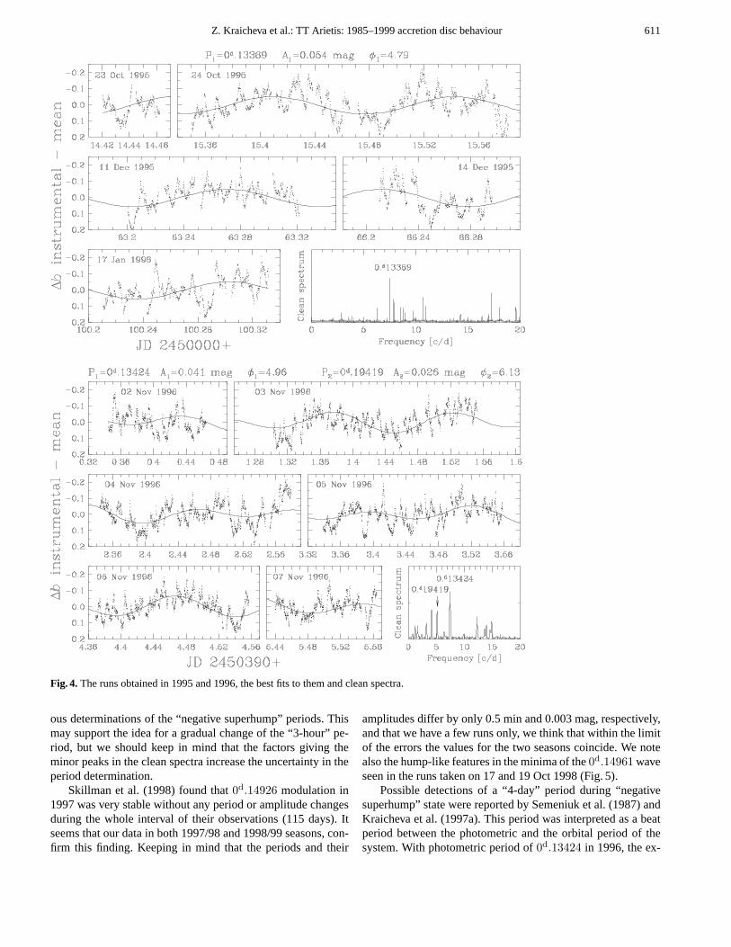
were calculated in the range 0–20 [c/d] and the CLEAN algo-rithm was applied. To remove the variations of the mean starbrightness and a possible difference in the instrumental systemsof the two telescopes, the runs in 1995/96 and 1996/97 seasonswere normalized to zero mean. Since the duration of the runsis not equal to an integer number of periods, the mean valuesshould be determined by a sinusoidal fitting of the data withan unknown mean rather than a simple mean. Unfortunately,the duration of some of the runs is shorter than expected periodvalue and in some of the others, the shape of the wave is verycomplex. In these cases, the fitting might give a more inaccu-rate estimation of the mean. The observations in the other twoseasons were obtained at Rozhen observatory only and they didnot show any variations of the mean star brightness. The ab-sence of mean brightness variations in 1997 was pointed outby Skillman et al. (1998) also. The periods found in the fourseasons are0d.13369, 0d.13424, 0d.14923 and0d.14961 withcorresponding amplitudes 0.054, 0.041, 0.068 and 0.065 mag.The clean spectra, the runs and the fits with the periods foundare shown in Figs. 4 and 5. In spite of the large gaps in 1995/96and 1997/98 data leading to a very complex spectral window,CLEAN succeeded to find the periods. However, the clean spec-tra of the data in 1995/96, 1996/97 and 1997/98 still show manyminor peaks. Fig. 4 shows the complexity of the light curves:some maxima of the “3-hour” wave are double peaked and themodulation is strongly affected by the flickering and “20 min”QPOs. Thus, both the complex light curves and spectral windoware the reason for the minor peaks remaining in the clean spec-tra. In two of the seasons (1996/97 and 1997/98) some of theminor peaks may correspond to the secondary photometric pe-riod in the range∼ 5–7 hours suggested by Wenzel et al. (1986)and Tremko et al. (1992). However, in 1997/98 the period of∼ 7 hours exceeds the duration of the runs and it is uncertain.Moreover, Skillman et al. (1998) did not see this modulation intheir long, dense observations. In the clean spectrum of 1996/97data, two equally strong peaks are seen. The period of0d.1942was chosen by direct fitting of the data and it is uncertain too.The presence of these peaks in the PS is most probably due tothe complexity of the light curves rather than any real modula-tion. In spite of the uncertainty, both periods were included inthe fits shown in Figs. 4 and 5. The amplitudes and phases ofall detected periods were obtained by sinusoidal fitting to theequation:

m(t) = m0 +n∑

i=1

Ai cos(

2πt

Pi− φi

), (1)

wheret is the time,Pi are the found periods,n is the num-ber of the periods, and the unknown parameters are the meanmagnitudem0, the amplitudesAi and the phasesφi.

Andronov et al. (1999) found0d.1331 period of the “neg-ative superhumps” in 1994/95 season. They suggested that theincrease from0d.13296 to 0d.1331 could be a result of smallsecular period variations or may indicate the beginning of agradual period change, led finally to the0d.14926 modulationobserved by Skillman et al. (1998). The periods we found in1995/96 and 1996/97 were significantly bigger than the previ-


Fig. 4. The runs obtained in 1995 and 1996, the best fits to them and clean spectra.

ous determinations of the “negative superhump” periods. Thismay support the idea for a gradual change of the “3-hour” pe-riod, but we should keep in mind that the factors giving theminor peaks in the clean spectra increase the uncertainty in theperiod determination.

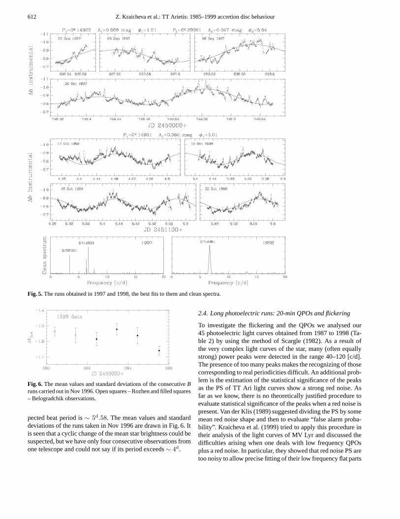
Skillman et al. (1998) found that0d.14926 modulation in1997 was very stable without any period or amplitude changesduring the whole interval of their observations (115 days). Itseems that our data in both 1997/98 and 1998/99 seasons, con-firm this finding. Keeping in mind that the periods and their

amplitudes differ by only 0.5 min and 0.003 mag, respectively,and that we have a few runs only, we think that within the limitof the errors the values for the two seasons coincide. We notealso the hump-like features in the minima of the0d.14961 waveseen in the runs taken on 17 and 19 Oct 1998 (Fig. 5).

Possible detections of a “4-day” period during “negativesuperhump” state were reported by Semeniuk et al. (1987) andKraicheva et al. (1997a). This period was interpreted as a beatperiod between the photometric and the orbital period of thesystem. With photometric period of0d.13424 in 1996, the ex-


Fig. 5. The runs obtained in 1997 and 1998, the best fits to them and clean spectra.

Fig. 6. The mean values and standard deviations of the consecutiveBruns carried out in Nov 1996. Open squares – Rozhen and filled squares– Belogradchik observations.

pected beat period is∼ 5d.58. The mean values and standarddeviations of the runs taken in Nov 1996 are drawn in Fig. 6. Itis seen that a cyclic change of the mean star brightness could besuspected, but we have only four consecutive observations fromone telescope and could not say if its period exceeds∼ 4d.

2.4. Long photoelectric runs: 20-min QPOs and flickering

To investigate the flickering and the QPOs we analysed our45 photoelectric light curves obtained from 1987 to 1998 (Ta-ble 2) by using the method of Scargle (1982). As a result ofthe very complex light curves of the star, many (often equallystrong) power peaks were detected in the range 40–120 [c/d].The presence of too many peaks makes the recognizing of thosecorresponding to real periodicities difficult. An additional prob-lem is the estimation of the statistical significance of the peaksas the PS of TT Ari light curves show a strong red noise. Asfar as we know, there is no theoretically justified procedure toevaluate statistical significance of the peaks when a red noise ispresent. Van der Klis (1989) suggested dividing the PS by somemean red noise shape and then to evaluate “false alarm proba-bility”. Kraicheva et al. (1999) tried to apply this procedure intheir analysis of the light curves of MV Lyr and discussed thedifficulties arising when one deals with low frequency QPOsplus a red noise. In particular, they showed that red noise PS aretoo noisy to allow precise fitting of their low frequency flat parts


Fig. 7. The light curves of TT Ari obtainedon Oct 13, 1993 and Oct 25, 1989 and theirpower spectra.

and it is hard to determine the smooth red noise shape by thisway. However, if we search for QPOs in the low frequency flatpart of the PS, “false alarm probability” may be used withoutany normalisation. In the case of TT Ari, the power in the QPOsis near the turnover of the PS (Fig. 8) and a normalisation isneeded, thus, we did not try to estimate statistical significancesof the peaks. In this case a more suitable procedure would beto perform sine fits to the data with all detected periods. Sincethe light curves are sawtooth rather than sinusoidal, an exact fitis not possible, but a careful inspection of the fits could give anidea about the real periodicities. In addition, multi-frequencyfits with combinations between all detected periods could beuseful.

The main result of the frequency analysis and data fittingis that the “20-min” QPOs in TT Ari are highly unstable. Inspite of the many power peaks detected in the range 40–120[c/d], there are no single oscillations that can describe a givenrun completely. Instead, in most of the runs, distinct parts couldbe fitted well by sinusoids with quite different periods rangingfrom 4 min to 26 min. The fits showed that these oscillationsremained coherent for about 3–8 cycles and in most runs thedistinct parts did not overlap. As examples, the series obtainedon 25 Oct 1989 and 13 Oct 1993 are given in Fig. 7.

Light curves showing transient oscillations with varying pe-riods, phases and amplitudes can be modelled by autoregressiveprocesses (Robinson & Nather 1979). An autoregressive processof orderp (AR(p)) is defined by the equation:

xj =p∑

i=1

aixj−i + εj , (2)

whereai are the filter coefficients andε denotes an uncorrelatedwhite noise process with zero mean and varianceσ2. If thecoefficientsai are chosen properly, Eq. 2 describes the sum ofdumped oscillators. Of particular interest for astronomy are twospecial cases: AR(1) and AR(2). The former may be recognisedas a usual “shot noise” process which assumes the light curveas a sum of randomly occurring exponentially decaying shots.If the two parameters of an AR(2) process fulfil the conditiona21 + 4 a2 < 0, it corresponds to a dumped oscillator with char-

acteristic period and dumping time determined by the particularvalues of the coefficients. Since the process is driven by a ran-dom noise, it is completely unpredictable and the resulting lightcurves are the sum of dumped oscillations with randomly vary-ing period and phase. The PS of such processes show a singlebroad peak (Robinson & Nather 1979). If the coefficients do notfulfil the above condition, Eq. 2 describes a “shot noise” processbut the shots are no longer simple exponents. Having the ARcoefficients estimated, the PS of the process can be calculated.

The calculation of AR model coefficients is a linear problemand many efficient numerical algorithms have been developed.We used that published by Andersen (1974). Since the runscontained gaps, we adapted the algorithm to adjust AR modelcoefficients using only available data. The most difficult prob-lem is the choice of the AR model order. For that purpose theFinal Prediction Error (FPE) criterion (Akaike 1970) was used,namely, the correct model order is that minimising the quantity:

FPE(m) =N + k (m + 1)N − k (m + 1)

S2m , (3)

whereN is the number of data points,m is the AR model order,k is the number of data segments andSm is the output error


of the filter. Eq. 3 differs from the original FPE criterion by thefactork, which takes into account the fact that AR coefficientsare computed fromk data segments. The procedure was testedwith simulated AR series and it was found that it determines boththe AR coefficients and the model order correctly. AR modelshave the property that, if the model order is correctly chosen, thecalculated PS are optimally smooth. Before the calculation ofthe AR coefficients, the “3-hour” waves were removed from thedata. This was done by subtraction of a cubic spline through themean points in non-overlapping bins of length∼ 20 min. Thespline interpolation was calculated by using a subroutine basedon the tension spline algorithms given by Cline (1974). Thetension splines are less likely to introduce spurious inflectionpoints. The algorithm allows the tension in the interpolatingcurve to be a free parameter. If the tension is close to zero(' 0.01), the interpolating curve is almost natural cubic splineand if it is large (≥ 10), the curve is almost polygonal line. Weused tension of 1.

The calculations showed that most of TT Ari light curvescould be modelled as AR(1) and AR(2) processes and only a fewas AR(3). There are at least two factors that can influence ARcoefficient estimation and FPE: observational noise and trendremoval. In Eq. 2,ε is a random variable that only drives theAR process and any other noise processes are not taken intoaccount. The real light curves, however, are always covered byobservational noise. The numerical algorithm used cannot sep-arate these two noise processes and the observational noise istreated as an addition toε. Besides, any trend removal intro-duces residual noise. This noise was discussed by Kraichevaet al. (1999) and they concluded that if a cubic spline throughmean points in long enough bins is subtracted, the residual noiseshould be small compared with characteristic amplitude of theflickering and it should weakly affect the results. Thus, the factthat we found different AR model orders does not mean that thelight curves have different properties. This is most probably dueto the influence of the noise. The most important result is thatall PS of the estimated AR models follow roughly the shape:

P (f) ∝ 11 + (2πτf)γ

. (4)

without any peaks seen. Heref is the frequency andγ is theslope of the PS in the high frequencies. Ifγ=2, Eq. 4 exactlydescribes the PS of the usual “shot noise” process andτ is thee-folding constant of the exponential shots.

In general, any AR(p) process can be converted into an in-finitely long moving average (MA) process defined by the equa-tion:

xj =∞∑

i=0

biεj−i , (5)

whereε is again an uncorrelated white noise process and the fil-terbi is the inverse ofai (Scargle 1981). The MA representationhas a more clear meaning than the AR one: Eq. 5 describes thereaction of the system to a random impulse sequence. Thus inthe case of stochastic processes, MA representation is more rea-sonable. As can be seen from Eq. 5, the usual “shot noise” pro-

cesses are a special case of MA whenεi is a Poisson sequence,bi = e−i∆/τ and where∆ is the time step. In the common case,the MA filter coefficients may be arbitrary (the only restrictionis the filter to be stable, i.e.

∑∞i=0 b2

i < ∞). The fact that the PSof the calculated AR models do not show peaks suggests thatfast variability of TT Ari can be modelled as a general “shotnoise” process. The strong low frequency variability in such aprocess is a result of the shots overlapping (Terebizh 1989). Ifthe overlapping parameter, i.e. the number of the shots per oneshot duration, is greater than 3–4, the “shot noise” process caneasily produce transient QPOs. Then, in some parts of finitelength series generated by such a “shot noise” process, tran-sient QPOs may be detected. Therefore it is possible the QPOsobserved in TT Ari light curves to be generated by the sameinstability mechanism as the flickering, i.e. the QPOs and theflickering could be the same thing. One may try to find the exactshape of the individual shots by an inversion of the estimatedAR parameters. As Scargle (1981) pointed out, the procedureof Andersen (1974) presumes that the AR filter is minimum de-lay. In astronomy this is rarely the case and the shape obtainedby the inversion may not be the real one. That is why we havenot tried to invert the AR coefficients and only emphasise theability of the “shot noise” processes to generate transient QPOsas those observed in TT Ari. However, the low frequency flatpart and the values of the power slope (Table 2) suggest that theshots are not far from a single exponent.

The flickering is often modelled in term of “shot noise” pro-cess and many authors (Williams & Hiltner 1984; Elsworth &James 1982; Panek 1980; Bruch 1992) suppose that it is respon-sible for the red noise observed in CVs. The flickering may becharacterised by some empirical quantities such as the powerlaw indexγ, the typical time scaleτ , amplitude and the emit-ted energy. They have been determined and published for manystars, and the theoretical or numerical models have to be con-sistent with them. The determination of all these quantities andthe difficulties related to it have been discussed by Kraicheva etal. (1999) and here we only mention some of the key points.

All estimated quantities are given in Table 2. As estimationsof the flickering activity, the total amplitude (i.e. the differencebetween the brightest and the faintest points in the light curve)and the standard deviation around the mean of the light curvesare listed in the table. If these quantities are taken as activityindications, it seems that there is no difference of the flickeringactivity in B andU bands.

The contribution of the flickering light source to the totallight of the star can be estimated following the conception ofBruch (1992). The brightness of the star can be considered asa sum of the flickering light sourceFf and all other sourcesFcsupposed to be constant on the flickering time scale. An upperlimit of the constant light source magnitude can be defined asmc = m+∆m/2, wherem is the mean star magnitude and∆mis the total amplitude of the flickering. Then, if the amplitudeof the flickering is assumed to be independent of the passband,the ratio of the flux of the flickering light source to that of theconstant one, over the whole optical range, is given by


Table 2.Flickering properties

No UT date Filter Start time Length γ τ Standard AmplitudeFf,mean

Fc

Ff,maxFc

[UT] [hours] [sec] deviation [mag]

1 1987 Aug 25 U 23h30m 2.10 2.14 153.8 0.052 0.223 0.108 0.2352 1987 Aug 31 U 23h10m 1.92 1.94 150.2 0.066 0.333 0.166 0.4343 1987 Sep 01 U 21h55m 2.80 2.14 109.3 0.071 0.475 0.244 0.5384 1987 Dec 07 U 20h15m 3.36 1.94 105.7 0.054 0.261 0.128 0.2495 1988 Jan 18 U 17h40m 2.30 2.12 120.5 0.060 0.360 0.180 0.4786 1988 Aug 20 U 22h50m 2.45 1.80 141.5 0.054 0.397 0.200 0.3957 1988 Sep 12 B 22h55m 3.36 2.20 178.6 0.067 0.600 0.318 0.5178 1988 Sep 13 B 22h40m 3.12 2.01 115.3 0.042 0.252 0.123 0.2759 1989 Jan 31 B 18h07m 1.42 1.82 89.0 0.032 0.186 0.090 0.17510 1989 Aug 01 U 23h47m 1.20 2.00 102.5 0.046 0.274 0.135 0.31411 1989 Aug 28 U 22h10m 3.00 2.27 152.0 0.057 0.288 0.142 0.33912 1989 Oct 24 U 20h50m 4.08 2.32 134.8 0.063 0.371 0.186 0.42113 1989 Oct 25 U 19h50m 4.92 2.03 115.1 0.043 0.323 0.161 0.40814 1989 Oct 28 B 20h30m 1.40 2.06 75.0 0.037 0.267 0.131 0.25015 1989 Oct 29 B 21h00m 3.90 2.12 196.5 0.041 0.241 0.117 0.25816 1990 Jan 24 U 18h57m 1.32 1.89 139.2 0.050 0.227 0.110 0.25517 1990 Oct 11 U 23h04m 2.04 2.28 141.4 0.075 0.446 0.228 0.63818 1990 Oct 13 U 00h30m 1.32 2.33 105.7 0.050 0.300 0.148 0.41319 1990 Oct 13 U 23h55m 2.08 1.95 119.7 0.108 0.669 0.361 0.66220 1990 Oct 15 U 22h40m 3.67 2.12 111.4 0.057 0.365 0.183 0.45821 1991 Jan 25 U 18h05m 2.30 2.15 114.0 0.058 0.336 0.168 0.40822 1991 Jan 26 U 17h45m 2.50 1.96 152.7 0.062 0.315 0.156 0.35023 1992 Dec 18 U 18h55m 3.62 2.23 126.5 0.062 0.363 0.182 0.41024 1992 Dec 19 B 18h00m 2.06 2.60 114.4 0.053 0.293 0.145 0.36625 1993 Oct 13 U 22h52m 2.68 2.36 127.9 0.057 0.310 0.154 0.36626 1994 Dec 04 B 19h37m 2.25 1.91 183.0 0.062 0.338 0.168 0.41927 1995 Oct 24 B 20h17m 5.52 2.08 142.2 0.053 0.308 0.152 0.35028 1995 Dec 11 B 16h47m 2.90 2.14 130.9 0.053 0.292 0.144 0.30129 1995 Dec 14 B 17h00m 2.06 2.00 170.6 0.062 0.298 0.147 0.32430 1996 Jan 17 B 17h08m 2.88 2.07 180.7 0.066 0.386 0.194 0.45531 1996 Sep 11 U 23h42m 2.25 1.93 195.1 0.083 0.430 0.219 0.43732 1996 Nov 02 B 20h10m 2.76 2.00 155.8 0.052 0.273 0.134 0.32633 1996 Nov 03 B 19h10m 6.00 2.07 132.0 0.048 0.310 0.153 0.33834 1996 Nov 04 B 20h10m 5.60 2.02 221.8 0.051 0.315 0.156 0.35635 1996 Nov 04 U 19h22m 5.16 2.07 206.0 0.066 0.354 0.177 0.40436 1996 Nov 05 B 20h00m 5.28 2.07 211.8 0.055 0.370 0.186 0.44837 1996 Nov 06 B 20h45m 4.51 2.07 149.2 0.048 0.281 0.138 0.34038 1996 Nov 07 B 20h30m 2.94 2.16 200.3 0.046 0.282 0.138 0.30039 1997 Sep 06 B 00h17m 2.08 1.74 168.7 0.030 0.160 0.076 0.17940 1997 Sep 07 B 00h00m 2.42 1.77 146.3 0.035 0.180 0.086 0.18241 1997 Oct 26 B 20h32m 7.13 1.84 166.0 0.031 0.220 0.107 0.25042 1998 Oct 17 B 20h23m 6.08 1.74 148.2 0.023 0.184 0.088 0.22643 1998 Oct 18 B 21h38m 4.09 1.71 166.3 0.029 0.172 0.082 0.19944 1998 Oct 19 B 18h52m 7.68 1.74 126.2 0.018 0.126 0.059 0.13845 1998 Oct 22 B 23h00m 3.52 1.68 161.7 0.021 0.167 0.080 0.192

Ff

Fc= 10−0.4∆m′ − 1 (6)

where∆m′ = m0 −mc andm0 is the magnitude of some pointof the light curve. In Table 2 the ratios of the fluxes calculatedfor m0 equal to the mean and the maximal star brightness aregiven. Asmc is an upper limit for the constant light source,the calculated ratios have to be considered as a lower limit. The

estimated values suggest that a significant part of the visual lightof TT Ari is emitted by the flickering light source.

The power law indexγ was determined by least-squareslinear fitting of the high frequency linear parts of the PS in log-log scale. The interval in which the fits were performed variedfrom 100–120 [c/d] to 1700–2000 [c/d] depending on the qualityof the light curves. Small changes in this interval caused changes


Fig. 8. The mean seasonal power spectra of TT Ari fitted by Eq. 4.

of the values ofγ reaching 0.2–0.3 and this is the real error inthe determination ofγ. The values ofγ vary, but the average isabout 2. The fact that all PS have a shape similar to that definedby Eq. 4 andγ’s are≈ 2, suggests that the underlying physicalprocess could be mathematically described by a “shot noise”process with shot differing from exponents a little.

Since strong shot overlapping is expected, the duration ofthe shotsτ cannot be directly measured. One way to estimate itis by autocorrelation function (ACF).τ may be defined as thetime shift at which the ACF,r(τ), first reaches valuer0 = 1/e.The ACF of an infinitely long “shot noise” process has a shaper(t) ∝ exp(−t/τ), wheret is the shift time andτ is the e-folding constant of the exponential shots. Because of the finitelength of the observational data, the ACF is strongly biasedby the shots overlapping and it does not follow this theoreticalshape. Instead of this, it crosses the zero level at some lag andafter that oscillates around it. Additionally, the ACF is biasedby trend removal and observational noise. A precise analyticaltheory of bias of ACF owed to all these factors can be found inAndronov (1994). In spite of the fact that the common shape ofthe ACF is strongly biased, using simulated “shot noise” series,Kraicheva et al. (1999) showed that a mean of several valuesmight be a correct estimation ofτ . For shots with arbitrary shape,the τ ’s calculated by ACF may be considered as an effectiveduration or in case of varying duration, as a mean. In general,τcould be determined by direct fitting of the PS to the Eq. 4. Buthere, we have the same problem as that in the determination ofthe mean red noise shape of the PS, discussed in the beginning ofthis section. Thus, we give preference to the theτ ’s determinedby the ACF.

In Fig. 8 are shown the mean PS for the six seasons bestcovered by observations in log-log scale and the fits obtained

by Eq. 4. The fits were performed withγ andτ fixed to valuespreviously determined and the only unknown parameter was aconstant multiplying Eq. 4.γ’s were determined from the meanspectra as was discussed above andτ ’s are the mean of theindividual determinations. To avoid the influence of the powerexcess due to the “3-hour” modulations, the PS were fitted forfrequencieslog(f) ≥ 1.25 only. In spite of some deviationsfrom the fits near the turnover, it is seen that the shape of the PSis described by Eq. 4.

3. Discussion

The analysis of our data shows that the “positive superhump” inTT Ari light curves has remained “active” for more than a year.A comparison between Figs. 4 and 5 shows that the “positivesuperhump” is more stable than the “negative” one; while thedata in 1997–1998 are almost perfectly fitted, the fits of 1995–1996 data deviate in some parts of the curves. Moreover, theamplitude of the∼ 0d.14926 wave is larger than that of the∼ 0d.1330 signal. On the basis of the fact that with a “positivesuperhump” period of∼ 0d.14926 TT Ari follows the “orbitalperiod–fractional period excess” relation for the CVs showing“positive superhumps”, Skillman et al. (1998) supposed that thenew wave in TT Ari could be a “positive superhump” of the sametype. There are, however, some uncertainties related to this in-terpretation. The “positive superhumps” observed in SU UMatype CVs during superoutburst are thought to arise from a slowlyprecessing under the gravity of the orbiting secondary eccen-tric accretion disc. The theoretical and numerical analyses haveshown that eccentric accretion discs are formed under the ac-tion of 3:1 resonance, where the accretion disc matter orbits ata period 3 times shorter than the orbital one (Whitehurst 1988;Hirose & Osaki 1990; Lubow 1991). This resonance lies withinthe accretion disc only for systems with mass ratioq ≤ 0.3 andtherefore only these systems are expected to display “positivesuperhumps”. The mass ratio of TT Ari components is mostprobably' 0.5 (Ritter 1990) and the 3:1 resonance lies out-side the disc. The “positive superhump” phenomenon has beenobserved in other systems withq > 0.3 also (Patterson et al.1993; Skillman et al. 1995) and this suggests that another mech-anism of eccentric instability could operate. The origin of the“negative superhumps” in TT Ari light curves is unclear also.Lubow (1992) has shown that fluid discs are tilt unstable at the3:1 resonance. Patterson et al. (1993) supposed that “negativesuperhumps” in CVs arose from precession of a tilted disc, butthis model has the same problem – in TT Ari the 3:1 resonancemost likely lies outside the disc. Murray & Armigate (1998) haveinvestigated the tidal instabilities in CV accretion discs by 3Dnumerical simulations and found that the tilt instability couldnot grow fast enough to generate a significant tilt. Thus, thequestions concerning the origin of the “positive” and “negativesuperhumps” remain to be resolved by future investigations.

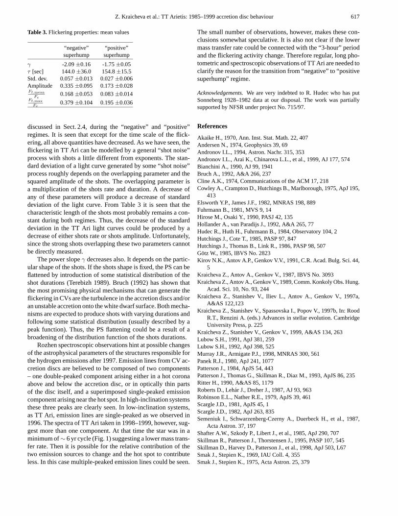
Our photometry before and after the “3-hour” period changeprovides us with an opportunity to search for changes in theobservational properties of the star. In Table 3 are listed themean values of the quantities characterising the flickering, as


Table 3.Flickering properties: mean values

“negative” “positive”superhump superhump

γ -2.09±0.16 -1.75±0.05τ [sec] 144.0±36.0 154.8±15.5Std. dev. 0.057±0.013 0.027±0.006Amplitude 0.335±0.095 0.173±0.028Ff,mean

Fc0.168±0.053 0.083±0.014

Ff,maxFc

0.379±0.104 0.195±0.036

discussed in Sect. 2.4, during the “negative” and “positive”regimes. It is seen that except for the time scale of the flick-ering, all above quantities have decreased. As we have seen, theflickering in TT Ari can be modelled by a general “shot noise”process with shots a little different from exponents. The stan-dard deviation of a light curve generated by some “shot noise”process roughly depends on the overlapping parameter and thesquared amplitude of the shots. The overlapping parameter isa multiplication of the shots rate and duration. A decrease ofany of these parameters will produce a decrease of standarddeviation of the light curve. From Table 3 it is seen that thecharacteristic length of the shots most probably remains a con-stant during both regimes. Thus, the decrease of the standarddeviation in the TT Ari light curves could be produced by adecrease of either shots rate or shots amplitude. Unfortunately,since the strong shots overlapping these two parameters cannotbe directly measured.

The power slopeγ decreases also. It depends on the partic-ular shape of the shots. If the shots shape is fixed, the PS can beflattened by introduction of some statistical distribution of theshot durations (Terebizh 1989). Bruch (1992) has shown thatthe most promising physical mechanisms that can generate theflickering in CVs are the turbulence in the accretion discs and/oran unstable accretion onto the white dwarf surface. Both mecha-nisms are expected to produce shots with varying durations andfollowing some statistical distribution (usually described by apeak function). Thus, the PS flattening could be a result of abroadening of the distribution function of the shots durations.

Rozhen spectroscopic observations hint at possible changesof the astrophysical parameters of the structures responsible forthe hydrogen emissions after 1997. Emission lines from CV ac-cretion discs are believed to be composed of two components– one double-peaked component arising either in a hot coronaabove and below the accretion disc, or in optically thin partsof the disc itself, and a superimposed single-peaked emissioncomponent arising near the hot spot. In high-inclination systemsthese three peaks are clearly seen. In low-inclination systems,as TT Ari, emission lines are single-peaked as we observed in1996. The spectra of TT Ari taken in 1998–1999, however, sug-gest more than one component. At that time the star was in aminimum of∼ 6 yr cycle (Fig. 1) suggesting a lower mass trans-fer rate. Then it is possible for the relative contribution of thetwo emission sources to change and the hot spot to contributeless. In this case multiple-peaked emission lines could be seen.

The small number of observations, however, makes these con-clusions somewhat speculative. It is also not clear if the lowermass transfer rate could be connected with the “3-hour” periodand the flickering activity change. Therefore regular, long pho-tometric and spectroscopic observations of TT Ari are needed toclarify the reason for the transition from “negative” to “positivesuperhump” regime.

Acknowledgements.We are very indebted to R. Hudec who has putSonneberg 1928–1982 data at our disposal. The work was partiallysupported by NFSR under project No. 715/97.

References

Akaike H., 1970, Ann. Inst. Stat. Math. 22, 407Andersen N., 1974, Geophysics 39, 69Andronov I.L., 1994, Astron. Nachr. 315, 353Andronov I.L., Arai K., Chinarova L.L., et al., 1999, AJ 177, 574Bianchini A., 1990, AJ 99, 1941Bruch A., 1992, A&A 266, 237Cline A.K., 1974, Communications of the ACM 17, 218Cowley A., Crampton D., Hutchings B., Marlborough, 1975, ApJ 195,

413Elsworth Y.P., James J.F., 1982, MNRAS 198, 889Fuhrmann B., 1981, MVS 9, 14Hirose M., Osaki Y., 1990, PASJ 42, 135Hollander A., van Paradijs J., 1992, A&A 265, 77Hudec R., Huth H., Fuhrmann B., 1984, Observatory 104, 2Hutchings J., Cote T., 1985, PASP 97, 847Hutchings J., Thomas B., Link R., 1986, PASP 98, 507Gotz W., 1985, IBVS No. 2823Kirov N.K., Antov A.P., Genkov V.V., 1991, C.R. Acad. Bulg. Sci. 44,

5Kraicheva Z., Antov A., Genkov V., 1987, IBVS No. 3093Kraicheva Z., Antov A., Genkov V., 1989, Comm. Konkoly Obs. Hung.

Acad. Sci. 10, No. 93, 244Kraicheva Z., Stanishev V., Iliev L., Antov A., Genkov V., 1997a,

A&AS 122,123Kraicheva Z., Stanishev V., Spassovska I., Popov V., 1997b, In: Rood

R.T., Renzini A. (eds.) Advances in stellar evolution. CambridgeUniversity Press, p. 225

Kraicheva Z., Stanishev V., Genkov V., 1999, A&AS 134, 263Lubow S.H., 1991, ApJ 381, 259Lubow S.H., 1992, ApJ 398, 525Murray J.R., Armigate P.J., 1998, MNRAS 300, 561Panek R.J., 1980, ApJ 241, 1077Patterson J., 1984, ApJS 54, 443Patterson J., Thomas G., Skillman R., Diaz M., 1993, ApJS 86, 235Ritter H., 1990, A&AS 85, 1179Roberts D., Lehar J., Dreher J., 1987, AJ 93, 963Robinson E.L., Nather R.E., 1979, ApJS 39, 461Scargle J.D., 1981, ApJS 45, 1Scargle J.D., 1982, ApJ 263, 835Semeniuk I., Schwarzenberg-Czerny A., Duerbeck H., et al., 1987,

Acta Astron. 37, 197Shafter A.W., Szkody P., Libert J., et al., 1985, ApJ 290, 707Skillman R., Patterson J., Thorstensen J., 1995, PASP 107, 545Skillman D., Harvey D., Patterson J., et al., 1998, ApJ 503, L67Smak J., Stepien K., 1969, IAU Coll. 4, 355Smak J., Stepien K., 1975, Acta Astron. 25, 379


Smak J., 1991, In: Bertout C., Collin-Souffrin S., Lasota J.P. (eds.)Structure and Emission Propertiesof Accretion disks. Proceedingsof IAU Colloq. 129, The 6th Institute d’Astrophysique de Paris(IAP) Meeting, Paris, France, 2–6 July 1990, Gif-sur-Yvette, Edi-tions Frontieres, Gif-sur-Yvette, 247

Stellingwerf R.F., 1978, ApJ 224, 953Stolz N., Schoembs R., 1984, ApJ 312, 121Terebizh, 1989, Astrophysica 31, 75Thorstensen J., Smak J., Hessman F., 1985, PASP 97, 437Tremko J., Andronov I.L., Luthardt R., et al., 1992, IBVS No. 3763Tremko J., Andronov I.L., Chinarova L.L., et al., 1996, A&A 312, 121Udalski A., 1988, Acta Astron. 38, 315

van der Klis M., 1989, NATO ASI Ser., Ser. C., Math. Phys. Sci. 262,27

Volpi A., Natali G., D‘Antona F., 1988, A&A 193, 87Warner B., 1988, Nat 336, 129Wenzel W., Hudec R., Schilt R., Tremko J., 1992, Contrib. Astron. Obs.

Skalnate Pleso 22, 69Wenzel W., Bojack W., Cristescu C., et al., 1986, Preprint Astron. Inst.

Ondrejov No.38Whitehurst R., 1988, MNRAS 232, 35Williams G., 1983, ApJS 53, 523Williams G.A., Hiltner W.A., 1984, MNRAS 211, 629Wilson O.C., 1978, ApJ 205, 612

Documents

Astron. Astrophys. 351, 607–618 (1999) ASTRONOMY AND TT ...aa.springer.de/papers/9351002/2300607.pdf · 608 Z. Kraicheva et al.: TT Arietis: 1985–1999 accretion disc behaviour