Assumptions in the Normal Linear Regression Model

A1: There is a linear relationship between X and Y. A2: The error terms (and thus the Y’s at each X) have constant variance. A3: The error terms are independent. A4: The error terms (and thus the Y’s at each X) are normally distributed. Note: In practice, we are looking for a fairly symmetric distribution with no major outliers. Other things to check (Questions to ask): Q5: Are there any major outliers in the data (X, or combination of (X,Y))? Q6: Are there other possible predictors that should be included in the model?

Useful Plots for Checking Assumptions and Answering These Questions

Reminders: Residual = ei = ii YY ˆ− = observed Yi – predicted Yi Predicted Yi = iY = b0 + b1Xi , also called “fitted Yi”

Definition: The semi-studentized residual for unit i is MSEee i

i =*

Plot Useful for

Dotplot, stemplot, histogram of X’s Q5 Outliers in X; range of X values Residuals ei versus Xi or predicted iY A1 Linear, A2 Constant var., Q5 outliers SS resids e* versus Xi or predicted iY As above, but a better check for outliers Dotplot, stemplot, histogram of ei A4 Normality assumption Residuals ei versus time (if measured) A3 Dependence across time Residuals ei versus other predictors Q6 Predictors missing from model “Normal probability plot” of residuals A4 Normality assumption

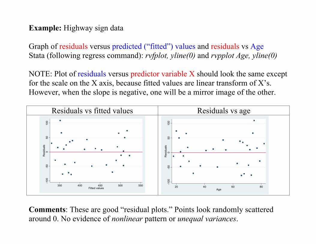
Example: Highway sign data Graph of residuals versus predicted (“fitted”) values and residuals vs Age Stata (following regress command): rvfplot, yline(0) and rvpplot Age, yline(0) NOTE: Plot of residuals versus predictor variable X should look the same except for the scale on the X axis, because fitted values are linear transform of X’s. However, when the slope is negative, one will be a mirror image of the other.

Residuals vs fitted values Residuals vs age

-100

-50

050

100

Res

idua

ls

350 400 450 500 550Fitted values

-100

-50

050

100

Res

idua

ls

20 40 60 80Age

Comments: These are good “residual plots.” Points look randomly scattered around 0. No evidence of nonlinear pattern or unequal variances.

Some other plots of the residuals: Normal probability plot of semi-studentized residuals (to check normality assumption, A4):

-2-1

01

2S

Sres

ids

-2 -1 0 1 2Inverse Normal

This is a pretty good plot. There is one point at each end that is slightly off, that might be investigated, but no major problems. Stata command (following regress): qnorm name where “name” is what you named the semi-studentized residuals.

Stemplot of semi-studentized residuals (to check normality assumption): stem SSresids Stem-and-leaf plot for SSresids SSresids rounded to nearest multiple of .01 plot in units of .01 -1** | 57,55 -1** | 45,42 -0** | 99,96,91,87,75,59,59 -0** | 25,23 0** | 05,13,17,20,23,30,35,48 0** | 60,70,78,86,99 1** | 30,32,48 1** | 2** | 19 This is further confirmation that the residuals are relatively symmetric with no major outliers. The 2.19 is for a driver with X = 75 years, Y = 460 feet.

What to do when assumptions aren’t met Assumption 1: Relationship is linear. How to detect a problem: Plot residuals versus fitted values. If you see a pattern, there is a problem with the assumption. What to do about the problem: Transform the X values, X' = f(X). Then do the regression using X' instead of X:

Y = β0 + β1 X' + ε

where we still assume the ε are N(0, σ2). NOTE: Only use this “solution” if non-linearity is the only problem, not if it also looks like there is non-constant variance or non-normal errors. For those, we will transform Y. REASON: The errors are in the vertical direction. Stretching or shrinking the X-axis doesn’t change those, so if they are normal with constant variance, they will stay that way. Let’s look at what kinds of transformations to use. (Also see page 130 in textbook.)

Residuals are inverted U, use X' = X or log10 X

X

Y

50403020100

160

140

120

100

80

60

40

20

Scatterplot of Y vs X

Fitted Value

Res

idua

l

1501251007550

15

10

5

0

-5

-10

-15

-20

-25

Residuals Versus the Fitted Values(response is Y)

Sqrt_X

Y

7654321

160

140

120

100

80

60

40

20

Scatterplot of Y vs Sqrt_X

Fitted Value

Res

idua

l

16014012010080604020

10

5

0

-5

-10

Residuals Versus the Fitted Values(response is Y)

Residuals are U-shaped and association between X and Y is positive: Use X' = X2

X

Yi

50403020100

3000

2500

2000

1500

1000

500

0

Scatterplot of Yi vs X

Fitted Value

Res

idua

l

25002000150010005000

500

250

0

-250

-500

Residuals Versus the Fitted Values(response is Yi)

X-squared

Yi

25002000150010005000

3000

2500

2000

1500

1000

500

0

Scatterplot of Yi vs X-squared

Fitted Value

Res

idua

l

300025002000150010005000

300

200

100

0

-100

-200

-300

Residuals Versus the Fitted Values(response is Yi)

Residuals are U-shaped and association between X and Y is negative: Use X' = 1/X or X' = exp(-X)

X

Y

0.50.40.30.20.10.0

9

8

7

6

5

4

3

2

1

0

Scatterplot of Y vs X

X

Res

idua

l

0.50.40.30.20.10.0

2

1

0

-1

-2

Residuals Versus X(response is Y)

1/X

Y

50403020100

9

8

7

6

5

4

3

2

Scatterplot of Y vs 1/X

1/X

Res

idua

l

50403020100

1.0

0.5

0.0

-0.5

-1.0

Residuals Versus 1/X(response is Y)

Assumption 2: Constant variance of the errors across X values. How to detect a problem: Plot residuals versus fitted values. If you see increasing or decreasing spread, there is a problem with the assumption. Example: Real estate data set C7 in Appendix C for n = 522 homes sold in a Midwestern city. Y = Sales price (thousands); X = Square feet (in hundreds). Original data:

020

040

060

080

010

00P

riceT

hsds

10 20 30 40 50SqFtHdrd

Residual plot:

-200

020

040

0R

esid

uals

10 20 30 40 50SqFtHdrd

Clearly, the variance is increasing as house size increases.

NOTE: Usually increasing variance and skewed distribution go together. Here is a histogram of the residuals, with a superimposed normal distribution. Notice the residuals extending to the right.

0.0

02.0

04.0

06.0

08D

ensi

ty

-200 0 200 400Residuals

What to do about the problem: Transform the Y values, or both the X and Y values. See page 132 for pictures. Example: Real estate sales, transform Y values to Y' = ln (Y) Scatter plot of ln(Price) vs Square feet

11.5

1212

.513

13.5

14Ln

Pric

e

1000 2000 3000 4000 5000SqFt

Residuals versus Square feet:

-1-.5

0.5

1R

esid

uals

1000 2000 3000 4000 5000SqFt

Looks like one more transformation might help – use square root of size. But we will leave it as this for now. See histogram of residual on next page.

0.5

11.

52

2.5

Den

sity

-1 -.5 0 .5 1Residuals

This looks better – more symmetric and no outliers.

Using models after transformations

Transforming X only: Use transformed X for future predictions: X' = f(X). Then do the regression using X' instead of X:

Y = β0 + β1 X' + ε

where we still assume the ε are N(0, σ2). For example, if X' = X then the predicted values are:

XbbY 10ˆ +=

Transforming Y (and possibly X): Everything must be done in transformed values. For confidence intervals and prediction intervals, get the intervals first and then transform the endpoints back to original units.

Example: Predicting house sales price using square feet. Regression equation is: Predicted Ln(Price) = 11.2824 + 0.051(Square feet in hundreds) For a house with 2000 square feet = 20 hundred square feet:

)20(051.02824.11'ˆ +=Y = 12.3024 So predicted price = exp(12.3024) = $220,224. 95% prediction interval for Ln(Price) is 11.8402, 12.7634. Transform back to dollars: Exp(11.8402) = $138,718 Exp( 12.7634) = $349,200 95% confidence interval for the mean Ln(Price) is 12.2803, 12.3233 Exp(12.2803) = $215,410 Exp(12.3233) = $224,875

Assumption 3: Independent errors 1. The main way to check this is to understand how the data were collected. For example, suppose we wanted to predict blood pressure from amount of fat consumed in the diet. If we were to sample entire families, and treat them as independent, that would be wrong. If one member of the family has high blood pressure, related members are likely to have it as well. Taking a random sample is one way to make sure the observations are independent. 2. If the values were collected over time (or space) it makes sense to plot the residuals versus order collected, and see if there is a trend or cycle. See page 109 for examples.

OUTLIERS

Some reasons for outliers: 1. A mistake was made. If it’s obvious that a mistake was made in recording the

data, or that the person obviously lied, etc., it’s okay to throw out an outlier and do the analysis without it. For example, a height of 7 inches is an obvious mistake. If you can’t go back and figure out what it should have been (70 inches? 72 inches? 67 inches?) you have no choice but to discard that case.

2. The person (or unit) belongs to a different population, and should not be part

of the analysis, so it’s okay to remove the point(s). An example is for predicting house prices, if a data set has a few mansions (5000+ square feet) but the other houses are all smaller (1000 to 2500 square feet, say), then it makes sense to predict sales prices for the smaller houses only. In the future when the equation is used, it should be used only for the range of data from which it was generated.

3. Sometimes outliers are simply the result of natural variability. In that case, it

is NOT okay to discard them. If you do, you will underestimate the variance.

Story Name: Alcohol and Tobacco Story Topics: Consumer , Health Datafile Name: Alcohol and Tobacco Methods: Correlation , Dummy variable , Outlier , Regression , Scatterplot Abstract: Data from a British government survey of household spending may be used to examine the relationship between household spending on tobacco products and alcholic beverages. A scatterplot of spending on alcohol vs. spending on tobacco in the 11 regions of Great Britain shows an overall positive linear relationship with Northern Ireland as an outlier. Northern Ireland's influence is illustrated by the fact that the correlation between alcohol and tobacco spending jumps from .224 to .784 when Northern Ireland is eliminated from the dataset.

This dataset may be used to illustrate the effect of a single influential observation on regression results. In a simple regression of alcohol spending on tobacco spending, tobacco spending does not appear to be a significant predictor of tobacco spending. However, including a dummy variable that takes the value 1 for Northern Ireland and 0 for all other regions results in significant coefficients for both tobacco spending and the dummy variable, and a high R-squared.

Image: Scatterplot of Alcohol vs. Tobacco, with Northern Ireland marked with a blue X.

Page 1 of 1Alcohol and Tobacco Story

10/13/2008file://C:\Documents and Settings\Utts\Desktop\Alcohol and Tobacco Story.htm

Tobacco

Alc

ohol

4.54.03.53.02.5

6.5

6.0

5.5

5.0

4.5

4.0

Scatterplot of Alcohol vs Tobacco

Notice Northern Ireland in lower right corner – a definite outlier, based on the combined (X,Y) values. Why is it an outlier? It represents a different religion than other areas of Britain.

Fitted Value

Res

idua

l

5.85.75.65.55.45.35.25.1

1.0

0.5

0.0

-0.5

-1.0

-1.5

-2.0

Residuals Versus the Fitted Values(response is Alcohol)

In the plot of residuals versus fitted values, it’s even more obvious that the outlier is wreaking havoc.

Tobacco

Res

idua

l

4.54.03.53.02.5

1.0

0.5

0.0

-0.5

-1.0

-1.5

-2.0

Residuals Versus Tobacco(response is Alcohol)

The plot of residuals versus the X variable is very similar to residuals vs fitted values. Again the problem is obvious.

Tobacco

Alc

ohol

4.54.03.53.02.5

6.5

6.0

5.5

5.0

4.5

Scatterplot of Alcohol vs Tobacco

Here is a plot with Northern Ireland removed.

Tobacco

Res

idua

l

4.54.03.53.02.5

0.75

0.50

0.25

0.00

-0.25

-0.50

Residuals Versus Tobacco(response is Alcohol)

Here is a residual plot with Northern Ireland removed.

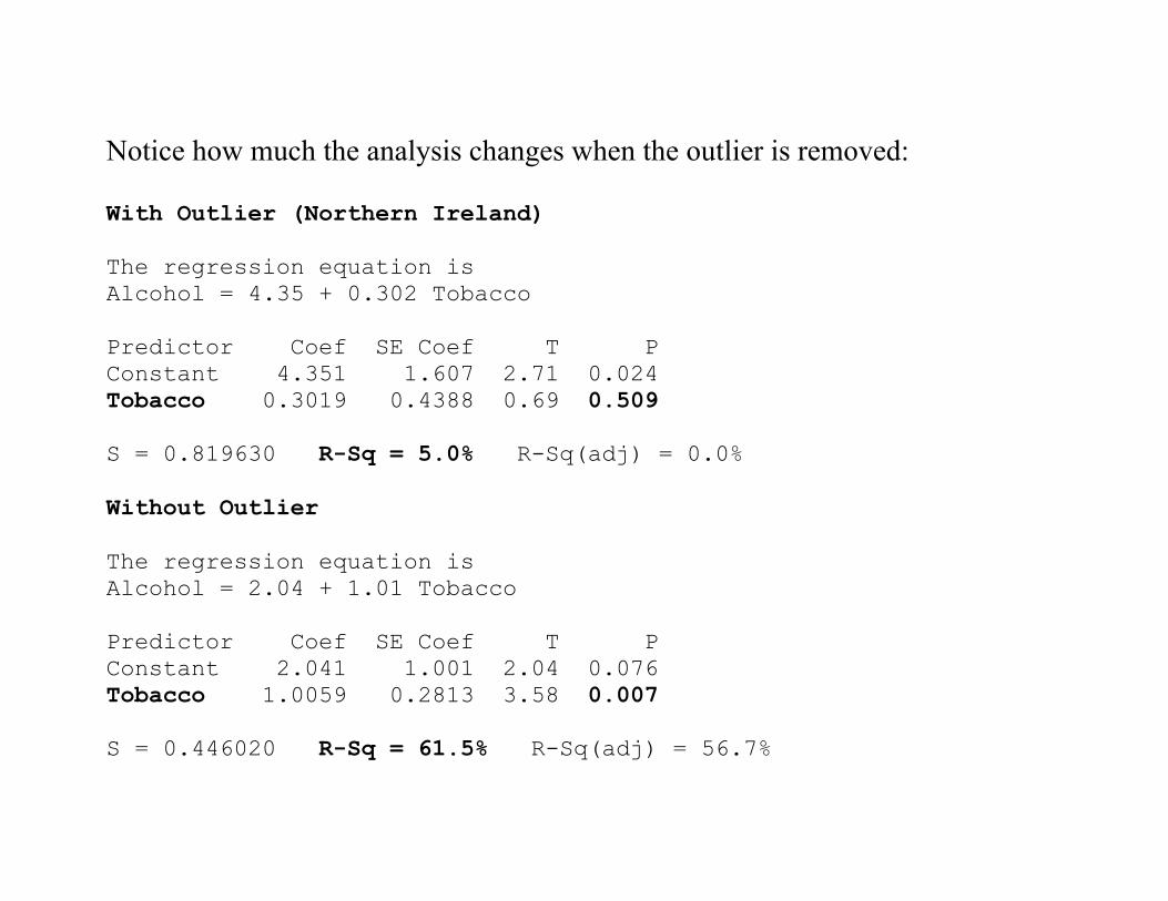
Notice how much the analysis changes when the outlier is removed: With Outlier (Northern Ireland) The regression equation is Alcohol = 4.35 + 0.302 Tobacco Predictor Coef SE Coef T P Constant 4.351 1.607 2.71 0.024 Tobacco 0.3019 0.4388 0.69 0.509 S = 0.819630 R-Sq = 5.0% R-Sq(adj) = 0.0% Without Outlier The regression equation is Alcohol = 2.04 + 1.01 Tobacco Predictor Coef SE Coef T P Constant 2.041 1.001 2.04 0.076 Tobacco 1.0059 0.2813 3.58 0.007 S = 0.446020 R-Sq = 61.5% R-Sq(adj) = 56.7%