Embed Size (px)
Citation preview

Association Analysis(chapter 6)
Professor Anita WasilewskaLecture Notes

Association Rules MiningAn Introduction
• This is an intuitive (more or less ) introduction• It contains explanation of the main ideas:• Frequent item sets, association rules, how we
construct the association rules,• how we judge the goodness of the rules• Example of an intuitive “run” of the Appriori
Algorithm and association rules generation• Discussion of the relationship between the
Association and Correlation analysis

What Is Association Mining?
Association rule mining:» Finding frequent patterns called
associations, among sets of items or objects in transaction databases, relational databases, and other information repositories.
• Applications:– Basket data analysis, cross-marketing, catalog design,
loss-leader analysis, clustering, classification, etc.

Association Rules
• Rule general form:“Body →Ηead [support, confidence]”
Rule Predicate form:buys(x, “diapers”) → buys(x, “beer”) [0.5%,
60%]major(x, “CS”) ^ takes(x, “DB”) → grade(x, “A”)
[1%, 75%]Rule Attribute form:Diapers → beer [1%, 75%]
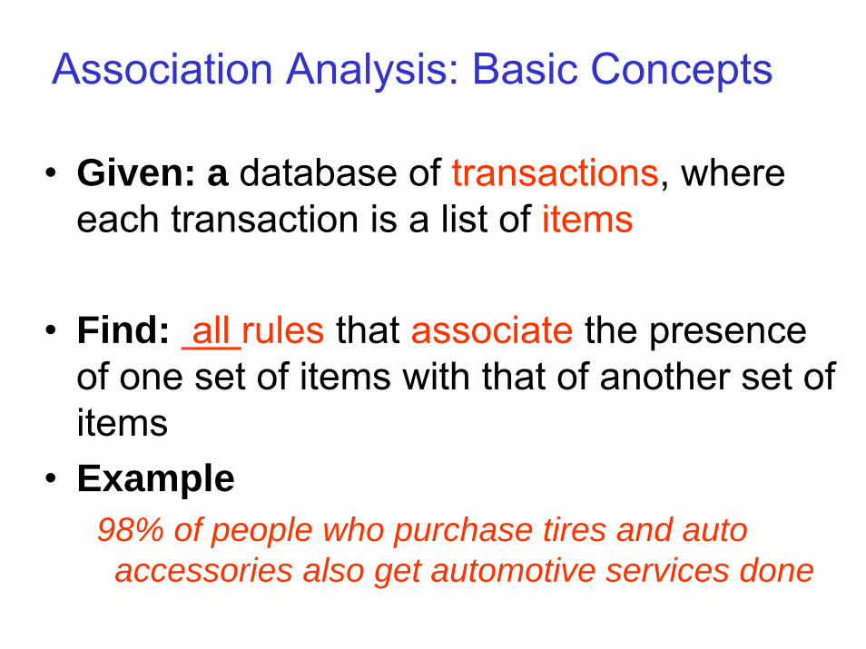
Association Analysis: Basic Concepts
• Given: a database of transactions, where each transaction is a list of items
• Find: all rules that associate the presence of one set of items with that of another set of items
• Example98% of people who purchase tires and auto accessories also get automotive services done

Association Model
• I ={i1, i2, ...., in} a set of items• J = P(I ) set of all subsets of the set of items,
elements of J are called itemsets• Transaction T: T is subset of set I of items• Data Base: set of transactions• An association rule is an implication of the
form : X-> Y, where X, Y are disjointsubsets of items I (elements of J )
• Problem: Find rules that have support andconfidence greater that user-specifiedminimum support and minimun confidence
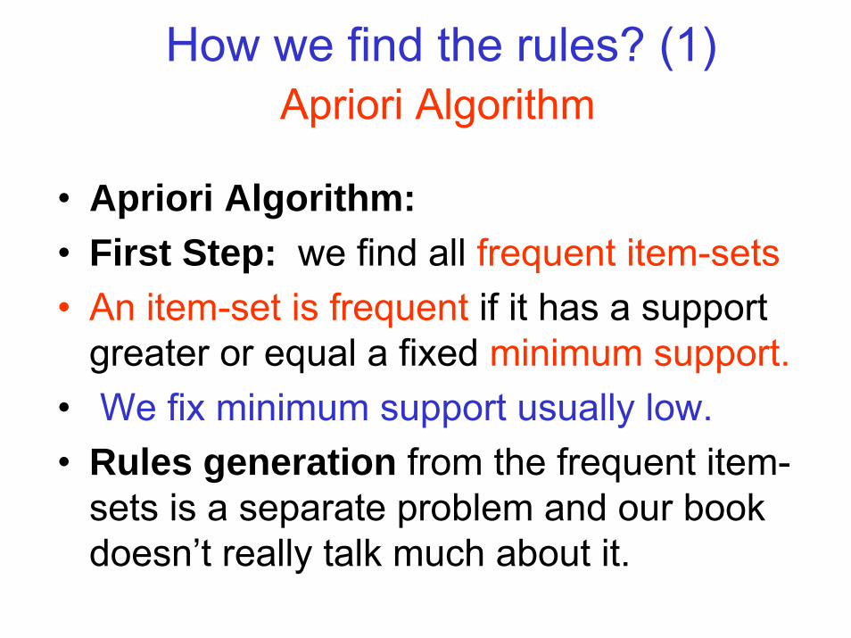
How we find the rules? (1) Apriori Algorithm
• Apriori Algorithm:• First Step: we find all frequent item-sets• An item-set is frequent if it has a support
greater or equal a fixed minimum support.• We fix minimum support usually low.• Rules generation from the frequent item-
sets is a separate problem and our book doesn’t really talk much about it.

How we find the rules? (2)Apriori Algorithm
• In order calculate efficiently frequent item-sets:• 1-item-sets (one element item-sets)• 2-item-sets (two elements item-sets)• 3-item-sets ( three elements item-sets)• etc….• we use a principle, called an Apriori Principle
(hence the name: Apriori Algorithm):• ANY SUBSET OF A FREQUENT ITEMSET IS
A FREQUENT ITEMSET

How we find the rules? (3) Apriori Process
• Appriori Algorithm stops after the First Step • Second Step in the Appriori Proces (item-sets
generarion AND rules generation) is the rule generation:
• We calculate, from the frequent item-sets a set of the strong rules .
• Strong rules: rules with at least minimum support (low) and minimum confidence (high)
• Apriori Process is then finished .

How we find the rules? (4)Apriori Process
• The Aprriori Process problem is:• how do we form the association rules
(A =>B) from the frequent item sets?• Remark: A, B are disjoint subsets of the
set I of items in general, and of the set 2-frequent, 3-frequent item sets ….. etc, …as generated by the Apriori Algorithm

How we find the rules? (5)
• 1-frequent item set: {i1}- no rule• 2-frequent item set {i1, i2}: there are two rules:• {i1} => {i2} and {i2} => {i2}• We write them also as• i1 => i2 and i2 => i2• We decide which rule we accept by calculating
its support (greater= minimum support) andconfidence (greater= minimum confidence)

How we find the rules? (6)
• 3-frequent item set: {i1, i2, i3}• The rules, by definition are of the form (A =>B) where
A and B are disjoint subsets of {i1, i2, i3}, i.e.• we have to find all subsets A,B of {i1, i2, i3} such that
A∪B = {i1, i2, i3} and A∩ B = Φ• For example,• let A= {i1, i2} and B= {i3}. The rule is • {i1, i2} => {i3}),• and we write it in a form:
( i1 ∩ i2 => i3 ) or milk ∩ bread => vodkaif item i1 is milk, item i2 is bread and item i3 is vodka

How we find the rules? (7)
• Another choice for A and B is, for example:• A= {i1} and B= {12, i3}.• The rule is• {i1} => {i2, i3}, and we write it in a form:
i1 => (i2∩ i3) or milk => (bread ∩ vodka)if item i1 is milk, item i2 is bread and item i3 is vodka
• REMEMBER:• We have to cover all the choices for A and B!• Which rule we accept is being decided by
calculating its support (greater = minimum support) and confidence (greater = minimum confidence)
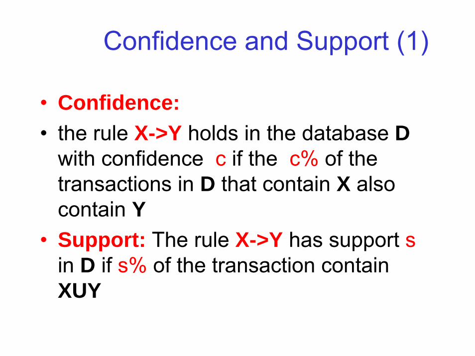
Confidence and Support (1)
• Confidence:• the rule X->Y holds in the database D
with confidence c if the c% of thetransactions in D that contain X alsocontain Y
• Support: The rule X->Y has support sin D if s% of the transaction containXUY
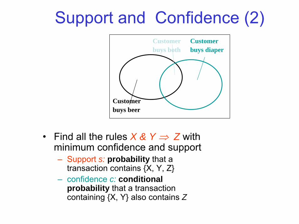
Support and Confidence (2)
• Find all the rules X & Y ⇒ Z with minimum confidence and support– Support s: probability that a
transaction contains {X, Y, Z}– confidence c: conditional
probability that a transaction containing {X, Y} also contains Z
Customerbuys diaper
Customerbuys both
Customerbuys beer

Support (definition)
• Support of a rule (A=>B) in the database D of transactions is given by formula (where sc=support count)
• Support( A => B) = P(A U B) =
sc(A U B)#D
Frequent Item sets: sets of items with a support support > MINIMAL supportWe (user) fix MIN support usually low and Min Confidence high

Confidence (definition)
• Confidence of a rule (A=>B) in the database D of transactions is given by formula (where sc=support count)
• Conf( A => B) = P(B|A) =
•=
=
P(A U B)P(A)
sc(AUB)#D
divided byscA#D
sc(AUB)scA
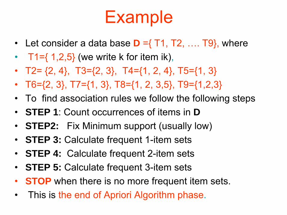
Example• Let consider a data base D ={ T1, T2, …. T9}, where• T1={ 1,2,5} (we write k for item ik),• T2= {2, 4}, T3={2, 3}, T4={1, 2, 4}, T5={1, 3}• T6={2, 3}, T7={1, 3}, T8={1, 2, 3,5}, T9={1,2,3}• To find association rules we follow the following steps• STEP 1: Count occurrences of items in D• STEP2: Fix Minimum support (usually low)• STEP 3: Calculate frequent 1-item sets• STEP 4: Calculate frequent 2-item sets• STEP 5: Calculate frequent 3-item sets• STOP when there is no more frequent item sets.• This is the end of Apriori Algorithm phase.

Example (c.d)• STEP 6: Fix the minimum confidence (usually
high)• STEP 7: Generate strong rules (support >min
support and confidence> min confidence)• END of rules generation phase.• Lets now calculate all steps of our process for
the data base D. We represent our transactional data base as relational data base (a table) and put the occurrences of items as an extra row, on the bottom (STEP 1)

Example (c.d)STEP 1: items occurrences=sc (in a table)
its 1 2 3 4 5T1 + + 0 0 +T2 0 + 0 + 0T3 0 + + 0 0T4 + + 0 + 0T5 + 0 + 0 0T6 0 + + 0 0T7 + 0 + 0 0T8 + + + 0 +T9 + + + 0 0sc 6 7 6 2 2

Example (c.d.)
• STEP 2: Fix minimal support count, for example
• msc = 2• Minimal support = msc/#D= 2/9=22%• ms=22%• Observe: minimal support of an item set is
determined uniquely by the minimal support count (msc) and we are going to use only mscto choose our frequent k-itemsets

Example (c.d.)• STEP 3: calculate frequent 1-item sets: look at the
count – we get that all 1-item sets are frequent.• STEP 4: calculate frequent 2-item sets.• First we calculate 2-item sets candidates from
frequent 1-item sets.• As our all 1-item sets are frequent so all subsets of any
2-item set are frequent and we have to find counts of all 2-item sets.
• If for example we set our msc=6, i.e we would have only {1}, {2} and {3} as frequent item sets then by Apriori Principle: “if A is a frequent item set, then each of its subsets is a frequent item set” we would be examining only those 2-item sets that have {1}, {2}, {3} as subsets
• Apriori Principle reduces the complexity of the algorithm

Example (c.d)• STEP 4 : All 2-item sets = all 2-element subsets of
{1,2,3,4,5,} are candidates and we evaluate theirsc=support counts (in red). They are called 2-item set candidates
• {1,2,} (4), {1,3} (4), {1,4} (1), {1,5} (2),• {2,3} (4), {2,4} (2), {2,5} ,• {3,4} (0), {3,5} (1),• {4,5} (0)• msc=2 and we get the folowing• Frequent 2- item sets: {1,2}, {1,3}, {1,5}, {2,3}, {2,4},
{2,5}

Example (c.d.)
• STEP 5: generate all frequent 3-item sets.• FIRST: use the frequent 2-item sets to generate
all 3-item set candidates.• SECOND: use Apriori Principle to prune the
candidates set• THIRD: Evaluate the count of the pruned set• STOP: list the frequent 3-item sets• STEP 6: repeat the procedure for 4-itemsets
etc (if any)

Example (c.d.)• STEP 5 (c.d): generate all frequent 3-item sets.
• FIRST: 3-item set candidates are: {1,2,3}, {1,2,4}, {1,2,5}, {1,3,4}, {1,3,5}, {2,3,4}, {2,3,5}, {2,4,5}
• SECOND: pruned the candidates set is:• {1,2,3}, {1,2,5}
• THIRD: the sc=support count of the pruned set is:• {1,2,3} (2), {1,2,5} (2)• STOP: list the frequent 3-item sets:• {1,2,3}, {1,2,5}• STEP 6: there is no 4-item sets.• STEP 7: Use the confidence to generate Apriori Rules.• We fix minimum confidence = 70%
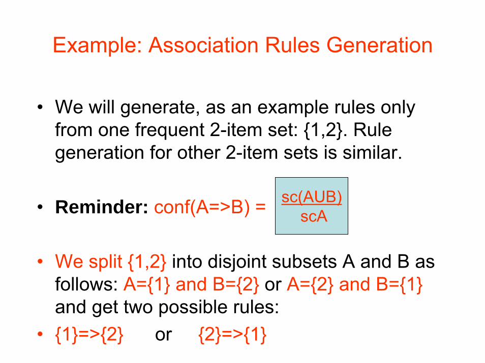
Example: Association Rules Generation
• We will generate, as an example rules only from one frequent 2-item set: {1,2}. Rule generation for other 2-item sets is similar.
• Reminder: conf(A=>B) =
• We split {1,2} into disjoint subsets A and B as follows: A={1} and B={2} or A={2} and B={1}and get two possible rules:
• {1}=>{2} or {2}=>{1}
sc(AUB)scA
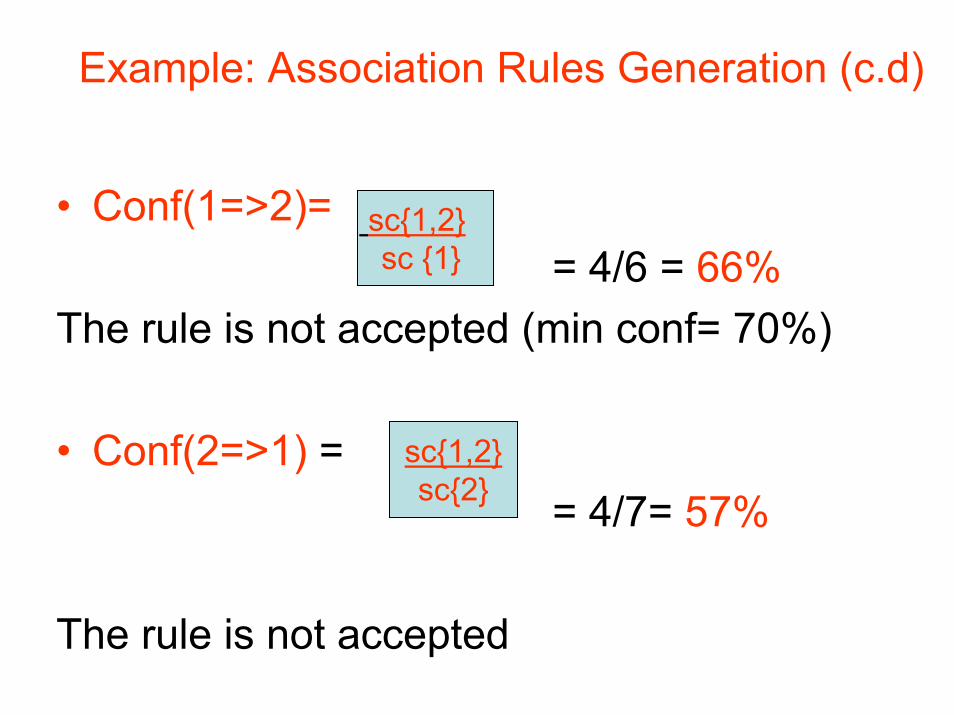
Example: Association Rules Generation (c.d)
• Conf(1=>2)== 4/6 = 66%
The rule is not accepted (min conf= 70%)
• Conf(2=>1) = = 4/7= 57%
The rule is not accepted
sc{1,2} sc {1}
sc{1,2}sc{2}

Example: Association Rules Generation (c.d.)
• Now we use one frequent 3-item set• {1,2,5} to show how to generate strong rules.• First we evaluate all possibilities how to split the
set {1,2,5} into to disjoint subsets A,B to obtain all possible rules (A=>B).
• For each rule we evaluate its confidence and choose only those with conf ≥ 70% (our minimal confidence).
• The minimal support condition is fulfilled as we deal only with frequent items.
• The rules such obtained are strong rules.
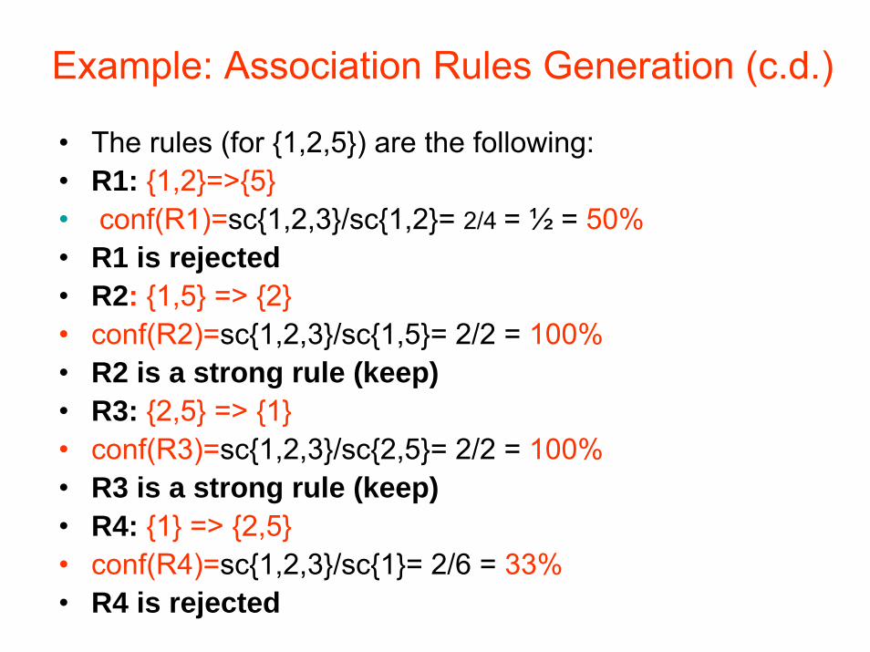
Example: Association Rules Generation (c.d.)
• The rules (for {1,2,5}) are the following:• R1: {1,2}=>{5}• conf(R1)=sc{1,2,3}/sc{1,2}= 2/4 = ½ = 50%• R1 is rejected• R2: {1,5} => {2}• conf(R2)=sc{1,2,3}/sc{1,5}= 2/2 = 100%• R2 is a strong rule (keep)• R3: {2,5} => {1}• conf(R3)=sc{1,2,3}/sc{2,5}= 2/2 = 100%• R3 is a strong rule (keep)• R4: {1} => {2,5}• conf(R4)=sc{1,2,3}/sc{1}= 2/6 = 33%• R4 is rejected

Example: Association Rules Generation (c.d.)
• The next rules (for {1,2,5}) are the following:• R5: {2}=>{1,5}• conf(R5)=sc{1,2,3}/sc{2}= 2/7 = 27%• R5 is rejected• R6: {5} => {1,2}• conf(R6)=sc{1,2,3}/sc{5}= 2/2 = 100%• R6 is a strong rule (keep)• As the last step we evaluate the exact support for the
strong rules (we know that already that it is greater or equal to minimum support, as rules were obtained from the frequent item sets)

Example: Association Rules Generation (c.d.)
• Exact support for the strong rules is:• Sup({1,5}=>{2})=sc{1,2,5}/#D=2/9= 22%• We write:• 1∩ 5 => 2 [22%, 100%]• Sup({2,5}=>{1}) =sc{1,2,5}/#D=2/9= 22%• We write:• 2∩ 5 => 1 [22%, 100%]• Sup({5}=>{1,2}) =sc{1,2,5}/#D=2/9= 22%• We write:• 5 => 1 ∩ 2 [22%, 100%]• THE END

Criticism to Support and Confidence
• Example 1: (Aggarwal & Yu, PODS98)– Among 5000 students
• 3000 play basketball• 3750 eat cereal• 2000 both play basket ball and eat cereal
RULE: play basketball ⇒ eat cereal [40%, 66.7%] is misleading because the overall percentage of students eating cereal is 75% which is higher than 66.7%.
RULE: play basketball ⇒ not eat cereal [20%, 33.3%] is far more accurate, although with lower support and confidence
basketball not basketball sum(row)cereal 2000 1750 3750not cereal 1000 250 1250sum(col.) 3000 2000 5000

Association and Correlation
• As we can see support-confidence framework can be misleading;
• it can identify a rule (A=>B) as interesting (strong) when, in fact the occurrence of A might not imply the occurrence of B.
• Correlation Analysis provides an alternative framework for finding interesting relationships,
• or to improve understanding of meaning of some association rules (a lift of an association rule)
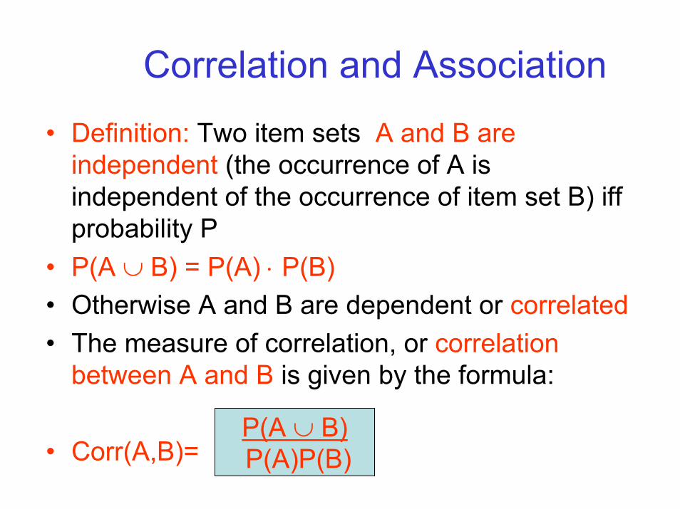
Correlation and Association
• Definition: Two item sets A and B are independent (the occurrence of A is independent of the occurrence of item set B) iffprobability P
• P(A ∪ B) = P(A) ⋅ P(B)• Otherwise A and B are dependent or correlated• The measure of correlation, or correlation
between A and B is given by the formula:
• Corr(A,B)=P(A ∪ B)P(A)P(B)
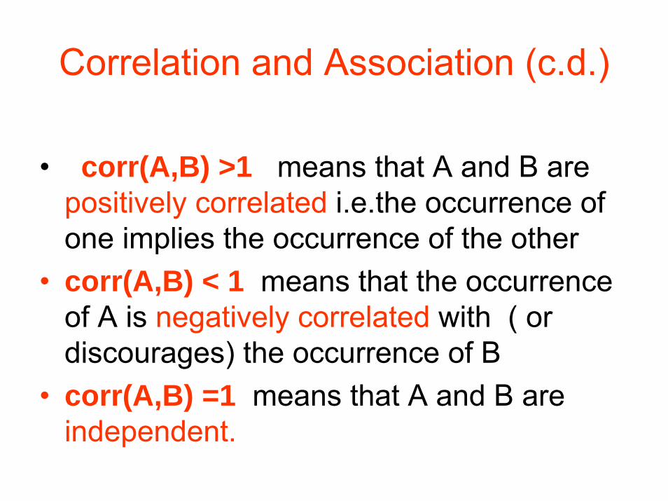
Correlation and Association (c.d.)
• corr(A,B) >1 means that A and B arepositively correlated i.e.the occurrence of one implies the occurrence of the other
• corr(A,B) < 1 means that the occurrence of A is negatively correlated with ( or discourages) the occurrence of B
• corr(A,B) =1 means that A and B are independent.
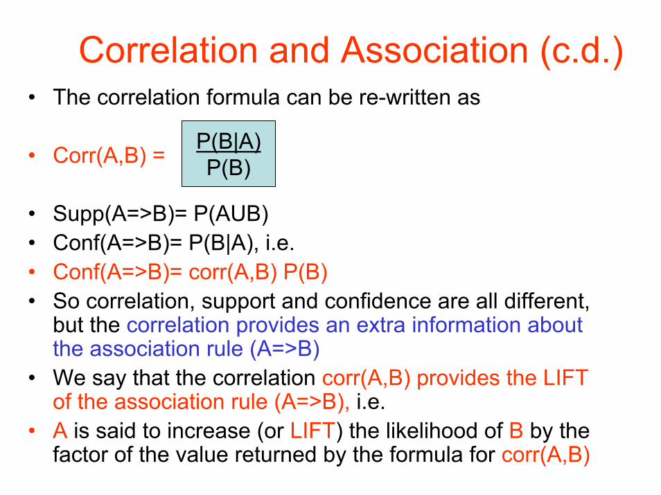
Correlation and Association (c.d.)• The correlation formula can be re-written as
• Corr(A,B) =
• Supp(A=>B)= P(AUB)• Conf(A=>B)= P(B|A), i.e.• Conf(A=>B)= corr(A,B) P(B)• So correlation, support and confidence are all different,
but the correlation provides an extra information about the association rule (A=>B)
• We say that the correlation corr(A,B) provides the LIFT of the association rule (A=>B), i.e.
• A is said to increase (or LIFT) the likelihood of B by the factor of the value returned by the formula for corr(A,B)
P(B|A)P(B)

Correlation Rules
• A correlation rule is a set of items• {i1, i2, ….in}, where the items occurrences are
correlated. • The correlation value is given by the correlation formula
and we use Χ square test to determine if correlation is statistically significant.
• The Χ square test can also determine the negative correlation.We can also form minimal correlated item sets, etc…
• Limitations: Χ square test is less accurate on the data tables that are sparse and can be misleading for the contingency tables larger then 2x2
Mining Association Rules in Large Databases (Chapter 6)
• Association rule mining• Mining single-dimensional Boolean association rules
from transactional databases• Mining multilevel association rules from transactional
databases• Mining multidimensional association rules from
transactional databases and data warehouse• From association mining to correlation analysis• Constraint-based association mining• Summary
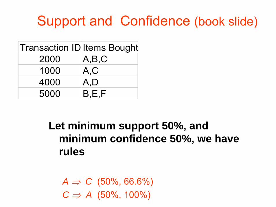
Support and Confidence (book slide)
Transaction ID Items Bought2000 A,B,C1000 A,C4000 A,D5000 B,E,F
Let minimum support 50%, and minimum confidence 50%, we have rules
A ⇒ C (50%, 66.6%)C ⇒ A (50%, 100%)

Association Rule Mining: A Road Map
• Boolean (Qualitative) vs. quantitative associations (Based on the types of values handled)
buys(x, “SQLServer”) ^ income(x, “DMBook”) => buys(x, “DBMiner”) [0.2%, 60%] (Boolean/Qualitative)
age(x, “30..39”) ^ income(x, “42..48K”) => buys(x, “PC”) [1%, 75%](quantitative)
• Single dimension (one predicate) vs. multiple dimensional associations (multiple predicates )

Association Rule Road Map (c.d)
• Single level vs. multiple-level analysis– What brands of beers are associated with what brands
of diapers – single level– Various extensions1. Correlation analysis (just discussed)2. Association does not necessarily imply correlation or
causality3. Constraints enforced
Example:
smallsales (sum < 100) implies bigbuys (sum >1,000)?

Chapter 6: Mining Association Rules
• Association rule mining• Mining single-dimensional Boolean association rules
from transactional databases• Mining multilevel association rules from transactional
databases• Mining multidimensional association rules from
transactional databases and data warehouse• From association mining to correlation analysis• Constraint-based association mining• Summary
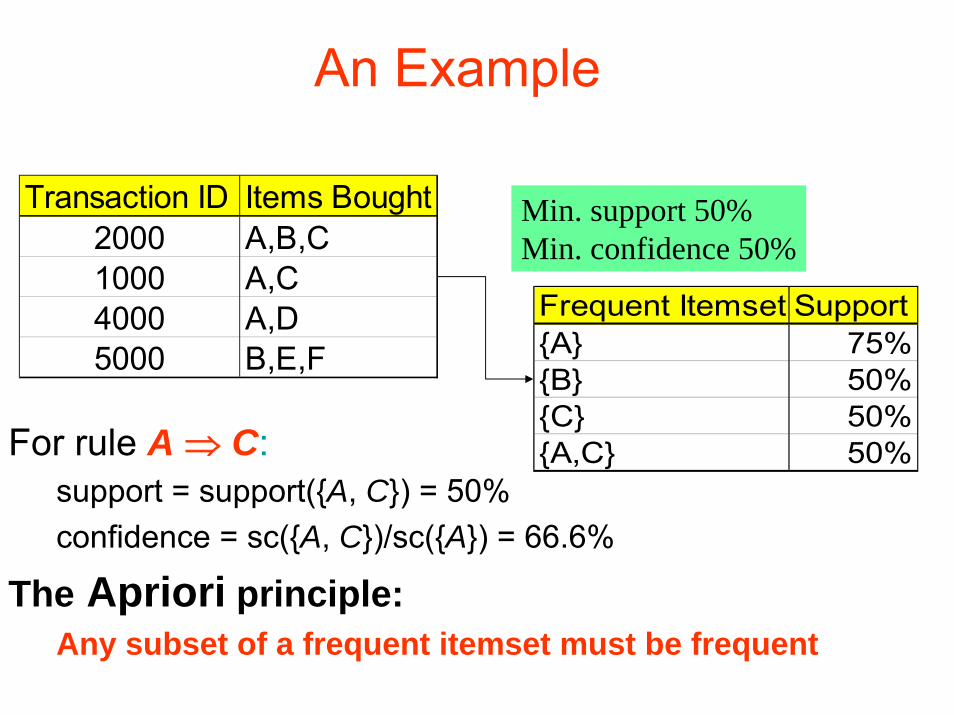
An Example
For rule A ⇒ C:support = support({A, C}) = 50%confidence = sc({A, C})/sc({A}) = 66.6%
The Apriori principle:Any subset of a frequent itemset must be frequent
Transaction ID Items Bought2000 A,B,C1000 A,C4000 A,D5000 B,E,F
Frequent Itemset Support{A} 75%{B} 50%{C} 50%{A,C} 50%
Min. support 50%Min. confidence 50%
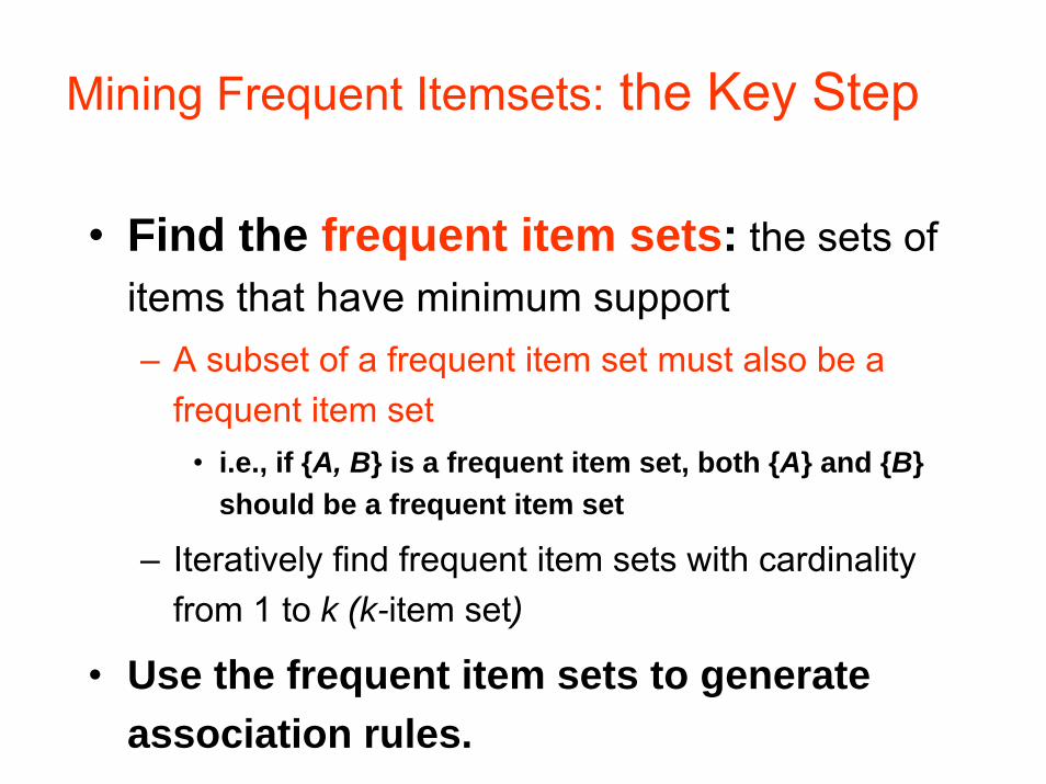
Mining Frequent Itemsets: the Key Step
• Find the frequent item sets: the sets of items that have minimum support– A subset of a frequent item set must also be a
frequent item set• i.e., if {A, B} is a frequent item set, both {A} and {B}
should be a frequent item set
– Iteratively find frequent item sets with cardinality from 1 to k (k-item set)
• Use the frequent item sets to generate association rules.

Apriori Algorithm — Book Example of frequents items sets generation
TID Items100 1 3 4200 2 3 5300 1 2 3 5400 2 5
Database D itemset sup.{1} 2{2} 3{3} 3{4} 1{5} 3
itemset sup.{1} 2{2} 3{3} 3{5} 3
Scan D
C1L1
itemset{1 2}{1 3}{1 5}{2 3}{2 5}{3 5}
itemset sup{1 2} 1{1 3} 2{1 5} 1{2 3} 2{2 5} 3{3 5} 2
itemset sup{1 3} 2{2 3} 2{2 5} 3{3 5} 2
L2
C2 C2Scan D
C3 L3itemset{2 3 5}
Scan D itemset sup{2 3 5} 2

The Apriori Algorithm (Book)
• Pseudo-code:Ck: Candidate itemset of size kLk : frequent itemset of size k
L1 = {frequent items};for (k = 1; Lk !=∅; k++) do begin
Ck+1 = candidates generated from Lk;for each transaction t in database do
increment the count of all candidates in Ck+1that are contained in t
Lk+1 = candidates in Ck+1 with min_supportend
return ∪k Lk;

Generating Candidates: Ck
• Join Step: Ck is generated by joining Lk-with itself
• Prune Step: Any (k-1)-item set that is not frequent cannot be a subset of a frequent k-item set

Example of Generating Candidates
• L3={abc, abd, acd, ace, bcd}
• We write abc for {a,b,c}, etc…
• Self-joining: L3*L3
– abcd from abc and abd
– acde from acd and ace
• Pruning:– acde is removed because ade is not frequent: is not in L3
• C4={abcd}
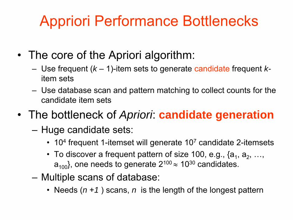
Appriori Performance Bottlenecks
• The core of the Apriori algorithm:– Use frequent (k – 1)-item sets to generate candidate frequent k-
item sets– Use database scan and pattern matching to collect counts for the
candidate item sets
• The bottleneck of Apriori: candidate generation– Huge candidate sets:
• 104 frequent 1-itemset will generate 107 candidate 2-itemsets• To discover a frequent pattern of size 100, e.g., {a1, a2, …,
a100}, one needs to generate 2100 ≈ 1030 candidates.– Multiple scans of database:
• Needs (n +1 ) scans, n is the length of the longest pattern

How to Count Supports of Candidates?
• Why counting supports of candidates is a problem?– The total number of candidates can be very huge– One transaction may contain many candidates
• Method:– Candidate itemsets are stored in a hash-tree– Leaf node of hash-tree contains a list of itemsets and counts– Interior node contains a hash table– Subset function: finds all the candidates contained in a
transaction

Methods to Improve Apriori’s Efficiency
• Hash-based itemset counting: A k-itemset whose
corresponding hashing bucket count is below the
threshold cannot be frequent
• Transaction reduction: A transaction that does not
contain any frequent k-itemset is useless in subsequent
scans
• Partitioning: Any itemset that is potentially frequent in
DB must be frequent in at least one of the partitions of
DB
• Sampling: mining on a subset of given data lower

An Alternative: Mining Frequent Patterns Without Candidate Generation
• Compress a large database into a compact, Frequent-Pattern tree (FP-tree) structure– highly condensed, but complete for frequent pattern mining– avoid costly database scans
• Develop an efficient, FP-tree-based frequent pattern mining method– A divide-and-conquer methodology: decompose
mining tasks into smaller ones– Avoid candidate generation: sub-database test only!

Why Is Frequent Pattern Growth Fast?
• Performance study shows– FP-growth is an order of magnitude faster than
Apriori, and is also faster than tree-projection
• Reasoning– No candidate generation, no candidate test
– Use compact data structure
– Eliminate repeated database scan
– Basic operation is counting and FP-tree building

FP-growth vs. Apriori: Scalability With the Support Threshold
0
10
20
30
40
50
60
70
80
90
100
0 0.5 1 1.5 2 2.5 3Support threshold(%)
Run
tim
e(se
c.)
D1 FP-grow th runtime
D1 Apriori runtime
Data set T25I20D10K

FP-growth vs. Tree-Projection: Scalability with Support Threshold
0
20
40
60
80
100
120
140
0 0.5 1 1.5 2
Support threshold (%)
Runt
ime
(sec
.)
D2 FP-growthD2 TreeProjection
Data set T25I20D100K

Presentation of Association Rules(Table Form )

Visualization of Association Rule Using Plane Graph

Visualization of Association Rule Using Rule Graph
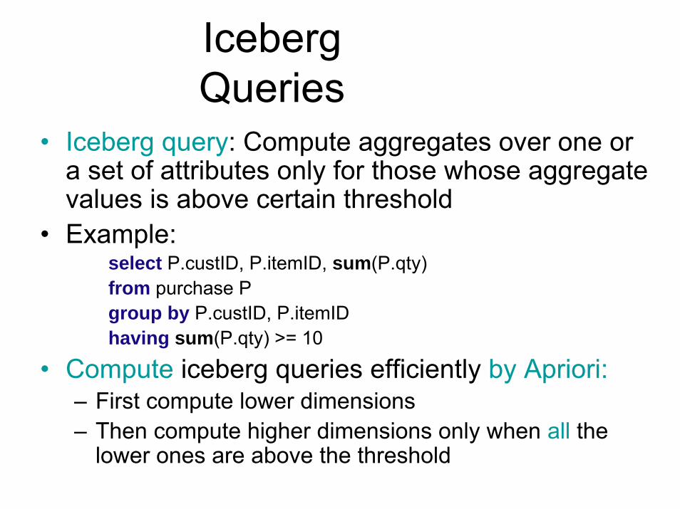
Iceberg Queries
• Iceberg query: Compute aggregates over one or a set of attributes only for those whose aggregate values is above certain threshold
• Example:select P.custID, P.itemID, sum(P.qty)from purchase Pgroup by P.custID, P.itemIDhaving sum(P.qty) >= 10
• Compute iceberg queries efficiently by Apriori:– First compute lower dimensions– Then compute higher dimensions only when all the
lower ones are above the threshold
Chapter 6: Mining Association Rules in Large Databases
• Association rule mining• Mining single-dimensional Boolean association
rules from transactional databases• Mining multilevel association rules from
transactional databases• Mining multidimensional association rules from
transactional databases and data warehouse• From association mining to correlation
analysis• Constraint-based association mining

Multiple-Level Association Rules
• Items often form hierarchy
• Items at the lower level are expected to have lower support.
• Rules regarding itemsetsatappropriate levels could be quite useful.
• Transaction database can be encoded based
di i d l l
Food
breadmilk
skim
SunsetFraser
2% whitewheat
TID ItemsT1 {111, 121, 211, 221}T2 {111, 211, 222, 323}T3 {112, 122, 221, 411}T4 {111, 121}T5 {111, 122, 211, 221, 413}

Mining Multi-Level Associations
• A top_down, progressive deepening approach:– First find high-level strong rules:
milk → bread [20%, 60%].– Then find their lower-level “weaker” rules:
2% milk → wheat bread [6%, 50%].• Variations at mining multiple-level
association rules.– Level-crossed association rules:
2% milk → Wonder wheat bread– Association rules with multiple, alternative
hierarchies:2% milk → Wonder bread

Chapter 6: Mining Association Rules in
Large Databases• Association rule mining• Mining single-dimensional Boolean association
rules from transactional databases• Mining multilevel association rules from
transactional databases• Mining multidimensional association rules from
transactional databases and data warehouse• From association mining to correlation
analysis• Constraint-based association mining

Multi-Dimensional Association (1)
• Single-dimensional rules:
– buys(X, “milk”) ⇒ buys(X, “bread”)
• Multi-dimensional rules: Involve 2 or more dimensions or predicates
– Inter-dimension association rules (no repeated predicates)
• age(X,”19-25”) ∧occupation(X,“student”) ⇒buys(X,“coke”)

Multi-Dimensional Association
– Hybrid-dimension association rules (repeated predicates)
• age(X,”19-25”) ∧ buys(X, “popcorn”) ⇒buys(X, “coke”)
• Categorical (qualitative) Attributes– finite number of possible values, no
ordering among values• Quantitative Attributes
– numeric, implicit ordering among values

Techniques for Mining MD Associations
• Search for frequent k-predicate set:– Example: {age, occupation, buys} is a 3-predicate set.– Techniques can be categorized by how age are treated.
1. Using static discretization of quantitative attributes– Quantitative attributes are statically discretized by using
predefined concept hierarchies.2. Quantitative association rules
– Quantitative attributes are dynamically discretized into “bins”based on the distribution of the data.
3. Distance-based association rules– This is a dynamic discretization process that considers the
distance between data points.

Static Discretization of Quantitative Attributes
• Discretized prior to mining using concept hierarchy.
• Numeric values are replaced by ranges.• In relational database, finding all frequent k-
predicate sets will require k or k+1 table scans.• Data cube is well suited for mining.• The cells of an n-dimensional
cuboid correspond to the predicate sets.
• Mining from data cubescan be much faster.
(income)(age)
()
(buys)
(age, income) (age,buys) (income,buys)
(age,income,buys)
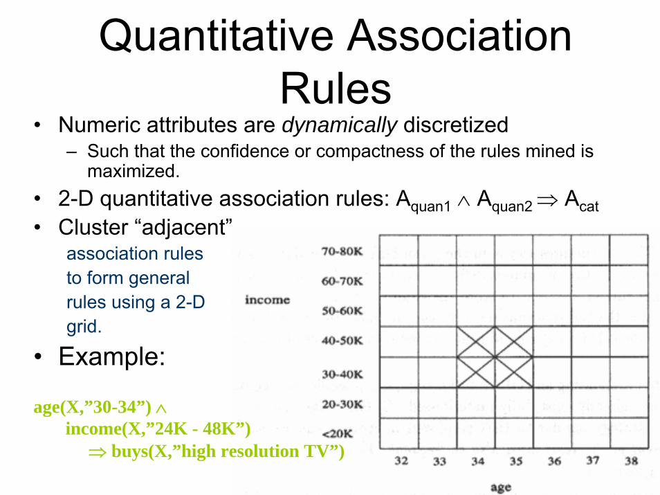
Quantitative Association Rules
age(X,”30-34”) ∧income(X,”24K - 48K”)
⇒ buys(X,”high resolution TV”)
• Numeric attributes are dynamically discretized– Such that the confidence or compactness of the rules mined is
maximized.• 2-D quantitative association rules: Aquan1 ∧ Aquan2 ⇒ Acat• Cluster “adjacent”
association rulesto form general rules using a 2-D grid.
• Example:

ARCS (Association Rule Clustering System)
1. Binning
2. Find frequent predicateset
3. Clustering
4. Optimize
How does ARCS work?

Limitations of ARCS
• Only quantitative attributes on LHS of rules.
• Only 2 attributes on LHS. (2D limitation)
• An alternative to ARCS– Non-grid-based
– equi-depth binning
– clustering based on a measure of partial completeness.
– “Mining Quantitative Association Rules in Large Relational Tables” by R. Srikant and R. Agrawal.

Mining Distance-based Association Rules
• Binning methods do not capture the semantics of interval data
• Distance-based partitioning, more meaningful discretizationconsidering:– density/number of points in an interval– “closeness” of points in an interval
Price($)Equi-width(width $10)
Equi-depth(depth 2)
Distance-based
7 [0,10] [7,20] [7,7]20 [11,20] [22,50] [20,22]22 [21,30] [51,53] [50,53]50 [31,40]51 [41,50]53 [51,60]

• S[X] is a set of N tuples t1, t2, …, tN , projected on the attribute set X
• The diameter of S[X]:
– distx:distance metric, e.g. Euclidean distance or
Manhattan
)1(
])[],[(])[( 1 1
−=∑ ∑= =
NN
XtXtdistXSd
jiN
i
N
jX
Clusters and Distance Measurements

• The diameter, d, assesses the density of a cluster CX , where
• Finding clusters and distance-based rules– the density threshold, d0 , replaces the notion of support– modified version of the BIRCH clustering algorithm
XdCd X 0)( ≤
0sCX ≥
Clusters and Distance Measurements(c.d.)
Chapter 6: Mining Association Rules in
Large Databases• Association rule mining• Mining single-dimensional Boolean association
rules from transactional databases• Mining multilevel association rules from
transactional databases• Mining multidimensional association rules from
transactional databases and data warehouse• From association mining to correlation
analysis• Constraint-based association mining
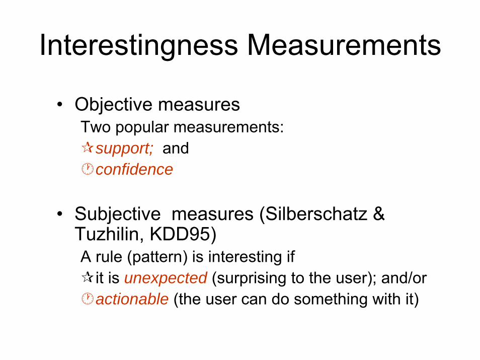
Interestingness Measurements
• Objective measuresTwo popular measurements:
support; and confidence
• Subjective measures (Silberschatz & Tuzhilin, KDD95)A rule (pattern) is interesting if
it is unexpected (surprising to the user); and/oractionable (the user can do something with it)

Criticism to Support and Confidence (Cont.)
• Example 2:– X and Y: positively correlated,– X and Z, negatively related– support and confidence of
X=>Z dominates
X 1 1 1 1 0 0 0 0Y 1 1 0 0 0 0 0 0Z 0 1 1 1 1 1 1 1
Rule Support ConfidenceX=>Y 25% 50%X=>Z 37.50% 75%
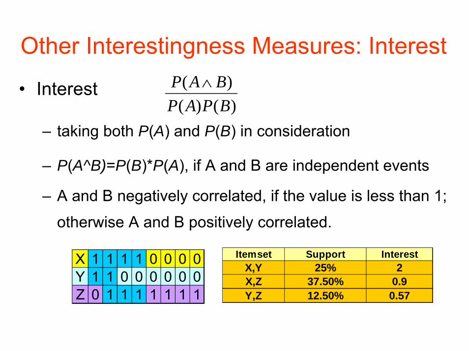
Other Interestingness Measures: Interest
• Interest
– taking both P(A) and P(B) in consideration
– P(A^B)=P(B)*P(A), if A and B are independent events
– A and B negatively correlated, if the value is less than 1;
otherwise A and B positively correlated.
)()()(
BPAPBAP ∧
X 1 1 1 1 0 0 0 0Y 1 1 0 0 0 0 0 0Z 0 1 1 1 1 1 1 1
Itemset Support InterestX,Y 25% 2X,Z 37.50% 0.9Y,Z 12.50% 0.57

Chapter 6: Mining Association Rules in Large Databases
• Association rule mining• Mining single-dimensional Boolean association rules
from transactional databases• Mining multilevel association rules from transactional
databases• Mining multidimensional association rules from
transactional databases and data warehouse• From association mining to correlation analysis• Constraint-based association mining• Summary
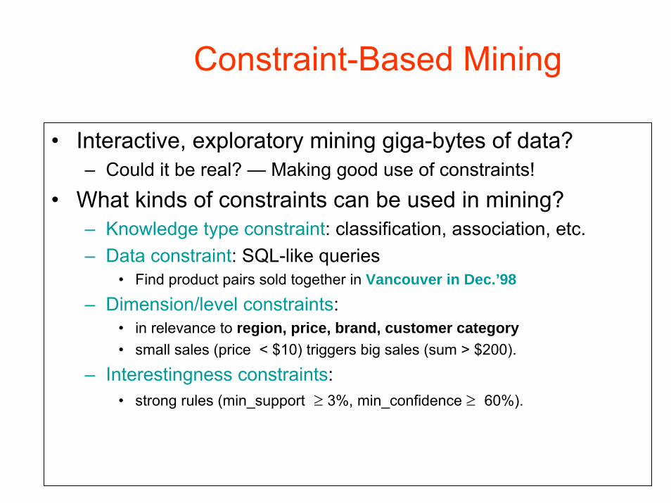
Constraint-Based Mining
• Interactive, exploratory mining giga-bytes of data? – Could it be real? — Making good use of constraints!
• What kinds of constraints can be used in mining?– Knowledge type constraint: classification, association, etc.– Data constraint: SQL-like queries
• Find product pairs sold together in Vancouver in Dec.’98
– Dimension/level constraints:• in relevance to region, price, brand, customer category• small sales (price < $10) triggers big sales (sum > $200).
– Interestingness constraints:• strong rules (min_support ≥ 3%, min_confidence ≥ 60%).

Rule Constraints in Association Mining
• Two kind of rule constraints:– Rule form constraints: meta-rule guided mining.
• P(x, y) ^ Q(x, w) → takes(x, “database systems”).
– Rule (content) constraint: constraint-based query optimization (Ng, et al., SIGMOD’98).
• sum(LHS) < 100 ^ min(LHS) > 20 ^ count(LHS) > 3 ^ sum(RHS) > 1000
• 1-variable vs. 2-variable constraints (Lakshmanan, et al. SIGMOD’99): – 1-var: A constraint confining only one side (L/R) of the
rule, e.g., as shown above. – 2-var: A constraint confining both sides (L and R).
• sum(LHS) < min(RHS) ^ max(RHS) < 5* sum(LHS)
Chapter 6: Mining Association Rules in Large Databases
• Association rule mining• Mining single-dimensional Boolean association rules
from transactional databases• Mining multilevel association rules from transactional
databases• Mining multidimensional association rules from
transactional databases and data warehouse• From association mining to correlation analysis• Constraint-based association mining• Summary

Why Is the Big Pie Still There?
• More on constraint-based mining of associations– Boolean vs. quantitative associations
• Association on discrete vs. continuous data– From association to correlation and causal structure
analysis.• Association does not necessarily imply correlation or causal
relationships– From intra-trasanction association to inter-
transaction associations• E.g., break the barriers of transactions (Lu, et al. TOIS’99).
– From association analysis to classification and clustering analysis
• E.g, clustering association rules
Summary
• Association rule mining– probably the most significant contribution from the
database community in KDD– A large number of papers have been published
• Many interesting issues have been explored• An interesting research direction
– Association analysis in other types of data: spatial data, multimedia data, time series data, etc.