ASSIGNMENT CLASSIFICATION TABLE (BY TOPIC)ftp.oz.nthu.edu.tw/~g9771501/isv_sm_ch06.pdf · Accounting Measurements, ... 6-5 CE6-2 (Continued) 50-1 The changes in the carrying amount

Copyright © 2010 John Wiley & Sons, Inc. Kieso, Intermediate Accounting, 13/e, Solutions Manual (For Instructor Use Only) 6-1

CHAPTER 6

Accounting and the Time Value of Money ASSIGNMENT CLASSIFICATION TABLE (BY TOPIC) Topics

Questions

Brief Exercises

Exercises

Problems

1. Present value concepts. 1, 2, 3, 4, 5, 9, 17

2. Use of tables. 13, 14 8 1

3. Present and future value problems:

a. Unknown future amount. 7, 19 1, 5, 13 2, 3, 4, 7

b. Unknown payments. 10, 11, 12 6, 12, 15, 17 8, 16, 17 2, 6

c. Unknown number of periods.

4, 9 10, 15 2

d. Unknown interest rate. 15, 18 3, 11, 16 9, 10, 11, 14 2, 7

e. Unknown present value. 8, 19 2, 7, 8, 10, 14 3, 4, 5, 6, 8, 12, 17, 18, 19

1, 4, 7, 9, 13, 14

4. Value of a series of irregular deposits; changing interest rates.

3, 5, 8

5. Valuation of leases, pensions, bonds; choice between projects.

6 15 7, 12, 13, 14, 15

3, 5, 6, 8, 9, 10, 11, 12, 13, 14, 15

6. Deferred annuity. 16

7. Expected Cash Flows. 20, 21, 22 13, 14, 15

6-2 Copyright © 2010 John Wiley & Sons, Inc. Kieso, Intermediate Accounting, 13/e, Solutions Manual (For Instructor Use Only)

ASSIGNMENT CLASSIFICATION TABLE (BY LEARNING OBJECTIVE) Learning Objectives

Brief Exercises

Exercises

Problems

1. Identify accounting topics where the time value of money is relevant.

2. Distinguish between simple and compound interest.

2

3. Use appropriate compound interest tables. 1

4. Identify variables fundamental to solving interest problems.

5. Solve future and present value of 1 problems. 1, 2, 3, 4, 7, 8

2, 3, 6, 9, 10, 15

1, 2, 3, 5, 7, 9, 10

6. Solve future value of ordinary and annuity due problems.

5, 6, 9, 13 3, 4, 6, 15, 16

2, 7

7. Solve present value of ordinary and annuity due problems.

10, 11, 12, 14, 16, 17

3, 4, 5, 6, 11, 12, 17, 18, 19

1, 2, 3, 4, 5, 7, 8, 9, 10, 13, 14

8. Solve present value problems related to deferred annuities and bonds.

15 7, 8, 13, 14 5, 6, 11, 12, 15

9. Apply expected cash flows to present value measurement.

20, 21, 22 13, 14, 15


ASSIGNMENT CHARACTERISTICS TABLE Item

Description

Level of Difficulty

Time (minutes)

E6-1 Using interest tables. Simple 5–10 E6-2 Simple and compound interest computations. Simple 5–10 E6-3 Computation of future values and present values. Simple 10–15 E6-4 Computation of future values and present values. Moderate 15–20 E6-5 Computation of present value. Simple 10–15 E6-6 Future value and present value problems. Moderate 15–20 E6-7 Computation of bond prices. Moderate 12–17 E6-8 Computations for a retirement fund. Simple 10–15 E6-9 Unknown rate. Moderate 5–10 E6-10 Unknown periods and unknown interest rate. Simple 10–15 E6-11 Evaluation of purchase options. Moderate 10–15 E6-12 Analysis of alternatives. Simple 10–15 E6-13 Computation of bond liability. Moderate 15–20 E6-14 Computation of pension liability. Moderate 15–20 E6-15 Investment decision. Moderate 15–20 E6-16 Retirement of debt. Simple 10–15 E6-17 Computation of amount of rentals. Simple 10–15 E6-18 Least costly payoff. Simple 10–15 E6-19 Least costly payoff—annuity due. Simple 10–15 E6-20 Expected cash flows. Simple 5–10 E6-21 Expected cash flows and present value. Moderate 15–20 E6-22 Fair value estimate. Moderate 15–20 P6-1 Various time value situations. Moderate 15–20 P6-2 Various time value situations. Moderate 15–20 P6-3 Analysis of alternatives. Moderate 20–30 P6-4 Evaluating payment alternatives. Moderate 20–30 P6-5 Analysis of alternatives. Moderate 20–25 P6-6 Purchase price of a business. Moderate 25–30 P6-7 Time value concepts applied to solve business problems. Complex 30–35 P6-8 Analysis of alternatives. Moderate 20–30 P6-9 Analysis of business problems. Complex 30–35 P6-10 Analysis of lease vs. purchase. Complex 30–35 P6-11 Pension funding. Complex 25–30 P6-12 Pension funding. Moderate 20–25 P6-13 Expected cash flows and present value. Moderate 20–25 P6-14 Expected cash flows and present value. Moderate 20–25 P6-15 Fair value estimate. Complex 20–25


SOLUTIONS TO CODIFICATION EXERCISES

CE6-1 (a) According to the Master Glossary, present value is a tool used to link uncertain future amounts

(cash flows or values) to a present amount using a discount rate (an application of the income approach) that is consistent with value maximizing behavior and capital market equilibrium. Present value techniques differ in how they adjust for risk and in the type of cash flows they use.

(b) The discount rate adjustment technique is a present value technique that uses a risk-adjusted

discount rate and contractual, promised, or most likely cash flows. (c) Other codification references to present value are at (1) FASB ASC 820-10-35-33 and (2) FASB

ASC 820-10-55-55-4. Details for these references follow.

1. 820 Fair Value Measurements and Disclosures > 10 Overall > 35 Subsequent Measurement

35-33 Those valuation techniques include the following:

a. Present value techniques

b. Option-pricing models (which incorporate present value techniques), such as the Black-Scholes-Merton formula (a closed-form model) and a binomial model (a lattice model)

c. The multiperiod excess earnings method, which is used to measure the fair value of

certain intangible assets.

2. 820 Fair Value Measurements and Disclosures > 10 Overall > 55 Implementation General, paragraph 55-4 >>> Present Value Techniques

55-4 FASB Concepts Statement No. 7, Using Cash Flow Information and Present Value in

Accounting Measurements, provides guidance for using present value techniques to measure fair value. That guidance focuses on a traditional or discount rate adjustment technique and an expected cash flow (expected present value) technique. This Section clarifies that guidance. (That guidance is included or otherwise referred to principally in paragraphs 39–46, 51, 62–71, 114, and 115 of Concepts Statement 7.) This Section neither prescribes the use of one specific present value technique nor limits the use of present value techniques to measure fair value to the techniques discussed herein. The present value technique used to measure fair value will depend on facts and cir-cumstances specific to the asset or liability being measured (for example, whether comparable assets or liabilities can be observed in the market) and the availability of sufficient data.

CE6-2 Answers will vary. By entering the phrase “present value” in the search window, a list of references to the term is provided. The site allows you to narrow the search to assets, liabilities, revenues, and expenses. (a) Asset reference: 350 Intangibles—Goodwill and Other > 20 Goodwill > 50 Disclosure > Goodwill

Impairment Loss > Information for Each Period for Which a Statement of Financial Position Is Presented


CE6-2 (Continued) 50-1 The changes in the carrying amount of goodwill during the period shall be disclosed, including

the following (see Example 3 [paragraph 350-20-55-24]): a. The aggregate amount of goodwill acquired. b. The aggregate amount of impairment losses recognized. c. The amount of goodwill included in the gain or loss on disposal of all or a portion of a

reporting unit. Entities that report segment information in accordance with Topic 280 shall provide the

above information about goodwill in total and for each reportable segment and shall disclose any significant changes in the allocation of goodwill by reportable segment. If any portion of goodwill has not yet been allocated to a reporting unit at the date the financial statements are issued, that unallocated amount and the reasons for not allocating that amount shall be disclosed.

> Goodwill Impairment Loss 50-2 For each goodwill impairment loss recognized, all of the following information shall be dis-

closed in the notes to the financial statements that include the period in which the impair-ment loss is recognized: a. A description of the facts and circumstances leading to the impairment. b. The amount of the impairment loss and the method of determining the fair value of the

associated reporting unit (whether based on quoted market prices, prices of comparable businesses, a present value or other valuation technique, or a combination thereof).

c. If a recognized impairment loss is an estimate that has not yet been finalized (see

paragraphs 350-20-35-18 through 19), that fact and the reasons therefore and, in sub-sequent periods, the nature and amount of any significant adjustments made to the initial estimate of the impairment loss.

(b) Liability reference: 410 Asset Retirement and Environmental Obligations > 20 Asset Retirement

Obligations > 30 Initial Measurement Determination of a Reasonable Estimate of Fair Value

30-1 An expected present value technique will usually be the only appropriate technique with which to estimate the fair value of a liability for an asset retirement obligation. An entity, when using that technique, shall discount the expected cash flows using a credit-adjusted risk-free rate. Thus, the effect of an entity’s credit standing is reflected in the discount rate rather than in the expected cash flows. Proper application of a discount rate adjustment technique entails analysis of at least two liabilities—the liability that exists in the marketplace and has an observable interest rate and the liability being measured. The appropriate rate of interest for the cash flows being measured must be inferred from the observable rate of interest of some other liability, and to draw that inference the characteristics of the cash flows must be similar to those of the liability being measured. Rarely, if ever, would there be an observable rate of interest for a liability that has cash flows similar to an asset retirement obligation being measured. In addition, an asset retirement obligation usually will have uncertainties in both timing and amount. In that circumstance, employing a discount rate adjustment technique, where uncertainty is incorporated into the rate, will be difficult, if not impossible. See paragraphs 410-20-55-13 through 55-17 and Example 2 (paragraph 410-20-55-35).


CE6-2 (Continued) (c) Revenue or Expense reference: 720 Other Expenses> 25 Contributions Made> 30 Initial Measurement

30-1 Contributions made shall be measured at the fair values of the assets given or, if made in the form of a settlement or cancellation of a donee’s liabilities, at the fair value of the liabili-ties cancelled.

30-2 Unconditional promises to give that are expected to be paid in less than one year may

be measured at net settlement value because that amount, although not equivalent to the present value of estimated future cash flows, results in a reasonable estimate of fair value.

CE6-3 Interest cost includes interest recognized on obligations having explicit interest rates, interest imputed on certain types of payables in accordance with Subtopic 835-30, and interest related to a capital lease determined in accordance with Subtopic 840-30. With respect to obligations having explicit interest rates, interest cost includes amounts resulting from periodic amortization of discount or premium and issue costs on debt. According to the discussion at: 835 Interest> 30 Imputation of Interest 05-1 This Subtopic addresses the imputation of interest. 05-2 Business transactions often involve the exchange of cash or property, goods, or services for a

note or similar instrument. When a note is exchanged for property, goods, or services in a bargained transaction entered into at arm’s length, there should be a general presumption that the rate of interest stipulated by the parties to the transaction represents fair and adequate compensation to the supplier for the use of the related funds. That presumption, however, must not permit the form of the transaction to prevail over its economic substance and thus would not apply if interest is not stated, the stated interest rate is unreasonable, or the stated face amount of the note is materially different from the current cash sales price for the same or similar items or from the market value of the note at the date of the transaction. The use of an interest rate that varies from prevailing interest rates warrants evaluation of whether the face amount and the stated interest rate of a note or obligation provide reliable evidence for properly recording the exchange and subsequent related interest.

05-3 This Subtopic provides guidance for the appropriate accounting when the face amount of a note

does not reasonably represent the present value of the consideration given or received in the exchange. This circumstance may arise if the note is non-interest-bearing or has a stated interest rate that is different from the rate of interest appropriate for the debt at the date of the transaction. Unless the note is recorded at its present value in this circumstance, the sales price and profit to a seller in the year of the transaction and the purchase price and cost to the buyer are misstated, and interest income and interest expense in subsequent periods are also misstated.


ANSWERS TO QUESTIONS 1. Money has value because with it one can acquire assets and services and discharge obligations.

The holding, borrowing or lending of money can result in costs or earnings. And the longer the time period involved, the greater the costs or the earnings. The cost or earning of money as a function of time is the time value of money. Accountants must have a working knowledge of compound interest, annuities, and present value concepts because of their application to numerous types of business events and transactions which require proper valuation and presentation. These concepts are applied in the following areas: (1) sinking funds, (2) installment contracts, (3) pensions, (4) long-term assets, (5) leases, (6) notes receivable and payable, (7) business combinations, and (8) amortization of premiums and discounts.

2. Some situations in which present value measures are used in accounting include: (a) Notes receivable and payable—these involve single sums (the face amounts) and may involve

annuities, if there are periodic interest payments. (b) Leases—involve measurement of assets and obligations, which are based on the present

value of annuities (lease payments) and single sums (if there are residual values to be paid at the conclusion of the lease).

(c) Pensions and other deferred compensation arrangements—involve discounted future annuity payments that are estimated to be paid to employees upon retirement.

(d) Bond pricing—the price of bonds payable is comprised of the present value of the principal or face value of the bond plus the present value of the annuity of interest payments.

(e) Long-term assets—evaluating various long-term investments or assessing whether an asset is impaired requires determining the present value of the estimated cash flows (may be single sums and/or an annuity).

3. Interest is the payment for the use of money. It may represent a cost or earnings depending upon

whether the money is being borrowed or loaned. The earning or incurring of interest is a function of the time, the amount of money, and the risk involved (reflected in the interest rate).

Simple interest is computed on the amount of the principal only, while compound interest is computed on the amount of the principal plus any accumulated interest. Compound interest involves interest on interest while simple interest does not.

4. The interest rate generally has three components: (1) Pure rate of interest—This would be the amount a lender would charge if there were no

possibilities of default and no expectation of inflation. (2) Expected inflation rate of interest—Lenders recognize that in an inflationary economy, they are

being paid back with less valuable dollars. As a result, they increase their interest rate to compensate for this loss in purchasing power. When inflationary expectations are high, interest rates are high.

(3) Credit risk rate of interest—The government has little or no credit risk (i.e., risk of nonpayment) when it issues bonds. A business enterprise, however, depending upon its financial stability, profitability, etc. can have a low or a high credit risk.

Accountants must have knowledge about these components because these components are essential in identifying an appropriate interest rate for a given company or investor at any given moment.

5. (a) Present value of an ordinary annuity at 8% for 10 periods (Table 6-4). (b) Future value of 1 at 8% for 10 periods (Table 6-1). (c) Present value of 1 at 8% for 10 periods (Table 6-2). (d) Future value of an ordinary annuity at 8% for 10 periods (Table 6-3).


Questions Chapter 6 (Continued)

6. He should choose quarterly compounding, because the balance in the account on which interest will be earned will be increased more frequently, thereby resulting in more interest earned on the investment. As shown in the following calculation:

Semiannual compounding, assuming the amount is invested for 2 years: n = 4 $1,000 X 1.16986 = $1,169.86 i = 4 Quarterly compounding, assuming the amount is invested for 2 years: n = 8 $1,000 X 1.17166 = $1,171.66 i = 2 Thus, with quarterly compounding, Bill could earn $1.80 more. 7. $24,208.02 = $18,000 X 1.34489 (future value of 1 at 21/2 for 12 periods). 8. $27,919.50 = $50,000 X .55839 (present value of 1 at 6% for 10 periods). 9. An annuity involves (1) periodic payments or receipts, called rents, (2) of the same amount,

(3) spread over equal intervals, (4) with interest compounded once each interval.

Rents occur at the end of the intervals for ordinary annuities while the rents occur at the beginning of the intervals for annuities due.

$30,000 10. Amount paid each year = 3.03735 (present value of an ordinary annuity at 12% for 4 years).

Amount paid each year = $9,877.03.

$160,000 11. Amount deposited each year = 4.64100 (future value of an ordinary annuity at 10% for 4 years).

Amount deposited each year = $34,475.33.

$160,000 12. Amount deposited each year = 5.10510 [future value of an annuity due at 10% for 4 years (4.64100 X 1.10)].

Amount deposited each year = $31,341.21.

13. The process for computing the future value of an annuity due using the future value of an ordinary annuity interest table is to multiply the corresponding future value of the ordinary annuity by one plus the interest rate. For example, the factor for the future value of an annuity due for 4 years at 12% is equal to the factor for the future value of an ordinary annuity times 1.12.

14. The basis for converting the present value of an ordinary annuity table to the present value of an

annuity due table involves multiplying the present value of an ordinary annuity factor by one plus the interest rate.


Questions Chapter 6 (Continued) 15. Present value = present value of an ordinary annuity of $25,000 for 20 periods at ? percent.

$210,000 = present value of an ordinary annuity of $25,000 for 20 periods at ? percent.

$210,000 Present value of an ordinary annuity for 20 periods at ? percent = $25,000 = 8.4.

The factor 8.4 is closest to 8.51356 in the 10% column (Table 6-4).

16. 4.96764 Present value of ordinary annuity at 12% for eight periods.

2.40183 Present value of ordinary annuity at 12% for three periods. 2.56581 Present value of ordinary annuity at 12% for eight periods, deferred three periods. The present value of the five rents is computed as follows: 2.56581 X $10,000 = $25,658.10.

17. (a) Present value of an annuity due.

(b) Present value of 1. (c) Future value of an annuity due. (d) Future value of 1.

18. $27,000 = PV of an ordinary annuity of $6,900 for five periods at ? percent.

$27,000 $6,900 = PV of an ordinary annuity for five periods at ? percent.

3.91304 = PV of an ordinary annuity for five periods at ?. 3.91304 = approximately 9%. 19. The IRS argues that the future reserves should be discounted to present value. The result would

be smaller reserves and therefore less of a charge to income. As a result, income would be higher and income taxes may therefore be higher as well.


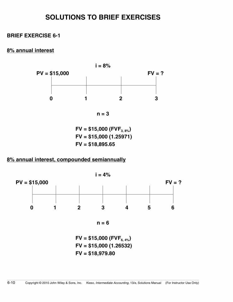
SOLUTIONS TO BRIEF EXERCISES BRIEF EXERCISE 6-1 8% annual interest

i = 8% PV = $15,000 FV = ?

0 1 2 3

n = 3

FV = $15,000 (FVF3, 8%) FV = $15,000 (1.25971) FV = $18,895.65 8% annual interest, compounded semiannually

i = 4% PV = $15,000 FV = ?

0 1 2 3 4 5 6

n = 6

FV = $15,000 (FVF6, 4%) FV = $15,000 (1.26532) FV = $18,979.80


BRIEF EXERCISE 6-2

12% annual interest

i = 12%

PV = ? FV = $25,000

0 1 2 3 4

n = 4

PV = $25,000 (PVF4, 12%)

PV = $25,000 (.63552)

PV = $15,888

12% annual interest, compounded quarterly

i = 3%

PV = ? FV = $25,000

0 1 2 14 15 16

n = 16

PV = $25,000 (PVF16, 3%)

PV = $25,000 (.62317)

PV = $15,579.25


BRIEF EXERCISE 6-3

i = ? PV = $30,000 FV = $150,000

0 1 2 19 20 21

n = 21

FV = PV (FVF21, i) PV = FV (PVF21, i)OR

$150,000 = $30,000 (FVF21, i) $30,000 = $150,000 (PVF21, i)

FVF21, i = 5.0000 PVF21, i = .20000

i = 8% i = 8%

BRIEF EXERCISE 6-4

i = 5% PV = $10,000 FV = $17,100

0 ?

n = ?

FV = PV (FVFn, 5%) PV = FV (PVFn, 5%)OR

$17,100 = $10,000 (FVFn, 5%) $10,000 = $17,100 (PVFn, 5%)

FVFn, 5% = 1.71000 PVFn, 5% = .58480

n = 11 years n = 11 years


BRIEF EXERCISE 6-5

First payment today (Annuity Due)

i = 12% R = FV – AD =

$8,000 $8,000 $8,000 $8,000 $8,000 ?

0 1 2 18 19 20

n = 20

FV – AD = $8,000 (FVF – OA20, 12%) 1.12 FV – AD = $8,000 (72.05244) 1.12 FV – AD = $645,589.86 First payment at year-end (Ordinary Annuity)

i = 12% FV – OA = ? $8,000 $8,000 $8,000 $8,000 $8,000

0 1 2 18 19 20

n = 20

FV – OA = $8,000 (FVF – OA20, 12%) FV – OA = $8,000 (72.05244) FV – OA = $576,419.52


BRIEF EXERCISE 6-6

i = 11% FV – OA = R = ? ? ? ? $250,000

0 1 2 8 9 10

n = 10

$250,000 = R (FVF – OA10, 11%)

$250,000 = R (16.72201)

$250,000

16.72201 = R

R = $14,950

BRIEF EXERCISE 6-7

12% annual interest

i = 12% PV = ? FV = $300,000

0 1 2 3 4 5

n = 5

PV = $300,000 (PVF5, 12%)

PV = $300,000 (.56743)

PV = $170,229


BRIEF EXERCISE 6-8 With quarterly compounding, there will be 20 quarterly compounding periods, at 1/4 the interest rate:

PV = $300,000 (PVF20, 3%)

PV = $300,000 (.55368)

PV = $166,104

BRIEF EXERCISE 6-9

i = 10%

FV – OA =

R = $100,000

$16,380 $16,380 $16,380

0 1 2 n

n = ?

$100,000 = $16,380 (FVF – OAn, 10%)

$100,000 FVF – OAn, 10% =

16,380 = 6.10501

Therefore, n = 5 years


BRIEF EXERCISE 6-10

First withdrawal at year-end

i = 8%

PV – OA = R =

? $30,000 $30,000 $30,000 $30,000 $30,000

0 1 2 8 9 10

n = 10

PV – OA = $30,000 (PVF – OA10, 8%)

PV – OA = $30,000 (6.71008)

PV – OA = $201,302

First withdrawal immediately

i = 8%

PV – AD =

?

R =

$30,000 $30,000 $30,000 $30,000 $30,000

0 1 2 8 9 10

n = 10

PV – AD = $30,000 (PVF – AD10, 8%)

PV – AD = $30,000 (7.24689)

PV – AD = $217,407


BRIEF EXERCISE 6-11

i = ?

PV = R =

$793.15 $75 $75 $75 $75 $75

0 1 2 10 11 12

n = 12

$793.15 = $75 (PVF – OA12, i)

$793.15 PVF12, i =

$75 = 10.57533

Therefore, i = 2% per month or 24% per year.

BRIEF EXERCISE 6-12

i = 8%

PV =

$300,000 R = ? ? ? ? ?

0 1 2 18 19 20

n = 20

$300,000 = R (PVF – OA20, 8%)

$300,000 = R (9.81815)

R = $30,556


BRIEF EXERCISE 6-13

i = 12%

R =

$30,000 $30,000 $30,000 $30,000 $30,000

12/31/09 12/31/10 12/31/11 12/31/15 12/31/16 12/31/17

n = 8

FV – OA = $30,000 (FVF – OA8, 12%)

FV – OA = $30,000 (12.29969)

FV – OA = $368,991

BRIEF EXERCISE 6-14

i = 8%

PV – OA = R =

? $25,000 $25,000 $25,000 $25,000

0 1 2 3 4 5 6 11 12

n = 4 n = 8

PV – OA = $25,000 (PVF – OA12–4, 8%) PV – OA = $25,000 (PVF – OA8, 8%)(PVF4, 8%)

OR

PV – OA = $25,000 (7.53608 – 3.31213) PV – OA = $25,000 (5.74664)(.73503)

PV – OA = $105,599 PV – OA = $105,599


BRIEF EXERCISE 6-15

i = 8%

PV = ?

PV – OA = R = $2,000,000

? $140,000 $140,000 $140,000 $140,000 $140,000

0 1 2 8 9 10

n = 10

$2,000,000 (PVF10, 8%) = $2,000,000 (.46319) = $ 926,380

$140,000 (PVF – OA10, 8%) = $140,000 (6.71008) 939,411

$1,865,791

BRIEF EXERCISE 6-16

PV – OA = $20,000

$4,727.53 $4,727.53 $4,727.53 $4,727.53

0 1 2 5 6

$20,000 = $4,727.53 (PV – OA6, i%)

(PV – OA6, i%) = $20,000 ÷ $4,727.53

(PV – OA6, i%) = 4.23054

Therefore, i% = 11


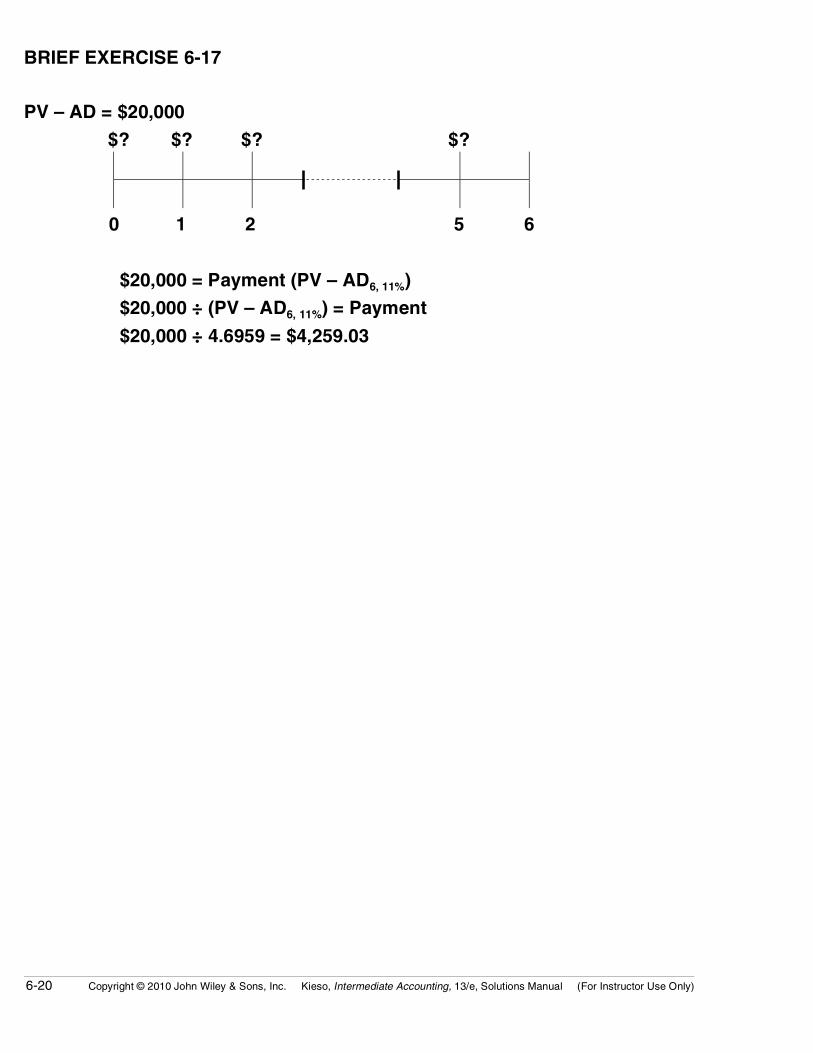
BRIEF EXERCISE 6-17

PV – AD = $20,000

$? $? $? $?

0 1 2 5 6

$20,000 = Payment (PV – AD6, 11%)

$20,000 ÷ (PV – AD6, 11%) = Payment

$20,000 ÷ 4.6959 = $4,259.03


SOLUTIONS TO EXERCISES EXERCISE 6-1 (5–10 minutes) (a) (b) Rate of Interest Number of Periods 1. a. 9% 9 b. 2% 20 c. 5% 30 2. a. 9% 25 b. 4% 30 c. 3% 28 EXERCISE 6-2 (5–10 minutes) (a) Simple interest of $2,400 ($30,000 X 8%) per year X 8.... $19,200 Principal ............................................................................... 30,000 Total withdrawn.......................................................... $49,200 (b) Interest compounded annually—Future value of

1 @ 8% for 8 periods .....................................................

1.85093 X $30,000 Total withdrawn.......................................................... $55,527.90 (c) Interest compounded semiannually—Future

value of 1 @ 4% for 16 periods ....................................

1.87298 X $30,000 Total withdrawn.......................................................... $56,189.40 EXERCISE 6-3 (10–15 minutes) (a) $9,000 X 1.46933 = $13,223.97. (b) $9,000 X .43393 = $3,905.37. (c) $9,000 X 31.77248 = $285,952.32. (d) $9,000 X 12.46221 = $112,159.89.


EXERCISE 6-4 (15–20 minutes) (a) Future value of an ordinary

annuity of $5,000 a period for 20 periods at 8%

$228,809.80

($5,000 X 45.76196)

Factor (1 + .08) X 1.08 Future value of an annuity

due of $5,000 a period at 8%

$247,114.58

(b) Present value of an ordinary

annuity of $2,500 for 30 periods at 10%

$23,567.28

($2,500 X 9.42691)

Factor (1 + .10) X 1.10 Present value of annuity

due of $2,500 for 30 periods at 10%

$25,924.00

(Or see Table 6-5 which gives $25,924.03)

(c) Future value of an ordinary annuity of $2,000 a period for 15 periods at 10%

$63,544.96

($2,000 X 31.77248)

Factor (1 + 10) X 1.10 Future value of an annuity

due of $2,000 a period for 15 periods at 10%

$69,899.46

(d) Present value of an ordinary

annuity of $3,000 for 6 periods at 9%

$13,457.76

($3,000 X 4.48592)

Factor (1 + .09) X 1.09 Present value of an annuity

due of $3,000 for 6 periods at 9%

$14,668.96

(Or see Table 6-5)

EXERCISE 6-5 (10–15 minutes) (a) $50,000 X 4.96764 = $248,382. (b) $50,000 X 8.31256 = $415,628. (c) ($50,000 X 3.03735 X .50663) = $76,940.63. or (5.65022 – 4.11141) X $50,000 = $76,940.50 (difference of $.13 due to

rounding).


EXERCISE 6-6 (15–20 minutes)

(a) Future value of $12,000 @ 10% for 10 years ($12,000 X 2.59374) = $31,124.88(b) Future value of an ordinary annuity of $620,000 at 10% for 15 years ($620,000 X 31.77248) $19,698,937.00 Deficiency ($20,000,000 – $19,698,937) $301,063.00 (c) $75,000 discounted at 8% for 10 years: $75,000 X .46319 = $34,739.25 Accept the bonus of $40,000 now. (Also, consider whether the 8% is an appropriate discount rate since

the president can probably earn compound interest at a higher rate without too much additional risk.)


(a) $100,000 X .31524 = $ 31,524.00 + $10,000 X 8.55948 = 85,594.80 $117,118.80

(b) $100,000 X .23939 = $ 23,939.00 + $10,000 X 7.60608 = 76,060.80 $ 99,999.80

The answer should be $100,000; the above computation is off by 20¢ due to rounding.

(c) $100,000 X .18270 = $18,270.00 + $10,000 X 6.81086 = 68,108.60 $86,378.60


EXERCISE 6-8 (10–15 minutes) (a) Present value of an ordinary annuity of 1 for 4 periods @ 8% 3.31213 Annual withdrawal X $25,000 Required fund balance on June 30, 2013 $82,803.25 (b) Fund balance at June 30, 2013 $82,803.25 Future value of an ordinary annuity at 8% 4.50611

= $18,375.77

for 4 years Amount of each of four contributions is $18,375.77 EXERCISE 6-9 (5–10 minutes) The rate of interest is determined by dividing the future value by the present value and then finding the factor in the FVF table with n = 2 that approxi-mates that number: $118,810 = $100,000 (FVF2, i%) $118,810 ÷ $100,000 = (FVF2, i%) 1.1881 = (FVF2, i%)—reading across the n = 2 row reveals that i = 9%. Note: This problem can also be solved using present value tables. EXERCISE 6-10 (10–15 minutes) (a) The number of interest periods is calculated by first dividing the future

value of $1,000,000 by $148,644, which is 6.72748—the value $1.00 would accumulate to at 10% for the unknown number of interest periods. The factor 6.72748 or its approximate is then located in the Future Value of 1 Table by reading down the 10% column to the 20-period line; thus, 20 is the unknown number of years Mark must wait to become a millionaire.

(b) The unknown interest rate is calculated by first dividing the future value

of $1,000,000 by the present investment of $239,392, which is 4.17725— the amount $1.00 would accumulate to in 15 years at an unknown interest rate. The factor or its approximate is then located in the Future Value of 1 Table by reading across the 15-period line to the 10% column; thus, 10% is the interest rate Elvira must earn on her investment to become a millionaire.


EXERCISE 6-11 (10–15 minutes) (a) Total interest = Total payments—Amount owed today

$155,820 (10 X $15,582) – $100,000 = $55,820. (b) Amos should borrow from the bank, since the 8% rate is lower than

the manufacturer’s 9% rate determined below.

PV – OA10, i% = $100,000 ÷ $15,582 = 6.41766—Inspection of the 10 period row reveals a rate

of 9%. EXERCISE 6-12 (10–15 minutes) Building A—PV = $610,000. Building B— Rent X (PV of annuity due of 25 periods at 12%) = PV $70,000 X 8.78432 = PV $614,902.40 = PV Building C— Rent X (PV of ordinary annuity of 25 periods at 12%) = PV $6,000 X 7.84314 = PV $47,058.84 = PV Cash purchase price $650,000.00 PV of rental income – 47,058.84 Net present value $602,941.16

Answer: Lease Building C since the present value of its net cost is the

smallest.


EXERCISE 6-13 (15–20 minutes) Time diagram:

Messier, Inc. PV = ? i = 5% PV – OA = ? Principal $3,000,000 interest

$165,000 $165,000 $165,000 $165,000 $165,000 $165,000

0 1 2 3 28 29 30

n = 30

Formula for the interest payments: PV – OA = R (PVF – OAn, i)

PV – OA = $165,000 (PVF – OA30, 5%)

PV – OA = $165,000 (15.37245)

PV – OA = $2,536,454

Formula for the principal: PV = FV (PVFn, i)

PV = $3,000,000 (PVF30, 5%)

PV = $3,000,000 (0.23138)

PV = $694,140

The selling price of the bonds = $2,536,454 + $694,140 = $3,230,594.



i = 8% R = PV – OA = ? $800,000 $800,000 $800,000

0 1 2 15 16 24 25 n = 15 n = 10 Formula: PV – OA = R (PVF – OAn, i)

PV – OA = $800,000 (PVF – OA25–15, 8%)

PV – OA = $800,000 (10.67478 – 8.55948)

PV – OA = $800,000 (2.11530)

PV – OA = $1,692,240

OR

Time diagram:

i = 8% R = PV – OA = ? $800,000 $800,000 $800,000

0 1 2 15 16 24 25 FV (PVn, i) (PV – OAn, i)


EXERCISE 6-14 (Continued) (i) Present value of the expected annual pension payments at the end of

the 10th year:

PV – OA = R (PVF – OAn, i)

PV – OA = $800,000 (PVF – OA10, 8%)

PV – OA = $800,000 (6.71008)

PV – OA = $5,368,064

(ii) Present value of the expected annual pension payments at the begin-

ning of the current year:

PV = FV (PVFn, i)

PV = $5,368,064 (PVF15,8%)

PV = $5,368,064 (0.31524)

PV = $1,692,228*

*$12 difference due to rounding. The company’s pension obligation (liability) is $1,692,228.


EXERCISE 6-15 (15–20 minutes) (a)

i = 6% PV = $1,000,000 FV = $1,898,000

0 1 2 n = ?

FVF(n, 8%) = $1,898,000 ÷ $1,000,000 = 1.898 reading down the 6% column, 1.898 corresponds to 11 periods.

(b) By setting aside $300,000 now, Lee can gradually build the fund to an

amount to establish the foundation. PV = $300,000 FV = ?

0 1 2 8 9 FV = $300,000 (FVF9, 6%) = $300,000 (1.68948) = $506,844—Thus, the amount needed from the annuity: $1,898,000 – $506,844 = $1,391,156. $? $? $? FV = $1,391,156

0 1 2 8 9 Payments = FV ÷ (FV – OA9, 6%) = $1,391,156 ÷ 11.49132 = $121,061.46.



Amount to be repaid on March 1, 2018.

Time diagram:

i = 6% per six months

PV = $90,000 FV = ?

3/1/08 3/1/09 3/1/10 3/1/16 3/1/17 3/1/18

n = 20 six-month periods

Formula: FV = PV (FVFn, i)

FV = $90,000 (FVF20, 6%)

FV = $90,000 (3.20714)

FV = $288,643

Amount of annual contribution to debt retirement fund.

Time diagram:

i = 10%

R R R R R FV – AD =

R = ? ? ? ? ? $288,643

3/1/13 3/1/14 3/1/15 3/1/16 3/1/17 3/1/18


EXERCISE 6-16 (Continued) 1. Future value of ordinary annuity of 1 for 5 periods at 10% ................................................................................ 6.105102. Factor (1 + .10)..................................................................... X 1.100003. Future value of an annuity due of 1 for 5 periods at 10% ................................................................................ 6.715614. Periodic rent ($288,643 ÷ 6.71561) .................................... $42,981


Time diagram:

i = 11%

R R R

PV – OA = $421,087 ? ? ?

0 1 24 25

n = 25

Formula: PV – OA = R (PVF – OAn, i)

$421,087 = R (PVF – OA25, 11%)

$421,087 = R (8.42174)

R = $421,087 ÷ 8.42174

R = $50,000



i = 8%

PV – OA = ? $400,000 $400,000 $400,000 $400,000 $400,000

0 1 2 13 14 15

n = 15


PV – OA = $400,000 (PVF – OA15, 8%)

PV – OA = $400,000 (8.55948)

R = $3,423,792 The recommended method of payment would be the 15 annual payments of $400,000, since the present value of those payments ($3,423,792) is less than the alternative immediate cash payment of $3,500,000.



i = 8% PV – AD = ?

R =

$400,000 $400,000 $400,000 $400,000 $400,000

0 1 2 13 14 15 n = 15

Formula: Using Table 6-4 Using Table 6-5

PV – AD = R (PVF – OAn, i) PV – AD = R (PVF – ADn, i)

PV – AD = $400,000 (8.55948 X 1.08) PV – AD = $400,000 (PVF – AD15, 8%)

PV – AD = $400,000 (9.24424) PV – AD = $400,000 (9.24424)

PV – AD = $3,697,696 PV – AD = $3,697,696 The recommended method of payment would be the immediate cash pay-ment of $3,500,000, since that amount is less than the present value of the 15 annual payments of $400,000 ($3,697,696).


EXERCISE 6-20 (15–20 minutes) Expected Cash Flow Probability Cash Estimate X Assessment = Flow (a) $ 4,800 20% $ 960 6,300 50% 3,150 7,500 30% 2,250 Total Expected Value $ 6,360 (b) $ 5,400 30% $ 1,620 7,200 50% 3,600 8,400 20% 1,680 Total Expected Value $ 6,900 (c) $(1,000) 10% $ –100 3,000 80% 2,400 5,000 10% 500 Total Expected Value $ 2,800 EXERCISE 6-21 (10–15 minutes) Estimated Cash Probability Expected Outflow X Assessment = Cash Flow $200 10% $ 20 450 30% 135 600 50% 300 750 10% 75 X PV Factor, n = 2, i = 6% Present Value $ 530 X 0.89 $471.70


EXERCISE 6-22 (15–20 minutes) (a) This exercise determines the present value of an ordinary annuity or

expected cash flows as an fair value estimate. Cash flow Probability Expected Estimate X Assessment = Cash Flow $ 380,000 20% $ 76,000 630,000 50% 315,000 750,000 30% 225,000 X PV Factor, n = 8, I = 8% Present Value $ 616,000 X 5.74664 $ 3,539,930 The fair value estimate of the trade name exceeds the carrying value;

thus, no impairment is recorded. (b) This fair value is based on unobservable inputs—Killroy’s own data on

the expected future cash flows associated with the trade name. This fair value estimate is considered Level 3.


TIME AND PURPOSE OF PROBLEMS Problem 6-1 (Time 15–20 minutes) Purpose—to present an opportunity for the student to determine how to use the present value tables in various situations. Each of the situations presented emphasizes either a present value of 1 or a present value of an ordinary annuity situation. Two of the situations will be more difficult for the student because a noninterest-bearing note and bonds are involved. Problem 6-2 (Time 15–20 minutes) Purpose—to present an opportunity for the student to determine solutions to four present and future value situations. The student is required to determine the number of years over which certain amounts will accumulate, the rate of interest required to accumulate a given amount, and the unknown amount of periodic payments. The problem develops the student’s ability to set up present and future value equations and solve for unknown quantities. Problem 6-3 (Time 20–30 minutes) Purpose—to present the student with an opportunity to determine the present value of the costs of competing contracts. The student is required to decide which contract to accept. Problem 6-4 (Time 20–30 minutes) Purpose—to present the student with an opportunity to determine the present value of two lottery payout alternatives. The student is required to decide which payout option to choose. Problem 6-5 (Time 20–25 minutes) Purpose—to provide the student with an opportunity to determine which of four insurance options results in the largest present value. The student is required to determine the present value of options which include the immediate receipt of cash, an ordinary annuity, an annuity due, and an annuity of changing amounts. The student must also deal with interest compounded quarterly. This problem is a good summary of the application of present value techniques. Problem 6-6 (Time 25–30 minutes) Purpose—to present an opportunity for the student to determine the present value of a series of deferred annuities. The student must deal with both cash inflows and outflows to arrive at a present value of net cash inflows. A good problem to develop the student’s ability to manipulate the present value table factors to efficiently solve the problem. Problem 6-7 (Time 30–35 minutes) Purpose—to present the student an opportunity to use time value concepts in business situations. Some of the situations are fairly complex and will require the student to think a great deal before answering the question. For example, in one situation a student must discount a note and in another must find the proper interest rate to use in a purchase transaction. Problem 6-8 (Time 20–30 minutes) Purpose—to present the student with an opportunity to determine the present value of an ordinary annuity and annuity due for three different cash payment situations. The student must then decide which cash payment plan should be undertaken.


Time and Purpose of Problems (Continued) Problem 6-9 (Time 30–35 minutes) Purpose—to present the student with the opportunity to work three different problems related to time value concepts: purchase versus lease, determination of fair value of a note, and appropriateness of taking a cash discount. Problem 6-10 (Time 30–35 minutes) Purpose—to present the student with the opportunity to assess whether a company should purchase or lease. The computations for this problem are relatively complicated. Problem 6-11 (Time 25–30 minutes) Purpose—to present the student an opportunity to apply present value to retirement funding problems, including deferred annuities. Problem 6-12 (Time 20–25 minutes) Purpose—to provide the student an opportunity to explore the ethical issues inherent in applying time value of money concepts to retirement plan decisions. Problem 6-13 (Time 20–25 minutes) Purpose—to present the student an opportunity to compute expected cash flows and then apply present value techniques to determine a warranty liability. Problem 6-14 (Time 20–25 minutes) Purpose—to present the student an opportunity to compute expected cash flows and then apply present value techniques to determine the fair value of an asset. Problems 6-15 (Time 20–25 minutes) Purpose—to present the student an opportunity to estimate fair value by computing expected cash flows and then applying present value techniques to value an asset retirement obligation.


SOLUTIONS TO PROBLEMS PROBLEM 6-1

(a) Given no established value for the building, the fair market value of the note would be estimated to value the building.

Time diagram:

i = 9%

PV = ? FV = $240,000

1/1/10 1/1/11 1/1/12 1/1/13

n = 3

Formula: PV = FV (PVFn, i)

PV = $240,000 (PVF3, 9%)

PV = $240,000 (.77218)

PV = $185,323.20

Cash equivalent price of building................................... $185,323.20

Less: Book value ($250,000 – $100,000) ....................... 150,000.00

Gain on disposal of the building................................ $ 35,323.20


PROBLEM 6-1 (Continued) (b) Time diagram:

i = 11% Principal

$300,000

Interest PV – OA = ? $27,000 $27,000 $27,000 $27,000

1/1/10 1/1/11 1/1/12 1/1/2019 1/1/2020 n = 10

Present value of the principal

FV (PVF10, 11%) = $300,000 (.35218)...................... = $105,654.00 Present value of the interest payments R (PVF – OA10, 11%) = $27,000 (5.88923) .............. = 159,009.21 Combined present value (purchase price)................. $264,663.21

(c) Time diagram:

i = 8% PV – OA = ? $4,000 $4,000 $4,000 $4,000 $4,000

0 1 2 8 9 10 n = 10

Formula: PV – OA = R (PVF – OAn,i)

PV – OA = $4,000 (PVF – OA10, 8%) PV – OA = $4,000 (6.71008)

PV – OA = $26,840.32 (cost of machine)


PROBLEM 6-1 (Continued)

(d) Time diagram:

i = 12%

PV – OA = ? $20,000 $5,000 $5,000 $5,000 $5,000 $5,000 $5,000 $5,000 $5,000

0 1 2 3 4 5 6 7 8 n = 8

Formula: PV – OA = R (PVF – OAn,i)

PV – OA = $5,000 (PVF – OA8, 12%)

PV – OA = $5,000 (4.96764)

PV – OA = $24,838.20

Cost of tractor = $20,000 + $24,838.20 = $44,838.20

(e) Time diagram:

i = 11% PV – OA = ? $120,000 $120,000 $120,000 $120,000

0 1 2 8 9 n = 9


PV – OA = $120,000 (PVF – OA9, 11%)

PV – OA = $120,000 (5.53705)

PV – OA = $664,446


PROBLEM 6-2

(a) Time diagram: i = 8% FV – OA = $90,000 R R R R R R R R R = ? ? ? ? ? ? ? ?

0 1 2 3 4 5 6 7 8 n = 8

Formula: FV – OA = R (FVF – OAn,i)

$90,000 = R (FVF – OA8, 8%)

$90,000 = R (10.63663)

R = $90,000 ÷ 10.63663

R = $8,461.33

(b) Time diagram:

i = 12% FV – AD =

R R R R 500,000 R = ? ? ? ?

40 41 42 64 65 n = 25


PROBLEM 6-2 (Continued) 1. Future value of an ordinary annuity of 1 for

25 periods at 12% ............................................... 133.33387

2. Factor (1 + .12) ....................................................... 1.1200

3. Future value of an annuity due of 1 for 25

periods at 12% .................................................... 149.33393

4. Periodic rent ($500,000 ÷ 149.33393) ................... $3,348.20

(c) Time diagram:

i = 9% PV = $20,000 FV = $47,347

0 1 2 3 n Future value approach Present value approach FV = PV (FVFn, i) PV = FV (PVFn, i) or $47,347 = $20,000 (FVFn, 9%) $20,000 = $47,347 (PVFn, 9%) = $47,347 ÷ $20,000 = $20,000 ÷ $47,347

FVFn, 9% = 2.36735

PVFn, 9% = .42241

2.36735 is approximately the

value of $1 invested at 9% for 10 years.

.42241 is approximately the present value of $1 discounted at 9% for 10 years.



(d) Time diagram:

i = ?

PV = FV =

$19,553 $27,600

0 1 2 3 4

n = 4

Future value approach Present value approach

FV = PV (FVFn, i) PV = FV (PVFn, i)

or

$27,600 = $19,553 (FVF4, i) $19,553 = $27,600 (PVF4, i)

= $27,600 ÷ $19,553 = $19,553 ÷ $27,600

FVF4, i = 1.41155

PVF4, i = .70844

1.41155 is the value of $1

invested at 9% for 4 years.

.70844 is the present value of $1

discounted at 9% for 4 years.


PROBLEM 6-3

Time diagram (Bid A):

i = 9%$69,000

PV – OA = R =

? 3,000 3,000 3,000 3,000 69,000 3,000 3,000 3,000 3,000 0

0 1 2 3 4 5 6 7 8 9 10

n = 9

Present value of initial cost

12,000 X $5.75 = $69,000 (incurred today) ....................... $ 69,000.00

Present value of maintenance cost (years 1–4)

12,000 X $.25 = $3,000

R (PVF – OA4, 9%) = $3,000 (3.23972) ................................... 9,719.16

Present value of resurfacing

FV (PVF5, 9%) = $69,000 (.64993)............................................ 44,845.17

Present value of maintenance cost (years 6–9)

R (PVF – OA9–5, 9%) = $3,000 (5.99525 – 3.88965)............. 6,316.80

Present value of outflows for Bid A ...................................... $129,881.13


PROBLEM 6-3 (Continued) Time diagram (Bid B):

i = 9%

$126,000

PV – OA = R =

? 1,080 1,080 1,080 1,080 1,080 1,080 1,080 1,080 1,080 0

0 1 2 3 4 5 6 7 8 9 10

n = 9

Present value of initial cost

12,000 X $10.50 = $126,000 (incurred today) .......... $126,000.00

Present value of maintenance cost

12,000 X $.09 = $1,080

R (PV – OA9, 9%) = $1,080 (5.99525) ........................... 6,474.87

Present value of outflows for Bid B............................ $132,474.87

Bid A should be accepted since its present value is lower.


PROBLEM 6-4

Lump sum alternative: Present Value = $500,000 X (1 – .46) = $270,000.

Annuity alternative: Payments = $36,000 X (1 – .25) = $27,000.

Present Value = Payments (PV – AD20, 8%)

= $27,000 (10.60360)

= $286,297.20.

Long should choose the annuity payout; its present value is $16,297.20

greater.


PROBLEM 6-5

(a) The present value of $55,000 cash paid today is $55,000. (b) Time diagram:

i = 21/2% per quarter PV – OA = R =

? $4,000 $4,000 $4,000 $4,000 $4,000

0 1 2 18 19 20 n = 20 quarters


PV – OA = $4,000 (PVF – OA20, 21/2%) PV – OA = $4,000 (15.58916)

PV – OA = $62,356.64 (c) Time diagram:

i = 21/2% per quarter $18,000

PV – AD =

R = $1,800 $1,800 $1,800 $1,800 $1,800

0 1 2 38 39 40 n = 40 quarters

Formula: PV – AD = R (PVF – ADn, i)

PV – AD = $1,800 (PVF – AD40, 21/2%) PV – AD = $1,800 (25.73034)

PV – AD = $46,314.61 The present value of option (c) is $18,000 + $46,314.61, or

$64,314.61.


PROBLEM 6-5 (Continued) (d) Time diagram:

i = 21/2% per quarter

PV – OA = R = ? $1,500 $1,500 $1,500 $1,500 PV – OA = R = ? $4,000 $4,000 $4,000

0 1 11 12 13 14 36 37

n = 12 quarters n = 25 quarters

Formulas:

PV – OA = R (PVF – OAn,i) PV – OA = R (PVF – OAn,i)

PV – OA = $4,000 (PVF – OA12, 21/2%) PV – OA = $1,500 (PVF – OA37–12, 21/2%)

PV – OA = $4,000 (10.25776) PV – OA = $1,500 (23.95732 – 10.25776)

PV – OA = $41,031.04 PV – OA = $20,549.34

The present value of option (d) is $41,031.04 + $20,549.34, or

$61,580.38.

Present values:

(a) $55,000.

(b) $62,356.64.

(c) $64,314.61.

(d) $61,580.38.

Option (c) is the best option, based upon present values alone.

PROBLEM 6-6

Tim

e d

iag

ram

:

i =

12%

P

V –

OA

= ?

R =

(

$39,

000)

($3

9,00

0) $

18,0

00

$18

,000

$68

,000

$68

,000

$68

,000

$68

,000

$38

,000

$38

,000

$38

,000

0

1

5

6

1

0 1

1 12

29

30

31

39

40

n

= 5

n

= 5

n

= 2

0 n

= 1

0 (0

– $

30,0

00 –

$9,

000)

($

60,0

00 –

$30

,000

–

$12,

000)

($

110,

000

– $3

0,00

0 –

$12,

000)

($

80,0

00 –

$30

,000

–

$12,

000)

F

orm

ula

s:

PV

– O

A =

R (

PV

F –

OA

n, i)

P

V –

OA

= R

(P

VF

– O

An,

i)

PV

– O

A =

R (

PV

F –

OA

n, i)

P

V –

OA

=R

(PV

F –

OA

n, i)

PV

– O

A =

($39

,000

)(PV

F –

OA

5, 1

2%) P

V –

OA

= $

18,0

00 (P

VF

– O

A10

-5, 1

2%)

PV

– O

A =

$68

,000

(PV

F –

OA

30–1

0, 1

2%)

PV

– O

A =

$38

,000

(PV

F –

OA

40–3

0, 1

2%)

PV

– O

A =

($39

,000

)(3.

6047

8)

PV

– O

A =

$18

,000

(5.6

5022

– 3

.604

78)

PV

– O

A =

$68

,000

(8.0

5518

– 5

.650

22)

PV

– O

A =

$38

,000

(8.2

4378

– 8

.055

18)

PV

– O

A =

($14

0,58

6.42

) P

V –

OA

= $

18,0

00 (2

.045

44)

PV

– O

A =

$68

,000

(2.4

0496

) P

V –

OA

= $

38,0

00 (

.188

60)

PV

– O

A =

$36

,817

.92

PV

– O

A =

$16

3,53

7.28

P

V –

OA

= $

7,16

6.80

P

rese

nt

valu

e o

f fu

ture

net

cas

h in

flo

ws:

$(14

0,58

6.42

) 36

,817

.92

163,

537.

28

7,1

66.8

0 $

66,

935.

58

Sta

cy M

cGill

sh

ou

ld a

ccep

t n

o le

ss t

han

$66

,935

.58

for

her

vin

eyar

d b

usi

nes

s.



PROBLEM 6-7

(a) Time diagram (alternative one):

i = ? PV – OA = $600,000 R = $80,000 $80,000 $80,000 $80,000 $80,000

0 1 2 10 11 12 n = 12

Formulas: PV – OA = R (PVF – OAn, i)

$600,000 = $80,000 (PVF – OA12, i)

PVF – OA12, i = $600,000 ÷ $80,000

PVF – OA12, i = 7.50

7.50 is present value of an annuity of $1 for 12 years discounted at

approximately 8%. Time diagram (alternative two):

i = ? PV = $600,000 FV = $1,900,000

0 1 2 11 12 n = 12



Future value approach Present value approach

FV = PV (FVFn, i) PV = FV (PVFn, i)

or

$1,900,000 = $600,000 (FVF12, i) $600,000 = $1,900,000 (PVF12, i)

FVF12, I = $1,900,000 ÷ $600,000 PVF12, i = $600,000 ÷ $1,900,000

FVF12, I = 3.16667 PVF12, i = .31579

3.16667 is the approximate future

value of $1 invested at 10%

for 12 years.

.31579 is the approximate present

value of $1 discounted at 10%

for 12 years.

Dubois should choose alternative two since it provides a higher rate

of return.

(b) Time diagram:

i = ? ($824,150 – $200,000) PV – OA = R = $624,150 $76,952 $76,952 $76,952 $76,952

0 1 8 9 10

n = 10 six-month periods



Formulas: PV – OA = R (PVF – OAn, i)

$624,150 = $76,952 (PVF – OA10, i)

PV – OA10, i = $624,150 ÷ $76,952

PV – OA10, i = 8.11090

8.11090 is the present value of a 10-period annuity of $1 discounted at

4%. The interest rate is 4% semiannually, or 8% annually.

(c) Time diagram:

i = 5% per six months PV = ? PV – OA = R = ? $32,000 $32,000 $32,000 $32,000 $32,000 ($800,000 X 8% X 6/12)

0 1 2 8 9 10

n = 10 six-month periods [(7 – 2) X 2]

Formulas:

PV – OA = R (PVF – OAn, i) PV = FV (PVFn, i)

PV – OA = $32,000 (PVF – OA10, 5%) PV = $800,000 (PVF10, 5%)

PV – OA = $32,000 (7.72173) PV = $800,000 (.61391)

PV – OA = $247,095.36 PV = $491,128

Combined present value (amount received on sale of note):

$247,095.36 + $491,128 = $738,223.36


PROBLEM 6-7 (Continued) (d) Time diagram (future value of $200,000 deposit)


PV = $200,000 FV = ?

12/31/10 12/31/11 12/31/19 12/31/20

n = 40 quarters

Formula: FV = PV (FVFn, i)

FV = $200,000 (FVF40, 2 1/2%)

FV = $200,000 (2.68506)

FV = $537,012

Amount to which quarterly deposits must grow:

$1,300,000 – $537,012 = $762,988.

Time diagram (future value of quarterly deposits)


R R R R R R R R R R = ? ? ? ? ? ? ? ? ?

12/31/10 12/31/11 12/31/19 12/31/20

n = 40 quarters



Formulas: FV – OA = R (FVF – OAn, i)

$762,988 = R (FVF – OA40, 2 1/2%)

$762,988 = R (67.40255)

R = $762,988 ÷ 67.40255

R = $11,320


PROBLEM 6-8

Vendor A: $18,000 payment X 6.14457 (PV of ordinary annuity 10%, 10 periods) $110,602.26 + 55,000.00 down payment + 10,000.00 maintenance contract $175,602.26 total cost from Vendor A

Vendor B: $9,500 semiannual payment 18.01704 (PV of annuity due 5%, 40 periods) $171,161.88

Vendor C: $1,000 X 3.79079 (PV of ordinary annuity of 5 periods, 10%) $ 3,790.79 PV of first 5 years of maintenance

$2,000 [PV of ordinary annuity 15 per., 10% (7.60608) – X 3.81529 PV of ordinary annuity 5 per., 10% (3.79079)] $ 7,630.58 PV of next 10 years of maintenance

$3,000 [(PV of ordinary annuity 20 per., 10% (8.51356) – X .90748 PV of ordinary annuity 15 per., 10% (7.60608)] $ 2,722.44 PV of last 5 years of maintenance

Total cost of press and maintenance Vendor C: $150,000.00 cash purchase price 3,790.79 maintenance years 1–5 7,630.58 maintenance years 6–15 2,722.44 maintenance years 16–20 $164,143.81 The press should be purchased from Vendor C, since the present value of the cash outflows for this option is the lowest of the three options.


PROBLEM 6-9

(a) Time diagram for the first ten payments:

i = 10%

PV–AD = ? R = $800,000 $800,000 $800,000 $800,000 $800,000 $800,000 $800,000

0 1 2 3 7 8 9 10

n = 10

Formula for the first ten payments:

PV – AD = R (PVF – ADn, i)

PV – AD = $800,000 (PVF – AD10, 10%)

PV – AD = $800,000 (6.75902)

PV – AD = $5,407,216

Formula for the last ten payments:


PV – OA = $400,000 (PVF – OA19 – 9, 10%)

PV – OA = $400,000 (8.36492 – 5.75902)

PV – OA = $400,000 (2.6059)

PV – OA = $1,042,360

Note: The present value of an ordinary annuity is used here, not the

present value of an annuity due.


PROBLEM 6-9 (Continued) The total cost for leasing the facilities is: $5,407,216 + $1,042,360 = $6,449,576.

OR Time diagram for the last ten payments:

i = 10% PV = ? R = $400,000 $400,000 $400,000 $400,000

0 1 2 9 10 17 18 19 FVF (PVFn, i) R (PVF – OAn, i)

Formulas for the last ten payments:

(i) Present value of the last ten payments:


PV – OA = $400,000 (PVF – OA10, 10%)

PV – OA = $400,000 (6.14457)

PV – OA = $2,457,828



(ii) Present value of the last ten payments at the beginning of current

year:

PV = FV (PVFn, i)

PV = $2,457,828 (PVF9, 10%)

PV = $2,457,828 (.42410)

PV = $1,042,365*

*$5 difference due to rounding.

Cost for leasing the facilities $5,407,216 + $1,042,365 = $6,449,581

Since the present value of the cost for leasing the facilities,

$6,449,581, is less than the cost for purchasing the facilities,

$7,200,000, McDowell Enterprises should lease the facilities. (b) Time diagram:

i = 11%

PV – OA = ? R = $15,000 $15,000 $15,000 $15,000 $15,000 $15,000 $15,000

0 1 2 3 6 7 8 9

n = 9




PV – OA = $15,000 (PVF – OA9, 11%)

PV – OA = $15,000 (5.53705)

PV – OA = $83,055.75

The fair value of the note is $83,055.75.

(c) Time diagram:

Amount paid = $792,000

0 10 30 Amount paid = $800,000

Cash discount = $800,000 (1%) = $8,000 Net payment = $800,000 – $8,000 = $792,000 If the company decides not to take the cash discount, then the company can use the $792,000 for an additional 20 days. The implied interest rate for postponing the payment can be calculated as follows: (i) Implied interest for the period from the end of discount period to

the due date:

Cash discount lost if not paid within the discount period Net payment being postponed

= $8,000/$792,000 = 0.010101



(ii) Convert the implied interest rate to annual basis:

Daily interest = 0.010101/20 = 0.00051 Annual interest = 0.000505 X 365 = 18.43%

Since McDowell’s cost of funds, 10%, is less than the implied

interest rate for cash discount, 18.43%, it should continue the policy of taking the cash discount.


PROBLEM 6-10

1. Purchase.

Time diagrams:

Installments

i = 10%

PV – OA = ? R = $350,000 $350,000 $350,000 $350,000 $350,000

0 1 2 3 4 5 n = 5

Property taxes and other costs

i = 10% PV – OA = ? R = $56,000 $56,000 $56,000 $56,000 $56,000 $56,000

0 1 2 9 10 11 12

n = 12



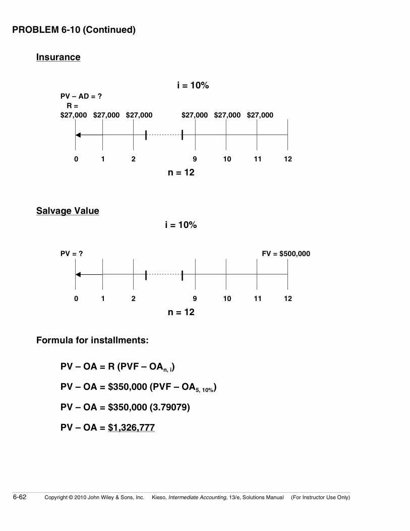
Insurance

i = 10% PV – AD = ? R = $27,000 $27,000 $27,000 $27,000 $27,000 $27,000

0 1 2 9 10 11 12

n = 12

Salvage Value

i = 10%

PV = ? FV = $500,000

0 1 2 9 10 11 12

n = 12

Formula for installments:


PV – OA = $350,000 (PVF – OA5, 10%)

PV – OA = $350,000 (3.79079)

PV – OA = $1,326,777


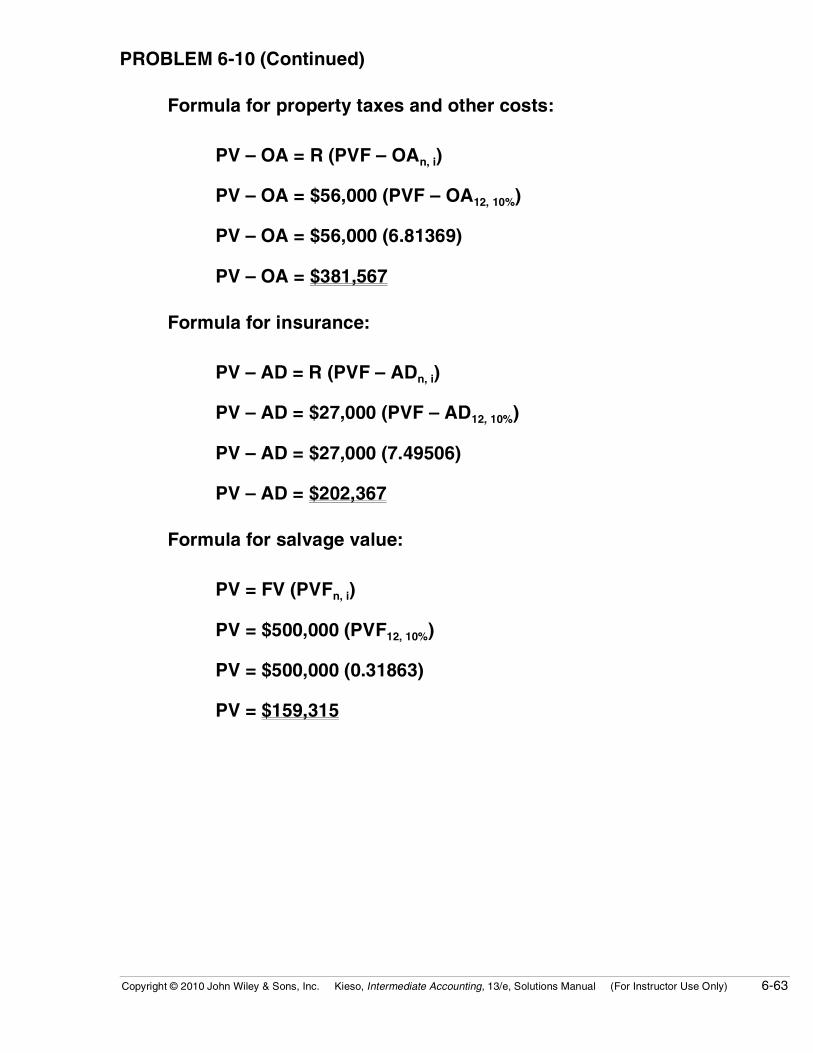
PROBLEM 6-10 (Continued) Formula for property taxes and other costs:


PV – OA = $56,000 (PVF – OA12, 10%)

PV – OA = $56,000 (6.81369)

PV – OA = $381,567

Formula for insurance:


PV – AD = $27,000 (PVF – AD12, 10%)

PV – AD = $27,000 (7.49506)

PV – AD = $202,367

Formula for salvage value:

PV = FV (PVFn, i)

PV = $500,000 (PVF12, 10%)

PV = $500,000 (0.31863)

PV = $159,315



Present value of net purchase costs:

Down payment ......................................................... $ 400,000

Installments .............................................................. 1,326,777

Property taxes and other costs.............................. 381,567

Insurance .................................................................. 202,367

Total costs ................................................................ $2,310,711

Less: Salvage value................................................ 159,315

Net costs................................................................... $2,151,396

2. Lease.

Time diagrams:

Lease payments

i = 10% PV – AD = ? R = $270,000 $270,000 $270,000 $270,000 $270,000

0 1 2 10 11 12

n = 12

Interest lost on the deposit

i = 10% PV – OA = ? R = $10,000 $10,000 $10,000 $10,000 $10,000

0 1 2 10 11 12

n = 12



Formula for lease payments:


PV – AD = $270,000 (PVF – AD12, 10%)

PV – AD = $270,000 (7.49506)

PV – AD = $2,023,666

Formula for interest lost on the deposit:

Interest lost on the deposit per year = $100,000 (10%) = $10,000


PV – OA = $10,000 (PVF – OA12, 10%)

PV – OA = $10,000 (6.81369)

PV – OA = $68,137*

Cost for leasing the facilities = $2,023,666 + $68,137 = $2,091,803

Dunn Inc. should lease the facilities because the present value of the

costs for leasing the facilities, $2,091,803, is less than the present value of the costs for purchasing the facilities, $2,151,396.

*OR: $100,000 – ($100,000 X .31863) = $68,137


PROBLEM 6-11

(a) Annual retirement benefits. Jean–current salary $ 48,000.00 X 2.56330 (future value of 1, 24 periods, 4%) 123,038.40 annual salary during last year of

work X .50 retirement benefit % $ 61,519.00 annual retirement benefit Colin–current salary $ 36,000.00 X 3.11865 (future value of 1, 29 periods, 4%) 112,271.40 annual salary during last year of

work X .40 retirement benefit % $ 44,909.00 annual retirement benefit Anita–current salary $ 18,000.00 X 2.10685 (future value of 1, 19 periods, 4%) 37,923.30 annual salary during last year of

work X .40 retirement benefit % $ 15,169.00 annual retirement benefit Gavin–current salary $ 15,000.00 X 1.73168 (future value of 1, 14 periods, 4%) 25,975.20 annual salary during last year of

work X .40 retirement benefit % $ 10,390.00 annual retirement benefit


PROBLEM 6-11 (Continued) (b) Fund requirements after 15 years of deposits at 12%.

Jean will retire 10 years after deposits stop. $ 61,519.00 annual plan benefit [PV of an annuity due for 30 periods – PV of an X 2.69356 annuity due for 10 periods (9.02181 – 6.32825)] $165,705.00

Colin will retire 15 years after deposits stop.

$44,909.00 annual plan benefit X 1.52839 [PV of an annuity due for 35 periods – PV of an annuity

due for 15 periods (9.15656 – 7.62817)] $68,638.00

Anita will retire 5 years after deposits stop.

$15,169.00 annual plan benefit X 4.74697 [PV of an annuity due for 25 periods – PV of an annuity

due for 5 periods (8.78432 – 4.03735)] $72,007.00

Gavin will retire the beginning of the year after deposits stop.

$10,390.00 annual plan benefit X 8.36578 (PV of an annuity due for 20 periods) $86,920.00



$165,705.00 Jean

68,638.00 Colin

72,007.00 Anita

86,920.00 Gavin

$393,270.00 Required fund balance at the end of the 15 years of

deposits.

(c) Required annual beginning-of-the-year deposits at 12%:

Deposit X (future value of an annuity due for 15 periods at 12%) = FV

Deposit X (37.27972 X 1.12) = $393,270.00

Deposit = $393,270.00 ÷ 41.75329

Deposit = $9,419.


PROBLEM 6-12

(a) The time value of money would suggest that NET Life’s discount rate

was substantially higher than First Security’s. The actuaries at NET Life are making different assumptions about inflation, employee turnover, life expectancy of the work force, future salary and wage levels, return on pension fund assets, etc. NET Life may operate at lower gross and net margins and it may provide fewer services.

(b) As the controller of STL, Brokaw assumes a fiduciary responsibility to

the present and future retirees of the corporation. As a result, he is responsible for ensuring that the pension assets are adequately funded and are adequately protected from most controllable risks. At the same time, Brokaw is responsible for the financial condition of STL. In other words, he is obligated to find ethical ways of increasing the profits of STL, even if it means switching pension funds to a less costly plan. At times, Brokaw’s role to retirees and his role to the corporation can be in conflict, especially if Brokaw is a member of a professional group such as CPAs or CMAs.

(c) If STL switched to NET Life

The primary beneficiaries of Brokaw’s decision would be the corporation and its many stockholders by virtue of reducing 8 million dollars of annual pension costs. The present and future retirees of STL may be negatively affected by Brokaw’s decision because the chance of losing a future benefit may be increased by virtue of higher risks (as reflected in the discount rate and NET Life’s weaker reputation). If STL stayed with First Security In the short run, the primary beneficiaries of Brokaw’s decision would be the employees and retirees of STL given the lower risk pension asset plan. STL and its many stakeholders could be negatively affected by Brokaw’s decision to stay with First Security because of the company’s inability to trim 8 million dollars from its operating expenses.


PROBLEM 6-13

Cash Flow Probability Estimate X Assessment = Expected Cash Flow 2011 $ 2,500 20% $ 500 4,000 60% 2,400 5,000 20% 1,000 X PV Factor, n = 1, I = 5% Present Value $3,900 0.95238 $ 3,714.28 2012 $3,000 30% $ 900 5,000 50% 2,500 6,000 20% 1,200 X PV Factor, n = 2, I = 5% Present Value $4,600 0.90703 $ 4,172.34 2013 $ 4,000 30% $1,200 6,000 40% 2,400 7,000 30% 2,100 X PV Factor, n = 3, I = 5% Present Value $5,700 0.86384 $ 4,923.89 Total Estimated Liability $ 12,810.51


PROBLEM 6-14

Cash Flow Probability Estimate X Assessment = Expected Cash Flow 2011 $ 6,000 40% $ 2,400 9,000 60% 5,400 X PV Factor, n = 1, I = 6% Present Value $ 7,800 0.9434 $7,358.52 2012 $ (500) 20% $ (100) 2,000 60% 1,200 4,000 20% 800 X PV Factor, n = 2, I = 6% Present Value $1,900 0.89 $ 1,691.00 Scrap Value Received at the End of 2012 $ 500 50% $ 250 900 50% 450 X PV Factor, n = 2, I = 6% Present Value $ 700 0.89 $ 623.00 Estimated Fair Value $ 9,672.52


PROBLEM 6-15

(a) The expected cash flows to meet the asset retirement obligation repre-

sent a deferred annuity. Developing a fair value estimate requires determining the present value of the annuity of expected cash flows to be paid in three years and then determine the present value of that amount today.

Cash Flow Probability Estimate X Assessment = Expected Cash Flow $15,000 10% $ 1,500 22,000 30% 6,600 25,000 50% 12,500 30,000 10% 3,000 X PV Factor, n = 3, I = 5% Present Value (deferred 10 yrs) $ 23,600 X 2.72325 $64,269 The value today of the annuity payments to commence in ten years is:

$ 64,269 Present value of annuity X .61391 PV of a lump sum to be paid in 10 periods. $ 39,455

Alternatively, the present value of the deferred annuity can be computed

as follows:

$ 23,600 Expected cash outflows X 1.67184 [PV of an ordinary annuity for 13 periods – PV of an

annuity due for 10 periods (9.39357 – 7.72173)] $ 39,455

(b) This fair value estimate is based on unobservable inputs—Murphy’s

own data on the expected future cash flows associated with the obligation to restore the site. This fair value estimate is considered Level 3.


FINANCIAL REPORTING PROBLEM (a) 1. Long-lived assets, goodwill

For impairment of goodwill and long-lived assets, fair value is deter-

mined using a discounted cash flow analysis. 2. Short-term and long-term debt 3. Postretirement benefit plans 4. Employee stock ownership plans

(b) 1. The following rates are disclosed in the accompanying notes:

Debt

Weighted-Average Effective Interest Rate

At December 31 2007 2006

Short-Term 5.0% 5.3%

Long-Term 3.3% 3.6%


FINANCIAL REPORTING PROBLEM (Continued) Benefit Plans Pension Benefits United States

Other Retiree Benefits

2007 2006 2007 2006 Assumptions used to

determine net periodic benefit cost.

Discount rate 5.2% 4.7% 6.3% 5.2% Expected return on assets 7.2% 7.3% 9.3% 9.2%

Stock-Based Compensation

Assumptions 2007 2006 2005 Weighted average interest rate 4.5% 4.6% 4.4% used in Stock Option Valuation.

2. There are different rates for various reasons:

(1) The maturity dates—short-term vs. long-term. (2) The security or lack of security for debts—mortgages and col-

lateral vs. unsecured loans. (3) Fixed rates and variable rates. (4) Issuances of securities at different dates when differing market

rates were in effect. (5) Different risks involved or assumed. (6) Foreign currency differences—some investments and pay-

ables are denominated in different currencies.


FINANCIAL STATEMENT ANALYSIS CASE

(a) Cash inflows of $375,000 less cash outflows of $125,000 = Net cash

flows of $250,000. $250,000 X 2.48685 (PVF – OA3, 10%) = $621,713 (b) Cash inflows of $275,000 less cash outflows of $155,000 = Net cash

flows of $120,000. $120,000 X 2.48685 (PVF – OA3,10%) = $298,422 (c) The estimate of future cash flows is very useful. It provides an under-

standing of whether the value of gas and oil properties is increasing or decreasing from year to year. Although it is an estimate, it does provide an understanding of the direction of change in value. Also, it can provide useful information to record a write-down of the assets.


PROFESSIONAL RESEARCH: FASB CODIFICATION Search strings: “present value”, present and value, Present value$, “best estimate”, “estimated cash flow”, “expected cash flow”, “fresh-start measurement”, “interest methods of allocation” (a) Statement of Financial Accounting Concepts No. 7, “Using Cash Flow Information and Present

Value in Accounting Measurements (FASB 2000). (b) See Appendix B: APPLICATIONS OF PRESENT VALUE IN FASB STATEMENTS AND APB

OPINIONS, CON7, Par. 119

119. . . . The accompanying table is presented to assist readers in understanding the differences between the conclusions reached in this Statement and those found in FASB Statements and APB Opinions that employ present value techniques in recognition, measurement, or amortization (period-to-period allocation) of assets and liabilities in the statement of financial position.

Some examples are:

∞ Debt payable and related premium or discount ∞ Asset acquired by incurring liabilities in a business combination—“An asset acquired by

incurring liabilities is recorded at cost—that is, at the present value of the amounts to be paid” (paragraph 67(b)).

∞ APB Opinion No. 21, Interest on Receivables and Payables—Note exchanged for property, goods, or services.

∞ Capital lease or operating lease— . . . The lessee’s incremental borrowing rate is used unless (a) the lessor’s implicit rate can be determined and (b) the implicit rate is less than the incremental borrowing rate.

∞ FASB Statement No. 91, Accounting for Nonrefundable Fees and Costs Associated with Originating or Acquiring Loans and Initial Direct Costs of Lease . . . Origination fees and costs are reflected over the life of the loan as an adjustment of the yield on the net investment in the loan.

∞ FASB Statement No. 106, Employers’ Accounting for Postretirement Benefits Other Than Pensions . . . Effective settlement rate—“. . . as opposed to ‘settling’ the obligation, which incorporates the insurer’s risk factor, ‘effectively settling’ the obligation focuses only on the time value of money and ignores the insurer’s cost for assuming the risk of experience losses” (paragraph 188).

∞ FASB Statement No. 121, Accounting for the Impairment of Long-Lived Assets and for Long-Lived Assets to Be Disposed Of . . . The objective is to estimate the fair value of the impaired asset. . . .

(c) 1. CON7, Glossary of terms: Best estimate: The single most-likely amount in a range of possible

estimated amounts; in statistics, the estimated mode. In the past, accounting pronouncements have used the term best estimate in a variety of contexts that range in meaning from “unbiased” to “most likely.” This Statement uses best estimate in the latter meaning, as distinguished from the expected amounts described below.

2. CON7, Glossary of terms: Estimated Cash Flow and Expected Cash Flow: In the past,

accounting pronouncements have used the terms estimated cash flow and expected cash flow interchangeably. In this Statement: Estimated cash flow refers to a single amount to be received or paid in the future. Expected cash flow refers to the sum of probability-weighted amounts in a range of possible estimated amounts; the estimated mean or average.


FASB CODIFICATION (Continued) 3. CON7, Glossary of terms: Fresh-Start Measurements: Measurements in periods following

initial recognition that establishes a new carrying amount unrelated to previous amounts and accounting conventions. Some fresh-start measurements are used every period, as in the reporting of some marketable securities at fair value under FASB Statement No.115, Accounting for Certain Investments in Debt and Equity Securities. In other situations, fresh-start measurements are prompted by an exception or “trigger,” as in a remeasurement of assets under FASB Statement No. 121, Accounting for the Impairment of Long-Lived Assets and for Long-Lived Assets to Be Disposed Of.

4. CON7, Glossary of terms: Interest Methods of Allocation: Reporting conventions that use

present value techniques in the absence of a fresh-start measurement to compute changes in the carrying amount of an asset or liability from one period to the next. Like depreciation and amortization conventions, interest methods are grounded in notions of historical cost. The term interest methods of allocation refers both to the convention for periodic reporting and to the several approaches to dealing with changes in estimated future cash flows.


PROFESSIONAL SIMULATION

Measurementi = 12%

Principal$100,000Interest

PV – OA = ? $10,000 $10,000 $10,000 $10,000 $10,000

0 1 2 3 4 5 n = 5


FV (PVF5, 12%) = $100,000 (.56743) = $56,743.00

Present value of the interest payments

R (PVF – OA5, 12%) = $10,000 (3.60478) = 36,047.80

Combined present value (purchase price) $92,790.80

i = 8%Principal$100,000Interest

PV – OA = ? $10,000 $10,000 $10,000 $10,000 $10,000

0 1 2 3 4 5 n = 5


FV (PVF5, 8%) = $100,000 (.68058) = $ 68,058.00

Present value of the interest payments

R (PVF – OA5, 8%) = $10,000 (3.99271) = 39,927.10

Combined present value (Proceeds) $107,985.10


PROFESSIONAL SIMULATION (Continued) 12%

Inputs:

5

12

?

–10000

–10000

N

I

PV

PMT

FV

Answer: 92,790.45

8%

Inputs:

5

8

?

–10000

–10000

N

I

PV

PMT

FV

Answer: 107,985.42 Valuation

A B C D E F G

1

2 Bond Amortization Schedule

3

4

Date

Cash Interest

Interest

Expense

Bond Discount

Amortization

Carrying

Value of

Bonds

5 Year 0 $92,790.45

6 Year 1 10,000.00 $11,134.85 $1,134.85 93,925.30

7 Year 2 10,000.00 11,271.04 1,271.04 95,196.34

8 Year 3 10,000.00 11,423.56 1.423.56 96,619.90

9 Year 4 10,000.00 11,594.39 1,594.39 98,214.29

10 Year 5 10,000.00 11,785.71 1,785.71 100,000.00

11

12

13

14

15

The following formula is entered in the cells in this column: =+E5*0.12.

The following formula is entered in the cells in this column: =+C6-B6.

The following formula is entered in the cells in this column: =+E5+D6

Documents

ASSIGNMENT CLASSIFICATION TABLE (BY TOPIC)ftp.oz.nthu.edu.tw/~g9771501/isv_sm_ch06.pdf · Accounting Measurements, ... 6-5 CE6-2 (Continued) 50-1 The changes in the carrying amount