Embed Size (px)
Citation preview

ASSIGNMENT #9 Heat Diffusion Using the Explicit Method
DUE - 11/26/17, 11:59pm
You will practice writing a Python program and gain an understanding of the 1-D and 2-D heat
diffusion model, the explicit method for solving finite difference approximations, redirecting
output to a file, and visualization of data. Your program will simulate the diffusion of heat
through a 1-D or 2-D object, such as a wire or plate, using the explicit method to solve for new
time instances.
Background Information:
I. How do we do this? Finite Difference Approximation to Solve Derivatives
II. Function of Space and Time - u(x, t)
Boundary conditions - u(x0, t) = boundary1, u(xn, t) = boundary2
Initial conditions - u(xi, 0) = initial value, i = 1..n-1
III. What exactly do we mean by 1-D heat diffusion on a wire?
leave time continuous
divide on space/finite intervals
IV. Finite Difference Approximation, FDA, for Derivatives
f'’(x) ≈ ( f(x + h) - f(x) ) / h
f'’’(x) ≈ ( f(x + h) - 2 * f(x) + f(x - h) ) / h * h
So what is this h thing?
- the change in the variable you are taking the derivative w/ respect to
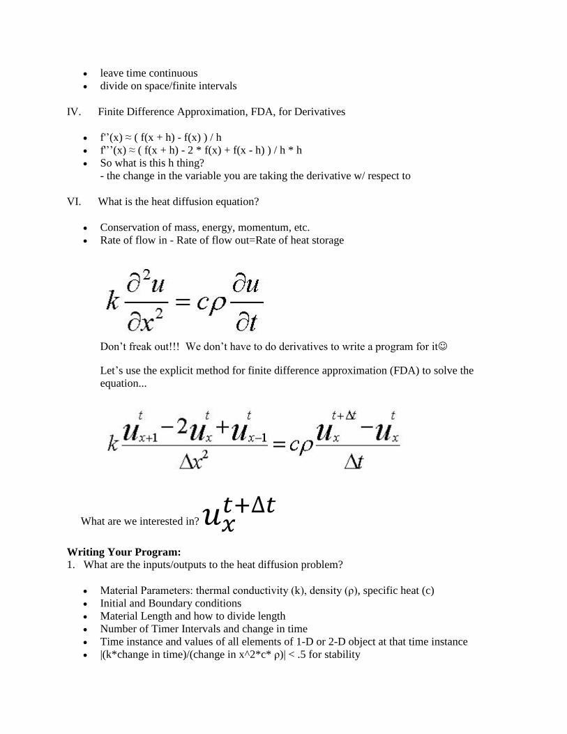
VI. What is the heat diffusion equation?
Conservation of mass, energy, momentum, etc.
Rate of flow in - Rate of flow out=Rate of heat storage
Don’t freak out!!! We don’t have to do derivatives to write a program for it
Let’s use the explicit method for finite difference approximation (FDA) to solve the
equation...
What are we interested in? 𝑢𝑥𝑡+∆𝑡
Writing Your Program:
1. What are the inputs/outputs to the heat diffusion problem?
Material Parameters: thermal conductivity (k), density (ρ), specific heat (c)
Initial and Boundary conditions
Material Length and how to divide length
Number of Timer Intervals and change in time
Time instance and values of all elements of 1-D or 2-D object at that time instance
|(k*change in time)/(change in x^2*c* ρ)| < .5 for stability

2. Pseudocode for Explicit heat diffusion
For all time instances
For all points on material (u)
predict new value at new time instance (equation)
End For
End For
3. Program Input/Output
Read whether the object is 1-D or 2-D from command-line arguments, catch bad input
Read the information from a file, make sure to handle anything that isn’t good (including
an unstable condition for calculation < .5)
Print the time interval and values of the wire at each time instance to the screen
Print the binary information to a file for grads visualization (instructions below)
4. Example Input w/ Thermal Conductivity, Density, and Specific Heat for Nickel (you can
look up other metals here: http://www.engineersedge.com/properties_of_metals.htm).
52.4 0.321 0.12 // Thermal conductivity (k), density (ρ), specific heat (c)
0.0 0.0 100.0 //Initial temp, and boundary conditions (left and right)
10 10 //Length of wire and sections
50 .000335 //Time intervals and change in time
Output:
Since GrADS only visualizes binary data, go back to your python program and add then
information need to print to a binary file:
Import the struct library for packing binary data
import struct
Open the file for writing in binary
f=open(“heat.dat”, ‘wb’)
Write the calculated u for the new time instance
f.write(struct.pack(‘f’, u_new[i]))
Once you have your file, you can use GrADS to visualize your data. Read more about GrADS
Visualization package, http://cola.gmu.edu/grads/gadoc/gadoc.php, and GrADS Gridded Data
Sets, http://cola.gmu.edu/grads/gadoc/aboutgriddeddata.html.
I have this setup in my directory on the ENGR server. Therefore, in order to see things displayed
on the ENGR server, you have to use MobaXterm (Windows) or start Xquartz and ssh with –Y
(MacOS).
Back to the ENGR server…
Download the grads control file, heatdiff.ctl, and the grads script, 1d_grads_script.gs, that will
open the binary data, heat.dat, and display the heat diffusion in grads. You can read the GrADS
descriptor/control files for the data: http://cola.gmu.edu/grads/gadoc/aboutgriddeddata.html#descriptor.
Set the GADDIR environment variable:
setenv GADDIR /nfs/stak/faculty/p/parhammj/grads-2.0.1/lib
Now, you can actually run the grads visualization tool
/nfs/stak/faculty/p/parhammj/grads-2.0.1/bin/grads -l
You should now get a prompt that looks like, ga->, and this is where you can open the
heatdiff.ctl file and then run the 1d_grads_script.gs files to make sure you did everything right.
There is a picture below that shows these commands and the pictures you should get showing the
heat diffusion. You should see heat diffuse down your wire, if your output is correct… quit will
close grads!!!!
Below is the picture you should get:


Now, Extend this to 2-D
t
uc
y
u
x
uk
2
2
2
2
For our 2-D array, we will just make it square to make it easy, i.e. same number of sections in x
and y direction!
Example Input w/ Thermal Conductivity, Density, and Specific Heat for Nickel (you can look up
other metals here: http://www.engineersedge.com/properties_of_metals.htm).
52.4 0.321 0.12 // Thermal conductivity (k), density (ρ), specific heat (c)
0.0 100.0 100.0 //Initial temp, and boundary conditions (left and right)
100.0 100.0 //Boundary conditions (top and bottom)
10 10 //Length of wire and sections
50 .0000335 //Time intervals and change in time
Output:
u i,j
u i,j-1
u i,j+1
u i+1,j
u i-1,j
t
uuc
y
uuu
x
uuuk
t
uc
y
u
x
uk
t
i
tt
ijit
jit
jit
jit
jit
jit
2
1,,1,
2
,1,,1
2
2
2
2
)(
2
)(
2
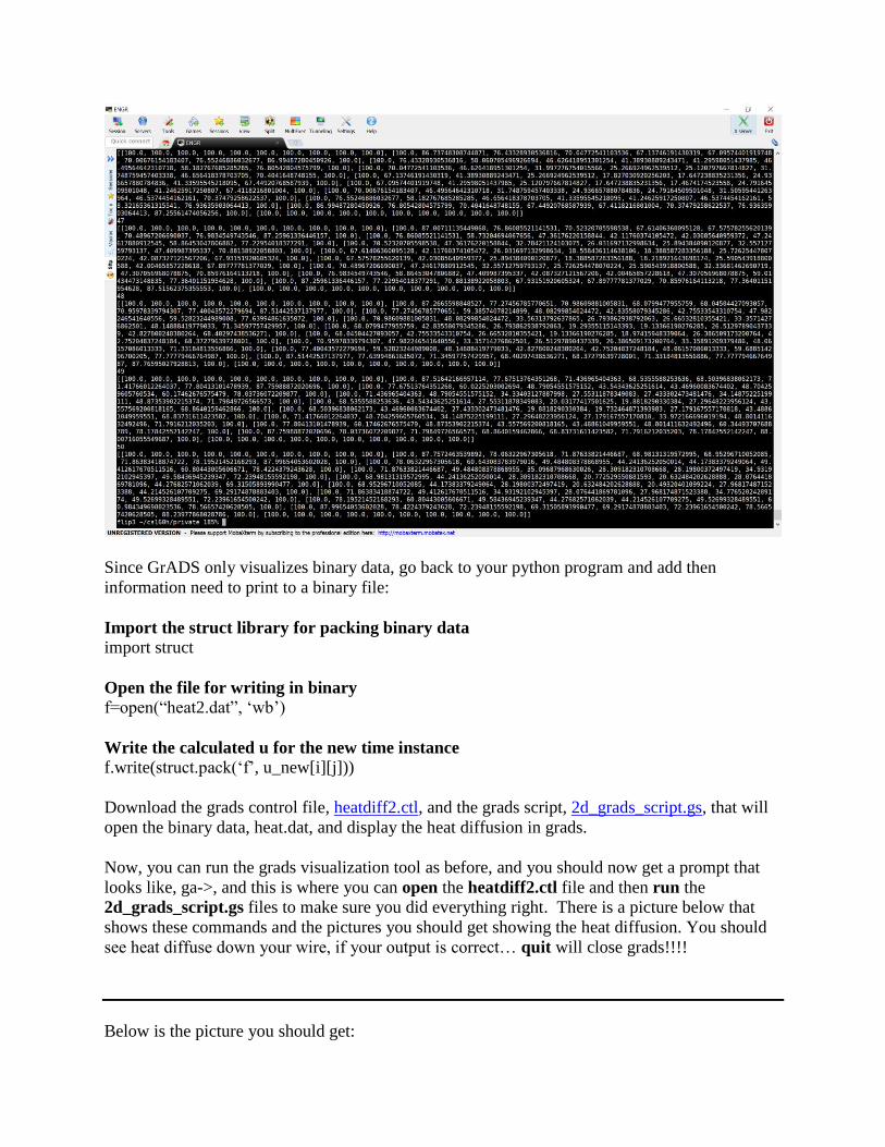
Since GrADS only visualizes binary data, go back to your python program and add then
information need to print to a binary file:
Import the struct library for packing binary data
import struct
Open the file for writing in binary
f=open(“heat2.dat”, ‘wb’)
Write the calculated u for the new time instance
f.write(struct.pack(‘f’, u_new[i][j]))
Download the grads control file, heatdiff2.ctl, and the grads script, 2d_grads_script.gs, that will
open the binary data, heat.dat, and display the heat diffusion in grads.
Now, you can run the grads visualization tool as before, and you should now get a prompt that
looks like, ga->, and this is where you can open the heatdiff2.ctl file and then run the
2d_grads_script.gs files to make sure you did everything right. There is a picture below that
shows these commands and the pictures you should get showing the heat diffusion. You should
see heat diffuse down your wire, if your output is correct… quit will close grads!!!!
Below is the picture you should get: