Assignment 1

Assignment 1 Space Mission Design Optimisation Aman Gupta (SC12B008)

Problem Statement:

A single stage vehicle lifts off from a launch station. The lift off mass is 10000 kg and thrust

at lift off is 150 kN. The vehicle is loaded with 8000 kg of propellant with an Isp of 250 s.

The vehicle rises vertically for 20 seconds then continues its motion a constant turnover of 1

deg/sec for 10 seconds and finally follows gravity turn trajectory till burn out. Analyze and

discuss the trajectory. CD = 0.5. Density at Earth surface = 1.22 kg/m3. Reference area = 2

m2.

Plot the following till burn out:

Time Vs Altitude

Time Vs Velocity

Time Vs. Flight path Angle

Time Vs Dynamic Pressure

Time Vs acceleration

Solution:

The problem is divided in 3 parts. The solution of each part is discussed both numerically and

analytically.

Part 1- The vertical phase. Gaining altitude, but no gain of range. The equations of motion

are written as:

my T D mg (1)

0mx (2)

Where m is the mass of the rocket, T is the Thrust, D is the Drag force and g is the

acceleration due to gravity which is taken as varying as the altitude increases.

Assumptions:

Constant Thrust acting along the vehicle axis.

Propellant weight flow rate is constant.

The mass reduction is only due to propellant outflow.

Result:

Table 1: Results after Vertical take-off phase (time elapsed=10 s)

Property Numerical Result

with no Drag

Numerical Result

with Drag

Analytical Result

Altitude 276.099 m 274.55 m 275.83 m

Velocity 56.74 m/s 56.11 m/s 56.74 m/s

Flight path angle 90 degrees 90 degrees 90 degrees

Dynamic pressure 1890.005 Pa 1848.45 Pa 1890.40 Pa

Acceleration 6.17 m/s2

5.97 m/s2

6.17 m/s2

Part 2-Constant turn over phase. The equations of motion are written as:

sin( ) sin( )my T A mg (3)

cos( ) cos( )mx T A (4)

Figure 1: FBD for a rocket

Where is the angle of attack

is the Gimbal angle

is the flight path angle

A is the Axial force acting opp. to vehicle axis

N is the Normal force perpendicular to vehicle axis

V is the velocity vector

Assumptions:

Centrifugal force is not taken into account i.e. Flat earth model

Thrust acts along vehicle axis.

( ) constant for a small flight time duration.

Table 2: Results after Constant turn over phase (time elapsed=20 s)

Property Numerical result with

no Drag

Numerical Result

with Drag

Analytical Result

Altitude 1167.123 m 1140.684 m 1156.107 m

Velocity 123.74 m/s 118.33 m/s 123.75 m/s

Flight path angle 83.94 degrees 83.89 degrees 83.94 degrees

Dynamic pressure 7943.37 Pa 7291.25 Pa 7956.85 Pa


6.74 m/s2

7.55 m/s2

Part 3-Gravity Turn phase. The equations of motion are written as

sin( )mV T D mg (5)

cos( )mV mg (6)

Take 90 , the above equations can be transformed as:

cos( )mV T D mg (7)

sin( )mV mg (8)

After the second phase is over, Flight path angle is 83.94 degrees which is taken as the initial

angle for gravity turn phase. Drag has to be taken into account for both analytical and

numerical solution.

Assumptions:

Normal and Centrifugal forces are ignored.

Thrust is in vehicle direction.

Axial force A D .

In analytical solution, ( )T D

kW

is taken as constant for small time duration.

Table 3: Results after Gravity turn phase (time elapsed=burn time=130.8 s)

Property Numerical result ( Drag included

after constant turn phase)

Analytical Result

Altitude 64.31 km 64.32 km

Velocity 2607.47 m/s 2609.34 m/s

Flight path angle 30.76 degrees 30.73 degrees

Dynamic pressure 548.47 Pa 553.32 Pa


68.80 m/s2

Graphs:

Figure 2: Trajectory of the Rocket

Figure 3: Altitude vs. Time

Figure 4: Velocity vs. Time

Figure 5: Flight path angle vs. Time

Figure 6: Dynamic Pressure vs. Time

Figure 7: Acceleration vs. Time

Note: In all graphs, analytical and numerical solution with no drag means that drag is not

taken into account till time t=20 sec i.e. till constant turn over phase. After time t=20 sec,

drag is incorporated in both analytical and numerical solution.

Observations:

1. The trajectory is plotted in Figure 1. The rocket is slowly attaining a horizontal

position starting from vertical position initially.

2. Analytical solution matches very well with the numerical result as can be seen from

the Graphs given before. It appears to superimpose the Numerical solution with no

Drag. The analytical solution was faster in computation compared to the numerical

result.

3. Inclusion of Drag plays a very important role. Although the drag is very small as

compared to Thrust but its effect is built up creating a difference of 2.93 km as seen in

Figure 2. No difference as such comes into picture in final velocity and final

acceleration. The flight path angle varies by an angle of 2.34 degrees. Other variations

can be seen in Tables 1 and 2.

4. A sudden kink in the acceleration is seen in Figure 7 at time t=20 sec for analytical

and Numerical solution with no Drag. This is because of the fact that till time t=20

sec, no drag has been taken into account and the drag part only comes into picture for

Gravity turn phase. This kink is absent when Drag is included for whole time.

5. Gravity is assumed to be changing throughout the phase. It changes from 9.81 at the

earth’s surface to 9.61 at burn out.

6. As the time progresses, the weight of the rocket goes down, thereby decreasing the

drag force acting and thus acceleration increases steeply as time increases.

7. Velocity follows the same pattern as the acceleration.

8. Dynamic pressure initially increases and then attains a maxima of around 25720 Pa at

a time of around 60 sec. Although the velocity is continuously increasing, but effect

of density comes into picture at higher altitudes since exponential model is assumed

which makes the dynamic pressure come down.

Code: Both analytical and numerical codes are given below.

Numerical code:

% Numerical Code

clear all;

clc;

lomass=10000; % Mass of Vehicle at lift off

T=150000; % assumed Constant Thrust

propmass=8000; % Mass of propellant Filled

Isp=250; % Assumed Constant Specific Impulse

cd=0.5; % Drag coefficient

S=2; % Reference Area

tb=(propmass*9.81*Isp/T) % burn out time

radius=6378; % Radius of Earth

w(1)= lomass*9.81; % Weight

y(1)=0; % Vertical Height

x(1)=0; % Horizontal Range

vx=0; % Horizontal velocity

vy=0; % Vertical velocity

v(1)=0;

drag(1)=0;

wdot=T/Isp;

i=1;

t(1)=0;

dt=0.01;

% part 1

while(t(i)<=10)

rho(i)=1.22*exp(-y(i)/(7.2*1000));

g=9.81*(radius/(radius+y(i)/1000))^2;

% drag(i)=0.5*cd*S*rho(i)*v(i)*v(i);

drag(i)=0;

accy(i)=(T-drag(i))*g/w(i)- g;

accx(i)=0;

acc(i)=(accx(i)^2+accy(i)^2)^0.5;

vx(i+1)=vx(i)+accx(i)*dt;

vy(i+1)=vy(i)+accy(i)*dt;

v(i+1)=(vy(i+1)^2+vx(i+1)^2)^0.5;

x(i+1)=x(i)+vx(i+1)*dt;

y(i+1)=y(i)+vy(i+1)*dt;

w(i+1)=w(i)-wdot*dt;

t(i+1)=t(i)+dt;

i=i+1;

end

i=i-1;

gamma(1:i)=pi/2;

fprintf(' The Acceleration (m/s2)%f\t', acc(end));

fprintf('\n');

fprintf(' The Altitude%f (km)\t', y(end)/1000);

fprintf('\n');

fprintf(' The Dynamic pressure%f (Pa)\t', 0.5*rho(end)*v(end)^2);

fprintf('\n');

fprintf(' The Velocity %f(m/s)\t',v(end));

fprintf('\n');

fprintf(' The Time %f (s)\t', t(i));

fprintf('\n');

% part 1 over

% part 2 begins

cons_ang=90; %initial value of alpha+gamma

counter=0;

i

t(i)

while (t(i)<=20)

rho(i)=1.22*exp(-y(i)/(7.2*1000));


% drag(i)=0.5*cd*S*rho(i)*v(i)*v(i);

drag(i)=0;

accy(i)=((T-drag(i))*sind(cons_ang))*g/w(i)- g;

accx(i)=((T-drag(i))*cosd(cons_ang))*g/w(i);


vx(i+1)=vx(i)+accx(i)*dt;

vy(i+1)=vy(i)+accy(i)*dt;

v(i+1)=(vy(i+1)^2+vx(i+1)^2)^0.5;

x(i+1)=x(i)+vx(i+1)*dt;

y(i+1)=y(i)+vy(i+1)*dt;


t(i+1)=t(i)+dt;

if counter==100

t(i);

cons_ang=cons_ang-1;

counter=0;

end

gamma(i)=(asin(vy(i)/v(i)));

i=i+1;

counter=counter+1;

end


gamma(end)*(180/pi)


fprintf('\n');


fprintf('\n');


fprintf('\n');


fprintf('\n');

fprintf(' The Time %f (s)\t', t(end));

fprintf('\n');

% part 2 ends

%

% part 3 starts

gamma(i)=gamma(end);

while(t(i)<=tb)

rho(i)=1.22*exp(-y(i)/(7.2*1000));


drag(i)=0.5*cd*S*rho(i)*v(i)*v(i);

dv_dt(i)=((T-drag(i))*g/w(i))-g*sin(gamma(i));

v(i+1)=v(i)+dt*dv_dt(i);

dgamma_dt(i)=-g*cos(gamma(i))/v(i);

gamma(i+1)=gamma(i)+dgamma_dt(i)*dt;

acc(i)=(dv_dt(i)^2+(v(i)*dgamma_dt(i))^2)^0.5;

vx(i+1)=v(i+1)*cos(gamma(i+1));

vy(i+1)=v(i+1)*sin(gamma(i+1));

vxavg=0.5*(vx(i)+vx(i+1));

vyavg=0.5*(vy(i+1)+vy(i));

y(i+1)=y(i)+dt*vyavg;

x(i+1)=x(i)+dt*vxavg;


t(i+1)=t(i)+dt;

i=i+1;

end

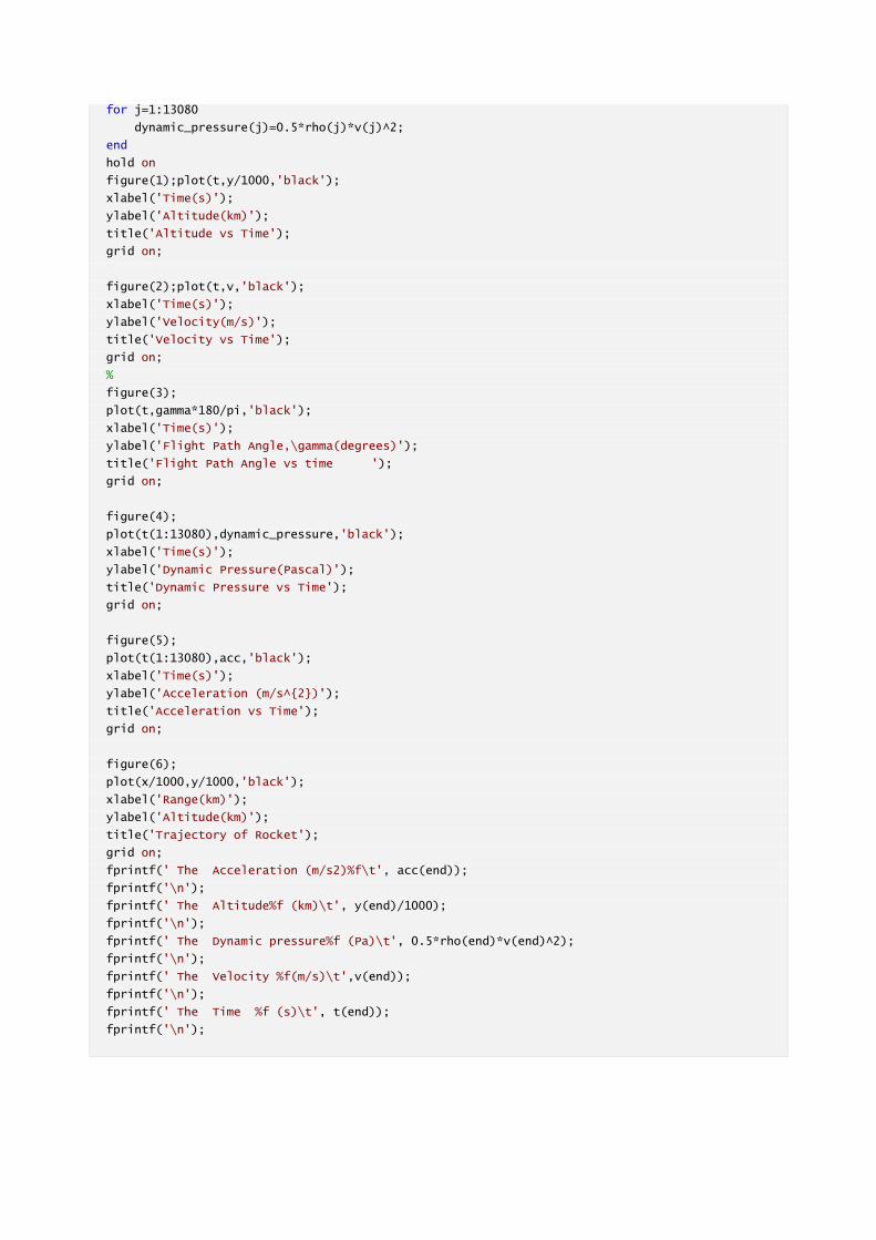
for j=1:13080

dynamic_pressure(j)=0.5*rho(j)*v(j)^2;

end

hold on

figure(1);plot(t,y/1000,'black');

xlabel('Time(s)');

ylabel('Altitude(km)');

title('Altitude vs Time');

grid on;

figure(2);plot(t,v,'black');

xlabel('Time(s)');

ylabel('Velocity(m/s)');

title('Velocity vs Time');

grid on;

%

figure(3);

plot(t,gamma*180/pi,'black');

xlabel('Time(s)');

ylabel('Flight Path Angle,\gamma(degrees)');

title('Flight Path Angle vs time ');

grid on;

figure(4);

plot(t(1:13080),dynamic_pressure,'black');

xlabel('Time(s)');

ylabel('Dynamic Pressure(Pascal)');

title('Dynamic Pressure vs Time');

grid on;

figure(5);

plot(t(1:13080),acc,'black');

xlabel('Time(s)');

ylabel('Acceleration (m/s^{2})');

title('Acceleration vs Time');

grid on;

figure(6);

plot(x/1000,y/1000,'black');

xlabel('Range(km)');


title('Trajectory of Rocket');

grid on;


fprintf('\n');


fprintf('\n');


fprintf('\n');


fprintf('\n');


fprintf('\n');

Analytical Code:

% Analytical Code

clear all;

clc;

lomass=10000; % liftoff mass

T=150000; % Thrust

propmass=8000; % propellant mass

Isp=250; % Specific Impulse

cd=0.5; % Drag coefficient

S=2; % Ref Area

tb=(propmass*9.81*Isp/T) % burn out time

radius=6378; % Radius of Earth in km

w(1)= lomass*9.81; % Liftoff weight

y(1)=0; % Vertical distance

x(1)=0; % Horizontal distance

vx=0; % Horizontal velocity

vy=0; % Vertical velocity

v(1)=0;

drag(1)=0;

wdot=T/Isp;

i=1;

t(1)=0;

dt=0.01;

% part 1

to=0;

while(t(i)<=10)

t(i+1)=to+dt;

rho(i)=1.22*exp(-y(i)/(7.2*1000));


drag(i)=0;

accy(i)=(T-drag(i))*g/w(i)-g;

accx(i)=0;


deltavy=g*Isp*log((w(1)-wdot*to)/(w(1)-wdot*t(i+1)))-g*(t(i+1)-to);

deltavx=0;

vy(i+1)=vy(i)+deltavy;

vx(i+1)=vx(i)+deltavx;

v(i+1)=(vy(i+1)^2+vx(i+1)^2)^0.5;

deltay=g*Isp*(((t(i+1)-w(1)/wdot)*log(w(1)/(w(1)-wdot*t(i+1)))+t(i+1))-((to-

w(1)/wdot)*log(w(1)/(w(1)-wdot*to))+to))-g*(t(i+1)^2-to^2)/2;

deltax=0;

y(i+1)=y(i)+deltay;

x(i+1)=x(i)+deltax;


to=t(i+1);

i=i+1;

end

i=i-1;

gamma(1:i)=pi/2;

phi(1:i)=pi/2-gamma;


fprintf('\n');


fprintf('\n');


fprintf('\n');


fprintf('\n');

fprintf(' The Time %f (s)\t', t(i));

fprintf('\n');

% part 1 over

% part 2 begins

cons_ang=90; %initial value of alpha+gamma

counter=0;

i;

to=t(i);

while (t(i)<=20)

t(i+1)=to+dt;

rho(i)=1.22*exp(-y(i)/(7.2*1000));


drag(i)=0;

accy(i)=((T-drag(i))*sind(cons_ang))*g/w(i)-g;

accx(i)=((T-drag(i))*cosd(cons_ang))*g/w(i);


deltavy=g*Isp*log((w(1)-wdot*to)/(w(1)-wdot*t(i+1)))*sind(cons_ang)-g*(t(i+1)-to);

deltavx=g*Isp*log((w(1)-wdot*to)/(w(1)-wdot*t(i+1)))*cosd(cons_ang);

vy(i+1)=vy(i)+deltavy;

vx(i+1)=vx(i)+deltavx;

v(i+1)=(vy(i+1)^2+vx(i+1)^2)^0.5;

deltay=g*Isp*(((t(i+1)-w(1)/wdot)*log(w(1)/(w(1)-wdot*t(i+1)))+t(i+1))-((to-

w(1)/wdot)*log(w(1)/(w(1)-wdot*to))+to))*sind(cons_ang)-g*(t(i+1)^2-to^2)/2;

deltax=g*Isp*(((t(i+1)-w(1)/wdot)*log(w(1)/(w(1)-wdot*t(i+1)))+t(i+1))-((to-

w(1)/wdot)*log(w(1)/(w(1)-wdot*to))+to))*cosd(cons_ang);

y(i+1)=y(i)+deltay;

x(i+1)=x(i)+deltax;


to=t(i+1);

if counter==100

t(i);


counter=0;

end

gamma(i)=(asin(vy(i)/v(i)));

phi(i)=pi/2-gamma(i);

i=i+1;

counter=counter+1;

end



fprintf('\n');


fprintf('\n');


fprintf('\n');


fprintf('\n');


fprintf('\n');

% part 2 ends

%

% part 3 starts

gamma(i)=gamma(end);

phi(i)=pi/2-gamma(i);

% gamma(i)=89.5*(pi/180);

dphi=(0.01)*(pi/180);

while(t(i)<=tb)

rho(i)=1.22*exp(-y(i)/(7.2*1000));


drag(i)=0.5*cd*S*rho(i)*v(i)*v(i);

dv_dt(i)=((T-drag(i))*g/w(i))-g*cos(phi(i));

dgamma_dt(i)=g*sin(phi(i))/v(i);

acc(i)=(dv_dt(i)^2+(v(i)*dgamma_dt(i))^2)^0.5;

k_ass=(T-drag(i))/w(i); %assumed k for delt time

phi(i+1)=phi(i)+dphi;

gamma(i+1)=(pi/2)-phi(i+1);

so=tan(phi(i)/2);

s1=tan(phi(i+1)/2);

c=v(i)/((so^(k_ass-1))*(1+so^2));

v(i+1)=c*s1^(k_ass-1)*(1+s1^2);

delt=(c/g)*(s1^(k_ass-1)/(k_ass-1)+s1^(k_ass+1)/(k_ass+1))-(c/g)*(so^(k_ass-1)/(k_ass-

1)+so^(k_ass+1)/(k_ass+1));

t(i+1)=t(i)+delt;

vx(i+1)=v(i+1)*sin(phi(i+1));

vy(i+1)=v(i+1)*cos(phi(i+1));

vxavg=0.5*(vx(i)+vx(i+1));

vyavg=0.5*(vy(i+1)+vy(i));

y(i+1)=y(i)+delt*vyavg;

x(i+1)=x(i)+delt*vxavg;

w(i+1)=w(i)-wdot*delt;

i=i+1;

end

for j=1:7321

dynamic_pressure(j)=0.5*rho(j)*v(j)^2;

end

hold on

figure(1);plot(t,y/1000,'black');

xlabel('Time(s)');


title('Altitude vs Time');

grid on;

figure(2);plot(t,v,'black');

xlabel('Time(s)');

ylabel('Velocity(m/s)');

title('Velocity vs Time');

grid on;

figure(3);

plot(t,gamma*180/pi,'black');

xlabel('Time(s)');

ylabel('Flight Path Angle,\gamma(degrees)');

title('Flight Path Angle vs time ');

grid on;

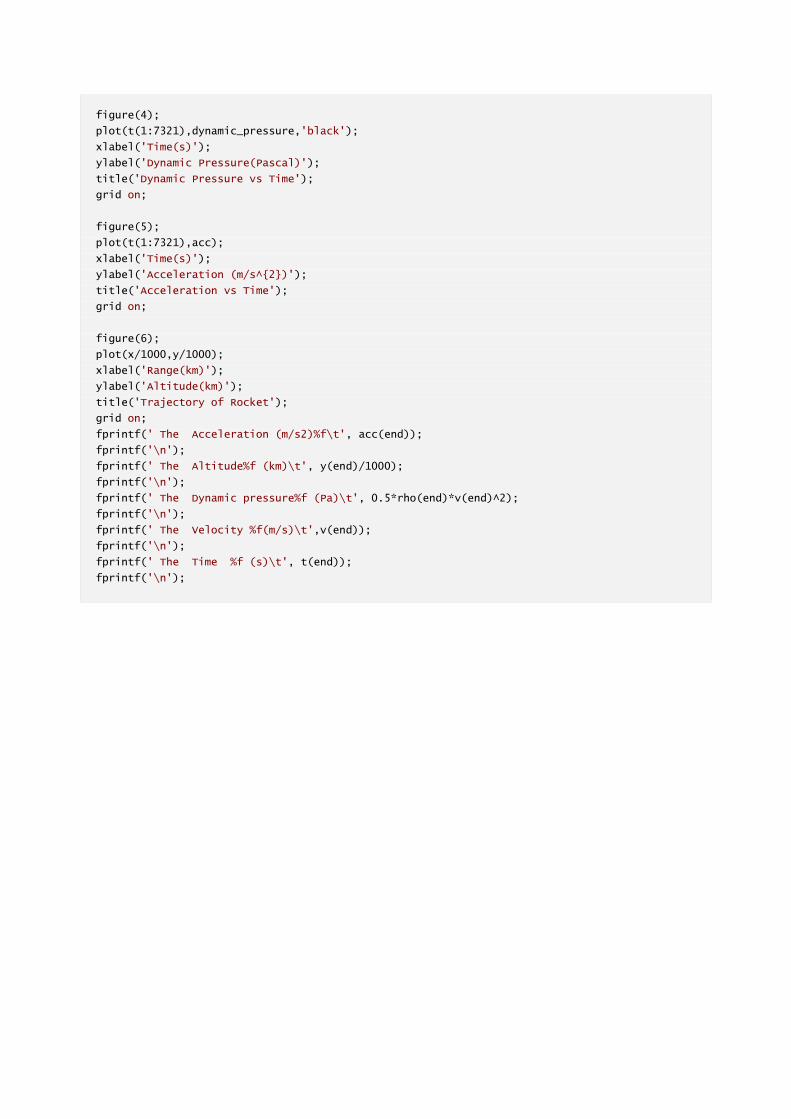
figure(4);

plot(t(1:7321),dynamic_pressure,'black');

xlabel('Time(s)');

ylabel('Dynamic Pressure(Pascal)');

title('Dynamic Pressure vs Time');

grid on;

figure(5);

plot(t(1:7321),acc);

xlabel('Time(s)');

ylabel('Acceleration (m/s^{2})');

title('Acceleration vs Time');

grid on;

figure(6);

plot(x/1000,y/1000);

xlabel('Range(km)');


title('Trajectory of Rocket');

grid on;


fprintf('\n');


fprintf('\n');


fprintf('\n');


fprintf('\n');


fprintf('\n');

Documents

Assignment 1