Asset Pricing when Traders Sell Extreme Winners and Losers

Li An∗†

November 27, 2014

Abstract

This study investigates the asset pricing implications of a newly-documented refinement of

the disposition effect, characterized by investors being more likely to sell a security when the

magnitude of their gains or losses on it increases. I find that stocks with both large unrealized

gains and large unrealized losses, aggregated across investors, outperform others in the following

month (monthly alpha = 0.5-1%, Sharpe ratio = 1.6). This supports the conjecture that these

stocks experience higher selling pressure, leading to lower current prices and higher future re-

turns. This effect cannot be explained by momentum, reversal, volatility, or other known return

predictors, and it also subsumes the previously-documented capital gains overhang effect. More-

over, my findings dispute the view that the disposition effect drives momentum; by isolating the

disposition effect from gains versus that from losses, I find the loss side has a return prediction

opposite to momentum. Overall, this study provides new evidence that investors’ tendencies

can aggregate to affect equilibrium price dynamics; it also challenges the current understanding

of the disposition effect and sheds light on the pattern, source, and pricing implications of this

behavior.

∗PBC School of Finance, Tsinghua University. E-mail: anl@pbcsf.tsinghua.edu.cn†I am deeply indebted to the members of my committee Patrick Bolton, Kent Daniel, Paul Tetlock and Joseph

Stiglitz for many helpful discussions, guidance, and encouragement. I am also grateful for David Hirshleifer, BobHodrick, Gur Huberman, Bernard Salanie, Hao Zhou, Jianfeng Yu and seminar participants at various universitiesand research institutes for helpful comments. All remaining errors are my own. This paper was previously circulatedunder the title “The V-Shaped Disposition Effect”.

1 Introduction

The disposition effect, first described by Shefrin and Statman (1985), refers to the investors’ ten-

dency to sell securities whose prices have increased since purchase rather than those have fallen in

value. This trading behavior is well documented by evidence from both individual investors and

institutions1, across different asset markets2, and around the world3. Several recent studies further

explore the asset pricing implications of this behavioral pattern, and propose it as the source of a few

return anomalies, such as price momentum (e.g., Grinblatt and Han (2005)). In these studies, the

binary pattern of the disposition effect (a difference in selling propensity conditional on gain versus

loss) is commonly presumed as a monotonically increasing relation of investors’ selling propensity

in response to past profits.

However, new evidence calls this view into question. Ben-David and Hirshleifer (2012) examine

individual investor trading data and show that investors’ selling propensity is actually a V-shaped

function of past profits: selling probability increases as the magnitude of gains or losses increases,

with the gain side having a larger slope than the loss side. Figure 1 (Figure 2B in their paper)

illustrates this relation. Notably this asymmetric V-shaped selling schedule remains consistent with

the empirical regularity that investors sell more gains than losses: since the gain side of the V is

steeper than the loss side, the average selling propensity is higher for gains than for losses. This

observed V calls into question the current understanding of how investors sell as a function of

profits. Moreover, it also challenges the studies on equilibrium prices and returns that presume a

monotonically increasing relation between selling propensity and profits.

The current study investigates the pricing implications and consequent return predictability of

this newly-documented refinement of the disposition effect. I refer to the asymmetric V-shaped

selling schedule, which Ben-David and Hirshleifer (2012) suggest to underlie the disposition effect,

as the V-shaped disposition effect. If investors sell more when they have larger gains and losses,

then stocks with BOTH larger unrealized gains and larger unrealized losses (in absolute value) will

experience higher selling pressure. This will temporarily push down current prices and lead to higher

subsequent returns when future prices revert to the fundamental values.

To test this hypothesis, I use stock data from 1970 to 2011 and construct stock-level measures for

1See, for example, Odean (1998) and Grinblatt and Keloharju (2001) for evidence on individual investors, Lockeand Mann(2000), Shapira and Venezia (2001), and Coval and Shumway (2001) for institutional investors.

2See, for example, Genesove and Mayor (2001) in housing market, Heath, Huddart, and Lang (1999) for stockoptions, and Camerer and Weber (1998) in experimental market.

3See Grinblatt and Keloharju (2001), Shapira and Venezia (2001), Feng and Seasholes (2005), among others. Fora thorough survey of the disposition effect, please see the review article by Barber and Odean (2013)

2

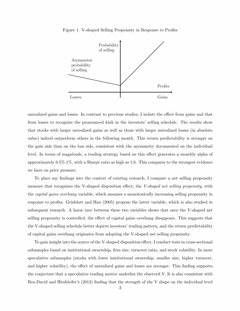
Figure 1. V-shaped Selling Propensity in Response to Profits

Probability of selling

GainsLosses

Asymmetric probability of selling

Profits

unrealized gains and losses. In contrast to previous studies, I isolate the effect from gains and that

from losses to recognize the pronounced kink in the investors’ selling schedule. The results show

that stocks with larger unrealized gains as well as those with larger unrealized losses (in absolute

value) indeed outperform others in the following month. This return predictability is stronger on

the gain side than on the loss side, consistent with the asymmetry documented on the individual

level. In terms of magnitude, a trading strategy based on this effect generates a monthly alpha of

approximately 0.5%-1%, with a Sharpe ratio as high as 1.6. This compares to the strongest evidence

we have on price pressure.

To place my findings into the context of existing research, I compare a net selling propensity

measure that recognizes the V-shaped disposition effect, the V-shaped net selling propensity, with

the capital gains overhang variable, which assumes a monotonically increasing selling propensity in

response to profits. Grinblatt and Han (2005) propose the latter variable, which is also studied in

subsequent research. A horse race between these two variables shows that once the V-shaped net

selling propensity is controlled, the effect of capital gains overhang disappears. This suggests that

the V-shaped selling schedule better depicts investors’ trading pattern, and the return predictability

of capital gains overhang originates from adopting the V-shaped net selling propensity.

To gain insight into the source of the V-shaped disposition effect, I conduct tests in cross-sectional

subsamples based on institutional ownership, firm size, turnover ratio, and stock volatility. In more

speculative subsamples (stocks with lower institutional ownership, smaller size, higher turnover,

and higher volatility), the effect of unrealized gains and losses are stronger. This finding supports

the conjecture that a speculative trading motive underlies the observed V. It is also consistent with

Ben-David and Hirshleifer’s (2012) finding that the strength of the V shape on the individual level

3

is related to investors’ “speculative” characteristics such as trading frequency and gender.

This paper connects to three strands of the literature. First, it contributes to the research on

investors’ trading behaviors, and more specifically how investors trade in light of past profits and

what theories explanation this behavior. While it has become an empirical regularity that investors

sell more gains than losses, most studies focus on the sign of profit (gain or loss) rather than its size,

and the full functional form remains controversial. The V-shaped selling schedule documented by

Ben-David and Hirshleifer (2012) also appears in other studies, such as Barber and Odean (2013)

and Seru, Shumway, and Stoffman (2010), although it is not their focus. On the other side, Odean

(2008) and Grinblatt and Keloharju (2001) show a selling pattern that appears as a monotonically

increasing function of past profits. My findings at the stock level support the V-shaped selling

schedule rather than the monotonic one. A concurrent study by Hartzmark (2013) finds that

investors are more likely to sell extreme winning and extreme losing positions in their portfolio, and

that this behavior can lead to price effects; this is generally consistent with the V-shaped selling

schedule. The shape of the full trading schedule is important because it illuminates the source of this

behavior. Prevalent explanations for the disposition effect, either prospect theory (Kahneman and

Tversky (1979)) or realization utility (Barberis and Xiong (2009, 2012)), attribute this behavioral

tendency to investors’ preference. Although these models can explain the selling pattern partitioned

by the sign of profits by generating a monotonic relation between selling propensity and profits,

reconciling the V-shaped selling schedule in these frameworks is difficult. Instead, belief-based

interpretations may come into play. Cross-sectional subsample results point to a speculative trading

motive (based on investors’ beliefs) as a general cause of this behavior. Moreover, while several

interpretations based on investors’ beliefs are consistent with the V shape on the individual level,

they have different implications for stock-level return predictability. Thus the stock-level evidence in

this paper sheds further light on which mechanisms may hold promise for explaining the V-shaped

disposition effect. Section 5 discusses this point in details.

Second, this study adds to the literature on the disposition effect being relevant to asset pricing.

While investor tendencies and biases are of interest on their own right, they relate to asset pricing

only when individual behaviors aggregate to affect equilibrium price dynamics. Grinblatt and

Han (2005) develop a model in which the disposition effect creates a wedge between price and

fundamental value. Predictable return patterns are generated as the wedge converges in subsequent

periods. Empirically, they construct a stock-level measure of capital gains overhang and show that

it predicts future returns and subsumes the momentum effect. Frazzini (2006) measures capital

4

gains overhang with mutual fund holding data and shows that under-reaction to news caused by

the disposition effect can explain post-earning announcement drift. Goetzmann and Massa (2008)

show that the disposition effect goes beyond predicting stock returns and helps to explain volume

and volatility as well. Shumway and Wu (2007) find evidence in China that the disposition effect

generates momentum-like return patterns. The measures used in these studies are based on the

premise that investors’ selling propensity is a monotonically increasing function of past profits.

This study is the first one to recognize the non-monotonicity when measuring stock-level selling

pressure from unrealized gains and losses and to show that it better captures the predictive return

relation.

Third, this paper contributes to the literature on the extent to which the disposition effect can

explain the momentum effect. Grinblatt and Han (2005) and Weber and Zuchel (2002) develop

models in which the disposition effect generates momentum-like returns, and Grinblatt and Han

(2005) and Shumway and Wu (2007)provide empirical evidence to support this view. In contrast,

Birru (2012) disputes the causality between the disposition effect and momentum. He finds that

following stock splits, which he shows to lack the disposition effect, momentum remains robustly

present. Novy-Marx (2012) shows that a capital gains overhang variable, constructed as in Frazzini

(2006) using mutual fund holding data, does not subsume the momentum effect. My results present

a stronger argument against this view by isolating the disposition effect from gains versus that from

losses: larger unrealized losses predict higher future returns, a direction opposite to what momentum

would predict. Therefore, the disposition effect is unlikely to be a source of momentum.

The rest of the paper is organized as follows. Section 2 describes the analytical framework and

derives hypothesis. Section 3 describes the data and my method for constructing empirical measures.

In section 4, I test the pricing implications of the V-shaped disposition effect using both portfolio

sorts and the Fama-MacBeth regressions. Section 5 discusses the source of the V-shaped disposition

effect and empirically tests it in cross-sectional subsamples. Section 6 discusses the relation between

the disposition effect and momentum. Section 7 runs a battery of robustness checks. Finally, section

8 concludes the paper.

5

2 Analytical Framework and Hypothesis

2.1 Analytical Framework

How do investors’ tendency to trade in light of past profits affects equilibrium prices? I adopt

Grinblatt and Han (2005)’s analytical framework to answer this question. In this framework, the

disposition effect leads to a demand perturbation, which in turn drives stock return predictability.

There exist one single risky stock and two types of investors in this model: type I investors have

rational demand, which only depends on the stock’s fundamental value; type II is disposition-prone

investors, and their demand is a linear function of the stock’s fundamental value and their purchase

price. Moreover, the supply of the stock is assumed to be fixed, normalized to one unit. By

aggregating the demand from all investors, the authors show that the equilibrium price is a linear

combination of the stock’s fundamental value and the disposition-prone investors’ purchase price. I

refer the readers to Grinblatt and Han (2005)’s paper for further details.

For one stock at one time point, investors who do not own the stock are not subject to the

disposition effect, thus they have rational demand for the stock (as potential buyers); for current

stock holders, all or a fraction of them may be prone to the disposition effect and have demand

perturbation. Thus for the purpose of studying the pricing implications, I only need to focus on

the demand function of current stock holders, and I will empirically estimate it in the following

subsection using retail investors’ trading data.

2.2 Revisit of Trading Evidence and Quantitative Derivation of Hypothesis

In this subsection, I revisit the trading evidence documented by Ben-David and Hirshleifer (2012)

and quantitatively derive its pricing implications. I answer two questions here. First, Ben-David

and Hirshleifer (2012) find that both selling and buying schedules have a V-shaped relation with

unrealized profits, thus for the purpose gauging the pricing effect, I estimate the net selling schedule

(selling - buying), which corresponds to investor’s demand. Second, I estimate the relative magni-

tude of demand perturbation on the gain side versus that on the loss side, so that later we can see

if the price effects from the two sides are consistent with this relation.

I start from replicating Ben-David and Hirshleifer (2012)’s results on how paper gains and losses

affect selling and buying. I use the same retail investor trading data (The Odean dataset) and

follow Ben-David and Hirshleifer (2012) for their data screening criteria, variable specifications,

and regression design. I perform a probit regression of a selling (buying) dummy variable on

6

investor’s return since purchase and control variables. Unrealized returns are separated by their

signs (Ret+ = Max{Ret, 0} and Ret− = Min{Ret, 0}), and the controls include an indicator

variable if return is positive, an indicator variable if return is zero, the square root of prior holding

period measured in holding days, the logged purchase price (raw value, not adjusted for stock splits

and distributions), and two stock return volatility variables (calculated using previous 250 trading

days) - one is equal to stock volatility when return is positive, zero otherwise; the other variable is

equal to stock volatility when return is negative, zero otherwise. Regressions are run at different

holding horizons (1 to 20 days, 21 to 250 days, and greater than 250 days), and the observations

are at investor-stock-day level. Please refer to Ben-David and Hirshleifer (2012) for more details.

Table 1 Panel A and Panel B report regression results for selling and buying, respectively.

The estimations are almost the same as Ben-David and Hirshleifer (2012)’s findings4(Table 4 in

their paper): selling and buying probability increase with the magnitude of both paper gains and

losses; for selling schedule, the gain side has a stronger effect, and for buying schedule, the loss

side is stronger; both selling and buying schedule weaken as time since purchase increases, and the

schedules become flat when holding period exceeds 250 trading days.

To map this trading pattern to price effects, I now introduce an alternative definition of return.

Return since purchase in Ben-David and Hirshleifer (2012)’s exercises is defined as the difference

between purchase price and current price normalized by purchase price, i.e., Ret = Pt−P0P0

; on

the other hand, in previous literature on the pricing implications of the disposition effect (e.g.,

Grinblatt and Han (2005) and Frazzini (2006)), stock-level aggregation of investors’ gains and losses

is all defined as a weighted sum of percentage deviation of purchase price from current price, Pt−P0Pt

.

I refer to the latter definition as Ret2 henceforth. Which definition is better?For aggregation at

stock level, Ret2 has a unique advantage in that the weighted sum of all investors’ returns can be

interpreted as the return of a representative investor (∑iωi

Pt−P0iPt

=Pt−

∑iωiP0i

Pt); on the contrary,

definition of Ret does not has this convenience. On selling behavior level, there is no theoretical

guidance on which form of return that investors response to; indeed, the two definitions both mean

to measure the change in value since purchase, with the only difference lying in the normalizing

factor. Therefore I follow the literature on pricing to employ Ret2 to study price effects, and I now

estimate the relation between selling/buying and Ret2 for consistency.

I repeat the regressions in Table 1 Panel A and Panel B, but now replace Ret+ and Ret− with

Ret2+ and Ret2−, where Ret2+ = Max{Pt−P0Pt

, 0} and Ret2− = Min{Pt−P0Pt

, 0}. Table 1 Panel C

4These results are based on a random sample of 10000 accounts, so the numbers can not be exactly identical tothose of Ben-David and Hirshleifer (2012).

7

and Panel D report results for selling and buying, respectively. First of all, comparing with the

corresponding regression results in Panel A and B using the definition of original Ret, coefficients’

t statistics and regression R squares in Panel C and D are of very similar magnitude. This suggests

that Ret2 is no worse than Ret in capturing the relation between trading and unrealized profits.

What’s the shape of investors’ net selling schedule? Comparing columns (1) to (3) in Panel C

with columns (1) to (3) in Panel D, we see that for the same magnitude increase in gains or losses,

selling effect dominates buying effect. To illustrate, consider column (1) in both panels. For prior

holding period less than 20 days, a 1% increase in Ret2+ will raise selling probability by 4.75%,

and will raise the probability of buying additional shares by 1.66%, thus the increase in net selling

probability is 3.09%; on the loss side, a 1% increase in Ret2− will raise selling probability by 2.39%,

and will raise the probability of buying additional shares by 1.86%, thus the increase in net selling

probability is 0.53%. This suggests that investors’ net selling schedule is a V-shaped function, with

the gain side having a steeper slope than the loss side.

What’s the relation between net selling upon a gain and net selling upon a loss? Since trading

schedule becomes flat beyond one year of holding time, I estimate this relation using results in

columns (1) and (2) in Panel C and D. For prior holding period less than 20 days, we have calculated

the net selling schedule and the relative magnitude between gain side and loss side is 3.05%0.53% = 5.75.

For prior holding period between 21 and 250 days (column (2)), on the gain side, a 1% increase in

Ret2+ will lead to a 0.35% − 0.11% = 0.24% increase in net selling probability; on the loss side,

a 1% increase in Ret2− will lead to a 0.09% − 0.05% = 0.04% increase in net selling probability.

Thus the relation between gain side and loss side at this holding horizon is 0.24%0.04% = 6. Weighting

this two ratio by their numbers of observations at corresponding holding periods, a proxy for their

representation in the investor pool, we have the relation between the gain arm and the loss arm of

the V as 5.75× 11442281144228+8106696 + 6× 8106696

1144228+8106696 = 5.95.

Having estimated investors’ demand perturbation, I now link it to the pricing implications and

arrive at the following main hypothesis:

HYPOTHESIS 1. The V-shaped-disposition-prone investors tend to (net) sell more when their

unrealized gains and losses increase in magnitude; this effect is stronger on the gain side, as about

5.9 times the magnitude as that on the loss side. Consequently, on the stock level, stocks with larger

gain overhang and larger (in absolute value) loss overhang will experience higher selling pressure,

5Results in Panel C and D are robust to replacing the dependent variables, selling dummy and buying dummy, bythe number of shares sold and additional shares bought. I report these results in the Appendix Table A2

8

resulting in lower current prices and higher future returns as future prices revert to the fundamental

values. Moreover, the price effects on the gain side and that on the loss side shall be in line with

the relative magnitude.

The rest of the paper will focus on testing the pricing implications, and all remaining empirical

exercises will be conducted on the stock level.

3 Data and Key Variables

3.1 Stock Samples and Filters

I use daily and monthly stock data from CRSP. The sample covers all US common shares (with

CRSP share codes equal to 10 and 11) listed in NYSE, AMEX, and NASDAQ from January 1970

to December 2011. To avoid the impact of the smallest and most illiquid stocks, I eliminate stocks

lower than two dollars in price at the time of portfolio formation, and I require trading activity

during at least 10 days in the past month. I focus on monthly frequency when assessing how gain

and loss overhang affect future returns. My sample results in 1847357 stock-month combinations,

which is approximately 3600 stocks per month on average.

Accounting data and short interest data are from Compustat. Institutional ownership data are

from Thomson-Reuters Institutional Holdings (13F) Database, and this information extends back

to 1980.

3.2 Gains, Losses, and the V-shaped Selling Propensity

For each stock, I measure the aggregate unrealized gains and losses at each month end by using

the volume-weighted percentage deviation of the past purchase price from the current price. The

construction of variables is similar to that in Grinblatt and Han (2005), but with the following

major differences: 1. instead of aggregating all past prices, I measure gains and losses separately;

2. I use daily as opposed to weekly past prices in calculation.

Specifically, I compute the Gain Overhang (Gain) as the following:

9

Gaint =∞∑n=1

ωt−ngaint−n

gaint−n =Pt − Pt−n

Pt· 1{Pt−n≤Pt}

ωt−n =1

kVt−n

n−1∏i=1

[1− Vt−n+i]

(1)

where Vt−n is the turnover ratio at time t − n. The aggregate Gain Overhang is measured as

the weighted average of the percentage deviation of the purchase price from the current price if

the purchase price is lower than the current price. The weight (ωt−n) is a proxy for the fraction of

stocks purchased at day t− n without having been traded afterward.

Symmetrically, the Loss Overhang (Loss) is computed as:

Losst =∞∑n=1

ωt−nlosst−n

losst−n =Pt − Pt−n

Pt· 1{Pt−n>Pt}

ωt−n =1

kVt−n

n−1∏i=1

[1− Vt−n+i]

(2)

It is known that NASDAQ volume data are subject to double counting; therefore I cut the

volume numbers by half for all stocks listed on NASDAQ, to make it roughly comparable to stocks

listed on other exchanges. I do not adjust purchase prices for stock splits and dividends. The reason

is the following: Birru (2012) points out that investors may naively calculate their gains and losses

based on their nominal purchase price, without adjusting for stock splits and dividends. He shows

that the disposition effect is absent after stock splits, and attributes this observation to investor’s

confusion. Later in the robustness check section, I construct gain and loss measures using adjusted

purchase prices; the results remain very similar to those of unadjusted variables. If the current stock

price is above all the historical prices within the past 5 years, Loss is set to be 0, and vice versa for

Gain. Moreover, to be included in the sample, a stock must have at least 60% nonmissing values

within the less of the measuring window and the time it has been appeared in CRSP.

Following Grinblatt and Han (2005), I truncate price history at five years and rescale the weights

for all trading days (with both gains and losses) to sum up to one. In equations (1) and (2), k is the

normalizing constant such that k =∑nVt−n

n−1∏i=1

[1−Vt−n+i]. The choice of a five-year window is due

10

to two reasons. First, Ben-David and Hirshleifer (2012) document the refinement of the disposition

effect among individual traders and they show that the effect becomes flat beyond one year holding

period (Table 4 in their paper, also Table 1 in this paper); however, the disposition effect is far

from restrained to this group of investors (Frazzini (2006), Locke and Mann(2000), Shapira and

Venezia (2001), Coval and Shumway (2001), among others). Taking a five-year window allows the

possibility that other types of investor may have different trading horizons. Second, a five-year

window provides the convenience to compare with the previous literature; note that the sum of

Gain Overhang and Loss Overhang is equal to Capital Gains Overhang (CGO) in Grinblatt and

Han (2005).

That said, I would still like to explore the direct pricing implications of individual investors’

trading horizon. Therefore, based on the one year horizon, I further separate gain and loss overhang

into Recent Gain Overhang (RG), Distant Gain Overhang(DG), Recent Loss Overhang(RL), and

Distant Loss Overhang(DL). The recent overhangs utilize purchase prices within the past one year

of portfolio formation time, while the distant overhangs use purchase prices from the previous one

to five years. As before, the weight on each price is equal to the probability that the stock is last

purchased on that day, and the weights are normalized so that the weights from all four parts sum

up to one.

Putting together the effects of unrealized gains and losses, I name the overall variable as the

V-shaped Net Selling Propensity (V NSP ):

V NSPt = Gaint − 0.17Losst (3)

The coefficient −0.17 indicates the asymmetry in the V shape in investors’ net selling schedule.

According to regression results in section 2.2, the slope on the the gain side of the V is about 5.9

times large as that on the loss side. Thus the coefficient in front of Loss is set to be 15.9 = 0.17.

Panel A in Table 2 presents summary statistics for Recent Gain Overhang, Distant Gain Over-

hang, Recent Loss Overhang, Distant Loss Overhang, Gain Overhang, Loss Overhang, Capital Gains

Overhang and V-shaped Net Selling Propensity. RG, DG, RL, and DL are winsorized at 1% level

in each tail, while Gain, Loss, CGO and V NSP are linear combinations of RG, DG, RL, and DL.

Insert Table 2 about here.

11

3.3 Other Control Variables

To tease out the effect of gain and loss overhang, I control for other variables known to affect fu-

ture returns. By construction, gain and loss overhang utilize prices in the past five years and thus

correlate with past returns; therefore, I control past returns at different horizons. The past twelve-

to-two-month cumulative return Ret−12,−2 is designed to control the momentum effect documented

by Jegadeesh (1990), Jegadeesh and Titman (1993), and De Bondt and Thaler (1985). In Partic-

ular, I separate this return into two variables with one taking on the positive part (Ret+−12,−2 =

Max{Ret−12,−2, 0}) and the other adopting the negative part ( Ret−−12,−2 = Min{Ret−12,−2, 0}).

This approach is taken to address the concern that if the momentum effect is markedly stronger on

the loser side (as documented by Hong, Lim, and Stein (2000)), imposing loser and winner having

the same coefficient in predicting future return will tilt the effects from gains and losses. Specifically,

the loss overhang variable would have to bear part of the momentum loser effect that is not com-

pletely captured by the model specification, as the losers’ coefficient is artificially dragged down by

the winners. Other return controls include the past one-month return Ret−1 for the short-term re-

versal effect, and the past three-to-one-year cumulative return Ret−36,−13 for the long-term reversal

effect.

Since selling propensity variables are constructed as volume-weighted past prices, turnover is

included as a regressor to address the possible effect of volume on predicting return, as shown in

Lee and Swaminathan (2000) and Gervais, Kaniel, and Mingelgrin(2001). The variable turnover

is the average daily turnover ratio in the past year. Idiosyncratic volatility is particularly relevant

here because stocks with large unrealized gains and losses are likely to have high price volatility,

and volatility is well documented (as in Ang, Hodrick, Xing, and Zhang (2006, 2009)) to relate to

low subsequent returns. Thus I control idiosyncratic volatility (ivol), which is constructed as the

volatility of daily return residuals with respect to the Fama-French three-factor model in the past

one year. Book-to-market (logBM) is calculated as in Daniel and Titman (2006), in which this

variable remains the same from July of year t through June of year t + 1 and there is at least a 6

months’ lag between the fiscal year end and the measured return so that there is enough time for

this information to become public. Firm size (logmktcap) is measured as the logarithm of market

capitalization in unit of millions.

Table 2 Panel B summarizes these control variables. All control variables in raw values are

winsorized at 1% level in each tail. Panel C presents correlations of gain and loss variables with

control variables. A somewhat surprising number is the negative correlation of -0.13 between CGO

12

and VNSP, as both variables intend to capture some kind of the disposition effect. I interpret

this negative correlation as follows. The overhang variables are aggregations of Ret2 = Pt−P0Pt

=

Pt−P0P0× P0

Pt. If Pt > P0(gain), then the value of Ret is lessened; if Pt < P0(loss), the value of Ret

is amplified. Therefore, compared with normal definition of return, Ret2 has larger absolute values

on the loss side than on the gain side. Indeed, Gain has a standard deviation of 0.1, while Loss

has a standard deviation of 0.47; CGO has negative mean and median, and is negatively skewed.

While the loss side dominates in value, the gain side has much stronger predictive power for future

returns. Thats why CGO and VNSP are negatively correlated in value (through the loss side), but

their predictive power are to some extent aligned (through the gain side).

4 Empirical Setup and Results

To examine how gain and loss overhang affect future returns, I present two sets of findings. First

I examine returns in sorted portfolios based on the V-shaped net selling propensity. I then employ

Fama and MacBeth (1973) regressions to better control for other known characteristics that may

affect future returns.

4.1 Sorted Portfolios

This subsection investigates return predictability of the V-shaped disposition effect in portfolio sorts.

This illustrates a simple picture of how average returns vary across different levels of the V-shaped

net selling propensity.

Table 3 reports the time series average of mean returns in investment portfolios constructed on

the basis of selling propensity variables.

Insert Table 3 about here.

In Panel A, I sort firms into five quintiles at the end of each month based on their V-shaped net

selling propensity, with quintile 5 representing the portfolio with the largest VNSP. The left side of

the table reports gross-return-weighted portfolio returns6 while the right side shows value-weighted

results. For each weighting method, I show results in portfolio raw returns, DGTW characteristics-

6This follows the weighting practice suggested by Asparouhova, Bessembinder, and Kalcheva (2010) to minimizeconfounding microstructure effects. As they demonstrate, this methodology allows for a consistent estimation of theequal-weighted mean portfolio return. The numbers reported here are almost identical to the equal-weighted results.

13

adjusted returns7, and Carhart four-factor alphas8. All specifications are examined using all months

and using February to December separately9. For comparison, Panel B shows the same set of results

for portfolio returns sorted on capital gains overhang.

In Panel A, portfolio returns increase monotonically with their VNSP quintile. The difference

between quintiles 5 and 1 is generally significant for both gross-return weighted portfolios and

value weighted portfolios. In Panel B, the results confirm Grinblatt and Han’s (2005) finding that

equal-weighted portfolio returns increase with capital gains overhang. However, the value-weighted

portfolios do not have the expected pattern. Moreover, the VNSP effect shows little seasonality,

while the CGO effect is stronger in February to December than in all months. This pattern occurs

because VNSP accounts for the negative impact from the loss side, which can capture the January

reversal caused by tax-loss selling. Overall, these results suggest that, without controlling for other

effects, both VNSP and CGO capture to some extent the price impacts of disposition effect.

A caveat that arises is that VNSP and CGO, both constructed using past prices and volumes,

are correlated with other known return predictors. To better control for confounding factors, in

Panels C and D, I repeat the exercises in Panels A and B, but base the sort on residual selling

propensity variables, instead of the raw values. The residuals are constructed from simultaneous

cross-sectional regressions of the raw selling propensity variables on past returns, size, turnover, and

idiosyncratic volatility. Specifically, the residuals are calculated using the following models:

V NSPt−1 = α+ β1Rett−1 + β2Rett−12,t−2 + β3Rett−36,t−13 + β4logmktcapt−1 + β5turnovert−1 + β6ivolt−1 + εt

CGOt−1 = α+ β1Rett−1 + β2Rett−12,t−2 + β3Rett−36,t−13 + β4logmktcapt−1 + β5turnovert−1 + β6ivolt−1 + εt

Focusing on the gross-return-weighted results in Panel C, the return spread between top and

bottom quintiles based on VNSP (about 0.5% per month) is of similar or larger magnitude than

those in Panel A, and the t-statistics become much larger (around 6, for risk adjusted returns). In

contrast, in Panel D, after controlling for other return predictors, CGO ’s predictive power becomes

very weak; this finding is consistent with regression results in Table 6 Panel B. Note that the value-

7The adjusted return is defined as raw return minus DGTW benchmark return, as developed inDaniel, Grinblatt, Titman, and Wermers (1997) and Wermers (2004). The benchmarks are available viahttp://www.smith.umd.edu/faculty/rwermers/ftpsite/Dgtw/coverpage.htm

8See Fama and French (1993) and Carhart (1997)9Grinblatt and Han (2005) show that their capital gains overhang effect is very different in January and in other

months of the year. They attribute this pattern to return reversal in January that is caused by tax-loss selling inDecember. To rule out the possibility that the results are mainly driven by stocks with large loss overhang (in absolutevalue) having high return in January, I separately report results using February to December only.

14

weighted portfolios in Panels C and D do not have the expected pattern; the return spread between

high and low selling propensity portfolios even becomes negative in some columns. As shown in

section 5 in which I examine results in subsamples, the V-shaped net selling propensity effect is

much stronger among small firms. In fact, the effect from gain side disappears among firms with

size comparable to the top 30% largest firms in NYSE.

4.2 Fama-Macbeth Regression Analysis

This subsection explores the pricing implications of the V-shaped disposition effect in Fama-MacBeth

regressions. While the results using the portfolio approach suggest a positive relation between the

V-shaped net selling propensity and subsequent returns, Fama-MacBeth regressions are more suit-

able for discriminating the unique information in gain and loss variables. I answer three questions

here: 1) Do gain and loss overhang predict future returns, if other known effects are controlled;

2) What is the impact of prior holding period; and 3) Can this V-shaped net selling propensity

subsume previously documented capital gains overhang effect.

4.2.1 The Price Effect of Gains and Losses

I begin by testing Hypothesis 1 (in section 2.2) that the V-shaped net selling schedule on the in-

dividual level can generate price impacts. This means, ceteris paribus, the Gain Overhang will

positively predict future return, while the Loss Overhang will negatively predict future return (be-

cause increased value of Loss Overhang means decreased magnitude of loss); the former should

have a stronger effect compared with the latter. To test this, I consider Fama and MacBeth (1973)

regressions in the following form:

Rett = α+ β1Gaint−1 + β2Losst−1 + γ1X1t−1 + γ2X2t−1 + εt (4)

where Ret is monthly return, Gain and Loss are gain overhang and loss overhang, X1 and

X2 are two sets of control variables, and subscript t denote variables with information up to the

end of month t. X1t−1 is designed to control the momentum effect and it consists of the twelve-

to-two-month return separated by sign, Ret+t−12,t−2 and Ret−t−12,t−2; X2t−1 includes the following

standard characteristics that are also known to affect returns: past one month return Rett−1, past

three-to-one-year cumulative return Rett−36,t−13, log book-to-market ratio logBMt−1, log market

capitalization logmktcapt−1, average daily turnover ratio in the past one year turnovert−1 and

idiosyncratic volatility ivolt−1. Details of these variables’ construction are discussed in section 3.3.

15

I perform the Fama-MacBeth procedure using weighted least square regressions with the weights

equal to the previous one-month gross return to avoid microstructure noise contamination. This

follows the methodology developed by Asparouhova, Bessembinder, and Kalcheva (2010) to correct

the bias from microstructure noise in estimating cross-sectional return premium. The gross-return-

weighted results reported here are almost identical to the equal-weighted results, which suggests

that the liquidity bias is not a severe issue here.

Insert Table 4 about here.

Table 4 presents results from estimating equation (4) and variations of it that omit certain

regressors. For each specification, I report regression estimates for all months in the sample and

for February to December separately. Grinblatt and Han (2005) show strong seasonality in their

capital gains overhang effect and they attribute this pattern to return reversal in January that is

caused by tax-loss selling in December. To address the concern that the estimation is mainly driven

by stocks with large loss overhang (in absolute value) having high return in January, I separately

report results that exclude January from the sample.

Columns (1) and (2) regress future return only on the gain and loss overhang variables; columns

(3) and (4) add the past twelve-to-two month return separated by its sign as regressors; columns (5)

and (6) add controls in X2 to columns (1) and (2); and columns (7) and (8) show the marginal effects

of gain and loss overhang controlling both past return variables and other standard characteristics,

and these two are considered as the most proper specification. Finally, as a basis for comparison,

columns (9) and (10) regress the subsequent one-month return on all control variables only.

Columns (7) and (8) show that with proper control, the estimated coefficient is positive for the

gain overhang and negative for the loss overhang, both as expected. To illustrate, consider the all-

month estimation in column (7). If the gain overhang increases 1%, the future 1-month return will

increase 3.3 basis points, and if the loss overhang increases 1% (the magnitude of loss decreases),

the future 1-month return will decrease around 1.1 basis point. The t-statistics are 8.4 and 10.7

for Gain and Loss, respectively. Since 504 months are used in the estimation, these t-statistics

translate to Sharpe ratios as high as 1.3 and 1.6 for strategies based on the gain overhang and the

loss overhang, respectively. Note that the gain effect is 3 to 4 times as large as the loss effect (in

all months and in February to December), which is roughly in line with the asymmetric V shape in

individual trader’s selling schedule (5.9 times as estimated in section 2.2). A comparison of estimates

for all months and for February to December shows that the coefficients are close, suggesting that

16

the results are not driven by the January effect. From columns (1) and (2) to columns (3) and (4),

from columns (5) and (6) to columns (7) and (8), the change in coefficients shows that controlling

the past twelve-to-two-month return is important to observe the true effect from gains and losses.

Otherwise, stocks with gain (loss) overhang would partly pick up the winner (loser) stocks’ effect,

and the estimate would contain an upward bias because high (low) past return is known to predict

high (low) future return. Moreover, the estimated coefficients on Ret+−12,−2 and Ret−−12,−2 are of

magnitude of difference - Ret−−12,−2 is 5 to 10 times stronger than Ret+−12,−2 in predicting returns;

this suggests that allowing winners and losers to have different coefficients can better capture the

momentum effect10.

The results support Hypothesis 1: stocks with larger gain and loss overhang (in absolute value)

would experience higher selling pressure leading to lower current prices, thus generating higher

future returns when prices revert to the fundamental values. This means that future returns are

higher for stocks with large gains compared with those with small gains, and higher for stocks with

large losses compared to those with small losses. This challenges the current understanding of the

disposition effect that investors’ selling propensity is a monotonically increasing function of past

profits, which would instead predict higher returns for large gains over small gains, but also small

losses over large losses. This evidence also implies that the asymmetric V-shaped selling schedule

of disposition-prone investors is relevant not only on the individual level, but this behavior will also

aggregate to affect equilibrium prices and generate predictable return patterns.

4.2.2 The Impact of Prior Holding Period

I then investigate how the prior holding period affects the return predictability based on the V-

shaped disposition effect. Ben-David and Hirshleifer (2012) show that the V-shaped selling schedule

for individuals is strongest in the short period after purchase. As the holding period becomes longer,

the V becomes flatter, and the loss side eventually becomes flat after 250 trading days since purchase

(Table 4 in their paper, also Table 1 of this paper). Here I decompose Gain and Loss into gains

and losses within one year holding period, and those beyond one year. If we strictly follow the

implications of retail investors’ trading pattern, only the recent gains and losses can generate return

predictability.

10This is consistent with the evidence in Hong, Lim, and Stein (2000), who show that the bulk of the momentumeffect comes from losers, as opposed to winners. However, Israel and Moskowitz (2013) late argue that this phenomenais specific to Hong, Lim, and Stein’s (2000) sample of 1980 to 1996 and is not sustained in a larger sample from 1927to 2011. In my sample from 1970 to 2011, Hong, Lim, and Stein’s (2000) conclusion seems to prevail.

17

To test this implication, I run Fama-MacBeth regressions for the following model:

Rett = α+ β1RGt−1 + β2RLt−1 + β3DGt−1 + β4DLt−1 + γ1X1t−1 + γ2X2t−1 + εt (5)

where Recent Gain Overhang (RG) and Recent Loss Overhang (RL) are overhangs from purchase

prices within the past one year, while Distant Gain Overhang (DG) and Distant Loss Overhang (DL)

are overhangs from purchase prices in the past one to five years. The two sets of control variables

X1 and X2 are the same as in equation (4).

Insert Table 5 about here.

Table 5 illustrates the results separating selling propensity variables from the recent past and

those from the distant past. Again, columns (7) and (8) present estimations from the best model,

and the previous columns omit certain control variables to gauge the relative importance of dif-

ferent effects. In columns (7) and (8), both recent and distant overhang variables exhibit return

predictability, while the recent variables are much stronger than the distant ones. A 1% increase in

recent gains (losses) will lead to a increase of 7.9 basis points (decrease of 1.4 basis points) in monthly

return, while a 1% increase in distant gains (losses) only results in a return increase (decrease) of 2.2

basis points (0.9 basis points). The return predictability of distant gains and losses is not consistent

with the horizon documented by Ben-David and Hirshleifer (2012), which is based on individual

traders; however, the disposition effect is far from restrained to this group of investors (Frazzini

(2006), Locke and Mann(2000), Shapira and Venezia (2001), Coval and Shumway (2001), among

others). Distant gains and losses may capture the effect from other types of investors. Indeed, using

mutual fund holding data, An and Argyle (2014) show that mutual fund managers also exhibit a

V-shaped selling schedule, and this trading pattern lasts beyond one year of holding period. Note

that the relative magnitude between gain and loss effects within one year holding period is at a

multiple of 7.91.4 = 5.6, better aligned with the estimated relation in individual investors’ net selling

schedule; this is consistent with the conjecture that individual investors mainly contribute to price

impact within one year horizon, while the distent gain and loss effects are from other investors.

4.2.3 Comparing V-shaped Net Selling Propensity with Capital Gains Overhang

Finally, I introduce a new variable V-shaped Net Selling Propensity (VNSP) that combines the effects

from the gain side and the loss side. V NSP = Gain−0.17Loss. The coefficient −0.17 resembles an

average relation between the gain side and the loss side on traders’ net selling schedule. I compare

18

the V-shaped net selling propensity variable that recognizes different effects for gains and losses

with the capital gains overhang variable that aggregates all purchase prices, assuming they have

the same impact. Specifically, I test the hypothesis that the previously-documented capital gains

overhang effect, as shown in Grinblatt and Han (2005) and other studies that adopt this measure,

actually originates from this V-shaped disposition effect.

Before I run a horse race between the old and new variables, I first re-run Grinblatt and Han’s

(2005) best model in my sample and show how adding additional control variables affects the results.

Insert Table 6 about here.

Columns (1) and (2) in Table 6 Panel A report Fama-MacBeth regression results from the

following equation (taken from Grinblatt and Han (2005) Table 3 Panel C):

Rett = α+β1CGOt−1+γ1Rett−1+γ2Rett−12,t−2+γ3Rett−36,t−13+γ4logmktcapt−1+γ5turnovert−1+εt

(6)

Focusing on the all-month estimation in column (1), a 1% increase in CGO will lead to a 0.4

basis point increase in the subsequent month return; this effect is weaker compared with Grinblatt

and Han’s (2005) estimation, in which a 1% increase in CGO results in a 0.4 basis point increase

in weekly return. Additionally, controlling capital gains overhang in my sample will not subsume

the momentum effect, rather the momentum effect is actually stronger and more significant than

the capital gains overhang effect. The relation between the disposition effect and momentum will

be discussed in Section 6.

The following four columns show the importance of additional control variables. Columns (3)

and (4) separate the past twelve-to-two-month return by its sign. The losers’ effect is 6 times as large

as that of the winners, with a much larger t-statistic. Allowing winners and losers to have different

levels of effect largely brings down the coefficient for capital gains overhang. Indeed, artificially

equating the coefficients for winners and losers will not fully capture the strong effect on the loser

side; the remaining part of this “low past return predicts low future return” effect will be picked

up by stocks with large unrealized losses (which are likely to have low past returns). This will

artificially associate large unrealized losses with low future returns. Columns (5) and (6) further

control for idiosyncratic volatility; this further dampens the effect of capital gains overhang, which

even becomes negative. This arises because stocks with larger absolute loss overhang are more

likely to be more volatile, which is associated with lower future returns (see Ang, Hodrick, Xing,

19

and Zhang (2006, 2009), among others).

Table 6 Panel B compares the effects of CGO and VNSP, by estimating models that take the

following form:

Rett = α+ β1CGOt−1 + β2V NSPt−1 + γ1X1t−1 + γ2X2t−1 + εt (7)

where the two sets of control variables X1 and X2 are the same as in equation (4) and (5). In

columns (1) (2) (5) and (6), where I don’t control the momentum effect, both variables positively

predict the subsequent one-month return, while VNSP has much larger economic magnitude. Mov-

ing to columns (7) and (8) which include momentum and the whole set of control variables, CGO

has the wrong sign in predicting return, while VNSP remains highly significantly positive. A 1%

increase in VNSP raises the subsequent month return by around 4 basis points; since the average

monthly difference between the 10th and 90th percentile is 23%, return spread between the top and

bottom VNSP portfolio will roughly generate a return of 23% × 0.04% = 0.92% per month. The

t-statistic for the VNSP coefficient is larger than 10; Since 504 months are used in the estimation,

this t-statistic translates into a Sharpe ratio as high as 1.6 (10.38÷√

504×√

12 = 1.6) for a hedged

portfolio based on V-shaped net selling propensity. These results support that V-shaped net selling

propensity dominates capital gains overhang in predicting returns.

5 The Source of the V-shaped Disposition Effect and Cross-sectional

Analysis

This section is devoted to obtaining deeper understanding of the source of the V-shaped disposition

effect. I first discuss several possible mechanisms that may generate the observed V shape on

the individual level; however, the pricing implications of these interpretations diverge. Price-level

evidence shown in the previous section will help to distinguish these potential explanations. I then

examine the effect of gain and loss overhang in different cross-sectional subsamples. This evidence

is consistent with the general conjecture that speculative trading motive leads to the V-shaped

disposition effect.

5.1 The Source of the V-shaped Disposition Effect

An important insight from Ben-David and Hirshleifer (2012) is that investors’ higher propensity to

sell upon gains over losses is not necessarily driven by a preference for realizing gains over losses

20

per se. Indeed, prevalent explanations for the disposition effect, either loss aversion from prospect

theory (Kahneman and Tversky (1979)) or realization utility (Barberis and Xiong (2009, 2012)),

all attribute this behavior to the pain of realizing losses; while these theories can easily generate a

monotonically increasing relation between selling propensity and profits, they are hardly compatible

with the asymmetric V-shaped selling schedule with the minimum at a zero profit point. Instead,

Ben-David and Hirshleifer (2012) suggest belief-based explanations underlie this observed V.

This perspective suggests that changes in beliefs, rather than features of preferences, generate

the V shape. A general conjecture is that investors have a speculative trading motive: they think

they know better than the market does (which may arise from genuine private information or

psychological reasons), thus actively trade in the hope of profits. Investors generally update their

beliefs on a stock after large gains and losses, and this leads to trading activities.

To be more specific, the speculative trading hypothesis encompasses at least three possibilities

that could explain the V shape observed on the individual level. First, the V shape may come from

investors’ limited attention11. Investors may buy a stock and not re-examine their beliefs until the

price fluctuates enough to attract their attention. Thus, large gains and losses are associated with

belief updating and trading activities. The asymmetry may come from investors being more inclined

to re-examine a position when their profits are higher. Second, the V shape may be a consequence of

rational belief-updating. Assume that investors have private information of a stock and have bought

the stock accordingly. As price rises, they may think their information has been incorporated in

the market price thus want to realize the gain; as price declines, they may re-evaluate the validity

of their original beliefs and sell after the loss. A third possibility, irrational belief-updating, conflicts

with the second mechanism. For example, one particular case could be the result of investors’

overconfidence. Think of an extreme case in which investors initially receive private signals that

have no correlation with the true fundamental value; however, they are overconfident about the

signal and think their original beliefs contain genuine information. When price movements lead

to gains and losses, they update their beliefs as in the rational belief-updating case; however, the

trading activities now reflect only noise.

Although all three explanations are consistent with the individual-level V shape, they have

distinct price-level implications. First, the limited attention scenario would predict more selling for

stocks with large gains and losses, but the same mechanism is likely to generate more buying for

these stocks since potential buyers are attracted by the extreme returns12, regardless of whether

11see Barber and Odean (2008), Seasholes and Wu (2007), among others.12Barber and Odean (2008)

21

they currently hold the stock or not. Though we know for current stock holders, the selling effect

seems to dominate, the pricing implication is still ambiguous because buying from non-holders also

comes into play. As to the second interpretation, the rational belief-updating scenario would suggest

trading after gains and losses reflects the process of information being absorbed into price. We would

not see a predictable pattern in future returns in this case. Finally, in the third possibility, irrational

belief-updating, selling is caused by belief changes based on misperceptions and does not draw on

genuine information, thus the downward pressure on current price is temporary and future returns

are predictable. Given the different implications, price-level evidence would help to distinguish the

source of the V-shaped disposition effect: the return predictability shown in section 4 is consistent

with the irrational belief-updating scenario, as opposed to the other two.

5.2 Subsample Analysis: the Impact of Speculativeness

In this subsection, I test the broad conjecture that speculative trading incurs the V-shaped dis-

position effect. This conjecture, encompassing all three possibilities discussed in section 5.1, is in

contrast to preference-based explanations. To assess whether speculative trading can serve as a

possible source, I examine how the effect of gains and losses play out in subsamples based on in-

stitutional ownership, firm size, turnover and volatility. In general, stocks with low institutional

ownership, smaller size, higher turnover, and higher volatility are associated with more speculative

activities, and I test whether the gain and loss overhang effect is stronger among these stocks.

The categorizing variables are defined as follows: institutional ownership is the percentage of

shares outstanding held by institutional investors; firm size refers to a firm’s market capitalization;

turnover, as in section 4, is the average daily turnover ratio within one year; and volatility is

calculated as daily stock return volatility in the past one year. Since institutional ownership,

turnover, and volatility are all largely correlated with firm size, sorting based on the raw variables

may end up testing the role of size in all exercises. To avoid this situation, I base subsamples

on size-adjusted characteristics. Specifically, I first sort all firms into 10 deciles according to their

market capitalization; within each decile, I then equally divide firms into three groups according to

the characteristic of interest (call them low, medium, and high); and finally I collapse across the

size groups. This way, each of the characteristic subsamples contains firms of all size levels. As for

size, the three groups are divided by NYSE break points; the high group contains firms with size in

the largest 30% NYSE firms category, while the low group corresponds to the bottom 30%.

Insert Table 7 about here.

22

In each high and low subsample, I re-examine equation (4) using Fama and Macbeth (1973)

regressions. I only report the results from the best model with all proper controls for all months

and for February to December (corresponding to Table 4 columns (7) and (8)). Table 7 presents

the results.

In the four more speculative subsamples (low institutional ownership, low market capitalization,

high turnover and high volatility), the effects for gains and losses are indeed economically and

statistically stronger than their less speculative counterpart. This finding is consistent with the

investor-level evidence from Ben-David and Hirshleifer (2012), in which the strength of the V shape

in an investor’s selling schedule is found to be associated with his or her “speculative” characteristics

such as trading frequency and gender. As more speculative investors are more likely to be prevalent

in speculative stocks, the stock-level findings suggest that speculation is the source of this individual

behavior.

In the subsample of high market capitalization, the gain effect completely disappears. This

suggests that the V-shaped net selling propensity effect is most prevalent among middle and small

firms. In all other groups, the gain and loss variables exhibit significant predictive power for future

return with the expected sign, and the gain effect is 2 to 6 times as large as the loss effect. This

suggests that the asymmetry between gains and losses is a relatively stable relation.

There are alternative interpretations for the different strength of effect across different stock

groups though. One possibility is that the V-shaped net selling propensity effect is stronger among

stocks for which there is a high limit to arbitrage. Low institutional ownership may reflect less

presence of arbitragers; small firms may be illiquid and relatively hard to arbitrage on; volatility

(especially idiosyncratic volatility) may also represent a limit to arbitrage, as pointed out in Shleifer

and Vishny (1997). However, this interpretation is not consistent with the pattern observed in the

turnover groups - high turnover stocks that attract more arbitragers exhibit stronger gain and loss

effects.

6 The Disposition Effect and Momentum

Recent research highlights the disposition effect as the driver of several return anomalies, among

which price momentum is probably the most prominent one. Grinblatt and Han (2005) suggest

that past returns may be noisy proxies for unrealized gains and losses, and they show that when

the capital gains overhang variable is controlled in their sample, the momentum effect disappears.

23

Shumway and Wu (2007) subsequently use stock trading data from China to test if the disposition

effect drives momentum; though they do not find momentum in their relatively short sample, they

document a momentum-like phenomenon based on unrealized gains and losses and suggest that it

supports the hypothesis. In contrast, Novy-Marx (2012) shows that a capital gains overhang variable

constructed as in Frazzini (2006) using mutual fund holding data does not subsume momentum effect

in the sample from 1980 to 2002: he instead finds that capital gains overhang has no power to predict

returns after the variation in past returns in controlled for. Birru (2012) also disputes the causality

between the disposition effect and momentum; he finds that following stock splits, in which he shows

that the disposition effect is seen to be absent, momentum remains robustly present.

My results lend support to the second camp of research, which claims that the disposition

effect cannot explain momentum. First, with regard to the original capital gains overhang variable

constructed following Grinblatt and Han (2005), results shown in Table 6 Panel A columns (1)

and (2) find this variable does not subsume momentum in my sample of 1970 to 2011. Moreover,

allowing past winners and losers to have different strength of effect (as in columns (3) and (4))

largely reduces the coefficient for capital gains overhang. This suggests that a large portion of

capital gains overhang’s original predictive power comes from picking up momentum effect, when

the functional form of momentum effect is misspecified in the regression.

Second, isolating the disposition effect from gains and from losses presents a stronger argument.

Since the marginal effect from the loss side is negative on future returns, it runs opposite to loser

stocks having lower future returns. Furthermore, Tables 4 shows the importance of controlling the

momentum variable to reveal the true effect from gains and losses.

Last but not least, the asymmetry in the disposition effect and in momentum suggests the at-

tempt to explain momentum using the disposition effect is doomed to failure. Indeed, the disposition

effect mainly originates from the gain side, while momentum is mostly a loser effect. In my sample,

the disposition effect from gains is about 5 times as large as that from losses; for momentum, the

losers have 5 to 10 times the predictive power for future returns compared with the winners. Thus

the disposition effect can hardly generate a return pattern that matches the asymmetry in momen-

tum. There is a caveat though: Israel and Moskowitz (2013) argue that the pronounced asymmetry

in momentum is sample specific; thus the explanatory power of the disposition effect for momentum

might be stronger in other samples.

24

7 Robustness Checks

I now conduct a battery of robustness checks of my results under alternative empirical specifications.

7.1 Alternative specifications and alternative samples

1. Adjusting prices for stock splits and dividends. In the main specification, I aggregate purchase

prices without adjusting for stock splits and dividends. To make sure the results are not driven by

this, I construct alternative overhang variables adjusting for sock splits and dividends and repeat

the tests of equation (4) . Table 8 Columns (1) and (2) report the results. Compared with the

corresponding results in Table 4 columns (7) and (8), the estimates are very similar.

2. Aggregation Frequency. Grinblatt and Han (2005) use weekly prices and volumes to measure

capital gains overhang, while my study uses daily variables. To show that the findings in this paper

are not artifacts due to aggregation frequency, I construct overhang variables using weekly prices

and volumes. Table 8 Columns (3) and (4) show the results - the estimated coefficients are of similar

magnitude as those of daily aggregated variables, shown in Table 4 columns (7) and (8).

3. Stock sample. A potential concern is that volume data from NASDAQ, even with adjustment,

may create problems for my measure of gains and losses. I thus run the my best model on a sample

that excludes NASDAQ stocks. The results are reported in Table 8 Columns (5) and (6). we see

that gain and loss overhang still have the expected signs, and both are highly significant. The

magnitude of gain overhang is smaller compared with the whole sample estimation. I interpret this

difference mainly as a size effect: NYSE and AMEX firms are generally larger in size, and from

Table 7 columns (5)-(8), we know that the gain effect becomes smaller as firm size increases, while

the loss effect is affected to a less extent. Indeed, the change in estimated coefficients from the

whole sample to NYSE AMEX sample (presumably a change in average firm size) mainly lies in

the gain side.

Insert Table 8 about here.

7.2 Impact of liquidity effects

The construction of gain and loss overhang variables utilizes prices from five years to one day prior

to portfolio formation time. One potential concern is that micro structure effects, such as bid-ask

bounce, might drives the results. Here I run robustness checks to address this concern.

25

First, I skip 10 days in measuring Gain and Loss, i.e., Gaint and Losst use past prices up to

t - 10 day. Second, I lag Gain and Loss for one whole month in predicting future returns. Table

9 columns (1)-(2) and columns (3)-(4) report the results for these two specifications, respectively.

We see that the estimated coefficients are smaller compared with those without the lag, but all

are still highly significant. The smaller magnitude is consistent with Ben-David and Hirshleifer

(2012)’s finding that the V-shaped disposition effect is strong for the very recent gains and losses

and the effect gradually weakens as holding period becomes longer. Indeed, skipping one month in

measuring gains and losses will miss a bulk of the effect.

Third, I run value-weighted regressions to predict returns. Please note that in previous sections,

all regressions are weighted by the stock’s past gross return, a methodology designed to correct

the liquidity bias in asset pricing test. Here the value weighting scheme is another way to make

sure that the findings are not artifacts because of liquidity effects. Table 9 columns (5) and (6)

report value-weighted regression results. The coefficient of gain overhang is almost zero, while that

of loss overhang is still significantly negative. These results are driven by large firms, and we know

from Table 7 that the gain effect is absent among firms with size comparable to the top 30% in

NYSE. These firms are mega firms; though they dominate in market capitalization, they consist

only 13% in number of the whole sample. Excluding these firms, Table 9 columns (7) and (8) show

value-weighted results for the rest of the sample. We see that both gain and loss overhang have the

expect signs and are highly significant. This suggests that the return predictability of gain and loss

overhang is not likely to be driven by liquidity reasons.

Insert Table 9 about here.

7.3 Impact of short-sale constraint

Finally, I address the concern that the return predictability may be driven by binding short-sale

constraints. I show that my results remain unchanged in a sample where the constraint is not likely

to bind. Short-sale constraint is more likely to bind when the supply of lendable shares are low and

the demand for shorting is high. I follow the literature (Asquith, Pathak and Ritter (2005), Nagel

(2005), among others) to employ institutional ownership and short interest as proxies for supply

and demand, respectively. Specifically, I follow Asquith, Pathak and Ritter (2005)’s definition of

high demand and low supply stocks, and to be conservative, I use their most inclusive criteria to

identify such stocks. The first set of criteria in their paper identify stocks who are ranked top

5% each month according to short interest divided by shares outstanding and are ranked lowest

26

one third according to institutional ownership; the second set of criteria identify stocks who have

short interest greater than or equal to 2.5% of shares outstanding and are ranked lowest one third

according to institutional ownership. I repeat my pricing regressions in a sample that excludes these

constraint-binding stocks. Results corresponding to criteria one and two are reported in Table 10

columns (1)-(2) and columns (3)-(4), respectively. We can see that the magnitudes of coefficients are

very similar to those estimated in the whole sample. Because short interest data from Compustat

have a lot of missing values before 2003 July, I repeat the exercises using only the later sample from

2003 July to 2011 December. The results are shown in columns (5)-(8). Since the number of total

months drops significantly, the t-stats for all variables become much smaller, but Gain and Loss are

still generally significant, and the magnitudes remain in the ball park.

Insert Table 10 about here.

Overall, my findings are robust to alternative specifications in measuring gain and loss overhang,

as well as the exclusion of NASDAQ stocks and short-sale constrained stocks; moreover, they are

not artifacts because of liquidity effects.

8 Conclusions

This study provides new evidence that investors’ selling tendency in response to unrealized profits

will result in stock-level selling pressure and generate return predictability. Built on the stylized fact

that investors tend to sell more when the magnitude of either gains or losses increases, this study

suggests that stocks with both large unrealized gains and unrealized losses will experience higher

selling pressure, which will push down current prices temporarily and lead to higher subsequent

returns. Using US stock data from 1970 to 2011, I construct variables that measure stock-level un-

realized gains and losses and establish cross-sectional return predictability based on these variables.

The return predictability is stronger from the gain side than the loss side; it’s stronger for shorter

prior holding period; and it is stronger among more speculative stocks. These patterns are all

consistent with the individual trading tendencies documented by Ben-David and Hirshleifer (2012).

These findings lend support to the V-shaped selling schedule, as opposed to the monotonically

increasing relation between selling propensity and unrealized gains; they also help elucidate the

pattern, source, and pricing implication of the disposition effect. In the Appendix, I also discuss the

time-series variation of this return pattern induced by tax incentives; the finding further validates

27

that the observed return patterns are indeed consequences of investors trading tendency, rather

than other mechanisms.

In terms of pricing, I propose a novel measure for stock-level selling pressure from unrealized

gains and losses that recognizes the V shape in investors’ selling propensity. I show that this variable

subsumes the previous capital gains overhang variable in capturing selling pressure and predicting

subsequent returns. Regarding the extent to which it may explain return anomalies, the results

from this study that isolate the disposition effect from gains and losses present a strong argument

against the disposition effect as a potential source of momentum.

28

References

An, Li and Bronson Argyle. 2014. “V-Shaped Disposition : Mutual Fund Trading Behavior and

Price Effects.” SSRN Working Paper .

Ang, Andrew, Robert Hodrick, Yuhang Xing and Xiaoyan Zhang. 2006. “The Cross-Section of

Volatility and Expected Returns.” The Journal of Finance 61(1):259–299.

Ang, Andrew, Robert Hodrick, Yuhang Xing and Xiaoyan Zhang. 2009. “High Idiosyncratic Volatil-

ity and Low Returns: International and Further U.S. Evidence.” Journal of Financial Economics

91(1):1–23.

Asparouhova, Elena, Hendrik Bessembinder and Ivalina Kalcheva. 2010. “Liquidity biases in asset

pricing tests.” Journal of Financial Economics 96(2):215–237.

Barber, Brad and Terrance Odean. 2013. The Behavior of Individual Investors. In Handbook of the

Economics of Finance, ed. George Constantinides, Milton Harris and Rene Stulz. 1 ed. Vol. 2

North Holland pp. 1533–1570.

Barberis, Nicholas and Wei Xiong. 2009. “What Drives the Disposition Effect? An Analysis of a

Long-Standing Preference-Based Explanation.” the Journal of Finance 64(2).

Barberis, Nicholas and Wei Xiong. 2012. “Realization utility.” Journal of Financial Economics

104(2):251–271.

Ben-David, Itzhak and David Hirshleifer. 2012. “Are Investors Really Reluctant to Realize Their

Losses? Trading Responses to Past Returns and the Disposition Effect.” Review of Financial

Studies 25(8):2485–2532.

Birru, Justin. 2012. “Confusion of confusions: A test of the disposition effect on momentum.”

Working Paper, Fisher College of Business, Ohio State University .

Camerer, Colin and Martin Weber. 1998. “The disposition effect in securities trading: an experi-

mental analysis.” Journal of Economic Behavior & Organization 33(2):167–184.

Carhart, Mark. 1997. “On persistence in mutual fund performance.” The Journal of finance

52(1):57–82.

29

Choi, Wonseok, Kenton Hoyem and Jung-Wook Kim. 2008. “Not All Trading Volumes are Created

Equal: Capital Gains Overhang and the Earnings Announcement Volume Premium.” Available

at SSRN: http://ssrn.com/abstract=1140743 .

Coval, Joshua and Tyler Shumway. 2005. “Do Behavioral Biases Affect Prices?” The Journal of

Finance 60(1):1–34.

Daniel, Kent, Mark Grinblatt, Sheridan Titman and Russ Wermers. 1997. “Measuring mutual fund

performance with characteristic-based benchmarks.” The Journal of Finance 52(3):1035–1058.

Daniel, Kent and Sheridan Titman. 2006. “Market Reactions to Tangible and Intangible Informa-

tion.” The Journal of Finance 61(4):1605–1643.

De Bondt, Werner and Richard Thaler. 1985. “Does the Stock Market Overreact?” The Journal of

Finance 40(3):793–805.

Fama, Eugene and James MacBeth. 1973. “Risk, Return, and Equilibrium: Empirical Tests.”

Journal of Political Economy 81(3):607–636.

Fama, Eugene and Kenneth French. 1993. “Common risk factors in the returns on stocks and

bonds.” Journal of Financial Economics 33(1):3–56.

Feng, Lei and Mark Seasholes. 2005. “Do Investor Sophistication and Trading Experience Eliminate

Behavioral Biases in Financial Markets?” Review of Finance 9(3):305–351.

Frazzini, Andrea. 2006. “The disposition effect and underreaction to news.” The Journal of Finance

61(4):2017–2046.

Genesove, David and Christopher Mayer. 2001. “Loss aversion and seller behavior: Evidence from

the housing market.” The Quarterly Journal of Economics 116(4):1233–1260.

Gervais, Simon, Ron Kaniel and Dan Mingelgrin. 2001. “The High-Volume Return Premium.” The

Journal of Finance 56(3):877–919.

Goetzmann, William and Massimo Massa. 2008. “Disposition matters: volume, volatility and price

impact of a behavioral bias.” Journal of Portfolio Management 34(2):103–25.

Grinblatt, Mark and Bing Han. 2005. “Prospect theory, mental accounting, and momentum.”

Journal of financial economics 78(2):311–339.

30

Grinblatt, Mark and Matti Keloharju. 2001. “What makes investors trade?” The Journal of Finance

LVI(2):589–616.

Grinblatt, Mark, Matti Keloharju and Juhani Linnainmaa. 2012. “IQ, trading behavior, and per-

formance.” Journal of Financial Economics 104(2):339–362.

Hartzmark, Samuel M. 2013. “The Worst, the Best, Ignoring All the Rest: The Rank Effect and

Trading Behavior.” Working paper, University of South California .

Heath, Chip, Steven Huddart and Mark Lang. 1999. “Psychological Factors And Stock Option

Exercise.” The Quarterly Journal of Economics 114(2):601–627.

Hong, Harrison, Terence Lim and Jeremy Stein. 2000. “Bad news travels slowly: Size, analyst

coverage, and the profitability of momentum strategies.” The Journal of Finance 55(1).

Israel, Ronen and Tobias J. Moskowitz. 2013. “The role of shorting, firm size, and time on market

anomalies.” Journal of Financial Economics 108(2):275–301.

Jegadeesh, Narasimhan. 1990. “Evidence of Predictable Behavior of Security Returns.” The Journal

of Finance 45(3):881–898.

Jegadeesh, Narasimhan and Sheridan Titman. 1993. “Returns to Buying Winners and Selling Losers:

Implications for Stock Market Efficiency.” The Journal of Finance 48(1):65–91.

Kahneman, Daniel and Amos Tversky. 1979. “Prospect Theory: An Analysis of Decision under

Risk.” Econometrica 47(2):263–91.

Lakonishok, Josef and Seymour Smidt. 1986. “Volume for Winners and Losers: Taxation and Other

Motives for Stock Trading.” The Journal of Finance 41(4):951–974.

Lee, Charles and Bhaskaran Swaminathan. 2000. “Price Momentum and Trading Volume.” The

Journal of Finance 55(5):2017–2069.

Locke, Peter and Steven Mann. 2005. “Professional trader discipline and trade disposition.” Journal

of Financial Economics 76(2):401–444.

Novy-Marx, Robert. 2012. “Is momentum really momentum?” Journal of Financial Economics

103(3):429–453.

31

Odean, Terrance. 1998. “Are Investors Reluctant to Realize Their Losses ?” Journal of Finance

53(5):1775–1798.

Seru, Amit, Tyler Shumway and Noah Stoffman. 2009. “Learning by Trading.” Review of Financial

Studies 23(2):705–739.

Shapira, Zur and Itzhak Venezia. 2001. “Patterns of behavior of professionally managed and inde-

pendent investors.” Journal of Banking & Finance 25(8):1573–1587.

Shefrin, Hersh and Meir Statman. 1985. “The Disposition to Sell Winners Too Early and Ride

Losers Too Long: Theory and Evidence.” The Journal of Finance 40(3):777–790.

Shleifer, Andrei and Robert W. Vishny. 1997. “The Limits of Arbitrage.” The Journal of Finance

52(1):35–55.

Shumway, Tyler and Guojun Wu. 2007. “Does disposition drive momentum.” Working Paper,

University of Michigan .

Wermers, Russ. 2004. “Is Money Really ’Smart’? New Evidence on the Relation Between Mutual

Fund Flows, Manager Behavior, and Performance Persistence.” Working Paper, University of

Maryland .

Zuchel, Heiko and Martin Weber. 2002. “The Disposition Effect and Momentum.” Sonderforschungs-

bereich 504 Publications, 01-26, Universitat Mannheim .

32

Table 1. Selling and Buying in Response to Unrealized Profits

This table reports results from probit regressions of selling (buying) dummy variable on unrealized profits and a set ofcontrols. Observations are at investor-stock-day level. In Panels A and C, the dependent variable is an indicator thatequals to 1 if stock is sold on the particular investor-stock-day; in Panels B and D, the dependent variable is an indicatorwhether additional shares of a stock currently owned are purchased. Ret+ = Max{Ret, 0}, Ret− = Min{Ret, 0}),Ret2+ = Max{Ret2, 0} and Ret2− = Min{Ret2, 0}, where Ret = Pt−P0

P0while Ret2 = Pt−P0

Pt. I(ret = 0) is an

indicator if return is zero, I(ret > 0) is an indicator if return is positive, sqrt(Time owned) is the square root of priorholding period measured in holding days, log(Buy price) is the logged purchase price, volatility+ is equal to stockvolatility when return is positive, and volatility− is equal to stock volatility when return is negative. The coefficientspresented reflect the marginal effect on the average stock holding, and are multiplied by 100. Standard errors areclustered at the investor level. t-statistics are in square brackets. *, **, and *** denote significance levels at 10%, 5%,and 1%.

(1) (2) (3) (4) (5) (6)Prior holding period (days): 1 to 20 21 to 250 >250 1 to 20 21 to 250 >250

Ret- -3.46*** -0.25*** 0.01 -10.15*** -0.67*** -0.03[-12.06] [-8.24] [0.59] [-9.91] [-5.74] [-0.77]

Ret- x sqrt(Time owned) 2.04*** 0.04*** 0.00[7.17] [4.17] [1.19]

Ret+ 3.52*** 0.15*** -0.01 9.96*** 0.73*** 0.05***[13.76] [9.66] [-1.70] [10.57] [11.33] [3.62]

Ret+ x sqrt(Time owned) -1.84*** -0.05*** -0.00***[-8.12] [-9.49] [-4.32]

I(ret=0) -0.12** 0.09*** 0.02 -0.21 0.05 0.17[-1.98] [3.42] [1.20] [-1.32] [0.75] [1.41]

I(ret=0) x sqrt(Time owned) 0.08 0.00 0.00[1.27] [0.83] [-1.18]

I(ret>0) 0.31*** 0.05*** -0.01 0.41*** 0.09*** 0.06***[5.52] [3.93] [-1.31] [2.80] [3.03] [3.06]

I(ret>0) x sqrt(Time owned) -0.04 -0.01** -0.00***[-0.99] [-1.98] [-3.78]

sqrt(Time owned) -0.25*** -0.03*** -0.01*** -0.10** -0.02*** -0.00***[-10.67] [-26.74] [-24.09] [-2.10] [-8.14] [-5.99]

log(Buy price) 0.26*** 0.04*** 0.00 0.27*** 0.04*** 0.00[7.40] [6.81] [0.14] [7.56] [7.04] [0.27]

volatility- 9.53*** 1.57*** 0.12 8.88*** 1.62*** 0.16[5.23] [5.7] [0.69] [4.98] [5.93] [0.91]

volatility+ 15.27*** 6.16*** 1.72*** 14.24*** 5.88*** 1.68***[9.74] [20.31] [9.27] [8.88] [19.00] [9.07]

Observations 1144228 8106696 10089805 1144228 8106696 10089805Pseudo R2 0.0343 0.0187 0.0135 0.0373 0.0194 0.0141

Panel A: Selling schedule with normal return definitionDependent variable: I(Sell stock)x100

33

(Table 1 Continued)

(1) (2) (3) (4) (5) (6)Prior holding period (days): 1 to 20 21 to 250 >250 1 to 20 21 to 250 >250

Ret- -2.58*** -0.14*** 0.02*** -4.69*** -0.45*** -0.04[-9.97] [-6.50] [2.77] [-7.63] [-8.65] [-1.63]

Ret- x sqrt(Time owned) 0.63*** 0.03*** 0.00**[4.17] [6.46] [2.28]

Ret+ 1.34*** 0.07*** -0.00 2.33*** 0.19*** -0.00[6.93] [4.79] [-1.02] [3.23] [4.42] [-0.38]

Ret+ x sqrt(Time owned) -0.29 -0.01*** 0.00[-1.53] [-3.31] [0.09]

I(ret=0) 0.44*** -0.02 -0.01 0.0153*** 0.02 -0.02[6.73] [-1.13] [-1.28] [7.71] [0.58] [-0.55]

I(ret=0) x sqrt(Time owned) -0.17*** -0.00 0.00[-4.69] [-1.03] [0.22]

I(ret>0) -0.21*** -0.09*** -0.01*** -0.10 -0.08*** 0.00[-6.36] [-11.41] [-3.56] [-1.60] [-4.14] [0.13]

I(ret>0) x sqrt(Time owned) -0.04** -0.00 -0.00[-2.15] [-0.83] [-0.88]

sqrt(Time owned) -0.22*** -0.01*** -0.00*** -0.17*** -0.01*** -0.00[-24.34] [-16.75] [-6.86] [-9.66] [-6.81] [-1.76]

log(Buy price) 0.06** 0.00 -0.00 0.06** 0.00 -0.00[2.11] [0.59] [-1.09] [2.11] [0.61] [-1.10]

volatility- 9.21*** 1.85*** 0.30 9.39*** 1.82*** 0.30[7.84] [6.77] [1.68] [7.49] [6.54] [1.68]

volatility+ 2.63 -0.03 0.09 2.58 -0.10 0.08[1.92] [-0.16] [0.78] [1.80] [-0.53] [0.75]

Observations 1144228 8106693 10089796 1090375 8160546 10089796Pseudo R2 0.034 0.0185 0.00998 0.035 0.0196 0.0102

Panel B: Buying schedule with normal return definitionDependent variable: I(Buy additional shares)x100

34

(Table 1 Continued)

(1) (2) (3) (4) (5) (6)Prior holding period (days): 1 to 20 21 to 250 >250 1 to 20 21 to 250 >250

Ret2- -2.39*** -0.09*** -0.00*** -8.08*** -0.29*** -0.00[-12.62] [-8.53] [-3.69] [-10.38] [-5.35] [-0.34]

Ret2- x sqrt(Time owned) 1.67*** 0.02*** 0.00[7.89] [4.03] [0.15]

Ret2+ 4.75*** 0.35*** -0.02 12.09*** 1.23*** 0.18***[13.10] [10.68] [-1.39] [10.17] [11.12] [4.93]

Ret2+ x sqrt(Time owned) -2.15*** -0.08*** -0.01***[-7.53] [-8.47] [-5.59]

I(ret=0) -0.16*** 0.06** 0.03 -0.25 0.01 0.15[-2.78] [2.58] [1.48] [-1.61] [0.09] [1.27]

I(ret=0) x sqrt(Time owned) 0.08 0.01 -0.00[1.35] [1.29] [-0.96]

I(ret>0) 0.23*** 0.01 -0.00 0.30** 0.02 0.02[4.04] [1.18] [-0.73] [2.14] [0.66] [1.03]

I(ret>0) x sqrt(Time owned) -0.03 -0.00 -0.00[-0.75] [-0.32] [-1.54]

sqrt(Time owned) -0.25*** -0.03*** -0.01*** -0.11** -0.02*** -0.01***[-10.69] [-26.92] [-24.95] [-2.35] [-10.72] [-9.68]

log(Buy price) 0.26*** 0.04*** 0.00 0.27*** 0.04*** 0.00[7.43] [6.85] [0.19] [7.56] [7.04] [0.33]

volatility- 9.91*** 1.73*** 0.06 9.01*** 1.69*** 0.07[5.56] [6.38] [0.36] [5.16] [6.23] [0.42]

volatility+ 15.02*** 6.04*** 1.71*** 14.14*** 5.83*** 1.70***[9.48] [19.89] [9.24] [8.74] [18.92] [9.25]

Observations 1144228 8106696 10089805 1144228 8106696 10089805Pseudo R2 0.0344 0.0188 0.0135 0.0374 0.0195 0.0141

Panel C: Selling schedule with alternative return definitionDependent variable: I(Sell stock)x100

35

(Table 1 Continued)

(1) (2) (3) (4) (5) (6)Prior holding period (days): 1 to 20 21 to 250 >250 1 to 20 21 to 250 >250

Ret2- -1.86*** -0.05*** 0.00*** -4.01*** -0.23*** 0.00[-11.23] [-6.51] [3.05] [-8.52] [-9.06] [0.05]

Ret2- x sqrt(Time owned) 0.62*** 0.02*** 0.00[5.37] [7.62] [0.75]

Ret2+ 1.66*** 0.11*** -0.01 2.49*** 0.24*** -0.01[6.26] [3.80] [-0.88] [2.74] [3.26] [-0.70]

Ret2+ x sqrt(Time owned) -0.25 -0.01** 0.00[-1.03] [-2.11] [0.46]

I(ret=0) 0.39*** -0.03 -0.01 1.50*** 0.00 -0.02[6.6] [-1.95] [-1.08] [7.78] [0.01] [-0.80]

I(ret=0) x sqrt(Time owned) -0.17*** -0.00 0,00[-4.89] [-0.74] [0.56]

I(ret>0) -0.25*** -0.11*** -0.01*** -0.11 -0.10*** -0.00[-7.09] [-13.37] [-2.86] [-1.77] [-5.22] [-0.29]

I(ret>0) x sqrt(Time owned) -0.05** -0.00 -0.00[-2.50] [-0.14] [-0.37]

sqrt(Time owned) -0.22*** -0.01*** -0.00*** -0.16*** -0.01*** -0.00***[-24.07] [-16.70] [-6.91] [-9.75] [-9.46] [-2.98]

log(Buy price) 0.06** 0.00 -0.00 0.06** 0.00 -0.00[2.08] [0.61] [-1.11] [2.07] [0.60] [-1.11]

volatility- 9.28*** 1.89*** 0.29 9.51*** 1.89*** 0.29[7.87] [7.03] [1.66] [7.58] [6.94] [1.66]

volatility+ 2.70** 0.09 0.08 2.49 -0.07 0.08[2.01] [0.46] [0.72] [1.77] [-0.36] [0.68]

Observations 1144228 8106693 10089796 1090375 8160546 10089796Pseudo R2 0.034 0.018 0.0101 0.0353 0.0193 0.0101

Panel D: Buying schedule with alternative return definitionDependent variable: I(Buy additional shares)x100

36

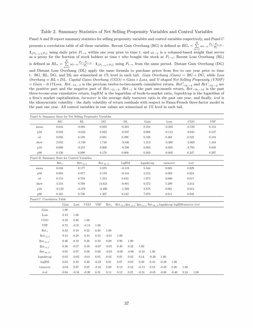
Table 2. Summary Statistics of Net Selling Propensity Variables and Control Variables

Panel A and B report summary statistics for selling propensity variables and control variables respectively, and Panel C

presents a correlation table of all these variables. Recent Gain Overhang (RG) is defined as RGt =N∑

n=1

ωt−nPt−Pt−n

Pt·

1{Pt−n≤Pt} using daily price Pt−n within one year prior to time t, and ωt−n is a volumed-based weight that servesas a proxy for the fraction of stock holders at time t who bought the stock at Pt−n; Recent Loss Overhang (RL)

is defined as RLt =N∑

n=1

ωt−nPt−Pt−n

Pt· 1{Pt−n>Pt} using Pt−n from the same period. Distant Gain Overhang (DG)

and Distant Loss Overhang (DL) apply the same formula to purchase prices from five to one year prior to timet. RG, RL, DG, and DL are winsorized at 1% level in each tail. Gain Overhang (Gain) = RG + DG, while LossOverhang = RL+DL. Capital Gains Overhang (CGO) = Gain+Loss, and V-shaped Net Selling Propensity (VNSP)= Gain− 0.17Loss. Ret−12,−2 is the previous twelve-to-two-month cumulative return, Ret+−12,−2 and Ret−−12,−2 arethe positive part and the negative part of Ret−12,−2, Ret−1 is the past one-month return, Ret−36,−13 is the pastthree-to-one-year cumulative return, logBM is the logarithm of book-to-market ratio, logmktcap is the logarithm ofa firm’s market capitalization, turnover is the average daily turnover ratio in the past one year, and finally, ivol isthe idiosyncratic volatility - the daily volatility of return residuals with respect to Fama-French three-factor model inthe past one year. All control variables in raw values are winsorized at 1% level in each tail.

Panel A. Summary Stats for Net Selling Propensity Variables

Panel B. Summary Stats for Control Variables

Panel C. Correlation TableGain Loss CGO VSP Ret-1 Ret-12,-2 Ret-12,-2

+Ret-12,-2- Ret-36,-13 logmktcap logBMturnover ivol

Gain 1.00Loss 0.43 1.00CGO 0.59 0.98 1.00VSP 0.72 -0.31 -0.13 1.00Ret-1 0.32 0.18 0.22 0.20 1.00

Ret-12,-2 0.44 0.28 0.34 0.24 -0.01 1.00

Ret-12,-2+ 0.46 0.19 0.26 0.33 0.00 0.90 1.00

Ret-12,-2- 0.36 0.57 0.59 -0.07 -0.05 0.49 0.32 1.00

Ret-36,-13 0.05 0.07 0.08 0.00 -0.03 -0.08 -0.06 -0.10 1.00logmktcap 0.03 -0.02 -0.01 0.05 0.02 0.05 0.02 0.14 -0.26 1.00

logBM 0.02 0.33 0.30 -0.23 0.01 0.07 0.03 0.20 0.10 -0.28 1.00turnover -0.04 0.07 0.05 -0.10 0.00 0.13 0.18 -0.13 0.18 -0.28 0.26 1.00

ivol 0.04 -0.34 -0.30 0.31 0.11 0.12 0.21 -0.31 -0.05 -0.08 -0.46 0.24 1.00

CGO VSPmean 0.044 -0.091 0.059 -0.201 0.104 -0.293 -0.189

RG RL DG DL Gain Loss0.154

p50 0.023 -0.024 0.022 -0.037 0.068 -0.112 -0.045 0.1270.468 0.522 0.104

skew 2.052 -5.738 1.748 -3.846 1.313 -3.360sd 0.056 0.189 0.081 0.396 0.108

-2.669 1.418p10 0.000 -0.251 0.000 -0.598 0.002 -0.805 -0.785 0.049p90 0.120 0.000 0.178 0.000 0.263 -0.002 0.247 0.297

ivolmean 0.016 0.177 0.378 -0.519 5.344 0.029

Ret-1 Ret-12,-2 Ret-36,-13 logBM logmktcap turnover

14.621 -0.801 0.372

0.024sd 0.154 0.703 1.254 0.842 1.974 0.017p50 0.004 0.077 0.159 -0.444 5.212

0.050

0.0050.0030.0065.2990.0010.011p90 0.165 0.730 1.307 0.442 7.970

3.213p10 -0.132 -0.378 -0.496 -1.569 2.878 0.013skew 4.554 9.769

37

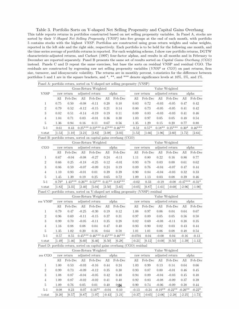
Table 3. Portfolio Sorts on V-shaped Net Selling Propensity and Capital Gains OverhangThis table reports returns in portfolios constructed based on net selling propensity variables. In Panel A, stocks aresorted by their V-Shaped Net Selling Propensity (VNSP) into five groups at the end of each month, with portfolio5 contains stocks with the highest VNSP. Portfolios are constructed using gross return weights and value weights,reported in the left side and the right side, respectively. Each portfolio is to be held for the following one month, andthe time series average of portfolio returns is reported. For each weighting scheme, I show raw portfolio returns, DGTWcharacteristic-adjusted returns, and Carhart (1997) four-factor alphas, and results in all months and in February toDecember are reported separately. Panel B presents the same set of results sorted on Capital Gains Overhang (CGO)instead. Panels C and D repeat the same exercises, but base the sorts on residual VNSP and residual CGO. Theresiduals are constructed by regressing raw net selling propensity variables (VNSP or CGO) on past returns, firmsize, turnover, and idiosyncratic volatility. The returns are in monthly percent, t-statistics for the difference betweenportfolios 5 and 1 are in the square brackets, and *, **, and *** denote significance levels at 10%, 5%, and 1%.

Panel A: portfolio return, sorted on V-shaped net selling propensity (VNSP)

VNSPAll Feb-Dec All Feb-Dec All Feb-Dec All Feb-Dec All Feb-Dec All Feb-Dec

1 0.75 0.50 -0.08 -0.11 0.20 0.10 0.83 0.72 -0.03 -0.05 0.47 0.422 0.79 0.52 -0.12 -0.15 0.21 0.14 0.80 0.73 -0.05 -0.05 0.41 0.423 0.82 0.51 -0.14 -0.19 0.19 0.11 0.89 0.83 -0.03 -0.03 0.41 0.464 1.04 0.71 0.03 -0.01 0.36 0.30 1.03 0.97 0.05 0.05 0.48 0.545 1.36 0.94 0.16 0.11 0.67 0.56 1.35 1.29 0.15 0.20 0.77 0.88

5-1 0.61 0.43 0.25*** 0.22*** 0.47*** 0.46*** 0.52 0.57* 0.18** 0.25*** 0.30* 0.46***t-stat [1.53] [1.10] [3.21] [2.82] [3.08] [3.03] [1.52] [1.66] [1.96] [2.60] [1.72] [2.64]

Panel B: portfolio return, sorted on capital gains overhang (CGO)

CGOAll Feb-Dec All Feb-Dec All Feb-Dec All Feb-Dec All Feb-Dec All Feb-Dec

1 0.67 -0.04 -0.08 -0.27 0.24 -0.11 1.11 0.80 0.22 0.16 0.86 0.772 0.66 0.25 -0.18 -0.25 0.12 -0.01 0.93 0.78 0.03 0.00 0.61 0.623 0.86 0.59 -0.07 -0.09 0.24 0.19 0.89 0.76 -0.04 -0.07 0.47 0.444 1.10 0.93 -0.01 0.01 0.39 0.39 0.90 0.84 -0.04 -0.03 0.32 0.335 1.45 1.39 0.19 0.25 0.65 0.72 1.09 1.13 0.03 0.08 0.39 0.46

5-1 0.79* 1.43*** 0.26** 0.52*** 0.41** 0.83*** -0.02 0.33 -0.19 -0.08 -0.47*** -0.31*t-stat [1.82] [3.35] [2.40] [5.04] [2.50] [5.65] [-0.05] [0.87] [-1.61] [-0.68] [-2.96] [-1.90]

Panel C: portfolio return, sorted on V-shaped net selling propensity (VNSP) residual

res VNSPAll Feb-Dec All Feb-Dec All Feb-Dec All Feb-Dec All Feb-Dec All Feb-Dec

1 0.79 0.47 -0.25 -0.30 0.19 0.12 1.08 0.97 0.06 0.04 0.64 0.672 0.96 0.69 -0.11 -0.15 0.37 0.31 0.97 0.89 0.05 0.05 0.56 0.583 0.99 0.70 -0.05 -0.11 0.35 0.28 0.82 0.69 -0.08 -0.11 0.38 0.354 1.16 0.88 0.08 0.04 0.47 0.40 0.93 0.90 0.02 0.03 0.43 0.445 1.35 1.02 0.20 0.16 0.64 0.58 1.01 1.01 0.06 0.08 0.48 0.54

5-1 0.57 0.55 0.45*** 0.46*** 0.45*** 0.46*** -0.0701 0.04 -0.00 0.04 -0.16 -0.13t-stat [1.49] [1.46] [6.60] [6.46] [6.50] [6.28] [-0.21] [0.12] [-0.00] [0.50] [-1.39] [-1.12]

Panel D: portfolio return, sorted on capital gains overhang (CGO) residual

res CGOAll Feb-Dec All Feb-Dec All Feb-Dec All Feb-Dec All Feb-Dec All Feb-Dec

1 1.00 0.53 -0.03 -0.16 0.44 0.24 1.03 0.99 0.13 0.14 0.64 0.662 0.99 0.73 -0.09 -0.12 0.35 0.30 0.93 0.87 0.00 -0.01 0.46 0.453 1.08 0.87 -0.04 -0.05 0.42 0.40 0.94 0.89 -0.04 -0.03 0.45 0.484 1.09 0.87 -0.02 -0.02 0.41 0.40 0.92 0.83 -0.08 -0.09 0.37 0.395 1.09 0.76 0.05 0.01 0.40 0.34 0.90 0.74 -0.06 -0.09 0.38 0.44

5-1 0.08 0.23 0.07 0.16** -0.04 0.10 -0.13 -0.24 -0.19** -0.22** -0.26** -0.22*t-stat [0.20] [0.57] [0.87] [1.97] [-0.43] [1.21] [-0.37] [-0.65] [-2.06] [-2.28] [-2.25] [-1.73]

Gross-Return Weighted Value Weightedraw return adjusted return alpha raw return adjusted return alpha

Gross-Return Weighted Value Weightedraw return adjusted return alpha raw return adjusted return alpha

Gross-Return Weighted Value Weightedraw return adjusted return alpha raw return adjusted return alpha

Gross-Return Weighted Value Weightedraw return adjusted return alpha raw return adjusted return alpha

38

Table 4. Predicting Returns with Gain and Loss Overhang, Fama-MacBeth Regressions

This table reports results for predictive Fama-MacBeth (1973) regressions of one-month return on lagged gain and lossoverhang variables and a set of control variables. The dependent variable is return in month t, and the explanatoryvariables are available at the end of month t-1. Gain and Loss are gain overhang and loss overhang defined in equation(1) and (2). Ret+−12,−2 and Ret−−12,−2 are the positive part and the negative part of the previous twelve-to-two-monthcumulative return, Ret−1 is the past one-month return, Ret−36,−13 is the past three-to-one-year cumulative return,logBM is the logarithm of book-to-market ratio, logmktcap is the logarithm of a firm’s market capitalization, turnoveris the average daily turnover ratio in the past one year, and ivol is idiosyncratic volatility, the daily volatility of returnresiduals with respect to Fama-French three-factor model in the past one year. Cross-sectional WLS regressions arerun every month with weights defined as prior-period gross returns, and the parameters and t-statistics (shown insquare brackets) are calculated using the time series of corresponding cross-sectional regression estimates. *, **, and*** denote significance levels at 10%, 5%, and 1%. R-sq is the average R2 from the cross-sectional regressions. Ireport coefficient estimates for all months and for February to December separately.

(1) (2) (3) (4) (5) (6) (7) (8) (9) (10)All Feb-Dec All Feb-Dec All Feb-Dec All Feb-Dec All Feb-Dec

Gain 0.020*** 0.027*** 0.000 0.008 0.049*** 0.055*** 0.033*** 0.036***[3.39] [4.73] [0.06] [1.60] [10.73] [12.70] [8.42] [9.29]

Loss 0.002 0.007*** -0.010*** -0.005*** -0.004*** -0.002* -0.011*** -0.009***[1.23] [4.33] [-6.71] [-3.92] [-3.90] [-1.87] [-10.66] [-8.82]

Ret-12,-2+ 0.006*** 0.005*** 0.005*** 0.006*** 0.009*** 0.010***

[3.46] [2.89] [3.47] [4.21] [6.41] [7.57]Ret-12,-2

- 0.057*** 0.059*** 0.033*** 0.034*** 0.025*** 0.029***[15.01] [14.80] [10.56] [10.78] [7.53] [8.80]

Ret-1 -0.067*** -0.062*** -0.058*** -0.053*** -0.057*** -0.049***[-18.28] [-16.52] [-15.47] [-13.83] [-14.08] [-12.51]

Ret-36,-13 -0.003*** -0.002*** -0.001** -0.001 -0.002** -0.000[-4.58] [-3.11] [-2.42] [-0.81] [-2.58] [-0.70]

logBM 0.002*** 0.002*** 0.002*** 0.002*** 0.002*** 0.001***[4.34] [3.75] [3.73] [3.09] [3.47] [2.83]

logmktcap -0.001*** -0.000 -0.001*** -0.001** -0.001*** -0.001**[-2.66] [-0.86] [-4.10] [-2.43] [-3.97] [-2.27]

ivol -0.316*** -0.400*** -0.317*** -0.403*** -0.218*** -0.325***[-6.38] [-7.95] [-6.51] [-8.16] [-4.16] [-6.22]

turnover -0.079 -0.051 -0.094 -0.062 -0.355 -0.252[-0.29] [-0.18] [-0.36] [-0.23] [-1.34] [-0.91]

constant 0.007*** 0.005** 0.010*** 0.008*** 0.017*** 0.015*** 0.020*** 0.018*** 0.022*** 0.020***[3.29] [2.40] [4.69] [3.87] [8.03] [6.76] [9.45] [8.29] [10.56] [9.35]

# of Obs 1,847,357 1,693,753 1,770,492 1,623,571 1,426,862 1,306,015 1,426,496 1,305,684 1426496 1305684R-sq 0.019 0.016 0.033 0.031 0.069 0.065 0.075 0.071 0.072 0.068

# of months 504 462 504 462 504 462 504 462 504 462

39

Table 5. Gain and Loss Effects in Recent Past and Distant Past, Fama-MacBeth Regressions

This table reports results for predictive Fama-MacBeth (1973) regressions of one-month return on selling propensityvariables and a set of control variables, with a focus of separating gains and losses that come from the recent past andthose from the distant past. The dependent variable is return in month t, and the explanatory variables are availableat the end of month t-1. RG and RL are gain and loss overhang with purchase price in the past one year, while DGand DL are gain and loss overhang calculated using purchase price in the previous one to five years. Ret+−12,−2 and

Ret−−12,−2 are the positive part and the negative part of the previous twelve-to-two-month cumulative return, Ret−1

is the past one-month return, Ret−36,−13 is the past three-to-one-year cumulative return, logBM is the logarithmof book-to-market ratio, logmktcap is the logarithm of a firm’s market capitalization, turnover is the average dailyturnover ratio in the past one year, and ivol is idiosyncratic volatility, the daily volatility of return residuals withrespect to Fama-French three-factor model in the past one year. Cross-sectional WLS regressions are run every monthwith weights defined as prior-period gross returns, and the parameters and t-statistics (shown in square brackets) arecalculated using the time series of corresponding cross-sectional regression estimates. *, **, and *** denote significancelevels at 10%, 5%, and 1%. R-sq is the average R2 from the cross-sectional regressions. I report coefficient estimatesfor all months and for February to December separately.

(1) (2) (3) (4) (5) (6) (7) (8)All Feb-Dec All Feb-Dec All Feb-Dec All Feb-Dec

RG -0.042*** -0.033** -0.075*** -0.061*** 0.113*** 0.129*** 0.079*** 0.091***[-2.73] [-2.15] [-4.73] [-4.01] [8.67] [9.74] [5.96] [6.72]

RL 0.017*** 0.021*** -0.003 -0.000 -0.004 -0.005 -0.014*** -0.016***[2.83] [3.38] [-0.65] [-0.04] [-1.05] [-1.31] [-4.18] [-4.59]

DG 0.036*** 0.041*** 0.018*** 0.023*** 0.029*** 0.032*** 0.022*** 0.022***[7.33] [8.26] [4.06] [5.33] [6.73] [7.11] [5.53] [5.50]

DL -0.001 0.004*** -0.011*** -0.006*** -0.003** -0.000 -0.009*** -0.007***[-0.55] [2.77] [-7.20] [-4.48] [-2.56] [-0.11] [-8.05] [-6.04]

Ret-12,-2+ 0.007*** 0.007*** 0.003** 0.004***

[5.13] [4.46] [2.21] [2.78]Ret-12,-2

- 0.055*** 0.057*** 0.034*** 0.036***[17.23] [17.26] [11.61] [12.11]

Ret-1 -0.071*** -0.067*** -0.060*** -0.054***[-20.27] [-18.38] [-16.88] [-15.07]

Ret-36,-13 -0.002*** -0.002*** -0.001** -0.001[-4.09] [-2.68] [-2.42] [-0.86]

logBM 0.002*** 0.002*** 0.002*** 0.002***[4.30] [3.69] [3.75] [3.09]

logmktcap -0.001*** -0.000* -0.001*** -0.001***[-3.52] [-1.78] [-4.71] [-3.10]

ivol -0.344*** -0.433*** -0.331*** -0.419***[-6.90] [-8.56] [-6.73] [-8.43]

turnover -0.512* -0.545* -0.430* -0.463*[-1.94] [-1.96] [-1.67] [-1.70]

constant 0.008*** 0.006*** 0.010*** 0.008*** 0.020*** 0.017*** 0.022*** 0.019***[4.11] [3.12] [5.12] [4.23] [9.07] [7.88] [10.24] [9.16]

# of Obs 1,847,357 1,693,753 1,770,492 1,623,571 1,426,862 1,306,015 1,426,496 1,305,684R-sq 0.033 0.030 0.042 0.040 0.073 0.068 0.078 0.074

# of months 504 462 504 462 504 462 504 462

40

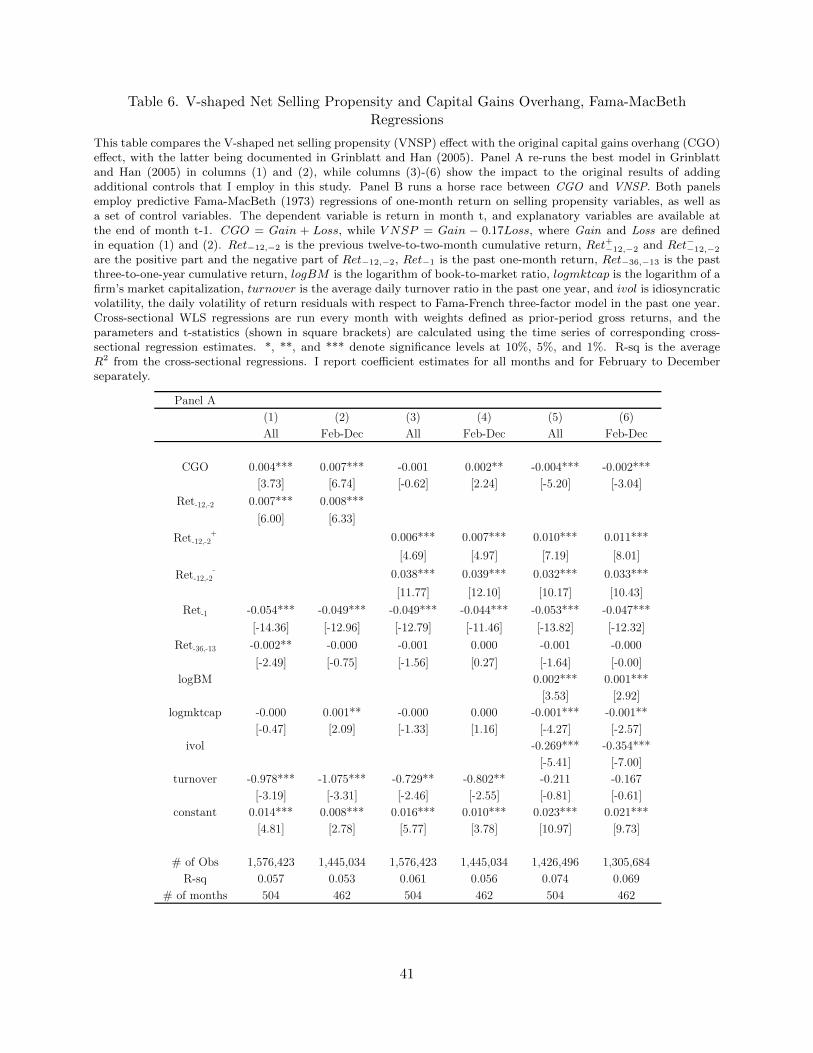
Table 6. V-shaped Net Selling Propensity and Capital Gains Overhang, Fama-MacBethRegressions

This table compares the V-shaped net selling propensity (VNSP) effect with the original capital gains overhang (CGO)effect, with the latter being documented in Grinblatt and Han (2005). Panel A re-runs the best model in Grinblattand Han (2005) in columns (1) and (2), while columns (3)-(6) show the impact to the original results of addingadditional controls that I employ in this study. Panel B runs a horse race between CGO and VNSP. Both panelsemploy predictive Fama-MacBeth (1973) regressions of one-month return on selling propensity variables, as well asa set of control variables. The dependent variable is return in month t, and explanatory variables are available atthe end of month t-1. CGO = Gain + Loss, while V NSP = Gain − 0.17Loss, where Gain and Loss are definedin equation (1) and (2). Ret−12,−2 is the previous twelve-to-two-month cumulative return, Ret+−12,−2 and Ret−−12,−2

are the positive part and the negative part of Ret−12,−2, Ret−1 is the past one-month return, Ret−36,−13 is the pastthree-to-one-year cumulative return, logBM is the logarithm of book-to-market ratio, logmktcap is the logarithm of afirm’s market capitalization, turnover is the average daily turnover ratio in the past one year, and ivol is idiosyncraticvolatility, the daily volatility of return residuals with respect to Fama-French three-factor model in the past one year.Cross-sectional WLS regressions are run every month with weights defined as prior-period gross returns, and theparameters and t-statistics (shown in square brackets) are calculated using the time series of corresponding cross-sectional regression estimates. *, **, and *** denote significance levels at 10%, 5%, and 1%. R-sq is the averageR2 from the cross-sectional regressions. I report coefficient estimates for all months and for February to Decemberseparately.

Panel A(1) (2) (3) (4) (5) (6)All Feb-Dec All Feb-Dec All Feb-Dec

CGO 0.004*** 0.007*** -0.001 0.002** -0.004*** -0.002***[3.73] [6.74] [-0.62] [2.24] [-5.20] [-3.04]

Ret-12,-2 0.007*** 0.008***[6.00] [6.33]

Ret-12,-2+ 0.006*** 0.007*** 0.010*** 0.011***

[4.69] [4.97] [7.19] [8.01]Ret-12,-2

- 0.038*** 0.039*** 0.032*** 0.033***[11.77] [12.10] [10.17] [10.43]

Ret-1 -0.054*** -0.049*** -0.049*** -0.044*** -0.053*** -0.047***[-14.36] [-12.96] [-12.79] [-11.46] [-13.82] [-12.32]

Ret-36,-13 -0.002** -0.000 -0.001 0.000 -0.001 -0.000[-2.49] [-0.75] [-1.56] [0.27] [-1.64] [-0.00]

logBM 0.002*** 0.001***[3.53] [2.92]

logmktcap -0.000 0.001** -0.000 0.000 -0.001*** -0.001**[-0.47] [2.09] [-1.33] [1.16] [-4.27] [-2.57]

ivol -0.269*** -0.354***[-5.41] [-7.00]

turnover -0.978*** -1.075*** -0.729** -0.802** -0.211 -0.167[-3.19] [-3.31] [-2.46] [-2.55] [-0.81] [-0.61]

constant 0.014*** 0.008*** 0.016*** 0.010*** 0.023*** 0.021***[4.81] [2.78] [5.77] [3.78] [10.97] [9.73]

# of Obs 1,576,423 1,445,034 1,576,423 1,445,034 1,426,496 1,305,684R-sq 0.057 0.053 0.061 0.056 0.074 0.069

# of months 504 462 504 462 504 462

41

(Table 6 Continued)Panel B

(1) (2) (3) (4) (5) (6) (7) (8)All Feb-Dec All Feb-Dec All Feb-Dec All Feb-Dec

CGO 0.005*** 0.010*** -0.008*** -0.003*** 0.003*** 0.006*** -0.004*** -0.002**[2.98] [7.17] [-5.56] [-2.59] [2.87] [5.78] [-4.60] [-2.45]

VNSP 0.016*** 0.017*** 0.009* 0.011** 0.046*** 0.049*** 0.037*** 0.038***[2.81] [3.13] [1.71] [2.43] [11.48] [12.59] [10.38] [10.61]

Ret-12,-2+ 0.006*** 0.005*** 0.005*** 0.006***

[3.46] [2.89] [3.47] [4.21]Ret-12,-2

- 0.057*** 0.059*** 0.033*** 0.034***[15.01] [14.80] [10.56] [10.78]

Ret-1 -0.067*** -0.062*** -0.058*** -0.053***[-18.28] [-16.52] [-15.47] [-13.83]

Ret-36,-13 -0.003*** -0.002*** -0.001** -0.001[-4.58] [-3.11] [-2.42] [-0.81]

logBM 0.002*** 0.002*** 0.002*** 0.002***[4.34] [3.75] [3.73] [3.09]

logmktcap -0.001*** -0.000 -0.001*** -0.001**[-2.66] [-0.86] [-4.10] [-2.43]

ivol -0.316*** -0.400*** -0.317*** -0.403***[-6.38] [-7.95] [-6.51] [-8.16]

turnover -0.079 -0.051 -0.094 -0.062[-0.29] [-0.18] [-0.36] [-0.23]

constant 0.007*** 0.005** 0.010*** 0.008*** 0.017*** 0.015*** 0.020*** 0.018***[3.29] [2.40] [4.69] [3.87] [8.03] [6.76] [9.45] [8.29]

# of Obs 1,847,357 1,693,753 1,770,492 1,623,571 1,426,862 1,306,015 1,426,496 1,305,684R-sq 0.019 0.016 0.033 0.031 0.069 0.065 0.075 0.071

# of months 504 462 504 462 504 462 504 462

42

Tab

le7.

Gain

and

Los

sE

ffec

tsin

Su

bsa

mp

les,

Fam

a-M

acB

eth

Reg

ress

ion

s

This

table

rep

ort

sre

sult

sfo

rpre

dic

tive

Fam

a-M

acB

eth

(1973)

regre

ssio

ns

of

one-

month

retu

rnon

lagged

gain

and

loss

over

hang

vari

able

sand

ase

tof

contr

ol

vari

able

sin

cross

-sec

tional

subsa

mple

s.

The

subsa

mple

sare

const

ruct

edbase

don

inst

ituti

onal

owner

ship

,firm

size

,tu

rnov

erra

tio

and

stock

vola

tility

.E

xce

pt

for

firm

size

subsa

mple

s,all

oth

er“hig

h”

gro

ups

conta

inth

eto

p1/3

of

firm

sin

the

whole

sam

ple

ranked

on

the

cate

gori

zing

vari

able

,w

hile

the

“lo

w”

gro

ups

corr

esp

ond

toth

eb

ott

om

1/3

of

firm

s.A

sfo

rsi

ze,

“hig

h”

and

“lo

w”

gro

ups

are

div

ided

by

NY

SE

bre

ak

poin

tsw

hic

hco

rres

pond

toth

eto

p30%

and

the

bott

om

30%

of

NY

SE

firm

s.T

he

dep

enden

tva

riable

isre

turn

inm

onth

t,and

the

expla

nato

ryva

riable

sare

available

at

the

end

of

month

t-1.Gain

andLoss

are

gain

over

hang

and

loss

over

hang

defi

ned

ineq

uati

on

(1)

and

(2).

Ret

+ −12,−

2and

Ret− −12,−

2are

the

posi

tive

part

and

the

neg

ati

ve

part

of

the

pre

vio

us

twel

ve-

to-t

wo-m

onth

cum

ula

tive

retu

rn,Ret−1

isth

epast

one-

month

retu

rn,Ret−36,−

13

isth

epast

thre

e-to

-one-

yea

rcu

mula

tive

retu

rn,logBM

isth

elo

gari

thm

of

book-t

o-m

ark

etra

tio,logmktcap

isth

elo

gari

thm

of

afirm

’sm

ark

etca

pit

aliza

tion,turn

over

isth

eav

erage

daily

turn

over

rati

oin

the

past

one

yea

r,andivol

isid

iosy

ncr

ati

cvola

tility

,th

edaily

vola

tility

of

retu

rnre

siduals

wit

hre

spec

tto

Fam

a-F

rench

thre

e-fa

ctor

model

inth

epast

one

yea

r.C

ross

-sec

tional

regre

ssio

ns

are

run

ever

ym

onth

,and

the

para

met

ers

and

t-st

ati

stic

s(s

how

nin

square

bra

cket

s)are

calc

ula

ted

usi

ng

the

tim

ese

ries

of

corr

esp

ondin

gcr

oss

-sec

tional

regre

ssio

nes

tim

ate

s.*,

**,

and

***

den

ote

signifi

cance

level

sat

10%

,5%

,and

1%

.R

-sq

isth

eav

erageR

2fr

om

the

cross

-sec

tional

regre

ssio

ns.

Ire

port

coeffi

cien

tes

tim

ate

sfo

rall

month

sand

for

Feb

ruary

toD

ecem

ber

separa

tely

.

(1)

(2)

(3)

(4)

(5)

(6)

(7)

(8)

All

Feb-

Dec

All

Feb-

Dec

All

Feb-

Dec

All

Feb-

Dec

All

Feb-

Dec

All

Feb-

Dec

Gai

n0.

026*

**0.

030*

**0.

035*

**0.

037*

**-0

.007

-0.0

07-0

.007

-0.0

020.

054*

**0.

057*

**0.

061*

**0.

059*

**[4

.67]

[5.0

5][7

.31]

[7.4

5][-0

.60]

[-0.4

2][-1

.26]

[-0.3

5][1

0.33

][1

0.85

][-8

.95]

[-8.7

4]Lo

ss-0

.012

***

-0.0

10**

*-0

.012

***

-0.0

10**

*0.

000

0.00

0-0

.007

***

-0.0

08**

*-0

.011

***

-0.0

09**

*0.

004*

0.00

1[-7

.05]

[-5.7

5][-6

.69]

[-5.4

0][0

.09]

[0.1

2][-4

.46]

[-5.0

1][-9

.13]

[-7.3

8][1

.85]

[0.4

2]R

et-1

2,-2

+0.

006*

**0.

006*

**0.

003*

*0.

003*

**0.

009*

**0.

009*

**0.

001

0.00

2*[3

.61]

[3.8

5][2

.23]

[2.6

2][4

.41]

[4.3

8][1

.14]

[1.8

0]R

et-1

2,-2

-0.

026*

**0.

026*

**0.

035*

**0.

038*

**0.

018*

**0.

020*

**0.

037*

**0.

037*

**[5

.85]

[5.6

6][8

.10]

[8.7

5][3

.22]

[3.3

5][1

2.04

][1

1.95

]R

et-1

-0.0

46**

*-0

.041

***

-0.0

36**

*-0

.034

***

-0.0

31**

*-0

.025

***

-0.0

60**

*-0

.056

***

[-10.

71]

[-9.3

7][-8

.67]

[-7.7

0][-5

.60]

[-4.4

1][-1

6.11

][-1

4.98

]R

et-3

6,-1

3-0

.001

**-0

.001

-0.0

01*

-0.0

00-0

.000

0.00

1-0

.002

***

-0.0

01**

[-1.9

8][-1

.24]

[-1.6

7][-0

.31]

[-0.1

1][0

.86]

[-3.2

5][-2

.02]

logB

M0.

000

0.00

00.

002*

**0.

002*

**0.

001

0.00

00.

002*

**0.

002*

**[0

.21]

[0.2

1][3

.42]

[3.5

2][0

.88]

[0.0

7][3

.94]

[3.7

1]lo

gmkt

cap

-0.0

01-0

.000

-0.0

01**

-0.0

00-0

.001

**-0

.001

**-0

.001

*-0

.000

[-1.5

1][-0

.75]

[-2.1

8][-0

.87]

[-2.2

9][-2

.57]

[-1.8

3][-0

.08]

ivol

-0.1

39**

*-0

.202

***

-0.2

57**

*-0

.312

***

-0.2

54**

-0.3

81**

*-0

.268

***

-0.3

35**

*[-2

.59]

[-3.6

7][-5

.18]

[-6.1

4][-2

.33]

[-3.4

5][-5

.96]

[-7.2

7]tu

rnov

er0.

351*

0.36

5*-0

.827

***

-1.0

39**

*-0

.447

-0.3

82-0

.287

-0.2

61[1

.84]

[1.8

2][-4

.07]

[-5.2

1][-1

.21]

[-1.0

1][-1

.17]

[-1.0

0]co

nsta

nt0.

012*

**0.

010*

**0.

017*

**0.

015*

**0.

019*

**0.

021*

**0.

018*

**0.

013*

**[4

.09]

[3.4

6][7

.31]

[6.5

0][4

.78]

[5.1

6][7

.07]

[5.1

3]

# o

f Obs

430,

356

393,

733

357,

731

327,

562

227,

350

208,

114

820,

261

751,

108

R-s

q0.

070

0.06

80.

090

0.08

80.

153

0.15

00.

065

0.06

2#

of m

onth

s38

435

238

435

250

446

250

446

2

Inst

Ow

n H

igh

Inst

Ow

n Lo

wH

ighβ

- Low

βM

ktca

p H

igh

Mkt

cap

Low

Hig

hβ- L

owβ

43

(Tab

le 7

Con

tinue

d)(9

)(1

0)(1

1)(1

2)(1

3)(1

4)(1

5)(1

6)

All

Feb-

Dec

All

Feb-

Dec

All

Feb-

Dec

All

Feb-

Dec

All

Feb-

Dec

All

Feb-

Dec

Gai

n0.

049*

**0.

054*

**0.

019*

**0.

018*

**0.

030*

**0.

036*

**0.

051*

**0.

054*

**0.

014*

**0.

016*

**0.

037*

**0.

038*

**[8

.40]

[9.1

9][3

.99]

[3.8

0][5

.05]

[5.8

2][8

.55]

[8.9

6][3

.79]

[4.0

1][5

.82]

[6.0

3]Lo

ss-0

.017

***

-0.0

16**

*-0

.007

***

-0.0

04**

*-0

.010

***

-0.0

12**

*-0

.012

***

-0.0

10**

*-0

.007

***

-0.0

05**

*-0

.005

***

-0.0

05**

*[-1

0.62

][-9

.38]

[-6.1

8][-4

.16]

[-6.4

2][-6

.56]

[-8.7

5][-7

.07]

[-5.9

4][-4

.49]

[-3.9

7][-3

.48]

Ret

-12,

-2+

0.00

20.

003*

*0.

006*

**0.

007*

**0.

001

0.00

2*0.

006*

**0.

008*

**[1

.55]

[2.1

2][3

.19]

[4.0

2][1

.20]

[1.6

6][2

.83]

[3.7

6]R

et-1

2,-2

-0.

035*

**0.

034*

**0.

034*

**0.

037*

**0.

036*

**0.

036*

**0.

027*

**0.

030*

**[9

.36]

[9.2

6][8

.24]

[8.6

1][9

.14]

[9.0

0][6

.85]

[7.4

1]R

et-1

-0.0

39**

*-0

.035

***

-0.0

78**

*-0

.071

***

-0.0

47**

*-0

.043

***

-0.0

67**

*-0

.059

***

[-10.

15]

[-9.0

4][-1

7.90

][-1

6.33

][-1

2.86

][-1

1.68

][-1

5.80

][-1

3.95

]R

et-3

6,-1

3-0

.001

**-0

.000

-0.0

000.

001

-0.0

01*

-0.0

000.

001

0.00

1**

[-2.2

7][-0

.97]

[-0.5

0][1

.20]

[-1.9

6][-0

.40]

[1.0

3][2

.25]

logB

M0.

002*

*0.

001*

0.00

2***

0.00

2***

0.00

2***

0.00

2***

0.00

2***

0.00

1**

[2.5

0][1

.92]

[3.6

7][2

.86]

[3.7

7][3

.32]

[3.4

7][2

.42]

logm

ktca

p-0

.001

***

-0.0

01-0

.001

**-0

.000

-0.0

01**

*-0

.001

-0.0

00-0

.000

[-2.9

6][-1

.59]

[-2.4

9][-0

.82]

[-2.7

0][-1

.37]

[-1.5

2][-0

.13]

ivol

-0.4

47**

*-0

.525

***

-0.1

30**

-0.2

10**

*-0

.378

***

-0.4

33**

*0.

056

-0.0

52[-8

.48]

[-9.8

1][-2

.53]

[-4.0

0][-7

.29]

[-8.1

5][0

.73]

[-0.6

6]tu

rnov

er-0

.058

-0.0

352.

295*

*2.

212*

*-0

.189

-0.2

280.

022

-0.0

60[-0

.32]

[-0.1

8][2

.06]

[1.9

9][-0

.97]

[-1.1

1][0

.06]

[-0.1

5]co

nsta

nt0.

021*

**0.

017*

**0.

014*

**0.

012*

**0.

022*

**0.

018*

**0.

011*

**0.

010*

**[5

.94]

[4.8

5][6

.90]

[5.8

0][4

.60]

[3.6

9][5

.80]

[4.8

6]

# o

f Obs

428,

286

392,

023

502,

989

460,

502

436,

682

399,

588

494,

059

452,

396

R-s

q0.

078

0.07

30.

080

0.07

40.

075

0.07

10.

070

0.06

5#

of m

onth

s50

446

250

446

250

446

250

446

2

Tur

nove

r H

igh

Tur

nove

r Lo

wH

ighβ

- Low

βV

olat

ility

Hig

hV

olat

ility

Low

Hig

hβ- L

owβ

44

Table 8. Alternative Specifications and Alternative Samples, Fama-MacBeth Regressions

This table reports results for predictive Fama-MacBeth (1973) regressions of one-month return on lagged gain and lossoverhang variables and a set of control variables. The dependent variable is return in month t, and the explanatoryvariables are available at the end of month t-1. Gain and Loss are gain overhang and loss overhang defined in equation(1) and (2). In columns (1) and (2), Gain and Loss are constructed using prices adjusted for stock splits and dividends.In columns (3) and (4), Gain and Loss are constructed using weekly prices and volumes. In columns (5) and (6),I apply the main specifications for Gain and Loss, but the regressions are run on NYSE and AMEX stocks only.Ret+−12,−2 and Ret−−12,−2 are the positive part and the negative part of the previous twelve-to-two-month cumulativereturn, Ret−1 is the past one-month return, Ret−36,−13 is the past three-to-one-year cumulative return, logBM isthe logarithm of book-to-market ratio, logmktcap is the logarithm of a firm’s market capitalization, turnover is theaverage daily turnover ratio in the past one year, and ivol is idiosyncratic volatility, the daily volatility of returnresiduals with respect to Fama-French three-factor model in the past one year. Cross-sectional WLS regressions arerun every month with weights defined as prior-period gross returns, and the parameters and t-statistics (shown insquare brackets) are calculated using the time series of corresponding cross-sectional regression estimates. *, **, and*** denote significance levels at 10%, 5%, and 1%. R-sq is the average R2 from the cross-sectional regressions. Ireport coefficient estimates for all months and for February to December separately.

(1) (2) (3) (4) (5) (6)

All Feb-Dec All Feb-Dec All Feb-Dec

Gain 0.0332*** 0.0398*** 0.0383*** 0.0407*** 0.0197*** 0.0235***[7.44] [9.07] [9.69] [10.25] [4.49] [5.49]

Loss -0.0111*** -0.0080*** -0.0082*** -0.0063*** -0.0082*** -0.0062***[-7.75] [-5.76] [-8.36] [-6.47] [-7.23] [-5.60]

Ret-12,-2+ -0.0595*** -0.0556*** -0.0611*** -0.0549*** 0.0048*** 0.0059***

[-15.37] [-13.90] [-16.08] [-14.46] [3.23] [3.92]Ret-12,-2

- -0.0018*** -0.0013** -0.0018*** -0.0008 0.0304*** 0.0311***[-3.08] [-2.10] [-2.97] [-1.37] [8.49] [8.45]

Ret-1 0.0019*** 0.0017*** 0.0018*** 0.0015*** -0.0520*** -0.0461***[4.06] [3.62] [3.72] [3.05] [-12.32] [-10.75]

Ret-36,-13 -0.0010*** -0.0006** -0.0011*** -0.0007*** -0.0010 -0.0002[-4.01] [-2.45] [-4.29] [-2.59] [-1.57] [-0.25]

logBM -0.3105*** -0.3820*** -0.2987*** -0.3828*** 0.0018*** 0.0015***[-6.49] [-7.77] [-6.21] [-7.84] [3.69] [3.08]

logmktcap 0.0043 0.0682 -0.1178 -0.0836 -0.0010*** -0.0006**[0.02] [0.24] [-0.44] [-0.30] [-3.69] [-2.17]

ivol 0.0034*** 0.0037*** 0.0034*** 0.0045*** -0.3001*** -0.3910***[2.61] [2.65] [2.65] [3.48] [-5.41] [-6.90]

turnover 0.0324*** 0.0317*** 0.0295*** 0.0311*** -0.1031 -0.0681[9.97] [9.57] [9.37] [9.71] [-0.38] [-0.24]

constant 0.0195*** 0.0169*** 0.0199*** 0.0176*** 0.0195*** 0.0174***[9.34] [8.05] [9.72] [8.50] [8.94] [7.89]

# of Obs 1,426,496 1,305,684 1,466,316 1,341,612 823,278 754,104R-sq 0.076 0.071 0.074 0.070 0.082 0.078

# of months 504 462 504 462 504 462

adjust prices for stocksplits and dividends

aggregate prices atweekly frequency

NYSE & AMEX onlyalternative

specificationor sample:

45

Table 9. Checking Liquidity Effects, Fama-MacBeth Regressions

This table reports results for predictive Fama-MacBeth (1973) regressions of one-month return on lagged gain and lossoverhang variables and a set of control variables. The dependent variable is return in month t, and the explanatoryvariables are available at the end of month t-1. Gain and Loss are gain overhang and loss overhang defined in equation(1) and (2). In columns (1) and (2), Gain and Loss are lagged by ten days from the end of month t-1. In columns(3) and (4), Gain and Loss are lagged by one month. For columns (5)-(8), I apply the main specifications for Gainand Loss. Ret+−12,−2 and Ret−−12,−2 are the positive part and the negative part of the previous twelve-to-two-monthcumulative return, Ret−1 is the past one-month return, Ret−36,−13 is the past three-to-one-year cumulative return,logBM is the logarithm of book-to-market ratio, logmktcap is the logarithm of a firm’s market capitalization, turnoveris the average daily turnover ratio in the past one year, and ivol is idiosyncratic volatility, the daily volatility of returnresiduals with respect to Fama-French three-factor model in the past one year. Cross-sectional WLS regressions arerun every month. In columns (1)-(4), the weight is defined as prior-period gross return, and in columns (5)-(8), theweight is market capitalization of a stock. Columns (1)-(6) utilize the whole sample while columns (7)-(8) excludefirms with size that are comparable to the largest 30% of NYSE firms. The parameters and t-statistics (shown insquare brackets) are calculated using the time series of corresponding cross-sectional regression estimates. *, **, and*** denote significance levels at 10%, 5%, and 1%. R-sq is the average R2 from the cross-sectional regressions. Ireport coefficient estimates for all months and for February to December separately.

(1) (2) (3) (4) (5) (6) (7) (8)

All Feb-Dec All Feb-Dec All Feb-Dec All Feb-Dec

Gain 0.038*** 0.039*** 0.013*** 0.015*** -0.003 0.001 0.019*** 0.019***[9.59] [9.91] [3.75] [4.35] [-0.55] [0.10] [3.93] [4.46]

Loss -0.004*** -0.003** -0.005*** -0.003*** -0.006*** -0.005*** -0.010*** -0.009***[-4.13] [-2.54] [-5.45] [-3.49] [-4.37] [-4.06] [-8.74] [-7.38]

Ret-12,-2+ 0.003*** 0.005*** 0.007*** 0.009*** 0.010*** 0.011*** 0.008*** 0.009***

[2.72] [3.80] [5.96] [6.77] [5.07] [5.45] [5.01] [5.52]Ret-12,-2

- 0.024*** 0.026*** 0.029*** 0.030*** 0.014*** 0.017*** 0.020*** 0.021***[7.84] [8.41] [9.41] [9.56] [3.20] [3.68] [5.46] [5.79]

Ret-1 -0.063*** -0.056*** -0.056*** -0.048*** -0.033*** -0.027*** -0.044*** -0.040***[-16.27] [-14.67] [-13.88] [-12.21] [-6.07] [-4.91] [-10.85] [-9.43]

Ret-36,-13 -0.002*** -0.001* -0.001** -0.000 0.000 0.001 -0.001 0.000[-3.59] [-1.94] [-2.29] [-0.69] [0.11] [1.26] [-1.04] [0.57]

logBM 0.002*** 0.001*** 0.002*** 0.001*** 0.001 0.001 0.002*** 0.001**[3.62] [2.95] [3.36] [2.67] [1.58] [0.82] [3.09] [2.29]

logmktcap -0.001*** -0.001** -0.001*** -0.001** -0.001*** -0.001*** -0.001** -0.000[-3.89] [-2.21] [-4.13] [-2.47] [-3.25] [-3.73] [-2.11] [-0.91]

ivol -0.259*** -0.348*** -0.272*** -0.358*** -0.341*** -0.452*** -0.355*** -0.431***[-5.27] [-7.04] [-5.51] [-7.17] [-4.28] [-5.62] [-5.57] [-6.55]

turnover -0.214 -0.172 -0.223 -0.196 -0.557* -0.598* -0.106 -0.166[-0.82] [-0.62] [-0.86] [-0.72] [-1.70] [-1.79] [-0.45] [-0.67]

constant 0.019*** 0.017*** 0.021*** 0.019*** 0.021*** 0.023*** 0.019*** 0.017***[9.14] [8.00] [10.02] [8.84] [6.14] [6.56] [6.72] [5.97]

# of Obs 1,425,623 1,304,873 1,404,236 1,285,340 1,426,496 1,305,684 1,199,146 1,097,570R-sq 0.075 0.071 0.075 0.070 0.157 0.153 0.090 0.088

# of months 504 462 503 461 504 462 504 462

Lag Gain & Lossby 10 days

Lag Gain & Lossby 1 month

Value weightedValue weighted, excluding

mega-sized firms

46

Table 10. Checking Impacts of Short-Sale Constraint, Fama-MacBeth Regressions

This table reports results for predictive Fama-MacBeth (1973) regressions of one-month return on lagged gain and lossoverhang variables and a set of control variables. The dependent variable is return in month t, and the explanatoryvariables are available at the end of month t-1. Gain and Loss are gain overhang and loss overhang defined in equation(1) and (2). Ret+−12,−2 and Ret−−12,−2 are the positive part and the negative part of the previous twelve-to-two-monthcumulative return, Ret−1 is the past one-month return, Ret−36,−13 is the past three-to-one-year cumulative return,logBM is the logarithm of book-to-market ratio, logmktcap is the logarithm of a firm’s market capitalization, turnoveris the average daily turnover ratio in the past one year, and ivol is idiosyncratic volatility, the daily volatility of returnresiduals with respect to Fama-French three-factor model in the past one year. Columns (1)-(2) exclude stocks whoseinstitutional ownership are ranked at the bottom 1/3 and short interest ratio areranked among the top 5%. Columns(3)-(4) exclude stocks whose institutional ownership are ranked at the bottom 1/3 and short interest ratio are greaterthan or equal to 2.5%. Columns (5)-(8) repeat these restrictions and conduct regressions in the subsample from 2003Jul to 2011 Dec. Cross-sectional WLS regressions are run every month where the weights are defined as prior-periodgross returns. The parameters and t-statistics (shown in square brackets) are calculated using the time series ofcorresponding cross-sectional regression estimates. *, **, and *** denote significance levels at 10%, 5%, and 1%. R-sqis the average R2 from the cross-sectional regressions. I report coefficient estimates for all months and for Februaryto December separately.

(1) (2) (3) (4) (5) (6) (7) (8)

All Feb-Dec All Feb-Dec All Feb-Dec All Feb-Dec

Gain 0.033*** 0.036*** 0.033*** 0.036*** 0.034*** 0.039*** 0.034*** 0.040***[7.69] [7.94] [7.37] [7.70] [3.26] [3.49] [2.93] [3.26]

Loss -0.011*** -0.009*** -0.011*** -0.009*** -0.006** -0.003 -0.005* -0.002[-8.92] [-7.27] [-8.56] [-6.90] [-2.40] [-1.21] [-1.82] [-0.62]

Ret-12,-2+ 0.003*** 0.004*** 0.003*** 0.004*** -0.001 -0.001 -0.001 0.000

[3.51] [4.34] [3.70] [4.58] [-0.66] [-0.27] [-0.36] [0.10]Ret-12,-2

- 0.031*** 0.033*** 0.031*** 0.032*** 0.012 0.012 0.012 0.012[8.83] [8.86] [8.82] [8.72] [1.41] [1.36] [1.46] [1.29]

Ret-1 -0.039*** -0.035*** -0.039*** -0.035*** -0.022*** -0.016* -0.021*** -0.016*[-11.58] [-10.07] [-11.44] [-9.99] [-2.73] [-1.95] [-2.63] [-1.90]

Ret-36,-13 -0.001** -0.001 -0.001** -0.001 -0.001 -0.001 -0.002 -0.001[-2.29] [-1.21] [-2.35] [-1.35] [-1.15] [-0.94] [-1.18] [-1.06]

logBM 0.001** 0.001** 0.001** 0.001** 0.000 0.000 -0.000 -0.000[2.55] [2.47] [2.30] [2.18] [0.39] [0.42] [-0.21] [-0.25]

logmktcap -0.001** -0.000 -0.001** -0.000 -0.000 -0.000 -0.000 -0.000[-2.39] [-1.30] [-2.40] [-1.28] [-0.61] [-0.35] [-0.73] [-0.41]

ivol -0.225*** -0.289*** -0.217*** -0.280*** -0.116 -0.166* -0.082 -0.131[-4.98] [-6.29] [-4.83] [-6.12] [-1.37] [-1.95] [-0.99] [-1.58]

turnover -0.045 -0.107 -0.049 -0.112 0.015 0.005 0.067 0.060[-0.26] [-0.60] [-0.28] [-0.63] [0.12] [0.03] [0.50] [0.42]

constant 0.016*** 0.015*** 0.016*** 0.015*** 0.005 0.006 0.005 0.005[6.84] [6.10] [6.74] [5.94] [1.31] [1.44] [1.14] [1.16]

# of Obs 1,203,983 1,101,849 1,155,925 1,057,830 331,567 302,270 291,346 265,421R-sq 0.065 0.062 0.064 0.062 0.051 0.048 0.050 0.047

# of months 384 352 384 352 102 93 102 93

1980 Jan - 2011 Dec 2003 Jul - 2011 Decexcluding stocks

IO<p33 & SI≥p95excluding stocks

IO<p33 & SI≥2.5%excluding stocks

IO<p33 & SI≥p95excluding stocks

IO<p33 & SI≥2.5%

47

Appendix

A. Time-series Variation: the Impact of Capital Gains Tax

I here test additional pricing implications of investors’ trading behavior. If the return predictability

shown in section 4 really comes from investors’ trading behavior rather other mechanisms, as people’s

trading incentives change over time, so should the aggregate gain and loss effects. I particularly

examine how capital gains tax change in the 40 years of this study period lead to variation in the

gain and loss effects. Capital gains tax, as shown in the literature (e.g., Odean (1998), Lakonishok

and Smidt (1986), Ben-David and Hirshleifer (2012)), is not a major source of the (V-shaped)

disposition effect; however, it has incremental impact on people’s selling behavior. Moreover, what

makes it a good test for my purpose is that tax incentive has different implications for the gain side

versus the loss side. When capital gains tax is higher, investors are less willing to realize a gain since

they have to pay more tax; on the loss side, they would be more willing to sell because the realized

loss can offset gains earned elsewhere. Thus the price-level implication is that in high tax periods,

the gain effect should be lessened, while the loss effect should be amplified. Please note that this

variation is not a unique prediction of the V-shaped selling schedule - a monotonic selling schedule

predicts the same pattern. This exercise does not attempt to distinguish the shape of investors’

selling schedule, rather, it is designed to discriminate the source of return predictability on a more

general level: whether the observed return pattern is a consequence of trading behavior in general,

or it is a result of other factors, such as risk.

Capital gains tax rate in the United States depends on the holding period of the gain: if it’s a

short-term gain (which generally means shorter than one year), investors pay the tax rate of their

ordinary income tax; if it’s a long-term gain, investors pay a capital gains tax rate that is lower than

their income tax. The capital gains tax rate that applies to an investor also depends on his or her

ordinary income tax. Given the heterogeneity in investors’ income distribution and holding period,

it is hard to capture the accurate effective tax rate that applies to a representative investor. Thus,

instead of employing a continuous tax rate variable, I use the maximum capital gains tax rate as

an indicator to see if tax is relatively high or low in a given period. There are significant changes

in tax regimes for the period of my sample (Figure 2): the top capital gains tax rate starts at 32%

in 1970, increases to around 40% in 1976, then drops to 20% in the early 1980s; it then increases

to 29% in 1987 but falls to below 20% and remain there since 2003. I group all months that have

a tax rate higher than 25% (the median rate) into a high tax subsample, while months with a tax

48

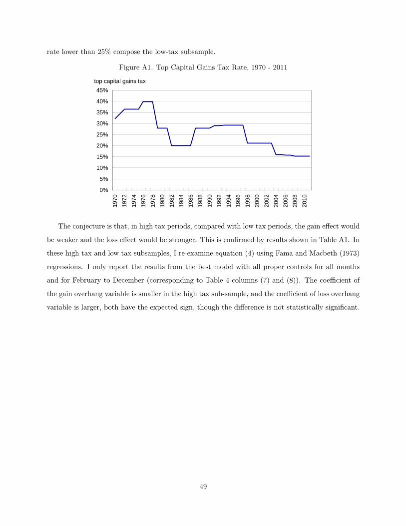
rate lower than 25% compose the low-tax subsample.

Figure A1. Top Capital Gains Tax Rate, 1970 - 2011

top capital gains tax

0%

5%

10%

15%

20%

25%

30%

35%

40%

45%

1970

1972

1974

1976

1978

1980

1982

1984

1986

1988

1990

1992

1994

1996

1998

2000

2002

2004

2006

2008

2010

The conjecture is that, in high tax periods, compared with low tax periods, the gain effect would

be weaker and the loss effect would be stronger. This is confirmed by results shown in Table A1. In

these high tax and low tax subsamples, I re-examine equation (4) using Fama and Macbeth (1973)

regressions. I only report the results from the best model with all proper controls for all months

and for February to December (corresponding to Table 4 columns (7) and (8)). The coefficient of

the gain overhang variable is smaller in the high tax sub-sample, and the coefficient of loss overhang

variable is larger, both have the expected sign, though the difference is not statistically significant.

49

Table A1. Gain and Loss Effects Under Different Tax Regimes, Fama-MacBeth Regressions

This table reports results for predictive Fama-MacBeth (1973) regressions of one-month return on lagged gain andloss overhang variables and a set of control variables in subsamples based on capital gains tax rate. The high taxsub-sample contains months where the top capital gains tax rate is higher than 25%, while the low tax sub-samplecontains months where the rate is lower than 25%. The dependent variable is return in month t, and the explanatoryvariables are available at the end of month t-1. Gain and Loss are gain overhang and loss overhang defined in equation(1) and (2). Ret+−12,−2 and Ret−−12,−2 are the positive part and the negative part of the previous twelve-to-two-monthcumulative return, Ret−1 is the past one-month return, Ret−36,−13 is the past three-to-one-year cumulative return,logBM is the logarithm of book-to-market ratio, logmktcap is the logarithm of a firm’s market capitalization, turnoveris the average daily turnover ratio in the past one year, and ivol is idiosyncratic volatility, the daily volatility of returnresiduals with respect to Fama-French three-factor model in the past one year. Cross-sectional WLS regressions arerun every month with weights defined as prior-period gross returns, and the parameters and t-statistics (shown insquare brackets) are calculated using the time series of corresponding cross-sectional regression estimates. *, **, and*** denote significance levels at 10%, 5%, and 1%. R-sq is the average R2 from the cross-sectional regressions. Ireport coefficient estimates for all months and for February to December separately.

(1) (2) (3) (4) (5) (6)

All Feb-Dec All Feb-Dec All Feb-Dec

Gain 0.030*** 0.033*** 0.037*** 0.040*** -0.007 -0.007[5.44] [6.37] [6.63] [6.78] [-0.84] [-0.84]

Loss -0.011*** -0.010*** -0.010*** -0.008*** 0.001 0.002[-9.09] [-7.78] [-6.10] [-4.82] [0.69] [0.87]

Ret-12,-2+ 0.006*** 0.008*** 0.002 0.003*

[3.24] [3.78] [1.41] [1.95]Ret-12,-2

- 0.039*** 0.039*** 0.027*** 0.028***[11.15] [11.59] [4.82] [4.96]

Ret-1 -0.073*** -0.066*** -0.041*** -0.036***[-15.21] [-14.38] [-7.06] [-5.90]

Ret-36,-13 -0.00 0.000 -0.002** -0.001[-1.42] [0.14] [-2.04] [-1.29]

logBM 0.003*** 0.002*** 0.001 0.001[4.06] [2.93] [1.14] [1.37]

logmktcap -0.001*** -0.001** -0.001** -0.001[-3.48] [-2.06] [-2.25] [-1.34]

ivol -0.354*** -0.449*** -0.273*** -0.347***[-5.51] [-6.90] [-3.66] [-4.59]

turnover -0.092 0.031 -0.097 -0.176[-0.21] [0.07] [-0.48] [-0.84]

constant 0.023*** 0.019*** 0.0167*** 0.016***[7.73] [6.69] [5.51] [4.96]

# of Obs 707,584 647,482 718,912 658,202R-sq 0.078 0.072 0.072 0.070

# of months 276 253 228 209

High Tax Low Tax |Highβ|-|Lowβ|

50

B. Additional Tables on Investors’ Trading Schedules.

Table A2. Selling and Buying (Quantities) in Response to Unrealized Profits

This table reports results from regressions of numbers of shares sold (bought) on unrealized profits and a set of controls.Observations are at investor-stock-day level. In Panel A, the dependent variable is the number of shares sold; in PanelB, the dependent variable is additional shares bought for currently owned stocks. Ret2+ = Max{Ret2, 0} andRet2− = Min{Ret2, 0}, where Ret2 = Pt−P0

Pt. I(ret = 0) is an indicator if return is zero, I(ret > 0) is an indicator

if return is positive, sqrt(Time owned) is the square root of prior holding period measured in holding days, log(Buyprice) is the logged purchase price, volatility+ is equal to stock volatility when return is positive, and volatility− isequal to stock volatility when return is negative. The coefficients presented reflect the marginal effect on the averagestock holding, and are multiplied by 100. Standard errors are clustered at the investor level. t-statistics are in squarebrackets. *, **, and *** denote significance levels at 10%, 5%, and 1%.

(1) (2) (3) (4) (5) (6)Prior holding period (days): 1 to 20 21 to 250 >250 1 to 20 21 to 250 >250

Ret2- -11.67*** -0.94 -0.42 -67.50*** -0.27 -0.65[-3.19] [-1.61] [-1.04] [-4.52] [-0.15] [-0.71]

Ret2- x sqrt(Time owned) 16.85*** -0.03 0.01[4.51] [-0.18] [0.48]

Ret2+ 67.27*** 0.80 0.68 303.11*** 16.08*** 3.83[6.25] [1.23] [0.67] [6.23] [4.13] [1.05]

Ret2+ x sqrt(Time owned) -64.51*** -1.21*** -0.12[-5.14] [-3.96] [-1.16]

I(ret=0) -0.38 0.85*** 0.48 0.60 0.38 0.28[-0.63] [2.71] [1.46] [0.39] [0.42] [0.45]

I(ret=0) x sqrt(Time owned) -0.01 0.05 0.01[-0.03] [0.60] [0.48]

I(ret>0) -2.47 -1.75*** -0.08 -0.19 -1.47 -0.01[-1.25] [-3.62] [-0.24] [-0.05] [-1.56] [-0.02]

I(ret>0) x sqrt(Time owned) -0.89 -0.04 -0.01[-1.26] [-0.56] [-0.38]

sqrt(Time owned) -1.73*** -0.05*** -0.01 0.65 0.04 0.01[-5.41] [-2.91] [-0.94] [1.89] [0.81] [1.75]

log(Buy price) -0.63 -0.78*** -0.1492*** -0.52 -0.77*** -0.14***[-0.94] [-7.43] [-2.73] [-0.77] [-7.34] [-2.65]

volatility- -23.50 -28.42*** -1.08 -20.46 -25.80*** -1.29[-0.73] [-2.91] [-0.10] [-0.64] [-2.71] [-0.11]

volatility+ 229.58*** 107.10*** 18.49 198.08*** 101.21*** 17.97[3.28] [7.02] [1.73] [2.94] [6.73] [1.70]

Constant 11.17*** 4.76*** 1.0336*** 3.51 3.71*** 0.36[3.78] [8.06] [2.78] [1.13] [5.29] [1.05]

Observations 1144228 8106696 10089805 1144228 8106696 10089805Pseudo R2 0.047 0.013 0.02 0.047 0.013 0.02

Panel A: Selling schedule with alternative return definitionDependent variable: Shares sold

51

(Table A2 Continued)

(1) (2) (3) (4) (5) (6)Prior holding period (days) 1 to 20 21 to 250 >250 1 to 20 21 to 250 >250

Ret2- -17.14*** -0.66** 0.04 -25.04 -4.79*** -0.13[-3.55] [-2.55] [1.10] [-1.55] [-3.05] [-1.19]

Ret2- x sqrt(Time owned) 1.89 0.32*** 0.01[0.42] [3.03] [1.57]

Ret2+ 2.20 0.44 -0.05 23.17 2.29 0.30[0.42] [0.76] [-0.16] [0.91] [0.96] [0.44]

Ret2+ x sqrt(Time owned) -7.05 -0.17 -0.01[-1.09] [-1.03] [-0.77]

I(ret=0) 5.98*** 0.25 -0.18 18.42*** 2.13 -0.46[3.60] [0.69] [-1.37] [3.49] [1.68] [-1.45]

I(ret=0) x sqrt(Time owned) -4.67*** -0.18 0.01[-3.14] [-1.76] [0.79]

I(ret>0) -0.24 -0.55** 0.08 -2.67 -0.54 0.07[-0.16] [-2.56] [0.91] [-1.22] [-1.18] [0.30]

I(ret>0) x sqrt(Time owned) 0.86 0.00 0.00[1.90] [0.04] [0.05]

sqrt(Time owned) -1.84*** 0.08*** -0.00 -1.80*** -0.03 0.00[-9.13] [-8.51] [-0.16] [-4.32] [-1.72] [0.16]

log(Buy price) -2.35*** 0.53*** -0.32 -2.41*** 0.54*** -0.32[-4.35] [-5.38] [-1.80] [-4.20] [-5.47] [-1.80]

volatility- 42.22 9.13 -11.91 46.96 9.21 -11.94[0.87] [1.04] [-1.50] [0.89] [1.06] [-1.49]

volatility+ 9.21 -4.09 -2.62 11.86 -7.94 -2.99[0.38] [-0.90] [-0.50] [0.45] [-1.65] [-0.57]

Constant 15.11*** 3.32*** 1.48** 14.96*** 2.86*** 1.38***[6.41] [7.29] [2.54] [5.43] [6.56] [3.15]

Observations 1144228 8106693 10089796 1090375 8160546 10089796Pseudo R2 0.034 0.012 0.017 0.036 0.012 0.017

Panel B: Buying schedule with alternative return definitionDependent variable: Additional shares bought

52