1

Assessments of alternative funding options for infrastructure investment

A KPMG LLP economic modeling research paper presented at the 20th Annual Conference on Global Economic Analysis held at Purdue University, Indiana, June 7-9 2017

Sang-Hee Han* Economic and Valuation Services, KPMG LLP

Key word selection: Economic Impacts, CGE model, Road Infrastructure Investment, User-Pay Principle, Fuel Excise Tax, Vehicle Mileage Traveled (VMT) Tax, Motor Vehicle Weight Tax

* The author acknowledges valuable review comments from Dr. Jon Silverman, a principal in KPMG’s Economic and Valuation Services practice, who leads KPMG’s National Economic and Statistical Group. The author also acknowledges the strong support of the KPMG Government Institute and its managing director, Jeff Steinhoff.

Note: This article represents the views of the author only, and does not necessarily represent the views or professional advice of KPMG LLP. This is an analytical exercise to demonstrate a hypothetical application of KPMG’s CGE model. This economic modeling research paper is not intended for any public policy advocacy or lobbying purpose by KPMG LLP and is explicitly not to be interpreted as such by any reader, recipient, or organization. The information contained herein is of a general nature and based on authorities that are subject to change. Applicability of the information to specific situations should be determined through consultation with your tax adviser.

2

Abstract In this economic modeling research paper, the KPMG computable general equilibrium (CGE) model is used to analyze the impact on the U.S. economy of a hypothetical infrastructure investment program funded by three alternative options: (1) an increase in the federal fuel excise tax rate, (2) introduction of a nation-wide vehicle mileage tax (VMT), and (3) introduction of a nation-wide vehicle weight tax.

To demonstrate potential applications of a CGE model for the policy impact analysis, various modeling results and issues in relation to additional infrastructure spending funded by increases in the federal fuel excise tax rates are first discussed. Then the main macroeconomic impacts under the federal fuel excise tax funding option are compared with those under the other two funding options. KPMG’s CGE model includes the potential behavioral response of all sectors of the economy to the investment program as required under norms used by the Congressional Budget Office (CBO) and the Joint Committee on Taxation when evaluating major tax proposals.

In the usual economic impact modeling exercise, the social net benefits of infrastructure spending are often assessed as a complement to a narrowly defined financial cost/benefit analysis. This aims to highlight the flow-on economic benefits of an infrastructure project. However, such analysis is often undertaken without due consideration of funding sources and can potentially lead to an overestimation of a project’s net benefits.

In this paper, the economic benefits of infrastructure spending are compared to the economic costs of introducing new taxes based on the user-pay principle. The net social benefits of alternative funding options are assessed in terms of economy-wide flow-on impacts. While the CGE model does have the capability to capture distributional impacts, an important criteria for overall tax policy evaluation, we have not included those distributional effects in this paper. It is also important to note that this model exercise was undertaken in isolation from other current and future potential forms of funding.

Therefore, there should be no interpretation of this exercise to suggest a particular public policy viewpoint by KPMG nor should such policy conclusions be inferred by any reader, recipient, or organization. This economic modeling research paper is purely designed to demonstrate the CGE model as tool for use in policy analysis.

3

Contents Introduction

Snapshot of overall simulation results

Fuel excise tax rate increase scenario: Direct impacts

Tax revenue impacts

Real GDP and employment impacts

Contributions of fuel tax rate increase and new infrastructure spending

Industry impacts in this model exercise

Accumulated impacts and productivity impacts in this model exercise

Price elasticity analysis

Direct impact scenario for introduction of Vehicle Mileage Travelled (VMT) Tax and Motor Vehicle Weight Tax

Economic impacts: Vehicle mileage traveled (VMT) tax and motor vehicle weight tax options

Conclusion

Appendix 1: KPMG’s CGE Model

Appendix 2: Main drivers of the modeling results – Net positive impacts of federal fuel excise tax funded infrastructure investment

Contact Details

4

Introduction Insufficient funding at the federal, state, and local government levels has led to, in certain instances, long delayed actions to improve aging transportation infrastructure and sub-optimal levels of new infrastructure investment. A 2013 U.S. Department of Transportation (DOT) report estimated the cost of bringing road infrastructure to a state of good repair to be as high as $1.7 trillion over 20 years.1 In 2015, DOT’s Inspector General (IG) identified the difficulty in keeping pace with the demand for transportation investment as one of the DOT’s major management challenges. The IG cited the fact that DOT had identified the need for average annual capital investment of up to $86 billion to maintain and up to $146 billion to improve highway and bridge infrastructure, while devoting about $50 billion annually from the Highway Trust Fund, which is the primary federal source of infrastructure investment.2

Compounding the problem is that all levels of government have massive debt and fiscal responsibilities that simply cannot be met over the long term under current law. It is widely recognized that the fiscal status quo is unsustainable without fundamental changes.3

Broadly speaking, a user-pay principle, such as the federal fuel excise tax and tolling of roads and bridges, can continue to be applied to transportation infrastructure investment.4 Currently, a portion of the federal fuel excise tax is earmarked for road maintenance, repair, and new construction. This is also seen where states are using public-private partnerships (PPP) to help fund transportation infrastructure, which are financed in part from future tolls or user fees.5

1 DOT, “2013 Status of the Nation's Highways, Bridges and Transit: Conditions and Performance Report”, p. 9-9 (http://www.fhwa.dot.gov/policy/2013cpr/pdfs.cfm). This estimate is also quoted in a speech by the administrator of Federal Highway Administration (FHWA) on September 6, 2016 (http://www.fhwa.dot.gov/pressroom/re160906.cfm). In addition, “Failure to Act, Closing the Infrastructure Investment Gap for America’s Economic Future 2016,” by the American Society for Civil Engineers (ASCE), May 10, 2016, estimates the surface transportation investment gap amounts to be $1.1 trillion over 10 years from 2016 to 2025 in 2015 prices (http://news.asce.org/asce-report-estimates-failure-to-act-on-infrastructure-costs-families-3400-a-year/?_ga=1.235435592.851020529.1478528405). 2 “U.S. Department of Transportation Annual Financial Report Fiscal Year 2015,” page 48, November 2015 (https://cms.dot.gov/sites/dot.gov/files/docs/DOT_FY2015_AFR.pdf). 3 U.S. Government Accountability Office (GAO) “The Nation’s Fiscal Health: Action is Needed to Address the Federal Government’s Fiscal Future,” GAO-17-237SP, January 17, 2017 (http://gao.gov/products/GAO-17-237SP); GAO “State and Local Governments’ Fiscal Outlook: 2016 Update, GAO-17-213SP, December 8, 2016 (http://gao.gov/assets/690/681506.pdf); and “Establishing Long-Term Fiscal Sustainability: Daunting Choices and Shared Sacrifice,” by William R. Phillips and Jeffrey C. Steinhoff, KPMG LLP, Association of Government Accountants Journal of Government Financial Management, Fall 2012 (http://www.kpmg-institutes.com/content/dam/kpmg/governmentinstitute/pdf/2012/aga-journal-sustainability.pdf). 4 See KPMG’s four-part America’s Infrastructure Series at: http://usportal.us.kworld.kpmg.com/us/Industries3/FSL/Documents/America's%20Infrastructure%20-%20Part%201.pdf 5 Properly conceptualized, structured and implemented, PPPs have enabled governments to expedite project completion, reduce costs, and more rapidly introduce innovation through the private sector. See “Public-Private Partnerships: Leveraging Private Resources for the Public Good,” February 2016, by the Honorable Dr. Jacques

5

Whether through fuel excise taxes,6 PPPs, bonds, and/or other financing alternatives, the chronic problems in our nation’s transportation infrastructure will continue to challenge government decision-makers and could become more difficult public policy choices if the fiscal sustainability options become increasingly strained and the funding levels required to fix chronic issues in America’s transportation infrastructure remain inadequate.

Government decision-makers are challenged when considering alternatives, such as those faced in addressing the transportation infrastructure, given the array of potential financial and other impacts, the various stakeholders impacted, and the interrelated nature of the factors to be considered. Which financing option or combination of options represents the best public policy choices for transportation infrastructure? How can government invest in ways that best benefit the economy and the broad array of stakeholders, with the public interest at the forefront? In making these choices, decision-makers need to have information that examines potential scenarios from various perspectives.

The KPMG CGE model is built on leading practices in economic modeling. The KPMG CGE model is calibrated to the U.S. economy using the U.S. Department of Commerce BEA 2013 input-output table,7 which covers 71 industries.8 The KPMG CGE model provides a complete and dynamic picture of the U.S. economy at a fairly detailed industry level and can be used to inform policy analysis. (See Appendix 1 for a more detailed description of the KPMG CGE modeling approach.)

In this paper, for illustrative purposes, we have chosen three potential funding options to simulate the impacts on the U.S. economy of additional transportation infrastructure investments.

1. Increasing the current federal fuel excise tax rate; 2. Adopting a federal vehicle mileage traveled (VMT) tax; and 3. Adopting a federal vehicle weight tax.

Gansler and William Lucyshyn, Center for Public Policy and Private Enterprise, University of Maryland School of Public Policy, supported by a grant from KPMG LLP through the KPMG Government Institute (http://www.kpmg-institutes.com/institutes/government-institute/articles/2016/03/leveraging-private-resources-for-the-public-good.html). Also, see “Using Public-Private Partnerships to Reduce Costs and Enhance Services,” by William Lucyshyn, Michael C. Vitale, VADM USN (Ret), KPMG LLP, and Jeffrey C. Steinhoff, KPMG LLP, Association of Government Accountants Journal of Government Financial Management, Winter 2016-2017 (http://www.kpmg-institutes.com/content/dam/kpmg/governmentinstitute/pdf/2017/aga-ppps.pdf). 6 The tax base for the fuel excise tax has been eroded due to ever-improving fuel efficiency of motor vehicles. To address this issue, a vehicle mileage traveled tax has been discussed as an alternative tax option. See for example, the CBO study, “Alternative Approaches to Funding Highways,” March 2011 (https://www.cbo.gov/sites/default/files/112th-congress-2011-2012/reports/03-23-highwayfunding.pdf). 7 The 2013 BEA table was the most current information when the KPMG CGE model was being developed. (See http://bea.gov/.) As new information becomes available, KPMG’s CGE model would be updated to ensure its continued relevance as a modeling tool. 8 Other versions of the KPMG CGE model have the more detailed industry classification, using the BEA 2007 benchmark input-output table with 389 industries.

6

All three options are based on the user-pay principle. Also, there are many other funding options, such as government debt funding and private and public partnerships that use tolling or other user charges. Selected tax options may be used in combination with other funding options.

The range of potential alternative funding options should be assessed based on various criteria, such as potential adverse economic spillover impacts, potential distributional and welfare impacts, economic efficiency impacts, revenue raising capacity, potential compliance and administration costs, and any related technology and privacy protection issues. This research paper, which demonstrates the CGE modeling capacity for policy evaluation, highlights the economic spillover impacts only.9 Therefore, this research paper should be considered as a demonstration of potential economy-wide and revenue raising impact assessments, which are only part of a comprehensive analysis required for evaluation of each potential funding option.10

For this simulation, the KPMG CGE model takes into account theoretically and empirically determined behavioral changes of economic agents in response to a hypothetical change in the fuel excise tax rate and concomitant additional transportation infrastructure spending. Therefore, the estimated tax revenues and economic impacts from the modeling analysis can be considered as satisfying the principles of what is commonly referred to as a ‘dynamic scoring’ approach.11

This analysis first provides preliminary assessments of potential (1) additional revenue from raising the federal fuel excise tax rate by a hypothetical 15 cents a gallon12 and (2) economic impacts of spending additional revenues on road transportation infrastructure, including macroeconomic, employment, and industry impacts under the fuel excise tax funding option. The analysis then compares the fuel excise tax option with two other potential tax options, a VMT tax and motor vehicle weight tax, by controlling all three tax options to raise the same amount of tax revenue.

The research paper begins with an overall snapshot of the simulation results. This is the type of information that decision-makers need in considering the pros and cons of policy options. The snapshot is followed by more detailed and technical information on specific potential impacts of the federal fuel excise tax option derived from KPMG’s CGE model for tax revenue, employment, gross domestic product (GDP), specific industries, and productivity gains from 9 Though the CGE model can be used to assess distributional or equity implications, the current study does not cover such impacts. 10 Again, the selected options are just three of a number of alternative transportation infrastructure funding possibilities and are not intended to suggest any particular preference for one financing source over another. 11 Dynamic scoring advocated by CBO takes into account how a change in a tax law affects key components of the overall economy, including employment, private consumption, investment, and the GDP, when overall budget implications are evaluated. 12 The rate could be set at any amount in the CGE model simulation. Also, in the CGE model simulation, the hypothetical fuel excise tax rate is indexed to account for fuel-price inflation.

7

raising the federal fuel excise tax rates. This detailed analysis for the fuel excise tax option is followed by assessments of the other two funding options for the purpose of a high level comparison. The research paper ends with final thoughts on the value of economic modeling to simulate financial and other impacts of public policy options. Appendices provide additional technical information on the structure of KPMG’s CGE model and the main drivers of the model results. This information is fairly technical and is intended for use by professionals familiar with economic modeling.

Finally, this research paper is an extended version of a KPMG Government Institute’s economic modeling research paper, “Funding transportation infrastructure investment,” by the Dr. Sang-Hee Han and Dr. Jon Silverman, March 2017.13 This earlier research paper focuses solely on the federal fuel excise tax funding option.

Snapshot of overall simulation results

The KPMG CGE model simulation shows that increasing the fuel excise tax rates by 15 cents per gallon in 2017, leads to $19.2 billion in additional fuel tax revenue; the creation of almost 58,000 jobs; and $8.4 billion in annual real GDP impacts by 2027.

Over the 10-year period from 2018 to 2027, the accumulated additional fuel tax revenue amounts to $180 billion and the accumulated additional other direct and indirect tax revenues are estimated at $330 billion due to economic expansion and inflationary effects14.

The additional infrastructure spending supports increases in output in construction-related industries, while the increase in the gas tax rate adversely affects output in petroleum-using industries due to increased production costs in these industries. The net effect of these two opposing impacts is an increase in real GDP of $71 billion during the period from 2018 to 2027.

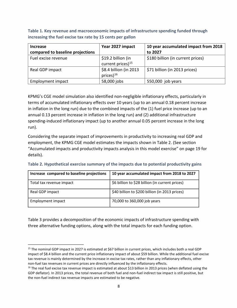
Table 1 provides key summary results of the model simulation on an increase in the fuel excise tax.

13 See http://www.kpmg-institutes.com/institutes/government-institute/articles/2017/03/funding-transportation-infrastructure-investment0.html. 14 The modeling simulation assumes no changes in the current vehicle technology, such as potential advances in electric or autonomous vehicles.

8

Table 1. Key revenue and macroeconomic impacts of infrastructure spending funded through increasing the fuel excise tax rate by 15 cents per gallon

Increase compared to baseline projections

Year 2027 impact 10 year accumulated impact from 2018 to 2027

Fuel excise revenue $19.2 billion (in current prices)15

$180 billion (in current prices)

Real GDP impact $8.4 billion (in 2013 prices)16

$71 billion (in 2013 prices)

Employment impact 58,000 jobs 550,000 job years

KPMG’s CGE model simulation also identified non-negligible inflationary effects, particularly in terms of accumulated inflationary effects over 10 years (up to an annual 0.18 percent increase in inflation in the long run) due to the combined impacts of the (1) fuel price increase (up to an annual 0.13 percent increase in inflation in the long run) and (2) additional infrastructure spending-induced inflationary impact (up to another annual 0.05 percent increase in the long run).

Considering the separate impact of improvements in productivity to increasing real GDP and employment, the KPMG CGE model estimates the impacts shown in Table 2. (See section “Accumulated impacts and productivity impacts analysis in this model exercise” on page 19 for details).

Table 2. Hypothetical exercise summary of the impacts due to potential productivity gains

Increase compared to baseline projections 10 year accumulated impact from 2018 to 2027

Total tax revenue impact $6 billion to $28 billion (in current prices)

Real GDP impact $40 billion to $200 billion (in 2013 prices)

Employment impact 70,000 to 360,000 job years

Table 3 provides a decomposition of the economic impacts of infrastructure spending with three alternative funding options, along with the total impacts for each funding option.

15 The nominal GDP impact in 2027 is estimated at $67 billion in current prices, which includes both a real GDP impact of $8.4 billion and the current price inflationary impact of about $59 billion. While the additional fuel excise tax revenue is mainly determined by the increase in excise tax rates, rather than any inflationary effects, other non-fuel tax revenues in current prices are directly influenced by the inflationary effects. 16 The real fuel excise tax revenue impact is estimated at about $13 billion in 2013 prices (when deflated using the GDP deflator). In 2013 prices, the total revenue of both fuel and non-fuel indirect tax impact is still positive, but the non-fuel indirect tax revenue impacts are estimated to be negative.

9

Note that by design all three funding options are modeled to raise the same level of revenue for additional infrastructure investment. All these three funding options are based on the principle of user pay funding. The maintenance costs of road infrastructure are closely linked to the level of use of vehicles and the weight of each vehicle, and the fuel excise tax is subject to ever-increasing fuel efficiency in the motor vehicle use. The VMT tax and the vehicle weight tax would be considered as new taxing options based on the more strictly defined user-pay principle.

Table 3. Comparison of long-run impacts of three user-pay principled funding options (Unit of measurement: Annual long run impacts deviation from baseline values)

Revenue Raised by Selected Tax Options/Infrastructure spending (billions in current prices)

Total Revenue Raised (billions in current prices)

Real GDP (billions in 2013 prices)

Real Private Consumption (billions in 2013 prices)

Employment (‘000 full time equivalents)

Infrastructure Spending only

$19.2 $30.8 $23.3 $18.5 111.0

Funding Option

Fuel Excise Tax only $19.2 $14.4 -$14.9 -$12.2 -53.4 VMT only $19.2 $15.9 -$11.1 -$8.6 -41.4

Weight Tax only $19.2 $13.3 -$15.3 -$9.4 -49.5 Total Impacts of Infrastructure Spending

with Fuel Excise Tax $19.2 $45.2 $8.4 $6.3 57.7 with VMT $19.2 $46.7 $12.2 $9.9 69.6

With Weight Tax $19.2 $44.1 $8.0 $9.1 60.5

The VMT tax option is expected to generate slightly higher impacts than the other two options. This indicates that the fuel excise tax option and the weight tax option are expected to result in more significantly adverse impacts on the business sector than the VMT option.

According to the current modeling analysis, the weight tax option has the lowest GDP impact. However with respect to the private consumption and the employment impacts, the fuel excise tax option is expected to have the lowest GDP impact. This indicates that household consumption is more sensitive to fuel prices and reflects the household sectors relatively large share of fuel consumption. At the same time, employment results turn out to be more sensitive to the fuel excise tax option, indicating the business cost impacts of an increase in the fuel excise tax are more negative than the other two tax options.

One of the conclusions derived from the economic impacts results reported in Table 6 is that adverse impacts from increases in tax revenue from the above selected tax funding options are fully offset by positive impacts of new additional infrastructure spending.

10

Fuel excise tax rate increases: Direct impact scenario The increased fuel excise tax rate used in the KPMG CGE modeling analysis is summarized along with the current fuel excise tax rates in Table 4. The federal excise tax rates under this scenario increase by a hypothetical 15 cents per gallon. It is also assumed in the modeling analysis that the additional tax revenue raised from the higher fuel excise tax rates is used to increase the allocation to the Mass Transit Account of the Highway Trust Fund beginning in 2018.

Table 4. Summary of the scenario of fuel excise tax rate increases (per gallon) Type of fuel Current excise tax rate Tax rate beginning in 2018 Gasoline* 18.4 cents 33.4 cents Diesel or Kerosene 24.4 cents 39.4 cents

Note: *Except for aviation gasoline.17 For the CGE modeling analysis, we assume in the base case that federal fuel excise tax rates will continue at their current levels.18 As a reference point, in fiscal year 2014, the federal fuel excise tax generated $25 billion in revenue, and the diesel fuel tax raised another $10.2 billion.19

Drivers of fuel tax revenue and assumptions for future fuel prices and volume

Setting aside the CGE analysis for a moment, federal fuel excise tax revenue in the coming years, generally depends on the following three factors:

1. Petroleum-related fuel prices, when indexed to inflation; 2. Petroleum-related fuel consumption by business and households; and 3. Excise tax rates.

Petroleum prices are heavily influenced by world market prices, and it is uncertain how long the recent relatively low petroleum prices in the world market may continue or how rapidly and to what levels petroleum prices may recover from current levels. Generally, forecasters believe that prices will increase gradually over the coming years, but not rise to the levels experienced in the early 2000’s.20

17 The current federal fuel excise for aviation gasoline is 19.4 cents per gallon. See the Internal Revenue Service Quarterly Federal Excise Tax Return (Form 720) for details. (www.irs.gov/pub/irs-pdf/f720.pdf) 18 The federal fuel excise tax was last raised in 1993 with no indexation to inflation. The current exemption from the tax for government entities is also assumed to continue in both the base case and the simulation using the higher fuel excise tax rates in Table 2. 19 For federal fuel excise tax revenue by calendar year, see (https://bea.gov/iTable/iTable.cfm?ReqID=9&step=1#reqid=9&step=3&isuri=1&903=90). 20 Based on the September 19, 2016 release of Long-Term Forecast Tables by Macroeconomic Advisers, (http://www.macroadvisers.com/) and KPMG analysis.

11

Considering the current over-capacity in the world gas market and developments in fuel reducing technology, future petroleum-related fuel consumption can only be projected with a significant amount of uncertainty and, therefore, a very wide range. The August 2016 annual energy outlook published by the U.S. Energy Information Administration (EIA)21 provides projections of U.S. crude oil production under five scenarios depending on the substitution possibilities with natural gas and the extent of new developments in technology. This implies that technology impacts in the natural gas industry as well as natural gas prices are important factors influencing the volume of crude oil demanded.

In the analysis of the potential impacts of an excise tax on gasoline under the CGE analysis, we use the following assumptions.

(1) Price projections in the base case: Gasoline prices recover to their 2006 levels in 2017, and reach their pre-2010 levels by 2020; after that, gasoline prices grow at a very moderate rate of 1.75 percent, per annum;22

(2) Volume projections in the base case reflect a scenario with a lower bound of consumption using the EIA forecasts,23 indicating marginal reductions in gasoline consumption over the first half of the 2020’s; and

(3) Federal fuel excise tax rates in the base case: Current federal gas excise tax rates, last increased in 1993, continue unchanged.

Tax revenue impacts As shown in Figure 1 below, KPMG’s CGE model simulation shows that the additional tax revenue from raising the federal fuel excise tax by 15 cents per gallon is projected to be $16.7 billion in 2018, reaching $18.4 billion by 2022 and $19.2 billion by 2027. As discussed in the box below, the additional fuel excise tax revenue of $19.2 billion24 in 2027 should be compared to

21 EIA, Annual Energy Outlook 2016 with projections to 2040, August 2016 (http://www.eia.gov/forecasts/aeo/). 22 Gasoline price projections come from Macroeconomic Advisors Long-Term Forecast of the U.S. Economy, released on September 19, 2016. A general description of the Microeconomic Advisors approach can be found at (http://www.macroadvisers.com/our-approach/). 23 See the scenario of “Low Oil and Gas Resource and Technology” in Figure ES-5, p. ES-4, EIA (2016) (https://www.eia.gov/forecasts/aeo/). 24 Under the baseline scenario where the current federal fuel excise rates remain unchanged without any inflation indexation, the projected fuel excise tax revenue in 2027 is roughly the same as the 2014 federal fuel excise tax revenue of $35.2 billion. Little growth of the projected federal fuel excise tax revenue over 13 years in the baseline scenario reflects the fact that projected volume in 2027 in the baseline is almost the same as the 2014 demand level. The additional federal fuel excise tax revenue of $19.2 billion is equivalent to a 60 percent increase compared to the projected baseline fuel excise tax revenue of $35 billion. Both the baseline federal fuel excise tax revenues and the additional fuel excise tax revenues are influenced by the low growth of fuel prices and demand projected in the baseline. The main reason for 60 percent growth of federal fuel excise tax revenue in 2027 which is lower than the 75 percent federal fuel excise rate increase that an additional 15 cents per gallon represents is due to demand contraction induced from the fuel price increases.

12

the nominal GDP impact of $67 billion in 2027 as the tax revenue impacts are measured in the current prices, i.e., nominal terms. Note that the nominal and real GDP impacts turn out to be vastly different due to accumulated inflationary effects over 10 years. See the box below for additional details.

General price impacts of this hypothetical exercise

The 15 cent per gallon increase in federal fuel excise tax rates used in KPMG’s CGE model simulation would lead to an about 3 percent increase in fuel prices if there were no behavioral responses in demand and supply (i.e., the so-called morning-after price impacts). Considering the private consumption share of fuel being about 2.5 percent, this would increase the consumer price index (CPI) by 0.075%.

Given the relatively low CPI impact when behavioral responses are not taken into account, the modeling results for CPI impacts, ranging from 0.18 percent (in the long run) to 0.35 percent (over the medium run), are considered to be significantly high. Such high inflationary outcomes are generated from the following two main factors.

(1) Relatively high use of fuel across the production sector as intermediate inputs would lead to cost-push inflationary effects on the economy-wide general price level.

(2) The additional infrastructure spending of about $19 billion would be equivalent to 1.7 percent of the output of the entire construction industry. Because the construction industry is relatively labor intensive, there would be additional wage income, which would lead to demand induced inflationary effects across all products consumed by the household sector.

The relatively large price effect makes the nominal GDP effect much larger than the real GDP effect in terms of both the growth and level-form impact.

Such relatively high inflationary effects will be smaller or neutralized if productivity gains are introduced. This is because in a competitive market, any productivity gains will eventually be reflected in lower prices.

The CGE model’s relatively slow growth of projected revenue from 2022 through 2027 reflects the assumed stabilization of expected fuel prices in 2022 after a relatively strong recovery of projected fuel prices beginning in 2017. Overall, the projected fuel excise tax revenue growth is driven by the slow growth of the consumed value of gasoline and diesel fuel in current prices, which in turn reflects the assumed projections of a moderate growth in fuel prices and a slight decrease in fuel volume consumed from 2018 forward. Note that the fuel tax rates used in the simulation are indexed to fuel price inflation in the modeling analysis. Therefore, these estimated tax revenues are generated from a very conservative scenario regarding future gasoline prices and future demand in the baseline scenario.

Figure 1 shows the additional federal fuel excise tax revenue from 2018 to 2027.

13

If the world oil market performs better and the anticipated excess capacity in the world gas market is not realized as expected, then the above revenue estimates could be significantly understated. The opposite would result if the market does not perform as expected or the excess capacity assumed in the simulation is not realized. KPMG’s CGE modeling is based on the best available information at the time a simulation was performed. As events change or as better information becomes available, it is important to re-run the model.

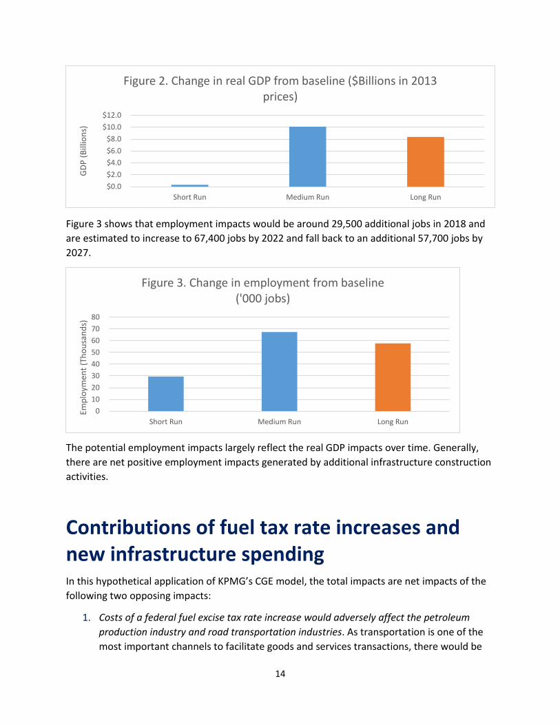
Real GDP and employment impacts In terms of potential real GDP impacts (in 2013 prices25), net of productivity gains,26 Figure 2 shows the net gain in 2018 would be about $0.3 billion.27 Annual real GDP benefits would increase up to $10.1 billion in 2022, and after that long-term annual net gains become smaller, reaching $8.4 billion in 2027.28

25 The base year in the CGE model database is calibrated to the U.S. economy using the BEA 2013 input-output tables. This was the most recent information at the time the development of the core CGE database in 2015. As stated in footnote 7, periodically, using new BEA information, KPMG’s CGE would be updated to ensure its continued relevance as a modeling tool. 26 The economic impacts discussed in this section are the impacts of the federal fuel excise tax increases and additional construction activities for new or upgraded road infrastructure. The modeling results in Figure 2 do not take into account any productivity gains which could be generated from operating new infrastructure. The productivity impacts are separately estimated and discussed later in this research paper. 27 The negligible GDP impact in 2018 reflects only partial adjustments in capital stock at the industry level in response to new infrastructure and tax changes. Wage rigidity in the labor market limits the full adjustment of the economy in the short run. Therefore, the first year’s impact takes into account the adjustment costs of the economy in response to the increases in the federal fuel excise tax rate. 28 Due to the long-term constraint on the external balance of the U.S. economy, there would be offsetting impacts from adjusted saving behavior. Such long-term offsetting impacts make the long-run GDP impact smaller than the medium-run impact.

15

16

17

18

19

20

2018 2019 2020 2021 2022 2023 2024 2025 2026 2027

Figure 1. Additional federal fuel excise revenue ($Billions in current prices)

14

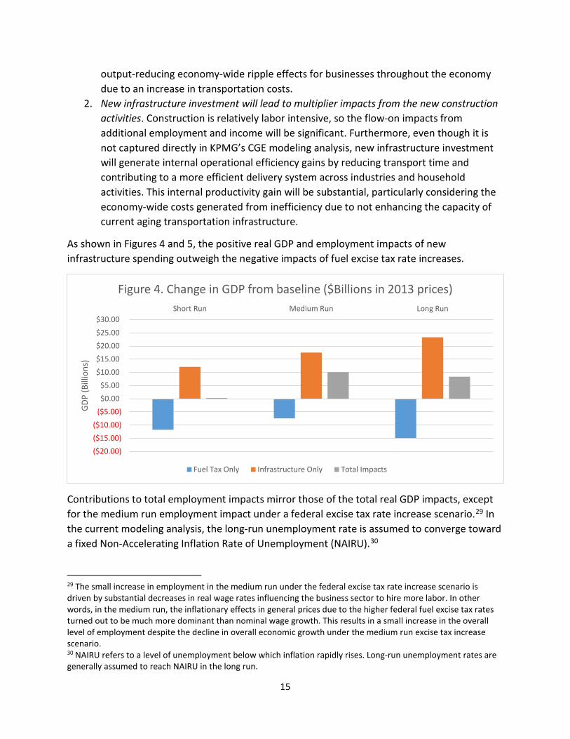
Figure 3 shows that employment impacts would be around 29,500 additional jobs in 2018 and are estimated to increase to 67,400 jobs by 2022 and fall back to an additional 57,700 jobs by 2027.

The potential employment impacts largely reflect the real GDP impacts over time. Generally, there are net positive employment impacts generated by additional infrastructure construction activities.

Contributions of fuel tax rate increases and new infrastructure spending In this hypothetical application of KPMG’s CGE model, the total impacts are net impacts of the following two opposing impacts:

1. Costs of a federal fuel excise tax rate increase would adversely affect the petroleum production industry and road transportation industries. As transportation is one of the most important channels to facilitate goods and services transactions, there would be

$0.0$2.0$4.0$6.0$8.0

$10.0$12.0

Short Run Medium Run Long Run

GDP

(Bill

ions

)Figure 2. Change in real GDP from baseline ($Billions in 2013

prices)

01020304050607080

Short Run Medium Run Long Run

Empl

oym

ent (

Thou

sand

s)

Figure 3. Change in employment from baseline ('000 jobs)

15

output-reducing economy-wide ripple effects for businesses throughout the economy due to an increase in transportation costs.

2. New infrastructure investment will lead to multiplier impacts from the new construction activities. Construction is relatively labor intensive, so the flow-on impacts from additional employment and income will be significant. Furthermore, even though it is not captured directly in KPMG’s CGE modeling analysis, new infrastructure investment will generate internal operational efficiency gains by reducing transport time and contributing to a more efficient delivery system across industries and household activities. This internal productivity gain will be substantial, particularly considering the economy-wide costs generated from inefficiency due to not enhancing the capacity of current aging transportation infrastructure.

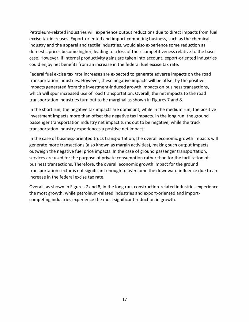
As shown in Figures 4 and 5, the positive real GDP and employment impacts of new infrastructure spending outweigh the negative impacts of fuel excise tax rate increases.

Contributions to total employment impacts mirror those of the total real GDP impacts, except for the medium run employment impact under a federal excise tax rate increase scenario.29 In the current modeling analysis, the long-run unemployment rate is assumed to converge toward a fixed Non-Accelerating Inflation Rate of Unemployment (NAIRU).30

29 The small increase in employment in the medium run under the federal excise tax rate increase scenario is driven by substantial decreases in real wage rates influencing the business sector to hire more labor. In other words, in the medium run, the inflationary effects in general prices due to the higher federal fuel excise tax rates turned out to be much more dominant than nominal wage growth. This results in a small increase in the overall level of employment despite the decline in overall economic growth under the medium run excise tax increase scenario. 30 NAIRU refers to a level of unemployment below which inflation rapidly rises. Long-run unemployment rates are generally assumed to reach NAIRU in the long run.

($20.00)($15.00)($10.00)

($5.00)$0.00$5.00

$10.00$15.00$20.00$25.00$30.00

Short Run Medium Run Long Run

GDP

(Bill

ions

)

Figure 4. Change in GDP from baseline ($Billions in 2013 prices)

Fuel Tax Only Infrastructure Only Total Impacts

16

Over the medium and long run, as shown in Figure 6, household consumption impacts turn out to be positive as the adverse impacts of higher fuel prices would be more than offset by positive construction induced employment impacts. However, in the short run, negative impacts from higher fuel prices are not fully offset by positive investment impacts because new investment induced employment impacts are not yet fully realized due to constraints on full capital stock adjustments by industry in the short run.

Industry impacts in this model exercise The industry impacts are not uniform. Due to infrastructure investment, the construction industry and those industries supplying inputs to the construction industry, such as the non-metallic mineral industry, wood products industry and general retail industry, will realize greater than average benefits from an increase in the federal fuel excise tax rate and increased spending on transportation infrastructure.

(300)

(200)

(100)

0

100

200

300

Short Run Medium Run Long Run

Empl

oym

ent (

Thou

sand

s)Figure 5. Change in employment from baseline ('000 jobs)

Fuel Tax Only Infrastructure Only Total Impacts

($10.00)

$0.00

$10.00

$20.00

$30.00

Short Run Medium Run Long Run

Impo

rts (

Billi

ons)

Figure 6. Change in private consumption($Billions in 2013 prices)

17

Petroleum-related industries will experience output reductions due to direct impacts from fuel excise tax increases. Export-oriented and import-competing business, such as the chemical industry and the apparel and textile industries, would also experience some reduction as domestic prices become higher, leading to a loss of their competitiveness relative to the base case. However, if internal productivity gains are taken into account, export-oriented industries could enjoy net benefits from an increase in the federal fuel excise tax rate.

Federal fuel excise tax rate increases are expected to generate adverse impacts on the road transportation industries. However, these negative impacts will be offset by the positive impacts generated from the investment-induced growth impacts on business transactions, which will spur increased use of road transportation. Overall, the net impacts to the road transportation industries turn out to be marginal as shown in Figures 7 and 8.

In the short run, the negative tax impacts are dominant, while in the medium run, the positive investment impacts more than offset the negative tax impacts. In the long run, the ground passenger transportation industry net impact turns out to be negative, while the truck transportation industry experiences a positive net impact.

In the case of business-oriented truck transportation, the overall economic growth impacts will generate more transactions (also known as margin activities), making such output impacts outweigh the negative fuel price impacts. In the case of ground passenger transportation, services are used for the purpose of private consumption rather than for the facilitation of business transactions. Therefore, the overall economic growth impact for the ground transportation sector is not significant enough to overcome the downward influence due to an increase in the federal excise tax rate.

Overall, as shown in Figures 7 and 8, in the long run, construction-related industries experience the most growth, while petroleum-related industries and export-oriented and import-competing industries experience the most significant reduction in growth.

18

-1.5-1

-0.50

0.51

1.5

Figure 7. Selected industry GDP impacts (%)

Short run Medium Run Long Run

-1.5

-1

-0.5

0

0.5

1

Figure 8. Selected industry employment impacts (%)

Short run Medium Run Long Run

19

Accumulated impacts and productivity impacts in this model exercise The economic impact results presented so far have not included any consideration of potential productivity impacts. However, in policy modeling discussions, economic impacts are often discussed in terms of accumulated impacts over time, typically over a 10-year period. In the current scenario, federal fuel excise tax rates are assumed to increase permanently and all of the increase in fuel excise tax revenues are also assumed to be allocated each year to the Highway Trust Fund for additional construction of road transportation infrastructure. From this point of view, in this section, the first 10 years accumulated impacts without any consideration of productivity impacts are reported along with a separate analysis of the potential accumulated productivity impacts.

The internal productivity or any operational efficiency gains of new infrastructure investment are expected to generate more lasting impacts than its construction impacts.31 However, it is difficult to measure such productivity gains using observable indicators at an aggregate level of the economy. To avoid such speculative impacts, we present the results without any productivity gains and will separately state the results including a range of possible productivity gains.

Potential productivity improvement

In 2012, the Department of the Treasury and the Council of Economic Advisers32 discussed the potential costs of congestion and the additional investment required to repair the existing road transportation infrastructure. In doing so, they relied on the following two research studies. The first study is covered in the 2013 DOT report earlier cited where DOT estimated that $85 billion in total investment per year over the next 20 years (i.e., a total cost of $1.7 trillion) would be required to bring existing highways and bridges into a state of good repair. 33

The second study is the 2015 Urban Mobility Scorecard,34 which found that in 2014, congestion caused commuters in 471 urban areas to travel an extra 6.9 billion hours and purchase an extra 3.1 billion gallons of fuel for a congestion cost of $160 billion. The average yearly delay per urban commuter was 42 hours – more than a full work week. Commuters in cities such as

31 While the construction impacts are limited over the construction period only, the operational impacts of new infrastructure would last over the life time of the new infrastructure. 32 The Department of the Treasury with the Council of Economic Advisers, “A New Economic Analysis of Infrastructure Investment,” March 23, 2012 (https://www.treasury.gov/resource-center/economic-policy/Documents/20120323InfrastructureReport.pdf). 33 See footnote 1. 34 “2015 Urban Mobility Scorecard,” August 2015, jointly published by the Texas A&M Transportation Institute (mobility.tamu.edu) and INRIX, Inc. (inrix.com) (http://d2dtl5nnlpfr0r.cloudfront.net/tti.tamu.edu/documents/mobility-scorecard-2015.pdf).

20

Washington, DC, which led the list at 82 hours of delay per commuter, experienced even higher delay times.

Some economists have published estimates of the productivity impacts due to insufficient infrastructure investment. For example, in 2016, ASCE estimated that the $160 billion congestion cost translated to an increase of 91 cents per gallon in the federal fuel excise tax rate. 35

If it is assumed that the annual congestion-oriented inefficiency cost of $160 billion per annum could be fully addressed when the aforementioned required investment cost of $1.7 trillion is fully met, an annual productivity gain per billion dollars of infrastructure spending is benchmarked as $94 million, or 9.4 percent.

This benchmarked productivity gain is estimated on the basis of the following additional assumptions: (1) the infrastructure spending is entirely used for fix-it-first investments and (2) all of the above congestion cost is due to the lack of road repair. Since congestion can be caused by other than the lack of road repair, we set up a potential lower and upper bound for the potential productivity gains due to additional infrastructure spending.

For our model exercise, we assume that 20 percent to 80 percent of the abovementioned congestion cost could be resolved by new infrastructure spending. Given the uncertainty of the efficiency impacts of new infrastructure spending, a wide range of potential efficiency impacts was selected to highlight the nature of uncertainty in relation to the efficiency impacts. Based on the ASCE estimate of 91 cents per gallon of federal fuel excise rate increase,36 we have equated the potential efficiency saving to roughly between 20 cents and 75 cents per gallon.

The simulation uses this 20 percent to 80 percent range of congestion costs to develop an estimate of the range of productivity gains which can be achieved with additional infrastructure spending.

Accumulated tax revenue impact (net of productivity impacts)

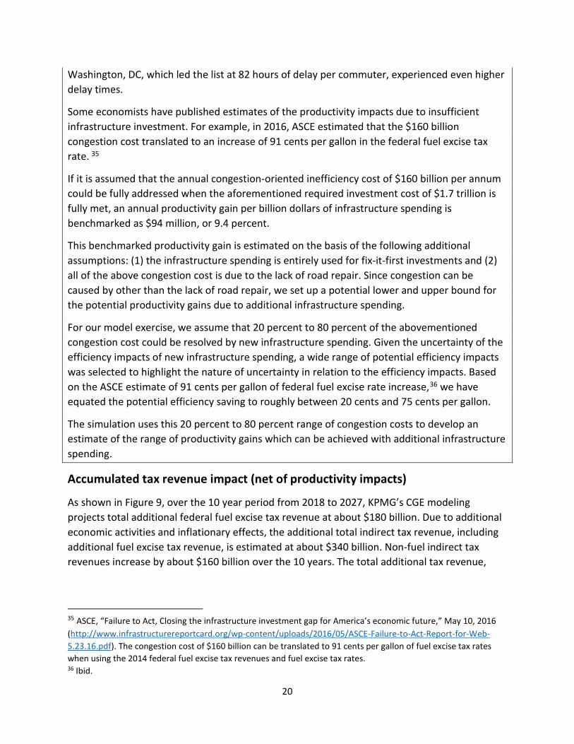
As shown in Figure 9, over the 10 year period from 2018 to 2027, KPMG’s CGE modeling projects total additional federal fuel excise tax revenue at about $180 billion. Due to additional economic activities and inflationary effects, the additional total indirect tax revenue, including additional fuel excise tax revenue, is estimated at about $340 billion. Non-fuel indirect tax revenues increase by about $160 billion over the 10 years. The total additional tax revenue,

35 ASCE, “Failure to Act, Closing the infrastructure investment gap for America’s economic future,” May 10, 2016 (http://www.infrastructurereportcard.org/wp-content/uploads/2016/05/ASCE-Failure-to-Act-Report-for-Web-5.23.16.pdf). The congestion cost of $160 billion can be translated to 91 cents per gallon of fuel excise tax rates when using the 2014 federal fuel excise tax revenues and fuel excise tax rates. 36 Ibid.

21

including all direct and indirect taxes is $510 billion over the 10 years, indicating an additional $170 billion is attributable to individual and corporate income tax revenues.

The above total additional tax revenues include the inflationary impacts on the overall economy. Therefore, it is also important to assess the real impacts on the US economy of raising the federal fuel excise tax rate.

Additional tax revenue impacts due to productivity impacts

Figure 10 shows the accumulated tax revenue impacts under productivity improvement scenarios as discussed above. There are only marginal impacts on fuel excise tax revenues due to productivity gains. Accumulated additional fuel excise tax revenues due to productivity gains are estimated at a range of $24 million to $117 million depending on the assumption for the benefit attributable to improvements in productivity.

The accumulated total indirect tax revenue increases by $1.1 billion and $5.3 billion under each of the lower and upper-bound scenario. These productivity contributions are small compared to the accumulated total indirect tax revenue impact of $340 billion due to the infrastructure spending funded by the federal fuel excise tax rate increase as shown earlier in Figure 9.

The accumulated total direct tax contributions are projected to be larger than the accumulated total indirect tax contributions from improvements to productivity as the accumulated total tax revenue increases by $6 billion to $28 billon depending on the assumption of benefit attributable to improvements in productivity.

$0.0

$100.0

$200.0

$300.0

$400.0

$500.0

$600.0

Fuel Excise Revenue Total Indirect Tax Revenue Total Tax Revenue

Tax

Reve

nue

(Bill

ions

)

Figure 9. Gross tax revenues over 10 years: 2018-2027 ($Billions in current prices)

22

Accumulated and productivity impacts on real GDP

As shown in Figure 11, the accumulated total real GDP impact over 10 years from 2018 to 2027, under this hypothetical analysis, is estimated at about $71 billion in 2013 prices and the accumulated total additional productivity gains are estimated at between $40 billion and $200 billion over the 10 years. Under the lower-bound assumption for productivity improvement, the accumulated additional productivity impact is more than 50 percent of the accumulated impact due to the scenario for new infrastructure spending funded by federal fuel excise tax rate increases, which excludes any productivity gains. Using the upper-bound assumption for productivity improvement, the real GDP impacts are almost three times larger than the real GDP impact under the scenario for new infrastructure spending funded by federal fuel excise tax rate increases. This implies that the productivity impacts can be much larger than the construction impacts, particularly in the long run. This is because productivity impacts are by nature cumulative; i.e., getting larger compared to the baseline as new infrastructure is continuously expanding over the projected period of 10 years.

$0.0

$5.0

$10.0

$15.0

$20.0

$25.0

$30.0

Fuel Excise Revenue Total Indirect Tax Revenue Total Tax Revenue

Figure 10. Gross tax revenues over 10 years: 2018-2027 from productivity gains

($Billions in current prices)

Additional Productivity Gains_Lower Additional Productivity Gains_Upper

23

Accumulated and productivity impacts on employment

The accumulated employment impact over 10 years from 2018 to 2027 is estimated at about 550,000 job years.

The accumulated total employment impacts due to productivity improvement over 10 years from 2018 to 2027 are estimated at between 74,000 and 360,000 job years as shown in Figure 12. When compared to the real GDP impact, the accumulated employment impact over 10 years from additional productivity improvements is relatively small. Observing that the productivity effect on real GDP is greater than the productivity effect on employment, we can infer that capital intensive industries, such as heavy manufacturing industries, generally benefit more than labor intensive industries from the productivity improvements.

$0.0

$50.0

$100.0

$150.0

$200.0

Real GDP Additional Productivity Gains_Lower Additional Productivity Gains_Upper

Figure 11. Gross real GDP impacts over 10 years: 2018-2027 ($Billions in 2013 prices)

-

100.0

200.0

300.0

400.0

500.0

600.0

Employment Additional Productivity Gains_Lower Additional Productivity Gains_Upper

Figure 12. Gross employment impacts over 10 years: 2018-2027 ('000 job years)

24

Additional long-run industry impacts of productivity gains

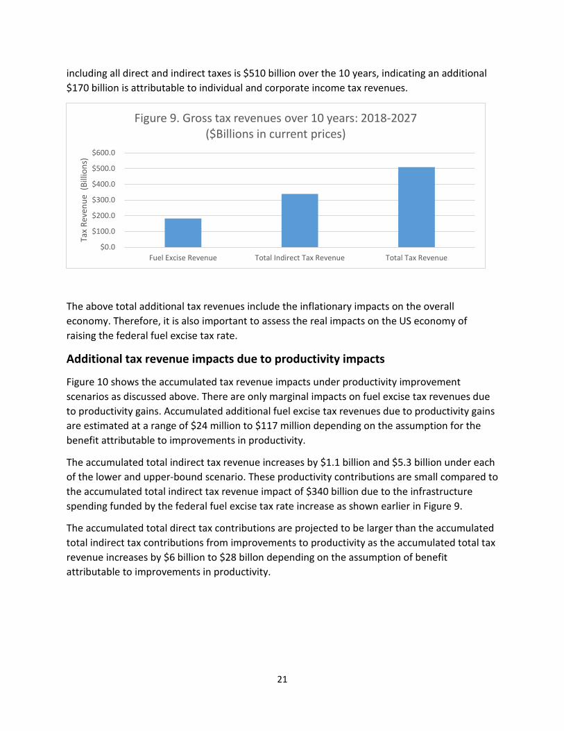
Figures 13 and 14 show selective industry impacts from long-run productivity gains.

The primary metal products industry shows the largest long-run productivity gains for both industry GDP and employment in terms of the percentage deviation from the baseline.37

Figures 13 and 14 show the productivity gains spread across the mining, utility, manufacturing, retail, and services sectors. Some private consumption-oriented industries with relatively lower use of road transport services, such as the apparel industry, would suffer the most as their relative price disadvantages from an international competitiveness point of view would lead to a significant reduction in their demand.

The very high gains observed in the primary metal products industry in the productivity impact analysis are driven largely by the combined effects of the following two factors: (1) a high level use of road transportation services in its production and delivery and (2) a high level of export growth and import substitution effects38 of the primary metal products industry in response to its productivity induced price changes.

Some industries using relatively lower road transport services, such as government enterprise industries and the waste management industry, do not share the overall economy-wide benefits due to expected productivity gains.

Overall, the operational productivity gains are considered to be substantially large and the industry distributions of the productivity gains are quite different from the federal fuel excise tax funded infrastructure construction impacts. Furthermore, the productivity gains are more uniformly spread across the production sector compared to the infrastructure construction gains.

37 The road transportation industry output also grows at rates similar to the rate of the primary metal products industry. However, its employment levels are lower than the baseline employment as the road transportation industry can generate the same level of outputs using fewer employees. 38 The import substitution elasticities in the model are calibrated at 4.0 to reflect high levels of import competition and price sensitivity in determining the supply sources.

25

-0.05 0 0.05 0.1 0.15 0.2 0.25

Primary Metal ProductsOther Mining

Water TransportUtilities

Motor Vehicle RetailFurniture

Electrical EquipmentNon Metallic Mineral Prodcuts

Food Beverage TobaccoRecreation Servicces

Housing & Real EstateFunds & Trusts

EducationApparel

Figure 13. Long-run productivity gains:Selective industry GDP Impacts (%)

-0.05 0 0.05 0.1 0.15 0.2 0.25

Primary Metal ProductsOther Mining

Water TransportUtilities

Motor Vehicle RetailFurniture

Electrical EquipmentNon Metallic Mineral Prodcuts

Food Beverage TobaccoRecreation Servicces

Housing & Real EstateFunds & Trusts

EducationApparel

Figure 14. Long-run productivity gains:Selective industry employment impacts (%)

26

Price elasticity analysis To assess the sensitivity of the CGE model results of the calibrated values related to fuel price elasticity, the following sensitivity tests are conducted. The currently calibrated value of the fuel price elasticity in the CGE model is in line with the average -0.6 estimate of the long-run price elasticity for developed countries.39 U.S. short-run elasticity ranges from -0.21 to -0.34,40 which is comparable with the average estimate of the short-run elasticity of -0.26 for developed countries.41 These short-run estimates became much smaller during the more recent period.42

For the sensitivity analysis, KPMG’s CGE model used two alternative values to compare to the average calibrated price elasticity of -0.6. They are: (1) Upper value: -1.0 and (2) Lower value: -0.3. The lower value reflects the average estimate of short-run price elasticities.43 The upper value represents the maximum possible value for the good, which is considered to be inelastic to price changes. This is because fuel in the U.S. is considered to be price inelastic, particularly over the recent time period.44 Furthermore, fuel for private consumption is considered to be a necessary product rather than a luxury good in the U.S. Therefore, fuel price elasticity higher than -1 (in absolute terms) may not be plausible for the U.S. economy.

The sensitivity results, using the upper and lower elasticity range above in the long run, are summarized in Table 5:

Table 5. Sensitivity test results of the long-run analysis using alternative estimates of fuel price elasticity

Fuel price elasticity Current (-0.6) Upper (-1.0) Lower (-0.3)

Fuel excise revenue (current prices)

$19.2 Billion $17.6 Billion $19.7 Billion

Real GDP (in 2013 prices) $8.4 Billion $6.0 Billion $12.1 Billion

Employment 58,000 57,000 68,000

Under the upper price elasticity scenario, the tax revenue gain decreases by 8.5 percent from $19.2 to $17.6 billion and the real GDP impact decreases by 28 percent from $8.4 billion to $6.0

39 “Gasoline demand revisited: an international meta-analysis of elasticities,” by Molly Espey, “Energy Economics 20,” pages 273 to 295, February 1998. (https://www.researchgate.net/publication/4944089_Gasoline_demand_revisited_an_international_meta-analysis_of_elasticities). 40“Evidence of a Shift in the Short-run Price Elasticity of Gasoline Demand,” by Jonathan E. Hughes, Christopher R. Knittel and Daniel Sperling, The Energy Journal, Vol. 29, No. 1, pages 93 to 124, 2008 (http://web.mit.edu/knittel/www/papers/gas_demand_final.pdf). 41 See footnote 34. 42 See footnote 39. 43 See footnotes 38 and 39. 44 ibid.

27

billion. The employment impact under the upper price elasticity scenario is small as it decreases by only 1.5 percent or 1,000 jobs. This indicates that the employment impacts are influenced more by additional infrastructure spending than by fuel excise tax rate increases.

Under the lower price elasticity scenario, the tax revenue gain increases by 2.6 percent to $19.7 billion, and the real GDP impact increases by about 44 percent to $12.1 billion. The employment impact under the lower price elasticity scenario is moderate as it increases by 17 percent or 10,000 jobs. This indicates that the adverse effect on employment is smaller than the adverse effect on real GDP in the fuel industry because it is a more capital intensive industry and there is a labor supply constraint in the long run.

Overall, the economy-wide impacts are quite sensitive to the choice of the implicit fuel price elasticity value. The lower the fuel price elasticity, the larger the economy-wide positive impacts. Nevertheless, the additional federal fuel excise tax revenue results are not particularly sensitive to the choice of the fuel price elasticity value. This indicates that the indirect and induced impacts of the fuel price increases are much more important than direct impacts of the fuel excise tax rate increases.

Furthermore, the net positive outcome of the increased federal fuel excise tax funded infrastructure spending are considered to be robust, despite the fact that the magnitude of net positive benefits tends to vary according to the calibrated value of the fuel price elasticity. Especially when considering the very low short-run price elasticities, estimated to range from -0.034 to -0.077 over the period from 2001 to 200645 (relative to the price elasticity used in the current modeling analysis which ranges from -0.03 to -1.0), the current CGE modeling results of the macroeconomic impacts are considered to be very conservative.

45 See footnotes 38 and 39.

28

Potential Vehicle mileage traveled tax and motor vehicle weight tax: Direct impact scenarios

As highlighted earlier, the current federal fuel excise tax, which is a main funding source of the nation’s highways, is not sufficient to cover ever-increasing funding requirements. Furthermore, fuel excise tax revenue over the coming years is not expected to rise due to increasingly more fuel-efficient vehicles and increased use of electric vehicles even at a small scale. From this perspective, alternative funding options in addition to the federal fuel use tax have been discussed. For example, a CBO report provides qualitative discussions about pros and cons of the fuel excise tax and a VMT. 46 Another CBO paper discusses alternative tax options for freight transportation (truck and rail) to recover external costs.47 The policy options discussed in that CBO paper include a shipment weight tax, distance tax, fuel use tax, container tax, truck tire tax, and a combination of these options. A range of non-tax options are discussed in a publication of the Global Economic Governance Initiative at Boston University.48

Based on a review of this literature, two options in addition to the raising the fuel excise tax rate were selected for the CGE modeling analysis included in this economic research modeling paper. This section discusses how to model the VMT tax and motor vehicle weight tax (referred to as weight tax hereafter) for the CGE model simulations. All revenue raised by these alternative tax options, as well as increasing in the fuel excise tax, are assumed to be used for additional infrastructure spending. Therefore, to make proper comparisons of these three potential funding options in terms of the economy-wide flow-on impacts, the rates of the VMT and weight tax are calibrated to raise revenue equivalent to that raised by the federal fuel excise tax rate increase previously modeled.

VMT tax: Direct Impact Scenario

As reported in Table 1, the additional annual tax revenue from raising the federal fuel excise tax by 15 cents per gallon is projected to reach $19.2 billion by 2027.

46 Congressional Budget Office (CBO), “Alternative Approaches to Funding Highways”, CBO report, March 2011 (https://www.cbo.gov/publication/22059?index=12101). 47 “Pricing Freight Transport to Account for External Costs,” by David Austin Congressional Budget Office, Working Paper 2015-03, March 30, 2015 (https://www.cbo.gov/publication/50049). 48 “Financing Sustainable Infrastructure in the Americas,” by Rogério Studart and Luma Ramos, Global Economic Governance Initiative, Boston University, GEGI working paper 007, July 2016 (http://www.bu.edu/pardeeschool/files/2016/08/Financing-Sustainable.-StudartRamos.pdf).

29

According to the Department of Transportation and an automotive market research agency, in 2013, about 250,000 registered vehicles traveled a total of 3,369 billion miles.49 These statistics imply that on average vehicles traveled about 13,500 miles in 2013. Without consideration of any behavioral impacts due to a VMT tax, the required VMT tax rate to raise $19.2 billion is 0.57 cents per mile, which equates to $77 per vehicle on average for the year 2013.

Once a VMT is introduced, there would be a reduction in vehicle use through a reduction in vehicles and/or reduced miles driven per vehicle. According to KPMG’s CGE modeling analysis, to raise $19.2 billion in the long run, the required VMT tax rate is estimated at 0.74 cents per mile.

For this direct impact estimation of a VMT tax, a single VMT tax rate is assumed to be applied to all types of vehicle travel. However, VMT rates can be different according to the vehicle type, the time of travel and the road type of vehicle travel.50 In this case, the administration and compliance costs can be high, and there could also be a privacy protection issue. While a more complicated VMT tax can be modeled, for demonstration purposes, a simple single rate of a VMT tax is assumed for the current study.

Weight tax: Direct impact scenario

CBO reported that, on average, the estimated cost of pavement damage caused by a truck is almost 77 times higher than a passenger vehicle.51 It also reported that the total mileage share of trucks is about 10 percent versus 90 percent for passenger vehicles.

Using this information along with the transportation industry output data recorded in the KPMG’s CGE database,52 the ratio of an average weight tax per dollar for the truck industry to the average weight tax per dollar for the passenger vehicle industries is estimated at 12.7. This implicit ratio is used to calibrate the weight tax rate per dollar for the truck and ground passenger industry outputs to achieve additional revenue of $19.2 billion. After taking into account all behavioral responses of economic agents, KPMG’s CGE modeling results indicate the required weight tax rates in the long run are 6.5 cents per $1 worth of truck transport industry output and 0.5 cent per $1 worth of ground passenger transport industry output.

For the weight tax option, impacts on weight tax revenues due to the behavioral responses are expected to be much higher than the VMT tax option. For the VMT tax option, the increase in

49 U.S. Department of Transportation Federal Highway Administration, “State Motor-Vehicle Registrations – 2010 table 1” (https://www.fhwa.dot.gov/policyinformation/statistics/2010/pdf/mv1.pdf and https://hedgescompany.com/automotive-market-research-statistics/auto-mailing-lists-and-marketing). 50 See footnote 46.

51 ibid 52 Note that there are three road transportation industries in the KPMG’s CGE model – ground passenger transport, truck transport and other transport including sightseeing and supports. The passenger vehicle industry is assumed to include ground passenger transport, a portion of other transport, and household ownership of motor vehicles.

30

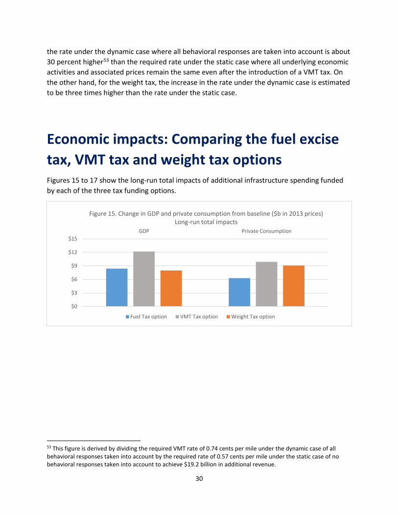
the rate under the dynamic case where all behavioral responses are taken into account is about 30 percent higher53 than the required rate under the static case where all underlying economic activities and associated prices remain the same even after the introduction of a VMT tax. On the other hand, for the weight tax, the increase in the rate under the dynamic case is estimated to be three times higher than the rate under the static case.

Economic impacts: Comparing the fuel excise tax, VMT tax and weight tax options Figures 15 to 17 show the long-run total impacts of additional infrastructure spending funded by each of the three tax funding options.

53 This figure is derived by dividing the required VMT rate of 0.74 cents per mile under the dynamic case of all behavioral responses taken into account by the required rate of 0.57 cents per mile under the static case of no behavioral responses taken into account to achieve $19.2 billion in additional revenue.

$0

$3

$6

$9

$12

$15GDP Private Consumption

Figure 15. Change in GDP and private consumption from baseline ($b in 2013 prices)Long-run total impacts

Fuel Tax option VMT Tax option Weight Tax option

31

According to the current modeling analysis, the weight tax option is considered to have the least long-run impact on GDP. However in terms of the private consumption and employment impacts, the fuel excise tax option is expected to have the least impact. This indicates that household consumption is sensitive to fuel prices, reflecting that the household sector uses a relatively large share of fuel consumption. At the same time, employment results turn out to be more sensitive to the fuel excise tax option, indicating that business cost impacts of an increase in the fuel excise tax are more severe than the other two tax options.54

54 Note that all the tax rates of the selected tax options are assumed to be inflation indexed. Therefore, the calibration of each tax rate in the current analysis is closely related to the price forecasts of the relevant goods in the long run. In the current analysis, the fuel price inflation is assumed to be lower than consumer price inflation at least for the next decade. If the fuel price inflation is assumed to be similar to consumer price inflation, the economic impacts of the fuel excise tax option are expected to be better than the current modeling results. This is because the increase in the fuel excise tax rate required to meet the target revenue for additional infrastructure spending would be lower if the fuel price inflation is assumed to be higher than the current case.

0

20

40

60

80

Fuel Tax Option VMT Tax option Weight Tax OptionEmpl

oym

ent (

Thou

sand

s)Figure 16. Change in employment from baseline - Total long-run impacts

('000 persons)

$0.0

$10.0

$20.0

$30.0

$40.0

$50.0

Fuel Tax Option VMT Tax option Weight Tax OptionTax

Reve

nue

(Bill

ions

)

Figure 17. Gross tax revenues - Total long-run Impacts($b in current prices)

32

Table 6 (which repeats what is in Table 3) provides a decomposition of the economic impacts of infrastructure spending with three alternative funding options along with the total impacts with each funding option. Note that the all three funding options are modeled to raise the same level of revenue to use for additional infrastructure investment.

Table 6. Comparison of long-run impacts of these three user-pay principled funding 0ptions55 (unit: annual long run impacts deviated from the baseline values)

Revenue Raised by Selected Tax Options/Infrastructure spending(ii) (billions in current prices)

Total Revenue Raised (billions in current prices)

Real GDP (billions in 2013 prices)

Real Private Consumption (billions in 2013 prices)

Employment (‘000 full time equivalents)

Infrastructure Spending only(i)

$19.2 $30.8 $23.3 $18.5 111.0

Funding Option

Fuel Excise Tax only $19.2 $14.4 -$14.9 -$12.2 -53.4 VMT only $19.2 $15.9 -$11.1 -$8.6 -41.4

Weight Tax only $19.2 $13.3 -$15.3 -$9.4 -49.5 Total Impacts of Infrastructure Spending

with Fuel Excise Tax $19.2 $45.2 $8.4 $6.3 57.7 with VMT $19.2 $46.7 $12.2 $9.9 69.6

With Weight Tax $19.2 $44.1 $8.0 $9.1 60.5 (i) Most of interactive impacts of the infrastructure spending along with each tax option are

allocated to infrastructure spending only scenario. (ii) The figures are target values of each simulation, however, the actual results are more or less

close to the target values.

The VMT tax option is considered to generate slightly higher macroeconomic impacts than the other two options. This indicates the fuel excise tax option and the weight tax option are expected to result in more severe adverse effects on the business sector than the VMT tax option.

55 The current approach can be considered as eclectic as the comparative static or snapshot analysis are applied to trend forecasts of the relevant variables, which are independently derived from the CGE modeling. Therefore, all the figures in the table should be considered to be indicative. When specific price forecasts are important in the evaluation of potential tax revenue and other macroeconomic impacts, the year-by-year comparative dynamic analysis would provide more accurate assessments of potential revenue impacts. Nevertheless, when the results from the current eclectic approach are compared to those from the year-by-year comparative dynamic modeling analysis, the three snap shot based eclectic approach adopted in the current paper can be considered to be a reasonable representation of the year-by-year comparative dynamic modeling analysis.

33

One of the conclusions derived from the economic impact results reported in Table 6 is that adverse impacts from increases in tax revenue from the above selected tax funding options are fully offset by positive impacts of new additional infrastructure spending. In addition, the transit and ground passenger transportation industry and truck transportation industry have significantly different impacts under the three tax funding options in terms of the proportional change impacts deviated from the baseline. For example, the impacts on the truck transportation industry are the greatest under the weight tax option.

Again, it is important to emphasize that the above comparisons should not be interpreted as any preference of any specific tax funding option against another or even the adoption of a VMT tax or a weight tax. As mentioned in the introduction, there are many other important criteria for the evaluation of tax options, including equity issues, compliance and administration issues, and tax revenue raising capacity. Therefore, the above comparisons should be considered as part of the demonstration purpose of KPMG’s CGE modeling capacity.

Conclusion

Public policy decision-makers will need quality information to help consider the range of financing options and potential impacts on the economy and the public, both positive and negative, from infrastructure investment. As demonstrated in this research paper, KPMG’s CGE model is an effective tool to assess policy options in terms of impacts on revenue, real GDP, employment, productivity, and various U.S. industries. KPMG’s CGE model fully takes into account price sensitive behavioral responses and economy-wide resource constraints in measuring industry and macroeconomic impacts. Because of the inherent dynamic aspect of the model, KPMG’s CGE modeling approaches can generate more realistic results. The underlying interactions in the model are traceable, so those directly and indirectly affected by a mix of policies can be more fully evaluated. Therefore, KPMG’s CGE model can be used to help identify potential unintended outcomes and to develop potential remedies of such consequences.

34

Appendix 1: KPMG’s CGE model KPMG’s CGE model is a multi-industry oriented macroeconomic model with detailed micro foundations, which capture the optimizing behavior of each economic agent. It is an abstract of economic activities in terms of detailed micro agency behavior in the context of an economy-wide, macro-economic structure. KPMG’s CGE model has the capacity to generate numerical results for a wide range of economic variables in response to economic and policy shocks, anticipated changes, and alternative economic scenarios.

The model has a flexible simulation framework designed for the application to different specifications of industries, including government, and commodities in the context of a single region or multi-region economy within the U.S. economy. The flexibility of the model allows for simulation in both a comparative-static mode and a dynamic mode. The dynamic mode is often used for year-by-year comparative dynamic analysis and forecasting purposes for a wide range of industry variables.

While CGE simulation models use input/output (IO) data as a key source of information, they differ significantly in structure and capability from IO models. IO and CGE models share a detailed structure in terms of inter-industry linkages and patterns of final demand, with two major differences. While the IO models represent various interactions of an economy under an accounting system, the CGE models incorporate (1) price-driven optimizing behavior and (2) resource constraints into the IO accounting system. Substitution possibilities between locally sourced goods and inter-regionally and internationally imported goods are important factors for decision-makers to determine what is the appropriate decision regarding their demand or supply levels. Furthermore, substitution possibilities between different occupation types and capital factors are also captured along with different energy types, such as electricity, oil, and natural gas.

The common use of IO models is to estimate the multiplier impacts of a unit of final demand, utilizing the accounting system of input-output inter-linkages of industries and final demand, such as private and government consumption, investment and exports. Therefore, any tax revenue assessments using IO models can be considered as a traditional scoring approach. This implies that although upstream and downstream accounting linkages are taken into account in the IO modeling approaches, they do not take into account any behavioral consequences generated from relative price changes and any feedback effects from consequential macroeconomic impacts.

In contrast, KPMG CGE model incorporates supply and demand functions explaining the determination of the prices of underlying substitutable goods, factors and outputs, and aggregate variables, including disposable income and trade and government budget balance. Therefore, CGE modeling approaches are considered valid approaches for dynamic scoring of the budget implications of tax and spending policy changes.

35

For example, in a CGE model, demand for labor is driven by wages, the prices of other primary factors, and material inputs within a technologically feasible production capacity. At the same time, the supply of labor is related to real wages. Tax revenues and government consumption are fully incorporated into the model. Inter-regional and international trade movements are explained in terms of relative prices and industry output or aggregate income levels. Generally, IO models explain prices only as an add-up of a cost vector with fixed inputs (or Leontief technology). Therefore, the IO models have no capability to explain how potential price changes could be induced by changes in demand and supply pressures. Accordingly, this makes CGE models, such as the KPMG CGE model, a far better tool to evaluate policy changes than traditional IO models or highly aggregated macroeconomic models or partial equilibrium sectoral models. A summarized depiction of the CGE model flows is shown below.

Figure A1. Linkages and circular flow of economic activity in a CGE model

36

Appendix 2: Main drivers of the modeling results According to the 2007 industry total requirements (or multipliers) table published by BEA,56 the economy-wide backward linkage (total requirements or multiplier) index for the petroleum refinery industry (2.215) is about 10 percent higher than the index for the highways and streets construction industry (1.999). This indicates if the IO modeling approach is undertaken, the net impacts of infrastructure spending fully funded by an increase in fuel excise tax might be negative as the adverse multipliers impacts from a lower activity of the petroleum refinery industry would be larger than the positive multiplier impacts of the infrastructure spending.

However, such multiplier impacts do not take into account behavioral responses generated from price changes of their products. More than 70 percent of domestically produced fuel is used as intermediate inputs to a wide range of domestic production.57 Generally demand for intermediate inputs are not so sensitive to their price changes unless there are strong substitutes. As fuel has generally little substitutability with any other inputs in production processes, the price induced fuel demand changes would be very limited. This implies that the gross multiplier impacts of the fuel excise tax rate increases would be constrained due to the relatively large leakage from the intermediate use. The so-called linkage index or total requirements of the input-output analysis are defined in terms of a unit of final use; therefore, any gross impacts need to take into account any price induced demand leakage.

On the other hand, the products of the highways and streets construction industry are entirely used for final demand. This implies that all additional infrastructure spending would have a full-scale multiplier effect without any price induced leakage from intermediate use.

Furthermore, about 15 percent of the total fuel usage in the U.S. economy is supplied from imported sources58. Therefore, the domestic fuel production industry does not bear the entirety of the reduced demand in the domestic market due to any increase in federal fuel excise tax rates.

56 See the Industry-commodity total requirements table, after redefinitions, the detail level (2007) from BEA at (http://bea.gov/iTable/itable.cfm?reqid=52&step=1#reqid=52&step=106&isuri=1&5206=8&5205=det). 57 See the BEA 2007 use table with 389 industries. According to the BEA 2013 table, the intermediate usage share becomes smaller at around 55 percent. 58 See 2013 BEA supply-use table and import matrices table (https://www.bea.gov/industry/io_annual.htm).

37

Contact us To learn more about KPMG’s CGE model and its application, please contact your KPMG advisor, the author of this research paper, Sang-Hee Han, or Jon Silverman.

Sang-Hee Han, Ph.D. Director Economic and Valuation Services T: 703-962-5692 E: sangheehan1@kpmg.com

Jon D. Silverman, Ph.D. Principal Economic and Valuation Services T: 703-286-8283 E: jdsilverman@kpmg.com