rsos.royalsocietypublishing.org

ResearchCite this article:Wanniarachchi WAM,Ranjith PG, Perera MSA, Rathnaweera TD, LyuQ, Mahanta B. 2017 Assessment of dynamicmaterial properties of intact rocks usingseismic wave attenuation: an experimentalstudy. R. Soc. open sci. 4: 170896.http://dx.doi.org/10.1098/rsos.170896

Received: 13 July 2017Accepted: 11 September 2017

Subject Category:Earth science

Subject Areas:civil engineering/materials science

Keywords:attenuation, P and S waves, dynamicmechanical properties, quality factor,attenuation coefficient

Author for correspondence:P. G. Ranjithe-mail: ranjith.pg@monash.edu

Electronic supplementary material is availableonline at https://dx.doi.org/10.6084/m9.figshare.c.3899314.

Assessment of dynamicmaterial properties of intactrocks using seismic waveattenuation: anexperimental studyW. A. M. Wanniarachchi1, P. G. Ranjith1, M. S. A.

Perera1,2, T. D. Rathnaweera1, Q. Lyu3 and

B. Mahanta1,41Deep Earth Energy Laboratory, Department of Civil Engineering, Monash University,Building 60, Melbourne, Victoria 3800, Australia2Department of Infrastructure Engineering, The University of Melbourne, Building 175,Melbourne, Australia3School of Geosciences and Info-physics, Central South University, Changsha 410012,People’s Republic of China4Department of Earth Sciences, Indian Institute of Technology Bombay, Mumbai, India

PGR, 0000-0003-0094-7141

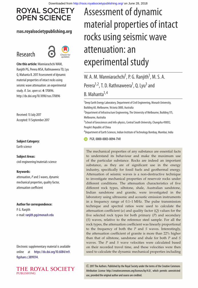
The mechanical properties of any substance are essential factsto understand its behaviour and make the maximum useof the particular substance. Rocks are indeed an importantsubstance, as they are of significant use in the energyindustry, specifically for fossil fuels and geothermal energy.Attenuation of seismic waves is a non-destructive techniqueto investigate mechanical properties of reservoir rocks underdifferent conditions. The attenuation characteristics of fivedifferent rock types, siltstone, shale, Australian sandstone,Indian sandstone and granite, were investigated in thelaboratory using ultrasonic and acoustic emission instrumentsin a frequency range of 0.1–1 MHz. The pulse transmissiontechnique and spectral ratios were used to calculate theattenuation coefficient (α) and quality factor (Q) values for thefive selected rock types for both primary (P) and secondary(S) waves, relative to the reference steel sample. For all therock types, the attenuation coefficient was linearly proportionalto the frequency of both the P and S waves. Interestingly,the attenuation coefficient of granite is more than 22% higherthan that of siltstone, sandstone and shale for both P and Swaves. The P and S wave velocities were calculated basedon their recorded travel time, and these velocities were thenused to calculate the dynamic mechanical properties including

2017 The Authors. Published by the Royal Society under the terms of the Creative CommonsAttribution License http://creativecommons.org/licenses/by/4.0/, which permits unrestricteduse, provided the original author and source are credited.

on June 28, 2018http://rsos.royalsocietypublishing.org/Downloaded from

2

rsos.royalsocietypublishing.orgR.Soc.opensci.4:170896

................................................elastic modulus (E), bulk modulus (K), shear modulus (µ) and Poisson’s ratio (ν). The P and S wavevelocities for the selected rock types varied in the ranges of 2.43–4.61 km s−1 and 1.43–2.41 km h−1,respectively. Furthermore, it was observed that the P wave velocity was always greater than theS wave velocity, and this confirmed the first arrival of P waves to the sensor. According to theexperimental results, the dynamic E value is generally higher than the static E value obtained byunconfined compressive strength tests.

1. IntroductionUnderstanding of the material properties of a substance is crucial to investigate the physical, chemicaland thermal behaviours associated with it. Therefore, over the past decades, researchers have studieddifferent types of materials to evaluate their usage in a broad range of applications. Among the differenttypes of substances, rocks have a significant place, due to their applications in various disciplinesincluding the energy sector, specifically in fossil fuels [1]. Considering energy and the environment, coalbed methane extraction [2], CO2 sequestration in deep geological formations [3], hydraulic fracturingof deep unconventional reservoirs [4,5] and deep geothermal energy [6] play important roles. All ofthe above-described processes are highly dependent on the material properties of the reservoir rock,which also varies highly with factors such as saturation medium, the degree of saturation, mineralcomposition of the rock and in situ stress conditions [7–9]. Well-bore drilling and hydraulic fracturingare two main processes associated with petroleum extraction and geothermal energy extraction [10],which are significantly affected by the strength properties of the rock [11]. In fact, it is a well-known factthat deep geological formations are formed according to different types of rock layers, and the materialproperties of these rocks are significantly different from each other. This makes fossil fuel explorationmore difficult due to the fact that the drilling and fracturing processes need to consider all the existingrock materials. Therefore, fossil fuel and geothermal energy extraction are heavily dependent on themechanical properties and saturation condition of the reservoir rocks, and precise knowledge of insitu mechanical properties and the saturation condition has become essential for effective fossil fueland energy extraction. Therefore, researchers and scientists are increasingly investigating reservoir rockproperties, specifically their strength and elastic properties, to make the fossil fuel and geothermal energyextraction more efficient and economical [7,12,13].

Various techniques are currently being used, and attenuation of seismic waves is a non-destructivetechnique [14] that can be used to investigate the mechanical properties of reservoir rocks as well asother substances [15]. Biwa [14] has studied the attenuation of waves in fibre-reinforced viscoelasticcomposites and found that when the wavelength is larger than the fibre radius, the attenuation coefficientis small compared with the viscoelastic matrix. Moreover, Pandit et al. [15] have characterized the waveattenuation in an elastic medium with voids and concluded that in elastic mediums with voids morethan one wavefront might exist. Seismic waves can be used to investigate the mechanical properties of thereservoir rock as well as to identify the optimal drilling locations [16,17]. Chai et al. [17] confirmed that therock joint properties including density and stiffness could be evaluated using seismic wave attenuation.Also, Jiang & Spikes [16] have developed a new procedure for seismic reservoir characterization andto locate optimum drilling locations. Body waves have a higher frequency and therefore travel fasterthan surface waves, and can be used to quantify the mechanical properties of rocks [18]. Body wavescan be subdivided into two main types: P waves (primary or compressional waves) and S waves(secondary or shear waves). The attenuation of P and S waves in rocks depends on many factors,including the physical state and saturation condition of the rocks [19,20]. Under laboratory conditions,the attenuation characteristics of rocks can be measured using several techniques, including the resonantbar technique [21–23], amplitude decay of multiple reflections [24], slow stress–strain cycling [25] andpulse transmission [26–28].

To date, a number of studies have been conducted on the mechanical properties of different rocksunder different saturation conditions using seismic waves. For example, Rathnaweera et al. [29] studiedthe attenuation of seismic waves in brine-saturated sandstone and found that attenuations in waterand 10% NaCl saturated sandstone are similar. Moreover, according to Johnston et al. [30], propertiesincluding the number of cracks, distribution of cracks, type of pore fluid, fluid saturation and themechanical properties of the rocks affect the attenuation of seismic waves in them. In addition, Johnstonet al. [30] observed that in dry rocks the attenuation is less than that in saturated rocks. Even though mostof the previous studies focused on P and S waves, Xia et al. [31] developed a new method to determine

on June 28, 2018http://rsos.royalsocietypublishing.org/Downloaded from

3

rsos.royalsocietypublishing.orgR.Soc.opensci.4:170896

................................................the quality factor for shear waves (Qs) using love waves. Bai [32] studied the correlation between thesonic velocity and rock density for different fields, and conducted a statistical analysis to evaluate therock density using sonic velocity. Furthermore, many studies have been carried out on attenuationcharacteristics of other geo-materials such as sand and clay. As an example, Darendeli [33] has conducteda study on dynamic properties and behaviour of clay soils due to ground vibration and developed a setof empirical curves for seismic site response analysis. In addition, Payan et al. [34] studied the effectof particle shape on the damping ratio of soils due to free vibration and developed an expression for thedamping ratio of soils subjected to confining stress.

However, because there have been very few studies related to the attenuation characteristics of dryrocks, understanding of the attenuation characteristics of different rock types remains limited. Therefore,a series of pulse transmission tests were conducted using acoustic emission (AE) and ultrasonic(UT) systems to investigate the attenuation characteristics of five different rock types: siltstone, shale,Australian sandstone, Indian sandstone and granite. The dynamic mechanical properties were alsocalculated, based on the seismic velocities (P and S), which can be used to identify the natural reservoirrock type prior to starting any fracturing or gas extraction process.

2. Experimental methodology2.1. Sample preparationFor this study, five different types of samples were selected: siltstone, shale, Australian sandstone, Indiansandstone and granite. The selected samples cover two different continents, and the details of the geologyof the samples are given in table 1. Rock samples were selected from five different basins in Australia,China and India. The geological maps of some of the basins are provided in the electronic supplementarymaterial. It should be noted that all the rock samples were taken from outcrops and when selecting thesamples, homogeneous samples were selected as much as possible to avoid the effect of existing layers.

Sample preparation and all the experiments were conducted in the Deep Earth Energy ResearchLaboratory of the Civil Engineering Department at Monash University. Samples were first cored into38 mm cylindrical shapes and then cut into 76 mm lengths. Both end surfaces of the samples werecarefully ground using a diamond grinding machine to produce parallel surfaces. Prepared samples werethen oven-dried for 48 h at 35°C to remove the moisture. It should be noted that because the samples weretaken from different basins, the natural moisture contents were different and this could affect the waveattenuation. Therefore, all the samples were oven-dried to remove the moisture. Prepared samples withtheir geographical origins are presented in table 1.

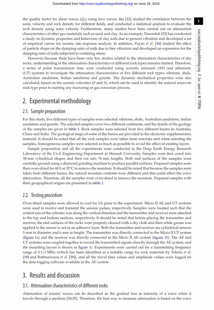
2.2. Testing procedureOven-dried samples were allowed to cool for 2 h prior to the experiment. Micro II AE and UT systemswere used to receive and transmit the seismic pulses, respectively. Samples were located such that thecentral axis of the cylinder was along the vertical direction and the transmitter and receiver were attachedto the top and bottom surfaces, respectively. It should be noted that before placing the transmitter andreceiver, the end surfaces of the rocks were properly cleaned with a dry cloth and then white grease wasapplied to the sensor to act as an adhesive layer. Both the transmitter and receiver are cylindrical sensors5 mm in diameter and 6 mm in height. The transmitter was directly connected to the Micro II UT system(figure 1a) and the receiver was directly connected to the Micro II AE system (figure 1b). The AE andUT systems were coupled together to record the transmitted signals directly through the AE system, andthe mounting layout is shown in figure 1c. Experiments were carried out for a transmitting frequencyrange of 0.1–1 MHz (which has been identified as a suitable range for rock materials by Toksöz et al.[19] and Rathnaweera et al. [29]), and all the travel time values and amplitude values were logged onthe data-logging software available in the AE system.

3. Results and discussion3.1. Attenuation characteristics of different rocksAttenuation of seismic waves can be described as the gradual loss in intensity of a wave when ittravels through a medium [18,35]. Therefore, the best way to measure attenuation is based on the wave

on June 28, 2018http://rsos.royalsocietypublishing.org/Downloaded from

4

rsos.royalsocietypublishing.orgR.Soc.opensci.4:170896

................................................

AE unit

UT unit

loggingthe time

transmitter

receiver

sample

(a) (b) (c)

Figure 1. (a) Micro II UT system, (b) Micro II AE system and (c) mounting layout of the transmitter and the receiver.

Table 1. Selected samples with geographical locations.

rock type location image detailssiltstone Eidsvold basin, Queensland

Australia— outcrop— formed in the Triassic, Jurassic

and Cretaceous periods— almost homogeneous— no visible layers

. . . . . . . . . . . . . . . . . . . . . . . . . . . . . . . . . . . . . . . . . . . . . . . . . . . . . . . . . . . . . . . . . . . . . . . . . . . . . . . . . . . . . . . . . . . . . . . . . . . . . . . . . . . . . . . . . . . . . . . . . . . . . . . . . . . . . . . . . . . . . . . . . . . . . . . . . . . . . . . . . . . . . . . . . . . . . . . . . . . . . . . . . . . . . . . . . . . . . . . . . . . . . . . . . . . . . . . . .

shale Lower Cambrian NiutitangFormation,North-Western HunanProvince, China

— outcrop— formed in the early Cambrian

period— organic rich black shale— no visible layers

. . . . . . . . . . . . . . . . . . . . . . . . . . . . . . . . . . . . . . . . . . . . . . . . . . . . . . . . . . . . . . . . . . . . . . . . . . . . . . . . . . . . . . . . . . . . . . . . . . . . . . . . . . . . . . . . . . . . . . . . . . . . . . . . . . . . . . . . . . . . . . . . . . . . . . . . . . . . . . . . . . . . . . . . . . . . . . . . . . . . . . . . . . . . . . . . . . . . . . . . . . . . . . . . . . . . . . . . .

sandstone (Ind) Dholpur, Rajasthan state,India

— outcrop— geology belongs to the Upper

Bhander group— medium-grained sandstone— visible layers

. . . . . . . . . . . . . . . . . . . . . . . . . . . . . . . . . . . . . . . . . . . . . . . . . . . . . . . . . . . . . . . . . . . . . . . . . . . . . . . . . . . . . . . . . . . . . . . . . . . . . . . . . . . . . . . . . . . . . . . . . . . . . . . . . . . . . . . . . . . . . . . . . . . . . . . . . . . . . . . . . . . . . . . . . . . . . . . . . . . . . . . . . . . . . . . . . . . . . . . . . . . . . . . . . . . . . . . . .

sandstone (Aus) Gosford basin, New SouthWales, Australia

— outcrop— formed in the early Triassic

period— coarse-grained sandstone— no visible layers

. . . . . . . . . . . . . . . . . . . . . . . . . . . . . . . . . . . . . . . . . . . . . . . . . . . . . . . . . . . . . . . . . . . . . . . . . . . . . . . . . . . . . . . . . . . . . . . . . . . . . . . . . . . . . . . . . . . . . . . . . . . . . . . . . . . . . . . . . . . . . . . . . . . . . . . . . . . . . . . . . . . . . . . . . . . . . . . . . . . . . . . . . . . . . . . . . . . . . . . . . . . . . . . . . . . . . . . . .

granite Strathbogie batholith,Victoria, Australia

— outcrop— formation is a composite

granitoid intrusion body— coarse-grained— highly discordant

. . . . . . . . . . . . . . . . . . . . . . . . . . . . . . . . . . . . . . . . . . . . . . . . . . . . . . . . . . . . . . . . . . . . . . . . . . . . . . . . . . . . . . . . . . . . . . . . . . . . . . . . . . . . . . . . . . . . . . . . . . . . . . . . . . . . . . . . . . . . . . . . . . . . . . . . . . . . . . . . . . . . . . . . . . . . . . . . . . . . . . . . . . . . . . . . . . . . . . . . . . . . . . . . . . . . . . . . .

amplitude, and in this study the pulse transmission technique was used to measure the attenuationrelative to a reference sample of steel (compared to rock, steel has very low attenuation, and it can beused as a reference to quantify the attenuation of different rocks). Therefore, all the experiments wereconducted using identical procedures for all the rock samples as well as the steel sample to calculatethe attenuation parameters. The amplitude of a plain seismic wave can be expressed as a function offrequency as follows [36]:

AS( f ) = GS(x) e−αS( f )xei(2π ft−kSx) (3.1)

and

AR( f ) = GR(x) e−αR( f )xei(2π ft−kRx), (3.2)

on June 28, 2018http://rsos.royalsocietypublishing.org/Downloaded from

5

rsos.royalsocietypublishing.orgR.Soc.opensci.4:170896

................................................

1.65

1.70

1.75

1.80

1.85

1.90

1.95

2.00

2.05

0 0.2 0.4 0.6 0.8 1.0

frequency (MHz)

0 0.2 0.4 0.6 0.8 1.0

frequency (MHz)

siltstoneshalesandstone (Ind)sandstone (Aus)granite

1.30

1.40

1.50

1.60

1.70

1.80

1.90

2.00

log

ampl

itude

(a) (b)

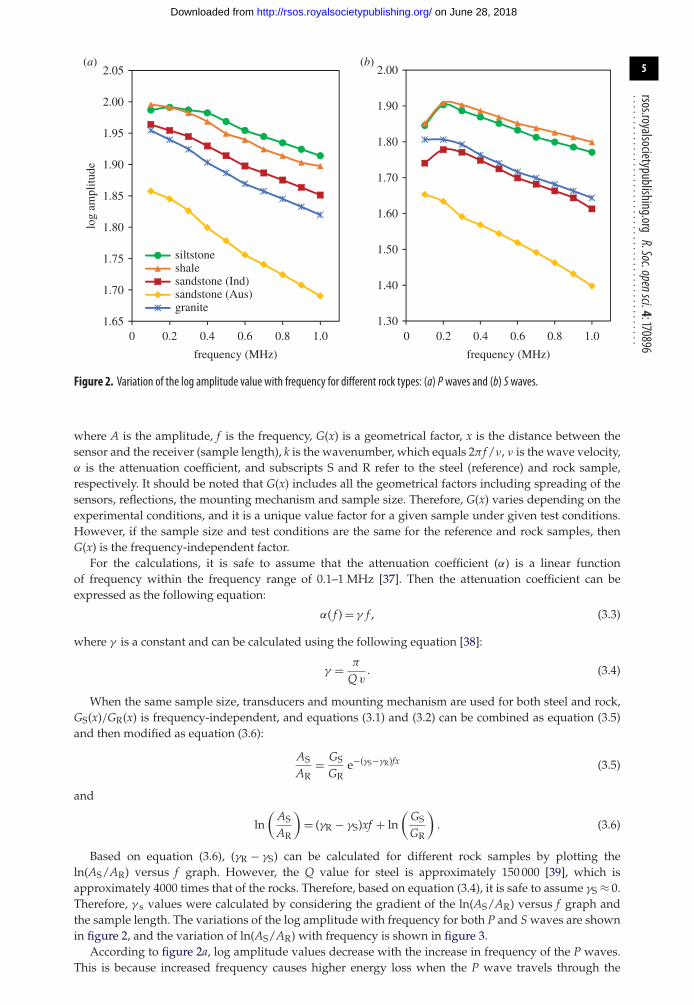
Figure 2. Variation of the log amplitude value with frequency for different rock types: (a) Pwaves and (b) Swaves.

where A is the amplitude, f is the frequency, G(x) is a geometrical factor, x is the distance between thesensor and the receiver (sample length), k is the wavenumber, which equals 2π f /ν, ν is the wave velocity,α is the attenuation coefficient, and subscripts S and R refer to the steel (reference) and rock sample,respectively. It should be noted that G(x) includes all the geometrical factors including spreading of thesensors, reflections, the mounting mechanism and sample size. Therefore, G(x) varies depending on theexperimental conditions, and it is a unique value factor for a given sample under given test conditions.However, if the sample size and test conditions are the same for the reference and rock samples, thenG(x) is the frequency-independent factor.

For the calculations, it is safe to assume that the attenuation coefficient (α) is a linear functionof frequency within the frequency range of 0.1–1 MHz [37]. Then the attenuation coefficient can beexpressed as the following equation:

α( f ) = γ f , (3.3)

where γ is a constant and can be calculated using the following equation [38]:

γ = π

Q v. (3.4)

When the same sample size, transducers and mounting mechanism are used for both steel and rock,GS(x)/GR(x) is frequency-independent, and equations (3.1) and (3.2) can be combined as equation (3.5)and then modified as equation (3.6):

AS

AR= GS

GRe−(γS−γR)fx (3.5)

and

ln(

AS

AR

)= (γR − γS)xf + ln

(GS

GR

). (3.6)

Based on equation (3.6), (γR − γS) can be calculated for different rock samples by plotting theln(AS/AR) versus f graph. However, the Q value for steel is approximately 150 000 [39], which isapproximately 4000 times that of the rocks. Therefore, based on equation (3.4), it is safe to assume γS ≈ 0.Therefore, γ s values were calculated by considering the gradient of the ln(AS/AR) versus f graph andthe sample length. The variations of the log amplitude with frequency for both P and S waves are shownin figure 2, and the variation of ln(AS/AR) with frequency is shown in figure 3.

According to figure 2a, log amplitude values decrease with the increase in frequency of the P waves.This is because increased frequency causes higher energy loss when the P wave travels through the

on June 28, 2018http://rsos.royalsocietypublishing.org/Downloaded from

6

rsos.royalsocietypublishing.orgR.Soc.opensci.4:170896

................................................

0

0.5

1.0

1.5

2.0

2.5

3.0

3.5

0 0.2 0.4 0.6 0.8 1.0 1.2

ln(A

stee

l/Aro

ck)

frequency (MHz)

0 0.2 0.4 0.6 0.8 1.0 1.2

frequency (MHz)

siltstoneshalesandstone (Ind)sandstone (Aus)granite

0

1

2

3

4

5

6

7

8(a) (b)

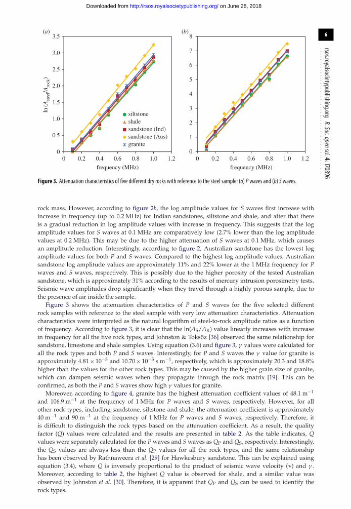
Figure 3. Attenuation characteristics of five different dry rocks with reference to the steel sample: (a) Pwaves and (b) Swaves.

rock mass. However, according to figure 2b, the log amplitude values for S waves first increase withincrease in frequency (up to 0.2 MHz) for Indian sandstones, siltstone and shale, and after that thereis a gradual reduction in log amplitude values with increase in frequency. This suggests that the logamplitude values for S waves at 0.1 MHz are comparatively low (2.7% lower than the log amplitudevalues at 0.2 MHz). This may be due to the higher attenuation of S waves at 0.1 MHz, which causesan amplitude reduction. Interestingly, according to figure 2, Australian sandstone has the lowest logamplitude values for both P and S waves. Compared to the highest log amplitude values, Australiansandstone log amplitude values are approximately 11% and 22% lower at the 1 MHz frequency for Pwaves and S waves, respectively. This is possibly due to the higher porosity of the tested Australiansandstone, which is approximately 31% according to the results of mercury intrusion porosimetry tests.Seismic wave amplitudes drop significantly when they travel through a highly porous sample, due tothe presence of air inside the sample.

Figure 3 shows the attenuation characteristics of P and S waves for the five selected differentrock samples with reference to the steel sample with very low attenuation characteristics. Attenuationcharacteristics were interpreted as the natural logarithm of steel-to-rock amplitude ratios as a functionof frequency. According to figure 3, it is clear that the ln(AS/AR) value linearly increases with increasein frequency for all the five rock types, and Johnston & Toksöz [36] observed the same relationship forsandstone, limestone and shale samples. Using equation (3.6) and figure 3, γ values were calculated forall the rock types and both P and S waves. Interestingly, for P and S waves the γ value for granite isapproximately 4.81 × 10−5 and 10.70 × 10−5 s m−1, respectively, which is approximately 20.3 and 18.8%higher than the values for the other rock types. This may be caused by the higher grain size of granite,which can dampen seismic waves when they propagate through the rock matrix [19]. This can beconfirmed, as both the P and S waves show high γ values for granite.

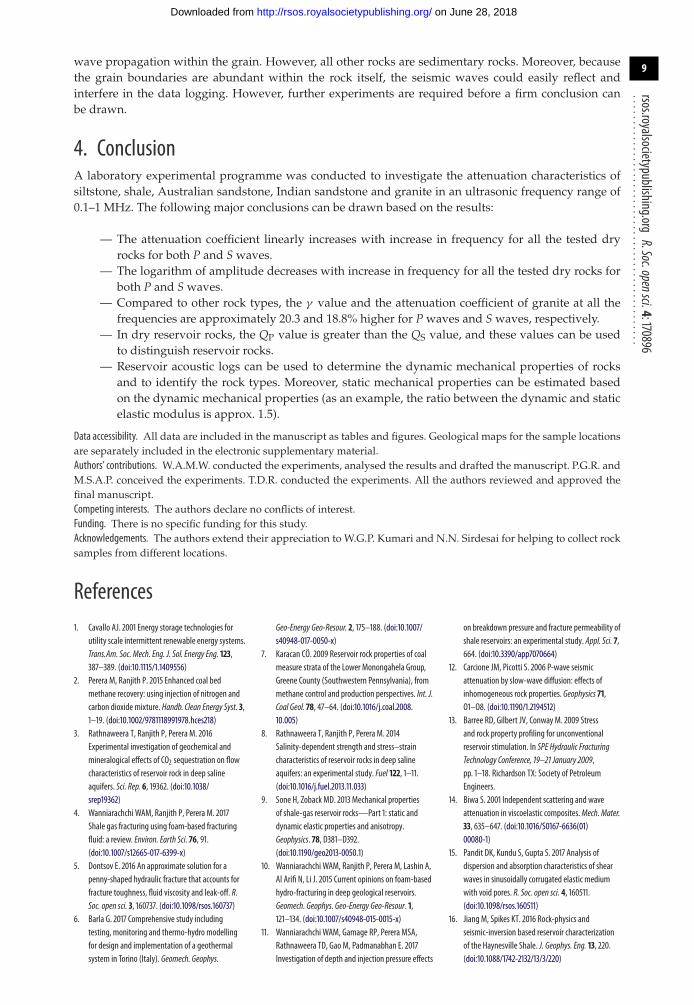
Moreover, according to figure 4, granite has the highest attenuation coefficient values of 48.1 m−1

and 106.9 m−1 at the frequency of 1 MHz for P waves and S waves, respectively. However, for allother rock types, including sandstone, siltstone and shale, the attenuation coefficient is approximately40 m−1 and 90 m−1 at the frequency of 1 MHz for P waves and S waves, respectively. Therefore, itis difficult to distinguish the rock types based on the attenuation coefficient. As a result, the qualityfactor (Q) values were calculated and the results are presented in table 2. As the table indicates, Qvalues were separately calculated for the P waves and S waves as QP and QS, respectively. Interestingly,the QS values are always less than the QP values for all the rock types, and the same relationshiphas been observed by Rathnaweera et al. [29] for Hawkesbury sandstone. This can be explained usingequation (3.4), where Q is inversely proportional to the product of seismic wave velocity (ν) and γ .Moreover, according to table 2, the highest Q value is observed for shale, and a similar value wasobserved by Johnston et al. [30]. Therefore, it is apparent that QP and QS can be used to identify therock types.

on June 28, 2018http://rsos.royalsocietypublishing.org/Downloaded from

7

rsos.royalsocietypublishing.orgR.Soc.opensci.4:170896

................................................

0

10

20

30

40

50

60

0 0.2 0.4 0.6 0.8 1.0 1.2 0 0.2 0.4 0.6 0.8 1.0 1.2

atte

nuat

ion

coef

fici

ent (

m–1

)

frequency (MHz) frequency (MHz)

siltstoneshalesandstone (Ind)sandstone (Aus)granite

0

20

40

60

80

100

120(a) (b)

Figure 4. Variation of attenuation coefficient with frequency for different types of rocks: (a) P waves and (b) Swaves.

Table 2. Calculated quality factor (Q) values for P waves and S waves.

QP QS

rock type mean valuestandarddeviation mean value

standarddeviation

siltstone 21.11 0.47 16.15 0.60. . . . . . . . . . . . . . . . . . . . . . . . . . . . . . . . . . . . . . . . . . . . . . . . . . . . . . . . . . . . . . . . . . . . . . . . . . . . . . . . . . . . . . . . . . . . . . . . . . . . . . . . . . . . . . . . . . . . . . . . . . . . . . . . . . . . . . . . . . . . . . . . . . . . . . . . . . . . . . . . . . . . . . . . . . . . . . . . . . . . . . . . . . . . . . . . . . . . . . . . . . . . . . . . . . . . . . . . .

shale 32.16 0.36 24.72 0.73. . . . . . . . . . . . . . . . . . . . . . . . . . . . . . . . . . . . . . . . . . . . . . . . . . . . . . . . . . . . . . . . . . . . . . . . . . . . . . . . . . . . . . . . . . . . . . . . . . . . . . . . . . . . . . . . . . . . . . . . . . . . . . . . . . . . . . . . . . . . . . . . . . . . . . . . . . . . . . . . . . . . . . . . . . . . . . . . . . . . . . . . . . . . . . . . . . . . . . . . . . . . . . . . . . . . . . . . .

sandstone (Ind) 25.77 0.40 19.63 3.29. . . . . . . . . . . . . . . . . . . . . . . . . . . . . . . . . . . . . . . . . . . . . . . . . . . . . . . . . . . . . . . . . . . . . . . . . . . . . . . . . . . . . . . . . . . . . . . . . . . . . . . . . . . . . . . . . . . . . . . . . . . . . . . . . . . . . . . . . . . . . . . . . . . . . . . . . . . . . . . . . . . . . . . . . . . . . . . . . . . . . . . . . . . . . . . . . . . . . . . . . . . . . . . . . . . . . . . . .

sandstone (Aus) 28.17 0.72 23.08 1.22. . . . . . . . . . . . . . . . . . . . . . . . . . . . . . . . . . . . . . . . . . . . . . . . . . . . . . . . . . . . . . . . . . . . . . . . . . . . . . . . . . . . . . . . . . . . . . . . . . . . . . . . . . . . . . . . . . . . . . . . . . . . . . . . . . . . . . . . . . . . . . . . . . . . . . . . . . . . . . . . . . . . . . . . . . . . . . . . . . . . . . . . . . . . . . . . . . . . . . . . . . . . . . . . . . . . . . . . .

granite 14.15 4.41 12.21 1.09. . . . . . . . . . . . . . . . . . . . . . . . . . . . . . . . . . . . . . . . . . . . . . . . . . . . . . . . . . . . . . . . . . . . . . . . . . . . . . . . . . . . . . . . . . . . . . . . . . . . . . . . . . . . . . . . . . . . . . . . . . . . . . . . . . . . . . . . . . . . . . . . . . . . . . . . . . . . . . . . . . . . . . . . . . . . . . . . . . . . . . . . . . . . . . . . . . . . . . . . . . . . . . . . . . . . . . . . .

3.2. Dynamic mechanical properties of different rocksThe mechanical properties of a reservoir rock, including elastic modulus (E), bulk modulus (K), shearmodulus (µ) and Poisson’s ratio (ν), can be calculated as static or dynamic properties [40]. Staticmechanical properties can be calculated from tri-axial or uni-axial tests (static tests), and dynamicmechanical properties can be calculated using seismic waves. In this study, dynamic mechanicalproperties were calculated using equations (3.7)–(3.10), based on the density, and P wave and S wavevelocities [41–43]. The calculated dynamic mechanical properties are presented in table 3.

E = ρ v2S(3v2

P − 4v2s )

v2P − v2

s, (3.7)

K = ρ

(v2

P − 43v2

s

), (3.8)

μ = ρ v2s (3.9)

and υ = v2P − 2v2

s

2(v2P − v2

s ), (3.10)

where E is the dynamic elastic modulus, K is the dynamic bulk modulus, µ is the dynamic shear modulus,υ is the dynamic Poisson’s ratio, ρ is the rock density, νP is the P wave velocity and νS is the S wavevelocity.

on June 28, 2018http://rsos.royalsocietypublishing.org/Downloaded from

8

rsos.royalsocietypublishing.orgR.Soc.opensci.4:170896

................................................Table 3. Seismic wave velocities and dynamic mechanical properties of different rocks (note that dynamic mechanical properties werecalculated based on the mean velocity values).

Vp (km s−1) Vs (km s−1)

rock typemeanvalue

standarddeviation

meanvalue

standarddeviation ρ (kg m−3) E (GPa) K (GPa) µ (GPa) ν

siltstone 3.73 0.08 2.14 0.08 2239 25.80 17.35 10.30 0.25. . . . . . . . . . . . . . . . . . . . . . . . . . . . . . . . . . . . . . . . . . . . . . . . . . . . . . . . . . . . . . . . . . . . . . . . . . . . . . . . . . . . . . . . . . . . . . . . . . . . . . . . . . . . . . . . . . . . . . . . . . . . . . . . . . . . . . . . . . . . . . . . . . . . . . . . . . . . . . . . . . . . . . . . . . . . . . . . . . . . . . . . . . . . . . . . . . . . . . . . . . . . . . . . . . . . . . . . .

shale 2.43 0.03 1.43 0.04 2661 13.45 8.39 5.46 0.23. . . . . . . . . . . . . . . . . . . . . . . . . . . . . . . . . . . . . . . . . . . . . . . . . . . . . . . . . . . . . . . . . . . . . . . . . . . . . . . . . . . . . . . . . . . . . . . . . . . . . . . . . . . . . . . . . . . . . . . . . . . . . . . . . . . . . . . . . . . . . . . . . . . . . . . . . . . . . . . . . . . . . . . . . . . . . . . . . . . . . . . . . . . . . . . . . . . . . . . . . . . . . . . . . . . . . . . . .

sandstone (Ind) 3.11 0.05 1.82 0.25 2198 18.10 11.54 7.30 0.24. . . . . . . . . . . . . . . . . . . . . . . . . . . . . . . . . . . . . . . . . . . . . . . . . . . . . . . . . . . . . . . . . . . . . . . . . . . . . . . . . . . . . . . . . . . . . . . . . . . . . . . . . . . . . . . . . . . . . . . . . . . . . . . . . . . . . . . . . . . . . . . . . . . . . . . . . . . . . . . . . . . . . . . . . . . . . . . . . . . . . . . . . . . . . . . . . . . . . . . . . . . . . . . . . . . . . . . . .

sandstone (Aus) 2.71 0.07 1.49 0.08 2202 12.59 9.65 4.91 0.28. . . . . . . . . . . . . . . . . . . . . . . . . . . . . . . . . . . . . . . . . . . . . . . . . . . . . . . . . . . . . . . . . . . . . . . . . . . . . . . . . . . . . . . . . . . . . . . . . . . . . . . . . . . . . . . . . . . . . . . . . . . . . . . . . . . . . . . . . . . . . . . . . . . . . . . . . . . . . . . . . . . . . . . . . . . . . . . . . . . . . . . . . . . . . . . . . . . . . . . . . . . . . . . . . . . . . . . . .

granite 4.61 1.31 2.41 0.21 2616 39.78 35.42 15.15 0.31. . . . . . . . . . . . . . . . . . . . . . . . . . . . . . . . . . . . . . . . . . . . . . . . . . . . . . . . . . . . . . . . . . . . . . . . . . . . . . . . . . . . . . . . . . . . . . . . . . . . . . . . . . . . . . . . . . . . . . . . . . . . . . . . . . . . . . . . . . . . . . . . . . . . . . . . . . . . . . . . . . . . . . . . . . . . . . . . . . . . . . . . . . . . . . . . . . . . . . . . . . . . . . . . . . . . . . . . .

Table 4. Comparison of dynamic and static elastic modulus (Ed and Es) and Poisson’s ratio (υd and υ s) for different rocks (note thatdynamic mechanical properties were calculated based on the mean velocity values).

Estatic (GPa) νstatic

rock typeEdynamic(GPa)

meanvalue

standarddeviation Ed/Es νdynamic

meanvalue

standarddeviation νd/νs

siltstone 25.80 16.00 0.32 1.61 0.25 0.30 0.01 0.84. . . . . . . . . . . . . . . . . . . . . . . . . . . . . . . . . . . . . . . . . . . . . . . . . . . . . . . . . . . . . . . . . . . . . . . . . . . . . . . . . . . . . . . . . . . . . . . . . . . . . . . . . . . . . . . . . . . . . . . . . . . . . . . . . . . . . . . . . . . . . . . . . . . . . . . . . . . . . . . . . . . . . . . . . . . . . . . . . . . . . . . . . . . . . . . . . . . . . . . . . . . . . . . . . . . . . . . . .

shale 13.45 7.56 0.14 1.78 0.23 0.21 0.02 1.11. . . . . . . . . . . . . . . . . . . . . . . . . . . . . . . . . . . . . . . . . . . . . . . . . . . . . . . . . . . . . . . . . . . . . . . . . . . . . . . . . . . . . . . . . . . . . . . . . . . . . . . . . . . . . . . . . . . . . . . . . . . . . . . . . . . . . . . . . . . . . . . . . . . . . . . . . . . . . . . . . . . . . . . . . . . . . . . . . . . . . . . . . . . . . . . . . . . . . . . . . . . . . . . . . . . . . . . . .

sandstone (Ind) 18.10 11 0.21 1.65 0.24 0.31 0.01 0.77. . . . . . . . . . . . . . . . . . . . . . . . . . . . . . . . . . . . . . . . . . . . . . . . . . . . . . . . . . . . . . . . . . . . . . . . . . . . . . . . . . . . . . . . . . . . . . . . . . . . . . . . . . . . . . . . . . . . . . . . . . . . . . . . . . . . . . . . . . . . . . . . . . . . . . . . . . . . . . . . . . . . . . . . . . . . . . . . . . . . . . . . . . . . . . . . . . . . . . . . . . . . . . . . . . . . . . . . .

sandstone (Aus) 12.59 10.29 0.68 1.22 0.28 0.26 0.02 1.09. . . . . . . . . . . . . . . . . . . . . . . . . . . . . . . . . . . . . . . . . . . . . . . . . . . . . . . . . . . . . . . . . . . . . . . . . . . . . . . . . . . . . . . . . . . . . . . . . . . . . . . . . . . . . . . . . . . . . . . . . . . . . . . . . . . . . . . . . . . . . . . . . . . . . . . . . . . . . . . . . . . . . . . . . . . . . . . . . . . . . . . . . . . . . . . . . . . . . . . . . . . . . . . . . . . . . . . . .

granite 39.78 12.13 0.81 3.28 0.31 0.20 0.02 1.56. . . . . . . . . . . . . . . . . . . . . . . . . . . . . . . . . . . . . . . . . . . . . . . . . . . . . . . . . . . . . . . . . . . . . . . . . . . . . . . . . . . . . . . . . . . . . . . . . . . . . . . . . . . . . . . . . . . . . . . . . . . . . . . . . . . . . . . . . . . . . . . . . . . . . . . . . . . . . . . . . . . . . . . . . . . . . . . . . . . . . . . . . . . . . . . . . . . . . . . . . . . . . . . . . . . . . . . . .

According to table 3, the νP values are always higher than the νS values, because the travel timefor P waves is less than that for S waves. Moreover, the obtained P and S wave velocities are withinthe range of 2–5 km s−1, which is consistent with the values obtained by Mavko [44]. Moreover, theE values and υ values are within the range of 10–40 GPa and 0.2–0.32 GPa, respectively, which isacceptable for rock materials [45]. Furthermore, the obtained values for K and µ are consistent withthe values obtained by Toksöz et al. [41] for sandstone and granite. Therefore, it is evident that the Pand S wave velocities can be used to calculate the dynamic mechanical properties of the five testedrock types. As can be seen in table 3, P and S wave velocities for Australian and Indian sandstonesare quite different. This could be mainly due to the mineralogical contents of the two sandstones, withthe quartz content approximately 85% and 95% in Australian and Indian sandstones, respectively. Inaddition, considering the grain size, Australian sandstone is a coarse-grained sandstone (grain size inthe range of 0.04–1.0 mm), and the Indian sandstone is about fine- to medium-grained. Therefore, thesedifferences may cause the significant variation between the P and S wave velocities in sandstones fromthe two continents. Table 4 gives a comparison of the dynamic and static elastic modulus and Poisson’sratio for the selected rock types. It should be noted that the static mechanical properties have been testedin the laboratory under previous studies, and further details can be found in Rathnaweera et al. [8],Sirdesai et al. [46] and Kumari et al. [47]. According to table 4, the dynamic elastic modulus is alwaysgreater than the static elastic modulus for all the tested rock types. This has also been observed by Yale[40] for dolostone, limestone, siltstone and mudstone. Moreover, the dynamic elastic modulus valuesof the siltstone, shale and sandstone are 22–78% higher than those of the static elastic modulus values,which is consistent with the range (15–70%) observed by Yale [40]. Furthermore, the ratio between thedynamic and static elastic modulus values is approximately 1.5. The higher dynamic elastic modulusvalues may be caused by geometric spreading, reflections, scattering and intrinsic damping, whichcan happen during wave propagation. However, according to table 4, granite has the highest dynamicelastic modulus, which is approximately 230% greater than the static elastic modulus. This may be dueto the higher grain size of the granite, which may interfere in the propagation of seismic waves. Inaddition, granite is a crystalline rock with large grains (visible to naked eye), and this could enhance the

on June 28, 2018http://rsos.royalsocietypublishing.org/Downloaded from

9

rsos.royalsocietypublishing.orgR.Soc.opensci.4:170896

................................................wave propagation within the grain. However, all other rocks are sedimentary rocks. Moreover, becausethe grain boundaries are abundant within the rock itself, the seismic waves could easily reflect andinterfere in the data logging. However, further experiments are required before a firm conclusion canbe drawn.

4. ConclusionA laboratory experimental programme was conducted to investigate the attenuation characteristics ofsiltstone, shale, Australian sandstone, Indian sandstone and granite in an ultrasonic frequency range of0.1–1 MHz. The following major conclusions can be drawn based on the results:

— The attenuation coefficient linearly increases with increase in frequency for all the tested dryrocks for both P and S waves.

— The logarithm of amplitude decreases with increase in frequency for all the tested dry rocks forboth P and S waves.

— Compared to other rock types, the γ value and the attenuation coefficient of granite at all thefrequencies are approximately 20.3 and 18.8% higher for P waves and S waves, respectively.

— In dry reservoir rocks, the QP value is greater than the QS value, and these values can be usedto distinguish reservoir rocks.

— Reservoir acoustic logs can be used to determine the dynamic mechanical properties of rocksand to identify the rock types. Moreover, static mechanical properties can be estimated basedon the dynamic mechanical properties (as an example, the ratio between the dynamic and staticelastic modulus is approx. 1.5).

Data accessibility. All data are included in the manuscript as tables and figures. Geological maps for the sample locationsare separately included in the electronic supplementary material.Authors’ contributions. W.A.M.W. conducted the experiments, analysed the results and drafted the manuscript. P.G.R. andM.S.A.P. conceived the experiments. T.D.R. conducted the experiments. All the authors reviewed and approved thefinal manuscript.Competing interests. The authors declare no conflicts of interest.Funding. There is no specific funding for this study.Acknowledgements. The authors extend their appreciation to W.G.P. Kumari and N.N. Sirdesai for helping to collect rocksamples from different locations.

References1. Cavallo AJ. 2001 Energy storage technologies for

utility scale intermittent renewable energy systems.Trans.Am. Soc. Mech. Eng. J. Sol. Energy Eng. 123,387–389. (doi:10.1115/1.1409556)

2. Perera M, Ranjith P. 2015 Enhanced coal bedmethane recovery: using injection of nitrogen andcarbon dioxide mixture. Handb. Clean Energy Syst. 3,1–19. (doi:10.1002/9781118991978.hces218)

3. Rathnaweera T, Ranjith P, Perera M. 2016Experimental investigation of geochemical andmineralogical effects of CO2 sequestration on flowcharacteristics of reservoir rock in deep salineaquifers. Sci. Rep. 6, 19362. (doi:10.1038/srep19362)

4. Wanniarachchi WAM, Ranjith P, Perera M. 2017Shale gas fracturing using foam-based fracturingfluid: a review. Environ. Earth Sci. 76, 91.(doi:10.1007/s12665-017-6399-x)

5. Dontsov E. 2016 An approximate solution for apenny-shaped hydraulic fracture that accounts forfracture toughness, fluid viscosity and leak-off. R.Soc. open sci. 3, 160737. (doi:10.1098/rsos.160737)

6. Barla G. 2017 Comprehensive study includingtesting, monitoring and thermo-hydro modellingfor design and implementation of a geothermalsystem in Torino (Italy). Geomech. Geophys.

Geo-Energy Geo-Resour. 2, 175–188. (doi:10.1007/s40948-017-0050-x)

7. Karacan CÖ. 2009 Reservoir rock properties of coalmeasure strata of the Lower Monongahela Group,Greene County (Southwestern Pennsylvania), frommethane control and production perspectives. Int. J.Coal Geol. 78, 47–64. (doi:10.1016/j.coal.2008.10.005)

8. Rathnaweera T, Ranjith P, Perera M. 2014Salinity-dependent strength and stress–straincharacteristics of reservoir rocks in deep salineaquifers: an experimental study. Fuel 122, 1–11.(doi:10.1016/j.fuel.2013.11.033)

9. Sone H, Zoback MD. 2013 Mechanical propertiesof shale-gas reservoir rocks—Part 1: static anddynamic elastic properties and anisotropy.Geophysics. 78, D381–D392.(doi:10.1190/geo2013-0050.1)

10. Wanniarachchi WAM, Ranjith P, Perera M, Lashin A,Al Arifi N, Li J. 2015 Current opinions on foam-basedhydro-fracturing in deep geological reservoirs.Geomech. Geophys. Geo-Energy Geo-Resour. 1,121–134. (doi:10.1007/s40948-015-0015-x)

11. Wanniarachchi WAM, Gamage RP, Perera MSA,Rathnaweera TD, Gao M, Padmanabhan E. 2017Investigation of depth and injection pressure effects

on breakdown pressure and fracture permeability ofshale reservoirs: an experimental study. Appl. Sci. 7,664. (doi:10.3390/app7070664)

12. Carcione JM, Picotti S. 2006 P-wave seismicattenuation by slow-wave diffusion: effects ofinhomogeneous rock properties. Geophysics 71,O1–O8. (doi:10.1190/1.2194512)

13. Barree RD, Gilbert JV, Conway M. 2009 Stressand rock property profiling for unconventionalreservoir stimulation. In SPE Hydraulic FracturingTechnology Conference, 19–21 January 2009,pp. 1–18. Richardson TX: Society of PetroleumEngineers.

14. Biwa S. 2001 Independent scattering and waveattenuation in viscoelastic composites.Mech. Mater.33, 635–647. (doi:10.1016/S0167-6636(01)00080-1)

15. Pandit DK, Kundu S, Gupta S. 2017 Analysis ofdispersion and absorption characteristics of shearwaves in sinusoidally corrugated elastic mediumwith void pores. R. Soc. open sci. 4, 160511.(doi:10.1098/rsos.160511)

16. Jiang M, Spikes KT. 2016 Rock-physics andseismic-inversion based reservoir characterizationof the Haynesville Shale. J. Geophys. Eng. 13, 220.(doi:10.1088/1742-2132/13/3/220)

on June 28, 2018http://rsos.royalsocietypublishing.org/Downloaded from

10

rsos.royalsocietypublishing.orgR.Soc.opensci.4:170896

................................................17. Chai S, Li J, Rong L, Li N. 2017 Theoretical study for

induced seismic wave propagation across rockmasses during underground exploitation. Geomech.Geophys. Geo-Energy Geo-Resour. 2, 95–105.(doi:10.1007/s40948-016-0043-1)

18. Ben-Menahem A, Singh SJ. 2012 Seismic wavesand sources. Berlin, Germany: Springer Science &Business Media.

19. Toksöz MN, Johnston DH, Timur AT. 1979Attenuation of seismic waves in dry and saturatedrocks: I. Laboratory measurements. Geophysics 44,681–690. (doi:10.1190/1.1440969)

20. Feng Z, Mingjie X, Zhonggao M, Liang C, Zhu Z, JuanL. 2012 An experimental study on the correlationbetween the elastic wave velocity andmicrofractures in coal rock from the Qingshui basin.J. Geophys. Eng. 9, 691.(doi:10.1088/1742-2132/9/6/691)

21. Birch F, Bancroft D. 1938 Elasticity and internalfriction in a long column of granite. Bull. Seismol.Soc. Am. 28, 243–254.

22. Gardner G, Wyllie M, Droschak D. 1964 Effects ofpressure and fluid saturation on the attenuation ofelastic waves in sands. J. Pet. Technol. 16, 189–198.(doi:10.2118/721-PA)

23. Spetzler H, Anderson DL. 1968 The effect oftemperature and partial melting on velocity andattenuation in a simple binary system. J. Geophys.Res. 73, 6051–6060. (doi:10.1029/JB073i018p06051)

24. Peselnick L, Outerbridge W. 1961 Internal frictionand rigidity modulus of Solenhofen limestone overa wide frequency range. US Geol. Surv. Prof. Pap. B,400B.

25. Jackson DD. 2009 Grain boundary relaxation andattenuation of seismic waves. In Transactions,American Geophysical Union, January 1970, vol. 51,p. 204. Washington, DC: American GeophysicalUnion.

26. Kuster GT, Toksöz MN. 1974 Velocity and attenuationof seismic waves in two-phase media: Part II.experimental results. Geophysics 39, 607–618.(doi:10.1190/1.1440451)

27. Tittmann BR, Housley RM, Alers GA, Cirlin EH. 1974Internal friction in rocks and its relationship tovolatiles on the moon. In Lunar and PlanetaryScience Conference Proceedings,March 18–22, 1974,

pp. 2913–2918. New York, NY: Pergamon Press,Inc.

28. Watson T, Wuenschel P. 1973 An experimental studyof attenuation in fluid saturated porous media,compressional waves and interfacial waves. In Proc.43rd Annu. Intl SEG Meeting, 22 October 1973, MexicoCity, Mexico, pp. 22–35. Society of ExplorationGeophysicists.

29. Rathnaweera TD, Ranjith PG, Perera MSA. 2015Attenuation of seismic waves in brine-saturatedHawkesbury Sandstone: an experimental study.In 49th US Rock Mechanics/GeomechanicsSymposium, 28 June–1 July 2015, pp. 1–7. SanFrancisco, CA: American Rock MechanicsAssociation.

30. Johnston DH, Toksöz M, Timur A. 1979 Attenuationof seismic waves in dry and saturated rocks: II.Mechanisms. Geophysics 44, 691–711. (doi:10.1190/1.1440970)

31. Xia J, Yin X, Xu Y. 2013 Feasibility of determining Qof near-surface materials from love waves. J. Appl.Geophys. 95, 47–52. (doi:10.1016/j.jappgeo.2013.05.007)

32. Bai M. 2016 Mechanical characteristics oflaminated sand–shale sequences identifiedfrom sonic velocity and density correlations.Geomech. Geophys. Geo-Energy Geo-Resour.2, 275–300. (doi:10.1007/s40948-016-0036-0)

33. Darendeli MB. 2001 Development of a new familyof normalized modulus reduction and materialdamping curves. PhD thesis, University of Texas atAustin, Austin, TX. See https://utexas-ir.tdl.org/bitstream/handle/2152/10396/darendelimb016.pdf?sequence=4&isAllowed=y.

34. Payan M, Senetakis K, Khoshghalb A, Khalili N. 2016Influence of particle shape on small-strain dampingratio of dry sands. Géotechnique 66, 610–616.(doi:10.1680/jgeot.15.T.035)

35. Cavallini F. 1995 Attenuation and quality factorsurfaces in anisotropic-viscoelastic media.Mech.Mater. 19, 311–327. (doi:10.1016/0167-6636(94)00040-N)

36. Johnston DH, Toksöz MN. 1980 Ultrasonic P and Swave attenuation in dry and saturated rocks underpressure. J. Geophys. Res. Solid Earth 85, 925–936.(doi:10.1029/JB085iB02p00925)

37. Jackson DD, Anderson DL. 1970 Physicalmechanisms of seismic-wave attenuation. Rev.Geophys. 8, 1–63. (doi:10.1029/RG008i001p00001)

38. Liu C, Ahrens TJ. 1997 Stress wave attenuationin shock-damaged rock. J. Geophys. Res. 102,5243–5250. (doi:10.1029/96JB03891)

39. Zemanek Jr J, Rudnick I. 1961 Attenuation anddispersion of elastic waves in a cylindrical bar.J. Acoust. Soc. Am. 33, 1283–1288. (doi:10.1121/1.1908417)

40. Yale D. 1994 Static and dynamic rock mechanicalproperties in the Hugoton and Panoma fields,Kansas. In SPE Mid-Continent Gas Symposium,22–24 May, 1994. Amarillo, TX: Society of PetroleumEngineers.

41. Toksöz MN, Cheng CH, Timur A. 1976 Velocities ofseismic waves in porous rocks. Geophysics 41,621–645. (doi:10.1190/1.1440639)

42. Castagna JP, Batzle ML, Eastwood RL. 1985Relationships between compressional-wave andshear-wave velocities in clastic silicate rocks.Geophysics 50, 571–581. (doi:10.1190/1.1441933)

43. Wyllie MRJ, Gregory AR, Gardner LW. 1956 Elasticwave velocities in heterogeneous and porousmedia. Geophysics 21, 41–70. (doi:10.1190/1.1438217)

44. Mavko G. 2005 Conceptual overview of rock andfluid factors that impact seismic velocity andimpedance. Stanford Rock Physics Laboratory.Stanford School of Earth Sciences. See https://pangea.stanford.edu/courses/gp262/Notes/8.SeismicVelocity.pdf (accessed November 2012).

45. Lama R, Vutukuri V. 1978 Handbook on mechanicalproperties of rocks-testing techniques and results,vol. 2. Clausthal, Germany: Trans Tech Publications.

46. Sirdesai N, Singh T, Ranjith P, Singh R. 2017 Effectof varied durations of thermal treatment on thetensile strength of Red Sandstone. Rock Mech. RockEng. 50, 205–213. (doi:10.1007/s00603-016-1047-4)

47. Kumari WGP, Ranjith PG, Perera MSA, Shao S,Chen BK, Lashin A, Arifi NA, Rathnaweera TD. 2017Mechanical behaviour of Australian Strathbogiegranite under in-situ stress and temperatureconditions: an application to geothermal energyextraction. Geothermics 65, 44–59.(doi:10.1016/j.geothermics.2016.07.002)

on June 28, 2018http://rsos.royalsocietypublishing.org/Downloaded from