Assessment of the maximum loadability point of a power

Turk J Elec Eng & Comp Sci

(2016) 24: 4174 – 4192

c⃝ TUBITAK

doi:10.3906/elk-1404-511

Turkish Journal of Electrical Engineering & Computer Sciences

http :// journa l s . tub i tak .gov . t r/e lektr ik/

Research Article

Assessment of the maximum loadability point of a power system after third zone

of distance relay corrective actions

Zahra MORAVEJ∗, Sajad BAGHERIFaculty of Electrical and Computer Engineering, Semnan University, Semnan, Iran

Received: 24.04.2014 • Accepted/Published Online: 28.07.2015 • Final Version: 20.06.2016

Abstract: In this paper, the operation of a system and distance relay is improved during voltage instability by using

an improved strategy. After detecting the voltage instability, the third zone is blocked. However, the system is prone

to voltage collapse. Shunt capacitor compensation and a load shedding scheme can be used to protect the system from

voltage collapse conditions. Load shedding plans can be performed based on a reduction in the power flow in the line

where the relay is located. The reason is that the minimum eigenvalue of the load flow Jacobian (reduced and unreduced

Jacobians) is increased and the static voltage stability is improved. After the shunt capacitor compensation and load

shedding, the relay margin becomes positive, impedance comes out from the third zone, and the relay does not need to

remain blocked. The maximum loadability point (MLP) is increased by performing a control action in the system. To

accomplish this strategy, the 14-bus IEEE test system is used.

Key words: Voltage stability, distance protection, corrective action, power estimation, load flow Jacobian

1. Introduction

Voltage stability is one of the major issues for operators of power systems due to its importance in the field of

security and power quality of the systems. Voltage stability refers to the ability of a power system to maintain

steady voltages at all buses in the system after being subjected to a disturbance from a given initial operating

condition [1]. For convenience in analysis and for gaining useful insight into the nature of voltage stability

problems, it is useful to characterize voltage stability in terms of large-disturbance and small-disturbance voltage

stability. Large-disturbance voltage stability refers to the system’s ability to maintain steady voltages following

large disturbances such as system faults, loss of generation, or circuit contingencies. Small-disturbance voltage

stability considers the power system’s ability to control voltages after small disturbances, e.g., changes in

load. Voltage stability can be divided in terms of short-term and long-term events. In short-term voltage

stability, dynamics of fast-acting load components such as induction motors, electronically controlled loads, and

HVDC converters are considered. The time interval for the study of this kind of stability is approximately

several seconds, and it is done by solving differential equations of the system. Long-term voltage stability is

characterized by scenarios such as load recovery by the action of an on-load tap changer, or through the loads’

self-restoration and delayed corrective control actions such as shunt compensation switching or load shedding.

The time interval for the study of this kind of stability is about several minutes [2]. In [1,2], load flow equations

linearized at the operating point, voltage stability classification, and the related definitions were provided.

Considering the recent blackouts, it is concluded that cascading events occur due to heavy loads on the

∗Correspondence: [email protected]

4174

MORAVEJ and BAGHERI/Turk J Elec Eng & Comp Sci

system after cutting a line or generator due to various issues. These experiences show that trip operation by

the protective relay plays an important role in creating cascading events and, eventually, a widespread system

voltage collapse. The most famous such event is the August 2003 blackout in the eastern United States [3].

In recent years, several studies have been conducted on the effects of voltage instability on distance relay

performance. In [4–10], indicators were used to detect the voltage collapse. These indicators were based on

two consecutive measurements of the voltage and current phasor, and system conditions were specified in terms

of voltage stability. In addition, in [6], the prediction of voltage collapse was explained using a ‘bus apparent

power difference’ criterion.

In [11], an adaptive algorithm was presented in order to prevent unwanted operation of the distance relay

during voltage instability. This algorithm is based on mathematical logic blocks. In the algorithm, the rate of

change in voltage is used to increase the reliability of the relay during voltage instability.

Third zone of distance relays are mainly used to provide remote backup protection for adjacent sections

of transmission circuits. It can be backup for bus bar protection in the reverse direction [10,12].

In [13–15], U-Q modal analysis and the equations related to the Jacobian matrix were examined. With the

help of static voltage stability and modal analysis, the maximum loadability point can be obtained [16–19]. After

disturbances, when impedance is within the operational area, the system would be prone to voltage collapse.

The authors in [20] improved system voltage stability with the help of modal analysis and load shedding. In

[21], the system voltage stability was improved by using system sensitivity coefficients and load shedding, and

cascading events in the system were prevented. In [22], undervoltage load shedding was performed by using

the load flow model. In [23], the stability limit was improved with the help of the impedance relay, line voltage

stability index, undervoltage load shedding, and shunt compensation of the system voltage. The goal in [24,25]

was to improve voltage stability based on static analysis and with the use of FACT devices.

The relay margin is one of the power system analysis tools under various power system disturbances

[26,27]. In many research works, the relay margin is used to evaluate relays that are affected by system

disturbances. The third zone relay setting can be placed into this formula. This setting has been set with

regard to the effects of infeed. In interconnected power systems, due to large infeed from the terminals, distance

relays are greatly subjected to maloperation in the form of underreaching, and therefore their effects on relay

settings must be considered. The setting of zone 3 of the relay will ideally cover (with adequate margin and

with consideration for infeed, if required) the protected line, as well as all the longest lines leaving the remote

station [28–30]. In [31], it was attempted to prevent the occurrence of cascading events in the system by using

the control units and sensitivity coefficients of the system. Additionally, in [31], the number of system outages

in different countries was studied, including the eastern area of the United States, where the inappropriate

function of distance protection was the main factor.

In [32], a method was presented to assess the voltage stability status of a power system incorporating

the static Var compensator (SVC), using a unique two-bus Πnetwork equivalent model obtained with the

optimal power flow solution of the actual system under different operating conditions. Additionally, in [33], a

hybrid UPFC model for power flow was proposed, while [34] presented a new method for selection of the most

effective controls to prevent voltage instability in electrical power systems. This method is based on a sensitivity

analysis of both a maximum loadability estimate (which is obtained via the look-ahead method) and the load

flow solution with respect to the selected controls. In [35], a new algorithm for network reconfiguration based

on maximization of system loadability was presented. A bifurcation theorem, known as the continuation power

4175


flow (CPF) theorem, and radial distribution load flow analysis are used to find the maximum loadability point.

In [36], impedance matching (IM) equations are formulated as sensitivity-based equations, and practical issues

about IM are addressed. Furthermore, [36] presented a direct relationship between IM and power injection

sensitivities and proposed the use of a sensitivity impedance matching (SIM) for the detection of instability

conditions, while [37] presented a framework for analyzing critical levels of the power system loadability from

the point of view of reactive power generation.

In this paper, an optimal strategy is used, combined with modal analysis and power estimation for the

third zone of distance relay. The main novelty of this study is the design of a power estimation algorithm

to protect the distance protection function from voltage instability. The power estimation algorithm is used

for the third zone relay blocking during voltage instability and for the calculation of the amount and location

of load shedding. Modal analysis is used for the determination of the shunt capacitor compensation location

as well as for the calculation of the minimum eigenvalue of the load flow Jacobian after corrective actions.

Relay performance is prevented during voltage instability and under stress system conditions. Blocking the

relay operation during voltage instability conditions is not enough; voltage stability limits should be improved.

Therefore, the shunt capacitors’ compensation and load shedding are used to improve the static voltage stability

and control the operation margin. The status of the system voltage stability is determined by calculating the

minimum eigenvalue of the load flow Jacobian. After performing corrective actions, the minimum eigenvalue of

the load flow Jacobian is increased and the impedance seen by the relay exits from the relay operational area;

thus, there is no need to remain in the blocked third zone. Using sensitivity coefficients, the best value and

location for load shedding is obtained.

The best location for the shunt capacitor compensation is obtained by calculating the bus participation

factor. It is preferable that the power estimation be done at the receiving end of the line, because the power

flow estimation at the receiving end of the line is more accurate than the power flow estimation at the sending

end. This phenomenon will be evident when estimation is done in the line that is under severe stress. After the

control action, the maximum loadability of the system increases. Maximum loadability is the point where the

minimum eigenvalue of the Jacobian matrices reaches zero. The results show that the effect of load shedding

on increasing maximum loadability is usually more than shunt compensation. By using the continuation power

flow (CPF) method and modal analysis, maximum loadability is evaluated after the control action. It will be

shown that by using this strategy in distance protection, maximum loadability increases in the system.

Analysis and evaluation of the proposed method in this paper was carried out using the PSAT toolbox

and MATLAB. PSAT is a MATLAB toolbox for electric power system analysis and simulation.

2. Problem formulation

2.1. Static voltage stability analysis

The maximum loadability point is an important boundary in static voltage stability analysis. The maximum

loadability point is the load flow feasibility boundary where the load flow Jacobian matrices are singular. This

point is obtained by calculating the U-P and Q-U curves at selected load buses. In static voltage stability, this

is calculated with load flow equations. It is assumed that all dynamics are disregarded and all controllers have

performed their duty [15–19].

Load flow equations at the operating point can be written as follows [1,15,23]:

4176


(∆P

∆Q

)= J

(∆θ

∆ |U |

)=

(JPθ JPU

JQθ JQU

)(∆θ

∆ |U |

)(1)

In this equation, θ and |U | are angle and magnitude of voltage, respectively. Matrix J is the full load flow

Jacobian. Reduced Jacobian matrices can be obtained from J as follows:

∆U =J−1RQU∆Q

∣∣∆P=0

,

JRQU=JQU−JQθJ−1Pθ JPU

(2)

∆θ =J−1RPθ∆P

∣∣∣∆Q=0

,

JRPθ=JPθ−JPV J−1QUJQθ

(3)

In these equations, JRPθ and JRQU are reduced active and reactive Jacobian matrices of the system, respectively

[13,14]. In order to compute JRQU at each operating point, P is kept constant, and voltage stability is surveyed

by considering the relationship between Q and U. As shown in Eq. (2), the relation between U and Q is

presented by J−1RQU . In fact, this matrix is a reduced Jacobian matrix. In this matrix, the ith element in the

diagonal indicates the sensitivity of U-Q at the ith bus bar. The U-Q sensitivity at a bus bar shows the slope

of the U-Q curve at the given operating point. A positive value of sensitivity indicates a stable performance;

the smaller the sensitivity, the more stable the system. On the contrary, a negative value of sensitivity shows

unstable performance, and a small negative value of sensitivity demonstrates a high level of instability in the

performance. Thus, if all the eigenvalues (reduced and unreduced Jacobian matrices) are positive, the system

is voltage-stable. If U-Q sensitivity is positive for every load bus, det (JRQU ) is also positive. At the maximum

loadability point, the minimum eigenvalue of the Jacobian matrices reaches zero and these matrices become

singular. At this point, inversion of the full Jacobian matrix and the reduced Jacobian matrices is not possible

[14,15]. Before the critical point, the minimum eigenvalues of these three matrices are positive, and at the

critical point they are zero [15–19]. As a result, the value of the Jacobian matrix must be calculated before

the disturbance or fault, so that we can perform an accurate analysis of the stability and instability of a power

system.

Static voltage stability has neglected all the dynamics of the system, such as the generator, excitation,

etc. Static voltage instability is created by active and reactive power unbalance [1,15].

2.2. Protective zones of MHO relay

In conventional distance relay settings, the first zone (Z1) of the relay is set to detect faults in 80%–90% of the

protected line without any intentional time delay. The second zone (Z2) is set to protect the remainder of the

line that has been left unprotected by the first zone setting and provides an adequate margin. The setting of

the third zone relay will ideally cover (with adequate margin and with consideration of infeed, if required) the

protected line, as well as all the longest lines leaving the remote station. The third zone must be set to ensure

it sees line-end open faults [28–31]. Zone 3 was used as a remote backup protection for the first and second

zones of the adjacent line when a relay or breaker failure did not clear the local fault [30].

A distance relay is said to underreach when the impedance presented to it is apparently greater than

the impedance to the fault. The main cause of underreaching is the effect of the fault current infeed at remote

4177


bus bars. In interconnected power systems, the effect of the fault current infeed at the remote bus bars will

cause the impedance presented to the relay to be much greater than the actual impedance to the fault, and this

needs to be taken into account in the setting of zone 3. Therefore, the effects of infeed on interconnected power

systems and on the computation of the third zone of distance relays must be considered. Thus, the third-zone

setting in interconnected networks is obtained from Eq. (4):

Z3=ZA+1.2ZB(1+ItotalIA

) (4)

In this equation, ZA is the impedance of the protected line, ZB is the largest impedance of the adjacent line,

IA is current inline A after occurrence of a fault at the end of line B, and Itotal is the sum of currents in the

remote bus (direction of current is positive towards the remote bus), except for lines A and B.

3. Solution methodology

3.1. MHO relay margin

The impedance-based relay margins are mainly used to determine the closeness of an impedance trajectory to a

relay zone. The relay margin has been formulated as a function of the bus voltage and line impedance [26,27].

A typical transmission line is shown in Figure 1. It is assumed that MHO relays are installed on both

sides of the line and apparent power flows from bus i to bus j . Apparent impedance, seen by the relay at bus

i , is shown in Eq. (2).

Relay A Relay B

Ui Uj

ZgSij

Figure 1. Transmission line with MHO relay.

The concept of the relay margin is used in order to assess the relay performance during system distur-

bances. This relay margin can be used to evaluate the relay under different disturbances. It corresponds to the

distance between the apparent impedance and third zone of the relay that is shown with a red line in Figure 2.

Figure 2. R-X diagram of offset MHO relay.

4178


The mathematical expression of the relay margin is as follows:

RM =

∣∣∣∣ Ui<θiUi<θi−Uj<θj

(Rij+jXij)−λ

2(Rij+jXij)

∣∣∣∣− ∣∣∣∣λ2 (Rij+jXij)

∣∣∣∣ (5)

In Eq. (5), Ui and θi are the magnitude and angle of voltage at the ith bus, respectively, and Uj is the

magnitude of voltage at the j th bus. Additionally, RijXij are the resistance and reactance on the transmission

line, respectively. According to the relay settings, λ =0.8 is related to the first zone and λ = 1.2 is related

to the second zone. The third zone depends on various parameters, and the value of λ for the third zone is

generally greater than that of the second zone.

When apparent impedance enters the operating area, the relay margin is smaller than zero.

RM(UiUjθiθjRijXij , λ) ≤ 0 (6)

For the relay with offset coefficient α , the relay margin can be written as follows:

RM =

∣∣∣∣ Ui<θiUi<θi−Uj<θj

(Rij+jXij)−1

2×(1− α)× (Z3)

∣∣∣∣− ∣∣∣∣12×(1 + α)× (Z3)

∣∣∣∣ (7)

3.2. Power estimation algorithm

In order to differentiate between fault (short-circuit) and voltage instability conditions, the power flow can be

estimated in the line at any moment. By using it, blocking of the third zone can be achieved during voltage

instability. This is done with the help of a generation shift factor (GSF) and line outage distribution factor

(LODF) [32].

The power system model in DC power flow is linear. The changes of voltage according to active power

changes can be expressed as follows:

∆θ = [X] .P (8)

Xa,b is ath, bth element of the impedance matrix (X).

LODF is shown bydl,k . It represents the change of power flow in line l due to an outage in line k.

dl,k=

xk

xl(Xin−Xjn−Xim+Xjm)

xk−(Xnn+Xmm−2Xnm)(9)

In this equation, xk is the reactance of the disconnected line k, Xl is the reactance of the monitored line

l, i, j are bus IDs where line l is connected, and n,mare bus IDs where line k is connected.

GSF is shown with al,g and represents the change of power flow in line l due to a change of power in bus

g (it can be a change in the load or generator).

al,g=1

xl(Xng−Xmg) (10)

In this equation, Xl is the reactance of the monitored line l, and g is the bus ID where the generator or load

is connected. m,nare bus IDs where line l is connected.

After a line outage and a generation/load change, the estimated power flow in line l is calculated as

follows:

PL=PL+aL,gPg+dL,KPK (11)

4179


In this equation, PL is the estimated power flow in line l after disturbance, PL is the measured power flow in

the monitored line l before disturbance, Pg is the change power in bus g, and PK is the measured power of

line k before being disconnected.

When the system is influenced by a series of disturbances, the overload occurs in the power system lines.

After the disturbance, the online measurements of the power flow should be compared to the estimated values

of the power flow. For implementing the estimation, the values of power flow before disturbance, change active

power in load bus or generator bus, LODF, and GSF should be calculated. If the difference is less than a certain

amount, an overload (or fault) occurs. Eq. (12) shows the diagnostic criteria [21,32].∣∣∣ ˆPML −PE

L

∣∣∣<ε (12)

In this equation, PEL is the estimated power flow in line l after disturbance, ˆPM

L is the measured power flow in

the monitored line l before disturbance, and ε is the size of the error.

This method of blocking zone 3 is known as the adaptive distance relay scheme (ADRS). It includes

a central control unit (CCU), regional control units (RCUs), and energy management system (EMS). The

RCU sends the power system information to the CCU, such as network topology, status of breakers, power of

generators, value of loads, and magnitude of voltages and angles. The CCU calculates the LODF and GSF for

the entire network and the obtained value is sent to the RCU [21,32].

3.3. Voltage collapse prevention

The main reasons for voltage collapse are large disturbances, line outage, and increase of load. Power systems

are affected by both small and large disturbances. These lead to a cascading outage, where they appear via a

short circuit on a transmission line or as a loss of generation. In recent years, large blackouts have been caused

by cascading failures that are propagated via a variety of processes in the power system [20].

Recently, voltage instability has become one of the main drivers of blackouts and it was the main cause

of the blackout in the northeastern United States. During the blackout of 14 August 2003 in the northeastern

United States and Canada, several 345-kV lines tripped, and then a number of 345-kV transmission lines were

impressed under an overload. Consequently, transmission line outages occurred. In addition to these lines,

138-kV transmission lines also tripped. Then cascading failures started, and these caused the voltage to drop

and a tripping of lines and generators in the system [3,20,33,34].

Voltage instability occurs when the voltage at some buses in the power system is impressed by a severe

drop. This event happens due to increased load and tripping of transmission lines and generators by their

protection systems [20].

After a disturbance, the power consumed by the loads tends to be restored by the action of tap-changing

transformers. If the load is fed by a transformer equipped with underload tap changer (ULTC), a load

tap changer action tries to restore load voltage, which reduces the effective load impedance as seen by the

transmission line. This further reduces the voltage and leads to increased reactive power loss [1,21].

3.3.1. Control action

It is desirable to determine the best control actions to correct a weak situation. Preventive controls deal withactions to be taken in a precontingency situation in order to increase the security margin with respect to

one (or several) limiting contingencies. Corrective controls deal with actions taken in a given postdisturbance

4180


configuration in order to restore system stability. This may include load shedding/activation of reactive reserves

at the weak buses.

Load shedding is done by instantaneously shedding a certain amount of load to prevent the voltage or

frequency drop and to maintain the system equilibrium. Load shedding is performed as the last remedy in order

to escape power system breakdown. In order to prevent voltage instability, undervoltage load shedding (UVLS)

is performed [20,22].

The voltage level for load shedding should be just above a level that signifies the onset of voltage collapse.

This level in [20] is intended to be around 8%–15% below the lowest normal voltage, and the best place for load

shedding is the bus with the highest participation factor. In [23], this level was obtained such that a 5% load

margin was left before the divergence of the load flow.

The purpose of UVLS is to restore the reactive power balance in the power system, prevent voltage

collapse, and keep voltage problems within a local area rather than allowing them to spread out by shedding

some loads [20].

The load shedding action is usually performed under the following two conditions [22]:

• There is a stable operating point, but an intolerably low voltage level also exists. Under this condition,

load shedding is performed to restore the voltage level.

• There is no operating point after the disturbance. Under this condition, load shedding is performed for

the system operating point to become stable and the voltage level constraints to become satisfactory.

Load shedding can be performed using the sensitivity factor GSF in order to improve the minimum

eigenvalue of the full and reduced Jacobian matrix, and it also reduces the corresponding overloaded line.

The best place for load shedding is a load bus that can provide the greatest relief to the critical and

stressed elements of the system. The shedding of loads located at load buses with the greatest GSFs for the

corresponding overloaded line will strongly reduce the loading of that line [21]. Once the potential candidate

locations for load shedding are identified, the amount of power that must be removed can be calculated from

the following relationship, and if the active power to be shed at bus g is known, by multiplying it with the load

factor tangent (tanφi), the reactive power to be shed at bus g can be obtained.

Pshed (g)=Pset (l)−PMeasured(l)

GSF (l, g)(13)

In this equation, Pshedg is the value of power that should be removed from bus g, Pmeasure (l) is the measured

power flow in the monitored line l, and GSF( l, g) is the highest GSF factor that represents the change of power

flow in line l due to a change of power in bus g. Pset (l) is the power flow setting in line l. After load shedding,

the power flow in line l becomes approximately equal to this amount.

Another way to prevent voltage collapse is to reduce the reactive power load or add the additional reactive

power source before reaching the voltage collapse point. The best location for reactive power compensation is

the weakest bus of the system. The weakest bus is one that has a large ratio of differential change in voltage to

differential change in load. Placing adequate reactive power support at the weakest bus enhances static-voltage

stability margins. One of the methods to determine the weakest bus is calculating the participation factor. The

participation factor of the ith mode in the kth bus shows the effectiveness of measures taken in the kth bus for

the stabilization of the ith mode [1].

4181


3.3.2. Bus participation factor calculation

If the eigenvectors and eigenvalue matrix that are extracted from a matrix are multiplied, the matrix itself is

obtained. For example, if matrix A is available, ? is an eigenvalue matrix of matrix A, v is a right eigenvector

of matrix A, and w is a left eigenvector of matrix A. Matrix A is equal to multiplying the eigenvectors and

eigenvalue of matrix A and is written as follows:

A = v × ∧× w , w = inv(v) (14)

In order to obtain the eigenvalue matrix and right eigenvector, the Eig program in MATLAB is used. This

program puts the right eigenvector in v and the eigenvalue matrix in ?. Then, by reversing the right eigenvector,

the left eigenvector is calculated.

[v,∧] = eig(A,

′nobalance

′)

or [v,∧] = eig(A,

′balance

′)

(15)

[v,∧] = eig(A,

′nobalance

′)

finds eigenvalues and eigenvectors without a preliminary balancing step. This

may give more accurate results for certain problems with unusual scaling. Ordinarily, balancing improves the

conditioning of the input matrix, enabling a more accurate computation of the eigenvectors and eigenvalues.

However, if a matrix contains small elements that are due to round-off error, balancing may scale them up to

make them as significant as the other elements of the original matrix, leading to incorrect eigenvectors. We

use the no-balance option in this event [34]. By taking the right and left eigenvector matrices into account, the

JRQU matrix can be expressed as:

JRQU = v . ∧ .w (16)

Here, v is the right eigenvector matrix of JRQU , w is the left eigenvector matrix of JRQU , and ∧ is the diagonal

eigenvalue matrix of JRQU .

The bigger the value of the bus participation factor, the higher the contribution of the related bus in

determining U-Q sensitivity at the weak bus. The bus participation factor measuring the participation of the

k th bus in the ith mode can be given as [20,25]:

P ki= vki .wik (17)

Here, Vi is the right eigenvector and wi is the left eigenvector. Vik and wik are the right and left eigen-

vector elements, respectively. The right and left eigenvectors are normalized, and therefore the total sum of

participation factors for each mode is equal to one [20,25].

3.4. Proposed algorithm

In the proposed algorithm, first, the system status is checked by the RCU. After the detection of system changes

(overload and line outage), this information is sent to the CCU, which calculates the sensitivity coefficients of the

network and sends them to the RCU. When the impedance is entered into the third zone, the RCU performs

power estimation in the line where the relay is located. If the difference between the estimated value and

measured value is within a tolerance limit, an overload condition is detected by the RCU and then it blocks

the third zone. This tolerance is about 5%. This value for multioutage is about 10%. The third zone has

been blocked, but the system is prone to voltage collapse. Therefore, in order to reduce the amount of stress

in the system or in the line where the relay is located, the greatest GSF for the desired line and the greatest

4182


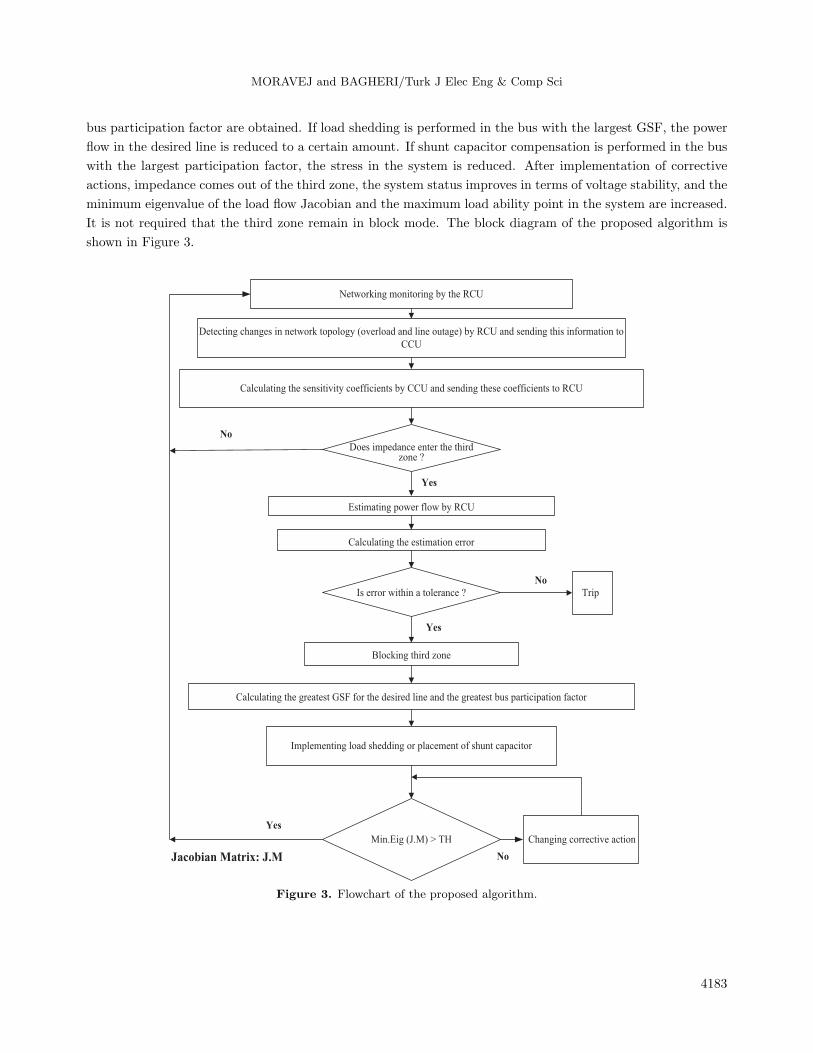
bus participation factor are obtained. If load shedding is performed in the bus with the largest GSF, the power

flow in the desired line is reduced to a certain amount. If shunt capacitor compensation is performed in the bus

with the largest participation factor, the stress in the system is reduced. After implementation of corrective

actions, impedance comes out of the third zone, the system status improves in terms of voltage stability, and the

minimum eigenvalue of the load flow Jacobian and the maximum load ability point in the system are increased.

It is not required that the third zone remain in block mode. The block diagram of the proposed algorithm is

shown in Figure 3.

Networking monitoring by the RCU

Detecting changes in network topology (overload and line outage) by RCU and sending this information to

CCU

Calculating the sensitivity coefficients by CCU and sending these coefficients to RCU

Estimating power flow by RCU

Calculating the estimation error

Calculating the greatest GSF for the desired line and the greatest bus participation factor

Does impedance enter the thirdzone ?

Is error within a tolerance ?

Implementing load shedding or placement of shunt capacitor

Blocking third zone

Min.Eig (J.M) > TH Changing corrective action

Trip

No

No

No

Yes

Yes

Jacobian Matrix: J.M

Yes

Figure 3. Flowchart of the proposed algorithm.

4183


4. Simulation results and analysis

In this section, the proposed algorithm is evaluated for a 14-bus system. A single-line diagram of the 14-bus

test is shown in Figure 4. Data for this test system were obtained from [33]. All load buses are the constant

power type.

C

G

G

C

C

1

2

3

45

6

7

89

10

11

12

13

14

G

C

GENERATORS

SYNCHRONOUS

CONDENSERS

C

THREE

TRANSFORMER

WINDING

EQUIVALENT

4

9

7

8

1 2

543

6

87

12

11 10

91514

13

1716

19 18

22

2121

23

2425

2627

2928

3130

Figure 4. Single-line diagram of the 14-bus test system.

When disturbances are imposed on the system, some margins of the relays in the system become negative,

which causes the relays to trip. If the Z3 relay trips, the system status deteriorates in terms of voltage stability

or the power flow becomes divergent. Voltage stability status is diagnosed with the help of the minimum

eigenvalue of the load flow Jacobian matrix. In the next step, the proposed algorithm acts to improve the

4184


minimum eigenvalue of the load flow Jacobian with the help of load shedding and shunt capacitor compensation.

After the implementation of these corrective actions, the relay margin and minimum eigenvalue of the load flow

Jacobian increases. Load shedding action can reduce stress intensity in the line where the relay is located. After

the implementation of corrective actions, the maximum loadability point increases. Maximum loadability point

is obtained by using the CPF method and modal analysis. At the MLP point, the minimum eigenvalue of all

three Jacobian matrices reaches zero and therefore the Jacobian matrices become singular [15].

During voltage instability, the relay should not send the trip signals where a different corrective action

should be taken, such as load shedding or shunt capacitor compensation [8]. During fault and voltage instability,

apparent impedance seen by the distance relay is low and has possibly entered the third zone.

The third zone settings in this system are calculated according to Section 2.2. These settings have been

set with regard to the effects of infeed.

The sequence of events is described as follows: Initially, the system is in normal condition. First a fault

occurs in line 6-13, and then relays 2 and 23 disconnect this line. Second, the load at bus 13 is increased by

110%. Third, the load at bus 14 is increased by 100%. In these events, second and third disturbances occur

1 s after the previous disturbance. After the occurrence of these disturbances, the margin of relay 26 becomes

equal to –0.0666 and causes the relay to trip. If Z3 of relay 26 trips, the load flow becomes divergent. This

algorithm is able to differentiate between faults and voltage instability.

In the first event, line 6-13 is disconnected. In this case, the LODF is used to estimate the changed

loading after a line tripping. d12−13, d6−13 represents the power flow changing ratio in line 12-13 due to an

outage in line 6-13. The value of this coefficient is 0.6522. After the first event, the relay margin of relay 26

is equal to 2.3983. According to the proposed algorithm, when the relay margin is positive, the RCU will not

attempt to estimate the power flow. However, if the RCU estimates the power flow, the estimated value in

receiving line 12-13 is almost equal to the measured value in receiving line 12-13. The estimation error in this

condition is about 2.2%. This is shown in Table 1.

Table 1. Estimated and measured values in the receiving line 12-13 after each event.

Relay margin Measured value (P.U.) Estimated value (P.U.)2.3983 0.19362 0.19790.4311 0.30718 0.3085–0.066 0.36798 0.3673

The second event occurs after disconnecting line 6-13; the CCU calculates the GSF coefficient with respect

to disconnected line 6-13. a12−13,13 represents the power flow changing ratio in line 12-13 due to a change of

load in bus 13. The value of this coefficient is –0.5528. After this event, the relay margin of relay 26 is equal to

0.4311. If the RCU estimates the power flow, the estimated value in receiving line 12-13 is almost equal to the

measured value in receiving line 12-13. The estimation error in this condition is about 0.4%. This is shown in

Table 1.

After the third event, the relay margin of relay 26 is equal to –0.0666. a12−13,14 represents the power

flow changing ratio in line 12-13 due to change of load in bus 14. The value of this coefficient is –0.2882. In

the proposed algorithm, when the relay margin is negative, the RCU will attempt to estimate the power flow.

From Table 1, it is seen that the estimated value in receiving line 12-13 is almost equal to the measured value

in receiving line 12-13. The estimation error under this condition is about 0.4%. It is seen that the proposed

algorithm prevents the relay operation under this condition.

4185


Under stress conditions in the system, when the power flow estimation is performed at the receiving end

of the line, the error becomes less. By estimating the power flow at the receiving end of the line, more correct

information is obtained from the system status. However, under stress conditions in the system, when the power

flow estimation is performed at the sending end of the line, the error becomes greater.

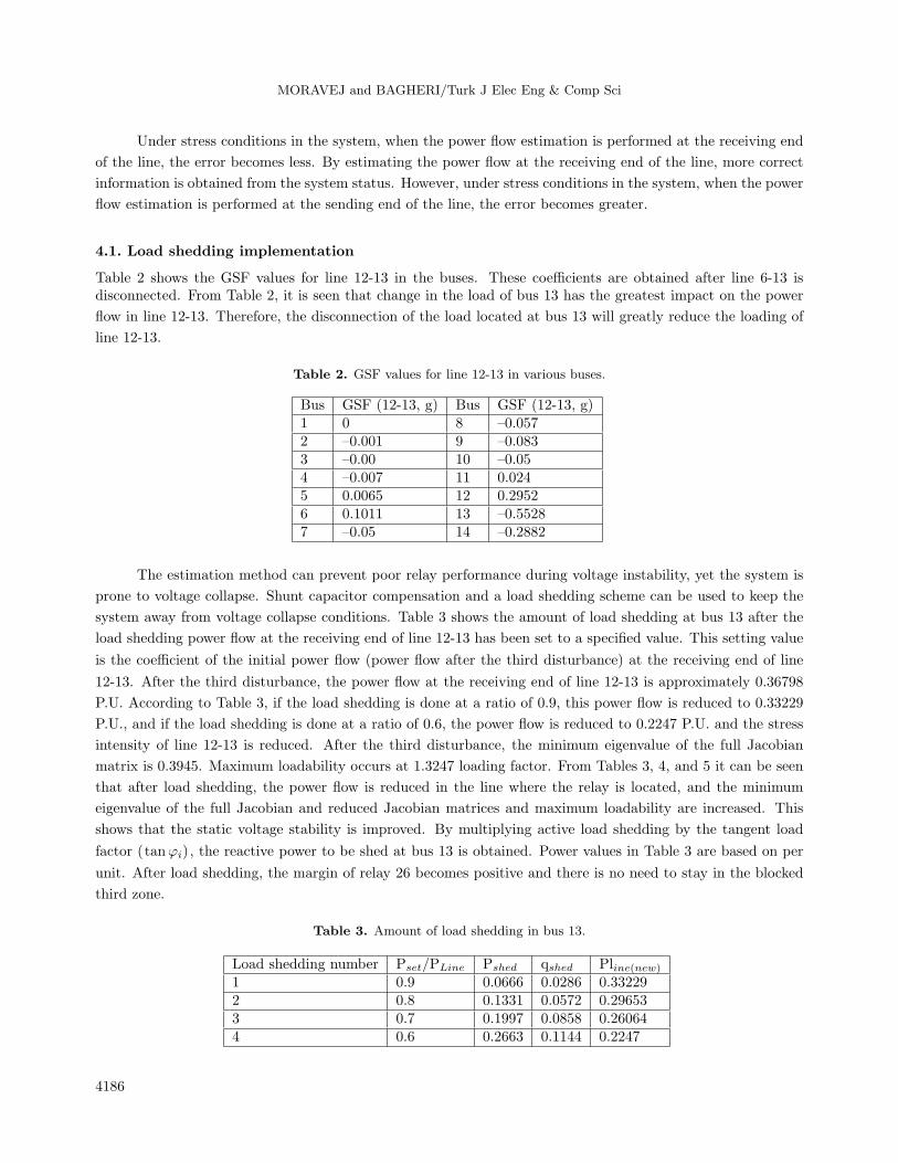
4.1. Load shedding implementation

Table 2 shows the GSF values for line 12-13 in the buses. These coefficients are obtained after line 6-13 isdisconnected. From Table 2, it is seen that change in the load of bus 13 has the greatest impact on the power

flow in line 12-13. Therefore, the disconnection of the load located at bus 13 will greatly reduce the loading of

line 12-13.

Table 2. GSF values for line 12-13 in various buses.

Bus GSF (12-13, g) Bus GSF (12-13, g)1 0 8 –0.0572 –0.001 9 –0.0833 –0.00 10 –0.054 –0.007 11 0.0245 0.0065 12 0.29526 0.1011 13 –0.55287 –0.05 14 –0.2882

The estimation method can prevent poor relay performance during voltage instability, yet the system is

prone to voltage collapse. Shunt capacitor compensation and a load shedding scheme can be used to keep the

system away from voltage collapse conditions. Table 3 shows the amount of load shedding at bus 13 after the

load shedding power flow at the receiving end of line 12-13 has been set to a specified value. This setting value

is the coefficient of the initial power flow (power flow after the third disturbance) at the receiving end of line

12-13. After the third disturbance, the power flow at the receiving end of line 12-13 is approximately 0.36798

P.U. According to Table 3, if the load shedding is done at a ratio of 0.9, this power flow is reduced to 0.33229

P.U., and if the load shedding is done at a ratio of 0.6, the power flow is reduced to 0.2247 P.U. and the stress

intensity of line 12-13 is reduced. After the third disturbance, the minimum eigenvalue of the full Jacobian

matrix is 0.3945. Maximum loadability occurs at 1.3247 loading factor. From Tables 3, 4, and 5 it can be seen

that after load shedding, the power flow is reduced in the line where the relay is located, and the minimum

eigenvalue of the full Jacobian and reduced Jacobian matrices and maximum loadability are increased. This

shows that the static voltage stability is improved. By multiplying active load shedding by the tangent load

factor (tanφi), the reactive power to be shed at bus 13 is obtained. Power values in Table 3 are based on per

unit. After load shedding, the margin of relay 26 becomes positive and there is no need to stay in the blocked

third zone.

Table 3. Amount of load shedding in bus 13.

Load shedding number Pset/PLine Pshed qshed Pline(new)

1 0.9 0.0666 0.0286 0.332292 0.8 0.1331 0.0572 0.296533 0.7 0.1997 0.0858 0.260644 0.6 0.2663 0.1144 0.2247

4186


4.2. Shunt capacitor compensation

After the third disturbance, the minimum eigenvalue of matrix JRQU is equal to 1.1207, the fifth mode of matrix

JRQU . From Table 6, it is seen that the participation factor in bus 13 is higher than in the other load buses.

This shows that shunt capacitor compensation in this bus has the greatest impact on stabilizing the weakest

mode.

P k5= vk5 .w5k , 0 ≤ K ≤ 14 , K = PU bus (18)

The static voltage stability limit can be improved by shunt capacitor compensation in the weakest bus. Shunt

capacitor compensation is performed in bus 13 in order to improve the static voltage stability and relay margin.

From Tables 4 and 5, it is seen that after the occurrence of a disturbance in the system, the minimum eigenvalue

of the full Jacobian matrix, the reduced active and reactive Jacobian matrices, and the maximum loadability are

reduced. At the maximum loadability point, the minimum eigenvalue of the full Jacobian matrix and reduced

Jacobian matrices is zero. For calculating the maximum loadability point, the reactive power limits are not

considered, and this point is analyzed by a combination of the CPF method and modal analysis.

It is seen that after each disturbance in the system, maximum loadability occurs under less loading

factors, which is not appropriate. Therefore, shunt capacitor compensation and a load shedding scheme are

used to increase the maximum loadability and improve the voltage stability of the system.

From Table 4, it is seen that by increasing the susceptance of the capacitor in bus 13, the minimum

eigenvalue of the full Jacobian and reduced Jacobian matrices is increased. Susceptance values in Tables 4, 5,

and 7 are based on per unit. After shunt capacitor compensation in the weak bus, the relay margin is increased

and static voltage stability is improved. Maximum loadability is obtained by using modal analysis and CPF.

Increasing the susceptance of capacitor in the weak bus enhances maximum loadability.

From Figure 5, it is seen that after event 3, impedance loci entered the third zone. By using a power

estimation algorithm, Z3 is blocked under event 3. It is shown that after load shedding and shunt compensation

in bus 13, impedance exits from zone 3 and the relay margin becomes greater.

Table 4. Minimum eigenvalue of the Jacobian matrices after each disturbance and corrective action in the system.

Min (eig (JRPθ)) Min (eig (JRQU)) Min (eig (J))

0.5149 2.5981 0.5147 Normal state

Disturbance

number

0.4726 1.5059 0.4741 1

0.4415 1.3108 0.4384 2

0.4046 1.1207 0.3945 3

0.4212 1.2146 0.4148 1

Load shedding

number

0.4346 1.2915 0.4307 2

0.4459 1.3564 0.4439 3

0.4556 1.412 0.4551 4

0.4108 1.1432 0.4028 0.1

Shunt capacitor

compensation

(susceptance)

0.4169 1.1658 0.4112 0.2

0.4229 1.1889 0.4198 0.3

0.435 1.2372 0.4379 0.5

4187


Table 5. Maximum loadability after each disturbance and corrective action in the system.

Min (eig (JRPθ)) Min (eig (JRQU)) Min (eig (J)) MLP (Loading factor)

5.6919e-4 0.01 5.3871e-4 2.77 Normal state

Disturbance

number

0.0092 0.02 0.0064 2.2697 1

0.007 0.0094 0.004 1.579 2

0.0135 0.0188 0.0079 1.3249 3

0.003 0.0043 0.0018 1.4349 1

Load shedding

number 0.0125 0.0187 0.0076 1.5489 2

0.0129 0.0195 0.0078 1.6628 3

0.0071 0.0105 0.0043 1.7735 4

0.0117 0.0162 0.0069 1.3455 0.1 Shunt capacitor

compensation

(susceptance)

0.0163 0.0223 0.0095 1.3665 0.2

0.0095 0.0126 0.0054 1.3882 0.3

0.0071 0.0091 0.004 1.4331 0.5

Table 6. Participation factor in the load buses.

K 4 5 7 9 10 11 12 13 14P k5 0.0022 0.0012 0.0169 0.0571 0.0487 0.0154 0.1381 0.3956 0.3249

1.5

4

Figure 5. R-X diagram with capacitor compensation and load shedding.

In Figures 6 and 7, the maximum loadability and minimum eigenvalue of the reactive Jacobian matrix

after each disturbance are reduced, and they increase after each load shedding and shunt compensation. Figure

8 shows the continuation curve for each condition in the system. In a normal state, maximum loadability is

equal to 2.77. After the third disturbance, this point is reduced and becomes equal to 1.3249. After 0.5 (P.U.)

shunt compensation in bus 13, maximum loadability is increased to 1.4331. However, if after the third event

0.2663 (P.U.) active load shedding in load bus 13 is performed, the maximum loadability is increased to 1.7735.

Therefore, it is seen that maximum loadability for 0.2663 (P.U.) active load shedding in bus 13 is more than

0.5 (P.U.) shunt compensation in bus 13.

4188


Figure 6. Maximum loadability and minimum eigenvalue of the reactive Jacobian matrix after each event and load

shedding.

Events

Figure 7. Maximum loadability and minimum eigenvalue of the reactive Jacobian matrix after each event and shunt

compensation.

Table 7. Relay margin after each corrective action.

Relay margin

0.21731

Load shedding

number

0.58342

1.063

1.69544

0.18620.1Shunt capacitor

compensation

)susceptance(

0.47630.2

0.78710.3

1.33240.5

4189


Figure 8. Continuation curve for load bus 13 in normal state (solid line), after third disturbance (long-dash line), after

shunt compensation with 0.5 P.U. (dashed dotted line), and after load shedding number 4 (dashed double dotted line).

The use of a shunt capacitor may lead to an unacceptable voltage magnitude in normal operation or with

a low loading factor, and the amount of reactive power delivered is mostly dependent on the voltage magnitude.

Hence, it may increase the power transfer capability, but it will not improve voltage stability compared to the

SVC and STATCOM.

5. Conclusion

In this paper, an improved strategy is presented in order to improve distance protection and system performance

during voltage instability. In addition to preventing undesirable distance relay tripping during voltage instability,

after performing corrective actions, the relay margin became positive and the static voltage stability limit was

increased. In power estimation, if the difference between the measured value and the estimated value is less

than 5% on the receiving end, disturbance condition is identified by the regional control unit and blocks the

third zone of relay under these conditions. The power flow estimation at the receiving end of the line is more

accurate than the power flow estimation at the sending end of the line. After blocking Z3, the system is still

under voltage instability. In order to improve the voltage stability and relay margin, load shedding or shunt

capacitor compensation can be performed. Load shedding and shunt capacitor compensation are performed in

the bus with the largest GSF value and the largest participation factor, respectively. After corrective action,

the static voltage stability and relay margin are improved and the minimum eigenvalues of the full Jacobian

are reduced. While the relay margin becomes positive, the relay does not need to remain blocked. After each

disturbance, maximum loadability decreases. It is found by using modal analysis and continuation power flow

that maximum loadability increases after the corrective action.

References

[1] Kundur P. Power System Stability and Control. 1st ed. New York, NY, USA: McGraw-Hill, 1994.

[2] Kundur P, Paserba J, Ajjarapu V, Anderson G, Bose A, Canizares C. Definition and classification of power system

stability. IEEE T Power Syst 2004; 19: 1387-1401.

4190


[3] Office of Electricity Delivery & Energy Reliability. Final Report on the August 14, 2003 Blackout in the United

States and Canada: Causes and Recommendations. Washington, DC, USA: Office of Electricity Delivery & Energy

Reliability, 2003.

[4] Abidin AF, Mohamed A, Ayob A. A new method to prevent undesirable distance relay tripping during voltage

collapse. Eur J Sci Res 2009; 31: 59-71.

[5] Shen G, Ajjarapu V. A novel algorithm incorporating system status to prevent undesirable protection operation

during voltage instability. In: IEEE 2007 North American Power Symposium; 30 September–2 October 2007; Las

Cruces, NM, USA. New York, NY, USA: IEEE. pp. 373-378.

[6] Smon I, Panto M, Gubina F. An improved voltage collapse protection algorithm based on local phasors. Elec Power

Syst Res 2008; 78: 434-440.

[7] Verbic G, Gubina F. A novel scheme of local protection against voltage collapse based on the apparent power losses.

Int J Elec Power 2004; 26: 341-347.

[8] Abidin FB, Mohamed A. On the use of voltage stability index to prevent undesirable distance relay operation during

voltage instability. In: IEEE 2010 International Conference on Environment and Electrical Engineering; 16–19 May

2010; Czech Republic, Prague. New York, NY, USA: IEEE. pp. 384-387.

[9] Verbic G, Gubina F. A new concept of voltage collapse protection based on local phasors. IEEE T Pow Deliver

2004; 19: 576-581.

[10] Hodaei SAA, Ranjbar AM, Amraee T. Improvement of distance relay performance during voltage instability

conditions. In: IEEE 2009 North American Power Symposium; 4–6 October 2009; Starkville, MS, USA. New

York, NY, USA: IEEE. pp. 1-5.

[11] Jonsson M, Daalder JE. An adaptive scheme to prevent undesirable distance protection operation during voltage

instability. IEEE T Pow Deliver 2003; 18: 1174-1180.

[12] Tang J. Wide area differential protection system. PhD, Florida State University, Tallahassee, FL, USA, 2006.

[13] Gao B, Morison GK, Kundur P. Voltage stability evaluation using modal analysis. IEEE T Power Syst 1992; 7:

1529-1542.

[14] Da Silva LCP, Da Costa VF, Xu W. Preliminary result on improving the modal analysis technique for voltage

stability assessment. In: IEEE 2000 Power Engineering Society Summer Meeting; 16–20 July 2000; Seattle, WA,

USA. New York, NY, USA: IEEE. pp. 1946-1950.

[15] Amjady N, Velayati MH. Evaluation of the maximum loadability point of power systems considering the effect of

static load models. Energ Convers Manage 2009; 50: 3202-3210.

[16] Sauer PW, Lesieutre PC, Pai MA. Maximum loadability and voltage stability in power systems. Int J Elec Power

1993; 15: 145-153.

[17] Tare RS, Bijwe PR. A new index for voltage stability monitoring and enhancement. Int J Elec Power 1998; 20:

345-351.

[18] Arya LD, Sakravdia DK, Kothari DP. Corrective rescheduling for static voltage stability control. Int J Elec Power

2005; 27: 3-12.

[19] Ching YL, Shao HT, Yuan KW. A new approach to the assessment of steady state voltage stability margins using

the P–Q–V curve. Int J Elec Power 2010; 32: 1091-1098.

[20] Arief A, Nappu MB, Yin X, Zhou X, Dong ZY. Under voltage load shedding design with modal analysis approach.

In: IEEE 2009 International Conference on Advances in Power System Control Operation and Management; 8–11

November 2009; Hong Kong. New York, NY, USA: IEEE. pp. 1-5.

[21] Yunus KG, Pinares G, Tuan LA, Tjernberg LB. A combined zone-3 relay blocking and sensitivity based load

shedding for voltage collapse prevention. In: IEEE 2010 Innovative Smart Grid Technologies Conference Europe;

11–13 October 2010; Gothenburg, Sweden. New York, NY, USA: IEEE. pp. 1-8.

4191

http://dx.doi.org/10.1109/NAPS.2007.4402337



http://dx.doi.org/10.1016/j.epsr.2007.03.012


http://dx.doi.org/10.1016/j.ijepes.2003.11.001


http://dx.doi.org/10.1109/TPWRD.2004.824763




http://dx.doi.org/10.1109/59.207377

http://dx.doi.org/10.1109/59.207377

http://dx.doi.org/10.1016/j.enconman.2009.08.026


http://dx.doi.org/10.1016/0142-0615(93)90029-M

http://dx.doi.org/10.1016/0142-0615(93)90029-M

http://dx.doi.org/10.1016/S0142-0615(97)00056-2

http://dx.doi.org/10.1016/S0142-0615(97)00056-2



http://dx.doi.org/10.1049/cp.2009.1822

http://dx.doi.org/10.1049/cp.2009.1822

http://dx.doi.org/10.1049/cp.2009.1822

http://dx.doi.org/10.1109/ISGTEUROPE.2010.5638944




[22] Lopes BIL, De Souza ACZ. An approach for under voltage load shedding. In: IEEE 2003 Power Tech Conference;

23–26 June 2003; Bologna, Italy. New York, NY, USA: IEEE. pp. 1-5.

[23] Arya LD, Choube SC, Shrivastava M. Technique for voltage stability assessment using newly developed line voltage

stability index. Energ Convers Manage 2008; 49: 267-275.

[24] Boonpirom N, Paitoonwattanakij K. Static voltage stability enhancement using Facts. In: IEEE 2005 International

Power Engineering Conference; 29 November–2 December 2005; Singapore. New York, NY, USA: IEEE. pp. 711-715.

[25] Perez MA, Messina AR, Esquivel CRF. Application of FACTS devices to improve steady state voltage stability.

In: IEEE 2000 Power Engineering Society Summer Meeting; 16–20 July 2000; Seattle, WA, USA. New York, NY,

USA: IEEE. pp. 1115-1120.

[26] Dobraca F, Pai MA, Sauer PW. Relay margin as a tool for dynamical security analysis. Int J Elec Power 1990; 12:

226-234.

[27] Bai H, Ajjarapu V. Transmission system vulnerability assessment based on practical identification of critical relays

and contingencies. In: IEEE 2008 Power and Energy Society General Meeting; 20–24 July 2008; Pittsburgh, PA,

USA. New York, NY, USA: IEEE. pp. 1-8.

[28] Leung KW. Computer aided setting calculation for distance zone 2 and zone 3 protection. In: IET 1991 International

Conference on Advances in Power System Control Operation and Management; 5–8 November 1991; Hong Kong.

Stevenage, UK: IET. pp. 152-157.

[29] Horowitz SH, Phadke AG. Third zone revisited. IEEE T Pow Deliver 2006; 21: 23-29.

[30] Moravej Z, Jazaeri M, Gholamzadeh M. Optimal coordination of distance and over current relays in series compen-

sated system based on MAPSO. Energ Convers Manage 2012; 56: 140-151.

[31] Seong L. Zone 3 relay blocking scheme to prevent cascaded events. T Tianjin Univ 2008; 14: 97-105.

[32] Nagendra P, Dey SH, Paul S, Datta T. A novel approach for global voltage stability assessment of a power system

incorporating static var compensator. Eur T Elec Power 2012; 22: 1016-1026.

[33] Lee SH, Liu JH, Chu CC. Modelling and locating unified power flow controllers for static voltage stability enhance-

ments. Int T Elec Energ Syst 2012; 24: 1-17.

[34] Mansour MR, Geraldi EL, Costa ALF, Ramos RA. A new and fast method for preventive control selection in voltage

stability analysis. IEEE T Power Syst 2013; 28: 4448-4455.

[35] Aman MM, Jasmon GB, Bakar AHA, Mokhlis H. Optimum network reconfiguration based on maximization of

system loadability using continuation power flow theorem. Elec Power Energ Syst 2014; 54: 123-133.

[36] Tobon JE, Ramirez JM, Gutierrez REC. Tracking the maximum power transfer and loadability limit from sensitiv-

ities based impedance matching. Elec Power Syst Res 2015; 119: 355-363.

[37] Salgado R, Takashiba J. A framework to study QV constraint exchange points in the maximum loadability analysis.

Elec Power Energ Syst 2015; 64: 347-355.

4192

http://dx.doi.org/10.1109/PTC.2003.1304174

http://dx.doi.org/10.1109/PTC.2003.1304174



http://dx.doi.org/10.1109/IPEC.2005.207000

http://dx.doi.org/10.1109/IPEC.2005.207000

http://dx.doi.org/10.1109/PESS.2000.867535



http://dx.doi.org/10.1016/0142-0615(90)90038-D

http://dx.doi.org/10.1016/0142-0615(90)90038-D




http://dx.doi.org/10.1002/etep.623

http://dx.doi.org/10.1002/etep.623

http://dx.doi.org/10.1109/TPWRS.2013.2268013

http://dx.doi.org/10.1109/TPWRS.2013.2268013







Documents

Assessment of the maximum loadability point of a power